ISSN 1344-8803, CSSE-20 June 18, 2004

State-Dependent Scaling Characterization forInterconnected Nonlinear Systems–Part I:

Constructive Generalization of Stability Criteria¶§

Hiroshi Ito†‡

† Dept. of Systems Innovation and InformaticsKyushu Institute of Technology

680-4 Kawazu, Iizuka, Fukuoka 820-8502, JapanPhone: +81 948-29-7717, Fax: +81 948-29-7709

E-mail: hiroshi@ces.kyutech.ac.jp

Abstract: This paper is concerned with the problem of global stability and performanceof nonlinear interconnected systems. The state-dependent scaling problem is proposedas a unified mathematical formulation whose solutions explicitly provide Lyapunov func-tions proving stability and dissipative properties of feedback and cascade systems. Theframework covers nonlinear systems having diverse and strong nonlinearities representedby general supply rates. Previously existing stability theorems such as the L2 small-gaintheorem, the passivity theorems, the circle and Popov criteria and the input-to-statestable(ISS) small-gain theorem are extracted from the framework as special elementarycases. Indeed, those existing stability criteria are sufficient conditions for the existenceof solutions to the state-dependent scaling problems, and the solutions can be shownexplicitly. A notable benefit of the proposed formulation is that it actually yields usefulanswers for systems disagreeing with classical and ISS nonlinearities, which is much morethan formal applicability. The paper focuses on generalization and unification, while thefollow-up paper puts a special emphasis on theoretical demonstration of the effectivenessof the state-dependent scaling characterization.

Keywords: Nonlinear interconnected system, Global asymptotic stability, Lyapunov func-tion, Stability criteria, Dissipative system, Supply rates, State-dependent scaling,

¶Technical Report in Computer Science and Systems Engineering, Log Number CSSE-20, ISSN 1344-8803. c©2004Kyushu Institute of Technology

§Early versions of this paper were presented in the 41st IEEE Conf. Decision Control, pp.3937-3943, Las Vegas,USA, December 13, 2002, and SICE 2nd Annual Conference on Control Systems, pp.81-86, Chiba, Japan, May 30,2002.

‡Author for correspondence

1

1 Introduction

In the literature of nonlinear control theory, a great deal of effort has been put into the problemof finding useful formulations of conditions under which interconnected systems are stable. Oneof significant contributions is the stability theory developed in [1], which unifies previously knownstability criteria and provides Lyapunov versions of input-output stability results such as the L2 small-gain theorem, the passivity theorems, and the circle and Popov criteria. Another major developmentwhich presently plays an important role in nonlinear control analysis and design is the ISS small-gaintheorem also known as the nonlinear small-gain theorem[2, 3]. A small-gain theorem which broughtabout the ISS small-gain theorem was originally formulated by Hill[4], and Mareels and Hill[5], andthat was extended in the ISS framework by Jiang et al.[2] which was also further generalized byTeel[3]. The effectiveness of the ISS small-gain theorem is evident when systems have essentialnonlinearities described by the input-to-state stable(ISS) property[6]. It is, however, known thatthere are systems for which ISS is too strong requirement. One has yet to develop a stability theorywhich encompasses much broader classes of systems in dealing with interconnections of nonlinearsystems.

The main purpose of the paper is to propose a general approach to the stability and performanceof nonlinear interconnected systems. We need a framework which is not limited to the settingsof popular classical stability criteria and the ISS small-gain theorem. The goal of this paper isthe development of a general framework from which the set of presently known important resultscan be easily extracted as special cases. To this end, this paper borrows an idea from the state-dependent scaling techniques which have been recently introduced by the author[7, 8, 9], and thispaper generalizes it much further. The main product of this paper is the formulation of the state-dependent scaling problems. The state-dependent scaling problems are scalar inequalities we solvefor parameters. The parameters are called state-dependent scaling functions in this paper. Thepoints this paper addresses include three main issues. One is to show that problems of stability andperformance analysis for interconnected dissipative systems can be reduced into the state-dependentscaling problems in a unified way. Another is to clarify when solutions of the state-dependent scalingproblems exist. The other is to demonstrate how we are able to calculate the solutions explicitly.

The techniques employed by [7, 8, 9] can be considered as primitive versions and limited specialcases of the general results developed in this paper. The usefulness of the idea of state-dependentscaling in constructing robust control Lyapunov functions has been demonstrated in [8, 9] for severaldesign problems of robust nonlinear controllers. However, discussion about connections with otherapproaches has not been given in the literature. One of objectives of this paper is to clarify forthe first time the relation between the state-dependent scaling formulation and the ISS small-gaincondition[2, 3] as well as stability criteria for dissipative systems[1].

One of benefits from the developments in this paper is that the ISS small-gain theorem and thedissipative approach can be explained in a unified language. The ISS small-gain theorem and its proofare usually given in terms of trajectories of systems(or input-output-type formulation)[2, 3, 10]. Anotable exception is [11] which presents non-smooth functions guaranteeing the existence of Lyapunovfunctions. However, the result has not yielded an explicit formula to directly obtain smooth Lyapunovfunctions which are useful for controller design. The ISS small-gain condition by itself does not showexplicit information about how to construct Lyapunov functions. We sometimes prefer constructivetools since we rely on Lyapunov functions in many cases of nonlinear systems design when systemmodels are given. The storage function which plays a key role in the dissipative analysis[12, 1] servesas a Lyapunov function. The storage function is an abstract notion of energy stored in a system.The energy increases when energy is supplied from outside. The supply rate determines the variation

2

of the storage function. The idea proposed in [1] is to define the storage function of interconnectedsystems by summing up supply rates of individual systems. Although the ISS property of open-loopsystems has been related to the existence of Lyapunov functions[13, 14, 10], little development hasbeen made in the construction of Lyapunov functions for feedback systems. This background hascreated a gap between the dissipative approach and the ISS small-gain theorem. This paper offersa new avenue to the ISS small-gain theorem, and it closes the gap successfully. This paper comesat an idea of summing up supply rates nonlinearly for constructing a Lyapunov function for theISS small-gain theorem. Calculation of nonlinear coefficients to combine supply rates for the ISSsmall-gain theorem and calculation of constant coefficients for the dissipative approach are unifiedinto solutions to the state-dependent problems.

Another major advantage of the state-dependent scaling approach over the existing stability criteriais that it is applicable to systems whose nonlinearity disagrees with ISS and other classical nonlin-earities. It is not only applicable, but also surely effective so that useful answers can be obtained forbroader classes of essentially nonlinear systems. This paper demonstrates it through some examples.Theoretical demonstration of the effectiveness is a very important issue on which the authors put aspecial emphasis. The follow-up paper is devoted to the discussion and gives interesting evidences ofthe universality beyond formal applicability.

This paper is organized as follows. In Section 2, we presents a mathematical problem of state-dependent scaling which forms the main idea of this paper. Several variants of the state-dependentscaling problem are formulated by introducing little modification into the main problem. Theseproblems are closely connected each other by a simple inclusive relation. In Section 3, we define anonlinear interconnected system. A general configuration is employed to deal with feedback systemsand cascade systems in a unified manner. Then, solutions to the state-dependent scaling problemsare related explicitly to the construction of Lyapunov functions of the interconnected system. Thecentral inequality of the state-dependent scaling problems is given an interpretation of the sum ofnonlinearly scaled supply rates of dissipative systems. It is shown that properties of stability anddisturbance attenuation can be established for the interconnected system once we have obtaineda solution to the state-dependent scaling problems. Thereby, we propose a unified approach toanalysis of stability and performance of interconnected dissipative systems. In Section 4, the ideaand the effectiveness of the approach are illustrated through several examples involving nonlinearitieswhich are not covered by the classical stability criteria and the ISS small-gain theorem. Section 5 isconcentrated on supply rates which are popular in classical stability analysis such as the L2 small-gain theorem, the passivity theorems, and the circle and Popov criteria. It is explained that thoseclassical stability criteria are based on linear combination of supply rates, which are proved to be theeasiest cases of the state-dependent scaling problems. Section 6 deals with supply rates of the ISSproperty. The ISS small-gain theorem is explained in the state-dependent scaling framework, and theinterconnection of ISS systems is considered as an example for which nonlinear combination of supplyrates is essential. Using Section 5 and Section 6, the author demonstrates that the classical stabilitytheorems and the ISS small-gain theorem can be extracted as special cases of the state-dependentscaling formulation. Stability conditions provided by classical stability criteria and the ISS small-gaintheorem are viewed as sufficient conditions for guaranteeing the existence of solutions to the state-dependent scaling problems. Finally, conclusions are drawn in Section 7. The follow-up paper [15]gives a deep insight into the effectiveness of the state-dependent scaling approach by theoreticallyaddressing the question of how solutions to the state-dependent scaling problems are obtained foradvanced types of nonlinearities which are not covered by popular classical and advanced stabilitycriteria available previously.

This paper uses the following notations. The interval [0,∞) in the space of real numbers R is

3

Σ1 : x1 =f1(t, x1,u1, r1)

Σ2 : x2 =f2(t, x2,u2, r2)

¾

-

¾

-x2

x1r1

r2

u1

u2

Figure 1: Feedback interconnected system Σ

denoted by R+. Euclidean norm of a vector in Rn of dimension n is denoted by | · |. A functionγ : R+ → R+ is said to be class K and written as γ ∈ K if it is a continuous, strictly increasingfunction satisfying γ(0) = 0. A function γ : R+ → R+ is said to be class K∞ and written as γ ∈ K∞if it is a class K function satisfying limr→∞ γ(r) = ∞.

2 State-dependent scaling problems

This section presents a main mathematical problem which plays a central role in this paper, andintroduces several variants of the main problem. We refer to the mathematical problems as the state-dependent scaling problems. Interpretation and importance of the problems in nonlinear systemscontrol will be discussed in subsequent sections.

The following defines our main mathematical problem which contains the primary idea of thestate-dependent scaling framework.

Problem 1 Given continuously differentiable functions Vi : (t, xi) ∈ R+×Rni → R+ and continuousfunctions ρi : (xi, xj , ri) ∈ Rni × Rnj × Rmi → R for i = 1, 2 and j = {1, 2} \ {i}, find continuousfunctions λi : s ∈ R+ → R+ satisfying

λi(s) > 0 ∀s ∈ (0,∞) (1)

lims→0+

λi(s) < ∞ (2)∫ ∞

1λi(s)ds = ∞ (3)

for i = 1, 2 such that

λ1(V1(t, x1))ρ1(x1, x2, r1) + λ2(V2(t, x2))ρ2(x2, x1, r2) ≤ ρe(x1, x2, r1, r2),∀x1∈Rn1 , x2∈Rn2 , r1∈Rm1 , r2∈Rm2 , t∈R+ (4)

holds for some continuous function ρe : (x1, x2, r1, r2) ∈ Rn1 × Rn2 × Rm1 × Rm2 → R satisfying

ρe(x1, x2, 0, 0) < 0 , ∀(x1, x2) ∈ Rn1 × Rn2 \ {(0, 0)} (5)

The following is a variant of Problem 1.

Problem 2 Given a continuously differentiable function V2 : (t, x2) ∈ R+×Rn2 → R+ and continu-ous functions ρ1 : (z1, x2, r1) ∈ Rp1×Rn2×Rm1 → R and ρ2 : (x2, z1, r2) ∈ Rn2×Rp1×Rm2 → R, findcontinuous functions λ1 : (t, z1, x2, r1, r2) ∈ R+ ×Rp1 ×Rn2 ×Rm1 ×Rm2 → R+, λ2 : s ∈ R+ → R+,an increasing continuous function ξ1 : s ∈ [0, N ] → R+ and a continuous function ϕ1 : (z1, x2, r1) ∈Rp1 × Rn2 × Rm1 → R+ satisfying

λ2(s) > 0 ∀s ∈ (0,∞) (6)

4

lims→0+

λ2(s) < ∞ (7)∫ ∞

1λ2(s)ds = ∞ (8)

ξ1(s) ≥ 0 ∀s ∈ [0, N ] (9)

ϕ1(z1, x2, r1) ≥ 0, ∀z1∈Rp1 , x2∈Rn2 , r1∈Rm1 (10)

such that

λ1(t, z1, x2, r1, r2) [−ξ1(ϕ1(z1, x2, r1)) + ξ1(ϕ1(z1, x2, r1) + ρ1(z1, x2, r1))] +

λ2(V2(t, x2))ρ2(x2, z1, r2) ≤ ρe(x2, r1, r2),

∀z1∈Rp1 , x2∈Rn2 , r1∈Rm1 , r2∈Rm2 , t∈R+ (11)

holds for some continuous function ρe : (x2, r1, r2) ∈ Rn2 × Rm1 × Rm2 → R satisfying

ρe(x2, 0, 0) < 0 , ∀x ∈ Rn2 \ {0} (12)

where N ∈ [0,∞] is defined by

N = sup(z1,x2,r1)∈Rp1×Rn2×Rm1

[ϕ1(z1, x2, r1) + ρ1(z1, x2, r1))] (13)

In this paper, the functions λi and ξi are referred to as state-dependent scaling functions. Theinequalities (4) and (11) are key formulas on which interpretations will be put later on. The reasonof using the terminology “state-dependent scaling” will be also clear in the next section. Note that(2) and (7) are redundant mathematically since each λi is supposed to be continuous on R+ = [0,∞).The explicit statement of (2) and (7) may be helpful to direct the readers’ attention to it.

This paper calls a pair of λ1 and λ2 a solution to Problem 1 if the pair fulfills all requirementsstated in Problem 1. In a similar manner, a quartet of λ1, λ2, ξ1 and ϕ1 fulfilling all requirementsstated in Problem 2 is called a solution to Problem 2. If we take ξ1(s) = s, the inequality (11)becomes

λ1(t, z1, x2, r1, r2)ρ1(z1, x2, r1) + λ2(V2(t, x2))ρ2(x2, z1, r2) ≤ ρe(x2, r1, r2),

∀z1∈Rp1 , x2∈Rn2 , r1∈Rm1 , r2∈Rm2 , t∈R+ (14)

In the same way, whenever the function ξ1(s) is affine in s, the function ϕ1 disappears from (11).Therefore, in the case of affine ξ1(s), a triplet of λ1, λ2 and ξ1 is called a solution to Problem 2.

At first glance, Problem 2 is complicated since it has more parameters than Problem 1. It is,however, milder than Problem 1. In other words, Problem 1 has a solution only if so does Problem2. It is verified by considering a choice ξ1(s) = s in Problem 2 with p1 = n1. Indeed, the claim canbe obtain easily from (14) and the following lemma.

Lemma 1 Suppose that a continuous function ρe : (x1, x2, r1, r2) ∈ Rn1 × Rn2 × Rm1 × Rm2 → Rsatisfies

ρe(x1, x2, 0, 0) < 0 , ∀(x1, x2) ∈ Rn1 × Rn2 \ {(0, 0)} (15)

(i) If the function ρe satisfies

supx1∈Rn1

ρe(x1, x2, r1, r2) < +∞, ∀(x2, r1, r2) ∈ Rn2 × Rm1 × Rm2 (16)

supx1∈Rn1

ρe(x1, x2, 0, 0) < 0, ∀x2 ∈ Rn2 \ {0} (17)

5

then there exists a continuous function ρe : (x2, r1, r2) ∈ Rn2 × Rm1 × Rm2 → R such that

ρe(x2, 0, 0) < 0 , ∀x2 ∈ Rn2 \ {0} (18)

ρe(x1, x2, r1, r2) ≤ ρe(x2, r1, r2), ∀(x1, x2, r1, r2) ∈ Rn1 × Rn2 × Rm1 × Rm2 (19)

hold.

(ii) If the vector x1 is a dependent variable, and there exists a continuous function g12 : (x2, r1, r2) ∈Rn2 × Rm1 × Rm2 → R+ such that

|x1| ≤ g12(x2, r1, r2) (20)

is satisfied, then there exists a continuous function ρe : (x2, r1, r2) ∈ Rn2 × Rm1 × Rm2 → Rsuch that (18) and

ρe(x1, x2, r1, r2) ≤ ρe(x2, r1, r2), ∀(x2, r1, r2) ∈ Rn2 × Rm1 × Rm2 (21)

hold.

Materials focused on by subsequent sections are the situations of (i) and (ii) in the above lemma.

In this paper, we also consider several other variants which relax Problem 1 and Problem 2. Wedefine Problem 1’ by replacing the condition (5) with

ρe(x1, x2, 0, 0) ≤ 0 , ∀(x1, x2) ∈ Rn1 × Rn2 (22)

Clearly, Problem 1 is solvable only if Problem 1’ has a solution. In the same manner, we defineProblem 2’ by replacing the condition (12) with

ρe(x2, 0, 0) ≤ 0 , ∀x2 ∈ Rn2 (23)

Problem 2 is solvable only if Problem 2’ has a solution. Again, it is easily seen from (14) that Problem1’ is solvable only if Problem 2’ has a solution.

3 Construction of Lyapunov functions

This section demonstrates that stable properties of nonlinear interconnected systems are stronglyrelated to the solutions of the state-dependent scaling problems introduced in Section 2. It is shownthat the inequalities of the sum of scaled supply rates, which are (4) an (11), directly lead us toLyapunov functions establishing the stability of interconnection of dissipative systems in a unifiedmanner.

Consider the nonlinear interconnected system Σ shown in Fig.1. Suppose that subsystems Σ1 andΣ2 are described by

Σ1 : x1 = f1(t, x1, u1, r1) (24)

Σ2 : x2 = f2(t, x2, u2, r2) (25)

These two dynamic systems are connected each other through u1 = x2 and u2 = x1. If Σ1 is static,we suppose that Σ1 is described by

Σ1 : z1 = h1(t, u1, r1) (26)

6

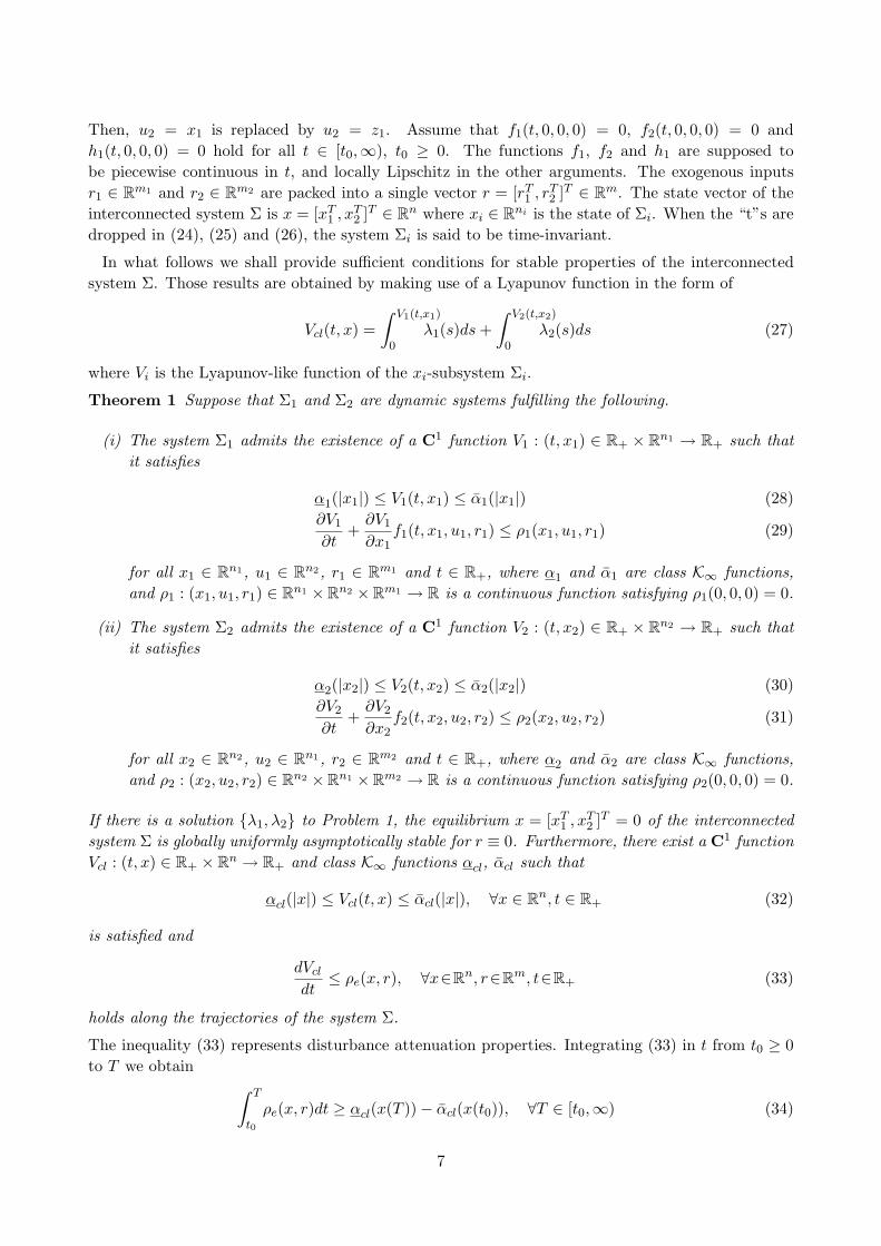
Then, u2 = x1 is replaced by u2 = z1. Assume that f1(t, 0, 0, 0) = 0, f2(t, 0, 0, 0) = 0 andh1(t, 0, 0, 0) = 0 hold for all t ∈ [t0,∞), t0 ≥ 0. The functions f1, f2 and h1 are supposed tobe piecewise continuous in t, and locally Lipschitz in the other arguments. The exogenous inputsr1 ∈ Rm1 and r2 ∈ Rm2 are packed into a single vector r = [rT

1 , rT2 ]T ∈ Rm. The state vector of the

interconnected system Σ is x = [xT1 , xT

2 ]T ∈ Rn where xi ∈ Rni is the state of Σi. When the “t”s aredropped in (24), (25) and (26), the system Σi is said to be time-invariant.

In what follows we shall provide sufficient conditions for stable properties of the interconnectedsystem Σ. Those results are obtained by making use of a Lyapunov function in the form of

Vcl(t, x) =∫ V1(t,x1)

0λ1(s)ds +

∫ V2(t,x2)

0λ2(s)ds (27)

where Vi is the Lyapunov-like function of the xi-subsystem Σi.

Theorem 1 Suppose that Σ1 and Σ2 are dynamic systems fulfilling the following.

(i) The system Σ1 admits the existence of a C1 function V1 : (t, x1) ∈ R+ × Rn1 → R+ such thatit satisfies

α1(|x1|) ≤ V1(t, x1) ≤ α1(|x1|) (28)∂V1

∂t+

∂V1

∂x1f1(t, x1, u1, r1) ≤ ρ1(x1, u1, r1) (29)

for all x1 ∈ Rn1, u1 ∈ Rn2, r1 ∈ Rm1 and t ∈ R+, where α1 and α1 are class K∞ functions,and ρ1 : (x1, u1, r1) ∈ Rn1 ×Rn2 ×Rm1 → R is a continuous function satisfying ρ1(0, 0, 0) = 0.

(ii) The system Σ2 admits the existence of a C1 function V2 : (t, x2) ∈ R+ × Rn2 → R+ such thatit satisfies

α2(|x2|) ≤ V2(t, x2) ≤ α2(|x2|) (30)∂V2

∂t+

∂V2

∂x2f2(t, x2, u2, r2) ≤ ρ2(x2, u2, r2) (31)

for all x2 ∈ Rn2, u2 ∈ Rn1, r2 ∈ Rm2 and t ∈ R+, where α2 and α2 are class K∞ functions,and ρ2 : (x2, u2, r2) ∈ Rn2 ×Rn1 ×Rm2 → R is a continuous function satisfying ρ2(0, 0, 0) = 0.

If there is a solution {λ1, λ2} to Problem 1, the equilibrium x = [xT1 , xT

2 ]T = 0 of the interconnectedsystem Σ is globally uniformly asymptotically stable for r ≡ 0. Furthermore, there exist a C1 functionVcl : (t, x) ∈ R+ × Rn → R+ and class K∞ functions αcl, αcl such that

αcl(|x|) ≤ Vcl(t, x) ≤ αcl(|x|), ∀x ∈ Rn, t ∈ R+ (32)

is satisfied and

dVcl

dt≤ ρe(x, r), ∀x∈Rn, r∈Rm, t∈R+ (33)

holds along the trajectories of the system Σ.

The inequality (33) represents disturbance attenuation properties. Integrating (33) in t from t0 ≥ 0to T we obtain

∫ T

t0

ρe(x, r)dt ≥ αcl(x(T ))− αcl(x(t0)), ∀T ∈ [t0,∞) (34)

7

For instance, by choosing ρe(x, r) as

ρe(x, r) = −|x|p + γp|r|p, p > 0

the inequality (34) with x(t0) = 0 becomes∫ T

t0

γp|r|pdt ≥∫ T

t0

|x|pdt, ∀T ∈ [t0,∞)

which represents Lp disturbance attenuation of level γ. The L2 disturbance attenuation is a popularperformance index for linear systems and it is called H∞ norm of stable linear systems.

The condition (3) requires certain growth order of the function λi(s) with respect to s toward ∞.For instance, s2, s, 1 and 1/(s + 1) are admitted. However, 1/(s2 + 1) and 1/(s3 + 1) do not meetthe condition (3). If λi(s) is continuous and satisfies

λi(s) ≥ k∞s−1, ∀s ∈ [1,∞)

for some k∞ > 0, it fulfills (3). This growth order assumption ensures that the Lyapunov functionVcl(t, x) constructed by (27) is radially unbounded, which leads us to the global stability of Σ.

If a system Σi in Fig.1 is static, the growth order constraint (3) on λi(s) is unnecessary. In addition,we can employ other flexibilities of functions ξi and ϕi. Thereby, Problem 1 can be replaced by aweaker Problem 2 in the presence of a static system.

Theorem 2 Suppose that Σ1 is a static system, and Σ2 is a dynamic system fulfilling the following.

(i) The system Σ1 satisfies

ρ1(z1, u1, r1) ≥ 0 (35)

for all u1 ∈ Rn2 , r1 ∈ Rm1 and t ∈ R+, where ρ1 : (z1, u1, r1) ∈ Rp1 × Rn1 × Rm1 → R is acontinuous function satisfying ρ1(0, 0, 0)=0.

(ii) The system Σ2 satisfies (ii) of Theorem 1.

If there is a solution {λ1, λ2, ξ1, ϕ1} to Problem 2, the equilibrium x = x2 = 0 of the interconnectedsystem Σ is globally uniformly asymptotically stable for r ≡ 0. Furthermore, there exist a C1 functionVcl : (t, x2) ∈ R+ × Rn2 → R+ and class K∞ functions αcl, αcl such that

αcl(|x2|) ≤ Vcl(t, x2) ≤ αcl(|x2|), ∀x2 ∈ Rn2 , t ∈ R+ (36)

is satisfied and

dVcl

dt≤ ρe(x2, r), ∀x2∈Rn2 , r∈Rm, t∈R+ (37)

holds along the trajectories of the system Σ.

A Lyapunov function proving the above theorem is

Vcl(t, x2) =∫ V2(t,x2)

0λ2(s)ds (38)

Using another type of Lyapunov function which is different from the previous theorems, we can alsoestablish the stability in the following way.

8

Theorem 3 Suppose that Σ1 is a static system, and Σ2 is a dynamic system fulfilling the following.

(i) The system Σ1 satisfies (i) of Theorem 2.

(ii) The system Σ2 admits the existence of a C1 function V2 : (t, x2) ∈ R+ × Rn2 → R+ such thatit satisfies

α2(|x2|) ≤ V2(t, x2) ≤ α2(|x2|) (39)∂V2

∂t+

∂V2

∂x2f2(t, x2, u2, r2) ≤ ρ2(x2, u2, r2)− ω2(µ2(x2))

dµ2(x2)dt

(40)

for all x2 ∈ Rn2, u2 ∈ Rn1, r2 ∈ Rm2 and t ∈ R+, where α2 and α2 are class K∞ functions, andρ2 : (x2, u2, r2) ∈ Rn2 ×Rn1 ×Rm2 → R is a continuous function satisfying ρ2(0, 0, 0) = 0, andµ2 : x2 ∈ Rn2 → R is a C1 function satisfying µ2(0) = 0, and ω2 : s ∈ R → R is a continuousfunction satisfying sω2(s) ≥ 0 for all s ∈ R.

If there is a solution {λ1, λ2, ξ1, ϕ1} to Problem 2 and λ2 is constant, then the equilibrium x = x2 = 0of the interconnected system Σ is globally uniformly asymptotically stable for r ≡ 0. Furthermore,there exist a C1 function Vcl : (t, x2) ∈ R+ × Rn2 → R+ and class K∞ functions αcl, αcl such that

αcl(|x2|) ≤ Vcl(t, x2) ≤ αcl(|x2|), ∀x2 ∈ Rn2 , t ∈ R+ (41)

is satisfied and

dVcl

dt≤ ρe(x2, r), ∀x2∈Rn2 , r∈Rm, t∈R+ (42)

holds along the trajectories of the system Σ.

This theorem is based on the following Lyapunov function.

Vcl(t, x2) = λ2V2(t, x2) + λ2

∫ µ2(x2)

0ω2(s)ds (43)

A system Σ1 satisfying (29) is said to be dissipative[12, 1, 16], and the function ρ1 is referred toas the supply rate. In the rest of this paper, a system Σi is said to accept a supply rate ρi if thereexists a C1 function Vi(t, xi) and class K∞ functions αi, αi such that

αi(|xi|) ≤ Vi(t, xi) ≤ αi(|xi|) (44)∂Vi

∂t+

∂Vi

∂xifi(t, xi, ui, ri) ≤ ρi(xi, ui, ri) (45)

hold for all xi, ui, ri and t. When Σi is static, we replace the pair of (44) and (45) by the followingsingle inequality.

ρi(zi, ui, ri) ≥ 0 (46)

For convenience, we call the function ρi for the static system the supply rate although energy is neverstored by static systems.

The conditions (4) and (11) are given in terms of the relation between supply rates of two subsys-tems. It is stressed that the conditions are not in the form of linear combinations of supply rates.Functional coefficients λ1, λ2 and ξ1 are introduced into the combinations of supply rates, and theyscale supply rates of subsystems. The functionals also appear in (27), (38) and (43) to construct

9

the Lyapunov functions. The use of the functionals λ1 λ2 and ξ1 is contrasted with the early workson Lyapunov stability criteria for interconnected dissipative systems such as [12, 1, 16], where linearcombinations of supply rates were employed without such functional coefficients. In (4) and (11), theparameters λ1, λ2 and ξ1 are allowed to be functions of the state variables x1 and x2. This is whythis paper refers to λ1, λ2 and ξ1 as state-dependent scaling functions. State-dependence of scalingfactors is emphasized to distinguish them from constant λ1 and λ2 and an identity function ξ1(s) = s.The conditions (4) and (11) can be regarded as a general formulation of the state-dependent scalingtechnique [7, 8, 9]. The results in [7, 8, 9] were developed on the basis of special cases of (4) and(11) where the supply rates are finite L2-gain, ISS or a subset of integral ISS. Those papers [7, 8, 9]originally refer to 1/λi as the state-dependent scaling factors.

If both the systems Σ1 and Σ2 are time-invariant, stability of interconnected systems can beestablished by solving Problem 1’ and Problem 2’ which are milder than Problem 1 and Problem 2,respectively.

Corollary 1 Suppose that Σ1 and Σ2 are time-invariant dynamic systems satisfying (i) and (ii) ofTheorem 1 with V1(x1) and V2(x2), respectively. If there is a solution {λ1, λ2} to Problem 1’ and

r(t) = 0x(t) ∈ Z

}∀t ∈ R+ ⇒ lim

t→∞x(t) = 0 (47)

holds for the set Z ∈ {x ∈ Rn : ρe(x, 0) = 0}, then the equilibrium x = [xT1 , xT

2 ]T = 0 of the time-invariant interconnected system Σ is globally asymptotically stable for r ≡ 0. Furthermore, thereexist a C1 function Vcl : x ∈ Rn → R+ and class K∞ functions αcl, αcl such that (32) is satisfiedand (33) holds along the trajectories of the system Σ.

Corollary 2 Suppose that Σ1 is a time-invariant static system satisfying (i) of Theorem 2, and Σ2

is a time-invariant dynamic system satisfying (ii) of Theorem 2 with V2(x2) . If there is a solution{λ1, λ2, ξ1, ϕ1} to Problem 2’ and either of

(I) For the set Z2 = {x2 ∈ Rn2 : ρe(x2, 0) = 0},

r(t) = 0x2(t) ∈ Z2

}∀t ∈ R+ ⇒ lim

t→∞x2(t) = 0 (48)

(II) For the set Z2 = {x2 ∈ Rn2 : ρ1(h1(x2, 0), x2, 0) = 0},

u2(t) = h1(x2, 0)r2(t) = 0x2(t) ∈ Z2

∀t ∈ R+ ⇒ lim

t→∞x2(t) = 0 (49)

hold, and there exists a constant ε such that

λ1(t, z1, x2, r1, r2) ≥ ε > 0, ∀z1∈Rp1 , x2∈Rn2 , r1∈Rm1 , r2∈Rm2 , t∈R+ (50)

is fulfilled, then the equilibrium x = x2 = 0 of the time-invariant interconnected system Σ is globallyasymptotically stable for r ≡ 0. Furthermore, there exist a C1 function Vcl : x2 ∈ Rn2 → R+ andclass K∞ functions αcl, αcl such that (36) is satisfied and (37) holds along the trajectories of thesystem Σ.

Corollary 3 Suppose that Σ1 is a time-invariant static system satisfying (i) of Theorem 3, and Σ2

is a time-invariant dynamic system satisfying (ii) of Theorem 3 with V2(x2) . If there is a solution

10

Σ1 : x1 =f1(t, x1,u1, r1)

Σ2 : x2 =f2(t, x2,u2, r2)

¾

-

¾

-- x2

x1r1

r2

u1 ≡ 0

u2

Figure 2: Cascade system Σc

{λ1, λ2, ξ1, ϕ1} to Problem 2’ with a constant λ2, and if either of (I) and (II) of Corollary 2 isfulfilled, then the equilibrium x = x2 = 0 of the time-invariant interconnected system Σ is globallyasymptotically stable for r ≡ 0. Furthermore, there exist a C1 function Vcl : x2 ∈ Rn2 → R+ andclass K∞ functions αcl, αcl such that (41) is satisfied and (42) holds along the trajectories of thesystem Σ.

Remark 1 In the case of ϕ1(z1, x2, r1) ≡ 0, the function ξ1 is not necessarily increasing, and

ξ1(s) > 0, ∀s ∈ (0, N ] ∩ (0,∞) (51)

is sufficient for proving Corollary 2 and Corollary 3 as it is seen from their proofs. Furthermore,

ξ1(s) ≥ 0, ∀s ∈ [0, N ] (52)

is enough for proving the part (I) of Corollary 2 and Corollary 3 in the case of ϕ1(z1, x2, r1) ≡ 0.

Cascade systems are special cases of the discussion in this section. In other words, the state-dependent scaling problems establish stable properties of cascade connection of systems. Indeed,cascade connection can be obtained by simply removing a feedback path in Fig.1. If we replaceρi(xi, ui, ri) with ρi(xi, ri), the path of ui is disconnected. The cascade system Σc obtained bydisconnecting u1 is shown in Fig.2.

This section has shown that the state-dependent scaling problems are directly related to construc-tion of Lyapunov functions, and they provide a unified approach to stability and performance ofinterconnected systems which are allowed to have supply rates in a general form. Clearly, a solutionto a state-dependent scaling problem exists only if the interconnected system actually possesses thestable property required. This section has not mentioned how easy or difficult it is to find the solu-tion. It is seen that Problem 1 and Problem 2 are jointly affine in the scaling functions λ1 and λ2.This affine property should be helpful in calculating solutions. In Section 5, we address the questionof when and how we are able to obtain solutions to the state-dependent scaling problems successfullyfor popular supply rates. A major purpose of the second part [15] is to give answers to the questionfor more advanced types of supply rates.

4 Examples

This section illustrates the effectiveness and versatility of the state-dependent scaling characterizationthrough several simple examples. It is shown how the state-dependent scaling analysis enables usto discover Lyapunov functions establishing stable properties for various nonlinearities in a unifiedmanner.

Example 1 Consider the interconnected system shown in Fig.1. Suppose that the individual systems

11

are given by

Σ1 : x1 = −(

x1

x1 + 1

)2

+ 3(

x2

x2 + 1

)2

, x1(0) ∈ R+ (53)

Σ2 : x2 = − 4x2

x2 + 1+

2x1

x1 + 1+ 6r2, x1(0) ∈ R+ (54)

This interconnected system is defined for x = [x1, x2]T ∈ R2+ and r2 ∈ R+. Indeed, x(0) ∈ R2

+

and r2(t) ∈ R+, ∀t ∈ R+ imply that x(t) ∈ R2+, ∀t ∈ R+. Although this example is for a compact

illustration of theoretical development in this paper, it is motivated by models of biological processeswhich usually involve Monod nonlinearities and exhibit the non-negative property. It is verified thatboth the systems Σ1 and Σ2 are neither finite L2-gain nor ISS[6]. Due to the non-negative property,the simplest choices of Lyapunov functions for individual Σ1 and Σ2 are V1(x1) = x1 and V2(x2) = x2.Supply rate functions are calculated for them as ρ1 = x1 and ρ2 = x2. It is not difficult at all tocalculate scaling parameters λ1(x1) and λ2(x2) achieving the scalar inequality (4) of Problem 1 since(4) is affine in λ1 and λ2. For this example, the sum of scaled supply rates is

S(x, r2) = λ1ρ1 + λ2ρ2

= −[λ1

(x1

x1+1

)2

− 2λ2x1

x1+1

]−

[4λ2

x2

x2+1− 3λ1

(x2

x2+1

)2]

+ 6λ2r2 (55)

It is easily observed that there are no constants λ1, λ2 > 0 which render S(x, 0) negative definite.Thus, in order to solve (4), we need to introduce a function to at least one of λ1 and λ2. Let λ2 bea function and let λ1 be a constant. Set λ1 = 1 without any loss of generality. Then, the function(55) satisfies

S(x, 0) = λ2

[2

x1

x1+1− 4

x2

x2+1

]+ 3

(x2

x2+1

)2

−(

x1

x1+1

)2

+ 6λ2r2

Let D(x2) denote the unique number x1 ∈ R+ solving

2x1

x1+1− 4

x2

x2+1= 0

The following holds.

x1 =D(x2) ⇒ S(x, 0) = −(

x2

x2+1

)2

By using this property with D(0) = 0 and defining

F (x1, x2) =

(x1

x1+1

)2

− 3(

x2

x2+1

)2

2x1

x1+1− 4

x2

x2+1

we obtain

S(x, 0) < 0, ∀x ∈ R2+\{0} ⇔

{λ2 < F (x) for x1 >D(x2)λ2 > F (x) for x1 <D(x2)

Since simple calculation leads us to

infx1∈(D(x2),∞)

F (x) = 3x2

x2+1, sup

x1∈(0,D(x2))F (x) =

x2

x2+1

12

the pair

λ1 = 1, λ2 = bx2/(x2 + 1), b ∈ (1, 3) (56)

achieves

S(x, 0) < 0, ∀x ∈ R2+ \ {0}

Note that the non-negativeness of x guarantees that λ2 is positive all over the state space exceptx2 = 0 and it is nonsingular everywhere in the nonnegative domain. Hence, using Theorem 1 withthe solutions in (56), we can conclude that x = 0 is globally asymptotically stable for r2 ≡ 0. In thepresence of the exogenous input r2, we obtain

S(x, r2) = S(x, 0) + 6λ2r2 ≤ S(x, 0) + 6br2 = ρe(x, r)

so that (4) is solved. The inequality (33) in Theorem 1 implies that the interconnected system Σhas the integral input-to-state stable property[17]. Theorem 1 also gives a Lyapunov function in theinteresting form for Σ as

Vcl(x1, x2) =∫ V1

0λ1(s)ds +

∫ V2

0λ2(s)ds

= x1 + b(x2 − log(x2 + 1)), b ∈ (1, 3) (57)

For an illustration, the sum of scaled supply rates, i.e., S(x, r2) = λ1ρ1 + λ2ρ2 with λ1(s) = 1 andλ2(s) = 1.7s/(s+1) is plotted on the state space in Fig. 3(a). For a comparison, the function S(x, r2)is also plotted for λ1 = 1 and λ2 = 1 in Fig. 3(b). For visual simplicity, the surface of S(x, 0) isdrawn by setting r2 = 0. According to Theorem 1, the equilibrium x = 0 is globally asymptoticallystable if the surface is below the horizontal plane of zero. The choice of state-dependent scalingsλ1(s) = 1 and λ2(s) = 1.7s/(s + 1) fulfills this requirement, while the choice of constant scalingsλ1 = 1 and λ2 = 1 does not. The absence of constants {λ1, λ2} rendering the surface below thezero plane implies that state-dependently scaled combination of supply rates is crucial, and linearcombination is useless for this example. It is reasonable that ‘nonlinear’ combination is often effectivefor ‘nonlinear’ systems.

Example 2 Suppose that Σ1 and Σ2 in Fig.1 are given by

Σ1 : x1 = − 2x1

x1 + 1+

x2

(x1 + 1)(x2 + 1), x1(0) ∈ R+ (58)

Σ2 : x2 = − 4x2

x2 + 1+ x1, x2(0) ∈ R+ (59)

Note that x = [x1, x2]T ∈ R2+ holds for all t ∈ R+. The choice V1(x1) = x1 yields

V1 = ρ1(x1, x2) ≤ 2x1

x1 + 1+

x2

x2 + 1

This implies that Σ1 is ISS[6]. The system Σ2 is not ISS since we have x2 → ∞ as t → ∞ forx1(t) ≡ 5. The sum of scaled supply rates is calculated for V1(x1) = x1 and V2(x2) = x2 as

S(x) = λ1ρ1 + λ2ρ2

= −[2λ1

x1

x1+1− λ2x1

]−

[4λ2 − λ1

1x1+1

]x2

x2+1(60)

13

It is seen clearly that if both λ1 and λ2 are restricted to constants, the function S(x) is never negativedefinite. Hence, we introduce a function to λ1 and let λ2 be a constant, i.e., λ2 = 1. Then, we have

S(x) = λ1

[1

x1+1x2

x2+1− 2

x1

x1+1

]− 4

x2

x2+1+ x1

The following property can be verified.

x2

x2+1= 2x1 ⇒ S(x) = −7x1

In the case of x2/(x2 + 1) = 2x1, the situation of −7x1 = 0 is x1 = x2 = 0. Therefore, by defining

F (x1, x2) =4

x2

x2+1− x1

1x1+1

x2

x2+1− 2

x1

x1+1

we obtain

S(x) < 0, ∀x ∈ R2+\{0} ⇔

λ1 < F (x) forx2

x2+1>2x1

λ1 > F (x) forx2

x2+1<2x1

The local minimum and maximum are calculated easily as

infx2∈(D(x1),∞)

F (x) = F (x1,∞) =x1−42x1−1

(x1+1)

supx2∈(0,D(x1))

F (x) = F (x1, 0) =12(x1+1)

where D(x1) ∈ R+ denotes the unique number x2 fulfilling x2/(x2+1) = 2x1. Note that x2/(x2+1) >

2x1 implies 1/2 > x1. Since

infx1∈(0,1/2)

x1−42x1−1

= 4

holds, the pair

λ1(x1) = b(x1 + 1), b ∈ (1/2, 4), λ2(x2) = 1 (61)

solves (4). Due to Theorem 1, the origin x = 0 is globally asymptotically stable. From (61) aLyapunov function proving the stability is obtained as

Vcl(x1, x2) = bx1(x1/2 + 1) + x2, b ∈ (1/2, 4) (62)

The sum S(x) with (61) is plotted for b = 1 in Fig. 4(a), while the sum with λ1 = λ2 = 1 is shownby Fig. 4(b).

Example 3 The last example is a feedback interconnection of two systems described by

Σ1 :dx1

dt= −2x1 + x2 (63)

Σ2 :dx2

dt= −2x5

2 + x32x

21 (64)

14

The state vector of the overall interconnected system is x = [x1, x2]T ∈ R2. It is verified that Σ1 andΣ2 are ISS[6]. Let V1(x1) = x2

1 and V2(x2) = x22, and their supply rates are set to ρ1 = 2x1x1 and

ρ2 = 2x2x2. Then, the sum of scaled supply rates in (4) is

S(x) = λ1ρ1 + λ2ρ2

= −4λ1x21 + 2λ1x1x2 − 4λ2x

62 + 2λ2x

42x

21 (65)

Comparing the growth order of xi, we can see that the function S(x) cannot be rendered negativedefinite by constants λ1 and λ2. Since the fact implies that at least one of λ1 and λ2 needs to be afunction, we let λ1 and λ2 be a function and a constant, respectively. Without any loss of generality,we set λ2 = 1 and obtain

S(x) = λ1

[2x1x2 − 4x2

1

]− 4x62 + 2x4

2x21

We also have the following.

2x1x2 − 4x21 = 0 ⇒

{x1 = 0 ⇒ S(x) = −4x6

2or

x2 = 2x1 ⇒ S(x) = −224x61

From this property and the definition of

F (x1, x2) =4x6

2 − 2x42x

21

2x1x2 − 4x21

we obtain

S(x) < 0∀x ∈ R2

+\{0} ⇔

λ1 < F (x) for x2 ∈ (2x1,∞)x1 > 0

λ1 < F (x) for x2 ∈ (−∞, 2x1)x1 < 0

λ1 > F (x) for x2 ∈ (−∞, 2x1)x1 > 0

λ1 > F (x) for x2 ∈ (2x1,∞)x1 < 0

By calculating ∂F/∂x2, local minima and maxima of F (x) as a function of x2 are obtained.

x2 = −0.572x1 : local maximum 0.01439x41

x2 = 0 : local minimum 0

x2 = 0.587x1 : local maximum 0.02612x41

x2 = 2x1 : singular point ±∞x2 = 2.385x1 : local minimum 872.0x4

1

The maximum and minimum values lead us to

infx2∈(2x1,∞)

x1>0

F (x) = infx2∈(−∞,2x1)

x1<0

F (x) = 872.0x41

supx2∈(−∞,2x1)

x1>0

F (x) = supx2∈(2x1,∞)

x1<0

F (x) = 0.02612x41

Since V1(x1) = x21 has been chosen, the inequality (4) of Problem 1 is satisfied for

λ1(s) = bs2, b ∈ (0.02612, 872.0), λ2(x2) = 1 (66)

15

01

23

4

0

1

2

3

4

−3

−2

−1

0

1

x1x

2

Sum of scaled supply rates

(a)

01

23

4

0

1

2

3

4

−3

−2

−1

0

1

x1x

2

Sum of scaled supply rates

(b)

Figure 3: Example 1. (a) State-dependently scaled combination of supply rates with functions λ1

and λ2 calculated directly from (4). (b) Linear combination of supply rates with λ1 = 1 and λ2 = 1.

Theorem 1 not only guarantees the global asymptotic stability of x = 0, but also gives a Lyapunovfunction

Vcl(x1, x2) =bx6

1

3+ x2

2, b ∈ (0.02612, 872.0) (67)

establishing the stability of the feedback system. Figure 5(a) shows S(x) with (66) for b = 2, Thefunction S(x) with λ1 = λ2 = 1 is shown in Fig. 5(b).

These three examples have suggested that the state-dependence of scaling functions, in other words‘nonlinear combination of individual supply rates’ or ‘nonlinear combination of individual storagefunctions’, is vital for dealing with some strong nonlinearities.

5 Classical stability criteria

This section discusses the universality of the state-dependent scaling problems. The state-dependentscaling problems are able to deal with various properties represented by supply rates ρi in a unifiedmanner. As seen in Section 3, systems are allowed to be static as well as dynamic. For ρi chosen from

16

0

1

2

3

0

1

2

3

−6

−4

−2

0

2

x1x

2

Sum of scaled supply rates

(a)

0

1

2

3

0

1

2

3

−6

−4

−2

0

2

x1x

2

Sum of scaled supply rates

(b)

Figure 4: Example 2: (a) State-dependently scaled combination of supply rates with functions λ1

and λ2 calculated directly from (4). (b) Linear combination of supply rates with λ1 = 1 and λ2 = 1.

functions popular in classical analysis, the state-dependent scaling problems reduce to well-knowncriteria for stability. This section clarifies that those classical criteria are sufficient conditions for theexistence of solutions to the state-dependent scaling problems. Explicit selections of solutions arealso shown.

Let us review popular stability criteria presented in the famous paper [1] and see how they areextracted smoothly as special cases from the state-dependent scaling problems. Consider the in-terconnected system Σ shown in Fig.6. Individual systems in Fig.6 are supposed to be describedby

Σ1 :{

x1 = f1(t, x1, w)z = h1(t, x1)

(68)

Σ2 :{

x2 = f2(t, x2, z)w = h2(t, x2)

(69)

If Σ1 is static, it is supposed to be described by

Σ1 : z = h1(t, w) (70)

17

−2

0

2

−3−2

−10

12

3

−200

−150

−100

−50

0

x1x

2

Sum of scaled supply rates

(a)

−2

0

2

−3−2

−10

12

3

−200

−150

−100

−50

0

x1x

2

Sum of scaled supply rates

(b)

Figure 5: Example 3: (a) State-dependently scaled combination of supply rates with functions λ1

and λ2 calculated directly from (4). (b) Linear combination of supply rates with λ1 = 1 and λ2 = 1.

Assume that fi(t, 0, 0) = 0 and hi(t, 0) = 0 hold for all t ∈ [t0,∞), t0 ≥ 0 and i = 1, 2. Thefunctions fi and hi , i=1,2, are supposed to be piecewise continuous in t, and locally Lipschitz inthe other arguments. The state vector of the interconnected system Σ is x = [xT

1 , xT2 ]T ∈ Rn where

xi ∈ Rni is the state of Σi. When “t”s are dropped in (68), (69) and (70), the system Σi is said tobe time-invariant.

We begin by addressing the L2 small-gain theorem.

Proposition 1 Suppose that γ1 > 0 and γ2 > 0 satisfy

γ1γ2 < 1 (71)

Then, there exist constants λ1 > 0 and λ2 > 0 such that

λ1γ21 < λ2 < λ1/γ2

2 (72)

holds, and the following propositions are true.

(a.i) Any pair of constants λ1 and λ2 satisfying (72) solves Problem 1 defined with

ρ1(x1, w, z) = −β1(x1) + γ21wT w − zT z

ρ2(x2, z, w) = −β2(x2) + γ22zT z − wT w

18

Σ1 :x1 =f1(t, x1, w)z=h1(t, x1)

Σ2 :x2 =f2(t, x2, z)w=h2(t, x2)

¾

-

wz

Figure 6: Feedback interconnected system Σ

for any positive definite functions β1, β2.

(a.ii) If the systems Σ1 and Σ2 accept supply rates given in (a.i), the equilibrium x = 0 of theinterconnected system Σ is globally uniformly asymptotically stable.

(b.i) Any pair of constants λ1 and λ2 satisfying (72) solves Problem 1’ defined with

ρ1(x1, w, z)=γ21wT w−zT z, ρ2(x2, z, w)=γ2

2zT z−wT w

(b.ii) If the systems Σ1 and Σ2 accept supply rates given in (b.i) and they are time-invariant andzero-state detectable, then the equilibrium x = 0 of the interconnected system Σ is globallyuniformly asymptotically stable.

This proposition is verified straightforwardly. The stability is due to Theorem 1 and Corollary 1.The inequality (71) is often referred to as the L2 small-gain condition. In a similar manner, we canalso obtain γ1γ2 < 1 as the Lp small-gain condition by replacing (72) with λ1γ

p1 < λ2 < λ1/γp

2 . Wenext consider the passivity theorems. The following state-space version of the passivity theorems canbe verified easily in view of the state-dependent scaling problems.

Proposition 2 Suppose that constants λ1 and λ2 satisfy

λ1 = λ2 > 0 (73)

Then, the following propositions are true.

(a.i) Any pair of constants λ1 and λ2 satisfying (73) solves Problem 1 defined with

ρ1(x1, w, z)=−β1(x1)+wT z, ρ2(x2, z, w)=−β2(x2)−zT w

for any positive definite functions β1, β2.

(a.ii) If the systems Σ1 and Σ2 accept supply rates given in (a.i), the equilibrium x = 0 of theinterconnected system Σ is globally uniformly asymptotically stable.

(b.i) Any pair of constants λ1 and λ2 satisfying (73) solves Problem 1’ defined with

ρ1(x1, w, z) = wT z − εw1wT w − εz1z

T z

ρ2(x2, z, w) = −zT w − εz2zT z − εw2w

T w

for any εw1, εz1, εw2, εz2 ∈ R satisfying εw1 + εw2 > 0 and εz1 + εz2 > 0.

(b.ii) If the systems Σ1 and Σ2 accept supply rates given in (b.i) and they are time-invariant andzero-state detectable, then the equilibrium x = 0 of the interconnected system Σ is globallyuniformly asymptotically stable.

19

(c.i) Any pair of constants λ1 and λ2 satisfying (73), together with ξ1(s) = s, solves Problem 2’defined with

ρ1(w, z) = wT z, ρ2(x2, z, w) = zT w

(c.ii) If Σ1 is a time-invariant static system fulfilling

wT h1(w) = 0 ⇒ w = 0

and Σ2 is a time-invariant zero-state detectable dynamic system and they accept supply ratesgiven in (c.i), then the equilibrium x = x2 = 0 of the interconnected system Σ is globallyuniformly asymptotically stable.

It is easily verified that Proposition 2 remains valid even if εwi and εzi are replaced by εwi(w) andεzi(z), which is discussed in [18].

Proposition 3 Suppose that α, β, ν ∈ R satisfy

0 ≤ α < β, (α + β)ν ≤ 1 (74)

Then, there exist constants λ1 > 0 and λ2 > 0 such that

λ1(α + β)− λ2 = 0, −λ1 + λ2ν ≤ 0 (75)

hold, and the following propositions are true.

(i) Any pair of constants λ1 and λ2 satisfying (75), together with ξ1(s) = s, solves Problem 2’defined with

ρ1(w, z) = (α + β)wT z − zT z − αβwT w

ρ2(x2, z, w) = −zT w + νzT z

(ii) Suppose that w and z are scalar and

ρ1(w, h1(w)) = 0 ⇒ w = 0 (76)

holds. If Σ1 is a time-invariant static system accepting the supply rate ρ1 given in (i), and Σ2

is a time-invariant zero-state detectable dynamic system accepting a supply rate of

∂V2

∂x2f2 ≤ −zT w + νzT z − κwz (77)

for some κ ≥ 0, then the equilibrium x = x2 = 0 of the interconnected system Σ is globallyuniformly asymptotically stable.

The solvability of Problem 2’ in the part of (i) is straightforward. The part (ii) of this proposition isobtained from Theorem 3 with µ2 = w and ω2(s) = κh1(s).

A static system Σ1 which is time-invariant and single-input-single-output is said to belong to asector (α, β) if

αw2 < wh1(w) < βw2, ∀w ∈ R \ {0}, 0 ≤ α < β (78)

20

holds. Any static system Σ1 belonging the sector (α, β) accepts the supply rate ρ1 given in (i) ofProposition 3. It is clear that the sector (α, β) fulfills (76). For linear systems Σ2, the stabilitycriterion in (ii) for a sector (0, β) yields the Popov criterion. In fact, the Lyapunov function usedin the proof of Theorem 3 for µ2 = w and ω2(s) = κh1(s) reduces to a Lur’e function. The case ofκ = 0 corresponds to the circle criterion.

Propositions in this section revisit the well-known classical stability criteria unified in [1] andpresented in other textbooks of nonlinear systems control[19, 20]. It is not surprising that thoseclassical criteria can be interpreted as simple special cases of the state-dependent scaling problems.It is, however, worth emphasizing that all those classical stability theorems are proved by simplyusing constant parameters λ1 and λ2 and an identity map ξ1. In that situation, the state-dependentscaling problems are in the form of

λ1ρ1(x1, x2) + λ2ρ2(x2, x1) ≤ ρe(x)

In other words, all the classical stability criteria in [1], such as the L2 small-gain theorem, the passivitytheorems, the Popov and circle criteria, are proved by using linear combinations of supply rates. Bycontrast, in the previous section, the state-dependent scaling factors are required to be functionsof state variables to establish the stable properties for the examples which are not covered by theclassical stability criteria. In the next section, a stability criterion involving ISS systems is provedby making use of scaling functions λi depending on state variables. This fact reveals the essentialdifference between the advanced stability theorem and the classical theorems in [1]. Providing moreevidences of the effectiveness of the state-dependence of scaling for nonlinear systems is a purpose ofthe follow-up paper[15].

6 ISS small-gain theorem

This section concentrates on interconnected ISS systems. In the configuration of Fig.1, both the con-stituent systems are supposed to be ISS individually. This section derives a condition guaranteeingthe existence of solutions to the corresponding state-dependent scaling problem. It is demonstratedthat the state-dependent scaling formulation reduces to the ISS small-gain condition which has be-come popular recently in the area of nonlinear systems control. The development in this sectionis distinct from previous studies of the ISS small-gain theorems which are based on trajectories ofsystems. This section pursues explicit construction of Lyapunov functions.

In this section, we assume that, for each Σi, i = 1, 2 in Fig.1, there exists a C1 function Vi :R+ × Rni → R+ such that

αi(|xi|) ≤ Vi(t, xi) ≤ αi(|xi|), ∀xi ∈ Rni , t ∈ R+ (79)∂Vi

∂t+

∂Vi

∂xifi(t, xi, ui, ri)≤−αi(|xi|) + σi(|ui|) + σri(|ri|)

, ∀xi∈Rni , ui∈Rnui , ri∈Rmi , t∈R+ (80)

are satisfied for some αi, αi, αi ∈ K∞ and some σi, σri ∈ K. To put it shortly, we assume that each Σi

is ISS with respect to input (ui, ri) and state xi. In the single input case, the second input ri is null,and the function σri vanishes. The function Vi(t, xi) is called a C1 ISS Lyapunov function[13]. Thetrajectory-based definition of ISS may be seen more often than the Lyapunov-based definition thispaper adopts. The Lyapunov-based definition is more suitable for the state-space version of stabilityanalysis. The two types of definition is equivalent in the sense that the existence of ISS Lyapunov

21

functions is necessary and sufficient for ISS[13]. If one uses terminology introduced in Section 3, thesystem Σi is assumed to accept the supply rate in the form of

ρi(xi, ui, ri) = −αi(|xi|) + σi(|ui|) + σri(|ri|) (81)

αi ∈ K∞, σi ∈ K, σri ∈ K (82)

throughout this section.

We are able to obtain solutions to the state-dependent scaling problem for the ISS supply rates inthe following way.

Theorem 4 If there exist ci > 1, i = 1, 2 such that

α−11 ◦ α1 ◦ α−1

1 ◦ c1σ1 ◦ α−12 ◦ α2 ◦ α−1

2 ◦ c2σ2(s) ≤ s, ∀s ∈ R+ (83)

is satisfied, there exist solutions {λ1, λ2} to Problem 1 with respect to a continuous function ρe(x, r)of the form

ρe(x, r) = −αcl(|x|) + σcl(|r|), αcl∈K∞, σcl∈K (84)

In the case of

σ1 ∈ K∞, , (c1 − 1)(c2 − 1) > 1 (85)

it is not very difficult to verify that the pair

λ1(s) =[

1c1

α1 ◦ α−11 (s)

] [α2 ◦ σ−1

1 ◦ 1c1

α1 ◦ α−11 (s)

](86)

λ2(s) = c2

√c1−1c2−1

[σ1◦ α−1

2 (s)]2 (87)

solves Problem 1 on the assumption (83). The proof and the solution without the simplifying as-sumption (85) can be found in the follow-up paper[15]. The following is a direct corollary of Theorem4.

Corollary 4 If there exist ci > 1, i = 1, 2 such that (83) is satisfied, the interconnected system Σ isISS with respect to input r and state x.

Although the statement of Corollary 4 by itself is essentially the same as the ISS small-gain theorempresented in [2, 3], this paper proposes a new approach to the ISS small-gain theorem. The combi-nation of Corollary 4 and Theorem 4 forms a state-dependent scaling version of the proof of the ISSsmall-gain theorem. The state-dependent scaling approach gives explicit information about how toconstruct a Lyapunov function to establish the ISS property of the feedback interconnected system.It contrasts sharply with the original ISS small-gain theorem[2, 3, 10] which are stated and proved byusing trajectories of systems. In this sense, the state-dependent scaling proof is constructive in viewof Lyapunov functions. The Lyapunov function which leads us to the ISS small-gain theorem is notnecessarily unique. There is another type proof of the ISS small-gain theorem based on a differentLyapunov function. In [11], the existence of a smooth Lyapunov function is proved by presentingnon-smooth functions which determine a Lyapunov function in an implicit manner. In contrast, thispaper demonstrates that the equation (27) defined with state-dependent scaling functions {λ1, λ2}given by Theorem 4 provides us with an explicit formula of the Lyapunov function. Another desirablefeature of the state-dependent scaling is that it allows a smooth transition to stability criteria formore general systems. This paper has explained the ISS small-gain theorem as a special case of thestate-dependent scaling problems.

22

7 Conclusions

This paper has proposed the state-dependent scaling approach to the analysis of stability and per-formance of interconnection of nonlinear dissipative systems. State-dependent scaling problems havebeen formulated so that they are applicable to general functions of supply rate in a unified manner.If we restrict our attention to popular supply rates, classical stability theorems can be extracted asspecial cases. Classical stability criteria have been viewed as sufficient conditions for guaranteeingthe existence of solutions to the state-dependent scaling problems. The idea of the state-dependentscaling problems is formed by an inequality representing the sum of nonlinearly scaled supply ratesof dissipative systems. The inequality is solved for parameters called scaling functions. The scalingfunctions lead us to Lyapunov functions of feedback and cascade connected systems explicitly. Underthe framework of the state-dependent scaling problems, we do not have to distinguish the ISS small-gain theorem and the dissipative approach, and they can be explained in a unified language. Theeffectiveness of the state-dependent scaling approach is not limited to the settings of popular classicalstability criteria and the ISS small-gain theorem. It is not only illustrated by the examples providedby this paper, but also demonstrated by the follow-up paper[15]. Indeed, a major purpose of thefollow-up paper is to show explicit formulas of solutions to the state-dependent scaling problems forintegral input-to-state stable(iISS) supply rates, and we are able to obtain small-gain-like theoremsfor feedbacks and cascades involving iISS systems.

The developments of this two-part paper have brought up some interesting issues. Further researchis needed to pursue analytical formulas of solutions to the state-dependent scaling problems for varioustypes of supply rate. It is worth stressing that calculating analytical solutions is not the only wayto make use of the developments of this paper. Using increasing power of computers and softwares,we are able to seek solutions numerically. While the analytical investigation gives us guarantees ofthe existence of solutions for representative types of supply rate, the numerical computation allowsus to try to find solutions for general supply rates. Problem 1 is jointly affine in the parametersλ1 and λ2, and Problem 2 is also jointly affine in these parameters. The affine property should beadvantageous to numerical computation and optimization. It is an important and practical directionof future research to investigate optimization algorithm that is effective particularly in solving thestate-dependent scaling problems.

References

[1] D. J. Hill and P. J. Moylan. Stability results for nonlinear feedback systems. Automatica, 13,pp.377-382, 1977.

[2] Z.P. Jiang, A.R. Teel, and L. Praly. Small-gain theorem for ISS systems and applications.Mathe. Contr. Signals and Syst., 7, pp.95-120, 1994.

[3] A.R. Teel. A nonlinear small gain theorem for the analysis of control systems with saturation.IEEE Trans. Automat. Contr., 41, pp.1256-1270, 1996.

[4] D.J. Hill. A generalisation of the small-gain theorem for nonlinear feedback systems. Automatica,27:1043-1045, 1991.

[5] I.M. Mareels and D.J. Hill. Monotone stability of nonlinear feedback systems. J. Math. Syst.Estimation and Contr., 2, pp.275-291, 1992.

[6] E.D. Sontag. Smooth stabilization implies coprime factorization. IEEE Trans. Automat. Contr.,34, pp.435-443, 1989.

23

[7] H. Ito. Robust control for nonlinear systems with structured L2-gain bounded uncertainty.Syst. Contr. Lett., 28, pp.167-172, 1996.

[8] H. Ito and R.A. Freeman. State-dependent scaling design for a unified approach to robustbackstepping. Automatica, 37, pp.843-855, 2001.

[9] H. Ito. State-dependent scaling approach to global control of interconnected nonlinear dynamicsystems. In Proc. Amer. Contr. Conf., pp.3654-3659, Arlington, VA, 2001.

[10] A. Isidori. Nonlinear control systems II. Springer, New York, 1999.

[11] Z.P. Jiang, I.M. Mareels, and Y. Wang. A Lyapunov formulation of the nonlinear small-gaintheorem for interconnected ISS systems. Automatica, 32, pp.1211-1215, 1996.

[12] J.C. Willems. Dissipative dynamical systems. Arch. Rational Mechanics and Analysis, 45,pp.321-393, 1972.

[13] E.D. Sontag, and Y. Wang. On the characterizations of input-to-state stability property. Systemsand Control Letters, 24, pp.351-359, 1995.

[14] E. Sontag and A. Teel. Changing supply functions in input/state stable systems. IEEE Trans.Automat. Contr., 40, pp.1476-1478, 1995.

[15] H. Ito. State-dependent scaling problems for nonlinear systems –part II: small-gain theoremsfor iISS and ISS systems. IEEE Trans. Automat. Contr., submitted, 2004.

[16] P.J.Moylan and D.J.Hill. Stability criteria for large-scale systems. IEEE Trans. Automat.Contr., 23, pp.143-149, 1978.

[17] E.D. Sontag. Comments on integral variants of ISS. Systems and Control Letters, 34, pp.93-100,1998.

[18] R. Sepulchre, M. Jankovic, and P.V. Kokotovic. Constructive nonlinear control. Springer-Verlag,New York, 1997.

[19] A. van der Schaft. L2-gain and passivity techniques in nonlinear control. Springer, New York,1999.

[20] H.K. Khalil. Nonlinear systems (3rd ed.). Prentice-Hall, Englewood Cliffs, NJ, 2002.

Appendix

A Preliminaries

A.1 Proof of Lemma 1

(i) Suppose that (16) holds. The function ρe defined by

ρe(x2, r1, r2) = supx1∈Rn1

ρe(x1, x2, r1, r2)

fulfills (19). If (17) holds, the function ρe also fulfills (18).(ii) Suppose that (20) holds, which implies that the vector x1 is bounded independently of t whenever(x2, r1, r2) is bounded. The assumption (15) implies

ρe(x1, x2, 0, 0) = 0x2 ∈ Rn2

}⇒ x2 = 0 (88)

under the condition (20). From the continuity of ρe it follows that

ρe(x1, x2, 0, 0) ≤ 0, ∀x1 ∈ Rn1 , x2 ∈ Rn2 (89)

holds. The existence of ρe satisfying (18) and (21) is guaranteed by (88) and (89).

24

B Construction of Lyapunov functions

B.1 Proof of Theorem 1

Using the solution {λ1, λ2} of Problem 1, define Vcl(t, x) by (27). The function Vcl(t, x) is C1 sinceλ1 and λ2 are continuous. Under the assumption of (28) and (30), the inequalities (1)-(3) imply theexistence of αcl, αcl ∈ K∞ satisfying (32). The time-derivative of Vcl(t, x) along the trajectory of Σis calculated as

∂Vcl

∂t+

∂Vcl

∂x1f1(t, x1, x2, r1) +

∂Vcl

∂x2f2(t, x2, x1, r2)

= λ1(V1(t, x1))ρ1(x1, x2, r1) + λ2(V2(t, x2))ρ2(x2, x1, r2)

Since the pair {λ1, λ2} achieves (4), we obtain

∂Vcl

∂t+

∂Vcl

∂x1f1 +

∂Vcl

∂x2f2 ≤ ρe(x, r)

Due to the property (5), the function ρe(x, 0) is positive definite in x, which implies the global uniformasymptotic stability of x = 0 when r ≡ 0.

B.2 Proof of Theorem 2

Since ϕ1 satisfies (10), the inequality (35) implies

ϕ1(z1, x2, r1) + ρ1(z1, x2, r1) ≥ 0, ∀z1∈Rp1 , x2∈Rn2 , r1∈Rm1

The increasing property of ξ1 yields

ξ1(ϕ1(z1, x2, r1)) ≤ ξ1(ϕ1(z1, x2, r1) + ρ1(z1, x2, r1))

Using λ2 of the solution to Problem 2, define a C1 function Vcl(t, x2) by (38). The inequalities (6)-(8)guarantee the existence of αcl, αcl ∈ K∞ satisfying (36). The time-derivative of Vcl(t, x2) along thetrajectory of Σ satisfies

∂Vcl

∂t+

∂Vcl

∂xf2 = λ2(V2(t, x2))ρ2(x2, z1, r2)

≤ λ1(t, z1, x2, r) [−ξ1(ϕ1) + ξ1(ϕ1 + ρ1)] + λ2(V2(t, x2))ρ2

since the range of λ1 is in R+. If the quartet of {λ1, λ2, ξ1, ϕ1} achieves (11), we obtain

∂Vcl

∂t+

∂Vcl

∂xf2 ≤ ρe(x2, r)

Due to the property (12), the equilibrium x = x2 = 0 is globally uniformly asymptotically stablewhen r ≡ 0.

B.3 Proof of Theorem 3

Define a C1 function by (43). Due to µ2(0) = 0 and sω2(s) ≥ 0, there exists αcl, αcl ∈ K∞ such that(41) holds. Since it holds that

d

dt

(∫ µ2(x2)

0ω2(s)ds

)= ω1(µ2(x2))

dµ2(x2)dt

the remaining part is the same as that of Theorem 2

25

B.4 Proof of Corollary 1

Following the proof of Theorem 1, we obtain (32) and arrive at

∂Vcl

∂x1f1 +

∂Vcl

∂x2f2 ≤ ρe(x, r) (90)

for a function ρe that satisfies (22). The inequality (90) is identical to (33), which proves thatx = 0 is globally stable, and all trajectories are bounded. Let x(t; x0, t0) denote the trajectory ofΣ starting from x = x0 at t = t0 for nil exogenous signal r(t) ≡ 0. Let r(t) ≡ 0 in the rest of theproof. Since (22) implies that Vcl(x) is non-increasing continuous function of t and Vcl(x) is boundedfrom below by 0, we can define c∞ = limt→∞ Vcl(x(t; x0, t0)) for any trajectory x(t;x0, t0). witharbitrary initial condition x0 ∈ Rn and t0 ∈ R+. Let Γ(x0) be the ω limit set of the trajectory.Note that Γ(x0) is nonempty and compact due to boundedness of x(t;x0, t0). By definition of ω

limit set, V (p) = c∞ holds for all p ∈ Γ(x0). Consider the trajectory x(t; p, t0) produced by initialcondition p ∈ Γ(x0). Since the time-invariant interconnected system with r ≡ 0 is autonomous,Γ(x0) is an invariant set. Thus, Vcl(x(t; p, t0)) = c∞ holds for all t ∈ R+. The inequalities (22) and(90) imply ρe(x(t; p, t0), 0) = 0 for all t ∈ R+. Since (47) is assumed for the set Z = {x ∈ Rn :ρe(x, 0) = 0}, we have limt→∞ x(t; p, t0) = 0, and c∞ = 0 is obtained from Vcl(0) = 0. We arrive atlimt→∞ Vcl(x(t;x0, t0)) = 0. Since Vcl(x) vanishes only at x = 0, all trajectories x(t;x0, t0) convergesto zero as t →∞.

B.5 Proof of Corollary 2

Following the proof of Theorem 2, we obtain (36) and

∂Vcl

∂x2f2 ≤ ρe(x2, r) (91)

and the function ρe satisfies (23). The above inequality (91) which is identical to (37) proves thatx = x2 = 0 is globally stable, and all trajectories are bounded for r ≡ 0. Let r ≡ 0 in the rest of theproof.(I) Consider an arbitrary point p2 ∈ Γ(x2,0). From (23) and (91) it follows that ρe(x2(t; p2, t0), 0) = 0holds for all t ∈ R+. If (48) holds for the set Z2 = {x2 ∈ Rn2 : ρe(x2, 0) = 0}, we havelimt→∞ x2(t; p2, t0) = 0. From Vcl(0) = 0, we obtain limt→∞ Vcl(x(t; x2,0, t0)) = 0 for any trajec-tory x2(t; x2,0, t0). Since Vcl(x2) vanishes only at x2 = 0, all trajectories x2(t;x2,0, t0) converges tozero as t →∞.(II) From (11) we obtain

∂Vcl

∂x2f2 ≤ ρe(x2, r)− λ1(t, z1, x2, r)

[−ξ1(ϕ1(z1, x2, r1)) +

ξ1(ϕ1(z1, x2, r1) + ρ1(z1, x2, r1))]

(92)

Note that, due to (50), the range of λ1 is in (0,∞) and (9) holds. Due to the increasing property ofξ1, we have

−ξ1(ϕ1(z1, x2, r1)) + ξ1(ϕ1(z1, x2, r1) + ρ1(z1, x2, r1)) = 0

if and only if ρ1(z1, x2, r1) = 0 holds. Consider an arbitrary point p2 ∈ Γ(x2,0). From (23) and (92)it follows that ρ1(h1(x2(t; p2, t0), 0), x2(t; p2, t0), 0) = 0 holds for all t ∈ R+. If (49) holds for the setZ2 = {x2 ∈ Rn2 : ρ1(h1(x2, 0), x2, 0) = 0}, we have limt→∞ x2(t; p2, t0) = 0. The rest of the proof isthe same as (I).

26

B.6 Proof of Corollary 3

The claims are obtained by combining proofs of Theorem 3 and Corollary 2.

27