Macro-level Pedestrian and Bicycle Crash Analysis: Incorporating Spatial Spillover Effects in Dual State Count Models

Qing Cai

Jaeyoung Lee*

Naveen Eluru

Mohamed Abdel-Aty

Department of Civil, Environment and Construction EngineeringUniversity of Central Florida

Orlando, Florida 32816(407) 823-0300

jaeyoung@knights.ucf.edu

*Corresponding Author

Abstract

This study attempts to explore the viability of dual-state models (i.e., zero-inflated and hurdle

models) for traffic analysis zones (TAZs) based pedestrian and bicycle crash frequency analysis.

Additionally, spatial spillover effects are explored in the models by employing exogenous

variables from neighboring zones. The dual-state models such as zero-inflated negative binomial

and hurdle negative binomial models (with and without spatial effects) are compared with the

conventional single-state model (i.e., negative binomial). The model comparison for pedestrian

and bicycle crashes revealed that the models that considered observed spatial effects perform

better than the models that did not consider the observed spatial effects. Across the models with

spatial spillover effects, the dual-state models especially zero-inflated negative binomial model

offered better performance compared to single-state models. Moreover, the model results clearly

highlighted the importance of various traffic, roadway, and sociodemographic characteristics of

the TAZ as well as neighboring TAZs on pedestrian and bicycle crash frequency.

Keywords: macro-level crash analysis, pedestrian and bicycle crashes, dual-state models,

spatial independent variables

Introduction

Active forms of transportation such as walking and bicycling have the lowest impact on the

environment and improve the physical health of pedestrians and bicyclists. With growing

concern of worsening global climate change and increasing obesity among adults in developed

countries, it is hardly surprising that transportation decision makers are proactively encouraging

the adoption of active forms of transportation for short distance trips. However, transportation

2

safety concerns related to active transportation users form one of the biggest impediments to

their adoption as a preferred alternative to private vehicle use for shorter trips. According to the

National Highway Traffic Safety Administration (NHTSA), from 2004 to 2013, the proportion of

pedestrian fatalities has steadily increased from 11% to 14% (NHTSA(a), 2013) while the

proportion of bicyclist fatalities has increased from 1.7% to 2.3% (NHTSA(b), 2013). Thus,

traffic crashes and the consequent injury and fatality remain a deterrent for active modes of

transportation, specifically in North American communities (Wei and Lovegrove, 2013). Any

effort to reduce the social burden of these crashes would necessitate the implementation of

policies that enhance safety for active transportation users. An important tool to identify the

critical factors affecting occurrence of bicycle crashes is the application of planning level crash

prediction models.

Traditionally, transportation crash prediction models are developed for two levels: micro and

macro-level. At the micro-level, crashes on a segment or intersection are analyzed to identify the

influence of geometric design, lighting and traffic flow characteristics with the objective of

offering engineering solutions (such as installing sidewalk and bike lane, adding lighting). On

the other hand, the macro-level crashes from a spatial aggregation (such as traffic analysis zone

(TAZ) or county) are considered to quantify the impact of socioeconomic and demographic

characteristics, transportation demand and network attributes so as to provide countermeasures

from a planning perspective. The current research effort contributes to burgeoning literature on

active transportation user safety by examining pedestrian and bicycle crashes in the state of

Florida at a macro-level. Specifically, in this study, a comprehensive analysis of pedestrian and

bicycle crashes is conducted at the macro-level by employing several crash frequency models. A

host of exogenous variables including socio-economic and demographic characteristics,

3

transportation network characteristics, and traffic flow characteristics are considered in the

model development. In addition, exogenous variables from neighboring zones are also

considered in the analysis to account for spatial proximity effects on crash frequency. The

overall model development exercise will allow us to identify important determinants of

pedestrian and bicycle crashes in Florida while also providing valuable insight on appropriate

model frameworks for macro-level crash analysis.

Literature Review

A number of research efforts have examined transportation (vehicle, pedestrian and bicycle)

related crash frequency (see (Lord and Mannering, 2010) for a detailed review). These studies

have been conducted for different modes vehicle (automobiles and motorbikes), pedestrian and

bicycle and for different scales - micro (such as intersection and segment) and macro-level (such

as census tract, traffic analysis zone, county). The model structures considered in earlier

literature include Poisson, Poisson-Lognormal, Poisson-Gamma regression (also known as

negative binomial (NB)), Poisson-Weibull, and Generalized Waring models (Abdel-Aty and

Radwan, 2000; Miaou et al., 2003; Aguero-Valverde and Jovanis, 2008; Lord and Miranda-

Moreno, 2008; Maher and Mountain, 2009; Cheng et al., 2013; Peng et al., 2014). Among these

model structures, the NB model offers a closed form expression while relaxing the equal mean

variance equality constraint and serves as the workhorse for crash count modeling.

Handling Excess Zeros

One methodological challenge often faced in analyzing count variables is the presence of a large

number of zeros. The classical count models (such as Poisson and NB) allocate a probability to

observe zero counts, which is often insufficient to account for the preponderance of zeros in a

4

count data distribution. In crash count variable models, the presence of excess zeros may result

from two underlying processes or states of crash frequency likelihoods: crash-free state (or zero

crash state) and crash state (see (Shankar et al., 1997) for more explanation). The zero crash state

can be a mixture of true zeros (where the zones are inherently safe (Shankar et al., 1997) ) and

sampling zeros (where excess zeros are results of potential underreporting of crash data (Miaou,

1994)). In presence of such dual-state, application of single-state model (Poisson and NB) may

result in biased and inconsistent parameter estimates.

In econometric literature, two potential relaxations of the single-state count models are proposed

for addressing the issue of excess zeros. The first approach – the zero inflated (ZI) model - is

typically used for accommodating the effect of both true and sampling zeros, and has been

employed in several transportation safety studies (Shankar et al., 1997; Chin and Quddus, 2003).

The second approach - the Hurdle model - is typically used in the presence of sampling zeros and

has seldom been used in transportation safety literature. The two approaches differ in the

approach employed to address the excess zeros. The appropriate framework for analysis might

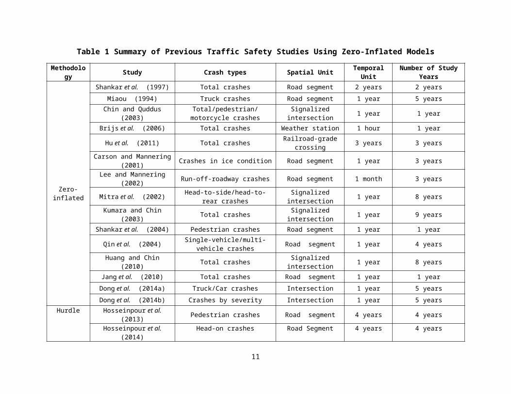
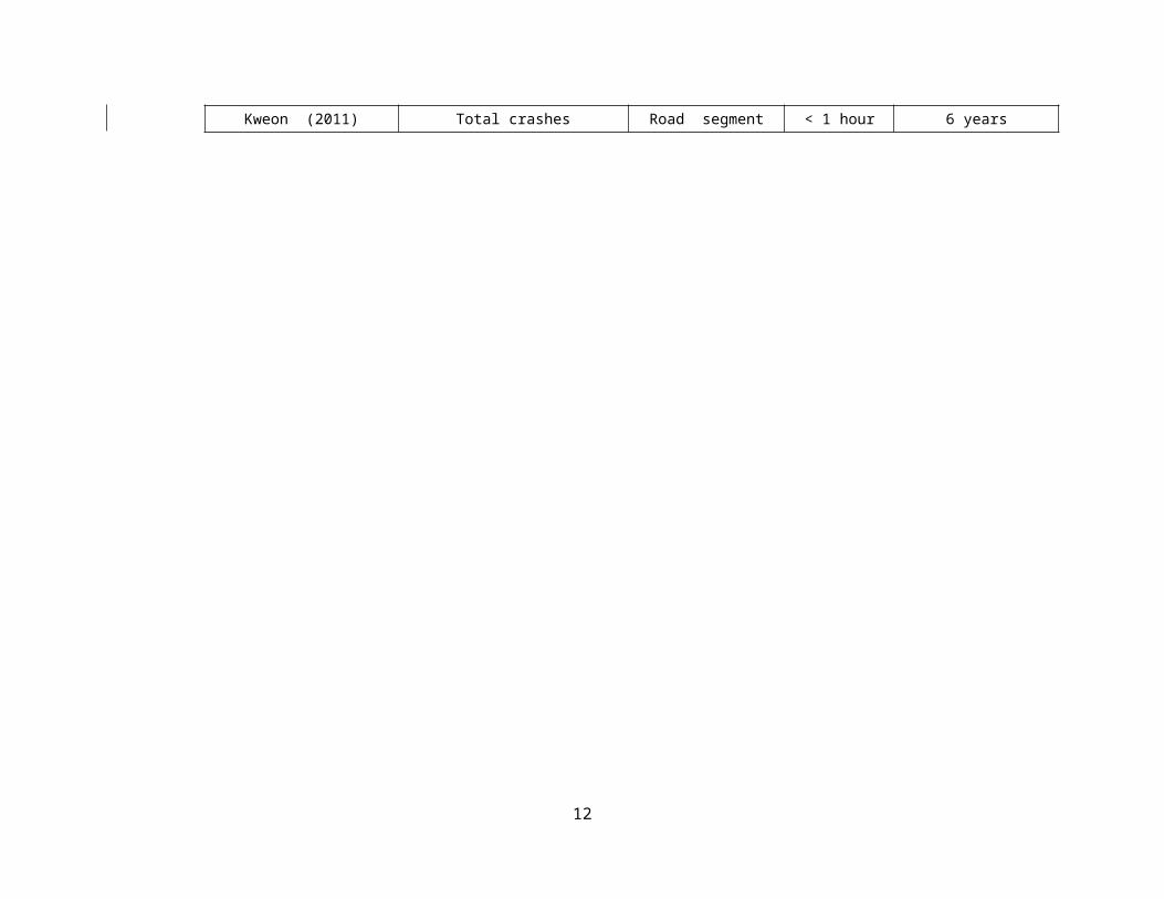
depend on the actual empirical dataset under consideration. Table 1 presents a summary of

previous studies that have considered zero-inflated and hurdle models to analyze crashes. The

table provides information on type and severity of crash analyzed, spatial and temporal unit of

analysis and the data collection duration. From the table, it is evident that all the existing zero-

inflated and hurdle studies are conducted at a micro-level such as segment and intersection

except for Brijs et al. (2006), which conducted crash analysis at macro-level by assigning

crashes to the closest weather station. Second, with the exception of study (Hu et al., 2011;

Hosseinpour et al., 2013; Hosseinpour et al., 2014), the range of observation of the study period

5

is one year or less; that may explain the preponderance of zeros in the data (Lord et al., 2005).

Third, the zero-inflated model always offers better statistical fit to crash data.

Issues with Dual-state Models

To be sure, several research studies have criticized the application of zero-inflated model for

traffic safety analysis (Lord et al., 2005; Lord et al., 2007; Kweon, 2011). The authors question

the basic dual-state assumption for crash occurrence and have conducted extensive analysis at

the micro-level and indicated that the development of models with dual-state process is

inconsistent with crash data at the micro-level. While the reasoning behind the “non-

applicability” is plausible for micro-level the reasoning does not necessarily carry over to the

macro-level crash counts. At the macro-level it is possible to visualize dual-state data generation

with some macro-level units having zero pedestrian and bicyclist crashes – possibly because

these spatial units have no pedestrian and bicycle demand (because of lack of walking and

cycling infrastructure). In such cases the dual-state representation will allow us to identify spatial

units that are likely to have zero cases as a function of exogenous variables (for example very

low walking and cycling infrastructure might result in the higher probability of a zero state).

Hence, we have considered the possible existence of dual-state models for pedestrian and bicycle

crashes at the macro level in our research. If the data generation does support the dual-state

models, ignoring the excess zeros and estimating traditional NB models will result in biased

estimates.

6

Table 1 Summary of Previous Traffic Safety Studies Using Zero-Inflated Models

Methodology Study Crash types Spatial Unit Temporal

UnitNumber of Study

Years

Zero-inflated

Shankar et al. (1997) Total crashes Road segment 2 years 2 years

Miaou (1994) Truck crashes Road segment 1 year 5 years

Chin and Quddus (2003) Total/pedestrian/motorcycle crashes Signalized intersection 1 year 1 year

Brijs et al. (2006) Total crashes Weather station 1 hour 1 year

Hu et al. (2011) Total crashes Railroad-grade crossing 3 years 3 years

Carson and Mannering (2001) Crashes in ice condition Road segment 1 year 3 years

Lee and Mannering (2002) Run-off-roadway crashes Road segment 1 month 3 years

Mitra et al. (2002) Head-to-side/head-to-rear crashes Signalized intersection 1 year 8 years

Kumara and Chin (2003) Total crashes Signalized intersection 1 year 9 years

Shankar et al. (2004) Pedestrian crashes Road segment 1 year 1 year

Qin et al. (2004) Single-vehicle/multi-vehicle crashes Road segment 1 year 4 years

Huang and Chin (2010) Total crashes Signalized intersection 1 year 8 years

Jang et al. (2010) Total crashes Road segment 1 year 1 year

Dong et al. (2014a) Truck/Car crashes Intersection 1 year 5 years

Dong et al. (2014b) Crashes by severity Intersection 1 year 5 years

Hurdle

Hosseinpour et al. (2013) Pedestrian crashes Road segment 4 years 4 years

Hosseinpour et al. (2014) Head-on crashes Road Segment 4 years 4 years

Kweon (2011) Total crashes Road segment < 1 hour 6 years

7

Spatial Spillover Effects

In macro-level analysis, crashes occurring in a spatial unit are aggregated to obtain the crash

frequency. The aggregation process might introduce errors in identifying the exogenous variables

for the spatial unit. For example, a crash occurring closer to the boundary of the unit might be

strongly related to the neighboring zone than the actual zone where the crash occurred. This is a

result of arbitrarily demarcating space. To accommodate for such spatial unit induced bias, two

approaches to incorporate spatial dependency are considered: (1) spatial error correlation effects

(unobserved exogenous variables at one location affect dependent variable at the targeted and

neighboring locations) and (2) spatial spillover effects (observed exogenous variables at one

location having impacts on the dependent variable at both the targeted and neighboring

locations) (Narayanamoorthy et al., 2013). Several research efforts have accommodated for

spatial random error in safety literature (for example see (Huang et al., 2010; Siddiqui et al.,

2012; Lee et al., 2015)). On the other hand, researchers have considered a spatially lagged

dependent variable at neighboring units for the spatial spillover effects (LaScala et al., 2000;

Quddus, 2008; Ha and Thill, 2011). However, the utility of such spatially lagged dependent

variable models, particularly for prediction, is limited since developing prediction frameworks

for spatially lagged models is involved. In our analysis, to accommodate for spatial effects, we

propose the consideration of exogenous variables from neighboring zones for accounting for

spatial dependency. The approach, referred to as spatial spillover model, is easy to implement

and allows practitioners to understand and quantify the influence of neighboring units on crash

frequency.

In summary, the current study contributes to non-motorized macro-level crash analysis along two

directions: (1) evaluate the viability of dual-state models for non-motorized crash analysis at

8

macro-level; and (2) introduction of spatial independent variables accounting for spatial spillover

effects on crash frequency. Towards this end, conventional single-state model (i.e., NB) and two

dual-state models (i.e., zero-inflated NB (ZINB) and hurdle NB (HNB)) with and without spatial

independent variables are developed for both pedestrian and bicycle crashes at a TAZ level in

Florida. Overall, both pedestrian and bicycle crashes have 6 model structures estimated - NB

model without/with spatial effects (aspatial/spatial NB), ZINB model without/with spatial effects

(aspatial/spatial ZINB), and HNB model without/with spatial effects (aspatial/spatial HNB). The

model development process considers a sample for model calibration and a hold-out sample for

validation. A comparison exercise is undertaken to identify the superior model in model

estimation and validation. Finally, average marginal effects are computed for the best model to

assess the effect of different factors, including the spatial variables on crash occurrence.

Methodology

Single-state models

The Poisson model is the traditional starting model for crash frequency analysis (Lord and

Mannering, 2010). The Poisson model assumes that the mean and variance of the distribution are

the same. Thus, the Poisson model cannot deal with the over-dispersion (i.e. variance exceeds the

mean). The NB model relaxes the equal mean variance assumption of Poisson model and allows

for over-dispersion parameter by adding an error term,ε i, to the mean of the Poisson model as:

λ i=exp ( β i x i+εi ) (1)

where λ i is the expected number of Poisson distribution for entity i , x i is a set of explanatory

variables, and β i is the corresponding parameter. Usually, exp (εi) is assumed to be gamma-

distributed with mean 1 and variance α so that the variance of the crash frequency distribution

9

becomes λ i(1+α λi) and different from the mean λ i. The NB model for the crash count y i of

entity i is given by

P( y i)=Г ( y i+

1α )

Г ( y i+1 ) Г ( 1α ) (

α λi

1+α λ i )y i

( 11+α λi

)1α (2)

where y i is the number of crashes y i of entity i and Г ( ∙ ) refers to the gamma function. The NB

model can generally account over-dispersion resulting from unobserved heterogeneity and

temporal dependency, but may be improper for accounting for the over-dispersion caused by

excess zero counts (Rose et al., 2006).

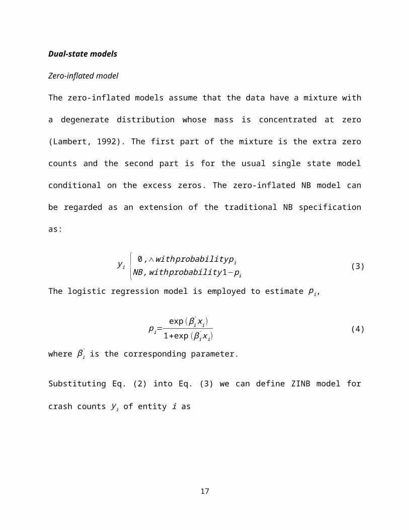
Dual-state models

Zero-inflated model

The zero-inflated models assume that the data have a mixture with a degenerate distribution

whose mass is concentrated at zero (Lambert, 1992). The first part of the mixture is the extra

zero counts and the second part is for the usual single state model conditional on the excess

zeros. The zero-inflated NB model can be regarded as an extension of the traditional NB

specification as:

y i { 0 ,∧with probability pi

NB , with probability1− pi(3)

The logistic regression model is employed to estimate pi,

pi=exp (β i

' x i)1+exp (βi

' x i)(4)

where β i' is the corresponding parameter.

10

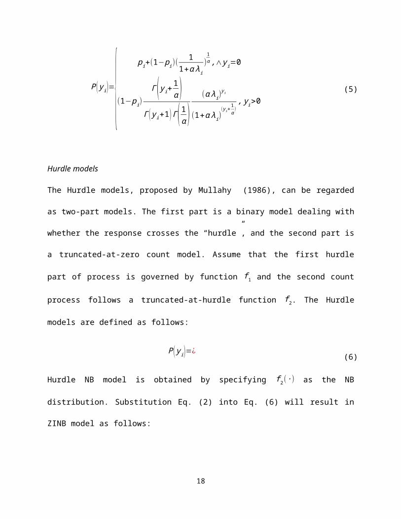
Substituting Eq. (2) into Eq. (3) we can define ZINB model for crash counts y i of entity i as

P ( y i )={ p i+(1−p i)(1

1+α λ i)

1α ,∧ y i=0

(1−pi)Г ( y i+

1α )

Г ( y i+1 ) Г ( 1α )

(α λ i)y i

(1+α λ i)( yi +

1α )

, y i>0(5)

Hurdle models

The Hurdle models, proposed by Mullahy (1986), can be regarded as two-part models. The first

part is a binary model dealing with whether the response crosses the “hurdle”, and the second

part is a truncated-at-zero count model. Assume that the first hurdle part of process is governed

by function f 1 and the second count process follows a truncated-at-hurdle function f 2. The

Hurdle models are defined as follows:

P ( yi )=¿(6)

Hurdle NB model is obtained by specifying f 2(∙) as the NB distribution. Substitution Eq. (2) into

Eq. (6) will result in ZINB model as follows:

P ( yi )={p i ,∧ y i=0

(1−pi)(1−1

(1+α λi)1α

)Г ( yi+

1α )

Г ( y i+1 ) Г ( 1α )

(α λi)y i

(1+α λi)(y i+

1α

), y i>0 (7)

As in the zero-inflated model, logistic regression will be applied for modeling pi.

Data Preparation

11

About 16,240 pedestrian and 15,307 bicycle involved crashes that occurred in Florida in the

period of 2010-2012 were compiled for the analysis. The State of Florida has 8,518 TAZs, with

an average area of 6.472 square miles. This TAZ system used in this paper is developed and used by

the Florida Department of Transportation Central Office for statewide level transportation planning.

Among the TAZs, as shown in Figure 1, 46.18% of them have zero pedestrian crashes while

49.86% of them didn’t have any bicycle crashes. The explanatory variables considered for the

analysis can be grouped into three categories: traffic (such as VMT (Vehicle-Miles-Traveled),

proportion of heavy vehicle in VMT), roadway (such as signalized intersection density, length of

bike lanes and sidewalks, etc.), and socio-demographic characteristics (such as population

density, proportion of families without vehicle, etc.).

As highlighted earlier, the current analysis focuses on accommodating the impact of neighboring

TAZs on the crash frequency models. Towards this end, for every TAZ, the TAZs that are

adjacent are identified. Based on the identified neighbors, a new variable based on the value of

the each exogenous variable from surrounding TAZs is computed. The variables thus created

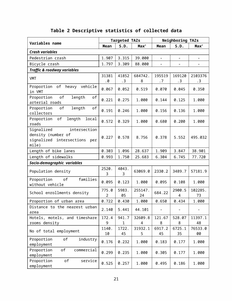
capture the spatial spillover effects of the neighboring TAZs on crash frequency. The descriptive

statistics of the crash counts and independent variables are summarized in Table 2. Specifically,

the table provides the values at a TAZ level as well as for the neighboring TAZ variables.

12

Table 2 Descriptive statistics of collected data

Variables nameTargeted TAZs Neighboring TAZs

Mean S.D. Maxa Mean S.D. Maxa

Crash variablesPedestrian crash 1.907 3.315 39.000 - - -Bicycle crash 1.797 3.309 88.000 - - -Traffic & roadway variables

VMT 31381.0 41852.3 684742.8 195519.7 169120.

3 2103376.3

Proportion of heavy vehicle in VMT 0.067 0.052 0.519 0.070 0.045 0.350Proportion of length of arterial roads 0.221 0.275 1.000 0.144 0.125 1.000Proportion of length of collectors 0.191 0.246 1.000 0.156 0.136 1.000Proportion of length local roads 0.572 0.329 1.000 0.680 0.200 1.000Signalized intersection density (number of signalized intersections per mile) 0.227 0.578 8.756 0.378 5.552 495.032

Length of bike lanes 0.303 1.096 28.637 1.909 3.847 38.901Length of sidewalks 0.993 1.750 25.683 6.304 6.745 77.720Socio-demographic variablesPopulation density 2520.3 4043.3 63069.0 2330.2 3489.7 57181.9Proportion of families without vehicle 0.095 0.123 1.000 0.095 0.108 1.000School enrollments density 775.02 5983.05 255147.24 684.22 2900.54 102285.73Proportion of urban area 0.722 0.430 1.000 0.650 0.434 1.000Distance to the nearest urban area 2.140 5.441 44.101 - - -Hotels, motels, and timeshare rooms density 172.49 941.71 32609.84 121.678 528.078 11397.148

No of total employment 1140.10 1722.45 31932.15 6917.245 6725.13

5 76533.000

Proportion of industry employment 0.176 0.232 1.000 0.183 0.177 1.000Proportion of commercial employment 0.299 0.235 1.000 0.305 0.177 1.000Proportion of service employment 0.525 0.257 1.000 0.495 0.186 1.000No of commuters by public transportation 18.813 54.273 934.000 119.582 246.299 3559.985No of commuters by cycling 5.894 19.804 775.000 90.869 128.399 1902.135No of commuters by walking 14.354 34.680 1288.000 37.566 74.484 1634.530

a The minimum values for all variables are zero.

13

Figure 1 Pedestrian and bicycle crashes based on TAZs

Modeling Results and Discussion

Goodness of fit

In this study, from the 8518 TAZs, 80% of the zones were randomly selected for models

calibration and 20% were used for validation of the estimated models. The overall model

estimation process involved estimating six models - 3 model types (NB, ZINB, and HNB

models) with and without spatial independent variables of neighboring TAZs for pedestrian and

bicycle crashes. Prior to discussing the model results, we present the goodness of fit measures of

the estimated models in Table 3. The table presents the Log-likelihood, Akaike Information

Criterion (AIC) and Bayesian Information Criterion (BIC) - for the 6 models for estimation and

validation samples. Several observations can be made from the results presented in Table 3.

First, across pedestrian and bicycle crash models, the models with spatial independent variables

offer substantially better fit compared to models without spatial independent variables. The

results validate our hypothesis that characteristics of adjacent TAZs improve our understanding

14

of crash frequency in the target TAZ. Second, the exact ordering alters between ZINB and HNB

in some cases based on log-likelihood and AIC. However, the ZINB model offers the best fit

across all model structures based on the BIC. Among aspatial and spatial models, the ZINB

model always has the lowest BIC value indicating strong difference between ZINB and other

models. The ZINB improves data fit with only a small increase in number of parameters. Hence,

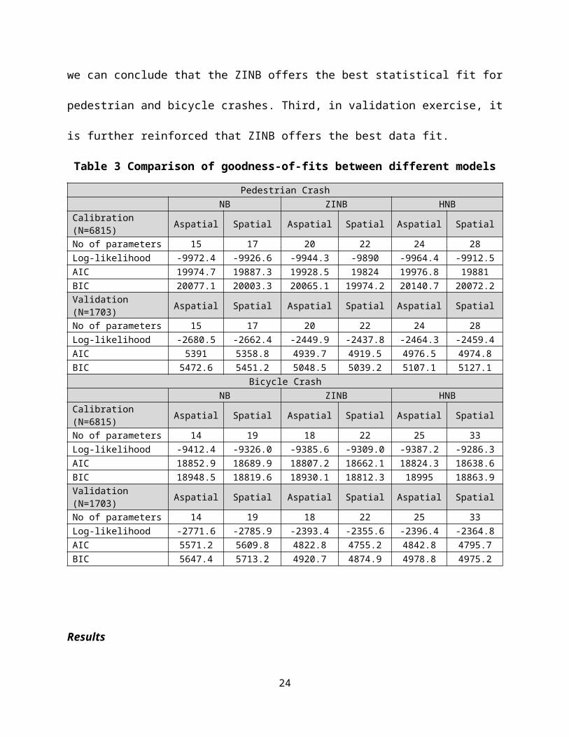
in terms of our results, we can conclude that the ZINB offers the best statistical fit for pedestrian

and bicycle crashes. Third, in validation exercise, it is further reinforced that ZINB offers the

best data fit.

Table 3 Comparison of goodness-of-fits between different models

Pedestrian CrashNB ZINB HNB

Calibration (N=6815) Aspatial Spatial Aspatial Spatial Aspatial SpatialNo of parameters 15 17 20 22 24 28Log-likelihood -9972.4 -9926.6 -9944.3 -9890 -9964.4 -9912.5AIC 19974.7 19887.3 19928.5 19824 19976.8 19881BIC 20077.1 20003.3 20065.1 19974.2 20140.7 20072.2Validation (N=1703) Aspatial Spatial Aspatial Spatial Aspatial SpatialNo of parameters 15 17 20 22 24 28Log-likelihood -2680.5 -2662.4 -2449.9 -2437.8 -2464.3 -2459.4AIC 5391 5358.8 4939.7 4919.5 4976.5 4974.8BIC 5472.6 5451.2 5048.5 5039.2 5107.1 5127.1

Bicycle CrashNB ZINB HNB

Calibration (N=6815) Aspatial Spatial Aspatial Spatial Aspatial SpatialNo of parameters 14 19 18 22 25 33Log-likelihood -9412.4 -9326.0 -9385.6 -9309.0 -9387.2 -9286.3AIC 18852.9 18689.9 18807.2 18662.1 18824.3 18638.6BIC 18948.5 18819.6 18930.1 18812.3 18995 18863.9Validation (N=1703) Aspatial Spatial Aspatial Spatial Aspatial SpatialNo of parameters 14 19 18 22 25 33Log-likelihood -2771.6 -2785.9 -2393.4 -2355.6 -2396.4 -2364.8AIC 5571.2 5609.8 4822.8 4755.2 4842.8 4795.7BIC 5647.4 5713.2 4920.7 4874.9 4978.8 4975.2

15

Results

The results of six models (3 model types with and without spatial independent variables of

neighboring TAZs) for pedestrian and bicycle crashes each are displayed in Table 4 and Table 5

separately. The results for NB models only have the count frequency component. For zero-

inflated and hurdle models, the modeling results consist of two components: (1) logistic model

component for zero state and (2) the count frequency component. Across the 6 models for either

pedestrian or bicycle crashes, the significant variables are different. Some of the explanatory

variables such as VMT, population density are transformed into the natural logarithmic scale.

Generally, a log link between dependent and independent variables is specified in the modeling

regression. Thus, with the transformation of the independent variables, the relationship of power

function between explanatory variables and crash counts can be obtained which was widely

adopted in previous research (Greibe, 2003; Abbas, 2004). Also, this transformation reduces

variance and minimize the heteroscedasticity among the variables (Quddus, 2008; Gujarati,

2012). Meanwhile, with a log transformation the parameter of the explanatory variable results in

a linear elasticity which is easy to interpret. While the results for all models for pedestrians and

bicycle crashes are presented, the discussion focuses on the ZINB model with spatial

independent variables that offers the best fit.

Pedestrian crash models for TAZs

For ZINB model with spatial independent variables, twelve independent variables of targeted

TAZs and four spatial independent variables are significant in the count component.

16

The VMT variable is a measure of vehicle exposure and as expected increases the propensity for

pedestrian crashes. However, with increase in heavy vehicle VMT, TAZs are likely to have

lower pedestrian exposure resulting in lower probability of vehicle-pedestrian interactions.

Population density and total employment variables are surrogate measures of pedestrian

exposure (Siddiqui et al., 2012). Hence, it is expected that these variables have positive impacts

on crash frequency. The variables proportion of local roads by length, signalized intersection

density, and length of sidewalks are reflections of pedestrian access. Increased local roads,

signalized intersections, and sidewalks may attract more pedestrians and are likely to increase

crash frequency. The positive estimate of the number of hotels, motels and timeshare rooms’

variable reflects land use characteristics that are likely to encourage walking in the vicinity

increasing pedestrian exposure. It is observed that in TAZs with higher number of commuters by

walking and public transportation, the propensity for pedestrian crashes is higher. The

commuters by walking and public transportation reflect zones with higher pedestrian activity

resulting in increased crash risk (Abdel-Aty et al., 2013). As the distance from a TAZ geometric

centroid to the nearest urban region increases, pedestrian crash risk in the TAZ reduces – a sign

of low pedestrian activity in the suburban regions.

Among the significant spatial spillover variables, the proportion of service employment

corresponds to surrounding land use characteristics that attract pedestrians and therefore

increases the propensity of pedestrian crashes. Interestingly, the impact of signalized intersection

density of neighboring TAZs is found to be negatively associated with pedestrian crash

frequency. This result is in contrast to the impact of the same variable for the targeted TAZ. The

number of signalized intersections reflects the increase in exposure for pedestrians thus resulting

in an increase in crashes. However, the influence of signalized intersections in neighboring TAZs

17

has an ameliorating impact on crash frequency i.e., TAZs surrounded by zones with higher

signalized intersection density have a lower propensity for crash occurrence because the higher

density of signalized intersections is likely to increase driver awareness of pedestrians offsetting

the exposure effect marginally (Zajac and Ivan, 2003; Eluru et al., 2008). The proportion of families

without vehicles in the vicinity of TAZ represents captive individuals that are forced to use

public transit and pedestrian/bicycle modes. Thus increased presence of such families is likely to

increase pedestrian exposure, leading to more pedestrian crashes. Higher number of commuters

by public transportation in the neighboring TAZs also results in increased pedestrian crash

frequency.

In the probabilistic component, only the length of sidewalks, number of total employment, and

number of commuters by public transportation of the targeted TAZs are significant. As expected,

these three variables are negatively associated with the propensity of zero pedestrian crashes. As

these variables serve as surrogates for pedestrian activity, it is expected that TAZs with higher

levels of these variables are unlikely to be assigned to the zero crash state. Interestingly, no

spatial spillover effects are found to be significant in the probabilistic part.

18

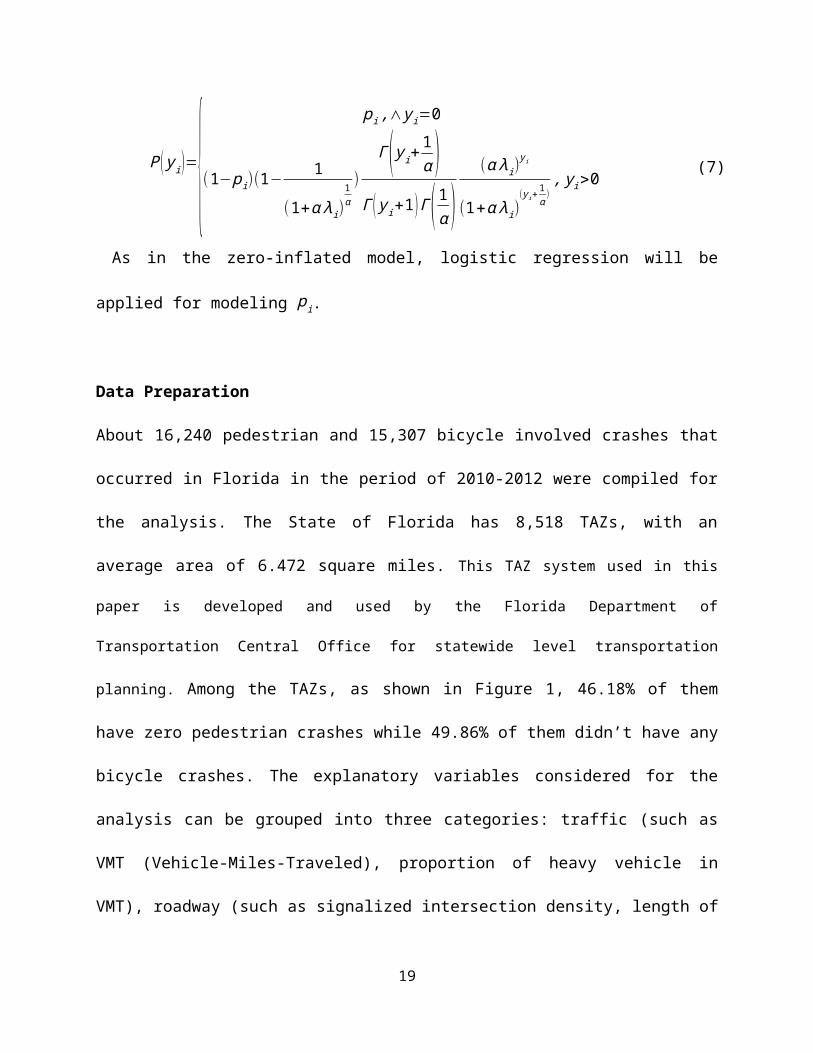
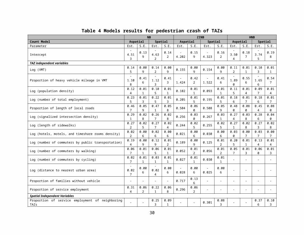
Table 4 Models results for pedestrian crash of TAZsNB ZINB HNB

Count Model Aspatial Spatial Aspatial Spatial Aspatial SpatialParameter Est. S.E. Est. S.E. Est. S.E. Est. S.E. Est. S.E. Est. S.E.Intercept -4.513 0.139 -4.632 0.142 -4.202 0.159 -4.323 0.162 -3.504 0.187 -3.745 0.198TAZ independent variablesLog (VMT) 0.145 0.009 0.142 0.009 0.155 0.009 0.154 0.009 0.112 0.011 0.103 0.011Proportion of heavy vehicle mileage in VMT -1.108 0.416 -1.123 0.413 -1.424 0.422 -1.522 0.416 -1.890 0.556 -1.656 0.547Log (population density) 0.124 0.011 0.105 0.011 0.102 0.011 0.093 0.011 0.115 0.014 0.097 0.014Log (number of total employment) 0.235 0.013 0.225 0.013 0.205 0.015 0.195 0.015 0.186 0.017 0.186 0.017Proportion of length of local roads 0.467 0.059 0.471 0.058 0.504 0.060 0.508 0.059 0.480 0.080 0.454 0.080Log (signalized intersection density) 0.291 0.028 0.267 0.028 0.256 0.030 0.267 0.031 0.274 0.038 0.286 0.040Log (length of sidewalks) 0.272 0.025 0.277 0.024 0.244 0.025 0.255 0.025 0.271 0.028 0.273 0.028Log (hotels, motels, and timeshare rooms density) 0.022 0.006 0.026 0.006 0.021 0.006 0.030 0.006 0.030 0.007 0.037 0.007Log (number of commuters by public transportation) 0.194 0.009 0.129 0.012 0.189 0.009 0.125 0.012 0.205 0.011 0.134 0.014Log (number of commuters by walking) 0.067 0.011 0.065 0.011 0.052 0.012 0.056 0.012 0.057 0.013 0.060 0.013Log (number of commuters by cycling) 0.027 0.011 0.031 0.011 0.027 0.011 0.030 0.011 - - - -Log (distance to nearest urban area) -0.027 0.006 -0.024 0.006 -0.028 0.006 -0.025 0.006 - - - -Proportion of families without vehicle - - - - 0.717 0.136 - - - - - -Proportion of service employment 0.314 0.062 0.221 0.068 0.296 0.062 - - - - - -Spatial Independent VariablesProportion of service employment of neighboring TAZs - - 0.253 0.091 - - 0.301 0.083 - - 0.376 0.103Log (signalized intersection density of neighboring TAZs) - - - - - - -0.291 0.063 - - -0.211 0.073Proportion of families without vehicle of neighboring TAZs - - - - - - 1.29 0.172 - - - -Log (number of commuters by public transportation of neighboring TAZs) - - 0.099 0.011 - - 0.091 0.011 - - 0.108 0.014Dispersion 0.445 0.020 0.423 0.020 0.393 0.022 0.367 0.021 0.419 0.028 0.386 0.026Probabilistic Model Aspatial Spatial Aspatial Spatial Aspatial SpatialIntercept - - - - 0.070 0.413 -0.047 0.431 5.733 0.237 5.791 0.238TAZ independent variablesLog (VMT) - - - - - - - - -0.188 0.015 -0.184 0.015Log (length of sidewalks) - - - - -2.143 0.729 -1.995 0.715 -0.500 0.064 -0.502 0.064Log (number of total employment) - - - - -0.240 0.070 -0.232 0.072 -0.299 0.023 -0.295 0.023Log (number of commuters by walking) - - - - -0.527 0.153 -0.501 0.148 -0.138 0.027 -0.136 0.027Proportion of length of local roads - - - - - - - - -0.510 0.104 -0.516 0.104Log (signalized intersection density) - - - - - - - - -0.331 0.054 -0.319 0.054Log (population density) - - - - - - - - -0.164 0.019 -0.155 0.019Proportion of service employment - - - - - - - - -0.405 0.126 -0.413 0.127Log (number of commuters by public transportation) - - - - -0.247 0.025 -0.192 0.030Log (number of commuters by cycling) - - - - - - - - -0.074 0.032 -0.074 0.032Log (distance to nearest urban area) - - - - - - - - 0.030 0.008 0.027 0.008Spatial Independent VariablesLog (number of commuters by public transportation of neighboring TAZs) - - - - - - - - - - -0.075 0.022

All explanatory variables are significant at 95% confidence level

19

Bicycle crash models for TAZs

In the ZINB model with spatial variables presented in Table 5 eleven variables for the TAZs and

five variables of neighboring TAZs affect bicycle crash frequency. The impacts of exogenous

variables in the bicycle crash frequency model are very similar to the impact of these variables in

the pedestrian crash frequency model. This is not surprising because, TAZs that are likely to

experience high pedestrian activity are also likely to experience high bicyclist activity.

For the count component, the exogenous variables for the TAZ that increase the crash propensity

are VMT, population density, total employment, proportion of local roads by length, signalized

intersection density, length of sidewalks, proportion of commuters by walking as well as cycling,

and proportion of service employment. The exogenous variables for the TAZ that reduce crash

propensity are proportion of heavy vehicle mileage and the distance of the TAZ centroid from

the nearest urban region. There are three main difference in the TAZ variable impacts between

pedestrian and bicyclist crash frequency. First, the number of commuters by public transportation

does not have significant impacts on crash frequency as it is possible that public transportation

and bicycling are not as strongly correlated as is the case with public transportation and

pedestrians. Second, the density of hotel, motel and time share rooms does not impact bicycle

crash frequency as tourists are less likely to be bicyclists. Third, the service employment count in

the TAZ affects bicycle crash frequency while affecting pedestrian crash frequency as a spillover

effect. While, the exact reason for the result is unclear, it could be a manifestation of differences

of how land-use affects pedestrians and bicyclists.

In terms of spatial spillover effects, the significant variables vary between pedestrian and

bicyclists. Specifically, the high proportion of industry employment in neighboring TAZs has a

negative association with crash propensity indicating that surrounding regions especially the

20

targeted TAZs are unlikely to have significant bicyclist exposure. The signalized intersection

density exhibits the same relationship as described for pedestrian crashes. On the other hand,

from the neighboring TAZs, population density, number of commuters by public transit and

cycling are surrogates for bicyclist exposure and are found positively associated with bicycle

crashes.

In the probabilistic component, only three explanatory variables of targeted TAZs variables are

significant. The length of sidewalks, population density and total employment variables, as

expected, have negative influence on assigning a TAZ to a zero crash state. The bicycle crash

probabilistic component also does not have any statistically significant spatial variables.

21

Table 5 Models results for bicycle crash of TAZsNB ZINB HNB

Count Model Aspatial  Spatial Aspatial Spatial Aspatial SpatialParameter Est. S.E. Est. S.E. Est. S.E. Est. S.E. Est. S.E. Est. S.E.Intercept -4.650 0.154 -4.672 0.167 -4.090 0.181 -4.673 0.190 -3.620 0.220 -4.031 0.237TAZ independent variablesLog (VMT) 0.190 0.009 0.162 0.010 0.186 0.010 0.164 0.010 0.168 0.013 0.148 0.013Proportion of heavy vehicle mileage in VMT -4.260 0.485 -3.306 0.490 -4.244 0.487 -2.787 0.496 -4.115 0.665 -2.949 0.660Log (population density) 0.152 0.013 0.130 0.013 0.133 0.014 0.087 0.015 0.131 0.018 0.084 0.020Log (number of total employment) 0.193 0.014 0.194 0.014 0.157 0.016 0.161 0.016 0.142 0.018 0.134 0.018Proportion of length of local roads 0.535 0.062 0.441 0.064 0.517 0.063 0.525 0.063 0.422 0.086 0.401 0.085Log (signalized intersection density) 0.196 0.030 0.234 0.032 0.172 0.031 0.203 0.033 0.125 0.041 0.184 0.044Log (length of sidewalks) 0.284 0.026 0.271 0.025 0.214 0.027 0.228 0.026 0.219 0.030 0.217 0.029Log (number of commuters by public transportation) 0.106 0.010 0.086 0.012 0.107 0.010 - - 0.096 0.012 0.084 0.012Log (number of commuters by walking) 0.087 0.012 0.085 0.012 0.090 0.012 0.104 0.012 0.101 0.014 0.099 0.014Log (number of commuters by cycling) 0.109 0.011 0.070 0.012 0.110 0.011 0.088 0.012 0.108 0.012 0.071 0.013Log (distance to nearest urban area) -0.103 0.011 -0.098 0.011 -0.097 0.011 -0.074 0.011 -0.092 0.024 -0.065 0.023Proportion of service employment 0.205 0.066 0.153 0.067 0.192 0.066 0.173 0.067 - - - -Spatial Independent VariablesProportion of industry employment of neighboring TAZs - - -0.361 0.106 - - -0.242 0.106 - - - -Log (signalized intersection density of neighboring TAZs) - - -0.319 0.075 - - -0.473 0.069 - - -0.545 0.095Log (population density of neighboring TAZs) - - - - - - 0.113 0.018 - - 0.109 0.023Log (number of commuters by public transportation of neighboring TAZs) - - 0.035 0.012 - - 0.068 0.010 - - - -Log (number of commuters by cycling of neighboring TAZs) - - 0.093 0.012 - - 0.073 0.012 - - 0.098 0.014Proportion of length of local roads of neighboring TAZs - - 0.354 0.125 - - - - - - - -Dispersion 0.481 0.022 0.443 0.021 0.425 0.022 0.397 0.021 0.454 0.031 0.406 0.028Probabilistic Model Aspatial Spatial Aspatial Spatial Aspatial  SpatialIntercept - - - - 1.565 0.489 1.296 0.509 5.452 0.241 5.700 0.279TAZ independent variablesLog (VMT) - - - - - - - - -0.222 0.016 -0.217 0.017Log (length of sidewalks) - - - - -4.455 1.272 -4.819 1.563 -0.676 0.066 -0.681 0.066Log (population density) - - - - -0.149 0.05 -0.135 0.053 -0.177 0.021 -0.102 0.024Log (number of total employment) - - - - -0.328 0.058 -0.313 0.060 -0.236 0.023 -0.216 0.024Proportion of heavy vehicle mileage in VMT - - - - - - - - 5.347 0.836 4.258 0.861Proportion of length of local roads - - - - - - - - -0.709 0.109 -0.696 0.112Log (signalized intersection density) - - - - - - - - -0.286 0.054 -0.243 0.056Log (number of commuters by public transportation) - - - - - - - - -0.210 0.025 -0.147 0.031Log (number of commuters by walking) - - - - - - - - -0.081 0.028 -0.079 0.028Log (number of commuters by cycling) - - - - - - - - -0.158 0.032 -0.099 0.035Log (distance to nearest urban area) - - - - - - - - 0.098 0.013 0.082 0.013Spatial Independent VariablesProportion of length of arterial of neighboring TAZs - - - - - - - - - - 1.337 0.290Log (population density of neighboring TAZs) - - - - - - - - - - -0.096 0.033Log (hotels, motels, and timeshare rooms density of neighboring TAZs) - - - - - - - - - - -0.041 0.018Log (number of commuters by public transportation of neighboring TAZs) - - - - - - - - - - -0.069 0.026Log (number of commuters by cycling of neighboring TAZs) - - - - - - - - - - -0.082 0.025

22

All explanatory variables are significant at 95% confidence level

Marginal effects

The ZINB has two components, the probabilistic and the count component with exogenous

variables possibly affecting both components. Thus, it is not straight-forward to identify the

exact magnitude of the variable impact. Hence, to facilitate a quantitative comparison of variable

impacts, marginal effects for the ZINB for pedestrians and bicyclists are computed. The marginal

effects capture the change in the dependent variable in response to a small change in the

independent variables. The results of the marginal effect calculation are presented in Table 6. As

is expected, the sign of the marginal effects closely follows the sign from model results described

in Table 4 and 5. The marginal effects represent the percentage change in the crash frequency

variable for a 1% change in the exogenous variable. For example, for the first row in Table 6, a

1% change in Log(VMT) is likely to result in a 0.292% change in pedestrian crash frequency and

0.291% change in bicyclist crash frequency. The other parameters can also be interpreted in a

similar fashion.

The following observations can be made based on the results presented. First, the impact of

spatial spillover effects on the crash models is significant and is comparable to the influence of

other exogenous variables. Hence, it is important that analysts consider such observed spatial

spillover effects in crash frequency modeling. Second, the exogenous variable impacts on

pedestrian and bicycle crash models are similar for a large number of variables including VMT,

population density, total employment, number of commuters by walking, proportion of local

road in length, and number of public transportation commuters in neighboring TAZs. All of these

variables have marginal effects with positive values, indicating number of crashes (for both

pedestrian and bicycle crashes) increase as these variables increase. Third, the exogenous

variables such as proportion of heavy vehicle VMT, proportion of service employment, number

23

of commuters by public transportation and cycling, proportion of families without vehicles in the

neighboring TAZs, service employment and industry employment in neighboring TAZs have

significantly different marginal impacts across the two models. Their negative marginal effect

values show that crash counts will decrease if these variables increase. Finally, as indicated by

the marginal effects of the signalized intersection density the exogenous variable for TAZ and

neighboring TAZs could exhibit distinct effects both in sign and magnitude. The allowance of

such non-linear impacts accommodates for heterogeneity in the data.

Table 6 Average marginal effect for ZINB model with spatial independent variables

Pedestrian Bicycle Variables dy/dx S.E dy/dx S.ETAZ independent variablesLog (VMT) 0.292 0.018 0.291 0.018Proportion of heavy vehicle mileage in VMT -2.888 0.791 -4.937 0.885Log (population density) 0.176 0.021 0.162 0.027Log (number of total employment) 0.382 0.027 0.302 0.027Proportion of length of local roads 0.965 0.114 0.930 0.113Log (signalized intersection density) 0.506 0.06 0.359 0.059Log (length of sidewalks) 0.587 0.05 0.671 0.077Log (hotels, motels, and timeshare rooms density) 0.056 0.011 - -Log (number of commuters by public transportation) 0.238 0.022 - -Log (number of commuters by walking) 0.131 0.021 0.184 0.021Log (number of commuters by cycling) 0.057 0.02 0.156 0.021Log (distance to nearest urban area) -0.047 0.011 -0.132 0.019Proportion of service employment - - 0.307 0.118

Spatial Independent VariablesProportion of service employment of neighboring TAZs 0.572 0.158 - -Proportion of industry employment of neighboring TAZs - - -0.428 0.189Log (signalized intersection density of neighboring TAZs) -0.552 0.119 -0.838 0.124Proportion of families without vehicle of neighboring T AZs 2.447 0.329 - -Log (population density of neighboring TAZs) - - 0.200 0.033Log (number of commuters by public transportation of neighboring TAZs) 0.173 0.021 0.120 0.019

Log (number of commuters by cycling of neighboring TAZs) - - 0.130 0.021

24

Conclusion

With growing concern of global warming and obesity concerns, active forms of transportation

offer an environmentally friendly and physically active alternative for short distance trips. A

strong impediment to universal adoption of active forms of transportation, particularly in North

America, is the inherent safety risk for active modes of transportation. Towards developing

counter measures to reduce safety risks, it is essential to study the influence of exogenous factors

on pedestrian and bicycle crashes. This study contributes to safety literature by conducting a

macro-level planning analysis for pedestrian and bicycle crashes at a Traffic Analysis Zone

(TAZ) level in Florida. The study considers dual-state count models (zero-inflated negative

binomial (ZINB) and hurdle negative binomial (HNB)) for analysis by comparing with classical

single state (negative binomial (NB)) and. In addition to the dual-state models, the research

proposes the consideration of spatial spillover effects of exogenous variables from neighboring

TAZs. The model development exercise involved estimating 6 model structures each for

pedestrians and bicyclists. These include NB model with and without spatial effects, ZINB

model with and without spatial effects and HNB with and without spatial effects. The estimated

model performance was evaluated for the calibration sample and the validation sample using the

following measures: Log-likelihood, Akaike Information Criterion and Bayesian Information

Criterion.

The model comparison exercise for pedestrians and bicyclists highlighted that models with

spatial spillover effects consistently outperformed the models that did not consider the spatial

effects. Across the three models with spatial spillover effects, the ZINB model offered the best

fit for pedestrian and bicyclists. The model results clearly highlighted the importance of several

variables including traffic (such as VMT and heavy vehicle mileage), roadway (such as

25

signalized intersection density, length of sidewalks and bike lanes, and etc.) and socio-

demographic characteristics (such as population density, commuters by public transportation,

walking and cycling) of the targeted and neighboring TAZs. To facilitate a quantitative

comparison of variable impacts, marginal effects for the ZINB for pedestrians and bicyclists are

computed. The results revealed the importance in sign and magnitude of the spatial spillover

effect relative to other exogenous variables. Further, the marginal effects computation allowed us

to identify factors that substantially increase crash risk for pedestrians and bicyclists. In terms of

actionable information, it is important to identify zones with high public transit, pedestrian and

bicyclist commuters and undertake infrastructure improvements to improve safety.

To be sure, the study is not without limitations. While the influence of spatial spillover effects is

considered, we do not consider the impact of spatial unobserved effects. Extending the current

approach to accommodate for unobserved spatial terms will be useful. In this study, we

considered the distance from urban centers to the TAZ centroids determined purely based on the

physical characteristics. It would be useful to consider TAZ centroids based on activity facilities.

Also, it is possible to hypothesize that there might be common unobserved factors that affect

pedestrian and bicyclists. Future research extensions might consider such unobserved effects in

the model structure.

Acknowledgments

The authors would like to thank the Florida Department of Transportation (FDOT) for funding

this study.

26

Reference

Abbas, K.A., 2004. Traffic safety assessment and development of predictive models for accidents on rural roads in egypt. Accident Analysis & Prevention 36 (2), 149-163.

Abdel-Aty, M., Lee, J., Siddiqui, C., Choi, K., 2013. Geographical unit based analysis in the context of transportation safety planning. Transportation Research Part A: Policy and Practice 49, 62-75.

Abdel-Aty, M.A., Radwan, A.E., 2000. Modeling traffic accident occurrence and involvement. Accident Analysis & Prevention 32 (5), 633-642.

Aguero-Valverde, J., Jovanis, P.P., 2008. Analysis of road crash frequency with spatial models. Transportation Research Record: Journal of the Transportation Research Board 2061 (1), 55-63.

Brijs, T., Offermans, C., Hermans, E., Stiers, T., Year. Impact of weather conditions on road safety investigated on hourly basis. In: Proceedings of the Transportation Research Board 85th Annual Meeting.

Carson, J., Mannering, F., 2001. The effect of ice warning signs on ice-accident frequencies and severities. Accident Analysis & Prevention 33 (1), 99-109.

Cheng, L., Geedipally, S.R., Lord, D., 2013. The poisson–weibull generalized linear model for analyzing motor vehicle crash data. Safety science 54, 38-42.

Chin, H.C., Quddus, M.A., 2003. Modeling count data with excess zeroes an empirical application to traffic accidents. Sociological methods & research 32 (1), 90-116.

Dong, C., Clarke, D.B., Yan, X., Khattak, A., Huang, B., 2014a. Multivariate random-parameters zero-inflated negative binomial regression model: An application to estimate crash frequencies at intersections. Accid Anal Prev 70, 320-9.

Dong, C., Richards, S.H., Clarke, D.B., Zhou, X., Ma, Z., 2014b. Examining signalized intersection crash frequency using multivariate zero-inflated poisson regression. Safety Science 70, 63-69.

Eluru, N., Bhat, C.R., Hensher, D.A., 2008. A mixed generalized ordered response model for examining pedestrian and bicyclist injury severity level in traffic crashes. Accident Analysis & Prevention 40 (3), 1033-1054.

Greibe, P., 2003. Accident prediction models for urban roads. Accident Analysis & Prevention 35 (2), 273-285.

Gujarati, D.N., 2012. Basic econometrics Tata McGraw-Hill Education.

Ha, H.-H., Thill, J.-C., 2011. Analysis of traffic hazard intensity: A spatial epidemiology case study of urban pedestrians. Computers, Environment and Urban Systems 35 (3), 230-240.

27

Hosseinpour, M., Prasetijo, J., Yahaya, A.S., Ghadiri, S.M.R., 2013. A comparative study of count models: Application to pedestrian-vehicle crashes along malaysia federal roads. Traffic injury prevention 14 (6), 630-638.

Hosseinpour, M., Yahaya, A.S., Sadullah, A.F., 2014. Exploring the effects of roadway characteristics on the frequency and severity of head-on crashes: Case studies from malaysian federal roads. Accident Analysis & Prevention 62, 209-222.

Hu, S.-R., Li, C.-S., Lee, C.-K., 2011. Assessing casualty risk of railroad-grade crossing crashes using zero-inflated poisson models. Journal of Transportation Engineering 137 (8), 527-536.

Huang, H., Abdel-Aty, M., Darwiche, A., 2010. County-level crash risk analysis in florida: Bayesian spatial modeling. Transportation Research Record: Journal of the Transportation Research Board (2148), 27-37.

Huang, H., Chin, H.C., 2010. Modeling road traffic crashes with zero-inflation and site-specific random effects. Statistical Methods & Applications 19 (3), 445-462.

Jang, H., Lee, S., Kim, S.W., 2010. Bayesian analysis for zero-inflated regression models with the power prior: Applications to road safety countermeasures. Accid Anal Prev 42 (2), 540-7.

Kumara, S.S., Chin, H.C., 2003. Modeling accident occurrence at signalized tee intersections with special emphasis on excess zeros. Traffic Inj Prev 4 (1), 53-7.

Kweon, Y.-J., 2011. Development of crash prediction models with individual vehicular data. Transportation research part C: emerging technologies 19 (6), 1353-1363.

Lambert, D., 1992. Zero-inflated poisson regression, with an application to defects in manufacturing. Technometrics 34 (1), 1-14.

Lascala, E.A., Gerber, D., Gruenewald, P.J., 2000. Demographic and environmental correlates of pedestrian injury collisions: A spatial analysis. Accident Analysis & Prevention 32 (5), 651-658.

Lee, J., Abdel-Aty, M., Choi, K., Huang, H., 2015. Multi-level hot zone identification for pedestrian safety. Accident Analysis & Prevention 76, 64-73.

Lee, J., Mannering, F., 2002. Impact of roadside features on the frequency and severity of run-off-roadway accidents: An empirical analysis. Accident Analysis & Prevention 34 (2), 149-161.

Lord, D., Mannering, F., 2010. The statistical analysis of crash-frequency data: A review and assessment of methodological alternatives. Transportation Research Part A: Policy and Practice 44 (5), 291-305.

28

Lord, D., Miranda-Moreno, L.F., 2008. Effects of low sample mean values and small sample size on the estimation of the fixed dispersion parameter of poisson-gamma models for modeling motor vehicle crashes: A bayesian perspective. Safety Science 46 (5), 751-770.

Lord, D., Washington, S., Ivan, J.N., 2005. Poisson, poisson-gamma and zero-inflated regression models of motor vehicle crashes: Balancing statistical fit and theory. Accid Anal Prev 37 (1), 35-46.

Lord, D., Washington, S., Ivan, J.N., 2007. Further notes on the application of zero-inflated models in highway safety. Accident Analysis & Prevention 39 (1), 53-57.

Maher, M., Mountain, L., 2009. The sensitivity of estimates of regression to the mean. Accident Analysis & Prevention 41 (4), 861-868.

Miaou, S.-P., 1994. The relationship between truck accidents and geometric design of road sections: Poisson versus negative binomial regressions. Accident Analysis & Prevention 26 (4), 471-482.

Miaou, S.-P., Song, J.J., Mallick, B.K., 2003. Roadway traffic crash mapping: A space-time modeling approach. Journal of Transportation and Statistics 6, 33-58.

Mitra, S., Chin, H.C., Quddus, M.A., 2002. Study of intersection accidents by maneuver type. Transportation Research Record: Journal of the Transportation Research Board 1784 (1), 43-50.

Mullahy, J., 1986. Specification and testing of some modified count data models. Journal of econometrics 33 (3), 341-365.

National Highway Traffic Safety Administration (NHTSA). Traffic Safety Facts. 2013 Data. Pedestrian. http://www-nrd.nhtsa.dot.gov/Pubs/812124.pdf. Accessed 18.06.15.

National Highway Traffic Safety Administration (NHSTA). Traffic Safety Facts. 2013 Data. Bicycle and other Cyclists Safety Facts. http://www-nrd.nhtsa.dot.gov/Pubs/812151.pdf. Accessed 18.06.15.

Narayanamoorthy, S., Paleti, R., Bhat, C.R., 2013. On accommodating spatial dependence in bicycle and pedestrian injury counts by severity level. Transportation research part B: methodological 55, 245-264.

Peng, Y., Lord, D., Zou, Y., 2014. Applying the generalized waring model for investigating sources of variance in motor vehicle crash analysis. Accident Analysis & Prevention 73, 20-26.

Qin, X., Ivan, J.N., Ravishanker, N., 2004. Selecting exposure measures in crash rate prediction for two-lane highway segments. Accident Analysis & Prevention 36 (2), 183-191.

29

Quddus, M.A., 2008. Modelling area-wide count outcomes with spatial correlation and heterogeneity: An analysis of london crash data. Accident Analysis & Prevention 40 (4), 1486-1497.

Rose, C.E., Martin, S.W., Wannemuehler, K.A., Plikaytis, B.D., 2006. On the use of zero-inflated and hurdle models for modeling vaccine adverse event count data. J Biopharm Stat 16 (4), 463-81.

Shankar, V., Milton, J., Mannering, F., 1997. Modeling accident frequencies as zero-altered probability processes: An empirical inquiry. Accident Analysis & Prevention 29 (6), 829-837.

Shankar, V.N., Chayanan, S., Sittikariya, S., Shyu, M.-B., Juvva, N.K., Milton, J.C., 2004. Marginal impacts of design, traffic, weather, and related interactions on roadside crashes. Transportation Research Record: Journal of the Transportation Research Board 1897 (1), 156-163.

Siddiqui, C., Abdel-Aty, M., Choi, K., 2012. Macroscopic spatial analysis of pedestrian and bicycle crashes. Accident Analysis & Prevention 45, 382-391.

Wei, F., Lovegrove, G., 2013. An empirical tool to evaluate the safety of cyclists: Community based, macro-level collision prediction models using negative binomial regression. Accident Analysis & Prevention 61, 129-137.

Zajac, S.S., Ivan, J.N., 2003. Factors influencing injury severity of motor vehicle–crossing pedestrian crashes in rural connecticut. Accident Analysis & Prevention 35 (3), 369-379.

30