state-conserving cellular automata etienneemiquey/stage/utu.pdf · state-conserving cellular...

Master 1 d’Informatique Fondamentale

State-Conserving Cellular Automata

Etienne Miquey<[email protected]>

Internship effectuated in Turku during the summer 2011,under the supervision of

Timo Jolivet & Jarkko Kari

State-Conserving Cellular Automata Etienne Miquey

Acknowledgments

I shall first warmly thank Jarkko for having given me the opportunity to do my internship with him,and for the enthusiasm he has always shown for my modest work, although it was just a little stone inregards to the mountain he did in theory of cellular automata. I am also really grateful to Timo whoaccepted to co-supervise my internship in June, introduced me to cellular automata theory from the basis,and even managed to make me appreciate the beauty of space-time diagrams.

At last, I would like to add a thanking to the numerous people, whether the were Greek, Finnish orFrench, who shared the office with me, and always took the time to answer to my question, no matter ifit was about maths, english or Tikz.

2/ 18 Stage M1

Etienne Miquey State-Conserving Cellular Automata

Contents

1 Introduction 41.1 Environment . . . . . . . . . . . . . . . . . . . . . . . . . . . . . . . . . . . . . . . . . . . 41.2 Scientific aspect . . . . . . . . . . . . . . . . . . . . . . . . . . . . . . . . . . . . . . . . . . 4

2 Cellular Automata 52.1 Definitions . . . . . . . . . . . . . . . . . . . . . . . . . . . . . . . . . . . . . . . . . . . . . 52.2 Representation of a CA . . . . . . . . . . . . . . . . . . . . . . . . . . . . . . . . . . . . . 52.3 Injectivity, surjectivity, reversibility . . . . . . . . . . . . . . . . . . . . . . . . . . . . . . . 6

3 State-Conservation 73.1 Definition . . . . . . . . . . . . . . . . . . . . . . . . . . . . . . . . . . . . . . . . . . . . . 73.2 Reversibility . . . . . . . . . . . . . . . . . . . . . . . . . . . . . . . . . . . . . . . . . . . . 8

4 Decidability 94.1 Necessary and sufficient condition . . . . . . . . . . . . . . . . . . . . . . . . . . . . . . . . 94.2 Generating state-conserving rules . . . . . . . . . . . . . . . . . . . . . . . . . . . . . . . . 10

5 Universality 105.1 Turing machine simulation . . . . . . . . . . . . . . . . . . . . . . . . . . . . . . . . . . . . 105.2 Reversible simulation . . . . . . . . . . . . . . . . . . . . . . . . . . . . . . . . . . . . . . . 145.3 Intrinsically universal automaton . . . . . . . . . . . . . . . . . . . . . . . . . . . . . . . . 15

6 Undecidable problems 166.1 1-dimensional SCCA . . . . . . . . . . . . . . . . . . . . . . . . . . . . . . . . . . . . . . . 166.2 2-dimensional SCCA . . . . . . . . . . . . . . . . . . . . . . . . . . . . . . . . . . . . . . . 16

7 Conclusion 18

Stage M1 3/ 18


1 Introduction

1.1 Environment

I did this internship in the mathematics department of the University of Turku, in Finland, under thesupervision of Jarkko Kari and Timo Jolivet, who was there in June. Jarkko is actually the only localresearcher - plus his PhD students - to really work on cellular automata. But there were some invitedpeople in August working on related topics, namely Alexis Ballier, Pierre Guillon and Pascal Vanier.I tried to make the most of this great work environment to improve my knowledge of the topic, but thework I did was totally independent of what they were doing.

In the beginning of June, I had the opportunity to attend the Unconventional Computation conference,which gave me a first glance over the topic of cellular automata and discrete dynamical systems. Thefirst part of my internship has been to get me familiar to the cellular automaton theory in general, andmore especially to the state-conservation property, the center of my internship. I tried after that to studythis particular class of automaton as other ones had already been studied, number-conserving automataamong others. All results from section 3 to 6 are mine, otherwise I explicitly mentioned the source.

1.2 Scientific aspect

Cellular automata (CA for short) are among the oldest models of computation. They were first studied byVon Neumann and Ulam in the 60ies, while they were looking for mathematical objects describing thebehavior of self-reproducing biological systems. A CA consists of a regular grid (in any finite dimension)of cells, each in one of a finite number of states. Each cell is updated by a local function applied to aneighborhood, usually containing the cell itself. CA are then a dynamical system in which both time andspace are discrete.

One of the most famous CA is the well-known Conway’s game of life. In this CA, at time t a cell isdead or alive, and at time t + 1 it will die, born or stay in its previous state in function of the numberof neighbors alive he had at time t. CA possess a lot a physical properties - e.g. they are massivelyparallel, and all interactions are local -, therefore they are used in many topics to modelize some physicalsystems. Among many other examples, they are used as models for forest fires, road traffic, the collapse ofa sandpit, the propagation of a rumor into a social net, some chemical reactions and even the generationof seashell patterns.

Despite it could seem to be a simple model of computation, it turns out that most of the basicproperties - namely surjectivity, nilpotency, etc - are undecidable for dimension 2 and greater, and someare even undecidable for 1-dimensional CA. Actually, a lot of questions still remain open, which, inaddition to its numerous applications, makes of it a interesting current topic of research.

As CA are often used for physical modeling, the conservation of some quantities, such as entropy ormomentum among others, is a very natural question. Classes of CA conserving one of this quantitieshave been studied, like for instance number-conserving automata, which can be interpreted as a modelfor particle interactions [6]. Although it is a subclass with more constrains, it still presents interestingproperties, and its universality has been proved [5].

A great importance is also usually attached to the reversibility, on the one hand because it enablesto modelize reversible physical phenomenæ, and on the other hand because it would be really energyefficient, due to Landauers principle’s. That is why we will especially pay attention to the preservationof reversibility in the Section 5.

The aim of that internship was to study an other of these classes, the one of state-conserving cellularautomata (SCCA), briefly mentioned in [6]. A state-conserving CA has to suit an even stronger constrainthan a number-conserving one, but the class of SCCA is still a non-trivial class. For 1-dimensional SCCA,I proved an equivalence between definitions of state-conservation, and developed an algorithm to generatesome state-conserving CA. Then I paid attention to the universality of SCCA, that is to know whetherSCCA have the same computational power than Turing machines or general CA. I focused more especiallyto the problem of building a Turing-universal SCCA with the smallest neighborhood possible. Finally Iused some of the techniques I exposed for the universality question so as to reduce some decision problemsto SCCA.

4/ 18 Stage M1


2 Cellular Automata

2.1 Definitions

All along this report, we will only consider one-dimensional objects. Therefore, we will not precise it anylonger, but all results only hold for one-dimensional cellular automata. We will denote a semi-infinitesequence of 0 to the left (resp. to the right) by ∞0 (resp. 0∞).

Definition 2.1. Let S be a finite set. Elements of S will be called states. A configuration of a 1-dimensional CA is a function

c : Z→ S

that assigns a state to each cell. We will often write ci for c(i) to denote the state of cell i.A configuration c is said to be finite if 0 is quiescent (see definition 2) and if there exists some r ∈ Z s.t.

∀n ∈ Z, |n| > r ⇒ c(n) = 0.

A configuration c is said to be periodic if there exists a period r ∈ Z (we will denote it by p(c)) s.t.

∀n ∈ Z, c(n+ r) = c(n).

Definition 2.2. A neighborhood vector of size m is a tuple ~n = (n1, . . . , nm) of distinct integers, so thata cell n has neighbors n+ ni for i = 1, . . . ,m. Most of the time, we will use a set of m consecutive cellsas neighborhood, centered on the main cell, and we will define the radius such that the neighborhood ofradius r of a cell n is {n− r, . . . , n, . . . , n+ r}.

The configuration of a cellular automaton with state S and size m neighborhood will be updated bya the local rule f , which is a function

f : Sm → S

A state s is said to be quiescent if f(s, . . . , s) = s. The new state of a cell that has neighborhood s1, . . . , smwill be f(s1, . . . , sm).

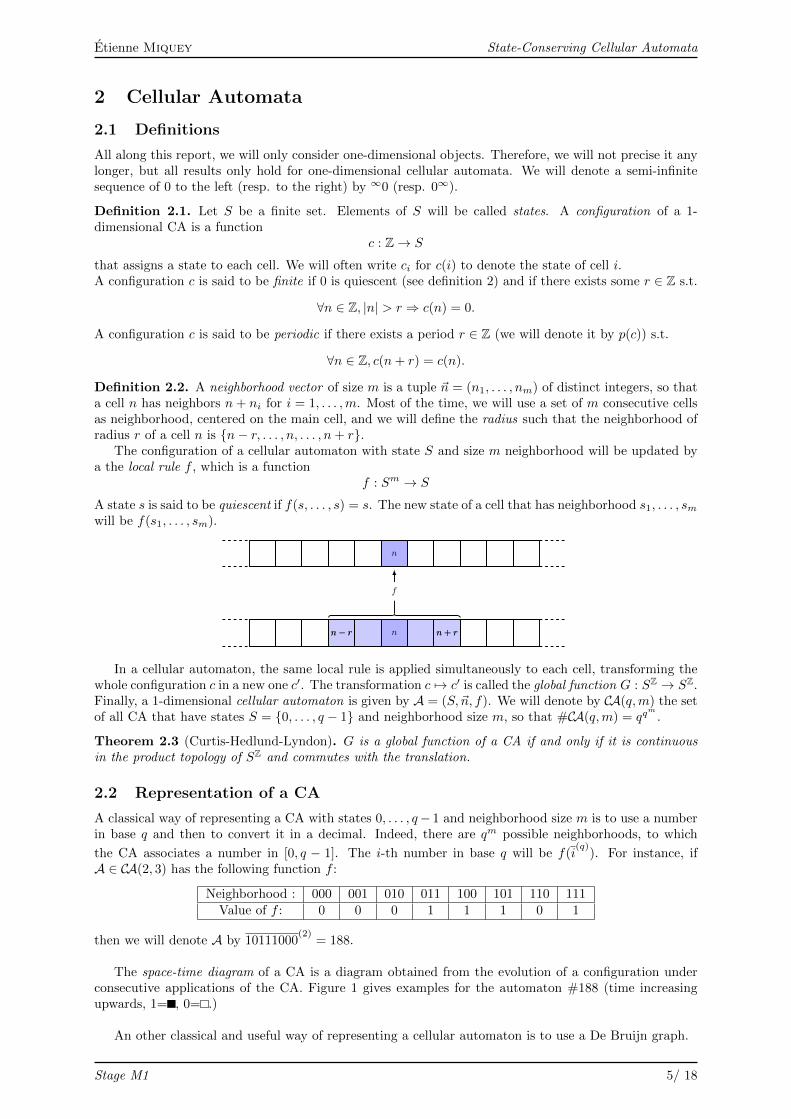
n− r n n+ rn− r

n

n+ r

f

In a cellular automaton, the same local rule is applied simultaneously to each cell, transforming thewhole configuration c in a new one c′. The transformation c 7→ c′ is called the global function G : SZ → SZ.Finally, a 1-dimensional cellular automaton is given by A = (S,~n, f). We will denote by CA(q,m) the setof all CA that have states S = {0, . . . , q − 1} and neighborhood size m, so that #CA(q,m) = qq

m

.

Theorem 2.3 (Curtis-Hedlund-Lyndon). G is a global function of a CA if and only if it is continuousin the product topology of SZ and commutes with the translation.

2.2 Representation of a CA

A classical way of representing a CA with states 0, . . . , q− 1 and neighborhood size m is to use a numberin base q and then to convert it in a decimal. Indeed, there are qm possible neighborhoods, to which

the CA associates a number in [0, q − 1]. The i-th number in base q will be f(i(q)

). For instance, ifA ∈ CA(2, 3) has the following function f :

Neighborhood : 000 001 010 011 100 101 110 111Value of f : 0 0 0 1 1 1 0 1

then we will denote A by 10111000(2)

= 188.

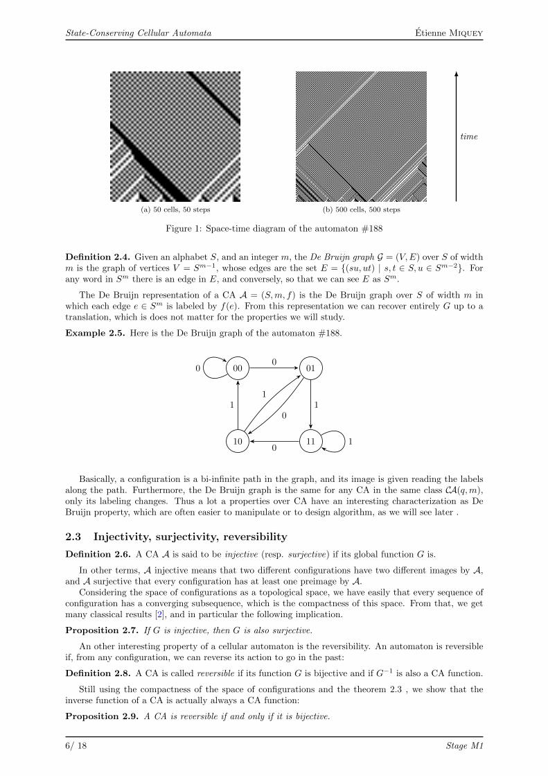
The space-time diagram of a CA is a diagram obtained from the evolution of a configuration underconsecutive applications of the CA. Figure 1 gives examples for the automaton #188 (time increasingupwards, 1= , 0= .)

An other classical and useful way of representing a cellular automaton is to use a De Bruijn graph.

Stage M1 5/ 18


(a) 50 cells, 50 steps (b) 500 cells, 500 steps

time

Figure 1: Space-time diagram of the automaton #188

Definition 2.4. Given an alphabet S, and an integer m, the De Bruijn graph G = (V,E) over S of widthm is the graph of vertices V = Sm−1, whose edges are the set E = {(su, ut) | s, t ∈ S, u ∈ Sm−2}. Forany word in Sm there is an edge in E, and conversely, so that we can see E as Sm.

The De Bruijn representation of a CA A = (S,m, f) is the De Bruijn graph over S of width m inwhich each edge e ∈ Sm is labeled by f(e). From this representation we can recover entirely G up to atranslation, which is does not matter for the properties we will study.

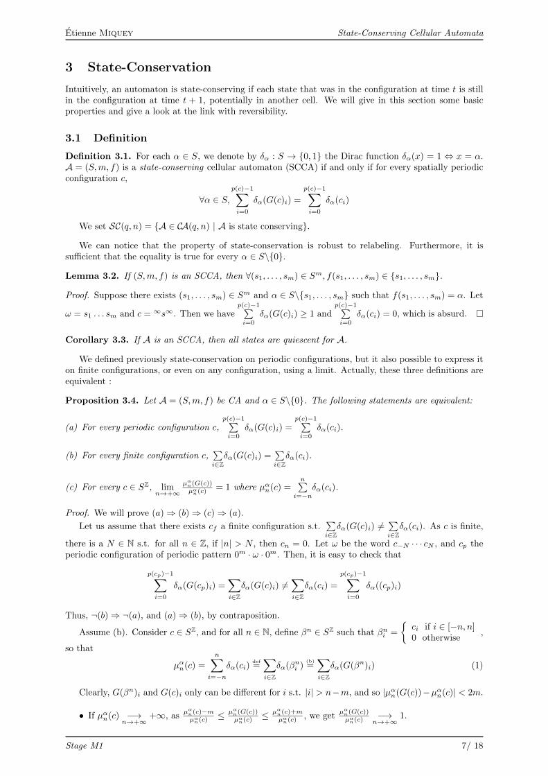
Example 2.5. Here is the De Bruijn graph of the automaton #188.

00 01

10 11

00

01

11

10

Basically, a configuration is a bi-infinite path in the graph, and its image is given reading the labelsalong the path. Furthermore, the De Bruijn graph is the same for any CA in the same class CA(q,m),only its labeling changes. Thus a lot a properties over CA have an interesting characterization as DeBruijn property, which are often easier to manipulate or to design algorithm, as we will see later .

2.3 Injectivity, surjectivity, reversibility

Definition 2.6. A CA A is said to be injective (resp. surjective) if its global function G is.

In other terms, A injective means that two different configurations have two different images by A,and A surjective that every configuration has at least one preimage by A.

Considering the space of configurations as a topological space, we have easily that every sequence ofconfiguration has a converging subsequence, which is the compactness of this space. From that, we getmany classical results [2], and in particular the following implication.

Proposition 2.7. If G is injective, then G is also surjective.

An other interesting property of a cellular automaton is the reversibility. An automaton is reversibleif, from any configuration, we can reverse its action to go in the past:

Definition 2.8. A CA is called reversible if its function G is bijective and if G−1 is also a CA function.

Still using the compactness of the space of configurations and the theorem 2.3 , we show that theinverse function of a CA is actually always a CA function:

Proposition 2.9. A CA is reversible if and only if it is bijective.

6/ 18 Stage M1


3 State-Conservation

Intuitively, an automaton is state-conserving if each state that was in the configuration at time t is stillin the configuration at time t + 1, potentially in another cell. We will give in this section some basicproperties and give a look at the link with reversibility.

3.1 Definition

Definition 3.1. For each α ∈ S, we denote by δα : S → {0, 1} the Dirac function δα(x) = 1 ⇔ x = α.A = (S,m, f) is a state-conserving cellular automaton (SCCA) if and only if for every spatially periodicconfiguration c,

∀α ∈ S,p(c)−1∑i=0

δα(G(c)i) =

p(c)−1∑i=0

δα(ci)

We set SC(q, n) = {A ∈ CA(q, n) | A is state conserving}.

We can notice that the property of state-conservation is robust to relabeling. Furthermore, it issufficient that the equality is true for every α ∈ S\{0}.

Lemma 3.2. If (S,m, f) is an SCCA, then ∀(s1, . . . , sm) ∈ Sm, f(s1, . . . , sm) ∈ {s1, . . . , sm}.

Proof. Suppose there exists (s1, . . . , sm) ∈ Sm and α ∈ S\{s1, . . . , sm} such that f(s1, . . . , sm) = α. Let

ω = s1 . . . sm and c = ∞s∞. Then we havep(c)−1∑i=0

δα(G(c)i) ≥ 1 andp(c)−1∑i=0

δα(ci) = 0, which is absurd.

Corollary 3.3. If A is an SCCA, then all states are quiescent for A.

We defined previously state-conservation on periodic configurations, but it also possible to express iton finite configurations, or even on any configuration, using a limit. Actually, these three definitions areequivalent :

Proposition 3.4. Let A = (S,m, f) be CA and α ∈ S\{0}. The following statements are equivalent:

(a) For every periodic configuration c,p(c)−1∑i=0

δα(G(c)i) =p(c)−1∑i=0

δα(ci).

(b) For every finite configuration c,∑i∈Zδα(G(c)i) =

∑i∈Zδα(ci).

(c) For every c ∈ SZ, limn→+∞

µαn(G(c))µαn(c) = 1 where µαn(c) =

n∑i=−n

δα(ci).

Proof. We will prove (a)⇒ (b)⇒ (c)⇒ (a).

Let us assume that there exists cf a finite configuration s.t.∑i∈Zδα(G(c)i) 6=

∑i∈Zδα(ci). As c is finite,

there is a N ∈ N s.t. for all n ∈ Z, if |n| > N , then cn = 0. Let ω be the word c−N · · · cN , and cp theperiodic configuration of periodic pattern 0m · ω · 0m. Then, it is easy to check that

p(cp)−1∑i=0

δα(G(cp)i) =∑i∈Z

δα(G(c)i) 6=∑i∈Z

δα(ci) =

p(cp)−1∑i=0

δα((cp)i)

Thus, ¬(b)⇒ ¬(a), and (a)⇒ (b), by contraposition.

Assume (b). Consider c ∈ SZ, and for all n ∈ N, define βn ∈ SZ such that βni =

{ci if i ∈ [−n, n]0 otherwise

,

so that

µαn(c) =

n∑i=−n

δα(ci)def=∑i∈Z

δα(βni )(b)=∑i∈Z

δα(G(βn)i) (1)

Clearly, G(βn)i and G(c)i only can be different for i s.t. |i| > n−m, and so |µαn(G(c))−µαn(c)| < 2m.

� If µαn(c) −→n→+∞

+∞, asµαn(c)−mµαn(c) ≤ µαn(G(c))

µαn(c) ≤ µαn(c)+mµαn(c) , we get

µαn(G(c))µαn(c) −→

n→+∞1.

Stage M1 7/ 18


� Otherwise, there exists N0 ∈ N such that ∀n ≥ N0, δα(c−n) = δα(cn) = 0. In particular, for alli s.t. N0 + m ≤ |i| ≤ N0 + 2m = N , ci 6= α. Using the Lemma 3.2, we get that for all i s.t.N −m ≤ |i| ≤ N, δα(G(c)i) = δα(G(βN )i) = 0, and as ∀i > N, δα(G(c)i) = 0, for all n > N :

µαn(G(c)) =∑i∈Z

δα(G(c)i) =

N∑i=−N

δα(G(c)i) =

N∑i=−N

δα(G(βN )i)(a)= µαN (c) = µαn(c)

Henceµαn(f(c))µαn(c) −→

n→+∞1.

Let us assume (c). Let c be a spatially periodic configuration. From the periodicity, we get that there

exists A,B ∈ N s.t. ∀k ∈ Z,p(c)−1∑i=0

δα(f(c)k+i) = A andp(c)−1∑i=0

δα(ck+i) = B. Thus, for all n ∈ N, we have

µαnp(c)(f(c)) = 2nA + f(c)0 and µαnp(c)(c) = 2nB + c0. So thatµαnp(c)(f(c))

µαnp(c)

(c) → AB Applying (c), we get

AB = 1, which implies (a).

3.2 Reversibility

A usual question in the study of a subclass of cellular automata is to know its relation with the reversibility.We will show here that reversible SCCA have state-conserving reverse automata, and that the subclassesof state-conserving CA and reversible CA have a non-empty intersection and are not included one in theother.

Proposition 3.5. Let A be an SCCA. If A reversible, then A−1 is also state-conserving.

Proof. This is trivial using the characterization (c) of Proposition 3.4. Let c ∈ SZ, c′ = G−1(c), so thatc = G(c′). Easily, we have

limn→+∞

µαn(G−1(c))

µαn(c)= limn→+∞

µαn(c′)

µαn(G(c′))= 1.

In dimension 1, the reversibility of a cellular automaton is decidable. From propositions 2.7 and 2.9,we have that an automaton is reversible if and only if it is injective, what could be classicaly characterizedin terms of De Bruijn graphs.

Proposition 3.6. A is injective if and only if in its De Bruijn representation, two different bi-infinitepaths always have different labelings.

We build the pair graph (Vp, Ep) of the De Bruijn graph (V,E), made of vertices (a, b) ∈ V × V , inwhich there is an edge (a, b)→ (a′, b′) each time (a, a′) and (b, b′) are in E and have the same label. Onecan easily verify that there exists two two-way infinite paths in the De Bruijn if and only if the pair graphhas a cycle going through a vertex out of the diagonal {(a, a) | a ∈ V }. This existence can for instancebe checked with an adapted depth-first search algorithm.

It appears that there exists both reversible and non-reversible non-trivial SCCA. Thereafter are ex-amples of one of each.

Example 3.7. The automaton #188 is an SCCA, but is not reversible. Indeed, both configurations∞01010∞ and ∞01100∞ will have ∞01010∞ for image. Actually, this automaton is not even surjective,since the very same configuration ∞0110∞ does not have any preimage by G.

G G

8/ 18 Stage M1


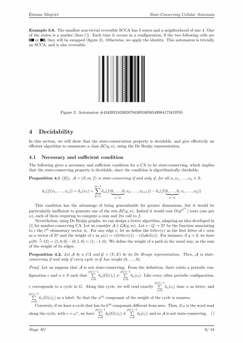
Example 3.8. The smallest non-trivial reversible SCCA has 3 states and a neighborhood of size 4. Oneof the states is a marker (here ). Each time it occurs in a configuration, if the two following cells are

or , they will be swapped (figure 2). Otherwise, we apply the identity. This automaton is triviallyan SCCA, and is also reversible.

Figure 2: Automaton #434392183362879438910056549984175819785

4 Decidability

In this section, we will show that the state-conservation property is decidable, and give effectivily anefficient algorithm to enumerate a class SC(q, n), using the De Bruijn representation.

4.1 Necessary and sufficient condition

The following gives a necessary and sufficient condition for a CA to be state-conserving, which impliesthat the state-conserving property is decidable, since the condition is algorithmically checkable.

Proposition 4.1 ([6]). A = (S,m, f) is state-conserving if and only if, for all α, x1, . . . , xn ∈ S,

δα(f(x1, . . . , xn)) = δα(x1) +

m−1∑k=1

δα(f(0, . . . , 0︸︷︷︸n−k

, x2, . . . , xk+1))− δα(f(0, . . . , 0︸︷︷︸n−k

, x1, . . . , xk))

This condition has the advantage of being generalisable for greater dimensions, but it would be

particularily inefficient to generate one of the sets SC(q, n). Indeed it would cost O(qqqm

) tests (one perα), each of them requiring to compute a sum and 2m call to f .

Nevertheless, using De Bruijn graphs, we can design a better algorithm, adapting an idea developed in[1] for number-conserving CA. Let us consider A ∈ CA(q,m). Let v : Q→ Zq be the function associatingto i the ith elementary vector ~ui. For any edge e, let us define the letter(e) as the first letter of e seenas a vector of Zq and the weight of e as µ(e) = v(letter(e))− v(label(e)). For instance, if q = 3, we have

µ(011→ 12) = (1, 0, 0)− (0, 1, 0) = (1,−1, 0). We define the weight of a path in the usual way, as the sum

of the weight of its edges.

Proposition 4.2. Let A be a CA and G = (V,E) be its De Bruijn representation. Then, A is state-conserving if and only if every cycle in G has weight (0, . . . , 0).

Proof. Let us suppose that A is not state-conserving. From the definition, there exists a periodic con-

figuration c and α ∈ S such thatp(c)−1∑i=0

δα(G(c)i) 6=p(c)−1∑i=0

δα(ci). Like every other periodic configuration,

c corresponds to a cycle in G. Along this cycle, we will read exactlyp(c)−1∑i=0

δα(ci) time α as letter, and

p(c)−1∑i=0

δα(G(c)i) as a label. So that the αth composant of the weight of the cycle is nonzero.

Conversly, if we have a cycle that has its kth composant different from zero. Then, if ω is the word read

along the cycle, with c = ω∗, we havep(c)−1∑i=0

δk(G(c)i) 6=p(c)−1∑i=0

δk(ci), and so A is not state-conserving.

Stage M1 9/ 18


4.2 Generating state-conserving rules

If G = (V,E, µ) is a weighted graph, we said that it admits ν : V → Zq as a potential function if and onlyif

∀(s, t) ∈ E, ν(t) = ν(s) + µ((s, t)). (2)

One can easily check that the following holds :

Proposition 4.3. A strongly connected weighted graph admits a potential function if and only if all itscycles have weight 0.

To list SC(q,m), we will enumerate CA(q,m) by labelling the edges, and backtrack as soon as a la-belling is not suitable for the existence of a potential function. The efficiency of the algorithm dependsof the way we go through the graph to label it. Indeed, each time we reach a vertex which already has apotential value, it constrains us for the label value, and avoid a lot of possibilities. We begin by sortingedges so as to encounter the maximum of constrains as soon as possible, by doing a depth-first search inwhich, at each step, we check first if any of the neighbors has already been reached. It gives us a sortedlist [e0, . . . , en−1] of edges. Then we call the algorithm 1 on SCCA(0).

Algorithm 1 SCCA(i)

Require: A list [e0, . . . , en−1] of the edges1: if i=n :2: add the current rule to the list, and return3: else4: /* ei ≡ si → ti */5: if ν(ei) is already defined :6: if it is possible to define label(ei) such that ν(ti) = ν(si) + µ(ei) :7: SCCA(i+ 1)8: end if9: else

10: for each α ∈ S :11: label(ei):=α12: ν(ti) := ~uα + ν(si)13: SCCA(i+1)14: end for15: erase the definition of ν(ti) and return16: end if17: end if

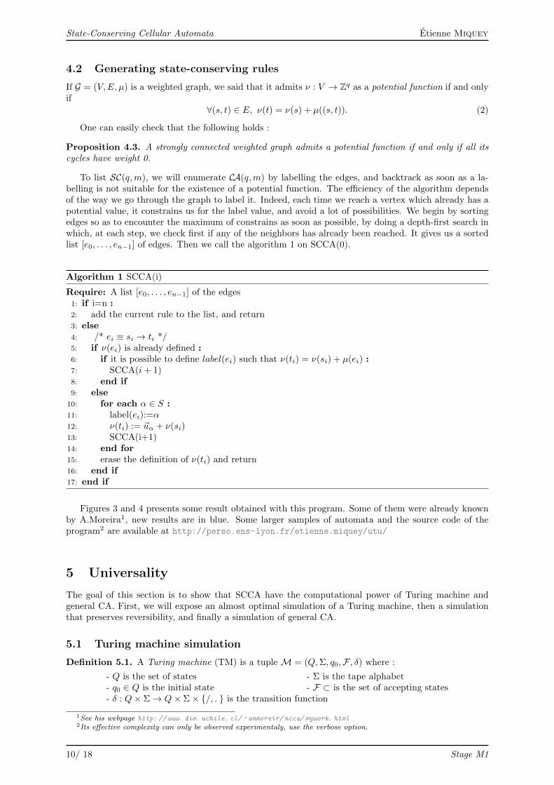
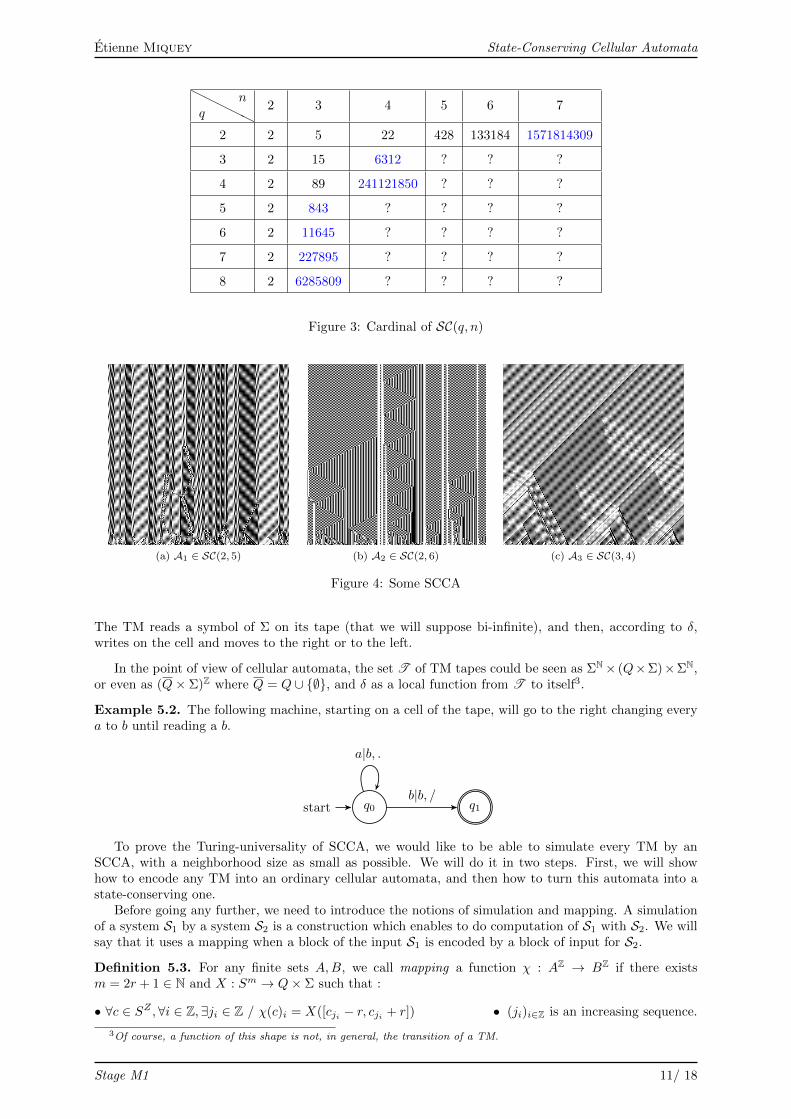
Figures 3 and 4 presents some result obtained with this program. Some of them were already knownby A.Moreira1, new results are in blue. Some larger samples of automata and the source code of theprogram2 are available at http://perso.ens-lyon.fr/etienne.miquey/utu/

5 Universality

The goal of this section is to show that SCCA have the computational power of Turing machine andgeneral CA. First, we will expose an almost optimal simulation of a Turing machine, then a simulationthat preserves reversibility, and finally a simulation of general CA.

5.1 Turing machine simulation

Definition 5.1. A Turing machine (TM) is a tuple M = (Q,Σ, q0,F , δ) where :

- Q is the set of states - Σ is the tape alphabet- q0 ∈ Q is the initial state - F ⊂ is the set of accepting states- δ : Q× Σ→ Q× Σ× {/, .} is the transition function

1See his webpage http: // www. dim. uchile. cl/ ~ anmoreir/ ncca/ mywork. html2Its effective complexity can only be observed experimentaly, use the verbose option.

10/ 18 Stage M1

http://perso.ens-lyon.fr/etienne.miquey/utu/

http://www.dim.uchile.cl/~anmoreir/ncca/mywork.html


HHHHHq

n2 3 4 5 6 7

2 2 5 22 428 133184 1571814309

3 2 15 6312 ? ? ?

4 2 89 241121850 ? ? ?

5 2 843 ? ? ? ?

6 2 11645 ? ? ? ?

7 2 227895 ? ? ? ?

8 2 6285809 ? ? ? ?

Figure 3: Cardinal of SC(q, n)

(a) A1 ∈ SC(2, 5) (b) A2 ∈ SC(2, 6) (c) A3 ∈ SC(3, 4)

Figure 4: Some SCCA

The TM reads a symbol of Σ on its tape (that we will suppose bi-infinite), and then, according to δ,writes on the cell and moves to the right or to the left.

In the point of view of cellular automata, the set T of TM tapes could be seen as ΣN× (Q×Σ)×ΣN,or even as (Q× Σ)Z where Q = Q ∪ {∅}, and δ as a local function from T to itself3.

Example 5.2. The following machine, starting on a cell of the tape, will go to the right changing everya to b until reading a b.

q0start q1

a|b, .

b|b, /

To prove the Turing-universality of SCCA, we would like to be able to simulate every TM by anSCCA, with a neighborhood size as small as possible. We will do it in two steps. First, we will showhow to encode any TM into an ordinary cellular automata, and then how to turn this automata into astate-conserving one.

Before going any further, we need to introduce the notions of simulation and mapping. A simulationof a system S1 by a system S2 is a construction which enables to do computation of S1 with S2. We willsay that it uses a mapping when a block of the input S1 is encoded by a block of input for S2.

Definition 5.3. For any finite sets A,B, we call mapping a function χ : AZ → BZ if there existsm = 2r + 1 ∈ N and X : Sm → Q× Σ such that :

• ∀c ∈ SZ ,∀i ∈ Z,∃ji ∈ Z / χ(c)i = X([cji − r, cji + r]) • (ji)i∈Z is an increasing sequence.

3Of course, a function of this shape is not, in general, the transition of a TM.

Stage M1 11/ 18


We denote by π the function i 7→ ji.

Definition 5.4. We will call simulation any couple (Φ, εφ) such that

1. for every TM M, Φ(M) = AM is a CA

2. εφ is a function from T to SZ, such that there exists χ verifying χ ◦ εφ = id

3. if we denote byM−→ (resp.

A−→) a step in M (resp. A), for any tape t ∈ T , the following diagramcommutes:

t M(t)

c G(c)

M

A

εφ εφ

We say that a simulation is minimal if, given the lengths |Q|, |Σ| there is no other simulation using asmaller radius. We say that a simulation uses a mapping if χ is a mapping.

If we have a simulation at our disposal, then it means that we are able to compute with A what Mwould do :

tεφ−→ c

A−→ G(c)χ−→M(t)

We shall note that εφ is necessarily injective, and χ surjective. Moreover, given the sets Q and Σ, theyare a finite number of Turing machines, and thus for every M, the radius of Φ(M) only depends on thelengths |Q| and |Σ|.

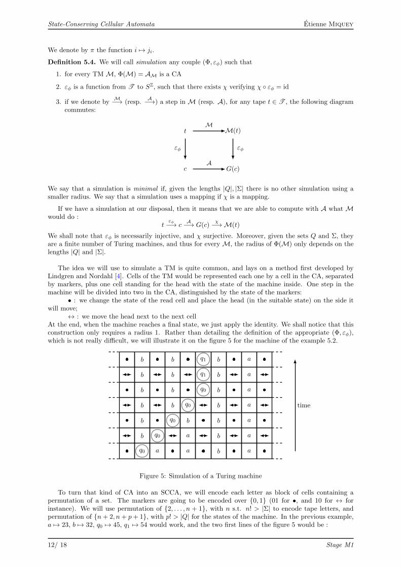
The idea we will use to simulate a TM is quite common, and lays on a method first developed byLindgren and Nordahl [4]. Cells of the TM would be represented each one by a cell in the CA, separatedby markers, plus one cell standing for the head with the state of the machine inside. One step in themachine will be divided into two in the CA, distinguished by the state of the markers:

• : we change the state of the read cell and place the head (in the suitable state) on the side itwill move;

↔ : we move the head next to the next cellAt the end, when the machine reaches a final state, we just apply the identity. We shall notice that thisconstruction only requires a radius 1. Rather than detailing the definition of the appropriate (Φ, εφ),which is not really difficult, we will illustrate it on the figure 5 for the machine of the example 5.2.

time

q0 a

b q0

b

b

b

b

b

a

a

q0 b

b q0

b

b

b

b

b

b

b

bq0

bq1

bq1

a

a

a

a

a

a

a

Figure 5: Simulation of a Turing machine

To turn that kind of CA into an SCCA, we will encode each letter as block of cells containing apermutation of a set. The markers are going to be encoded over {0, 1} (01 for •, and 10 for ↔ forinstance). We will use permutation of {2, . . . , n + 1}, with n s.t. n! > |Σ| to encode tape letters, andpermutation of {n+ 2, n+ p+ 1}, with p! > |Q| for the states of the machine. In the previous example,a 7→ 23, b 7→ 32, q0 7→ 45, q1 7→ 54 would work, and the two first lines of the figure 5 would be :

12/ 18 Stage M1


0 1 4 5 2 3 0 1 2 3 0 1 3 2 0 1 2 3 0 1

1 0 3 2 4 5 1 0 2 3 1 0 3 2 1 0 2 3 1 0time

To ensure that the automaton is state-conserving, we apply the identity on every block of cells whichdoes not correspond to a valid encoding, for instance if there are two heads of a TM side by side, or ifthe block is not between two markers of the same kind. Therefore, it requires to have a radius r suchthat r ≥ n + p + 1, for the last cell of the head to see the whole block on its side until the head of themarker, and S has to be {0, . . . , n + p + 1}. As it is locally state-conserving on any block between twomarkers, one can easily check that the automaton is an SCCA.

We could also have used permutations to encode directly couples of (Q×Σ)⋃

(Σ×Q), in which casen would have had to be greater than 2|Q||Σ|, and radius to be r = n+ 1 to see the whole block. This isin general slightly better as soon as |Q| and |Σ| grow.

Theorem 5.5. IfM = (Q,Σ, q0,F , δ) is a Turing machine, n is such that n! > 2|Q||Σ|, then there existsA ∈ SC(n+ 2, 2n+ 1) that simulates M.

Then we have a construction with a radius sub-logarithmic in the alphabets length. The next propo-sition show that this is not possible to have a constant radius, and that in fact, the simulation we exposedhas the best order of magnitude.

Proposition 5.6. Assume that we have a simulation (Φ, εφ) using a mapping and such that for everyTuring machine M, φ(M) is an SCCA. Let Q and Σ be some fixed alphabets, and r be the commonradius of all φ(Q,Σ, q0,F , δ). Then we have that (2r + 1)! = O(|Q||Σ|). Furthermore, if Φ is minimalthen the mapping verifies |π(1)− π(0)| ≥ 2r + 1.

Sketch of the proof. Let us denote Σ by {γ, α1, . . . , α|Σ|−1} and Q by {q0, . . . , q|Q|−1}. Consider a TMthat, in any state qj , will :

- move left each time it reads γ- change αi to αi+1 if i < |Σ| − 1 and move right- change α|Σ|−1 to α1, and qj to qj+1 (or stop if j = |Q| − 1).Let this machine start with the cell 0 containing α1, and 1 containing γ. Then, for every qj , the

TM heads will be |Σ| − 1 times on cell 0, each time reading a different letter. So that except the cell 0,everything on the tape is in the same state . As the diagram of the Definition 5.4 commutes, this is alsothe case in the image of the tape i.e. all the changes in the CA have to take place in the windows of 0:[π(0)− r, π(0) + r]. Which means that |Q|(|Σ| − 1) couples (q, α) can be encoded in that window, usingthe same CA states s1, . . . , sm (otherwise, it would not be state-conserving). Easily, we have that thebiggest number of possibilities of encoding with states s1, . . . , sm over m cells is to have ∀i 6= j, si 6= sj ,and that number is (m!). Hence m! > |Q|(|Σ| − 1).

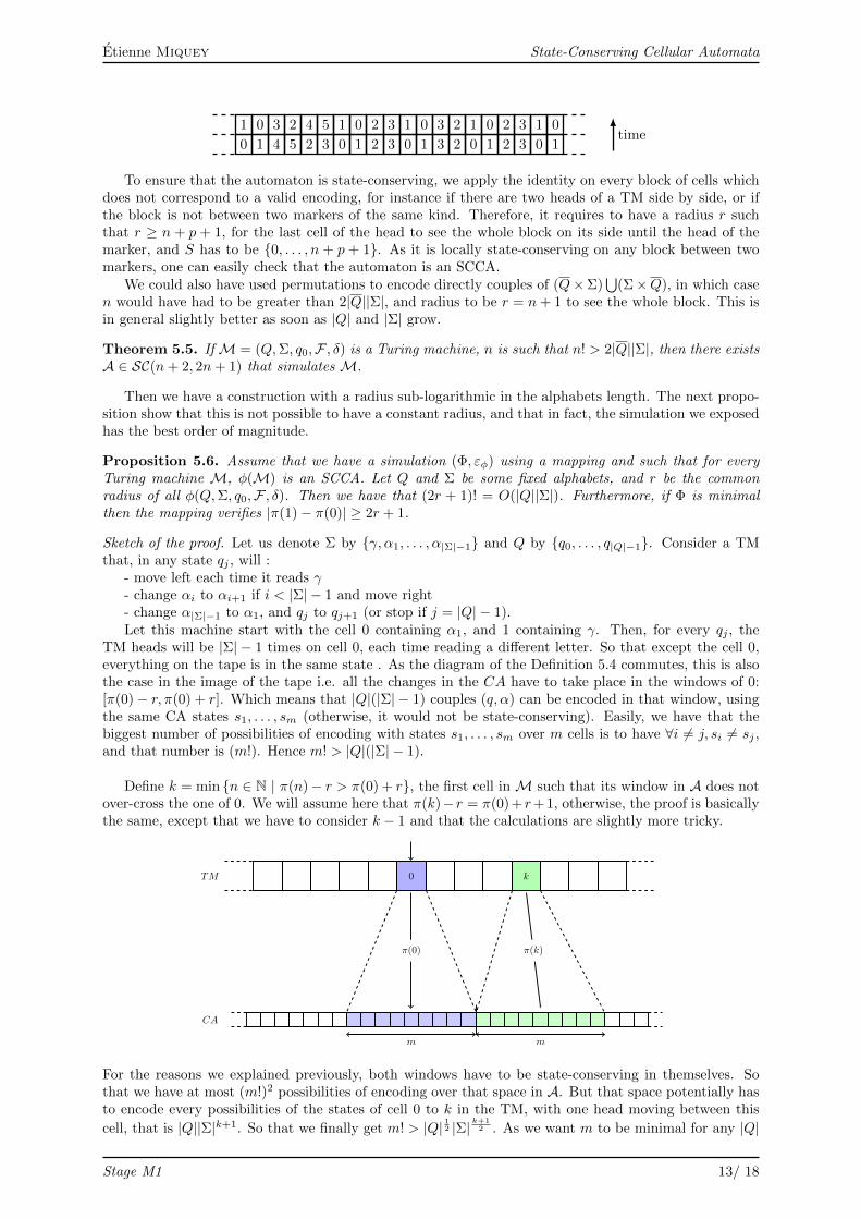
Define k = min {n ∈ N | π(n)− r > π(0) + r}, the first cell in M such that its window in A does notover-cross the one of 0. We will assume here that π(k)− r = π(0)+ r+1, otherwise, the proof is basicallythe same, except that we have to consider k − 1 and that the calculations are slightly more tricky.

0 kTM

CA

π(0) π(k)

m m

For the reasons we explained previously, both windows have to be state-conserving in themselves. Sothat we have at most (m!)2 possibilities of encoding over that space in A. But that space potentially hasto encode every possibilities of the states of cell 0 to k in the TM, with one head moving between this

cell, that is |Q||Σ|k+1. So that we finally get m! > |Q| 12 |Σ| k+12 . As we want m to be minimal for any |Q|

Stage M1 13/ 18


and |Σ|, it has to be better than the one we gave for the Proposition 5.6, so that in general we necessarilyhave:

|Q| 12 |Σ|k+12 ≤ 2|Q||Σ| ⇐⇒ |Σ|

k−12 ≤ 2|Q| 12

Therefore k = 1, which means that there is not any information over-crossing in the TM, as in theconstruction we presented above.

Thus our construction has an optimal order of magnitude, under the hypothesis that the simulationuses a mapping. Getting a smaller would require another concept of simulation. Nevertheless, this is nottotally satisfying, because it does not preserve the reversibility. Indeed, if M is a reversible TM, andAM the automaton we obtain, AM is reversible on valid configurations (that is {εφ(t) | t ∈ T }), but ingeneral is not reversible on any configuration.

5.2 Reversible simulation

We will here describe an other method of simulation preserving the reversibility on any configuration.This construction is inspired from work of Morita [7], using first a partitioned cellular automaton.

Definition 5.7. A partitioned cellular automaton (PCA) is a CA of local function f such that r = 1 andthere exists L,C,R some finite sets such that :

• S = L× C ×R • f : R× C × L→ L× C ×R

The idea is that the neighborhood is made of the center part of a cell, the right part of the left cell,and the left part of the right cell, so that at a step, one part (left, center, right) of a cell is only used onceto compute the next configuration. Which leads to following lemma :

Lemma 5.8. [7] If A is a PCA, then A is globally reversible if and only if it is locally reversible.

In other terms, to have A reversible, it is sufficient to define f as a bijection, which is quite easy.Indeed, f is defined between two sets of same cardinal, so that we only have to define it bijectively onthe subset that interests us, and then to extend it.

Briefly, we recall here the construction given in [7] to simulate a TM. We use an other definition ofTMs, which is equivalent to the one we gave, in which head moves and tape writing are separated in twosteps, and F = {qf}. Formally, we add a new symbol O, and for all (q, a) ∈ Q×Σ, either δ(q, a) = q′, b,O,either δ(q, a) = q′, a, //..

In our PCA, we have L = R = Q ∪ {•, ?} and C = L × Σ. For a given machine M, f is defined asfollow :

a) f(•, (q, a), •) = (•, (q′, b), •) if δ(q, a) = q′, b,O b) f(•, (q, a), •) = (q′, (•, a), •) if δ(q, a) = q′, a, /c) ∀q ∈ Q, f(•, (•, a), q) = (•, (q, a), •) d) ∀q ∈ Q, f(q, (•, a), •) = (•, (q, a), •)e) f(•, (?, a), ?) = (•, (q0, a), •) f) f(•, (qf , a), •) = (•, (?, a), ?)g) f(?, (•, a), •) = (?, (•, a), ?) h) f(•, (?, a), •) = (•, (?, a), •)

Rules (a-b) describe the computation ofM, (c-d) manage the head moves, and (e-h) handle reversibil-ity after the machine halts and before it begins.

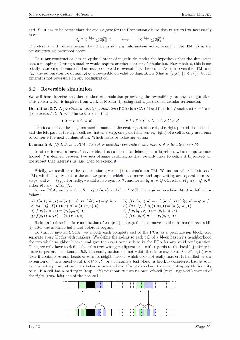
To turn it into an SCCA, we encode each complete cell of the PCA as a permutation block, andseparate every blocks with markers. We define the radius so each cell of a block has in its neighborhoodthe two whole neighbor blocks, and give the exact same rule as in the PCA for any valid configuration.Then, we only have to define the rules over wrong configurations, with regards to the local bijectivity inorder to preserve the Lemma 5.8. If a configuration c is not valid, that is to say for all t ∈ T , εφ(t) 6= c,then it contains several heads or ? in its neighborhood (which does not really matter, it handled by theextension of f to a bijection of L×C ×R), or c contains a bad block. A block is considered bad as soonas it is not a permutation block between two markers. If a block is bad, then we just apply the identityto it. If a cell has a bad right (resp. left) neighbor, it uses its own left-cell (resp. right-cell) instead ofthe right (resp. left) one of the bad cell :

14/ 18 Stage M1


Proposition 5.9. IfM is a reversible TM, then the corresponding automaton AM is a reversible SCCA.

Proof. There are two points to check. Firstly that AM is effectively state-conserving, but as a block iseither a permutation, either a wrong one preserved by the identity, this is obvious. Secondly that theautomaton is reversible. If the configuration is valid, this is the exact result given in [7]. If it is not, weonly have to see if there is any ambiguity around bad cells. But as each part of cell is still used onceand only once, the Lemma 5.8 still holds, and as the Turing rule is reversible, there is always exactly oneimage and one preimage.

It is easy to check that we have indeed defined a valid simulation, that is with a way of going from aTM tape to a CA configuration, and the way back. If we take a universal Turing machine as input of oursimulation, we will obviously have a CA Turing-universal. As a consequence, and due to the existence ofuniversal reversible Turing machines, we get the following theorem :

Theorem 5.10. There exists a reversible Turing-universal SCCA.

5.3 Intrinsically universal automaton

In this section, we will show how to simulate any CA by an SCCA in such a way that the simulationpreserves reversibility. Thanks to this, we will be able to derive many usual results for general CA. Wecan easily adapt the definition 5.4 to define the simulation of a CA by another CA.

Let us denote by A the automaton we want to simulate, and by ASC the one we will build. The ideais still the same, a cell is encoded by a block, and blocks are separated by markers. In that way, we havethe same complexity that we used to have for TM simulation, and actually we can slightly adapt theproof of the Proposition 5.6 to show that there is no really better way of doing it using a mapping.

As usual, the problem is to conserve reversibility when there are bad cells. For that, we will use adouble-layer automaton, in which each cell is a couple, standing for both layers. The upper layer is ruledby the same rule than A, and the lower one, by the symmetric one (left neighbors become the right ones,and conversely). On valid configuration, we only pay attention to the upper one, setting at the beginningthe second one to configuration 0∗ and letting the layer evolve. Obviously, in that case, if A is reversible,so is ASC . Now, when there is a bad cell, as usual we apply to it the identity, and the its neighbors usethe low layer. The right neighbor of a bad cell will use its usual right neighbors, but its left neighbor isnow its low part, the second left neighbor is the low part of its right neighbor, and so on:

Proposition 5.11. If a CA A is reversible, so is its corresponding SCCA ASC.

Proof. Let c be any configuration for ASC . Let us pick a valid connected component (that is without badcell). There are three cases:

1. The component is the whole configuration, obviously it has exactly one preimage by ASC .

2. The component is semi-infinite. Then, we can consider the two layers as one valid configurationwho would have been fold down.

3. The component is folded. Then, we can consider the two layers as a ring, and so the componentbehaves exactly as a valid periodic configuration.

Hence c has exactly one preimage by ASC .

Definition 5.12. An automaton is said to be intrinsically universal if it is able to simulate any otherCA.

As our construction clearly is a simulation in the sense of the Definition 5.4, it is obvious that if a CAis intrinsically universal, so is its simulation by an SCCA. Using the existence of an intrinsically universalCA [8], we get the same result for SCCA :

Theorem 5.13. There exists an intrinsically universal SCCA.

Stage M1 15/ 18


6 Undecidable problems

6.1 1-dimensional SCCA

One of the motivation of the previous constructions is to be easily able to reduce a lot of undecidabilityproblem to SCCA. An immediate corollary of our last simulation, that preserves intrinsically universality,is the undecidability of this property :

Theorem 6.1. The intrinsic universality problem is undecidable over SCCA.

Proof. This problem is undecidable for CA in general [8]. As our construction preserves intrinsic univer-sality, this is also true for SCCA.

We will give here two other examples of decision problem for reversible CA that are reducible toreversible SCCA, namely periodicity and immortality problems.

A CA is said to be periodic if ∀c ∈ SZ,∃n ∈ N s.t. Gn(c) = c. This problem is undecidable forreversible CA [3], and we can prove the same thing for SCCA. We should note previously that in cellularautomata periodicity and uniform periodicity are equivalent. Indeed, let A be a periodic CA and supposethat for all n ≥ 1, there exists cn ∈ SZ s.t. Gn(cn) 6= cn. Each cn has a finite segment pn which is mappedin n steps into a state which is different from the center of pn. If a configuration c contains every pn,then c is not periodic for A, which is absurd.

Theorem 6.2. It is undecidable whether a reversible SCCA is periodic.

Proof. Let A be a reversible CA, ASC the reversible automaton obtained with the simulation (Φ, εφ) ofsection 5.3. We have to show that ASC is periodic if and only if A is. If there exists a configuration cwhich is not periodic for A, clearly εφ(c) is not periodic for ASC . Conversely, if A is periodic, ASC is alsoperiodic on every valid configurations.

For the other ones, the reasoning is very similar to the proof we did for the Proposition5.11. Weconsider once more the connected components, each of them being periodic. Since periodicity impliesuniform periodicity, there exists in A a common period n to every connected component, and thus anyconfiguration is periodic.

Let H be a set of halting states. A configuration c is said halting if there exists i ∈ Z s.t. ci ∈ H. ACA is said to be mortal if for all c ∈ SZ, there exists n ∈ N s.t. Gn(c) is halting. It is also undecidablewhether a reversible CA is immortal[3]. Clearly, as states are conserved all along the execution, thisproblem is trivial for a SCCA. Nonetheless, if we change a little the problem to have H′ a finite set offinite patterns, and said that an automaton is pattern-mortal if there exists a segment [a, b] ⊂ Z s.t.c[a,b] ∈ H′, this problem turns to be undecidable:

Theorem 6.3. The pattern-mortality problem is undecidable for reversible SCCA.

Proof. Let A (of global function G) be a reversible CA, H be a set of states of A, and ASC the reversibleautomaton (of function GSC) obtained with the simulation (Φ, εφ) of section 5.3. For every pattern h ofH, we denote by h its corresponding pattern for ASC determined by εφ. If a cell is encoded over a blockof size b, we define B as the finite set of bad blocks of size b, which are those that could not be found intoa valid configuration. Finally we set H′ = {h | h ∈ H}∪B and claim that A is mortal if and only if ASCis pattern-mortal.

Indeed, ifA is immortal, there exists a configuration c such that for all i ∈ Z, for all n ∈ N, Gn(c)i /∈ H.Then for all i ∈ Z, for all n ∈ N, GnSC(εφ(c))[i,i+b] /∈ H′. Conversely, assume A is mortal. Let c be aconfiguration for ASC . Either it is a valid configuration, and then its preimage is mortal for A, and c ispattern-halting for ASC . Either it is not, and then there exists an i ∈ Z such that c[i,i+b] ∈ B. In bothcases, c is pattern-halting for ASC , which proves that ASC is pattern-mortal.

6.2 2-dimensional SCCA

We will not give here formal definitions, but most of the time, all the definitions we gave before canbe extended to d-dimensional CA, replacing everywhere Z by Zd. If we only focus on 2-dimensionalCA, adapting works that have been done for number-conserving cellular automata (the definition is thesame, without using δα), we can show that the proposition 3.4 still holds. In addition, we still have thedecidability of the state-conserving problem, with a result analogous to the proposition 4.1. Nevertheless,De Bruijn graph does not exist for 2-CA, we have no efficient algorithm a priori.

16/ 18 Stage M1


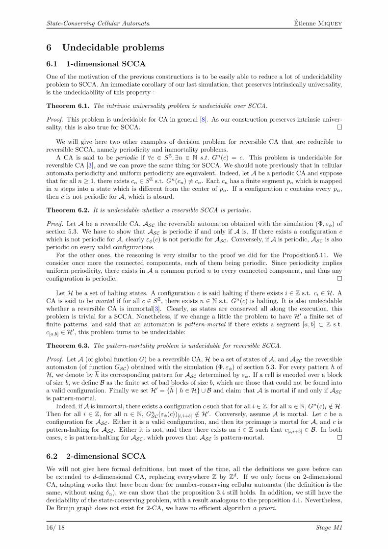
Clearly, we can simulate any 2-CA by a 2-SCCA, with the same kind of ideas we used previously.We encode each cell by a permutation block of a rectangular shape (to be able to tile the plane), andseparate blocks by a border of marker. For instance, to encode a 2-CA until 24 states, we will use asmarker, and as states. The encoding of a configuration will look like this :

We know that reversibility is undecidable for 2-CA, and we would like to reduced this problem for2-SCCA :

Conjecture 6.4. Reversibility is undecidable for 2-SCCA.

A simulation preserving the reversibility would be sufficient to prove that reversibility is still unde-cidable for 2-SCCA. We sketch here a construction similar to the one we exposed for 1-CA, but we donot know whether it is suitable (see Question 5).

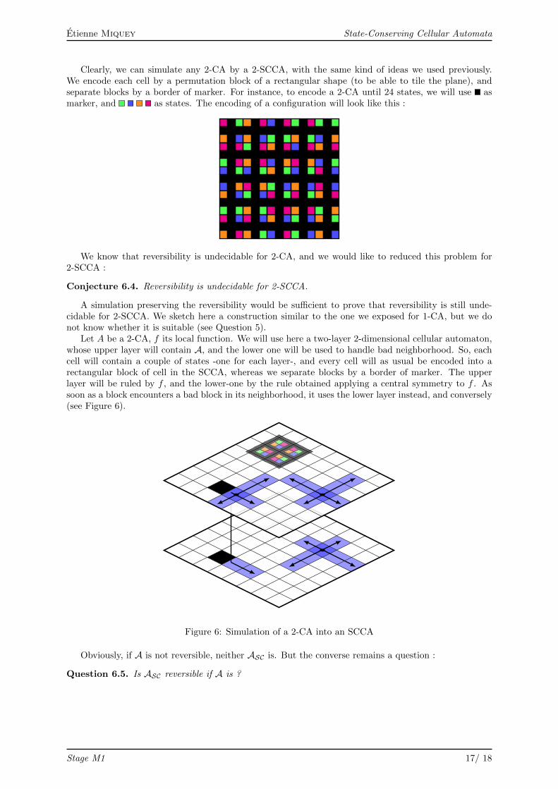
Let A be a 2-CA, f its local function. We will use here a two-layer 2-dimensional cellular automaton,whose upper layer will contain A, and the lower one will be used to handle bad neighborhood. So, eachcell will contain a couple of states -one for each layer-, and every cell will as usual be encoded into arectangular block of cell in the SCCA, whereas we separate blocks by a border of marker. The upperlayer will be ruled by f , and the lower-one by the rule obtained applying a central symmetry to f . Assoon as a block encounters a bad block in its neighborhood, it uses the lower layer instead, and conversely(see Figure 6).

Figure 6: Simulation of a 2-CA into an SCCA

Obviously, if A is not reversible, neither ASC is. But the converse remains a question :

Question 6.5. Is ASC reversible if A is ?

Stage M1 17/ 18


7 Conclusion

We made here a first study of state-conserving cellular automata, and deal with some of their basicproperties. Then we gave a characterization of state-conservation over De Bruijn graph, and implementedan efficient algorithm to list the classes SC(q, n). We also designed simulation preserving the reversibilityto enhanced the universality of state-conserving cellular automata, and illustrate their utility by somefew examples of reduction of decision problem. This might be a good first basis for any further work onthis class of automaton in the future. Moreover, in addition to the question 6.5, one can wonder if theautomaton A1 and A2 on Figure 4 are Turing universal, because they seem to behave like the rule 110(which was proved universal by Cook), with a propagation of signals.

For a more personal aspect, this internship has enabled me to discover the theory of cellular automatastarting from scratch. In that sense, it was particularly interesting, since it made me get familiar to CAthanks to some lectures note from a course Jarkko gives inT urku and some few papers. And it has aboveall given me basics knowledges in a new topic, with its related points of view and questions.

References

[1] Bastien Le Gloannec, Around kari’s traffic cellular automaton for the density classification task, 2009.

[2] Jarkko Kari, Theory of cellular automata: A survey, Theoretical Computer Science 334 (2005), no. 1-3, 3 – 33.

[3] Jarkko Kari and Nicolas Ollinger, Periodicity and Immortality in Reversible Computing, Additionalmaterial available on the web at http://www.lif.univ-mrs.fr/nollinge/rec/gnirut/.

[4] K Lindgren and M Nordahl, Universal computation in simple one dimensional cellular automata,Complex Systems (1990), no. 4.

[5] A. Moreira, Universality and Decidability of Number-Conserving Cellular Automata, ArXiv NonlinearSciences e-prints (2003).

[6] A. Moreira, N. Boccara, and E. Goles, On Conservative and Monotone One-dimensional CellularAutomata and Their Particle Representation, ArXiv Nonlinear Sciences e-prints (2003).

[7] Kenichi Morita, Computation-universality of one-dimensional one-way reversible cellular automata,Inf. Process. Lett. 42 (1992), 325–329.

[8] Nicolas Ollinger, The intrinsic universality problem of one-dimensional cellular automata, STACS2003 (Helmut Alt and Michel Habib, eds.), Lecture Notes in Computer Science, vol. 2607, SpringerBerlin / Heidelberg, 2003, pp. 632–641.

18/ 18 Stage M1

state-conserving cellular automata etienneemiquey/stage/utu.pdf · state-conserving cellular...

Documents