STAT602XHomework 5

2011-04-17

Keys

20. Figure 4.4 of HTF gives a 2-dimensional plot of the ”vowel training data” (available on the

book’s website at http://www-stat.stanford.edu/~tibs/ElemStatLearn/index.html or from

http://archive.ics.uci.edu/ml/datasets/Connectionist+Bench+%28Vowel+Recognition+-+

Deterding+Data%29 ). The ordered pairs of first 2 canonical variates are plotted to give a ”best”

reduced rank LDA picture of the data like that below (lacking the decision boundaries).

a) Use Section 10.1 of the course outline to reproduce Figure 4.4 of HTF (color-coded by group,

with group means clearly indicated). Keep in mind that you may need to multiply one or both of

your coordinates by −1 to get the exact picture.

Use the R function lda (MASS package) to obtain the group means and coefficients of linear dis-

criminants for the vowel training data. Save the lda object by a command such as LDA=lda(insert

formula, data=vowel).

(5 pts)

– 1 –

STAT602XHomework 5

2011-04-17

Keys

−4 −2 0 2 4

−6

−4

−2

02

4

Linear Discriminant Analysis

Coordinate 1 for Training Data

Coo

rdin

ate

2 fo

r T

rain

ing

Dat

a

R Codevowel <- read.table("vowel.train", header = TRUE, sep = ",", quote = "")da <- vowel[, -1]color <- c("#60FFFF", "#B52000", "#FF99FF", "#20B500", "#FFCA00",

"red", "green", "blue", "grey75", "#FFB2B2", "#928F52")

Y <- da[, 1]X <- da[, -1]K <- length(unique(Y))N <- length(Y)p <- ncol(X)mu.k <- do.call("rbind", lapply(1:K, function(k) colMeans(X[Y == k,])))mu.bar <- colMeans(mu.k)

mu.k.tmp <- matrix(rep(t(mu.k), N / K), nrow = ncol(mu.k))Sigma <- (t(X) - mu.k.tmp) %*% t(t(X) - mu.k.tmp) / (N - K)Sigma.eigen <- eigen(Sigma)Sigma.inv.sqrt <- Sigma.eigen$vectors %*% diag(1/sqrt(Sigma.eigen$values)) %*%

t(Sigma.eigen$vectors)X.star <- t(Sigma.inv.sqrt %*% (t(X) - mu.bar))mu.k.star <- t(Sigma.inv.sqrt %*% (t(mu.k) - mu.bar))

M <- mu.k.starM.svd <- eigen(t(M) %*% M / K)

X.new <- X.star %*% M.svd$vectorsmu.k.new <- mu.k.star %*% M.svd$vectors

plot(-X.new[, 1], X.new[, 2], col = color[Y], pch = Y + 1,main = "Linear Discriminant Analysis",

– 2 –

STAT602XHomework 5

2011-04-17

Keys

xlab = "Coordinate 1 for Training Data", ylab = "Coordinate 2 for Training Data")points(-mu.k.new[, 1], mu.k.new[, 2], col = color[Y], pch = 19, cex = 1.5)

b) Reproduce a version of Figure 1a) above. You will need to plot the first two canonical coordinates

as in a). Decision boundaries for this figure are determined by classifying to the nearest group mean.

Do the classification for a fine grid of points covering the entire area of the plot. If you wish, you

may plot the points of the grid, color coded according to their classification, instead of drawing in

the black lines.

(5 pts)

−4 −2 0 2 4

−6

−4

−2

02

4

Classified to nearest mean

Coordinate 1

Coo

rdin

ate

2

R Codelibrary(MASS)LDA <- lda(y ~ ., data = da)X.pred <- predict(LDA, newdata = X)mu.k.pred <- predict(LDA, newdata = as.data.frame(LDA$means))

X.new <- X.pred$xmu.k.new <- mu.k.pred$x

x.lim <- range(X.new[, 1])

– 3 –

STAT602XHomework 5

2011-04-17

Keys

y.lim <- range(X.new[, 2])

x.grid <- 100y.grid <- 100grid <- cbind(seq(x.lim[1], x.lim[2], length = x.grid),

rep(seq(y.lim[1], y.lim[2], length = y.grid), each = x.grid))get.class <- function(grid, mu){K <- nrow(mu)apply(grid, 1, function(x) which.min(dist(rbind(x, mu))[1:K]))

}grid.class <- get.class(grid, mu.k.new[, 1:2])

plot(X.new[, 1], X.new[, 2], col = color[Y], type = "n",main = "Classified to nearest mean",xlab = "Coordinate 1", ylab = "Coordinate 2")

points(grid[, 1], grid[, 2], col = color[grid.class], pch = 19, cex = 0.3)points(X.new[, 1], X.new[, 2], pch = Y + 1, cex = 0.8)points(mu.k.new[, 1], mu.k.new[, 2], pch = 19, cex = 1.5)

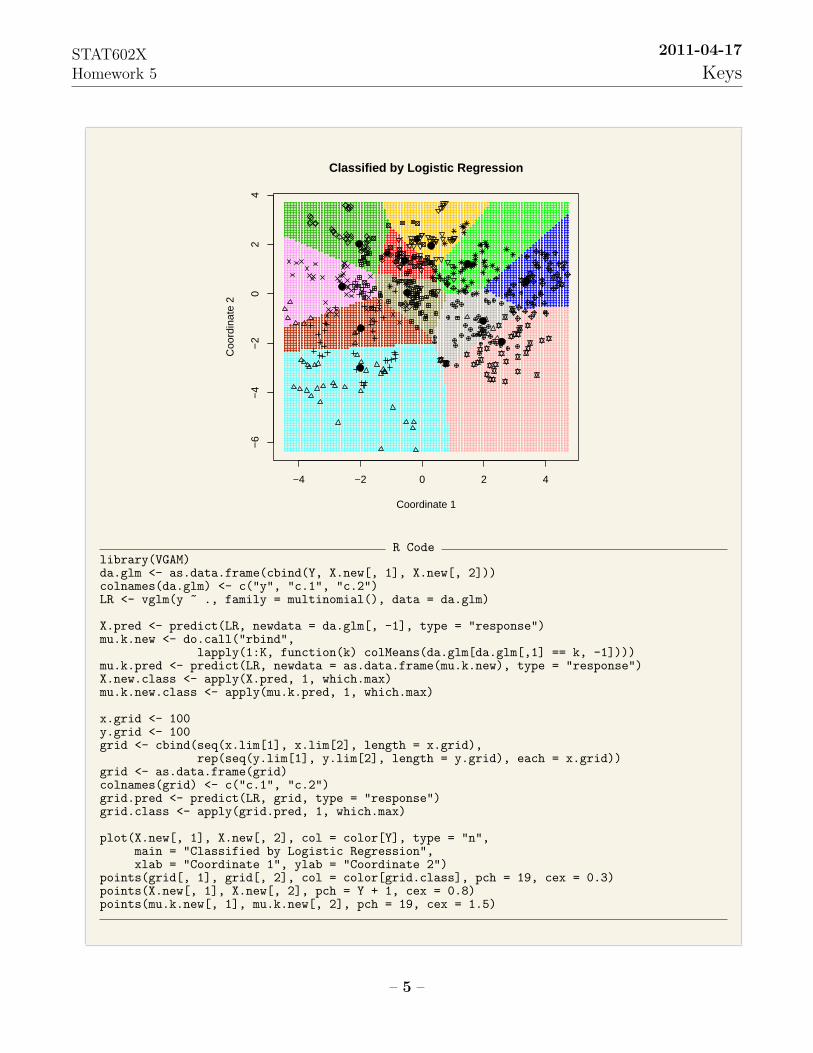
c) Make a version of Figure 1b) above with decision boundaries now determined by using logisitic

regression as applied to the first two canonical variates. You will need to create a data frame

with columns y, canonical variate 1, and canonical variate 2. Use the vglm function (VGAM

package) with family=multinomial() to do the logistic regression. Save the lda object by a

command such as LR=vglm(insert formula, family=multinomial(), data=data set). A set

of observations can now be classified to groups by using the command predict(LR, newdata,

type="response"), where newdata contains the observations to be classified. The outcome of

the predict function will be a matrix of probabilities. Each row contains the probabilities that a

corresponding observation belongs to each of the groups (and thus sums to 1). We classify to the

group with maximum probability. As in b), do the classification for a fine grid of points covering

the entire area of the plot. You may again plot the points of the grid, colorcoded according to their

classification, instead of drawing in the black lines.

(5 pts)

– 4 –

STAT602XHomework 5

2011-04-17

Keys

−4 −2 0 2 4

−6

−4

−2

02

4

Classified by Logistic Regression

Coordinate 1

Coo

rdin

ate

2

R Codelibrary(VGAM)da.glm <- as.data.frame(cbind(Y, X.new[, 1], X.new[, 2]))colnames(da.glm) <- c("y", "c.1", "c.2")LR <- vglm(y ~ ., family = multinomial(), data = da.glm)

X.pred <- predict(LR, newdata = da.glm[, -1], type = "response")mu.k.new <- do.call("rbind",

lapply(1:K, function(k) colMeans(da.glm[da.glm[,1] == k, -1])))mu.k.pred <- predict(LR, newdata = as.data.frame(mu.k.new), type = "response")X.new.class <- apply(X.pred, 1, which.max)mu.k.new.class <- apply(mu.k.pred, 1, which.max)

x.grid <- 100y.grid <- 100grid <- cbind(seq(x.lim[1], x.lim[2], length = x.grid),

rep(seq(y.lim[1], y.lim[2], length = y.grid), each = x.grid))grid <- as.data.frame(grid)colnames(grid) <- c("c.1", "c.2")grid.pred <- predict(LR, grid, type = "response")grid.class <- apply(grid.pred, 1, which.max)

plot(X.new[, 1], X.new[, 2], col = color[Y], type = "n",main = "Classified by Logistic Regression",xlab = "Coordinate 1", ylab = "Coordinate 2")

points(grid[, 1], grid[, 2], col = color[grid.class], pch = 19, cex = 0.3)points(X.new[, 1], X.new[, 2], pch = Y + 1, cex = 0.8)points(mu.k.new[, 1], mu.k.new[, 2], pch = 19, cex = 1.5)

– 5 –

STAT602XHomework 5

2011-04-17

Keys

21. Continue use of the vowel training data from problem 20.

a) So that you can see and plot results, first use the 2 canonical variates employed in problem 20

and use rpart in R to find a classification tree with empirical error rate comparable to the reduced

rank LDA classifier pictured in Figure 1a. Make a plot showing the partition of the region into

pieces associated with the 11 different classes.

(5 pts) I use default settings in lda() and rpart(), and the LDA result has the error about

0.3163 and regression partitioning has the error about 0.2576. The controls in rpart() use

a value of cp complexity parameter (default 0.1) to build a tree. Therefore, I prune the

tree according the value of cp in the prune() function to fit in a similar error of LDA. The

corresponding cp value is about 0.0167. The following plots show the tree result and final

classifications.

|X.1< 0.3979

X.2< −1.177

X.2< −2.744 X.1< −1.376

X.2< 1.68 X.2>=0.9215

X.2>=0.05988

X.1< 2.802

X.1< 1.123

X.2>=−2.173

1 2

3 4 6 11

5 7

8 9 10

−4 −2 0 2 4

−6

−4

−2

02

4

rpart on X.1 and X.2

Coordinate 1 for Training Data

Coo

rdin

ate

2 fo

r T

rain

ing

Dat

a

R Codevowel <- read.table("vowel.train", header = TRUE, sep = ",", quote = "")da <- vowel[, -1]Y <- da[, 1]X <- da[, -1]color <- c("#60FFFF", "#B52000", "#FF99FF", "#20B500", "#FFCA00",

"red", "green", "blue", "grey75", "#FFB2B2", "#928F52")

library(MASS)LDA <- lda(y ~ ., data = da)X.pred <- predict(LDA, newdata = X)X.1 <- X.pred$x[, 1]X.2 <- X.pred$x[, 2](error.LDA <- mean(as.numeric(X.pred$class) != Y))

library(rpart)

– 6 –

STAT602XHomework 5

2011-04-17

Keys

m.a <- rpart(as.factor(Y) ~ X.1 + X.2)pred.a <- predict(m.a, type = "class")(error.a <- mean(as.numeric(pred.a) != Y))

my.prune <- function(cp, m.r){mean(as.numeric(predict(prune(m.r, cp = cp), type = "class")) != Y) - error.LDA

}(ret.cp.a <- uniroot(my.prune, c(0.01, 0.02), m.a))m.cp.a <- prune(m.a, cp = ret.cp.a$root)pred.cp.a <- as.numeric(predict(m.cp.a, type = "class"))

par(mar = c(0, 0, 0, 0))plot(m.cp.a, compress = TRUE, margin = 0.1)text(m.cp.a)

plot(X.1, X.2, col = color[pred.cp.a], pch = pred.cp.a + 1, main = "rpart on X.1 and X.2",xlab = "Coordinate 1 for Training Data", ylab = "Coordinate 2 for Training Data")

b) Beginning with the original data set (rather than with the first 2 canonical variates) and use

rpart in R to find a classification tree with empirical error rate comparable to the classifier in a).

How much (if any) simpler/smaller is the tree here than in a)?

(5 pts) Again, the default settings in rpart() give me an error about 0.1629 based on original

data set. So, I prune the tree according the value of cp in the prune() function to fit in a

similar error of LDA. The corresponding cp value is about 0.0166. Comparing to the part a)

and the problem 20, this gives a better fit and more similar to the LDA results. Note that

the partition rules are more complex than that in the part a).

|X[, 2]< 0.639

X[, 2]< −0.1235

X[, 1]< −3.568

X[, 1]>=−3.143

X[, 1]>=−2.313

X[, 2]< 1.098X[, 2]>=2.04

X[, 1]>=−3.008

X[, 5]>=−1.019

X[, 1]>=−4.668

X[, 8]< 0.056

X[, 4]< −0.021X[, 1]>=−3.979

X[, 3]< −0.936

X[, 8]< 0.909

X[, 1]>=−3.562X[, 2]>=1.976

1

1 2

3 4

5 7 11

2

7 8 9

10 9

107 9

8

−4 −2 0 2 4

−6

−4

−2

02

4

rpart on original data

Coordinate 1 for Training Data

Coo

rdin

ate

2 fo

r T

rain

ing

Dat

a

– 7 –

STAT602XHomework 5

2011-04-17

Keys

R Codeformula <- as.formula(paste("as.factor(Y) ~ ", paste(paste("X[,", 1:10, "]", sep = ""),

collapse=" + "), sep = ""))m.b <- rpart(formula)pred.b <- predict(m.b, type = "class")(error.b <- mean(as.numeric(pred.b) != Y))

(ret.cp.b <- uniroot(my.prune, c(0.01, 0.02), m.b))m.cp.b <- prune(m.b, cp = ret.cp.b$root)pred.cp.b <- as.numeric(predict(m.cp.b, type = "class"))

par(mar = c(0, 0, 0, 0))plot(m.cp.b, compress = TRUE, margin = 0.1)text(m.cp.b)

plot(X.1, X.2, col = color[pred.cp.b], pch = pred.cp.b + 1, main = "rpart on original data",xlab = "Coordinate 1 for Training Data", ylab = "Coordinate 2 for Training Data")

22. Consider the famous Wisconsin Breast Cancer data set at http://archive.ics.uci.edu/ml/

datasets/Breast+Cancer+Wisconsin+%28Original%29 . Compare an appropriate SVM based on

the original input variables to a classifier based on logistic regression with the same variables.

(BTW, there is a nice paper ”Support Vector Machines in R” by Karatzoglou, Meyer, and Hornik

that appeared in Journal of Statistical Software that you can get to through ISU. And there is an

R SVM tutorial at http://planatscher.net/svmtut/svmtut.html .)

(10 pts) I take off patients with missing values ”?” and perform SVM and logistic regression

on the Breast Cancer data set. The results are shown in the following, and the error rates for

misclassification are (5 + 11)/682 ≈ 0.0235 for SVM and (10 + 11)/682 ≈ 0.0308 for logistic

regression.

R Output> da <- read.csv("breast-cancer-wisconsin.data", na.strings = "?")> colnames(da) <- c("Sample.code.number", "Clump.Thickness", "Uniformity.of.Cell.Size",+ "Uniformity.of.Cell.Shape", "Marginal.Adhesion", "Single.Epithelial.Cell.Size",+ "Bare.Nuclei", "Bland.Chromatin", "Normal.Nucleoli", "Mitoses", "Class")> da <- da[rowSums(is.na(da)) == 0,]> da.X <- as.matrix(da[, c(-1, -11)])> da.class <- as.factor(da[, 11])> library(e1071)> model.svm <- svm(da.X, da.class)> pred.svm <- predict(model.svm, da.X)> table(pred.svm, t(da.class))

pred.svm 2 42 432 54 11 234

> library(VGAM)> da.glm <- cbind(data.frame(y = da.class), da.X)> model.glm <- vglm(y ~ ., family = multinomial(), data = da.glm)

– 8 –

STAT602XHomework 5

2011-04-17

Keys

> pred.glm <- predict(model.glm, newdata = da.glm[, -1], type = "response")> pred.glm <- apply(pred.glm, 1, which.max)> pred.glm[pred.glm == 2] <- 4> pred.glm[pred.glm == 1] <- 2> table(pred.glm, t(da.class))

pred.glm 2 42 433 114 10 228

23. (Izenman Problem 14.4.) Consider the following 10 two-dimensional points, the first five

points, (1, 4), (3.5, 6.5), (4.5, 7.5), (6, 6), (1.5, 1.5), belong to Class 1 and the second five points

(8, 6.5), (3, 4.5), (4.5, 4), (8, 1.5), (2.5, 0), belong to Class 2. Plot these points on a scatterplot using

different symbols or colors to distinguish the two classes. Carry through by hand the AdaBoost

algorithm on these points, showing the weights at each step of the process. (Presumably Izenman’s

intention is that you use simple 2-node trees as your base classifiers.) Determine the final classifier

and calculate its empirical misclassification rate.

The results may depend on how you design the classifiers and code the data. I perform a

naive partition method on both cooridinates for each iteration reweighted by ω’s, and select

the best one as a candidate. At the end of all iterations, I weight the candidates as the final

AdaBoost results. Overall, a resonable classifier should provide an acceptable result.

(10 pts) The following table gives the detail of the first five iterations.

m = 1 m = 2 m = 3 m = 4 m = 5

ω1m 0.1000 0.1000 0.1000 0.6333 0.6333

ω2m 0.1000 0.2333 0.2333 0.2333 1.0333

ω3m 0.1000 0.2333 0.2333 0.2333 1.0333

ω4m 0.1000 0.2333 0.2333 0.2333 1.0333

ω5m 0.1000 0.1000 0.1000 0.6333 0.6333

ω6m 0.1000 0.1000 0.1000 0.6333 0.6333

ω7m 0.1000 0.1000 0.3667 0.3667 0.3667

ω8m 0.1000 0.1000 0.3667 0.3667 0.3667

ω9m 0.1000 0.1000 0.1000 0.1000 0.1000

ω10m 0.1000 0.1000 0.3667 0.3667 0.3667

err 0.3000 0.2143 0.1364 0.1842 0.1774

αm 0.8473 1.2993 1.8458 1.4881 1.5339

split variable 1 1 2 1 1

cutoff 2.0000 7.0000 5.2500 2.0000 7.0000

– 9 –

STAT602XHomework 5

2011-04-17

Keys

R Codemy.optim.tree <- function(omega){ret <- list(miss = Inf, f = NULL, split = NULL, cutoff = NULL)f <- rep(1, N)for(i in uniq.split[[1]]){f[X[, 1] < i] <- -1miss <- sum((X.class != f) * omega)if(miss < ret$miss) ret <- list(miss = miss, f = f, split = 1, cutoff = i)

}f <- rep(-1, N)for(i in uniq.split[[2]]){f[X[, 2] < i] <- 1miss <- sum((X.class != f) * omega)if(miss < ret$miss) ret <- list(miss = miss, f = f, split = 2, cutoff = i)

}ret

}

N <- 10X <- matrix(c(c(1, 4), c(3.5, 6.5), c(4.5, 7.5), c(6, 6), c(1.5, 1.5),

c(8, 6.5), c(3, 4.5), c(4.5, 4), c(8, 1.5), c(2.5, 0)), ncol = 2, byrow = TRUE)X.class <- 1 - 2 * (rep(1:2, each = 5) == 1)uniq.split <- lapply(1:2, function(i){ tmp <- sort(unique(X[, i]))

diff(tmp) / 2 + tmp[-length(tmp)] })M <- 5omega <- rep(1/N, N)ret <- list()for(m in 1:M){ret[[m]] <- my.optim.tree(omega)ret[[m]]$omega <- omegaret[[m]]$bar.err.m <- ret[[m]]$miss / sum(ret[[m]]$omega)ret[[m]]$alpha <- log((1 - ret[[m]]$bar.err.m) / ret[[m]]$bar.err.m)omega <- omega * exp(ret[[m]]$alpha * (X.class != ret[[m]]$f))

}

### Summaryoutput <- NULLfor(m in 1:M){output <- cbind(output, c(ret[[m]]$omega, ret[[m]]$bar.err.m, ret[[m]]$alpha,

ret[[m]]$split, ret[[m]]$cutoff))}colnames(output) <- paste("m=", 1:M, sep = "")rownames(output) <- c(paste("w.", 1:10, sep = ""), "err", "alpha", "split", "cutoff")output

(5 pts) The following plot is the final AdaBoost results for the first five iteraions. The

colored grid indicate the prediction of classification given the iteration m. The colored regions

don’t change after m = 3 and match the true classifications.

– 10 –

STAT602XHomework 5

2011-04-17

Keys

1 2 3 4 5 6 7 8

02

46

TRUE

x

y

1 2 3 4 5 6 7 8

02

46

M=1

x

y

1 2 3 4 5 6 7 8

02

46

M=2

x

y

1 2 3 4 5 6 7 8

02

46

M=3

x

y

1 2 3 4 5 6 7 8

02

46

M=4

x

y

1 2 3 4 5 6 7 8

02

46

M=5

x

y

R Codeoutput.f <- do.call("rbind", lapply(ret, function(i){ i$alpha * i$f }))

### For new X.xlim <- range(X[, 1])ylim <- range(X[, 2])X.new <- cbind(rep(seq(xlim[1], xlim[2], length = 20), 20),

rep(seq(ylim[1], ylim[2], length = 20), rep(20, 20)))my.classifier <- function(ret.m, X.new){f <- rep(1, nrow(X.new))if(ret.m$split == 1){f[X.new[, 1] < ret.m$cutoff] <- -1

} else{f[X.new[, 2] > ret.m$cutoff] <- -1

}ret.m$alpha * f

}

– 11 –

STAT602XHomework 5

2011-04-17

Keys

output.new <- do.call("rbind", lapply(ret, my.classifier, X.new))

### Plot results.par(mfrow = c(2, 3))plot(X, col = X.class + 3, pch = (X.class == 1) + 1, cex = 1.2,

main = "TRUE", xlab = "x", ylab = "y")for(m in 1:M){X.class.ada <- (colSums(matrix(output.f[1:m,], nrow = m)) > 0) + 1X.class.ada.new <- 1 - 2 * (colSums(matrix(output.new[1:m,], nrow = m)) < 0) + 3plot(NULL, NULL, xlim = xlim, ylim = ylim,

main = paste("M=", m, sep = ""), xlab = "x", ylab = "y")points(X.new, col = X.class.ada.new, pch = 19, cex = 0.3)points(X, pch = X.class.ada, cex = 1.2,

main = paste("M=", m, sep = ""), xlab = "x", ylab = "y")contour(seq(xlim[1], xlim[2], length = 20), seq(ylim[1], ylim[2], length = 20),

matrix(X.class.ada.new - 3, nrow = 20), nlevels = 1, labels = "", add = TRUE)}

24. Below is a very small sample of fictitious p = 1 training data.

x 1 2 3 4 5

y 1 4 3 5 6

Consider a toy Bayesian model averaging problem where what is of interest is a prediction for y at

x = 3.

Suppose that Model #1 is as follows. (xi, yi) ∼ iid P where

x ∼ Discrete Uniform on {1, 2, 3, 4, 5} and y|x ∼ Binomial(10, p(x)) for p(x) = Φ(x−ab

)where Φ is

the standard normal cdf and b > 0. In this model, the quantity of interest is 10 · Φ(3−ab

).

On the other hand, suppose that Model #2 is as follows. (xi, yi) ∼ iid P where

x ∼ Discrete Uniform on {1, 2, 3, 4, 5} and y|x ∼ Binomial(10, p(x)) for p(x) = 1 − 1(c+1)x

where

c > 0. In this model, the quantity of interest is 10 ·(1− 1

3(c+1)

).

For prior distributions, suppose that for Model #1 a and b are a priori independent with

a ∼ U(0, 6) and b−1 ∼ Exp(1). While for model #2, c ∼ Exp(1). Further suppose that prior

probabilities on the models are π(1) = π(2) = .5. Compute (almost surely you’ll have to do

this numerically) posterior means of the quantities of interest in the two Bayes models, posterior

probabilities for the two models, and the overall predictor of y for x = 3.

To obtain the solutions, there are several ways including numerical integration, Monte Carlo

integration/simulation, or by WinBUGS. If you are able to solve by WinBUGS, please let me

know. Based on lecture outline’s formula, I use Monte Carlo integration as the followings.

(4 pts) For the models m = 1, 2 and the training set T = {x, y}, we have π(m|T ) ∝π(m)

∫fm(T |θm)gm(θm)dθm where θ1 = {a, b}, θ2 = {c}, fm = fm(y|x)fm(x) and gm are

– 12 –

STAT602XHomework 5

2011-04-17

Keys

priors. Note that π(m) = 0.5 and fx can be ignored fromMonte Carlo integrations. Therefore,

π(m|T ) ∝∫

fm(y|x)gm(θm)dθm ≈N∑i=1

fm(y|x,θm(i))

for large N and summing to one constrain. The posterior probabilities for the two models

are π(1|T ) ≈ 0.9939 and π(2|T ) ≈ 0.0061.

(4 pts) Let γ1(θ1) = 10 · Φ(3−ab

)and γ2(θ2) = 10 · Φ

(3−ab

). Then,

E[γm(θm)|m, T ] =

∫γm(θm)fm(y|x)gm(θm)dθm∫

fm(y|x)gm(θm)dθm

≈∑N

i=1 γm(θm)fm(y|x,θm(i))∑Ni=1 fm(y|x,θm(i))

for large N . The posterior means of the quantities of interest in the two Bayes models are

E[γ1(θ1)|1, T ] ≈ 3.8422 and E[γ2(θ2)|2, T ] ≈ 6.921225.

(2 pts) The predictor of y for x = 3 is γm(θm, x) = Eθ[Y |X = 3] = 10p(x = 3|θm) since

y|x has a Binomial distribution. The posterior will be

E[γm(θm, x)|T )] ≈M∑

m=1

π(m|T )

∑Ni=1 10p(x = 3|θm)fm(y|x,θm(i))

fm(y|x,θm(i))

for large N . The overall predictors of y for x = 3 is E[γm(θm, x)|T )] ≈ 3.8676.

R Codex <- 1:5y <- c(1, 4, 3, 5, 6)

set.seed(6021024)

N.simu <- 10000a <- runif(N.simu, 0, 6)b.inv <- rexp(N.simu)c <- rexp(N.simu)

f.m <- matrix(0, nrow = N.simu, ncol = 2)for(i in 1:N.simu){f.m[i, 1] <- exp(sum(dbinom(y, 10, pnorm((x - a[i]) * b.inv[i]), log = TRUE)))f.m[i, 2] <- exp(sum(dbinom(y, 10, 1 - 1 / ((c[i] + 1) * x), log = TRUE)))

}(posterior.m <- colSums(f.m) / sum(f.m))

(posterior.1 <- sum(10 * pnorm((3 - a) * b.inv) * f.m[, 1]) / sum(f.m[, 1]))(posterior.2 <- sum(10 * (1 - 1 / (3 * (c + 1))) * f.m[, 2]) / sum(f.m[, 2]))

(posterior.1 * posterior.m[1] + posterior.2 * posterior.m[2])

– 13 –

STAT602XHomework 5

2011-04-17

Keys

25. Consider the N = 50 training set and predictors of Problem 2. Find (according to Section

9.2.2 of the class outline) wstack and hence identify a stacked predictor of y. How does err for this

stacked predictor compare to those of the two predictors being combined?

(10 pts) Following from the settings of the problems 1 and 2, the stacking method is to find

optimal weights for both predictors obtained by the OLS (f1) and the nearest averages (f2).

The optimal weights for two models are −0.03949157 and 1.01987057. The empirical errors

(sum of squared error) are given in the followings, and they are err1 ≈ 1.6700, err2 ≈ 1.5040,

and errstack ≈ 1.5039 for the fitting methods 1, 2, and stacking. The stacking method is

optimized under sum squared errors of predictions by methods 1 and 2, and gives a slightly

small empirical error than both.

R Output> da <- read.table("data.hw1.Q2.set1.txt", sep = "\t", quote = "", header = TRUE)> estimate.a.j <- function(da.org){+ a.j <- rep(mean(da.org$y), 10)+ for(j in 1:10){+ id <- da.org$x > (j - 1) / 10 & da.org$x <= j / 10+ if(any(id)){+ a.j[j] <- mean(da.org$y[id])+ }+ }+ a.j+ }>> ret.f.1 <- lm(y ~ x, data = da)> pred.f.1 <- predict(ret.f.1, da)> ret.f.2 <- estimate.a.j(da)> pred.f.2 <- ret.f.2[ceiling(da$x * 10)]>> argmin.stack <- function(omega){+ sum((da$y - (omega[1] * pred.f.1 + omega[2] * pred.f.2))^2)+ }> ret <- optim(c(0.5, 0.5), argmin.stack)> ret$par[1] -0.03949157 1.01987057> pred.f.stack <- ret$par[1] * pred.f.1 + ret$par[2] * pred.f.2> (err.f.1 <- mean((da$y - pred.f.1)^2))[1] 1.670021> (err.f.2 <- mean((da$y - pred.f.2)^2))[1] 1.504019> (err.f.stack <- mean((da$y - pred.f.stack)^2))[1] 1.503901

– 14 –

STAT602XHomework 5

2011-04-17

Keys

26. Get the famous p = 2 “Ripley dataset” (synth.tr) commonly used as a classification example

from the author’s site http://www.stats.ox.ac.uk/pub/PRNN/ . Using several different values of

λ and constants c, find g ∈ HK and β0 ∈ R minimizing

N∑i=1

(1− yi(β0 + g(xi)))+ + λ∥g∥2HK

for the (Gaussian) kernel K(x,z) = exp(−c∥x − z∥2). Make contour plots for those functions g,

and, in particular, show the g(x) = 0 contour that separates [−1.5, 1.0]× [−.2, 1.3] into the regions

where a corresponding SVM classifies to classes −1 and 1.

(10 pts) For this problem, I have to maximize 1′α − 12α′ ( 1

λ2H)α subject to 0 ≤ α ≤

λ1 and α′y = 0 for HN×N = (yiyjK(xi,xj)). Let αopt be the solution, and set

β0(αopt) = 1

N+

∑i∋αi>0(yi −

∑j = 1Nαopt

j yjK(xi, xj) where N+ =∑N

i=1 I(αi > 0). Then,

g(x) =∑N

i=1 αopti yiK(x, xi) + β0(α

opt) and f(x) = sign(g(x)). The following gives the results

for different λ and c. Note that the lecture outine uses λ12in the Equation (104) to penalize

the squared norm of the function g rather than λ.

Elegant solution: Some classmates use ipop() in the library kernlab to solve this prob-

lem. This may be a better and quick way for solving kernel problems with constraints. The

code is relatively short if you know how to plug in the arguments into ipop().

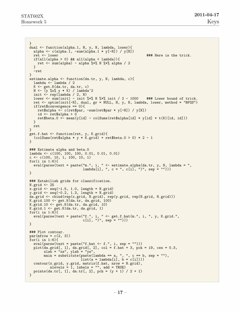
Nasty trick: There are several algorithms can handle optimization with complicated con-

straints. In R, constrOptim() implements a barier algorithm (Lange 2001), but this function

is not quite easy to manupilate for large number of constraints. In general, there is a nasty

trick I play around with this kind of problems. When I plug in optim() an objective func-

tion, I add some checking points inside the objective function to fool optim(). For example, I

usually use if(...)...else... to return a ±Inf (dependent on minimizing or maximizing)

to fool optim() if the new/next estimates (generated by the optimizing code) are out of any

constraint. At the end, if the optim() reports convergence, then the problem may be solved,

otherwise it is definitely NOT ok.

If the problem has some signals showing the monotonicity of objective function, then we

can just add or substract (dependent on minimizing or maximizing) some arbitrarily values

to the initial objective value. In the following, I use lower as the lowest (initial) objective

value with subjstraction 1000 (choose any positive whatever you like) from it. Then, I input

it as an argument to adjust the objective function. Can this trick fail? Yes, but for this

problem, it converges.

– 15 –

STAT602XHomework 5

2011-04-17

Keys

−1.5 −1.0 −0.5 0.0 0.5 1.0

0.0

0.5

1.0

λ = 100, c = 100

xs

ys

−1.5 −1.0 −0.5 0.0 0.5 1.0

0.0

0.5

1.0

λ = 100, c = 10

xs

ys

−1.5 −1.0 −0.5 0.0 0.5 1.0

0.0

0.5

1.0

λ = 100, c = 1

xs

ys

−1.5 −1.0 −0.5 0.0 0.5 1.0

0.0

0.5

1.0

λ = 0.01, c = 100

xs

ys

−1.5 −1.0 −0.5 0.0 0.5 1.0

0.0

0.5

1.0

λ = 0.01, c = 10

xs

ys

−1.5 −1.0 −0.5 0.0 0.5 1.0

0.0

0.5

1.0

λ = 0.01, c = 1

xs

ys

R Code (Warning: this may have some bugs)da <- read.table("synth.tr", sep = "", quote = "", header = TRUE)da.tr <- cbind(da$xs, da$ys)y <- da$yc * 2 - 1N <- length(y)

get.K <- function(da.tr.i, da.tr.j, c = 1){N.i <- nrow(da.tr.i)N.j <- nrow(da.tr.j)K <- matrix(0, nrow = N.i, ncol = N.j)for(i in 1:N.i){for(j in 1:N.j){K[i, j] <- exp(-c * sum((da.tr.i[i,] - da.tr.j[j,])^2))

}}K

– 16 –

STAT602XHomework 5

2011-04-17

Keys

}dual <- function(alpha.1, H, y, N, lambda, lower){alpha <- c(alpha.1, -sum(alpha.1 * y[-N]) / y[N])ret <- lower ### Here is the trick.if(all(alpha > 0) && all(alpha < lambda)){ret <- sum(alpha) - alpha %*% H %*% alpha / 2

}-ret

}estimate.alpha <- function(da.tr, y, N, lambda, c){lambda <- lambda / 2K <- get.K(da.tr, da.tr, c)H <- (y %o% y * K) / lambda^2init <- rep(lambda / 2, N)lower <- sum(init) - init %*% H %*% init / 2 - 1000 ### Lower bound of trick.ret <- optim(init[-N], dual, gr = NULL, H, y, N, lambda, lower, method = "BFGS")if(ret$convergence == 0){ret$alpha <- c(ret$par, -sum(ret$par * y[-N]) / y[N])id <- ret$alpha > 0ret$beta.0 <- mean(y[id] - colSums(ret$alpha[id] * y[id] * t(K)[id, id]))

}ret

}get.f.hat <- function(ret, y, K.grid){(colSums(ret$alpha * y * K.grid) + ret$beta.0 > 0) * 2 - 1

}

### Estimate alpha and beta.0lambda <- c(100, 100, 100, 0.01, 0.01, 0.01)c <- c(100, 10, 1, 100, 10, 1)for(i in 1:6){eval(parse(text = paste("m.", i, " <- estimate.alpha(da.tr, y, N, lambda = ",

lambda[i], ", c = ", c[i], ")", sep = "")))}

### Estabilish grids for classification.N.grid <- 25x.grid <- seq(-1.5, 1.0, length = N.grid)y.grid <- seq(-0.2, 1.3, length = N.grid)da.grid <- cbind(rep(x.grid, N.grid), rep(y.grid, rep(N.grid, N.grid)))K.grid.100 <- get.K(da.tr, da.grid, 100)K.grid.10 <- get.K(da.tr, da.grid, 10)K.grid.1 <- get.K(da.tr, da.grid, 1)for(i in 1:6){eval(parse(text = paste("f.", i, " <- get.f.hat(m.", i, ", y, K.grid.",

c[i], ")", sep = "")))}

### Plot contour.par(mfrow = c(2, 3))for(i in 1:6){eval(parse(text = paste("f.hat <- f.", i, sep = "")))plot(da.grid[, 1], da.grid[, 2], col = f.hat + 3, pch = 19, cex = 0.3,

xlab = "xs", ylab = "ys",main = substitute(paste(lambda == a, ", ", c == b, sep = ""),

list(a = lambda[i], b = c[i])))contour(x.grid, y.grid, matrix(f.hat, nrow = N.grid),

nlevels = 1, labels = "", add = TRUE)points(da.tr[, 1], da.tr[, 2], pch = (y + 1) / 2 + 1)

}

– 17 –

STAT602XHomework 5

2011-04-17

Keys

Total: 80 pts (Q20: 15, Q21: 10, Q22: 10, Q23: 15, Q24: 10, Q25: 10, Q26: 10). Any resonable

solutions are acceptable.

– 18 –