STAT2201

Analysis ofEngineering & Scientific Data

Condensed Course Notes.

Semester 1, 2017.

Last Edited: April 23, 2017Contains All Units 1 – 10

These condensed notes summarise definitions, procedures, theorems and results relevant forSTAT2201. Further material is available in the course book, Applied Statistics and Probability forEngineers” by D. C. Montgomery and G. C. Runger, [MonRun2014] and on the course web-site:

https://courses.smp.uq.edu.au/STAT2201/2017a .It is recommended to bring printouts of these notes to course lectures and tutorials.

c© School of Mathematics and Physics, The University of Queensland, Brisbane QLD 4072, Australia.

Contains materials and contributions developed by Yoni Nazarathy, Melanie Robertson-Dean and Hayden Klok.

1

About:

These condensed course notes are designed as an aid for lecture participation, tutorial participa-tion, assignment preparation and reading of the course book. The course is structured with 10 studyunits, 1–10. It is recommended to attend lecture and tutorial sessions with printouts of the notes forthe relevant unit as well as earlier units. For example, when attending lectures associated with unit5, bring print outs of at least units 1–5. These will help you follow the lectures and tutorials. See thecourse website for a detailed lecture and tutorial schedule.

A major goal of this course is to enable students to “talk the language” of probability and statistics.This includes understanding of terms such as probability, events, random variables, distributions,means, moments, estimation, confidence intervals, hypothesis tests, regression and much more. Eachof these concepts on its own, entails a variety of associated concepts, results, formulas and properties.Hence the volume of terms and concepts is rather large in comparison to the course duration. Thisdocument’s goal is to alleviate hardships associated with this, by giving a succinct description of thecontent.

1

The course units are as follows:

Unit 1 – IntroductionAn overview of the terms: probability, statistics, data-analysis, data science, inference, experi-mentation, deterministic models, stochastic models, statistical models. Introduction to the Julialanguage and an overview of alternatives. Simulation examples.

Unit 2 – Probability and Monte CarloProbability spaces, outcomes and events. Operations on events as subsets of the sample space.The meaning of probabilistic statements. Independence. Conditional probability and the law oftotal probability. Pseudorandom number generation and Monte Carlo in a bit more depth.

Unit 3 – DistributionsRandom variables. Mathematical description of the distribution of discrete and continuousrandom variables. Probability mass functions, probability density functions and cumulative dis-tribution functions. Expectation, mean, variance, standard deviation and moments. Quantiles.Discrete uniform and binomial distributions. Uniform (continuous), exponential and normal(Gaussian) distributions. Using the normal distribution table.

Unit 4 – Joint DistributionsBivariate and multivariate probability distributions. Marginal distributions. Covariance and cor-relation. Independent random variables. Expectations of functions of several random variables.Means and variance of sums and linear combinations of random variables.

Unit 5 – Descriptive StatisticsStatistics as functions of a sample: sample mean, sample variance and common summarisingfunctions. Box plots. Constructing histograms. Samples with two or more variables. Samplecorrelation. Scatter plots. Time series. Cumulative plots including probability plots.

Unit 6 – Statistical Inference IdeasRandom samples. Point estimates. The sampling distribution of a statistic. The central limittheorem. Confidence interval idea. Confidence intervals for the mean when the variance is knownor for large samples. Prediction intervals. Hypothesis test ideas. Types of error in hypothesistesting. P-value. A general procedure for hypothesis testing.

Unit 7 – Single Sample InferenceThe t-distribution. Confidence intervals for the mean of a normal distribution when the varianceis not known. Hypothesis tests for the mean of a normal distribution when the variance is notknow (the t-test).

Unit 8 – Two Sample InferenceConfidence intervals and hypothesis tests for the difference in means of a normal distributionwhen the variance is not known (the two sample t-test). Pooled sample variance. Approximationswhen population variances are assume difference. Understanding model assumptions.

Unit 9 – Linear RegressionFitting a line through points using least squares. The meaning of linear statistical models.Simple linear regression (slope and intercept). Residual analysis. Properties of the leas squareestimators. R squared. Hypothesis tests for regression. A brief discussion of transformations.Logistic regression.

Unit 10 – What more is thereA survey of basic tools from a first statistics course not covered here: Chi-square tests for good-ness of fit and independence, non-parameteric tests for fitting distributions, analysis of variance(ANOVA), experimental design, multi-variable regression, principal components analysis, gener-alized linear models, time-series analysis, survival analysis, reliability modelling, queueing theoryand related stochastic models dealing with random processes.

2

1 Introduction and Julia

ã Probability is a measure of the likelihood of an event occurring and Probability theory is abranch of mathematics dealing with probabilities.

ã Statistics is the science of data and involves probability due to: (i) The random nature ofsampling data. (ii) Probability theory is useful for devising statistical models and techniques.

ã Data Science is an emerging field, combining statistics, big-data, machine learning andcomputational techniques.

ã There are thousands of active statistics researchers around the world and tens of thousandsstatisticians and data scientists.

ã Within the field of statistics, there are specialisations in biostatistics, mathematical statis-tics, non-parametric statistics, machine learning, linear models, survival analysis,Baysian statistics, Geo-spatial statistics and many more.

ã Within the field of Probability theory, there are more theoretical researchers dealing withabstract mathematical models as well as researchers and practitioners dealing with appliedprobability, also related to stochastic operations research. Applied probability containsreliability theory, biological population models, inventory theory, queueing theoryand a few other related fields.

ã Data analysis is the process of curating, organising and analysing data sets to make inferences.

ã Statistical Inference is the process of making inferences about population parameters(often never fully observed) based on observations collected as part of samples.

ã A statistic or summary statistic is a quantity calculated from a sample.

ã Data can be collected and analysed through a retrospective study, observational study,designed experiments or a combination.

ã When collecting data, the notion of time sometimes plays a key role.

ã A deterministic model of a physical, chemical, biological, financial or related scenario doesnot involve any randomness.

ã A stochastic model contains built in randomness. Different realisations (runs) of the modelyield different outcomes or trajectories.

ã A statistical model is a stochastic model of suited directly for inference.

ã Some models are mechanistic and are based on basic physical (or related) principles. Othermodels are empirical and are of the more “black box” or “grey box” type. Statistical modelsare often empirical, but a statistical model can be incorporated with a mechanistic model.

ã Simulation (in the context of mathematical models) is the process of generating observations/-trajectories/outcomes using a computer based on a model. In case of a stochastic or statisticalmodel, this is called Monte Carlo (famous casino) simulation and uses random numbers gen-erated on the computer (often pseudorandom numbers).

ã An example of a pseudorandom sequence is the classic linear congruential generator:

zn+1 = (a zn + c) mod m,

where z0 is some initial seed and a, c and m are parameters. For example a known “good” setof parameters is,

a = 69069, c = 1, m = 232.

3

ã In this course we will use the Julia programming language, v0.5.0 through uq.juliabox.com.

ã There are dozens of possible software packages and languages for statistics, data-analysis, data-science and scientific computing. Here is a partial list:

1. R - Has become the language of choice for the statistics community.

2. Matlab - Often the language of choice for engineering, especially, IEEE systems and con-trol.

3. Octave - An open source alternative to Matlab.

4. Scilab - Another open source alternative to Matlab.

5. Mathematica - A general purpose mathematics, data-science, numerical computing plat-form. Made it’s name with superb symbolic computation abilities. Very powerful in manyother domains.

6. Maple - Similar to Mathematica with strong symbolic capabilities.

7. Wolfram Alpha Pro - A more user friendly version of Mathematica, uses more naturallanguage and less programming.

8. Python (including NumPy) - Often the language of choice for Data Science.

9. General programming languages – C/C++, Java, C#, Go, Swift, Fortran (to namea few)– Not specifically tailored for scientific computing and data-analysis, although theyoften have many libraries.

10. Languages (mostly) from the past – Lisp, Smalltalk, Pascal – Influenced current lan-guages.

11. Javscript – Runs on web-browser (together with html and css). Not really tailored forscientific computation.

12. PHP, NodesJS – Server side for supporting web-pages. Not really tailored for scientificcomputation.

13. Excel (and similar such as Apple’s Numbers) - General spreadsheet software. Oftenpowerful enough for quick simple computations or much more. May require plug-in languagesuch as Visual Basic in Excel for specific macros.

14. Excel like Statistics packages - SPSS and Minitab. More geared towards observations(rows) and variables (columns) than Excel and often yield very easy to use output ofcommon statistical procedures.

15. Specific Statistics and Machine Learning software and packages – E.g. Win-BUGS, H20, Google Tensor Flow and much more.

16. Specific civil, mechanical and aerospace modelling languages and software pack-ages – You will use these in your career.

17. Latex - The typesetting language we use for these notes. Not a scientific computinglanguage.

18. SQL - A Database Query Language for relational databases. Not a scientific computinglanguage.

19. Assembly, LLVM – Low level (not for us).

20. Julia - A relatively new (still in version 0.5.0) open sourced general purpose scientificcomputing language. Similar in nature to Python and Matlab, but strongly typed and JustIn Time compiled hence very fast in execution.

ã We are using iJulia, a Jupyter style notebook running on a web browser through JuliaBox.Current alternatives include a local install of iJulia, the Julia REPL (command line), a plug-ininto the Atom Editor - we won’t use these.

4

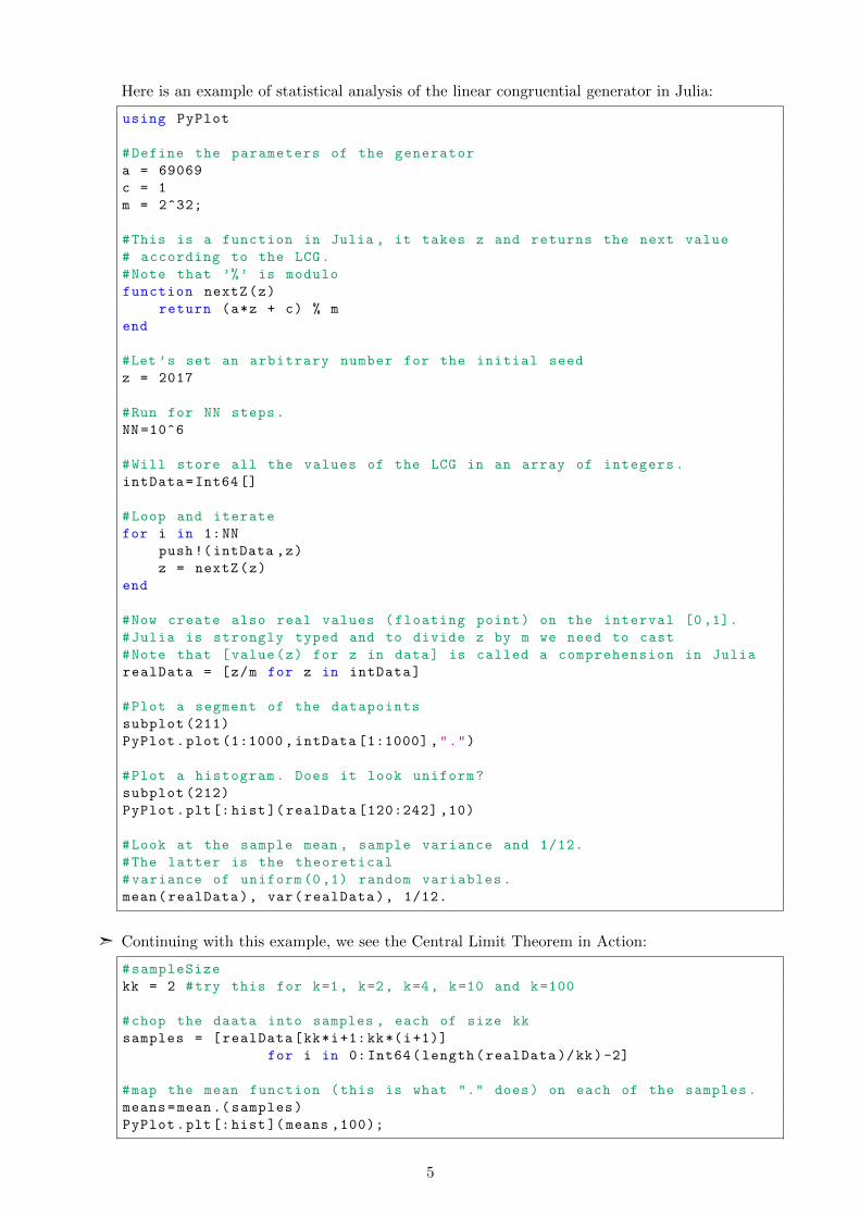
Here is an example of statistical analysis of the linear congruential generator in Julia:

using PyPlot

#Define the parameters of the generator

a = 69069

c = 1

m = 2^32;

#This is a function in Julia , it takes z and returns the next value

# according to the LCG.

#Note that ’%’ is modulo

function nextZ(z)

return (a*z + c) % m

end

#Let ’s set an arbitrary number for the initial seed

z = 2017

#Run for NN steps.

NN =10^6

#Will store all the values of the LCG in an array of integers.

intData=Int64[]

#Loop and iterate

for i in 1:NN

push!(intData ,z)

z = nextZ(z)

end

#Now create also real values (floating point) on the interval [0 ,1].

#Julia is strongly typed and to divide z by m we need to cast

#Note that [value(z) for z in data] is called a comprehension in Julia

realData = [z/m for z in intData]

#Plot a segment of the datapoints

subplot (211)

PyPlot.plot (1:1000 , intData [1:1000] ,".")

#Plot a histogram. Does it look uniform?

subplot (212)

PyPlot.plt[:hist]( realData [120:242] ,10)

#Look at the sample mean , sample variance and 1/12.

#The latter is the theoretical

#variance of uniform (0,1) random variables.

mean(realData), var(realData), 1/12.

ã Continuing with this example, we see the Central Limit Theorem in Action:

#sampleSize

kk = 2 #try this for k=1, k=2, k=4, k=10 and k=100

#chop the daata into samples , each of size kk

samples = [realData[kk*i+1:kk*(i+1)]

for i in 0: Int64(length(realData )/kk)-2]

#map the mean function (this is what "." does) on each of the samples.

means=mean.( samples)

PyPlot.plt[:hist](means ,100);

5

2 Probability and Monte Carlo

ã An experiment that can result in different outcomes, even though it is repeated in the samemanner every time, is called a random experiment.

ã The set of all possible outcomes of a random experiment is called the sample space of theexperiment, and is denoted as Ω.

• A sample space is discrete if it consists of a finite or countable infinite set of outcomes.

• A sample space is continuous if it contains an interval (either finite or infinite) of realnumbers, vectors or similar objects.

ã An event is a subset of the sample space of a random experiment.

• The union of two events is the event that consists of all outcomes that are contained ineither of the two events or both. We denote the union as E1 ∪ E2.

• The intersection of two events is the event that consists of all outcomes that are containedin both of the two events. We denote the intersection as E1 ∩ E2.

• The complement of an event in a sample space is the set of outcomes in the sample spacethat are not in the event. We denote the complement of the event E as E. The notationEC is also used in other literature to denote the complement. Note that E ∪ E = Ω.

ã Two events, denoted E1 and E2 are mutually exclusive if: E1 ∩E2 = ∅ where ∅ is called theempty set or null event.

ã A collection of events, E1, E2, . . . , Ek is said to be mutually exclusive if for all pairs,

Ei ∩ Ej = ∅.

ã The definition of the complement of an event implies that: (Ec)c = E.

ã The distributive law for set operations implies that

(A ∪B) ∩ C = (A ∩ C) ∪ (B ∩ C) and (A ∩B) ∪ C = (A ∪ C) ∩ (B ∪ C).

ã DeMorgan’s laws imply that

(A ∪B)c = Ac ∩Bc and (A ∩B)c = Ac ∪Bc.

ã Union and intersection are commutative operations: A∩B = B∩A and A∪B = B∪A.

ã Probability is used to quantify the likelihood, or chance, that an outcome of a random experi-ment will occur.

ã Whenever a sample space consists of a finite number N of possible outcomes, each equallylikely, the probability of each outcome is 1/N .

ã For a discrete sample space, the probability of an event E, denoted as P (E), equals the sumof the probabilities of the outcomes in E.

ã If Ω is the sample space and E is any event in a random experiment,

(1) P (Ω) = 1.

(2) 0 ≤ P (E) ≤ 1.

(3) For two events E1 and E2 with E1 ∩ E2 = ∅ (disjoint),

P (E1 ∪ E2) = P (E1) + P (E2)

6

(4) P (Ec) = 1− P (E).

(5) P (∅) = 0.

ã The probability of event A or event B occurring is,

P (A ∪B) = P (A) + P (B)− P (A ∩B).

ã If A and B are mutually exclusive events,

P (A ∪B) = P (A) + P (B)

ã For a collection of mutually exclusive events,

P (E1 ∪ E2 ∪ · · · ∪ Ek) = P (E1) + P (E2) + . . . P (Ek)

ã The probability of an event B under the knowledge that the outcome will be in event A isdenoted P (B |A) and is called the conditional probability of B given A.

ã The conditional probability of an event B given an event A, denoted as P (B |A), is

P (B |A) =P (A ∩B)

P (A)for P (A) > 0.

ã The multiplication rule for probabilities is: P (A ∩B) = P (B |A)P (A) = P (A |B)P (B).

ã For an event B and a collection of mutual exclusive events, E1, E2, . . . , Ek where their union isΩ. The law of total probability yields,

P (B) = P (B ∩ E1) + P (B ∩ E2) + · · ·+ P (B ∩ Ek)= P (B | E1)P (E1) + P (B | E2)P (E2) + · · ·+ P (B | Ek)P (Ek).

ã Two events are independent if any one of the following equivalent statements is true:

(1) P (A |B) = P (A).

(2) P (B |A) = P (B).

(3) P (A ∩B) = P (A)P (B).

Observe that independent events and mutually exclusive events, are completely differentconcepts. Don’t confuse these concepts.

ã For multiple events E1, E2, . . . , En are independent if and only if for any subset of these events

P (Ei1 ∩ Ei2 ∩ · · · ∩ Eik) = P (Ei1) P (Ei2) . . . P (Eik).

ã A pseudorandom sequence is a sequence of numbers U1, U2, . . . with each number, Uk depend-ing on the previous numbers Uk−1, Uk−2, . . . , U1 through a well defined functional relationshipand similarly U1 depending on the seed U0. Hence for any seed, U0, the resulting sequenceU1, U2, . . . is fully defined and repeatable. A pseudorandom sequence often lives within a dis-crete domain as 0, 1, . . . , 264 − 1. It can then be normalised to floating point numbers with,

Rk =Uk

264 − 1.

ã A good pseudorandom sequence has the following attributes among others:

1. It is quick and easy to compute the next element in the sequence.

2. The sequence of numbers R1, R2, . . . resembles properties as an i.i.d. sequence of uni-form(0,1) random variables (i.i.d. is defined in Unit 4).

ã Computer simulation of random experiments is called Monte Carlo and is typically carried outby setting the seed to either a reproducible value or an arbitrary value such as system time.

ã Random experiments may be replicated on a computer using Monte Carlo simulation.

7

3 Distributions

ã A random variable X is a numerical (integer, real, complex, vector etc.) summary of theoutcome of the random experiment. The range or support of the random variable is the setof possible values that it may take. Random variables are usually denoted by capital letters.

ã A discrete random variable is an integer/real-valued random variable with a finite (or count-ably infinite) range.

ã A continuous random variable is a real valued random variable with an interval (either finiteor infinite) of real numbers for its range.

ã The probability distribution of a random variable X is a description of the probabilitiesassociated with the possible values of X. There are several common alternative ways to describethe probability distribution, with some differences between discrete and continuous randomvariables.

ã While not the most popular in practice, a unified way to describe the distribution of any scalarvalued random variable X (real or integer) is the cumulative distribution function,

F (x) = P (X ≤ x).

ã It holds that

(1) 0 ≤ F (x) ≤ 1.

(2) limx→−∞ F (x) = 0.

(3) limx→∞ F (x) = 1.

(4) If x ≤ y, then F (x) ≤ F (y). That is, F (·) is non-decreasing.

ã Distributions are often summarised by numbers such as the mean, µ, variance, σ2, or mo-ments. These numbers, in general do not identify the distribution, but hint at the generallocation, spread and shape.

ã The standard deviation of X is σ =√σ2 and is particularly useful when working with the

Normal distribution.

ã Given a discrete random variable X with possible values x1, x2, . . . , xn, the probability massfunction of X is,

p(x) = P (X = x).

Note: In [MonRun2014] and many other sources, the notation used is f(x) (as a pdf of acontinuous random variable).

ã A probability mass function, p(x) satisfies:

(1) p(xi) ≥ 0.

(2)

n∑i=1

p(xi) = 1.

ã The cumulative distribution function of a discrete random variable X, denoted as F (x), is

F (x) =∑xi≤x

p(xi).

ã P (X = xi) can be determined from the jump at the value of x. More specifically

p(xi) = P (X = xi) = F (xi)− limx↑xi

F (xi).

8

ã The mean or expected value of a discrete random variable X, is

µ = E(X) =∑x

x p(x).

ã The expected value of h(X) for some function h(·) is:

E[h(X)

]=∑x

h(x) p(x).

ã The k’th moment of X is,

E(Xk) =∑x

xk p(x).

ã The variance of X, is

σ2 = V (X) = E(X − µ)2 =∑x

(x− µ)2 p(x) =∑x

x2 p(x)− µ2.

ã A random variable X has a discrete uniform distribution if each of the n values in its range,x1, x2, . . . , xn, has equal probability. I.e.

p(xi) = 1/n.

ã Suppose that X is a discrete uniform random variable on the consecutive integers a, a + 1, a +2, . . . , b, for a ≤ b. The mean and variance of X are

E(X) =b+ a

2and V (X) =

(b− a+ 1)2 − 1

12.

ã The setting of n independent and identical Bernoulli trials is as follows:

(1) There are n trials.

(1) The trials are independent.

(2) Each trial results in only two possible outcomes, labelled as “success” and “failure”.

(3) The probability of a success in each trial denoted as p is the same for all trials.

ã The random variable X that equals the number of trials that result in a success is a binomialrandom variable with parameters 0 ≤ p ≤ 1 and n = 1, 2, . . . . The probability mass functionof X is

p(x) =

(n

x

)px(1− p)n−x, x = 0, 1, . . . , n.

ã Useful to remember from algebra: the binomial expansion for constants a and b is

(a+ b)n =n∑k=0

(n

k

)akbn−k.

ã If X is a binomial random variable with parameters p and n, then,

E(X) = n p and V (X) = n p (1− p).

9

ã Given a continuous random variable X, the probability density function (pdf) is a function,f(x) such that,

(1) f(x) ≥ 0.

(2) f(x) = 0 for x not in the range.

(3)∞∫−∞

f(x) dx = 1.

(4) For small ∆x, f(x) ∆x ≈ P (X ∈ [x, x+ ∆x)).

(5) P (a ≤ X ≤ b) =b∫af(x)dx = area under f(x) from a to b.

ã Given the PDF, f(x) we can get the CDF as follows:

F (x) = P (X ≤ x) =

x∫−∞

f(u)du for −∞ < x <∞.

ã Given the CDF, F (x) we can get the PDF:

f(x) =d

dxF (x).

ã The mean or expected value of a continous random variable X, is

µ = E(X) =

∞∫−∞

x f(x)dx.

ã The expected value of h(X) for some function h(·) is:

E[h(X)

]=

∞∫−∞

h(x)f(x) dx.

ã The k’th moment of X is,

E(Xk) =

∞∫−∞

xk f(x) dx.

ã The variance of X, is

σ2 = V (X) =

∞∫−∞

(x− µ)2f(x)dx =

∫ ∞−∞

x2f(x) dx− µ2.

ã A continuous random variable X with probability density function

f(x) =1

b− a, a ≤ x ≤ b.

is a continuous uniform random variable or “uniform random variable” for short.

ã If X is a continuous uniform random variable over a ≤ x ≤ b, the mean and variance are:

µ = E(X) =a+ b

2and σ2 = V (X) =

(b− a)2

12.

10

ã A random variable X with probability density function

f(x) =1

σ√

2πe

−(x−µ)2

2σ2 , −∞ < x <∞,

is a normal random variable with parameters µ where −∞ < µ < ∞, and σ > 0. For thisdistribution, the parameters map directly to the mean and variance,

E(X) = µ and V (X) = σ2.

The notation N(µ, σ2) is used to denote the distribution. Note that some authors and softwarepackages use σ for the second parameter and not σ2.

ã A normal random variable with a mean and variance of:

µ = 0 and σ2 = 1

is called a standard normal random variable and is denoted as Z. The cumulative distri-bution function of a standard normal random variable is denoted as

Φ(z) = FZ(z) = P (Z ≤ z),

and is tabulated in a table.

ã It is very common to compute P (a < X < b) for X ∼ N(µ, σ2). This is the typical way:

P (a < X < b) = P (a− µ < X − µ < b− µ)

= P(a− µ

σ<X − µσ

<b− µσ

)= P

(a− µσ

< Z <b− µσ

)= Φ

(b− µσ

)− Φ

(a− µσ

).

We get:

FX(b)− FX(a) = FZ

(b− µσ

)− FZ

(a− µσ

).

ã The exponential distribution with parameter λ > 0 is given by the survival function,

F (x) = 1− F (x) = P (X > x) = e−λx.

ã The random variable X that equals the distance between successive events from a Poisson processwith mean number of events per unit interval λ > 0.

ã The probability density function of X is

f(x) = λe−λx for 0 ≤ x <∞.

Note that sometimes a different parameterisation, θ = 1/λ is used (e.g. in the Julia Distributionspackage).

ã The mean and variance are:

µ = E(X) =1

λand σ2 = V (X) =

1

λ2

ã The exponential distribution is the only continuous distribution with range [0,∞) exhibiting thelack of memory property. For an exponential random variable X,

P (X > t+ s |X > t) = P (X > s).

ã Monte Carlo simulation makes use of methods to transform a uniform random variable in amanner where it follows an arbitrary given given distribution. One example of this is if U ∼Uniform(0, 1) then X = − 1

λ log(U) is exponentially distributed with parameter λ.

11

4 Joint Probability Distributions

ã A joint probability distribution of two random variables is also referred to as bivariate prob-ability distribution.

ã A joint probability mass function for discrete random variables X and Y , denoted aspXY (x, y), satisfies the following properties:

(1) pXY (x, y) ≥ 0 for all x, y.

(2) pXY (x, y) = 0 for (x, y) not in the range.

(3)∑∑

pXY (x, y) = 1, where the summation is over all (x, y) in the range.

(4) pXY (x, y) = P (X = x, Y = y).

ã A joint probability density function for continuous random variables X and Y , denoted asfXY (x, y), satisfies the following properties:

(1) fXY (x, y) ≥ 0 for all x, y.

(2) fXY (x, y) = 0 for (x, y) not in the range.

(3)∞∫−∞

∞∫−∞

fXY (x, y) dx dy = 1.

(4) For small ∆x, ∆y: fXY (x, y) ∆x∆y ≈ P(

(X,Y ) ∈ [x, x+ ∆x)× [y, y + ∆ y)).

(5) For any region R of two-dimensional space,

P(

(X,Y ) ∈ R)

=∫∫R

fXY (x, y) dx dy.

ã A joint probability density function can also be defined for n > 2 random variables (as canbe a joint probability mass function). The following needs to hold:

(1) fX1X2...Xp(x1, x2, . . . , xn) ≥ 0.

(2)∞∫−∞

∞∫−∞· · ·

∞∫−∞

fX1X2...Xp(x1, x2, . . . , xn)dx1 dx2 . . . dxn = 1.

ã Most of the concepts in this section, carry over from bivariate to general multivariate distribu-tions (n > 2).

ã The marginal distributions of X and Y as well as conditional distributions of X given aspecific value Y = y and vice versa can be obtained from the joint distribution.

ã If the random variables X and Y are independent, then fXY (x, y) = fX(x) fY (y) and similarlyin the discrete case.

ã The expected value of a function of two random variables is:

E[h(X,Y )

]=

∫∫h(x, y)fXY (x, y) dx dy for X,Y continuous.

ã The covariance is a common measure of the relationship between two random variables (sayX and Y ). It is denoted as cov(X,Y ) or σXY , and is given by:

σXY = E[(X − µX)(Y − µY )

]= E(XY )− µXµY .

ã The covariance of a random variable with itself is its variance.

12

ã The correlation between the random variables X and Y , denoted as ρXY , is

ρXY =cov(X,Y )√V (X)V (Y )

=σXYσXσY

.

ã For any two random variables X and Y , −1 ≤ ρXY ≤ 1.

ã If X and Y are independent random variables, σXY = 0 and ρXY = 0. The opposite case does notalways hold: In general ρXY = 0 does not imply independence. But for jointly Normal randomvariables it does. In any case, if ρXY = 0 then the random variables are called uncorrelated.

ã When considering several random variables, it is common to consider the (symmetric) Covari-ance Matrix, Σ with Σi,j = cov(Xi, Xj).

ã The probability density function of a bivariate normal distribution is

fXY (x, y;σX , σY , µX , µY , ρ) =1

2πσXσY√

1− ρ2

× exp

−1

2(1− ρ2)

[(x− µX)2

σ2X− 2ρ(x− µX)(y − µY )

σXσY+

(y − µY )2

σ2Y

]for −∞ < x <∞ and −∞ < y <∞,with parameters σX > 0, σY > 0, −∞ < µX <∞, −∞ < µY <∞, and −1 < ρ < 1.

ã Given random variables X1, X2, . . . , Xn and constants c1, c2, . . . , cn, the (scalar) linear combi-nation

Y = c1X1 + c2X2 + · · ·+ cnXn

is often a random variable of interest.

ã The mean of the linear combination is the linear combination of the means,

E(Y ) = c1E(X1) + c2E(X2) + · · ·+ cnE(Xn).

This holds even if the random variables are not independent.

ã The variance of the linear combination is as follows:

V (Y ) = c21V (X1) + c22V (X2) + · · ·+ c2nV (Xn) + 2∑i<j

∑cicjcov(Xi, Xj)

ã If X1, X2, . . . , Xn are independent (or even if they are just uncorrelated).

V (Y ) = c21V (X1) + c22V (X2) + · · ·+ c2nV (Xn).

ã In case the random variables X1, . . . , Xn were jointly Normal then, Y ∼ Normal(E(Y ), V (Y )

).

That is, linear combinations of Normal random variables remain Normally distributed.

ã A collection of random variables, X1, . . . , Xn is said to be i.i.d., or independent and iden-tically distributed if they are mutually independent and identically distributed. This meansthat the (n - dimensional) joint probability density is a product of the individual densities.

ã In the context of statistics, a random sample is often modelled as an i.i.d. vector of randomvariables. X1, . . . , Xn.

ã An important linear combination associated with a random sample is the sample mean:

X =

∑ni=1Xi

n=

1

nX1 +

1

nX2 + . . .+

1

nXn.

ã If Xi has mean µ and variance σ2 then sample mean (of an i.i.d. sample) has,

E(X) = µ, V (X) =σ2

n.

13

5 Descriptive Statistics

ã Descriptive statistics deals with summarizing data using numbers, qualitative summaries,tables and graphs.

ã Here are some types of data configurations:

1. Single sample: x1, x2, . . . , xn.

2. Single sample over time (time series): xt1 , xt2 , . . . , xtn with t1 < t2 < . . . < tn.

3. Two samples: x1, . . . , xn and y1, . . . , ym.

4. Generalizations from two samples to k samples (each of potentially different sample size,n1, . . . , nk).

5. Observations in tuples: (x1, y1), (x2, y2), . . . , (xn, yn).

6. Generalizations from tuples to vector observations (each vector of length `),

(x11, . . . , x`1), . . . , (x

1n, . . . , x

`n).

ã Individual variables may be categorical or numerical. Categorical variables (taking valuesin one of several categories) may be ordinal meaning that they be sorted (e.g. “a”, “b”, “c”,“d”), or not (e.g. “cat”, “dog”, “fish”).

ã A statistic is a quantity computed from a sample (assume here a single sample x1, . . . , xn).Here are very common and useful statistics:

1. The sample mean: x =x1 + · · ·+ xn

n=

n∑i=1

xi

n.

2. The sample variance: s2 =

n∑i=1

(xi − x)2

n− 1=

n∑i=1

x2i − nx2

n− 1.

3. The sample standard deviation: s =√s2.

4. Order statistics work as follows: Sort the sample to obtain the sequence of sorted ob-servations, denoted x(1), . . . , x(n) where, x(1) ≤ x(2) ≤ . . . ≤ x(n). Some common orderstatistics:

(a) The minimum min(x1, . . . , xn) = x(1).

(b) The maximum max(x1, . . . , xn) = x(n).

(c) The median

median =

x(n+1

2) if n is odd,

12

(x(n

2) + x(n

2+1)

)if n is even.

Note that the median is the 50’th percentile and the 2nd quartile (see below).

(d) The q th quantile (q ∈ [0, 1]) or alternatively the p = 100q percentile (measured inpercents instead of a decimal), is the observation such that p percent of the observationsare less than it and (1−p) percent of the observations are greater than it. In cases (as istypical) that there is not such a precise observation, it is a linear interpolation betweentwo neighbouring observations (as is done for the median when n is even). In termsof order statistics, the q th quantile is approximately (not taking linear interpolationsinto account) x([q∗n]). Here [z] denotes the nearest integer in 1, . . . , n to z.

(e) The first quartile, denoted Q1 is the 25th percentile. The second quartile (Q2) isthe median. The third quartile, denoted Q3 is the 75th percentile. Thus half of theobservations lie between Q1 and Q3. In other words, the quartiles break the sampleinto 4 quarters. The difference Q3−Q1 is the interquartile range.

(f) The sample range is x(n) − x(1).

14

ã Constructing a Histogram (Equal Bin Widths)

(1) Label the bin (class interval) boundaries on a horizontal scale.

(2) Mark and label the vertical scale with frequencies or counts.

(3) Above each bin, draw a rectangle where height is equal to the frequency (or count).

ã A Kernel Density Estimate (KDE) is a way to construct a Smoothed Histogram. Whileconstruction is not as straightforward as steps (1)–(3) above, automated tools can be used.

ã Both the histogram and the KDE are not unique in the way they summarize data. With thesemethods, different settings (e.g. number of bins in histograms or bandwidth in a KDE) mayyield different representations of the same data set. Nevertheless, they are both very common,sensible and useful visualisations of data.

ã The box plot is a graphical display that simultaneously describes several important features ofa data set, such as centre, spread, departure from symmetry, and identification of unusualobservations or outliers. It is often common to plot several box plots next to each other forcomparison.

ã An anachronistic, but useful way for summarising small data-sets is the stem and leaf diagram.

ã In a cumulative frequency plot the height of each bar is the total number of observationsthat are less than or equal to the upper limit of the bin.

ã The Empirical Cumulative Distribution Function (ECDF) is,

F (x) =1

n

n∑i=1

1xi ≤ x.

Here 1· is the indicator function. The ECDF is a function of the data, defined for all x.

ã Given a candidate distribution with CDF F (x), a probability plot is a plot of the ECDF(or sometimes just it’s jump points) with the y-axis stretched by the inverse of the CDF F−1(·).The monotonic transformation of the y-axis is such that if the data comes from the candidateF (x), the points would appear to lie on a straight line. Names of variations of probability plotsare the P-P plot and Q-Q plot (these plots are similar to the probability plot). A very commonprobability plot is the Normal probability plot where the candidate distribution is taken tobe Normal(x, s2).

ã The Normal probability plot can be useful in identifying distributions that are symmetric butthat have tails that are “heavier” or “lighter” than the Normal.

ã A time series plot is a graph in which the vertical axis denotes the observed value of thevariable and the horizontal axis denotes time.

ã A scatter diagram is constructed by plotting each pair of observations with one measurementin the pair on the vertical axis of the graph and the other measurement in the pair on thehorizontal axis.

ã The sample correlation coefficient rxy is an estimate for the correlation coefficient, ρ, pre-sented in the previous unit:

rxy =

n∑i=1

(yi − y)(xi − x)√n∑i=1

(yi − y)2n∑i=1

(xi − x)2

.

15

6 Statistical Inference Ideas

ã Statistical Inference is the process of forming judgements about the parameters of a pop-ulation, typically on the basis of random sampling.

ã The random variables X1, X2, . . . , Xn are an (i.i.d.) random sample of size n if

(a) the Xi’s are independent random variables and

(b) every Xi has the same probability distribution.

ã A statistic is any function of the observations in a random sample, and the probability distri-bution of a statistic is called the sampling distribution.

ã Any function of the observation, or any statistic, is also a random variable. We call theprobability distribution of a statistic a sampling distribution. A point estimate of somepopulation parameter θ is a single numerical value θ of a statistic Θ. The statistic Θ is calledthe point estimator.

ã The most common statistic we consider is the sample mean, X, with a given value denotedby x. As an estimator, the sample mean is an estimator of the population mean, µ.

ã Central Limit Theorem (for sample means):If X1, X2, . . . , Xn is a random sample of size n taken from a population with mean µ and finitevariance σ2 and if X is the sample mean, the limiting form of the distribution of

Z =X − µσ/√n

as n→∞, is the standard normal distribution.

ã This implies that X is approximately normally distributed with mean µ and standard devia-tion σ/

√n.

ã The standard error of X is given by σ/√n. In most practical situations σ is not known but

rather estimated in this case, the estimated standard error, (denoted in typical computeroutput as ”SE”), is s/

√n where s is the point estimator,

s =

√√√√√ n∑i=1

x2i − nx2

n− 1.

ã Central Limit Theorem (for sums):Manipulate the central limit theorem (for sample means and use

∑ni=1Xi = nX. This yields,

Z =

∑ni=1Xi − nµ√

nσ2,

which follows a standard normal distribution as n→∞.

ã This implies that∑n

i=1Xi is approximately normally distributed with mean nµ and vari-ance nσ2.

ã Knowing the sampling distribution (or the approximate sampling distribution) of a statistic isthe key for the two main tools of statistical inference that we study:

(a) Confidence intervals – a method for yielding error bounds on point estimates.

(b) Hypothesis testing – a methodology for making conclusions about population parame-ters.

16

ã The formulas for most of the statistical procedures use quantiles of the sampling distribu-tion. When the distribution is N(0, 1) (standard normal), the α’s quantile is denoted zα andsatisfies:

α =

∫ zα

−∞

1√2πe

−x22 dx.

A common value to use for α is 0.05 and in procedures the expressions z1−α or z1−α/2 appear.Note that in this case z1−α/2 = 1.96 ≈ 2.

ã A confidence interval estimate for µ is an interval of the form l ≤ µ ≤ u, where the end-pointsl and u are computed from the sample data. Because different samples will produce differentvalues of l and u, these end points are values of random variables L and U , respectively. Supposethat

P(L ≤ µ ≤ U

)= 1− α.

The resulting confidence interval for µ is

l ≤ µ ≤ u.

The end-points or bounds l and u are called the lower- and upper-confidence limits (bounds),respectively, and 1− α is called the confidence level.

ã If x is the sample mean of a random sample of size n from a normal population with knownvariance σ2, a 100(1− α)% confidence interval on µ is given by

x− z1−α/2σ√n≤ µ ≤ x+ z1−α/2

σ√n.

ã Note that it is roughly of the form, x− 2 SE ≤ µ ≤ x+ 2 SE.

ã Confidence interval formulas give insight into the required sample size: If x is used as anestimate of µ, we can be 100(1−α)% confident that the error |x− µ| will not exceed a specifiedamount ∆ when the sample size is not smaller than

n =

(z1−α/2 σ

∆

)2

.

ã A statistical hypothesis is a statement about the parameters of one or more populations.The null hypothesis, denoted H0 is the claim that is initially assumed to be true based onprevious knowledge. The alternative hypothesis, denoted H1 is a claim that contradicts thenull hypothesis.

ã For some arbitrary value µ0, a two-sided alternative hypothesis would be expressed asfollows:

H0 : µ = µ0 H1 : µ 6= µ0

whereas a one-sided alternative hypothesis would be expressed as:

H0 : µ = µ0 H1 : µ < µ0 or H0 : µ = µ0 H1 : µ > µ0.

ã The standard scientific research use of hypothesis is to “hope to reject”H0 so as to have statisticalevidence for the validity of H1.

ã An hypothesis test is based on a decision rule that is a function of the test statistic. Forexample: Reject H0 if the test statistic is below a specified threshold, otherwise don’t reject.

17

ã Rejecting the null hypothesis H0 when it is true is defined as a type I error. Failing to rejectthe null hypothesis H0 when it is false is defined as a type II error.

H0 Is True H0 Is False

Fail to reject H0: No error Type II error

Reject H0: Type I error No error

α = P (type I error) = P (reject H0

∣∣ H0 is true).

β = P (type II error) = P (fail to reject H0

∣∣ H0 is false and H1 is true).

ã The power of a statistical test is the probability of rejecting the null hypothesis H0 when thealternative hypothesis is true.

ã A typical example of a simple hypothesis test has H0 : µ = µ0 H1 : µ = µ1, where µ0 andµ1 are some specified values for the population mean. This test isn’t typically practical but isuseful for understanding the concepts at hand.

ã Assuming that µ0 < µ1 and setting a threshold, τ , reject H0 if the x > τ , otherwise don’t reject.

ã Explicit calculation of the relationships of τ , α, β, n, σ, µ0 and µ1 is possible in this case.

ã In most hypothesis tests used in practice (and in this course), a specified level of type I error, αis predetermined (e.g. α = 0.05) and the type II error is not directly specified.

ã The probability of making a type II error β increases (power decreases) rapidly as the true valueof µ approaches the hypothesized value.

ã The probability of making a type II error also depends on the sample size n - increasing thesample size results in a decrease in the probability of a type II error.

ã The population (or natural) variability (e.g. described by σ) also affects the power.

ã The P-value is the smallest level of significance that would lead to rejection of the null hypothesisH0 with the given data. That is, the P-value is based on the data. It is computed by consideringthe location of the test statistic under the sampling distribution based on H0.

ã It is customary to consider the test statistic (and the data) significant when the null hypothesisH0 is rejected; therefore, we may think of the P -value as the smallest α at which the data aresignificant. In other words, the P -value is the observed significance level.

ã Clearly, the P -value provides a measure of the credibility of the null hypothesis. Computing theexact P -value for a statistical test is not always doable by hand.

ã It is typical to report the P -value in studies where H0 was rejected (and new scientific claimswere made). Typical (“convincing”) values can be of the order 0.001.

ã A General Procedure for Hypothesis Tests is

(1) Parameter of interest: From the problem context, identify the parameter of interest.

(2) Null hypothesis, H0: State the null hypothesis, H0.

(3) Alternative hypothesis, H1: Specify an appropriate alternative hypothesis, H1.

(4) Test statistic: Determine an appropriate test statistic.

(5) Reject H0 if: State the rejection criteria for the null hypothesis.

(6) Computations: Compute any necessary sample quantities, substitute these into the equa-tion for the test statistic, and compute the value.

(7) Draw conclusions: Decide whether or not H0 should be rejected and report that in theproblem context.

18

7 Single Sample Inference

ã The setup is a sample x1, . . . , xn (collected values) modelled by an i.i.d. sequence of randomvariables, X1, . . . , Xn.

ã The parameter at question in this unit is the population mean, µ = E[Xi]. A point estimate isx (described by the random variable X).

ã We devise hypothesis tests and confidence intervals for µ, distinguishing between the (unrealisticbut simpler) case where the population variance, σ2, is known, and the more realistic case whereit is not known and estimated by the sample variance, s2.

ã For very small samples, the results we present are valid only if the population is normallydistributed. But for non-small samples (e.g. n > 20, although there isn’t a clear rule), thecentral limit theorem provides a good approximation and the results are approximately correct.

ã Testing Hypotheses on the Mean, Variance Known (Z-Tests)

Model: Xii.i.d.∼ N(µ, σ2) with µ unknown but σ2 known.

Null hypothesis: H0 : µ = µ0.

Test statistic: z =x− µ0σ/√n, Z =

X − µ0σ/√n

.

Alternative P -value Rejection CriterionHypotheses for Fixed-Level Tests

H1 : µ 6= µ0 P = 2[1− Φ

(|z|)]

z > z1−α/2 or z < zα/2

H1 : µ > µ0 P = 1− Φ(z)

z > z1−α

H1 : µ < µ0 P = Φ(z)

z < zα

ã Note: For H1 : µ 6= µ0, a procedure identical to the preceding fixed significance level test is:

Reject H0 : µ = µ0 if either x < a or x > b

where

a = µ0 − z1−α/2 σ√n

and b = µ0 + z1−α/2σ√n

Compare these results with the confidence interval formula (presented in previous unit):

x− z1−α/2σ√n≤ µ ≤ x+ z1−α/2

σ√n.

ã In this case, if H0 is not true and H1 holds with a specific value of µ = µ1, then it is possible tocompute the probability of type II error, β.

ã In the (very realistic) case where σ2 is not known, but rather estimated by S2, we would like toreplace the test statistic, Z, above with,

T =X − µ0S/√n,

but in general, T no longer follows a Normal distribution.

ã Under H0 : µ = µ0, and for moderate or large samples (e.g. n > 100) this statistic is approxi-mately Normally distributed just like above. In this case, the procedures above work well.

19

ã But for smaller samples, the distribution of T is no longer Normally distributed. Nevertheless,it follows a well known and very famous distribution of classical statistics: The Student-tDistribution.

ã The probability density function of a Student-t Distribution with a parameter k, referred to asdegrees of freedom, is,

f(x) =Γ[(k + 1)/2

]√πkΓ(k/2)

· 1[(x2/k

)+ 1](k+1)/2

−∞ < x <∞,

where Γ(·) is the Gamma-function. It is a symmetric distribution about 0 and as k → ∞ itapproaches a standard Normal distribution.

ã The following mathematical result makes the t-distribution useful: Let X1, X2, . . . , Xn be ani.i.d. sample from a Normal distribution with mean µ and variance σ2. The random variable, Thas a t distribution with n− 1 degrees of freedom.

ã Now, knowing the distribution of T (and noticing it depends on the sample size, n), allows usto construct hypothesis tests and confidence intervals when σ2 is not known, analogous to the(Z-tests and confidence intervals) presented above.

ã If x and s are the mean and standard deviation of a random sample from a normal distributionwith unknown variance σ2, a 100(1− α)% confidence interval on µ is given by

x− t1−α/2,n−1s√n≤ µ ≤ x+ t1−α/2,n−1

s√n

where t1−α/2,n−1 is the 1− α/2 quantile of the t distribution with n− 1 degrees of freedom.

ã A related concept is a 100(1 − α)% prediction interval (PI) on a single future observationfrom a normal distribution is given by

x− t1−α/2,n−1s√

1 +1

n≤ Xn+1 ≤ x+ t1−α/2,n−1s

√1 +

1

n.

This is the range where we expect the n + 1 observation to be, after observing n observationsand computing x and s.

ã Testing Hypotheses on the Mean, Variance Unknown (T-Tests)

Model: Xii.i.d.∼ N(µ, σ2) with both µ and σ2 unknown.

Null hypothesis: H0 : µ = µ0.

Test statistic: t =x− µ0s/√n, T =

X − µ0S/√n

.

Alternative P -value Rejection CriterionHypotheses for Fixed-Level Tests

H1 : µ 6= µ0 P = 2[1− Fn−1

(|t|)]

t > t1−α/2,n−1 or t < tα/2,n−1

H1 : µ > µ0 P = 1− Fn−1(t)

t > t1−α,n−1

H1 : µ < µ0 P = Fn−1(t)

t < tα,n−1

Note that here, Fn−1(·) denotes the CDF of the t-distribution with n − 1 degrees of freedom.As opposed to Φ(·), it is not tabulated in standard tables and like Φ(·) it cannot be explicitlyevaluated. So to calculate P-values, we use software.

20

8 Two Sample Inference

ã The setup is a sample x1, . . . , xn1 modelled by an i.i.d. sequence of random variables, X1, . . . , Xn1

and another sample y1, . . . , yn2 modelled by an i.i.d. sequence of random variables, Y1, . . . , Yn1 .Observations, xi and yi (for same i) are not paired. In fact, it is possible that n1 6= n2 (unequalsample sizes).

ã The model assumed is, Xii.i.d.∼ N(µ1, σ

21), Yi

i.i.d.∼ N(µ2, σ22).

Variations are: (i) equal variances: σ21 = σ22 := σ2. (ii) unequal variances: σ22 6= σ22.

ã We could carry single sample inference for each population separately. Specifically, for µ1 =E[Xi] and µ2 = E[X2]. However we focus on,

∆µ := µ1 − µ2 = E[Xi]− E[Yi].

For this difference in means we can carry out inference jointly.

ã It is very common to ask if ∆µ (=, <,>) 0, i.e. if µ1 (=, <,>) µ2. But we can also replace the“0” with other values, e.g. µ1 − µ2 = ∆0 for some ∆0.

ã A point estimator for ∆µ is X − Y (difference in sample means). The estimate from the data isdenoted by x− y (the difference in the individual sample means), with,

x =1

n1

n1∑i=1

xi, y =1

n2

n2∑i=1

yi.

ã In the case (ii) of unequal variances: Point estimates for σ21 and σ22 are the individual samplevariances,

s21 =1

n1 − 1

n1∑i=1

(xi − x)2, s22 =1

n2 − 2

n2∑i=1

(yi − y)2.

ã In case (i) of equal variances, both S21 and S2

2 estimate σ2. In this case, a more reliableestimate can be obtained via the pooled variance estimator

S2p =

(n1 − 1)S21 + (n2 − 1)S2

2

n1 + n2 − 2.

ã In case (i), under H0:

T =X − Y −∆0

Sp

√1

n1+

1

n2

∼ t(n1 + n2 − 2

).

That is, the T test statistic follows a t-distribution with n1 + n2 − 2 degrees of freedom.

ã In case (ii), under H0, there is only the approximate distribution,

T =X − Y −∆0√

S21

n1+S22

n2

∼approx t(v).

where the degrees of freedom are

v =

(s21n1

+s22n2

)2

(s21/n1

)2n1 − 1

+

(s2s/ns

)2ns − 1

.

If v is not an integer, may round down to the nearest integer (for using a table).

21

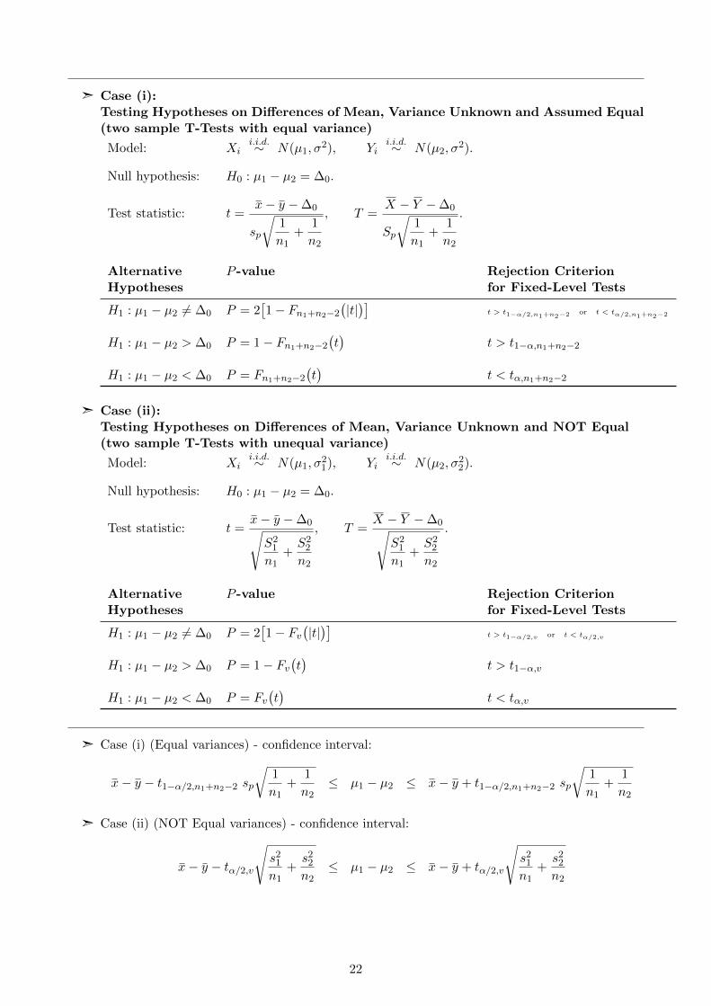
ã Case (i):Testing Hypotheses on Differences of Mean, Variance Unknown and Assumed Equal(two sample T-Tests with equal variance)

Model: Xii.i.d.∼ N(µ1, σ

2), Yii.i.d.∼ N(µ2, σ

2).

Null hypothesis: H0 : µ1 − µ2 = ∆0.

Test statistic: t =x− y −∆0

sp

√1

n1+

1

n2

, T =X − Y −∆0

Sp

√1

n1+

1

n2

.

Alternative P -value Rejection CriterionHypotheses for Fixed-Level Tests

H1 : µ1 − µ2 6= ∆0 P = 2[1− Fn1+n2−2

(|t|)]

t > t1−α/2,n1+n2−2 or t < tα/2,n1+n2−2

H1 : µ1 − µ2 > ∆0 P = 1− Fn1+n2−2(t)

t > t1−α,n1+n2−2

H1 : µ1 − µ2 < ∆0 P = Fn1+n2−2(t)

t < tα,n1+n2−2

ã Case (ii):Testing Hypotheses on Differences of Mean, Variance Unknown and NOT Equal(two sample T-Tests with unequal variance)

Model: Xii.i.d.∼ N(µ1, σ

21), Yi

i.i.d.∼ N(µ2, σ22).

Null hypothesis: H0 : µ1 − µ2 = ∆0.

Test statistic: t =x− y −∆0√S21

n1+S22

n2

, T =X − Y −∆0√

S21

n1+S22

n2

.

Alternative P -value Rejection CriterionHypotheses for Fixed-Level Tests

H1 : µ1 − µ2 6= ∆0 P = 2[1− Fv

(|t|)]

t > t1−α/2,v or t < tα/2,v

H1 : µ1 − µ2 > ∆0 P = 1− Fv(t)

t > t1−α,v

H1 : µ1 − µ2 < ∆0 P = Fv(t)

t < tα,v

ã Case (i) (Equal variances) - confidence interval:

x− y − t1−α/2,n1+n2−2 sp

√1

n1+

1

n2≤ µ1 − µ2 ≤ x− y + t1−α/2,n1+n2−2 sp

√1

n1+

1

n2

ã Case (ii) (NOT Equal variances) - confidence interval:

x− y − tα/2,v

√s21n1

+s22n2

≤ µ1 − µ2 ≤ x− y + tα/2,v

√s21n1

+s22n2

22

9 Linear Regression

ã The collection of statistical tools that are used to model and explore relationships betweenvariables that are related in a nondeterministic manner is called regression analysis. Of keyimportance is the conditional expectation,

E(Y | x) = µY | x = β0 + β1x with Y = β0 + β1x+ ε,

where x is not random and ε is a Normal random variable with E(ε) = 0 and V (ε) = σ2.

ã Simple Linear Regression is the case where both x and y are scalars, in which case the datais,

(x1, y1), . . . , (xn, yn).

Then given estimates of β0 and β1 denoted by β0 and β1 we have

yi = β0 + β1xi + ei i = 1, 2, . . . , n,

where ei, are the residuals and we can also define the predicted observation,

yi = β0 + β1xi.

Ideally it would hold that yi = yi (ei = 0) and thus total mean squared error

L := SSE =

n∑i=1

e2i =

n∑i=1

(yi − yi)2 =

n∑i=1

(yi − β0 − β1xi)2,

would be zero. But in practice, unless σ2 = 0 (and all points lie on the same line), we have thatL > 0.

ã The standard (classic) way of determining the statistics (β0, β1) is by minimisation of L. Thesolution, called the least squares estimators must satisfy

∂L

∂β0

∣∣∣β0β1

= −2n∑i=1

(yi − β0 − β1xi) = 0

∂L

∂β1

∣∣∣β0β1

= −2

n∑i=1

(yi − β0 − β1xi)xi = 0

Simplifying these two equations yields

nβ0 + β1

n∑i=1

xi =n∑i=1

yi

β0

n∑i=1

xi + β1

n∑i=1

x2i =n∑i=1

yixi

These are called the least squares normal equations. The solution to the normal equationsresults in the least squares estimators β0 and β1. Using the sample means, x and y theestimators are,

β0 = y − β1x, β1 =

n∑i=1

yixi −

(n∑i=1

yi

)(n∑i=1

xi

)n

n∑i=1

x2i −

(n∑i=1

xi

)2

n

.

23

ã The following quantities are also of common use:

Sxx =n∑i=1

(xi − x)2 =n∑i=1

x2i −

(n∑i=1

xi

)2

n

Sxy =n∑i=1

(yi − y)(xi − x) =n∑i=1

xiyi −

(n∑i=1

xi)(

n∑i=1

yi)

n

Hence,

β1 =SxySxx

.

Further,

SST =

n∑i=1

(yi − y)2, SSR =

n∑i=1

(yi − y)2, SSE =

n∑i=1

(yi − yi)2.

ã The Analysis of Variance Identity is

n∑i=1

(yi − y

)2=

n∑i=1

(yi − y

)2+

n∑i=1

(yi − yi

)2or,

SST = SSR + SSE .

Also, SSR = β1Sxy.

ã An Estimator of the Variance, σ2 is

σ2 := MSE =SSEn− 2

ã A widely used measure for a regression model is the following ratio of sum of squares, which isoften used to judge the adequacy of a regression model:

R2 =SSRSST

= 1− SSESST

.

E(β0

)= β0, V

(β0

)= σ2

[1

n+

x2

SXX

]

E(β1

)= β1, V

(β1

)=

σ2

SXX.

ã In simple linear regression, the estimated standard error of the slope and the estimatedstandard error of the intercept are

se(β1

)=

√σ2

SXXand se

(β0

)=

√√√√σ2

[1

n+

x2

SXX

]

24

ã The Test Statistic for the Slope is

T =β1 − β1,0√σ2/SXX

H0 : β1 = β1,0 H1 : β1 6= β1,0

Under H0 the test statistic T follows a t - distribution with “n− 2 degree of freedom”.

ã An alternative is to use the F statistic as is common in ANOVA (Analysis of Variance) – notcovered fully in the course.

F =SSR/1

SSE/(n− 2)=MSRMSE

.

Under H0 the test statistic F follows an F - distribution with “1 degree of freedom in thenumerator and n− 2 degrees of freedom in the denominator”.

Analysis of Variance Table for Testing Significance of Regression

Source of Sum of Degrees of Mean F0

Variation Squares Freedom Square

Regression SSR = β1Sxy 1 MSR MSR/MSEError SSE = SST − β1Sxy n− 2 MSETotal SST n− 1

ã There are also confidence intervals for β0 and β1 as well as prediction intervals for observations.We don’t cover these formulas.

ã To check the regression model assumptions we plot the residuals ei and check for (i) Normality.(ii) Constant variance. (iii) Independence.

Logistic Regression:

ã Take the response variable, Yi as a Bernoulli random variable. In this case notice that E(Y ) =P (Y = 1).

ã The logit response function has the form

E(Y)

=exp(β0 + β1x)

1 + exp(β0 + β1x

) .ã Fitting a logistic regression model to data yields estimates of β0 and β1.

ã The following formula is called the odds

E(Y)

1− E(Y) = exp

(β0 + β1x

).

25

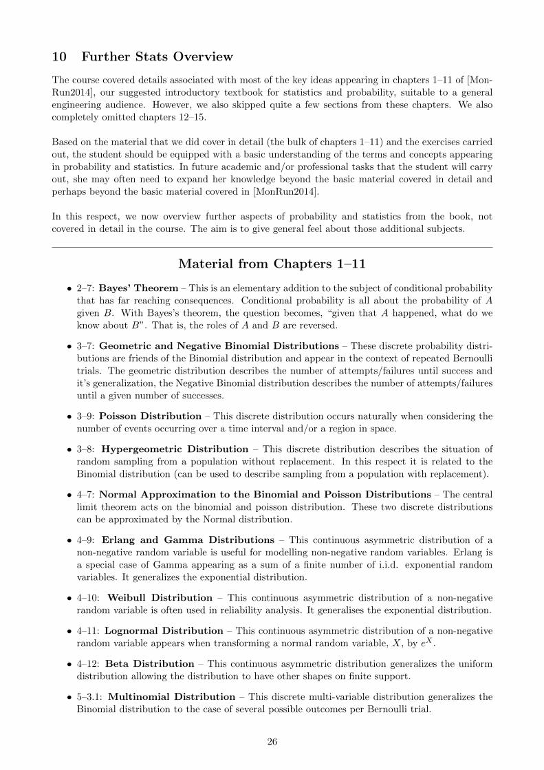
10 Further Stats Overview

The course covered details associated with most of the key ideas appearing in chapters 1–11 of [Mon-Run2014], our suggested introductory textbook for statistics and probability, suitable to a generalengineering audience. However, we also skipped quite a few sections from these chapters. We alsocompletely omitted chapters 12–15.

Based on the material that we did cover in detail (the bulk of chapters 1–11) and the exercises carriedout, the student should be equipped with a basic understanding of the terms and concepts appearingin probability and statistics. In future academic and/or professional tasks that the student will carryout, she may often need to expand her knowledge beyond the basic material covered in detail andperhaps beyond the basic material covered in [MonRun2014].

In this respect, we now overview further aspects of probability and statistics from the book, notcovered in detail in the course. The aim is to give general feel about those additional subjects.

Material from Chapters 1–11

• 2–7: Bayes’ Theorem – This is an elementary addition to the subject of conditional probabilitythat has far reaching consequences. Conditional probability is all about the probability of Agiven B. With Bayes’s theorem, the question becomes, “given that A happened, what do weknow about B”. That is, the roles of A and B are reversed.

• 3–7: Geometric and Negative Binomial Distributions – These discrete probability distri-butions are friends of the Binomial distribution and appear in the context of repeated Bernoullitrials. The geometric distribution describes the number of attempts/failures until success andit’s generalization, the Negative Binomial distribution describes the number of attempts/failuresuntil a given number of successes.

• 3–9: Poisson Distribution – This discrete distribution occurs naturally when considering thenumber of events occurring over a time interval and/or a region in space.

• 3–8: Hypergeometric Distribution – This discrete distribution describes the situation ofrandom sampling from a population without replacement. In this respect it is related to theBinomial distribution (can be used to describe sampling from a population with replacement).

• 4–7: Normal Approximation to the Binomial and Poisson Distributions – The centrallimit theorem acts on the binomial and poisson distribution. These two discrete distributionscan be approximated by the Normal distribution.

• 4–9: Erlang and Gamma Distributions – This continuous asymmetric distribution of anon-negative random variable is useful for modelling non-negative random variables. Erlang isa special case of Gamma appearing as a sum of a finite number of i.i.d. exponential randomvariables. It generalizes the exponential distribution.

• 4–10: Weibull Distribution – This continuous asymmetric distribution of a non-negativerandom variable is often used in reliability analysis. It generalises the exponential distribution.

• 4–11: Lognormal Distribution – This continuous asymmetric distribution of a non-negativerandom variable appears when transforming a normal random variable, X, by eX .

• 4–12: Beta Distribution – This continuous asymmetric distribution generalizes the uniformdistribution allowing the distribution to have other shapes on finite support.

• 5–3.1: Multinomial Distribution – This discrete multi-variable distribution generalizes theBinomial distribution to the case of several possible outcomes per Bernoulli trial.

26

• 5–6: Moment-Generating Functions – A moment generating function is another analyticalway to view the distribution of a random variable (in addition to the CDF, PDF/PMF).

• 7–3.1: Unbiased Estimators – An estimator is unbiased if in expectation it gets the correctvalue. The study of this subject explains the n − 1 in the denominator of the sample variance(as opposed to having the more intuitive value n).

• 7–3: Other general concepts of point estimation – Point estimation is a key area ofstatistics and is studied much further in mathematical statistics courses. There are more waysto quantify and understand the behaviour of an estimator.

• 7–4.1: Method of moments for point estimation – This method of point estimation worksby solving equations specified by moment estimators in the data.

• 7–4.2: Method of maximum likelihood for point estimation – This general method ofpoint estimation has much theory associated with it. It is used in Logistic regression in thecourse. It is a central part of the study of Mathematical statistics.

• 7–4.3: Bayesian Estimation of Parameters – Bayesian statistics is a large branch of statisticswhich allows to incorporate prior beliefs and knowledge in the estimation process. This is oftendone by employing a prior distribution on the unknown parameter and then after carrying outinference obtaining a posterior distribution of the unknown parameter. In Bayesian statistics,as opposed to classic frequentist statistics (taught in most of this course), the parameter is alwaysconsidered a random variable.

• 8–4: Large Sample Confidence Intervals for a Population Proportion – This is aboutestimating a population proportion. For e.g. “proportion of people who support a given can-didate”. In case of large samples, confidence intervals for the population proportion can beobtained using the Normal approximation to the Binomial distribution.

• 8–6: Bootstrap Confidence Interval – A general way of creating approximate confidenceintervals based on Monte Carlo simulation sampling of the estimators.

• 9–4: Tests on the Variance and Standard Deviation of a Normal Distribution –Methods to check hypothesis about variance parameters of a population. These methods usethe Chi-squared (χ2) distribution.

• 9–5: Tests on a Population Proportion – Methods to make hypothesis about a populationproportion as the unknown parameter.

• 9–7: Testing for Goodness of Fit – Methods for checking if a postulated distribution agreeswith the empirical distribution. Here one common method uses the fact that sums of squareddeviations of expected and observed proportions are approximately χ2 distributed.

• 9–8: Contingency Table Tests – A suite of methods that check if different categorial quantitiesare independent or not. Here again, the χ2 distribution is used.

• 9–9: Nonparametric Procedures – Nonparametric statistics is a large branch of statisticswhere there is no assumed family of distributions in the model. One method already studiedin Unit 5 is the Kernel Density Estimation. Some more classic nonparametric methodsthat can be used as alternatives to the T-test and Z-test are the signed rank test. A plus ofthis method is that it does not assume any specific distribution. A drawback comes with lessstatistical power.

• 10–3: Wilcoxon Rank-Sum Nonparametric test for the difference of two means – Thisis a another classic nonparametric method that can replace Z-tests and T-tests.

27

• 10–4: The paired t-test – This test comes together with an experimental design techniquesthat builds on the idea of coupling observations from two treatment (two populations) togetherso as to reduce variability. For example if doing road testing for wear-and-tear of tires, itmeans putting on the same car tires of one type on the left side and another type on the rightside. This then potentially reduces the variability in differences of wear-and-tear between cars,because variability due to driver/car attributes are cancelled. Mathematically the calculationsare identical to a single sample t-test, but conceptually the paired t-test is different. It is animportant thing to know for basic experimental design.

• 10–5: Inferences on the variances of two Normal distributions – This is a suite ofhypothesis tests (and confidence intervals) asking if two populations have the same variance ornot. From a model-selection perspective, using these tests can be sometimes useful for choosinga specific model for comparing population means (as covered in the two sample inference, Unit8).

• 10–6: Inferences on two population proportions – This is a suite of hypothesis tests (andconfidence intervals) comparing population proportions in two populations.

• 11–9: Regression on Transformed Variables – Linear regression on the original variables isoften not a sensible assumption. E.g. when there exists a logarithmic or quadratic relationship.By transforming variables, linear regression may sometimes be applied to other models. Anotherreason for (sometimes) transforming variables is to match the data to the model assumptions(constant variance and Normal residuals).

Material from Further Chapters

• Chapter 12 – Multiple Linear Regression – Linear regression goes well beyond finding therelationship of Y on (the scalar) X. In many practical situations, X is taken as a vector and therelationship of different components of this vector of Y are of interest. Multiple linear regressionis then used.

• Chapter 13 – Design and Analysis of Single-Factor Experiments: The Analysis ofVariance – The Analysis of Variance (ANOVA) is a very common method for comparing meansof two or more populations under the assumption that variances are equal. It is key to knowthat this is a method for comparing means, even though the name is variance. The variabilitybetween sample means and within sample means is used to test the hypothesis that means aredifferent, or the same. Under the null-hypothesis, stating all means are equal, the test statisticfollows the well known F -distribution. ANOVA is often taught as part of a basic statisticscourse and is a very common method in practice. Understanding ANOVA, constitutes the basicunderstanding leading towards design of experiments. Note the the case of two samples, wascovered in Unit 8 of the course (two sample inference). In that case, the T-test described isclosely related to ANOVA.

• Chapter 14 – Design of Experiments with Several Factors – This is a more advanced aspectof scientific statistics. Often there are several factors that are postulated and trying out all pos-sible combinations is difficult. This branch of design of experiments suggests sampling methodsthat allow to efficiently (from a statistical perspective) determine the validity of hypothesis. Oneaspect here is two-way ANOVA and other more advanced aspects include factorial designs ofexperiments.

• Chapter 15 – Statistical Quality Control – This branch of industrial statistics is often usedin manufacturing/mining industries. The essence is to observe a time-series of statistics such asmeans, variances and ranges. A key goal is to have criteria for indicating where the “processis out of control” - indicating that some change has happened in the system and it should befurther investigated.

28