stat 830 generating...

STAT 830Generating Functions

Richard Lockhart

Simon Fraser University

STAT 830 — Fall 2011

Richard Lockhart (Simon Fraser University) STAT 830 Generating Functions STAT 830 — Fall 2011 1 / 21

What I think you already have seen

Definition of Moment Generating Function

Basics of complex numbers


What I want you to learn

Definition of cumulants and cumulant generating function.

Definition of Characteristic Function

Elementary features of complex numbers

How they “characterize” a distribution

Relation to sums of independent rvs


Moment Generating Functions pp 56-58

Def’n: The moment generating function of a real valued X is

MX (t) = E (etX )

defined for those real t for which the expected value is finite.

Def’n: The moment generating function of X ∈ Rp is

MX (u) = E [eutX ]

defined for those vectors u for which the expected value is finite.

Formal connection to moments:

MX (t) =∞∑

k=0

E [(tX )k ]/k!

=∞∑

k=0

µ′

ktk/k! .

Sometimes can find power series expansion of MX and read off themoments of X from the coefficients of tk/k!.


Moments and MGFs

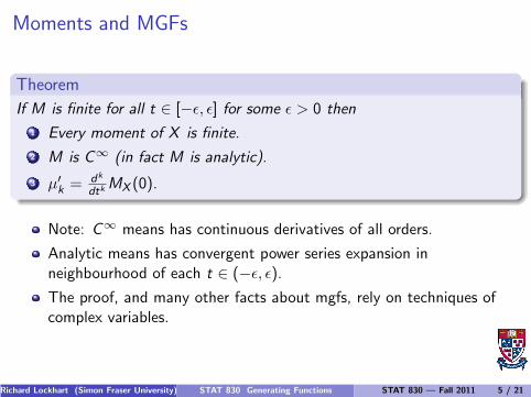
Theorem

If M is finite for all t ∈ [−ǫ, ǫ] for some ǫ > 0 then

1 Every moment of X is finite.

2 M is C∞ (in fact M is analytic).

3 µ′

k = dk

dtkMX (0).

Note: C∞ means has continuous derivatives of all orders.

Analytic means has convergent power series expansion inneighbourhood of each t ∈ (−ǫ, ǫ).

The proof, and many other facts about mgfs, rely on techniques ofcomplex variables.


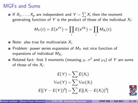
MGFs and Sums

If X1, . . . ,Xp are independent and Y =∑

Xi then the momentgenerating function of Y is the product of those of the individual Xi :

MY (t) = E (etY ) =∏

i

E (etXi ) =∏

i

MXi(t).

Note: also true for multivariate Xi .

Problem: power series expansion of MY not nice function ofexpansions of individual MXi

.

Related fact: first 3 moments (meaning µ, σ2 and µ3) of Y are sumsof those of the Xi :

E (Y ) =∑

E (Xi )

Var(Y ) =∑

Var(Xi )

E [(Y − E (Y ))3] =∑

E [(Xi − E (Xi ))3]


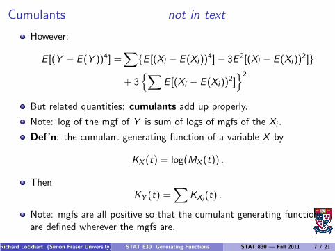
Cumulants not in text

However:

E [(Y − E (Y ))4] =∑

{E [(Xi − E (Xi ))4]− 3E 2[(Xi − E (Xi ))

2]}

+ 3{

∑

E [(Xi − E (Xi ))2]}2

But related quantities: cumulants add up properly.

Note: log of the mgf of Y is sum of logs of mgfs of the Xi .

Def’n: the cumulant generating function of a variable X by

KX (t) = log(MX (t)) .

ThenKY (t) =

∑

KXi(t) .

Note: mgfs are all positive so that the cumulant generating functionsare defined wherever the mgfs are.


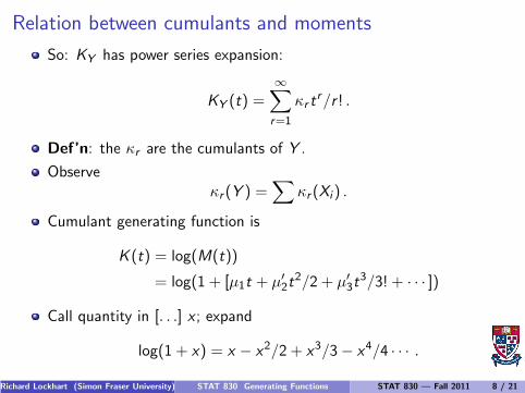
Relation between cumulants and moments

So: KY has power series expansion:

KY (t) =∞∑

r=1

κr tr/r ! .

Def’n: the κr are the cumulants of Y .

Observeκr (Y ) =

∑

κr (Xi ) .

Cumulant generating function is

K (t) = log(M(t))

= log(1 + [µ1t + µ′

2t2/2 + µ′

3t3/3! + · · · ])

Call quantity in [. . .] x ; expand

log(1 + x) = x − x2/2 + x3/3− x4/4 · · · .


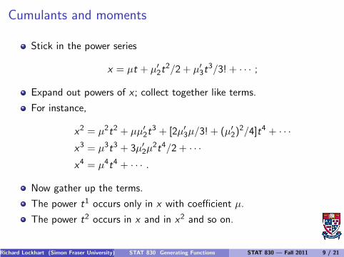
Cumulants and moments

Stick in the power series

x = µt + µ′

2t2/2 + µ′

3t3/3! + · · · ;

Expand out powers of x ; collect together like terms.

For instance,

x2 = µ2t2 + µµ′

2t3 + [2µ′

3µ/3! + (µ′

2)2/4]t4 + · · ·

x3 = µ3t3 + 3µ′

2µ2t4/2 + · · ·

x4 = µ4t4 + · · · .

Now gather up the terms.

The power t1 occurs only in x with coefficient µ.

The power t2 occurs in x and in x2 and so on.


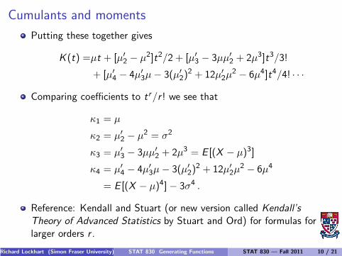
Cumulants and moments

Putting these together gives

K (t) =µt + [µ′

2 − µ2]t2/2 + [µ′

3 − 3µµ′

2 + 2µ3]t3/3!

+ [µ′

4 − 4µ′

3µ− 3(µ′

2)2 + 12µ′

2µ2 − 6µ4]t4/4! · · ·

Comparing coefficients to tr/r ! we see that

κ1 = µ

κ2 = µ′

2 − µ2 = σ2

κ3 = µ′

3 − 3µµ′

2 + 2µ3 = E [(X − µ)3]

κ4 = µ′

4 − 4µ′

3µ− 3(µ′

2)2 + 12µ′

2µ2 − 6µ4

= E [(X − µ)4]− 3σ4 .

Reference: Kendall and Stuart (or new version called Kendall’sTheory of Advanced Statistics by Stuart and Ord) for formulas forlarger orders r .


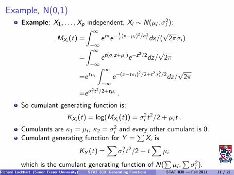
Example, N(0,1)Example: X1, . . . ,Xp independent, Xi ∼ N(µi , σ

2i ):

MXi(t) =

∫

∞

−∞

etxe−12(x−µi )

2/σ2i dx/(

√2πσi )

=

∫

∞

−∞

et(σiz+µi )e−z2/2dz/√2π

=etµi

∫

∞

−∞

e−(z−tσi )2/2+t2σ2

i /2dz/√2π

=eσ2i t

2/2+tµi .

So cumulant generating function is:

KXi(t) = log(MXi

(t)) = σ2i t

2/2 + µi t .

Cumulants are κ1 = µi , κ2 = σ2i and every other cumulant is 0.

Cumulant generating function for Y =∑

Xi is

KY (t) =∑

σ2i t

2/2 + t∑

µi

which is the cumulant generating function of N(∑

µi ,∑

σ2i ).


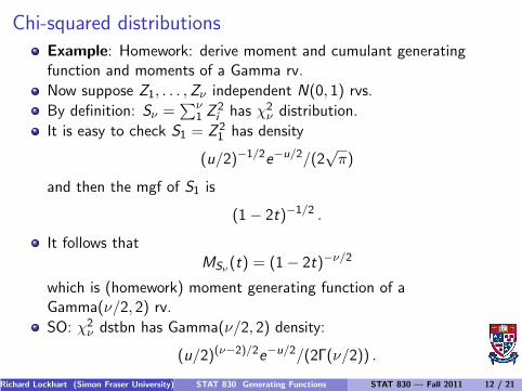
Chi-squared distributions

Example: Homework: derive moment and cumulant generatingfunction and moments of a Gamma rv.

Now suppose Z1, . . . ,Zν independent N(0, 1) rvs.

By definition: Sν =∑ν

1 Z2i has χ2

ν distribution.

It is easy to check S1 = Z 21 has density

(u/2)−1/2e−u/2/(2√π)

and then the mgf of S1 is

(1− 2t)−1/2 .

It follows thatMSν (t) = (1− 2t)−ν/2

which is (homework) moment generating function of aGamma(ν/2, 2) rv.

SO: χ2ν dstbn has Gamma(ν/2, 2) density:

(u/2)(ν−2)/2e−u/2/(2Γ(ν/2)) .


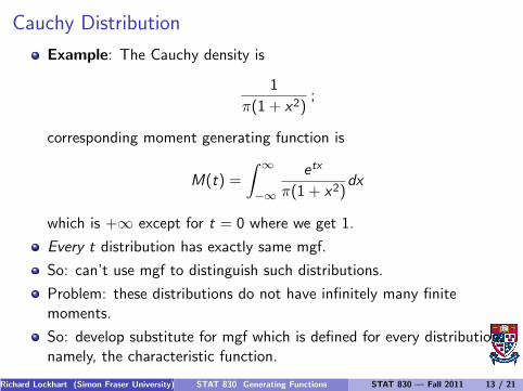
Cauchy Distribution

Example: The Cauchy density is

1

π(1 + x2);

corresponding moment generating function is

M(t) =

∫

∞

−∞

etx

π(1 + x2)dx

which is +∞ except for t = 0 where we get 1.

Every t distribution has exactly same mgf.

So: can’t use mgf to distinguish such distributions.

Problem: these distributions do not have infinitely many finitemoments.

So: develop substitute for mgf which is defined for every distribution,namely, the characteristic function.


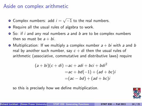
Aside on complex arithmetic

Complex numbers: add i =√−1 to the real numbers.

Require all the usual rules of algebra to work.

So: if i and any real numbers a and b are to be complex numbersthen so must be a+ bi .

Multiplication: If we multiply a complex number a+ bi with a and breal by another such number, say c + di then the usual rules ofarithmetic (associative, commutative and distributive laws) require

(a + bi)(c + di) =ac + adi + bci + bdi2

=ac + bd(−1) + (ad + bc)i

=(ac − bd) + (ad + bc)i

so this is precisely how we define multiplication.


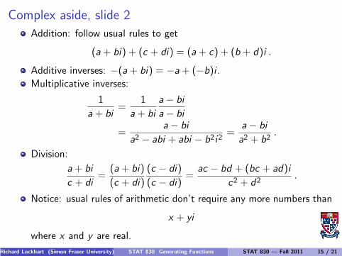
Complex aside, slide 2

Addition: follow usual rules to get

(a+ bi) + (c + di) = (a+ c) + (b + d)i .

Additive inverses: −(a+ bi) = −a+ (−b)i .

Multiplicative inverses:

1

a+ bi=

1

a+ bi

a− bi

a− bi

=a− bi

a2 − abi + abi − b2i2=

a− bi

a2 + b2.

Division:

a+ bi

c + di=

(a+ bi)

(c + di)

(c − di)

(c − di)=

ac − bd + (bc + ad)i

c2 + d2.

Notice: usual rules of arithmetic don’t require any more numbers than

x + yi

where x and y are real.


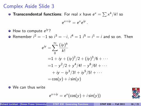
Complex Aside Slide 3

Transcendental functions: For real x have ex =∑

xk/k! so

ex+iy = exe iy .

How to compute e iy?

Remember i2 = −1 so i3 = −i , i4 = 1 i5 = i1 = i and so on. Then

e iy =∞∑

0

(iy)k

k!

=1 + iy + (iy)2/2 + (iy)3/6 + · · ·=1− y2/2 + y4/4!− y6/6! + · · ·+ iy − iy3/3! + iy5/5! + · · ·

=cos(y) + i sin(y)

We can thus write

ex+iy = ex(cos(y) + i sin(y))


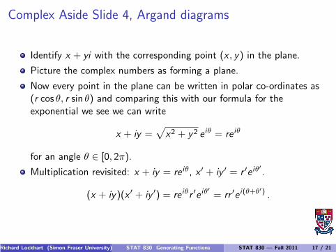
Complex Aside Slide 4, Argand diagrams

Identify x + yi with the corresponding point (x , y) in the plane.

Picture the complex numbers as forming a plane.

Now every point in the plane can be written in polar co-ordinates as(r cos θ, r sin θ) and comparing this with our formula for theexponential we see we can write

x + iy =√

x2 + y2 e iθ = re iθ

for an angle θ ∈ [0, 2π).

Multiplication revisited: x + iy = re iθ, x ′ + iy ′ = r ′e iθ′

.

(x + iy)(x ′ + iy ′) = re iθr ′e iθ′

= rr ′e i(θ+θ′) .


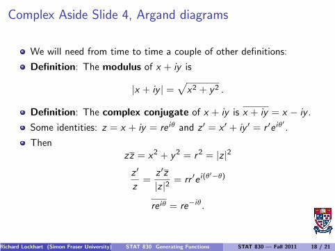
Complex Aside Slide 4, Argand diagrams

We will need from time to time a couple of other definitions:

Definition: The modulus of x + iy is

|x + iy | =√

x2 + y2 .

Definition: The complex conjugate of x + iy is x + iy = x − iy .

Some identities: z = x + iy = re iθ and z ′ = x ′ + iy ′ = r ′e iθ′

.

Thenzz = x2 + y2 = r2 = |z |2

z ′

z=

z ′z

|z |2 = rr ′e i(θ′−θ)

re iθ = re−iθ.


Notes on calculus with complex variables

Essentially usual rules apply so, for example,

d

dte it = ie it .

We will (mostly) be doing only integrals over the real line; the theoryof integrals along paths in the complex plane is a very important partof mathematics, however.

FACT: (not used explicitly in course). If f : C 7→ C is differentiablethen f is analytic (has power series expansion).

End of Aside


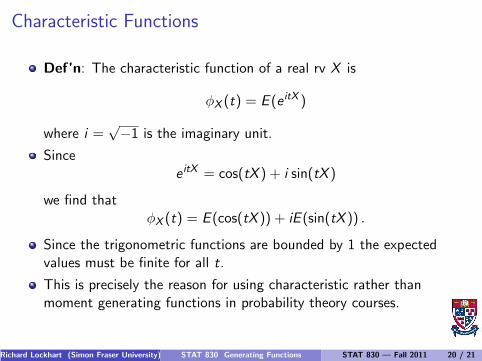
Characteristic Functions

Def’n: The characteristic function of a real rv X is

φX (t) = E (e itX )

where i =√−1 is the imaginary unit.

Sincee itX = cos(tX ) + i sin(tX )

we find thatφX (t) = E (cos(tX )) + iE (sin(tX )) .

Since the trigonometric functions are bounded by 1 the expectedvalues must be finite for all t.

This is precisely the reason for using characteristic rather thanmoment generating functions in probability theory courses.


Role of transforms in characterization cf Th 3.33, p 57

Theorem

For any two real rvs X and Y the following are equivalent:

1 X and Y have the same distribution, that is, for any (Borel) set A wehave

P(X ∈ A) = P(Y ∈ A) .

2 FX (t) = FY (t) for all t.

3 φX (t) = E (e itX ) = E (e itY ) = φY (t) for all real t.

Moreover, all these are implied if there is ǫ > 0 such that for all |t| ≤ ǫ

MX (t) = MY (t) < ∞ .


stat 830 generating...

Documents