Stat 579: Generalized Linear Models andExtensions

Linear Mixed Models for Longitudinal Data

Yan LuApril, 2018, week 12

1 / 34

Correlated data

I multivariate observations

I clustered data

I repeated measurement

I longitudinal data

I spatially correlated data

2 / 34

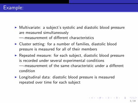
Example:

I Multivariate: a subject’s systolic and diastolic blood pressureare measured simultaneously—-measurement of different characteristics

I Cluster setting: for a number of families, diastolic bloodpressure is measured for all of their members

I Repeated measure: for each subject, diastolic blood pressureis recorded under several experimental conditions—-measurement of the same characteristic under a differentcondition

I Longitudinal data: diastolic blood pressure is measuredrepeated over time for each subject

3 / 34

Problems of repeated measure and longitudinal design:

I Order effectExample: in evaluating five different advertisements, subjectsmay tend to give higher (or lower) ratings for advertisementsshown-toward the end of the sequence than at the beginningRemedy: randomization of the treatment orders

I Carry over effectExample: in evaluating five different soup recipes, a blandrecipe may get a higher (or lower) rating when preceded by ahighly spiced recipe than when preceded by a blander recipe.Remedy: allowing sufficient time between treatments.Example: in evaluating a new drug, it is often noticed thatthe effect of the drug began to wear off over time.Remedy: consider a mixed model by incorporating time effecttypical models: Random intercepts model, and Random slopesand intercepts model

4 / 34

Example: Childhood obesity

n children are followed longitudinally (over time)

I body mass index (BMI = WT/HT2) has been recorded ateach time (age)

I interested in the relationship of BMI as a function of age

I data structure:

time (age) 1 time (age) 2 · · · time (age) ni1st child y11 y12 y1n12nd child y21 y22 y2n2

...nth child yn1 yn2 ynnn

5 / 34

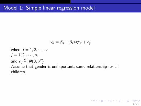
Model 1: Simple linear regression model

yij = β0 + β1ageij + εij

where i = 1, 2. · · · , n,j = 1, 2, · · · , niand εij

iid∼ N(0, σ2)Assume that gender is unimportant, same relationship for allchildren.

6 / 34

Model 2: Intercepts and slopes vary by child

yij = β0i + β1iageij + εij

where i = 1, 2. · · · , n,j = 1, 2, · · · , niand εij

iid∼ N(0, σ2)

I Model 1: 2 parameters (β0, β1)

I Model 2: 2n parameters (β0i , β1i )

I Responses on the same child are likely to be correlated, iidassumption may not work

7 / 34

Model 3: Mixed model

Treat the subject specific intercepts β0i and slopes β1i as r.vs

I β0i = β0 + β∗0i , β∗0i

iid∼ N(0, σ20)

I β1i = β1 + β∗1i , β∗1i

iid∼ N(0, σ21)

I β∗0i , β∗1i measure the difference between the population mean

intercept and slope (β0, β1) and the subject specific interceptand slope (β0i , β1i )

yij = β0 + β∗0i + (β1 + β∗1i )ageij + εij

= β0 + β1ageij + β∗0i + β∗1iageij + εij

I β0 + β1ageij : population average regression line

I β∗0i + β∗1iageij : subject specific deviation from populationaverage

I A special case of a linear mixed model (LMM): fixed effects(β0, β1) + random effects (β∗0i , β

∗1i )

8 / 34

Advantages:

I responses on the same individual are correlatedyi1, yi2, · · · , yini all depend on β0i , β1i

I Model 2: 2n parametersModel 3: 5 parameters

I Model 2 only applies to the individuals selected from study,while Model 3, individuals are sampled as representatives of anunderlying population, therefore, applying to the population

9 / 34

General Linear Models for Longitudinal Data

yi =

yi1yi2...

yini

,µi =

µi1µi2

...µini

, εi =

εi1εi2...εini

yi s are responses at times ti1, ti2 · · · , tini

yi = µi + εi

I number of time points can vary by individual

I assume that µi = Xi ni×pβp×1, Xi may be individual specific

I assume E (εi ) = 0,Var(εi ) = Var(yi ) = Σi

I often assume εi ∼ Nni (0,Σi ) or equivalently, yi ∼ Nni (µi ,Σi )

10 / 34

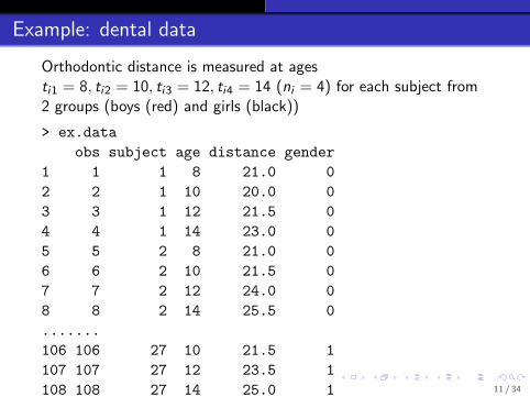
Example: dental data

Orthodontic distance is measured at agesti1 = 8, ti2 = 10, ti3 = 12, ti4 = 14 (ni = 4) for each subject from2 groups (boys (red) and girls (black))

> ex.data

obs subject age distance gender

1 1 1 8 21.0 0

2 2 1 10 20.0 0

3 3 1 12 21.5 0

4 4 1 14 23.0 0

5 5 2 8 21.0 0

6 6 2 10 21.5 0

7 7 2 12 24.0 0

8 8 2 14 25.5 0

.......

106 106 27 10 21.5 1

107 107 27 12 23.5 1

108 108 27 14 25.0 1 11 / 34

> aa<-aggregate(distance~age+gender, data=ex.data, mean)

#cell means

> aa

age gender distance

1 8 0 21.18182

2 10 0 22.22727

3 12 0 23.09091

4 14 0 24.09091

5 8 1 22.87500

6 10 1 23.81250

7 12 1 25.71875

8 14 1 27.46875

12 / 34

Figure 1: Sample means at each time across children

2122

2324

2526

27

age

distan

ce

8 10 12 14

gender

1

0

Increasing linear trend with time, males (red) and females (black)have different intercepts and possibly different slopes.

13 / 34

Starting model

yij = µij + εij

i : subject, j : timeLet

δi =

{1 if boy0 if girl

Letµij = β0 + β1δi + β2tj + β3(δi tj)

δi : indicator effect for gendertj : linear time effect(δi tj): time and gender interactions

14 / 34

µij = β0 + β1δi + β2tj + β3(δi tj)

For δi = 0 (girls)

µij = β0 + β1(0) + β2tj + β3(0) = β0 + β2tj

For δi = 1 (boys)

µij = β0 + β1(1) + β2tj + β3(1 ∗ tj) = (β0 + β1) + (β2 + β3)tj

gender intercept slope

girls β0 β2boys β0 + β1 β2 + β3

15 / 34

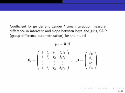
Coefficient for gender and gender * time interaction measuredifference in intercept and slope between boys and girls, GDP(group difference parametrization) for the model

µi = Xiβ

Xi =

1 δi t1 δi t11 δi t2 δi t2...

......

...1 δi tn δi tn

, β =

β0β1β2β3

16 / 34

Separate group parametrization

An equivalent model is to specify

µij = β0(1− δi ) + β1δi + β2(1− δi )tj + β3(δi tj)

For δi = 0 (girls), µij = β0 +β2tj For δi = 1 (boys), µij = β1 +β3tj

µi = Xiβ

Separate group parametrization (SGP) µi1...µini

=

1− δi δi (1− δi )tj δi tj...

......

...1− δi δi (1− δi )tj δi tj

β0β1β2β3

17 / 34

For girls

Xi =

1 0 t1 01 0 t2 0...

......

...1 0 tni 0

For boys

Xi =

0 1 0 t10 1 0 t2...

......

...0 1 0 tni

18 / 34

Split Plot model

Alternatively, we could consider the split-plot model

µij = µ+ τi + δj + (τδ)ij

The models relates the mean to a linear function of time wouldappear to be more appealing.

19 / 34

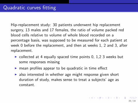
Quadratic curves fitting

Hip-replacement study: 30 patients underwent hip replacementsurgery, 13 males and 17 females, the ratio of volume packed redblood cells relative to volume of whole blood recorded on apercentage basis, was supposed to be measured for each patient atweek 0 before the replacement, and then at weeks 1, 2 and 3, afterreplacement.

I collected at 4 equally spaced time points 0, 1,2 3 weeks butsome responses missing

I mean profiles appear to be quadratic in time effect

I also interested in whether age might response given shortduration of study, makes sense to treat a subjects’ age asconstant.

20 / 34

Let

δi =

{1 males0 females

yij = µij + εij

µij = β0 + β1tij + β2t2ij + β3δi + β4δi tij + β5δi t

2ij

For femalesµij = β0 + β1tij + β2t

2ij

For males

µij = (β0 + β3) + (β1 + β4)tij + (β2 + β5)t2ij

quadratic curves shift up or down with age, but amount of shift issame for males and females. We could allow the shift to be sexdependent by includes a gender*age interaction.

21 / 34

Modeling the covariance matrix Σi

yi = µi + εi

Var(εi ) = Var(yi ) = Σi (ni×ni )

For balanced case

I ni = n, t1, t2, · · · , tnI assume no missing data

I further, assume that Σi = Σ

22 / 34

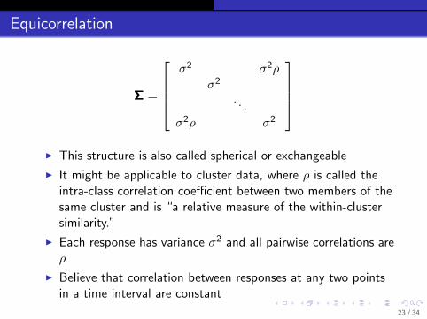
Equicorrelation

Σ =

σ2 σ2ρ

σ2

. . .

σ2ρ σ2

I This structure is also called spherical or exchangeable

I It might be applicable to cluster data, where ρ is called theintra-class correlation coefficient between two members of thesame cluster and is “a relative measure of the within-clustersimilarity.”

I Each response has variance σ2 and all pairwise correlations areρ

I Believe that correlation between responses at any two pointsin a time interval are constant

23 / 34

Compound symmetry

A special case of equicorrelation, arises by enforcingρ = σ2B/(σ2B + σ2e ) for some σ2B and σ2e . In this case,σ2 = σ2B + σ2e , then

Σ =

σ2B + σ2e σ2B σ2B · · · σ2Bσ2B σ2B + σ2e σ2B · · · σ2B...

.... . .

......

σ2B σ2B σ2B · · · σ2B + σ2e

n×n

Recall that a split plot design has this variance structure.

24 / 34

Unstructured–arbitrary variances and covariances

Σ =

σ21 σ12 · · · σ1nσ21 σ22 σ2n

.... . .

...σn1 σn2 · · · σ2n

I the variance-covariance matrix contains, n(n − 1)/2 + n

nuisance parameters to be estimated

I estimation of this structure may only convergence for N >> n

I the statistical power under this structure is reduced since theonly constraint on Σi is that it be symmetric

25 / 34

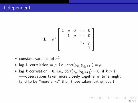
1 dependent

Σ = σ2

1 ρ 0 · · · 0

1 ρ · · · 0. . . ρ

1

I constant variance of σ2

I lag 1, correlation = ρ, i.e., corr(yij , yi(j±1)) = ρ

I lag k correlation =0, i.e., corr(yij , yi(j±k)) = 0, if k > 1—–observations taken more closely together in time mighttend to be “more alike” than those taken further apart

26 / 34

AR(1): auto regressive order 1 (equally spaced in time)

Σ = σ2

1 ρ ρ2 · · · ρn−1

1 ρ · · · ρn−2

. . .. . .

...1 ρ

1

I constant variance σ2

I corr(yij , yi(j±k)) = ρk

27 / 34

Unequally spaced in time

The above models make sense for equally spaced times. Howabout if times are unequally spaced, but we still have same timeseach subject?

I compound symmetry: if you believe that correlations betweenresponses at any two points in a time interval are constant,then ok

I unstructured: ok

I 1 dependent, not for sure, if t3 = t2 + ε with ε small, shouldcorr(yt1 , yt2) = ρ, yet corr(yt1 , yt3) = 0

I AR(1), same issue as 1 dependent

28 / 34

Generalization of AR(1) to unequally spaced times

I Markov model-correlation is a function of distance betweentimes

I Let djh = |tj − th|, then Markov model has—- var(ytj ) = σ2

—- corr(ytj , yth) = ρdjh

29 / 34

Deciding among covariance models

I inspection of sample covariance matrices

I can use formal test in some cases, model selection methodsAIC, BIC, for non-nested models

30 / 34

Unbalanced case: or some observations are missing onsome units

Example: (t1, t2, t3, t4) = (0, 1, 2, 3)For unit i , observation at time t3 is not available ni = 3. Let

yi =

yi1yi2yi4

denote the observations at times (t1, t2, t4)′ = (0, 1, 3)′

Assume that var(yij) = σ2 for all j , we thus want a model for

Σi = var(yi ) =

σ2 cov(yi1, yi2) cov(yi1, yi4)cov(yi2, yi1) σ2 cov(yi2, yi4)cov(yi4, yi1) cov(yi4, yi2) σ2

31 / 34

I Compound symmetry: represented in the same way regardlessof the missing value——observations any distance apart have the same correlation

I Unstructured ,

Σi = var(yi ) =

σ21 σ12 σ14σ21 σ22 σ24σ41 σ42 σ24

I One-dependent, which says that only observations adjacent in

time are correlated, this matrix becomes

Σi = var(yi ) =

σ2 ρσ2 0ρσ2 σ2 0

0 0 σ2

32 / 34

I AR(1):

Σi = var(yi ) = σ2

1 ρ ρ3

ρ 1 ρ2

ρ3 ρ2 1

Comments: if all observations were intended to be taken atthe same times, but some are not available, the covariancematrix must be carefully constructed.

33 / 34

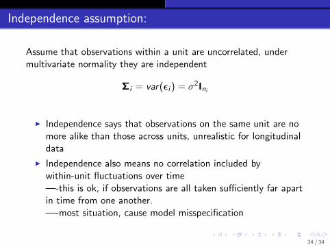
Independence assumption:

Assume that observations within a unit are uncorrelated, undermultivariate normality they are independent

Σi = var(εi ) = σ2Ini

I Independence says that observations on the same unit are nomore alike than those across units, unrealistic for longitudinaldata

I Independence also means no correlation included bywithin-unit fluctuations over time—-this is ok, if observations are all taken sufficiently far apartin time from one another.—-most situation, cause model misspecification

34 / 34