standard operating procedures manual for the … · 1 standard operating procedures manual for the...
TRANSCRIPT
1
STANDARD OPERATING PROCEDURES MANUAL
FOR THE
BREWER SPECTROPHOTOMETER
Version: D.01
June 12, 2008
Environment Canada
4905 Dufferin Street
Toronto, Ontario
Canada M3H 5T4
2
Table of Contents
1. Document History--------------------------------------------------------------------------- 8
2. Acknowledgements ------------------------------------------------------------------------- 9
3. Preface--------------------------------------------------------------------------------------- 10
4. Abbreviations ------------------------------------------------------------------------------ 11
5. Safety Issues-------------------------------------------------------------------------------- 12 5.1. Overview 12 5.2. Material Safety Data Sheets (MSDS) 12 5.3. Hazard—Electrocution 13
5.3.1. Power LEDs ..................................................................................................13
5.3.2. Power Switch Terminals ...............................................................................14
5.3.3. Power Cables ................................................................................................14
5.3.4. Tracker Power Terminal Strip.......................................................................14 5.3.5. Maintenance and Weather.............................................................................14
5.4. Hazard—Permanent Damage to Eyesight from UV Irradiance 14 5.5. Hazard—Back Injury from Handling Brewer Spectrophotometer 14 5.6. Hazard—Injury due to Tripping over Cables or Tripod 15 5.7. Hazard—Information from the Manufacturer 15
6. Introduction-------------------------------------------------------------------------------- 16 6.1. Measurement Principles and Theory 16
6.1.1. Ozone and sulfur dioxide ..............................................................................16
6.1.2. UV.................................................................................................................16
6.1.3. Umkehr .........................................................................................................16 6.1.4. Aerosol optical depth ....................................................................................16
6.1.5. NO2 ...............................................................................................................16 6.2. The Brewer Spectrophotometer 16 6.3. Brewer Models and Measurement Capabilities 17 6.4. Basic Component Assemblies 19 6.5. Communication Configuration 20
7. Maintenance ------------------------------------------------------------------------------- 21 7.1. Critical Maintenance Warnings 21
7.1.1. Overview.......................................................................................................21 7.1.2. Photomultiplier Tube ....................................................................................21
7.1.3. Excess Moisture ............................................................................................21
7.1.4. Optical Surfaces ............................................................................................21
7.1.5. Lubricants......................................................................................................21 7.2. Routine Maintenance 22
7.2.1. Overview.......................................................................................................22
7.2.2. Brewer Log Form..........................................................................................22
7.2.3. Daily Maintenance ........................................................................................23 7.2.4. Bi-Weekly Maintenance (every two weeks) .................................................25
7.2.5. Bi-Monthly (every two months)....................................................................31
7.2.6. Unscheduled Maintenance ............................................................................33
8. Hardware Installation ------------------------------------------------------------------- 37
3
8.1. Overview 37 8.2. Brewer System Requirements 37 8.3. Site Selection 38 8.4. Installation Surface 38
8.4.1. Building Roof Top Installation .....................................................................39
8.4.2. Ground Installation .......................................................................................39
8.4.3. Platform installation on Building Roof Top or on Ground...........................39 8.5. Brewer Spectrophotometer Assembly Instructions 39 8.6. Leveling the Brewer Tripod 40 8.7. Leveling the Brewer’s Optical Assembly 44 8.8. Protective Covers for NO2/Red Brewer Viewers 47 8.9. Computer System Installation and Connection 47
9. Software Installation and Configuration -------------------------------------------- 48 9.1. Overview 48 9.2. Installation of current version of the Brewer GWBasic Software 48 9.3. Computer and Brewer Software Configuration for Autoboot 49 9.4. Start the Brewer Software 49 9.5. Setting the Buffer Delay (if required) 50 9.6. Brewer Time-Keeping Options 50 9.7. Configure Software for Brewer Location and Station Pressure 51 9.8. Configure Software for Date and Time 52 9.9. Sighting 52 9.10. Place the Brewer on Schedule 52
10. Data Acquisition ----------------------------------------------------------------------- 55 10.1. Overview 55 10.2. Scheduled Operation and Writing Schedules 55 10.3. Scheduling Commands 56
10.3.1. Scheduling Measurement Commands.........................................................56
10.3.2. Scheduling Diagnostic Commands .............................................................57 10.4. Writing Schedules 57 10.5. Tips for Schedule Writing 57
10.5.1. Micrometer Movement ...............................................................................57 10.5.2. Lamp Commands ........................................................................................57
10.5.3. DS, ZS, FZ and UV Measurements ............................................................58
10.5.4. Focussed Moon Observations .....................................................................58
10.5.5. Umkehr Commands ....................................................................................58
10.5.6. CI and CZ Scans .........................................................................................58 10.6. Sample Schedules 59
11. Routine Diagnostics ------------------------------------------------------------------- 61 11.1. Overview 61 11.2. Daily Error Checks 61 11.3. Weekly Diagnostic Checks 61
11.3.1. Mercury Lamp Test (hg) .............................................................................62
11.3.2. Standard LampTest (sl)...............................................................................62
11.3.3. A/D Information Checks (ap) .....................................................................63
11.3.4. Dead Time Test (dt) ....................................................................................63
11.3.5. Run Stop Test (rs) .......................................................................................65
4
12. Data Analysis and Archival Procedures ------------------------------------------ 67
13. Data Quality Control and Data Quality Assurance ---------------------------- 68 14. Calibrations ----------------------------------------------------------------------------- 69
14.1. Instrument Calibration for Ozone Measurement Introduction 69 14.2. The Information Collected During a Calibration 69
14.2.1. Instrument Performance History.................................................................69 14.2.2. Data Comparison ........................................................................................70
14.2.3. Optics Mechanical Check (all optical surfaces properly constrained) ........70
14.2.4. Optical Surface Visual Inspection...............................................................70
14.2.5. Alignment check .........................................................................................71
14.2.6. Motor Inspection and Electro-mechanical Testing .....................................71
14.2.7. Azimuth and Elevation Motor Functionality Test ......................................71
14.2.8. Elevation Axis Alignment and Instrument Levelling .................................71 14.2.9. Wavelength Dispersion Constants ..............................................................72
14.2.10. Slit Function..............................................................................................72
14.2.11. Relative Sensitivity (among wavelengths)................................................72
14.2.12. Absolute temperature coefficients ............................................................72
14.2.13. Delay Constant..........................................................................................73
14.2.14. Run/Stop Test Results (test of chopper dynamics) ...................................73
14.2.15. Dead Time.................................................................................................73 14.2.16. Relative Dispersion Constants (grating 2 v. grating 1 in double) .............74
14.2.17. Calibration Step Number (on sun and relative to mercury lamp) .............74
14.2.18. Grating offset(s) (2 in double spectrometer).............................................75
14.2.19. Photomultiplier High Voltage Setting ......................................................75
14.2.20. Calibration of temperature, humidity and pressure sensors. .....................75
14.2.21. Measurement of Temperature Dependence of Absolute Sensitivity.........76
14.2.22. Determination of the neutral density filter properties ...............................76 14.2.23. Sun Scan to Determine Proper Wavelength Setting .................................76
14.2.24. Calculation of Effective Ozone Absorption Coefficients .........................77
14.2.25. Determination of Extraterrestrial Constant ...............................................77 14.3. Post Calibration 77 14.4. Reporting 78 14.5. Sample calibration report as currently provided by IOS to customers. 78
15. List of available commands---------------------------------------------------------- 79 15.1. Overview 79 15.2. AP (ext) Monitor Voltages Printout 79 15.3. AS (int) Azimuth Tracker to the Sun 79 15.4. AU (ext) Automatic Operation 80 15.5. AZ (ext) Azimuth Tracker Zeroing 80 15.6. B0 (int) Turn off Lamps 80 15.7. B1 (int) Mercury Lamp ON 80 15.8. B2 (int) Standard Lamp ON 80 15.9. CF (ext) Instrument Constants File Update 80 15.10. CI (int) Lamp Scan on Slit #1 81 15.11. CO (int) Comments 81 15.12. CY (int) Slitmask Cycles 81
5
15.13. CZ (ext) Custom Scan 81 15.14. DA (int) Date Set 81 15.15. DS (ext) Direct Sun Observation 82 15.16. DSP (ext) Dispersion Test 82 15.17. DSSUM (ext) Direct Sun Data Summary 82 15.18. DT (ext) Dead Time Measurement 83 15.19. ED (ext) End of Day 84 15.20. END_DAY (ext) End of Day (past day) 84 15.21. FM (ext) Focused Moon Observation 84 15.22. FMSUM (ext) Focus Moon Data Summary 85 15.23. FR (ext) Micrometers Reset 85 15.24. FZ (ext) Focused Sun Observation 85 15.25. FZSUM (ext) Focused Sun Data Summary 86 15.26. GS (ext) Gratings Data Collection 86 15.27. HG (ext) Mercury Wavelength Calibration 86 15.28. HGSUM (ext) Mercury Lamp Summary 87 15.29. HP (ext) Grating Synchronization 87 15.30. HV (ext) High Voltage Test\ 87 15.31. HVSET (ext) High Voltage Set-up 88 15.32. IC (ext) Instrument Configuration File Update 88 15.33. LF (ext) Location File Update 88 15.34. LL (ext) Location Update 88 15.35. NO (ext) Change Instrument 88 15.36. OZSUM (ext) Ozone Summary 88 15.37. PB (ext) Data Playback 89 15.38. PD (int) Print to Disk 89 15.39. PF (int) Printer Off 90 15.40. PN (int) Printer ON 90 15.41. PO (ext) Printout Instrument Constants 90 15.42. PZ (int) Point to Zenith 90 15.43. QS (ext) Quick Scan 91 15.44. RE (ext) Reset 91 15.45. REP (ext) Report 91 15.46. RS (ext) Slit Mask Run/Stop Test 91 15.47. SA (ext) Solar Angle Printout 92 15.48. SC (ext) Direct Sun Scan 92 15.49. SE (ext) Schedule Edit 93 15.50. SH (ext) Slit Mask (shutter) Motor Timing Test 93 15.51. SI (ext) Solar Siting 93 15.52. SIM (ext) Lunar Siting 94 15.53. SK (ext) Scheduled Operation 94 15.54. SKC (ext) Continuous (scheduled) Operation 94 15.55. SL (ext) Standard Lamp 94 15.56. SLSUM (ext) Standard Lamp Summary 95 15.57. SR (ext) Azimuth Tracker Steps Per Revolution 96 15.58. SS (ext) Direct Sun UV Scan 96 15.59. ST (ext) Status and Control 96 15.60. SUM (ext) Summary Data File 96 15.61. TE (int) Temperature Printout 96
6
15.62. TI (int) Time Set 97 15.63. TT (int) TeleType Communications 97 15.64. UM (ext) Umkehr Observations 97 15.65. UV Related Commands 98 15.66. UA (ext UV.RTN) Timed UX scan 98 15.67. UB (ext) UV Summary for Schedules 98 15.68. UF Fast UVB scan 98 15.69. UL (ext) UV Lamp Scan 98 15.70. UV (ext) UV(B) Observation 99 15.71. UVSUM (ext) UV Data Summary 99 15.72. UX (ext UV.RTN) Extended UV Wavelength Scan 99 15.73. W0-W4 (ext) Time delays 99 15.74. XL (ext) Extended External Lamp Scan 99 15.75. ZB, ZC, ZS (ext) Zenith Sky Observations 100 15.76. ZE (ext) Zero Zenith Prism 101
16. Diagnostic and Troubleshooting Procedures ----------------------------------- 102 16.1. Aligning and focussing a Single Brewer 103
16.1.1. Preparing for Alignment - Removing the Optical Frame..........................103 16.1.2. Setting up ..................................................................................................103
16.1.3. Input side alignment..................................................................................104
16.1.4. Grating rotation. ........................................................................................104
16.1.5. Focussing. .................................................................................................105
16.1.6. Beam along the Optical Axis ....................................................................106
16.1.7. Beam entering the right of the Optical Axis .............................................106
16.1.8. Beam entering the Left of the Optical Axis ..............................................106 16.1.9. Make a Plot ...............................................................................................106
16.1.10. Adjusting the focus. ................................................................................106
16.1.11. Repeat the Focus Measurement ..............................................................106
16.1.12. Re-assembly............................................................................................107
16.1.13. UV Focus ................................................................................................107
16.1.14. Spectrum Position - Double Spectrometer..............................................107
16.1.15. This needs more - setting the mechanical reference ...........................107 16.1.16. UV Focus - For single spectrometer .......................................................108
16.1.17. Lock all adjustments. ..............................................................................108
16.1.18. Re-assembly. ...........................................................................................108 16.2. Removing the Brewer Fore-optics from the Spectrometer Housing 108
16.2.1. Unlatch the cover of the spectrometer weatherproof housing ..................108
16.2.2. Lift off the cover. ......................................................................................108
16.2.3. Remove the sight cover plate. ...................................................................109
16.2.4. Disconnect the fore-optics motors. ...........................................................109 16.2.5. Unclip lamb housing and zenith motor connectors...................................109
16.2.6. Remove clamp. .........................................................................................109 16.3. Remove the Cover of the Optical Frame. 109 16.4. Removing the Optical Frame 109
16.4.1. Disconnect the motors...............................................................................109
16.4.2. Disconnect the Optical Frame from the Bulkhead....................................110

7
16.5. Separating the Optical Frames in the Double Brewer 110 16.6. Setting up the program to continuously monitor intensity. 110 16.7. Finding the lines. Double spectrometer. 110
16.7.1. Put the instrument in teletype mode..........................................................111
17. Appendix C: Manufacturer’s Information-------------------------------------- 112
18. Appendix D: ISO Implementation for Brewer Operation ----------------- 113
8
1. DOCUMENT HISTORY
Authors
Initials Name Role Revision Date
CTM Dr. C. T. McElroy Author 2008-06-12
VS Dr. V. Savastiouk Author 2008-06-12
TG Tom Grajnar Author 2008-06-12
Reviewers
Initials Name Role Review Date
Reviewer
Approval
Initials Name Role Approval Date
Detailed History of Changes
Rev# Date State Initials Description of Changes

9
2. ACKNOWLEDGEMENTS
The authors, Tom Grajnar, Tom McElroy and Vladimir Savastiouk of Environment
Canada, would like to thank the following individuals and organizations:
1. International Ozone Services Inc. for the contribution of operational expertise and calibration
software that they have developed and donated to the Brewer user community over the years;
2. Ben Dieterink of Kipp & Zonen BV for allowing the unrestricted use of the Kipp & Zonen Instruction Manual, Service Manual and Final Test Record Manual. Much of this
information appears intact and unedited as required for the writing of this document;
3. Michael Kimlin and his staff at the National Ultraviolet Monitoring Center, Department of
Physics and Astronomy at the University of Georgia for making available several procedure
notes.
4. Edmund Wu, a former employee of Environment Canada, for his UV calibration procedure
instructions;
5. Finally, we would also like to express our appreciation to all other contributors and all those
who reviewed the document and provided feedback and advice on how to make it better.
10
3. PREFACE
This manual was written to provide an overview of Brewer spectrophotometer
measurement principles and theory of operation, installation, maintenance, calibration, data
analysis and troubleshooting.
This manual describes the minimum requirements and procedures needed to achieve high
quality measurements. Documentation of all procedures and results from all instrument
maintenance, tests and calibrations is critical in a world that is moving toward standardized practices and procedures. A number of Meteorological offices around the world have registered
their organization to the ISO 9000 standard. The Meteorological Service of Canada is one of
these offices and the Canadian Brewer Spectrophotometer Network will be registered to the ISO
9000 standard in the near future. In the ISO world, it has been said that if a process is not
documented, then for all intents and purposes, it is considered not to have happened. This SOP
document will describe the minimum information that must be recorded in order to properly
describe a calibration or other form of instrument maintenance. Standardization of operational procedures will improve the credibility of information produced by Brewer spectrophotometers
worldwide.
The size of this document is in part a reflection of both the versatility and complexity of
the Brewer spectrophotometer. Each main section of the document is preceded by an
“Overview” to highlight the issues relevant to that topic.
The section entitled “Safety Issues” must be read prior to installing and operating the
Brewer spectrophotometer. Failure to take the precautions detailed in this section can lead to
serious injury or death.
The sub-section entitled “Critical Safety Warnings” in the “Maintenance” section of this
document must be read prior to handling the Brewer spectrophotometer. Failure to take the
precautions detailed in this section may result in serious damage to the instrument.
Please copy all of authors listed below when sending comments and recommendations for
improvement of this document:
[email protected] [email protected]
Thank you.
Toronto
April, 2007
11
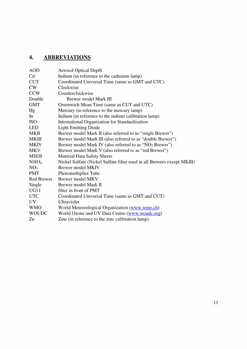
4. ABBREVIATIONS
AOD Aerosol Optical Depth
Cd Indium (in reference to the cadmium lamp)
CUT Coordinated Universal Time (same as GMT and UTC)
CW Clockwise
CCW Counterclockwise
Double Brewer model Mark III
GMT Greenwich Mean Time (same as CUT and UTC) Hg Mercury (in reference to the mercury lamp)
In Indium (in reference to the indium calibration lamp)
ISO International Organization for Standardization
LED Light Emitting Diode
MKII Brewer model Mark II (also referred to as “single Brewer”)
MKIII Brewer model Mark III (also referred to as “double Brewer”)
MKIV Brewer model Mark IV (also referred to as “NO2 Brewer”) MKV Brewer model Mark V (also referred to as “red Brewer”)
MSDS Material Data Safety Sheets
NiSO4 Nickel Sulfate (Nickel Sulfate filter used in all Brewers except MKIII)
NO2 Brewer model MKIV
PMT Photomultiplier Tube
Red Brewer Brewer model MKV
Single Brewer model Mark II UG11 filter in front of PMT
UTC Coordinated Universal Time (same as GMT and CUT)
UV Ultraviolet
WMO World Meteorological Organization (www.wmo.ch)
WOUDC World Ozone and UV Data Centre (www.woudc.org)
Zn Zinc (in reference to the zinc calibration lamp)

12
5. SAFETY ISSUES
5.1. Overview
There are a number of potential hazards associated the installation and operation of a
Brewer spectrophotometer. Failure to be aware of these potential hazards and take appropriate
precautions can lead to serious injury or death. If you do not clearly understand any of the safety issues discussed in this document then please contact the manufacturer or other expert for
clarification.
5.2. Material Safety Data Sheets (MSDS)
Material data safety sheets should be available at each Brewer installation, for all
chemicals and products that may release chemicals, which are used for Brewer maintenance.
Examples of chemicals and products that may be used for a typical Brewer installation include:
Table 1: Typical MSDS Information for a Brewer Station
Product
Name
Application Manufacturer
and Website MSDS Web Link
Mercury (Hg) lamp
Wavelength reference
Ushio Ushio.com
http://www.germicidal.com/dl/msds%20germ-
2007.pdf
Methanol Brewer
quartz
window and
dome
cleaner
Canadian
Alcohol
Company
N/A
http://www.bu.edu/es/labsafety/ESMSDSs/
MSMethanol.html
Windex Brewer
quartz
window and
dome
cleaner
SC Johnson
Scjohnson.com http://scjohnson.com/msds_us_ca/windex.asp
Sorbead
Orange
Chameleon
Desiccant
for drying air
inside
Brewer
Engelhard
Corporation
Engelhard.com
http://www.engelhard.com/msds/
loadDoc.aspx?FileNav=P16540
Sorbead Blue
Desiccant for drying air
inside
Brewer
Engelhard Corporation
Engelhard.com
http://www.varian.com/shared/oncy/
msds/sorbeadblue.pdf
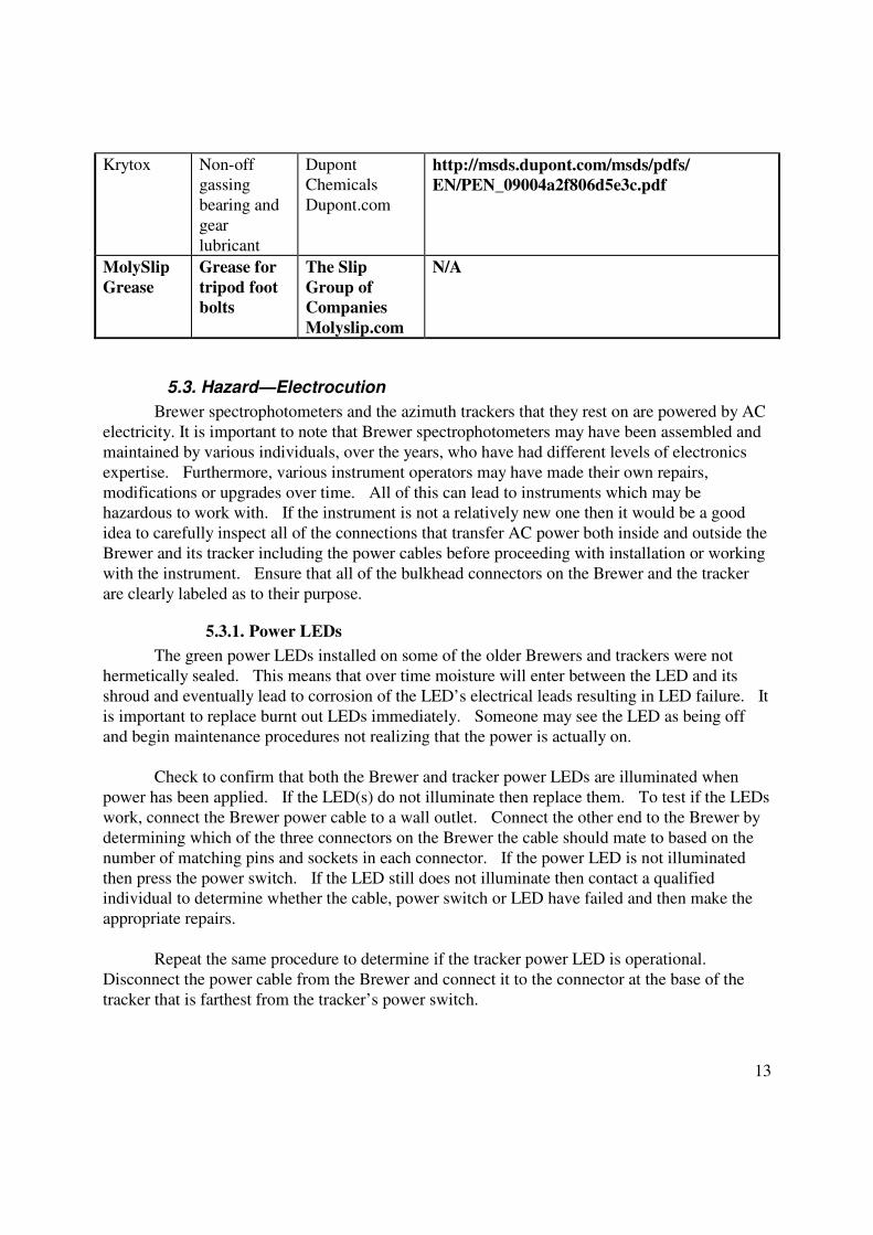
13
Krytox Non-off gassing
bearing and
gear
lubricant
Dupont Chemicals
Dupont.com
http://msds.dupont.com/msds/pdfs/
EN/PEN_09004a2f806d5e3c.pdf
MolySlip
Grease
Grease for
tripod foot
bolts
The Slip
Group of
Companies
Molyslip.com
N/A
5.3. Hazard—Electrocution
Brewer spectrophotometers and the azimuth trackers that they rest on are powered by AC
electricity. It is important to note that Brewer spectrophotometers may have been assembled and
maintained by various individuals, over the years, who have had different levels of electronics
expertise. Furthermore, various instrument operators may have made their own repairs,
modifications or upgrades over time. All of this can lead to instruments which may be hazardous to work with. If the instrument is not a relatively new one then it would be a good
idea to carefully inspect all of the connections that transfer AC power both inside and outside the
Brewer and its tracker including the power cables before proceeding with installation or working
with the instrument. Ensure that all of the bulkhead connectors on the Brewer and the tracker
are clearly labeled as to their purpose.
5.3.1. Power LEDs
The green power LEDs installed on some of the older Brewers and trackers were not
hermetically sealed. This means that over time moisture will enter between the LED and its
shroud and eventually lead to corrosion of the LED’s electrical leads resulting in LED failure. It
is important to replace burnt out LEDs immediately. Someone may see the LED as being off
and begin maintenance procedures not realizing that the power is actually on.
Check to confirm that both the Brewer and tracker power LEDs are illuminated when
power has been applied. If the LED(s) do not illuminate then replace them. To test if the LEDs
work, connect the Brewer power cable to a wall outlet. Connect the other end to the Brewer by
determining which of the three connectors on the Brewer the cable should mate to based on the
number of matching pins and sockets in each connector. If the power LED is not illuminated
then press the power switch. If the LED still does not illuminate then contact a qualified individual to determine whether the cable, power switch or LED have failed and then make the
appropriate repairs.
Repeat the same procedure to determine if the tracker power LED is operational.
Disconnect the power cable from the Brewer and connect it to the connector at the base of the
tracker that is farthest from the tracker’s power switch.
14
To prevent further damage from occurring to an LED that is not currently protected by a
hermetic seal, it is strongly recommended that a thin layer of clear silicone may be applied over the entire surface of the LED and its shroud.
5.3.2. Power Switch Terminals
It is possible that some Brewers and trackers have exposed power terminals at the back
side of their power switches. Contact with these terminals can lead to electrical shock. Ensure
that the power to the Brewer is off and that the power cable is disconnected from the Brewer. Place a generous amount of clear silicone on the back terminals of these switches if there is none
present to prevent accidental direct contact with live AC power.
5.3.3. Power Cables
Not all power cables shipped with older Brewers were UV or cold temperature-rated.
Inspect the Brewer power cables and look for any cracks in the outer cable cover. Also ensure that individual wires are not exposed at the point where the wires go into the connectors.
Replace any Brewer or tracker cables which show any sign of cracking or peeling of the cable
covering or if individual wires are exposed at any point along the length of the cables.
5.3.4. Tracker Power Terminal Strip
Ensure that the power terminal strip inside the tracker has a cover in place to isolate AC
power from accidental operator contact.
5.3.5. Maintenance and Weather
The Brewer and tracker covers should never be removed if there is any form of
precipitation. Opening the instrument during precipitation can result in both electrical shock to the operator and damage to the instrument.
Any time maintenance is to be performed on the Brewer or tracker or the cables, the
power to BOTH units should be shut off and the power cables should be removed from the wall
outlet and from the Brewer and tracker power connectors. The power connector on the tracker is
the one which is furthest away from the power switch.
5.4. Hazard—Permanent Damage to Eyesight from UV Irradiance
The Brewer contains a mercury bulb which emits a blue coloured light, and a halogen
bulb which emits a white coloured light. Both bulbs emit UV irradiance which can result in
damage to eyesight if viewed directly. Always wear UV protective goggles when working with
the lamp housing or the lamps.
5.5. Hazard—Back Injury from Handling Brewer Spectrophotometer
A single spectrometer or MKII/MKIV/MKV model Brewer has one carrying handle
suitable for carrying by one person and weighs about 30 kg or 65 lbs. A double spectrometer or
MKIII Brewer has two carrying handles suitable for carrying by two individuals and weighs 34
kg or 75 lbs. While these weights may appear to be manageable for one individual it is always safer to have two people transport the instrument.
15
It is always best to have two people carry the instrument to minimize the risk of back strain. If only one person is available for the installation then it is a little safer to remove the
Brewer cover and install the Brewer instrument on the tracker first. This makes the load lighter
and less awkward. Bolt the Brewer to the tracker and then install the Brewer cover. Refer to
Section XX on Installation of Brewer Hardware for details on how to assemble a Brewer.
5.6. Hazard—Injury due to Tripping over Cables or Tripod
Brewer cables placed on a walking surface can lead to a tripping hazard. It is best to
install the Brewer cables so that they do not lie across a walking surface. If it is not possible to
install Brewer cables below the level of the walking surface then a cable ramp should be installed
over the cables. A cable ramp also serves to protect the cables from damage.
Tripod legs also present a significant tripping hazard when walking near a Brewer.
Always walk slowly and proceed with caution around the instrument.
5.7. Hazard—Information from the Manufacturer
It is also very important to review all of the cautions expressed in the manuals which
were provided by manufacturer with the instrument. If these manuals are not available then
contact Kipp & Zonen BV for a copy of these manuals before proceeding with Brewer
installation and operation. The manufacturer’s contact information is located on the website www.kippzonen.com
16
6. INTRODUCTION
6.1. Measurement Principles and Theory
6.1.1. Ozone and sulfur dioxide
Measurements of ozone and sulfur dioxide with the Brewer spectrophotometer are based on the
Beer’s law.
6.1.2. UV
The Brewer spectrophotometers that are equipped with the UV dome are capable of measuring
the global UV irradiance.
6.1.3. Umkehr
A special type of zenith-sky observations can be done during the sunset and sunrise to record
what is called a “Umkehr effect”, the reversal of the ratio between the intensities at a short and a
long wavelengths. This observation can be interpreted by a separate computer program and a
vertical ozone profile can be deduced.
6.1.4. Aerosol optical depth
Once both the ozone and the sulfur dioxide columns are known, the residual extinction in the
Beer’s law gives an estimate of the aerosol optical depth.
6.1.5. NO2
One type of the Brewer spectrophotometer, referred to as MKIV, is capable of measuring light intensities in the visible region where nitrogen dioxide has absorption features (aprox.440 nm).
These instruments can do the direct-sun and the zenith-sky measurements of NO2 column.
6.2. The Brewer Spectrophotometer
The Brewer spectrophotometer is named after Alan W. Brewer, who began development
of the instrument at the University of Toronto. David Wardle did the original optical design and J.B. Kerr and C.T. McElroy participated in its further development. Brewer brought the idea of
the instrument to the attention of the ozone community and instigated the call for it to be made
available as a replacement to the Dobson spectrophotometer.
The first commercial prototype Brewer, sometimes referred to as the “blue Brewer”
because of the colour of its outer case, was designed and manufactured by SED Systems Ltd. in
Saskatoon, Canada. This version turned out to be unsuitable for network use for a number of reasons so Kerr, McElroy and Wardle began developing a commercial version of the Brewer
spectrophotometer in 1979 at the Experimental Studies Division of Environment Canada. This
prototype was on display at the Quadrennial International Ozone Symposium in Boulder
Colorado in 1980 where significant interest led to commercial production. Commercial
production of the first Brewer instruments was undertaken in the early 1980’s by SCI-TEC
17
Instruments Inc. in Saskatoon, Canada under license agreement with Environment Canada. In
2004 the license to build Brewers was transferred to Kipp & Zonen BV of Delft, The Netherlands. There are more than 190 Brewer instruments in over 43 countries worldwide
including Antarctica.
6.3. Brewer Models and Measurement Capabilities
There are four different models of Brewer spectrophotometers. The first single
monochromator MKII (pronounced “Mark 2”) model Brewers were built in 1982. MKII Brewers have an 1800 line per mm grating that is used in the second order to measure column
ozone and column SO2, in the UVB portion of the spectrum, as well as the vertical ozone profile
using the Umkehr technique. A few years after the first MKII’s were introduced, they were
upgraded to measure solar spectral UV irradiance as well. MKII’s are sometimes referred to as
“single Brewers” because they have a single monochromator. Solar spectral UV irradiance
measurements are made from 290 nm to 325 nm.
The first MKIV Brewer was built in 1985. MKIV Brewers have the same measurement
capabilities as the MKII instrument as well as the ability to measure column NO2. A 1200 line
per mm grating is used to measure ozone and UV in the third order and NO2 in the second order.
A filter wheel, installed between the monochromator and the PMT, allows for the automated
insertion of the appropriate order filter into the light path to switch to NO2 measurement mode,
which is performed in the visible portion of the spectrum. MKIV’s are sometimes referred to as
“dual Brewers” because they have two separate modes of operation—an ozone measurement mode and an NO2 measurement mode. Solar spectral UV irradiance measurements are made
from 290 nm to 325 nm. With a modified grating arm, MKIV Brewers can be used to measure
solar spectral UV irradiance from 286.5 nm to 363.0 nm. This type of Brewer is referred to as a
“MKIV-e” or a MKIV instrument with extended UV measurement range capability.
MKIII Brewers were first introduced in 1992 as a replacement for the MKII Brewer. The
primary advantage to the MKIII design is the use of a double monochromator. The top monochromator is used for dispersion of the incoming beam and the bottom half is used for
recombining the spectrum to present it to the photomultiplier. This virtually eliminates stray
light. Each monochromator uses a 3600 line per mm grating in the first order to measure ozone
and UV. Elimination of stray light allows the MKIII to operate without the NiSO4 and UG11
bandpass filters that are required by the MKII and MKIV models. Removal of the bandpass
filters eliminates uncertainties caused by changes in filter characteristics with time and also removes the instrument temperature dependence that is associated with the NiSO4 filter from the
calculation of ozone ad SO2. MKIII’s make the same type of measurements as MKII’s and are
sometimes referred to as “double Brewers” because they have a double monochromator. MKIII
Brewers provide high quality column ozone measurements, in the UV portion of the spectrum,
up to an airmass value of about 5.0 at an average ozone value of 300 DU or up to 1500DU of
ozone in the path that the sun’s light travels through the atmosphere. All MKIII Brewers can
measure solar spectral UV irradiance from 286.5 nm to 363.0 nm.
18
The first MKV Brewer was manufactured in 1991. The MKV Brewer is essentially the
same as a MKII Brewer but with a filter wheel installed between the spectrometer and the PMT. The filter wheel contains an order filter that allows for column ozone measurements to be made
in the “red” portion of the visible spectrum. Ozone absorption in the UV, large Rayleigh
scattering attenuation and stray light degrade the quality of ozone measurements made in the UV
portion of the spectrum with increasing airmass between the instrument and the sun. Ozone
measurements in the visible portion of the spectrum are not as strongly affected by ozone
absorption, Rayleigh scattering and stray light and as a result MKV’s are suited to the Arctic and
Antarctic regions where low solar elevation angles prevail for much of the year. MKV column ozone measurements, made in the visible portion of the spectrum, are generally acquired between
airmass values ranging from 5 to 10. MKV instruments are sometimes referred to as “red
Brewers” because they measure ozone in the red portion of the visible spectrum. Solar spectral
UV irradiance measurements are made from 290 nm to 325 nm.
Brewer model MKII, MKIII, MKIV and MKV instruments measure ozone in the UV portion
of the spectrum to an accuracy of about +/-1% when stray light is not an issue. The quality of ozone measurements made by these various models is equally accurate when the amount of ozone in path is
less than 1000 Dobson units, which is equal to 1 cm of ozone at Standard temperature and pressure.
This limit is determined by stray light and is calculated by multiplying the airmass value and the
column ozone measurement. A MKIII instrument will maintain this same level of accuracy out to
about 2000 Dobson units or 2 cm of ozone in the path. Beyond these thresholds, stray light begins to
progressively degrade the accuracies of the ozone measurements made in the UV portion of the
spectrum. MKV ozone measurements made in the visible portion of the spectrum have an accuracy of about +/-3%. The above-stated accuracies are subject to the proviso that the instruments are
operating properly and are well maintained.
Stray light for a MKIII Brewer is normally 10-7of peak intensity and in the 10-3 or 10-4 range
for a MKII, MKIV and MKV Brewers as measured using a monochromatic source. Development of
a stray light algorithm may improve MKII, MKIV and MKV Brewer column ozone measurements by
factor of 10 but never will get close to MKIII Brewer ozone measurements for three reasons. MKIII Brewers measure column ozone in the first order of the grating and do not require a NiSO4 and UG11
filter. Both of these factors increase the measured intensity relative to background noise. The
MKIII does not require a stray light correction so there is no additional uncertainty added because of
the application of this correction.
The versatility of the Brewer instrument is demonstrated by its ongoing evolution over the
years, not only in terms of the different models, but also through the other improvements made to both hardware and software. An example of a more recent software routine being tested allows the
extraction of aerosol optical depth information from direct sun measurements. Other examples
include investigation into whether the Brewer is capable of measuring tropospheric ozone, improving
the accuracy of NO2 measurements as well as ongoing improvements to the Umkehr inversion
algorithm. Brewer stray light properties are currently under investigation and may extend the
measurement range for column ozone measurements made in the UV portion of the spectrum for all Brewers.
19
6.4. Basic Component Assemblies
The basic components of a Brewer spectrophotometer are shown in Fig. XX and include a
foreoptics tube, spectrometer, photomultiplier tube (PMT), control electronics and primary and
secondary power supplies. The Brewer itself rests on a rotating pedestal, often referred to as a
“tracker” because its function is to track the sun during the day or the moon at night.
The controlling electronics in older Brewer instruments were housed in a card cage
containing seven boards which are all plugged into a motherboard located at the back of the card
cage. The photon counter board attached to the PMT counts the photonic energy from the light
source and relays this information to the controlling computer through the analog to digital
electronics board. The analog-to-digital converter board is also used for the collection of
housekeeping data like temperature and power supply voltages. Other boards in the card cage include three boards which move the various motors in the Brewer including those attached to
the tracker, zenith prism, iris, various filter wheels, wavelength-selecting micrometer and the
shutter motor. The clock board contains temperature circuitry and can be used to maintain
accurate time for the Brewer controlling software. The microprocessor board interprets and
executes commands from the controlling computer and relays the resulting instrument status and
measurement results back to the computer.
The original electronics configuration of the Brewer was maintained until 1998 when
SCI-TEC began selling the Brewer with single-board electronics. The introduction of single
board electronics also incorporated a number of improvements including built-in circuit
redundancy, improved surge suppression, shielded ribbon cables to reduce noise, and reduced
power consumption resulting in lower heat generation.
Replacement boards for the old Brewer multi-board electronics card cage are obsolete and
are no longer being manufactured. Boards that fail can usually be repaired although the
microprocessor board is one of the most difficult to repair. International Ozone Services has
developed a replacement for the microprocessor board which fits into the existing multi-board
electronics card cage. This board also has the advantage of communicating with the Brewer
computer at 9600 baud compared to the old board which communicated at 1200 baud.
The foreoptics tube is used to direct various sources of light, including light from the sun,
the sky, the horizontal diffuser, the moon or from the internal calibration lamps into the
spectrometer.
The spectrometer disperses light into its component wavelengths and directs the light
through a wavelength-selecting shutter onto the photomultiplier tube photocathode (PMT). The
photon pulse amplifier and discriminator attached to the PMT counts the photon counts from the light source and divides them by 4 to reduce the bandwidth of the signal and relays this
information along a differentially-driven twisted pair to the controlling computer via the photon
counting electronics board.
20
The first Brewer instruments that were manufactured were not fully automated nor did
they have UV measurement capability. An operator would manually configure the azimuth, zenith, iris and filterwheel positioning of the instrument for each ozone measurement. Soon
after initial production, Brewers were fitted with the quartz dome and a port mounted onto the
foreoptics to measure solar spectral UV irradiance. Motors were also added to fully automate
the operation of the Brewer.
6.5. Communication Configuration
Brewer instrument electronics were designed to support RS232 communications through
a computer’s serial port. The GWBasic Brewer software is restricted to the use of COM1 and
COM2 only. Most newer computers have USB ports instead of serial ports. It is possible to
use a USB to serial adapter to connect the Brewer data cable to computer’s USB port. It should
be noted that not all serial to USB adapter cables work with the Brewer instrument.
In the early 1990’s the capability of RS422 communication was added to the Brewer by installing a converter within the Brewer and another converter at the other end of the data cable
at the computer. RS422 increases the communication distance over data cables from 15 m or 50
ft for RS232 communications to 90 m or 300 ft. Brewers with the single board electronics have
RS422 capability built into them.
The distance between the Brewer and its computer is limited by the type of
communication system used. The official limit for an RS232 communication cable is about 15m or 50ft. RS232 communication cable lengths of up to 90m or 300ft have been used successfully
with the Brewer. The RS422/RS232 data set communications module, which may have been
installed by the manufacturer into the Brewer, extends the communication range up to 1.2 km or
4000 ft. Wireless communication systems are also available for locations where it is not
practical to run cable.
21
7. MAINTENANCE
7.1. Critical Maintenance Warnings
7.1.1. Overview
Routine instrument maintenance and care during instrument handling are required in
order to prevent potentially serious and costly damage to the Brewer instrument.
7.1.2. Photomultiplier Tube
Saturation of the photomultiplier tube (PMT) with bright light can lead to a transient
shock or permanent damage. Always power down the Brewer and disconnect its power cable
before opening the spectrometer case. It is always best to avoid opening the spectrometer cover
unless absolutely necessary to prevent excess light from entering the PMT and dust from settling
onto the optics. If the spectrometer cover must be removed then it is best to do so in a clean
dust-free room.
7.1.3. Excess Moisture
High levels humidity inside the Brewer can lead to the permanent damage of various
optical components including the film polarizer(s) and the nickel sulfate (NiSO4) and UG11
filters. Damage to these optical components will negatively impact data quality and likely require expensive repairs and instrument recalibration.
Excess moisture can also lead to the corrosion and shorting of solder traces on the various
electrical boards, which can cause erratic behaviour of the instrument as well as operational
failure. Accumulation of water inside the Brewer from a deteriorated seal can short out the
primary power supply.
Section XX on Desiccant Check/Replacement in the Maintenance portion of this
document describes how to control the humidity level within the Brewer.
7.1.4. Optical Surfaces
Do not touch or attempt to clean any of the optical surfaces inside the Brewer, especially
the spherical mirror and the diffraction grating, which are located inside the spectrometer housing. Cleaning either the diffraction grating or spherical mirror, no matter how carefully,
will result in permanent damage to the optical surfaces and may leave them unusable.
7.1.5. Lubricants
Several components in the Brewer require lubrication for proper operation. Only non-off-gassing lubricants should be used. One such lubricant approved for use in the Brewer is
“Krytox”. Most other lubricants off-gas over time and deposit themselves on sensitive optical
surfaces.
22
7.2. Routine Maintenance
7.2.1. Overview
The Brewer requires various types of maintenance to prevent damage to the instrument
and ensure proper operation. Maintenance procedures will be described according to frequency
required. Each section provides maintenance instructions in normal font. Text in italicized
font indicates solutions to resolve problems that may occur. Note that once this maintenance
information has been reviewed, the process of filling out the Brewer Log Form (to be described below) will summarize all of the required checks and their frequencies.
A summary of maintenance checks and their frequency are listed below. This
information also appears on the Brewer Log Form so that it is always at hand for the station
operator(s).
Daily Brewer Maintenance
Confirm that the Brewer is in scheduled operation mode.
Brewer software date check
Brewer software time check
Confirm that schedule is correct
Dome and window cleaning
Make appropriate entries into Brewer Log Form
Bi-Weekly (Every two weeks) Brewer Maintenance
Desiccant check/replacement
Steps per revolution check
Sighting check on sun (moon when sun not available during Arctic or Antarctic winter months)
Bi-Monthly (Every two months) Brewer Maintenance
Tracker drive plate cleaning
Detailed notes on the summary list shown above follow below.
7.2.2. Brewer Log Form
Reference is made to the “Brewer Log Form” rather than the “Station Log Form” because instruments can be moved from one station to another and because the information on the Log
Form is primarily related to the Brewer instrument and not the station.
The purpose of the Log Form (refer to Appendix XX for a sample Log form) is to
document all human interaction with the Brewer spectrophotometer system including its control
computer. The Log Form is ideally an electronic document that facilitates copying, backup,
transfer and archival. The form itself would ideally exist within the Brewer directory structure so that if the Brewer software were to be copied or transferred to another computer the Brewer
Log Form would be copied or transferred at the same time.
23
Key elements of a Log Form include:
• Contact information—experts who are available to assist Brewer operators.
• Space for the operator to note all routine checks and maintenance performed.
• A summary of procedures required to perform all routine maintenance along with
maintenance frequencies.
• An area to Log all system changes, upgrades, errors etc. including the date, time and initials
of person who noted the condition or performed the work.
The form shown in the Appendix is set up so that it can be readily printed on a single
sheet of paper or displayed entirely and legibly on a computer screen all at once. The Log Form
represents one month of information per worksheet. One Microsoft Excel workbook file can
easily hold many years worth of data.
If a station uses various schedules during the course of a year then it is a good idea to
enter the name of the schedule in the day entry of the appropriate monthly worksheet in advance
to remind the station operator of the change in schedule.
One possible naming convention for the Log Form spreadsheet file is “Log###
YYYY.xls” where “###” is the three digit Brewer serial number and “YYYY” is the four digit year.
7.2.3. Daily Maintenance
7.2.3.1. Confirm that the Brewer is in Scheduled Operation Mode
Ensure that Brewer is in scheduled operation mode. This can be confirmed by noting the
information in the second line of the software window header. During scheduled operation a
two-letter short form of the measurement name is followed by the name of the schedule in use.
If the message “Brewer not responded 5 times” or some other message indicating
communication failure appears in the center of the software window then refer to Section XX in
Appendix XX for the diagnostics procedure to resolve this issue.
If the Brewer is on menu (as indicated by the word “menu” located in the second line of
the software window header) then check the current day’s B-file to determine why scheduled
operation was aborted. If there is no indication for the reason for failure in the current day’s B-
file then check the end of the previous day’s B-file to ensure that “ed” is the last piece of
information in the file. An “ed” indicates that the file was closed properly at the end of the day.
The primary reasons for the software aborting scheduled operation are: a) the lamp intensity of
either the mercury or standard lamps was below the acceptable threshold (“lamp not found”
message), b) there was an azimuth tracker or zenith prism zeroing failure (“azimuth/zenith
zeroing failure” message), or c) someone pressed the “home” key and did not return the
software to scheduled operation mode. If the current and previous day’s B-files do not indicate
why scheduled operation was aborted then type the command string “pdrefrhphgpf” and press
“Enter”. Once this command string has completed execution check the B-file to determine if
24
there were any errors logged. If there were no errors logged then type “skc” and press “Enter”
to display the list of available schedules. Type in the name of the schedule that was in use
before scheduled operation was aborted (refer to the Log Form) and press “Enter” to resume
scheduled operation. If the error message refers to a lamp intensity problem or a zeroing
failure then refer to Appendix XX for the diagnostics procedure to follow to resolve these issues.
7.2.3.2. Brewer Software Date Check
Check the calendar day as well as the Julian day. Note that the displayed calendar day changes to the next day at Greenwich Mean Time 00 hours. The displayed Julian Day changes with the
change of the local day as determined by the sun; not the time of day. Confirm that the date is
correct using a date and time reference such as that at the National Institute for Standards and
Technology at www.time.gov and select the UTC time zone.
If the date is incorrect then refer to the Log Form to note the name of the schedule that is
currently in use. Press the “Home” key to exit scheduled operation and go to the menu list. Type
“da” and press “Enter” to change the date. Enter information as prompted (two digit day, two digit
month and two digit year). If the date was wrong then confirm that the time is correct as described
below. When done type “skc” and press “Enter” to display the list of available schedules. Type in
the name of the schedule that was in use before scheduled operation was aborted and press “Enter”.
7.2.3.3. Brewer Software Time Check
Check the C.U.T. value in the Brewer program window. (C.U.T. = U.T.C. = Coordinated
Universal Time = G.M.T. = Greenwich Mean Time). Confirm that the time is correct to within +/- 5
seconds using a C.U.T. date and time reference such as that at the National Institute for Standards and
Technology at www.time.gov and select the UTC time zone.
If the time is incorrect then refer to the Log Form to note the name of the schedule that is
currently in use. Press the “Home” key to exit scheduled operation and go to the menu list. Type
“ti” and press “Enter” to change the time. Enter the information as prompted. When done type
“skc” and press “Enter” to display the list of available schedules. Type in the name of the schedule
that was in use before scheduled operation was aborted and press “Enter”.
7.2.3.4. Confirm that Schedule in use is Correct
If multiple schedules are in use during the course of a year then confirm that the Brewer is running the correct schedule for the given day of the year. The name of the schedule currently in use
appears on the second line of the program window after the two-letter short-form name of the current
measurement.
If the schedule is not correct then press the “Home” key to exit scheduled operation and go to
the menu list. Type “skc” and press “Enter” to display the list of available schedules. Type in the
name of the correct schedule and press “Enter”.
25
7.2.3.5. Dome and Window Cleaning
Clean the entire UV dome and the entire zenith prism window using a non-abrasive tissue
for optical surfaces moistened with methyl alcohol.
Remove snow from the window and dome using a soft bristled non-abrasive brush. A thin layer of ice may be removed by very gently scraping (not chiseling) the glass surface with a
plastic car window type scraper. A thicker layer of ice may be removed by using gentle heat
from a blow dryer.
7.2.3.6. Fill Out the Brewer Log Form
Make entries into the station Log Form as required. A sample station Log Form appears in Appendix XX.
7.2.4. Bi-Weekly Maintenance (every two weeks)
7.2.4.1. Desiccant Check/Replacement
The nickel sulfate filter is very sensitive to humidity and changes its optical
characteristics when subjected to high levels of humidity resulting in unstable standard lamp test
results. Over time, excess moisture in the Brewer can cause damage to the nickel sulfate, UG11
and polarizing filters resulting in a degradation of data quality. High moisture levels can also cause shorting between traces on the various electronics boards resulting in erratic instrument
operation or operational failure. A description of two methods for controlling moisture within a
Brewer spectrophotometer along with their respective check/replacement procedures follows.
Typical Desiccant Drying System
The most commonly used type of drying system involves two desiccant systems that work
together to keep the internal components dry. The first desiccant system is the “breathing” system and consists of a lexan cylinder of desiccant that is attached to a tube connected to a hole
in base of the instrument or alternatively connected directly to an opening at the base of the
instrument without the use of a tube. This breathing system serves to dry air that passes into and
out from the instrument due to changes in atmospheric temperature or pressure compared to
internal temperature or pressure.
The second desiccant system is simply a bag or other container of desiccant that is typically placed over the secondary power supply (or other free space within the instrument) and
serves to dry the internal space of the instrument. This second system helps to remove moisture
that enters the instrument from one of the various seals, which may have developed a leak. It
also helps with the drying of the interior space each time the Brewer cover is removed—for
example, during desiccant check and replacement.
There are several types of desiccant media that are typically used in the Brewer. The first and least desirable type is desiccant that is designed for single use only (ex. Calcium Sulfate).
This desiccant is typically blue in colour when fresh and turns pink when expired. This type of
26
desiccant is not preferred because it often breaks down into a powder when saturated with
moisture. This powder can settle on instrument optics.
There are typically several desiccant media types whose moisture capacity can be
regenerated (almost indefinitely) by heating the media to release the moisture. The first of these
types consists of self-indicating beads and turns from a dark blue colour, when fresh, to a pink
colour when saturated (ex. “Trochenperlen”, “Sorbead Blue” or “Sorbead Orange Chameleon”).
To regenerate this desiccant, heat it to 140 degrees Celsius (not exceeding 180 degrees Celsius)
for a few hours or so depending on moisture content. Once dry, the desiccant needs to be placed into a dry airtight container. A second type of desiccant often used in the Brewer consists of
small beige-coloured beads and does not change colour but rather contains a separate strip of
indicator paper in the desiccant tube that turns from blue when dry to pink when moist. The best
of these desiccant media is the one that is self-indicating so that an operator can easily assess the
state of all of the desiccant in the container, not just the desiccant adjacent to the strip.
The least desirable desiccant media type is the type that is supplied in a closed opaque packet. These packets typically require a desiccant indicator card to be placed somewhere in the
instrument in order for the operator to judge the level of moisture in the instrument. An operator
has no idea as to how much drying capacity this packet has left or how long it would take to dry
in an oven. Over time most desiccant types lose their ability to be regenerated by heating. The
packet type would provide no clear indication of this situation. The indicator card, whose
measuring capability may also deteriorate with time, is often placed under the iris/entrance slit
viewing window inside the Brewer to provide an operator with an indication of the moisture level in the instrument. While this may be helpful for the operator to see what the card indicates
without taking off the Brewer cover it should be noted that at least one of the manufacturers of
these cards suggests that the card not be placed in direct sunlight. Heating the card in the
sunlight might burn off the moisture from the indicator and thus provide misleading information.
In this case it would be best to check the card on a cloudy day or even better, cover the viewing
window so that sun does not normally enter the instrument. Note that all Brewers referred to as
“MKIV” or “Dual” or “NO2” as well as those referred to as MKV or “Red” Brewers should have an opaque cover placed on the iris/entrance slit viewing window because diffuse visible light can
enter the viewing tubes and contaminate NO2 or red spectrum ozone measurements that are made
in the visible portion of the spectrum.
To check the condition of the desiccant containers inside the Brewer:
1. Press “Home” to abort scheduled operation and wait until the software displays its menu.
2. Place a protective plastic cap over the UV dome. 3. Remove the Brewer cover and examine desiccant condition or indicator condition.
4. Replace any desiccant that indicates that it is more than 50% expired or if the Brewer internal
humidity is above 50%.
5. Re-install the Brewer cover.
6. Remove the protective plastic cap from the UV dome.
7. Type “skc” and press “Enter” to display the list of schedules.
27
8. Type in the name of the schedule currently in use and press “Enter” to resume scheduled
operation. 9. Make the appropriate entry into the Log Form indicating the date that the desiccant was
checked/replaced, the percentage expired and a notation indicating if the desiccant was
replaced.
10. Regenerate the desiccant as specified by the manufacturer.
Advanced Drying System
A less commonly used but generally better moisture control system involves the removal of the above-mentioned desiccant tube and tray/packet systems and rather forces dry air or dry
nitrogen into the instrument under very low pressure. The flow of dry gas is adjusted to a level
that provides a slight positive pressure within the instrument so that moist air is never drawn into
the instrument. Dry air or dry nitrogen can be provided from a gas cylinder. Dry air can also be
made by pumping ambient air through a desiccant container.
When using a gas cylinder the only requirement is to periodically monitor tank pressure to ensure that it is still capable of providing dry gas to the Brewer. Checking or changing of the
desiccant in a system that uses ambient air is best done when the desiccant is about 50% expired.
Again, the best desiccant to use for this system is one that is self-indicating for the reasons
mentioned above.
The significant advantage to the advanced drying system is that it does not require
interruption of Brewer operation and removal of the Brewer cover, which introduces moisture and dust into the instrument.
Note: If desiccant is found to be completely or almost completely expired then it is
likely that one of the seals inside the instrument has failed. Bring the Brewer indoors
immediately to prevent damage to the instrument and correct problem—see Appendix XX on
Brewer Seal Maintenance, Diagnostics and Repair/Replacement.
Note: Most spectrometer cases have a desiccant holder mounted on the case. It is best
to empty this container and not use it since it may encourage opening the case and to check and
change it periodically. It is best to avoid opening the spectrometer case unless absolutely
required to prevent moisture from entering the spectrometer and dust from settling on the optics.
If the desiccant tube and box are properly maintained then the spectrometer case will remain dry.
7.2.4.2. Steps Per Revolution Test
The steps-per-revolution test is used to determine the number of steps in one revolution
of the azimuth tracker. The tracker first moves counter-clockwise to find its reference position.
Then it will move clockwise and count the number of steps taken to reach its reference position.
When completed the computer indicates both the new and current steps per revolution values.
The number of steps per revolution is typically about 14670 steps.
28
To run this test press “Home” to go to the menu. Type “sr” and press “Enter”. Log the
new steps per revolution value into the Log Form. If the new value is within 5 steps of the most recent previous value then press “y” to accept the new value.
If the new value is greater than 5 steps from the most recent previous value in the Log
Form then repeat the test two more times to determine if the new results are both within 5 steps
of the first test. If the three measurements are not all within 5 steps of one another then clean
the tracker azimuth drive disk as described below in the “Monthly Maintenance” section on
“Azimuth Drive Plate Cleaning”. Log the disk cleaning in the Log Form. After the disk has
been cleaned repeat the steps per revolution test two times to determine if the new results are
both within 5 steps of each other. If the two measurements are not within 5 steps of one another
then refer to Appendix XX for information on checking and adjusting drive plate tension. After
tension check and adjustment repeat the steps per revolution test two more times to determine if
the new results are both within 5 steps of the first test. If the two measurements are not within 5
steps of one another then the disk may be out-of-round and require replacement.
7.2.4.3. Sighting the Brewer on the Sun
Note: When the daily minimum solar zenith angle is less than 86 degrees then it is better
to perform a moon sighting. The daily minimum solar zenith angle can be determined by noting
the value of the zenith angle, as displayed on the top right hand corner of the Brewer window just
below the software version, near solar noon. An alternate way to do this is to use the “sa”
command (refer to the section on “Brewer Commands” above). Refer to the section below on “Sighting the Brewer on the Moon” when the daily minimum solar zenith angle is greater than 85
degrees.
The Brewer orientation procedure during installation requires the approximate alignment
of the north sticker on the tracker to “true north”. The Brewer will use the solar ephemeris
routine in its software to calculate where the sun is. The software will then point the Brewer to
where it thinks the sun is based on the year, Julian day, time of day and the latitude and longitude that were entered by the operator as well as on the default value of the north correction and
horizon correction in the instrument constants file.
The Brewer needs to be manually targeted on the sun to determine its north and horizon
correction values. The north correction is used to correct for the difference between the
orientation of the instrument on the ground when it was installed compared with the “true north”
orientation. The horizon correction corrects for the difference between the number of steps between the zenith drive reference position to where the software believes the horizon is
compared to the zenith drive step position where the horizon is determined to be from the
sighting.
It is best to perform sun sightings as close to solar noon as possible. This ensures that
the Brewer is tracking as good as possible during the portion of the day when the solar elevation is near its maximum and direct sun ozone measurements are of the highest quality. Atmospheric
scattering of sunlight is reduced with lower solar airmass values thus reducing contamination of
29
direct sun measurements by scattered light. It is also good to periodically check the Brewer
sighting at other times during the day. Ideally one good sighting is all that is required to keep the Brewer tracking correctly almost indefinitely. In reality, however, changes in the various
levels and alignments within the instrument may cause the quality of tracking to deteriorate
progressively from the time of day that the sighting was taken. Please refer to Appendix XX to
diagnose the reason for the deterioration in the quality of tracking as the Brewer moves further
away from the time that the sighting was taken.
It is assumed that the Brewer latitude and longitude (in degrees) are accurate to two decimal places (as can be determined by a GPS device). Coordinate in current use can be
determined by pressing “Home” to go to menu. Type “pdpopf” and press “Enter” to print
currently used constants to the D-file. Examine the latitude and longitude information at the end
of the D-file. If these values are not accurate to two decimal places then refer to Section XX on
Brewer configuration.
To perform a sun sighting: 1. Press the “Home” key to go to the menu.
2. Confirm that the date is correct and that the time is accurate to the second.
3. Type “ze” to zero the zenith motor and eliminate any accumulated step discrepancy.
4. Note—this step can be omitted if the steps per revolution test was completed immediately
before this sighting process. Type “sr” to determine the number of steps per revolution and
to zero the azimuth motor and eliminate any accumulated step discrepancy. Log the new
steps per revolution value into the Log Form. If the new value is within 5 steps of the most recent previous value then press “y” to accept the new value. Refer to the section above
entitled “Steps per Revolution Test” if the new result is not within 5 steps of the most recent
previous result.
5. Type “si” and press “Enter” to activate sun sighting mode.
6. Go to the Brewer and look into the Iris Viewer to confirm that the sun light is passing
through the iris. Ensure that you are not blocking the sun light from entering the quartz
window. If the sun’s image appears on the iris surface or the Brewer is not oriented toward the sun then use the four sighting push buttons to move the sun’s image into the center of the
iris opening so that the sunlight can pass on to the entrance slit.
7. Look into the Entrance Slit Viewer to confirm that the sun’s image is centered uniformly over
the entrance slit. Correct any offset of the sun’s image from the slit by using the sighting push
buttons.
8. Go to the computer and press the “Ctrl” and “End” keys at the same time to exit sighting
mode. 9. Record the date, time and the new sighting corrections into the Log Form. Then press “y” to
accept the new sighting values.
10. Type “skc” at the menu prompt and type in the correct schedule name and press “Enter” to
resume scheduled operation.
If the north correction has changed by more than 10 steps or the horizon correction has changed by more than 5 steps from the previously recorded corrections then repeat the above
30
steps again to confirm that there is a significant change compared to the previously recorded
values. If the change is more than 10 steps for the north correction or 5 steps for the horizon correction then refer to Appendix XX to diagnose and resolve this problem.
7.2.4.4. Sighting the Brewer on the Moon
Note: When the daily minimum solar zenith angle is greater than 85 degrees then it is
better to perform a sun sighting. The daily solar minimum solar zenith angle can be determined
by noting the value of the zenith angle, displayed on the top right hand corner of the Brewer window just below the software version, near solar noon. An alternate way to do this is to use
the “sa” command (refer to the section on “Brewer Commands” above). Refer to the section
above on “Sighting the Brewer on the Sun” if the daily minimum solar zenith angle is less than
86 degrees.
The Brewer orientation procedure during installation requires the approximate alignment
of the north sticker on the tracker to “true north”. When the Brewer is run for the first time in a new location, it will use the lunar ephemeris routine in its software to determine where moon is
and then point the Brewer to where it thinks the moon is based on the year, Julian day, time of
day and the latitude and longitude that were entered by the operator as well as on the default
value of the north correction and horizon correction in the instrument constants file.
The Brewer needs to be manually targeted on the moon to determine its north and horizon
correction values. The north correction is used to correct for the difference between the orientation of the instrument on the ground when it was installed compared with the “true north”
orientation. The horizon correction corrects for the difference between the number of steps
between the zenith drive reference position to where the software believes the horizon is
compared to the zenith drive step position where the horizon is determined to be from the
sighting.
It is best to perform moon sightings as close to the moon’s upper transit as possible. This ensures that the Brewer is tracking as good as possible during the portion of the day when
the moon elevation is near its maximum and focused moon ozone measurements are of the
highest quality. Atmospheric scattering of moonlight is reduced with lower lunar airmass values
thus reducing contamination of focused moon measurements by scattered light. It is also good
to periodically check the Brewer sighting at other times during the day. Ideally one good
sighting is all that is required to keep the Brewer tracking correctly almost indefinitely. In
reality, however, changes in the various levels and alignments within the instrument may cause the quality of tracking to deteriorate progressively from the time of day that the sighting was
taken. Please refer to Appendix XX to diagnose the reason for the deterioration in the quality of
tracking as the Brewer moves further away from the time that the sighting was taken.
It is assumed that the Brewer latitude and longitude (in degrees) are accurate to two
decimal places (as can be determined by a GPS device). Coordinate in current use can be determined by pressing “Home” to go to menu. Type “pdpopf” and press “Enter” to print
currently used constants to the D-file. Examine the latitude and longitude information at the end
31
of the D-file. If these values are not accurate to two decimal places then refer to Section XX on
Brewer configuration.
To perform a moon sighting:
1. Press the “Home” key to go to the menu.
2. Confirm that the date is correct and that the time is accurate to the second.
3. Type “ze” to zero the zenith motor and eliminate any accumulated step discrepancy.
4. Note—this step can be omitted if the steps per revolution test was completed immediately
before this sighting process. Type “sr” to determine the number of steps per revolution and to zero the azimuth motor and eliminate any accumulated step discrepancy. Log the new
steps per revolution value into the Log Form. If the new value is within 5 steps of the most
recent previous value then press “y” to accept the new value. Refer to the section above
entitled “Steps per Revolution Test” if the new result is not within 5 steps of the most recent
previous result.
5. Type “sim” and press “Enter” to activate moon sighting mode.
6. Go to the Brewer and look into the Iris Viewer to confirm that the moon light is passing through the iris. Ensure that you are not blocking the moon light from entering the quartz
window. If the moon’s image appears on the iris surface or the Brewer is not oriented
toward the moon then use the four sighting push buttons to move the moon’s image into the
center of the iris opening so that the moonlight can pass on to the entrance slit.
7. Look into the Entrance Slit Viewer to confirm that the moon’s image is centered uniformly
over the entrance slit. Correct any offset of the moon’s image from the slit by using the
sighting push buttons. 8. Go to the computer and press the “Ctrl” and “End” keys at the same time to exit sighting
mode.
9. Record the date, time and the new sighting corrections into the Log Form. Then press “y” to
accept the new sighting values.
10. Type “skc” at the menu prompt and type in the correct schedule name and press “Enter” to
resume scheduled operation.
If the north correction has changed by more than 10 steps or the horizon correction has
changed by more than 5 steps from the previously recorded corrections then repeat the above
steps again to confirm that there is a significant change compared to the previously recorded
values. If the change is more than 10 steps for the north correction or 5 steps for the horizon
correction then refer to Appendix XX to diagnose and resolve this problem.
7.2.5. Bi-Monthly (every two months)
7.2.5.1. Azimuth Drive Plate Cleaning
A friction interface inside the tracker is used to transfer power from the tracker motor to
the azimuth drive plate to rotate the Brewer. The stainless steel drive shaft connected to the
motor is tensioned against the aluminum drive plate. Normal movement of this drive system
causes microscopic aluminum particles to be worn off of the drive. These particles need to be
cleaned off every two months. Failure to clean the drive plate causes the particles that are worn
32
off of the plate to become larger and larger over time until they appear as flakes of aluminum.
These flakes then score the surface of the drive plate edge. The wear on the drive plate becomes progressively worse and results in permanent damage to the plate—it becomes “out of round”
and will require replacement. Failure to replace a worn drive plate will result in poor tracking
and both less “acceptable” data and lower quality data.
To clean the drive plate:
1. Press the “Home” key to abort scheduled operation.
2. Power down the tracker using the switch on the side of the tracker—the Brewer can be left powered. The stepper motor in the tracker allows for free rotation of the Brewer once the
tracker is turned off.
3. Remove the back cover of the tracker. The “back of the tracker” refers to the side of the
tracker that has the cover that is furthest from the tracker’s power switch.
4. Note roughly the Brewer’s current position. Slowly rotate the Brewer counter-clockwise to a
North position. Clean the tracker drive plate edge using a non-abrasive tissue or cloth
moistened with methyl alcohol while slowly moving the Brewer clockwise to North in small increments (a full 360 degree clockwise rotation). At each rotational increment, clean the
plate until a fresh portion of the tissue or cloth no longer removes any grayish coloured
deposit from the plate edge. During tracker rotation, be careful not to break the string that
connects the large post in the center of the tracker to the internal shut off switch. This switch
exists to prevent the tracker from winding up and breaking the power and data cables if the
tracker moves beyond its zero position (in either the clockwise or counter-clockwise
direction). If this string is broken then it must be replaced. Refer to the section on “Tracker Shutoff String Replacement” below under “Unscheduled Maintenance”.
5. Manually rotate the Brewer counter-clockwise to a position roughly near where it was before
the tracker was powered down.
6. Re-install the tracker cover after ensuring that each of the spacers on the cover bolts are
screwed in toward the head of the bolts. The bolts contain an “undercut” portion where
there are no threads. The washers must be rotated down into this area in order for the tracker
cover seal to mate properly with the tracker body. 7. Power up the tracker.
8. Type the “az” command at menu and press “Enter” to eliminate the Brewer’s step
discrepancy from the drive plate cleaning process.
9. Type “skc” and press “Enter”.
10. Type in the name of the current schedule in use and press “Enter” to resume scheduled
operation.
11. Make the appropriate entry into the Log Form indicating the date that the drive plate was cleaned.
Note: While it is recommended that this cleaning be performed at least every two months, it is much
better to perform this cleaning more frequently if the drive plate is dirty. A drive plate that is very
dirty every two months is likely an indication that the drive tension requires adjustment. Refer to the
“Tracker Drive Plate Tension Adjustment” in Appendix XX to correct this problem.
33
It is recommended that when a drive plate cleaning is required that it be performed
immediately before other bi-weekly maintenance procedures. This will allow for the plate cleaning to be followed by a steps per revolution test and then a sighting that will help to ensure
optimum tracking.
7.2.6. Unscheduled Maintenance
7.2.6.1. Mercury Lamp Replacement
Note: The mercury lamp emits UV radiation when it is powered on. A powered mercury
lamp will emit a blue coloured glow. Always wear UV protective goggles when working
with the mercury lamp.
Mercury lamps typically require replacement after one and a half to three years depending
on the quality of the lamp and frequency of lamp use. Lamp test failure can result either from
lamp burnout or from degradation of the lamp intensity that occurs as the mercury vapour forms
a progressively thicker deposit on the inner surface of the lamp. If lamp intensity (measured as
the difference in counts between slits one and four) is less than 498 counts then the software will first try to reset the micrometer and then repeat the mercury lamp test. If the lamp intensity
threshold is not reached for a second time then scheduled operation is aborted. Scheduled
operation will continue to be automatically aborted until the lamp is replaced.
The second column in the Hgoavg.### file in the Brewer data directory shows the
maximum lamp scan intensity for each day of Brewer operation. If the mercury lamp intensity is
in the range of a few thousand counts then the lamp should be replaced before it causes the Brewer to terminate scheduled operation.
If lamp replacement is due to filament burnout or due to low lamp intensity then skip the
instructions that follow and go directly to the instructions “To replace the mercury lamp” that
follow.
Several days prior to planned mercury bulb replacement due to low counts: 1. Insert several sunscan “sc” measurements into the schedule starting at zenith angles 66 and
lower for both the morning and afternoon periods. Refer to section XX for details on
schedule editing.
2. Examine the sunscan data to confirm that there are sufficient data points to determine the
instrument’s existing calibration step number. Refer to section XX for the procedure to
determine the calibration step number.
3. Press the “Home” key to abort scheduled operation. 4. Type in the name of the current schedule in use and press “Enter” to run the schedule with the
added sunscan measurements.
To replace the mercury lamp (refer to Fig. XX above):
1. Press the “Home” key to abort scheduled operation.
34
2. Type “co” and press “Enter” to enter a comment.
3. Type “old hg lamp” and press “Enter” to make a note in the B-file to indicate that the bulb is about to be replaced.
4. Type pdhphgslslslpf to run a mercury lamp test followed by three standard lamp tests. The
standard lamp ratios R5 and R6 are used to correct SO2 and ozone ETC values for changes in
instrument response with time. Having knowledge of these ratios immediately before and
after bulb replacement will allow for removal of any changes in R5 and R6, and subsequently
to ETCs, due solely to bulb replacement during data processing.
5. Wear UV protective goggles. 6. Close the Brewer software window.
7. Power down the Brewer using the power switch on the side of the Brewer near the quartz
zenith prism window.
8. Place a protective plastic cap over the UV dome.
9. Remove the Brewer cover.
10. The lamp housing is located below the zenith prism. The mercury lamp holder can be
removed from the lamp housing by loosening the two thumb screws located on either side of the housing and then sliding the holder out of the housing.
11. Use a non-abrasive tissue to handle mercury lamps. Unscrew the old bulb from its socket
and then install the new bulb.
12. The lamp holder contains a guide pin that helps to ensure that the holder is being installed
correctly into the lamp housing. Hold the lamp holder with the guide pin facing up. Note
the position of the lamp filament holder. The filament holder should not be directly above or
very close to being directly above the lamp filament otherwise it will reduce the light intensity as measured by the Brewer. If the lamp filament holder is directly above the lamp
filament when the guide pin is facing up then pry the chrome coloured spring clip, on which
the lamp socket is mounted, away from the lamp holder using a wide blade slot screwdriver.
Rotate the spring clip within the lamp holder until the filament holder is clearly offset from
the filament (about 30 degrees or so from the vertical). Press the spring clip back into the
lamp holder and confirm correct positioning of the filament holder. Re-insert the lamp
holder into the lamp housing while ensuring that the guide pin is fully inserted correctly into the lamp housing. Tighten the lamp screws.
13. Replace the Brewer cover.
14. Remove the protective plastic cap from the UV dome.
15. Power on the Brewer—you should hear the shutter click if you listen carefully.
16. Restart the Brewer software.
17. Type “co” and press “Enter” to enter a comment.
18. Type “new hg lamp” and press “Enter” to make a note in the B-file to indicate that the bulb has been replaced.
19. When the Brewer has finished its reset and returned to menu type pdhphgslslslpf to run a
mercury lamp test followed by three standard lamp tests.
20. Type “skc” and press “Enter”.
21. Type in the name of the current schedule with the added sunscan measurements and press
“Enter” to resume scheduled operation.
35
22. Make the appropriate entry into the Log Form indicating that the mercury lamp was changed.
Also note the date, time and initials of the individual who changed the lamp.
Several days after bulb replacement:
1. Examine the sunscan data to confirm that there are sufficient data points to determine the
instrument’s new calibration step number. Refer to section XX for the procedure to
determine the calibration step number.
2. If the new calibration step number is within +/- 2 steps different from the old one then the
lamp replacement process is complete and the following steps can be ignored. 3. Press the “Home” key to abort scheduled operation.
4. Type “cf” to access the constants file.
5. Scroll the cursor down to the entry next to “WL cal step number” and enter the new value.
6. Press the “Ctrl” and “End” keys at the same time to exit constants file editing mode.
7. Press “y” to write the constants to a new file.
8. Enter the new filename using the format “icfJJJYY” without using an extension and press
“Enter” 9. Type “skc” and press “Enter”.
10. The previously added sunscan measurements may be removed from the schedule.
11. Type in the name of the current schedule in use and press “Enter”.
7.2.6.2. Standard Lamp Replacement
Note: The standard lamp is a 20 Watt tungsten halogen bulb and it emits UV radiation
when it is powered on. Always wear UV protective goggles when working with the
standard lamp.
Standard lamps typically do not require replacement for many years. Lamp test failure
usually results from lamp burnout. Lamp intensity often changes significantly during the first
few hours or days of lamp use, after which there is a much more gradual decline over time due to normal lamp aging. If lamp intensity (measured as the difference in counts between slits one
and four) is less than 498 counts the standard lamp test aborts scheduled operation. Scheduled
operation will continue to be automatically aborted until the lamp is replaced.
The eleventh column in the Sloavg.### file in the Brewer data directory shows the mean
intensity of lamp scans for each day of Brewer operation. Replace the standard lamp if its
intensity is less than half of its original intensity (lamp intensity after the first few days of lamp burn-in). Also replace the lamp if lamp counts are less than 300,000. The reason to replace the
lamp if counts decrease significantly is that changes in lamp intensity can produce changes in the
wavelength spectrum emitted by the lamp. Changes in the emitted wavelength spectrum can
result in undesirable changes to the standard lamp ratios that are used to correct for changes in
instrument response with time.
To replace the standard lamp (refer to Fig. XX above):

36
1. If lamp replacement is due to filament burnout or due to low lamp intensity then skip this
step and proceed to step 5. 2. Type “co” and press “Enter” to enter a comment.
3. Type “old sl lamp” and press “Enter” to make a note in the B-file to indicate that the bulb is
to be replaced.
4. Type pdhphgslslslpf to run a mercury lamp test followed by three standard lamp tests. The
standard lamp ratios R5 and R6 are used to correct SO2 and ozone ETC values for changes in
instrument response with time. Having knowledge of these ratios immediately before and
after bulb replacement will allow for removal of any changes in R5 and R6, and subsequently to ETCs, due solely to bulb replacement during data processing.
5. Wear UV protective goggles.
6. Press the “Home” key to go to abort scheduled operation.
7. Close the Brewer software window.
8. Power down the Brewer using the power switch on the side of the Brewer near the quartz
zenith prism window.
9. Place a protective plastic cap over the UV dome. 10. Remove the Brewer cover.
11. The lamp housing is located below the zenith prism. The standard lamp holder can be
removed from the lamp housing by removing either one or two hex head bolts or one or two
thumbscrews (depending on the lamp holder version) from the rectangular plate directly
below the zenith prism opening in the foreoptics tube.
12. Always Use a non-abrasive tissue to handle standard lamps. The standard lamp is held into
its socket by a spring clip. Simply pull the lamp straight out to remove it from its socket. 13. Pick up the new bulb using a non-abrasive tissue and insert it into the lamp socket.
14. Replace the lamp holder into the lamp housing.
15. Replace the Brewer cover.
16. Remove the protective plastic cap from the UV dome.
17. Power on the Brewer—you should hear the shutter click if you listen carefully.
18. Restart the Brewer software.
19. Type “co” and press “Enter” to enter a comment. 20. Type “new sl lamp” and press “Enter” to make a note in the B-file to indicate that the bulb
has been replaced.
21. When the Brewer has finished its reset and returned to menu type pdhphgslslslpf to run a
mercury lamp test followed by three standard lamp tests.
22. Type “skc” and press “Enter”.
23. Type in the name of the current schedule in use and press “Enter” to resume scheduled
operation. 24. Make the appropriate entry into the Log Form indicating that the standard lamp was changed.
Also note the date, time and initials of the individual who changed the lamp.
37
8. HARDWARE INSTALLATION
8.1. Overview
It is important to read the entire Installation section of this manual before proceeding with
installation.
8.2. Brewer System Requirements
The computer system which controls the Brewer will require shelter from the
environment as specified by its manufacturer. Brewer data downloads as well as software
update and instrument remote control for testing or diagnostic purposes is facilitated by an
Internet connection.
Power-related requirements for the Brewer and its tracker are specified by the
manufacturer to be:
Voltage and current: 3 A @ 80 to 240 VAC or 1.5A @ 160 to 264
Frequency: 47 to 440 Hz
The Brewer’s operating temperature range has been specified by the manufacturer as 0C to +40 degrees Celsius in still air. The temperature range can be extended to -20C with an
internal heater and further to -50 degrees Celsius with a cold weather cover. A further extension
of the upper limit to the operating range may be possible by installing a white-painted aluminum
sheet mounted on standoffs above the top and front of the Brewer in such a way as not to obstruct
the zenith prism viewing window or the UV dome’s view of the horizons. This plate serves to
reflect sunlight and improve convective cooling of the instrument by allowing air to pass between
the aluminum sheet and the Brewer.
A good quality uninterruptible power supply can provide both the Brewer instrument and
its computer with stable power and reduce the incidence of operational failure due to power
outages.
The power cables for both the Brewer and its computer system should be plugged into the
same power circuit—preferably the same outlet on the same circuit--to prevent ground loops. Ground loops can cause the Brewer computer program to hang up at random intervals.
The minimum recommended surface space allocated for Brewer installation is about 2m
X 2m. It is better to allocate more space if possible as this would facilitate operator access from
all directions.
A port through a wall, roof or floor may be required to connect the power and data cable
between Brewer and computer system.
If the Brewer is to be installed at a remote station then it might be useful to consider a
means to connect to the instrument’s computer system for diagnostics purposes. There are a
38
number of remote access software packages available for remote communications. It is also
useful to have a means for the instrument to transfer its daily data files, and possibly near-real time information as well, to a centrally located server. This allowa for data backup and archival
as well as provides real time feedback on the Brewer’s operational status which can help to
minimize operational down time. This can be accomplished by having a scheduled job on the
computer which sends files from the Brewer computer via FTP for example.
8.3. Site Selection
The ideal site for a Brewer spectrometer would afford it an unobstructed view of the
whole hemisphere of the sky right down to the horizon (in all directions). The WMO (World
Meteorological Organization) specifies that no obstruction should be greater than 10 degrees for
the purpose of solar radiation measurements. The same applies for Brewer UV measurements.
In higher latitudes, where the sun spends a good deal of time at lower elevations, it would be
much more important to have a completely unobstructed horizon (especially to the south, east
and west). In some cases the availability of necessary infrastructure, such as electrical power, and shelter, as well as cost issues, may prevent fully satisfying this criterion.
The site selection criterion is less critical for Brewer direct sun ozone measurements
since these measurements are generally not performed at zenith angles greater than 72
degrees for MKII and MKIV Brewers or at zenith angles greater than 80 degrees for
MKIII Brewers. MKIV or NO2 Brewers and MKV or Red Brewers are specifically
designed to take NO2 and ozone measurements, respectively, at high zenith angles so
horizon constraints should be taken into account more carefully.
8.4. Installation Surface
The Brewer should be installed on a surface that is sufficiently rigid so that the Brewer
will not shift its position when it is walked around. Because of the shock associated with the
motion of the stepping motor that drives the azimuth mount, situating the instrument on loose material will lead to continual creep in the instrument alignment.
The installation area should be able to comfortably accommodate at least two Brewers--
one space for a permanently installed Brewer and the other space for a visiting traveling standard
Brewer for ozone calibrations. The size of the installation area should also allow for safe access
to each of the at least two Brewers in all directions. A recommended minimum surface area for two Brewers is about 2.5 m X 4.5 m or about 8 ft. by 14 ft.
The ideal orientation of the installation area would be to have the longer dimension of the
area positioned north-south. This would allow the operational Brewer to occupy the south spot
and a traveling standard Brewer to occupy the north spot without either Brewer obstructing the
other's view of the sunrise/sunset portion of the horizon. . The instrument situation is just
opposite in the southern hemisphere. Calibrations are normally done in the summer season so that the traveling standard will have a clear view throughout the day.
39
8.4.1. Building Roof Top Installation
If the building roof top is a flat surface then the tripod may be installed directly onto the
roof surface. If the surface is made of loose gravel then the tripod feet may be placed on
concrete slabs or blocks of sufficient size to prevent shifting of the slab or block if it is stepped
on.
8.4.2. Ground Installation
If the ground is not subject to freeze/thaw action and is relatively firm then the tripod feet
may be placed on concrete slabs or blocks of sufficient size to prevent shifting of the slab or
block if it is stepped on. If the ground is subject to freeze/thaw action then the Brewer should be installed onto a platform which may be constructed of wood or metal and stabilized with piles to
prevent seasonal shifting.
8.4.3. Platform installation on Building Roof Top or on Ground
A rigid platform, constructed of wood or metal is required when the ground is subject to
freeze/thaw action. It is also useful in other circumstances such as to provide the Brewer with a height advantage compared to nearby obstructions to view. A platform is also helpful when a
location is subject to blowing snow. A raised platform generally allows most low level
blowing snow to pass under the platform. Snow drifts can build up around the tracker and
tripod and prevent the tracker from rotating properly because the cables and/or the tracker
become bound in the snow.
A raised platform should be surrounded by a safety railing. A relatively safe recommended railing height is about 107 cm or 42 inches. Refer to local regulations for railing
height specifications.
If a railing is higher than 115 cm or 40 inches above the surface on which the Brewer is to
be installed then it may be necessary to elevate a Brewer’s tripod feet so that the top of the railing
is at or below the height of the bottom edge of the Brewer zenith prism window. Concrete slabs or blocks may be used to elevate the Brewer.
8.5. Brewer Spectrophotometer Assembly Instructions
Once the installation site and surface have been selected, as described above, the Brewer is
ready to be assembled.
Note: Do not plug the Brewer system into a power outlet until instructed to do so below.
1. Assemble the tripod so that it appears as shown in Fig. XX. Place the tripod over the area where
it is to be installed.
2. Place the tracker onto the tripod so that the “N” sticker on the tracker post or on the tracker base
plate (as shown in Fig. XX) are oriented toward the north in the northern hemisphere and toward
the south in the southern hemisphere. If the north stickers on the tracker post or the tracker base plate are faded or missing then remove the tracker covers and locate the north sticker on the
surface of the drive plate. Rotate the tracker on the tripod to line up the holes of the tracker post
40
base and the holes in the tripod. Attach the tracker to the tripod using three bolts as shown in Fig
XX. 3. Rotate the tripod so that the “N” sticker is facing north (or south in the southern hemisphere).
4. Place the protective plastic UV dome cover over the Brewer’s UV dome.
5. Place the Brewer onto the tracker so that both of their power switches are facing the same
direction.
6. Ensure that the Brewer’s rubber feet are centered on the tracker’s angle brackets. Loosely insert
the four bolts, by hand, through the angle brackets and into the Brewer feet. Do NOT force the
bolts into the feet. If there is ANY tightness in the movement of the bolt, before it is fully inserted up against the base of the angle bracket, then loosen the bolt and manually shift the
Brewer foot on the angle bracket by pressing on the foot until there is no tightness in screwing in
the bolt. These bolts cross-thread easily and can damage the aluminum threads. Forcing the
bolts may also prevent proper operation of the Brewer by preventing the Brewer from being
properly seated on the tracker’s angle brackets. Tighten all four bolts only when all of them have
been properly inserted into the Brewer feet.
7. There will be either two or three cables extending from the base of the tracker, not including the auxiliary power extension. Each of these cables needs to be connected to the appropriate
bulkhead connector on the Brewer. Examine the number of pins / sockets and attach each cable,
in turn, to the appropriate mating bulkhead connector on the Brewer. Attach each of the cables
coming from the base of the tracker to the Brewer. Note that the screw-on connector nuts may
appear to be tight but the connector will remain improperly attached. When the nut feels tight,
push the connector in toward the Brewer and then tighten the nut again. Repeat this process until
the connector cannot be pushed in any further and the nut is tight. 8. Attach the power cable from the power outlet to the power bulkhead connector at the base of the
tracker (the bulkhead connector furthest from the tracker power switch). Attach the data cable to
the other bulkhead connector at the base of the tracker (nearest the power switch) only if all three
of the connectors on the Brewer have a cable attached to them. Otherwise attach the data cable
directly to the remaining bulkhead connector on the Brewer.
9. It is a good idea to have a means of stabilizing the Brewer tripod against strong winds which can
upset the Brewer. The manufacturer may include a “tie-down” kit with the instrument for this purpose. The tripod feet can be bolted to a wood, metal or concrete platform. Weights can be
placed over each tripod leg. Metal straps can be placed around the tripod leg and bolted down.
Note that the Brewer should be leveled as discussed in the following section before legs are
strapped down.
10.
8.6. Leveling the Brewer Tripod
The following procedure will outline the steps required to align the azimuth axis of
rotation of the Brewer tracker with the local vertical. It is essential that the axis be vertical to
better than 0.1 degrees and that the azimuth and elevation axes be perpendicular to each other to
better than 0.1 degrees to achieve adequate pointing accuracy for all types of observations. The tracker leveling requirements are summarized in Figure XX and the leveling procedure is
outlined in Figure XX. As outlined, the procedure is based on the underlying assumption that all
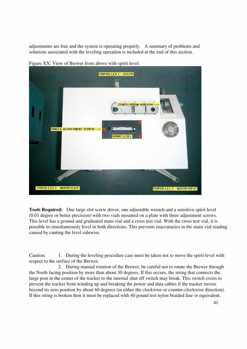
41
adjustments are free and the system is operating properly. A summary of problems and
solutions associated with the leveling operation is included at the end of this section.
Figure XX: View of Brewer from above with spirit level.
Tools Required: One large slot screw driver, one adjustable wrench and a sensitive spirit level
(0.01 degree or better precision) with two vials mounted on a plate with three adjustment screws.
This level has a ground and graduated main vial and a cross test vial. With the cross test vial, it is possible to simultaneously level in both directions. This prevents inaccuracies in the main vial reading
caused by canting the level sidewise.
Caution: 1. During the leveling procedure care must be taken not to move the spirit level with
respect to the surface of the Brewer. 2. During manual rotation of the Brewer, be careful not to rotate the Brewer through
the North facing position by more than about 30 degrees. If this occurs, the string that connects the
large post in the center of the tracker to the internal shut off switch may break. This switch exists to
prevent the tracker from winding up and breaking the power and data cables if the tracker moves
beyond its zero position by about 60 degrees (in either the clockwise or counter-clockwise direction).
If this string is broken then it must be replaced with 40 pound test nylon braided line or equivalent.
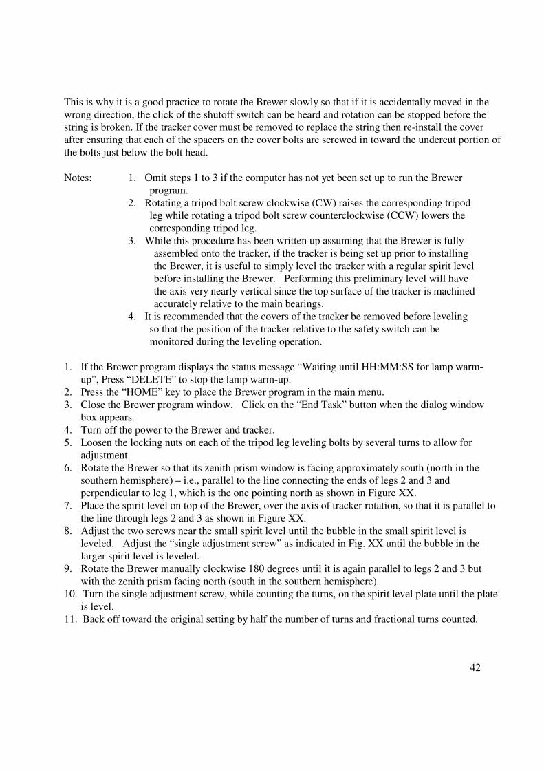
42
This is why it is a good practice to rotate the Brewer slowly so that if it is accidentally moved in the
wrong direction, the click of the shutoff switch can be heard and rotation can be stopped before the string is broken. If the tracker cover must be removed to replace the string then re-install the cover
after ensuring that each of the spacers on the cover bolts are screwed in toward the undercut portion of
the bolts just below the bolt head.
Notes: 1. Omit steps 1 to 3 if the computer has not yet been set up to run the Brewer
program.
2. Rotating a tripod bolt screw clockwise (CW) raises the corresponding tripod leg while rotating a tripod bolt screw counterclockwise (CCW) lowers the
corresponding tripod leg.
3. While this procedure has been written up assuming that the Brewer is fully
assembled onto the tracker, if the tracker is being set up prior to installing
the Brewer, it is useful to simply level the tracker with a regular spirit level
before installing the Brewer. Performing this preliminary level will have
the axis very nearly vertical since the top surface of the tracker is machined accurately relative to the main bearings.
4. It is recommended that the covers of the tracker be removed before leveling
so that the position of the tracker relative to the safety switch can be
monitored during the leveling operation.
1. If the Brewer program displays the status message “Waiting until HH:MM:SS for lamp warm-
up”, Press “DELETE” to stop the lamp warm-up. 2. Press the “HOME” key to place the Brewer program in the main menu.
3. Close the Brewer program window. Click on the “End Task” button when the dialog window
box appears.
4. Turn off the power to the Brewer and tracker.
5. Loosen the locking nuts on each of the tripod leg leveling bolts by several turns to allow for
adjustment.
6. Rotate the Brewer so that its zenith prism window is facing approximately south (north in the southern hemisphere) – i.e., parallel to the line connecting the ends of legs 2 and 3 and
perpendicular to leg 1, which is the one pointing north as shown in Figure XX.
7. Place the spirit level on top of the Brewer, over the axis of tracker rotation, so that it is parallel to
the line through legs 2 and 3 as shown in Figure XX.
8. Adjust the two screws near the small spirit level until the bubble in the small spirit level is
leveled. Adjust the “single adjustment screw” as indicated in Fig. XX until the bubble in the
larger spirit level is leveled. 9. Rotate the Brewer manually clockwise 180 degrees until it is again parallel to legs 2 and 3 but
with the zenith prism facing north (south in the southern hemisphere).
10. Turn the single adjustment screw, while counting the turns, on the spirit level plate until the plate
is level.
11. Back off toward the original setting by half the number of turns and fractional turns counted.
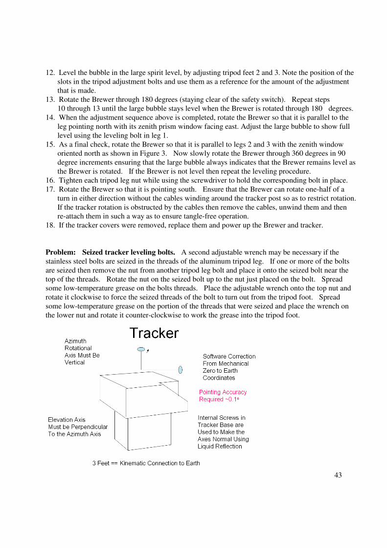
43
12. Level the bubble in the large spirit level, by adjusting tripod feet 2 and 3. Note the position of the
slots in the tripod adjustment bolts and use them as a reference for the amount of the adjustment that is made.
13. Rotate the Brewer through 180 degrees (staying clear of the safety switch). Repeat steps
10 through 13 until the large bubble stays level when the Brewer is rotated through 180 degrees.
14. When the adjustment sequence above is completed, rotate the Brewer so that it is parallel to the
leg pointing north with its zenith prism window facing east. Adjust the large bubble to show full
level using the leveling bolt in leg 1.
15. As a final check, rotate the Brewer so that it is parallel to legs 2 and 3 with the zenith window oriented north as shown in Figure 3. Now slowly rotate the Brewer through 360 degrees in 90
degree increments ensuring that the large bubble always indicates that the Brewer remains level as
the Brewer is rotated. If the Brewer is not level then repeat the leveling procedure.
16. Tighten each tripod leg nut while using the screwdriver to hold the corresponding bolt in place.
17. Rotate the Brewer so that it is pointing south. Ensure that the Brewer can rotate one-half of a
turn in either direction without the cables winding around the tracker post so as to restrict rotation.
If the tracker rotation is obstructed by the cables then remove the cables, unwind them and then re-attach them in such a way as to ensure tangle-free operation.
18. If the tracker covers were removed, replace them and power up the Brewer and tracker.
Problem: Seized tracker leveling bolts. A second adjustable wrench may be necessary if the
stainless steel bolts are seized in the threads of the aluminum tripod leg. If one or more of the bolts
are seized then remove the nut from another tripod leg bolt and place it onto the seized bolt near the top of the threads. Rotate the nut on the seized bolt up to the nut just placed on the bolt. Spread
some low-temperature grease on the bolts threads. Place the adjustable wrench onto the top nut and
rotate it clockwise to force the seized threads of the bolt to turn out from the tripod foot. Spread
some low-temperature grease on the portion of the threads that were seized and place the wrench on
the lower nut and rotate it counter-clockwise to work the grease into the tripod foot.
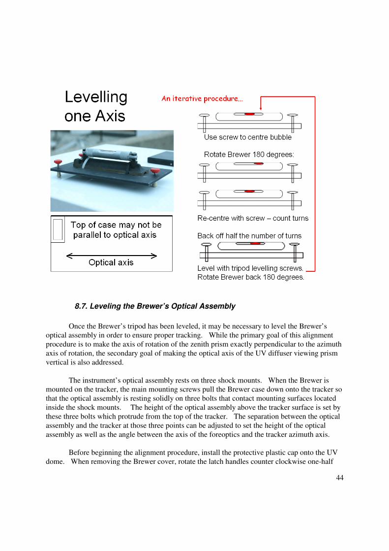
44
8.7. Leveling the Brewer’s Optical Assembly
Once the Brewer’s tripod has been leveled, it may be necessary to level the Brewer’s optical assembly in order to ensure proper tracking. While the primary goal of this alignment
procedure is to make the axis of rotation of the zenith prism exactly perpendicular to the azimuth
axis of rotation, the secondary goal of making the optical axis of the UV diffuser viewing prism
vertical is also addressed.
The instrument’s optical assembly rests on three shock mounts. When the Brewer is mounted on the tracker, the main mounting screws pull the Brewer case down onto the tracker so
that the optical assembly is resting solidly on three bolts that contact mounting surfaces located
inside the shock mounts. The height of the optical assembly above the tracker surface is set by
these three bolts which protrude from the top of the tracker. The separation between the optical
assembly and the tracker at those three points can be adjusted to set the height of the optical
assembly as well as the angle between the axis of the foreoptics and the tracker azimuth axis.
Before beginning the alignment procedure, install the protective plastic cap onto the UV
dome. When removing the Brewer cover, rotate the latch handles counter clockwise one-half

45
turn to release the latch from its catch. Then turn the latch clockwise back to their original
position, while holding the latch away from the catch, so that the latch hook is fully retracted and cannot get caught on the latch catch when the Brewer cover is lifted off. Place the cover flat on
a horizontal surface. If the cover is stood on its end or on its side there is a very high probability
that the cover will fall over and suffer damage.
The procedure used to adjust these bolts requires the removal of the tracker covers as well
as the Brewer cover. The adjustment process is made much easier if the locknuts on the tracker
bolts are installed on the inside of the tracker instead of on the outside. If the nuts are moved from the outside to the inside of the tracker longer bolts may be required to properly support the
optical assembly. Note that the bolts used to level the optical assembly must have spherical
ends machined onto them which mate with the surfaces inside the shock mounts.
Note: When the tracker bolts are properly adjusted, the Brewer optical assembly will be lifted
relative to the base of the case by a few mm (compared to the situation when the instrument is
resting on a horizontal surface rather than on the tracker) when the case is screwed down to the tracker. This force is required to ensure that the optical assembly alignment is properly
maintained. (ref. problem description at the end of this section.) However, excessive lift on the
optical assembly can cause damage to the rubber seals inside the shock mounts. A quick check
to ensure that the optical assembly is sitting properly is to push down on the assembly over each
of the three bolts in turn. If any motion can be felt, the bolts should be adjusted. This
procedure is described in the problem description at the end of this section.
Required tools: Allen keys and a high accuracy circular spirit level that fits onto the surface of
the zenith prism.
1. If the nuts on tracker-head leveling bolts are on the outside of the tracker then the Brewer
needs to be taken off of the tracker to loosen the nuts. Place an allen wrench in the socket
head of one of the leveling bolts on the inside of the tracker to hold it in place. Use a wrench to loosen the corresponding nut on the outside of the tracker by a few turns. Repeat this
process for the remaining two bolts. Place the Brewer back onto the tracker and insert and
tighten the 4 retaining screws.
2. If the nuts are on the inside of the tracker then place an allen wrench in the socket head of one
of the leveling bolts on the inside of the tracker to hold it in place while using a wrench to
loosen the corresponding nut on the bolt by a few turns. Repeat this process for the
remaining two bolts. 3. If there is reason to believe that the Brewer has not been properly aligned before, if this is the
first time the instrument has been set up on the tracker being used, or if the Brewer optical
assembly is observed to be sitting clear of the adjustment screws (as per the test in the
introduction), carry out the ‘Initial setup of the optical assembly alignment’ procedure below.
4. Place a high-accuracy circular spirit level on the surface of the UV diffuser prism.
5. Screw in one or other of the two bolts furthest away from the zenith prism to make the prism
horizontal in that axis. Screw in the third bolt (nearest the zenith prism) as needed to keep the level operating properly.
46
6. Place the circular spirit level on the surface of the zenith prism and manually rotate the brass
gear in the zenith drive system to bring the bubble as close to the centre as possible. 7. Adjust the tracker bolts until the bubble is centered within the target area. In order to ensure
that the optical assembly remains firmly on the three adjustment bolts, make the adjustment
by either screwing in the bolt nearest the zenith prism or screwing in equally the two bolts
furthest away from the prism depending on which way the optical assembly needs to be tilted.
The brass gear can be rotated manually as needed to keep the bubble in the centre of the
target. Ensure that the three adjustment bolts are never lowered such that they are not
supporting the optical assembly. 8. If the nuts are on the inside of the tracker then place an allen wrench into the socket of each
of the leveling bolts on the inside of the tracker in turn to hold it in place while using a
wrench to tighten the corresponding nuts to set the level position.
9. If the nuts on tracker head leveling bolts are on the outside of the tracker then the Brewer
needs to be taken off of the tracker to tighten the bolts. Place an allen wrench in the socket
head of the of the leveling bolts on the inside of the tracker in turn to ensure that they do not
change their adjustment while using a wrench to tighten the corresponding nut on the outside of the tracker.
10. Remove the circular spirit level from the surface of the zenith prism.
11. Place the Brewer cover back onto the Brewer. If the latches do not close properly, check to
make sure that Brewer cover is not resting on latch catch instead of slipping down behind it.
If the Brewer cover is resting on the latch catch then push the Brewer cover in toward the
Brewer in the area of the latch and off of the catch. Place the Brewer onto the tracker and
screw it down. 12. Flip the Brewer cover latch handles down to draw rain water away from the latch centre and
to prevent gradual corrosion and seizure of the latch.
13. Power up the Brewer and the tracker.
Problem: The Brewer may not be sitting properly on the optical assembly adjustment screws.
Initial setup of the optical assembly alignment.
1. The Brewer should be mounted on the tracker and fastened down with the 4 attachment
screws. The Brewer optical frame will lift up compared to the position it has relative to the
bottom of the case when it is sitting on a horizontal surface.
2. One by one, back out the three bolts until they are just free of the mounting surfaces
inside the shock mounts. This can be determined by pushing down on the optical frame over top
of each of the three screws as they are adjusted. When the screw is just free of the optical frame it will be possible to feel motion when the optical frame is pushed down.
3. With all three screws just free of their mounts, place the circular level on the Brewer.
4. Turn each screw in until the circular level just shows motion. The screws will then all be
just touching the mounts.
3. Advance the 3 bolts by 1 turns each.
4. Complete the optical assembly alignment procedure.

47
8.8. Protective Covers for NO2/Red Brewer Viewers
All Brewers referred to as “MKIV” or “Dual” or “NO2” Brewers as well as those referred
to as “MKV” or “Red” Brewers should have an opaque cover placed on both the iris and entrance
slit viewers. Alternatively, a cover can be placed on the entire lexan viewing window. The
cover(s) prevent diffuse visible light from entering the viewing tubes and contaminating NO2 or
red spectrum ozone measurements which are made in the visible portion of the spectrum. The prism in these viewers is made of glass so it absorbs UV light and thus is not a problem for
regular ozone and UV measurements. Any simple blue glass can also be used to filter out this
light. This blue glass would work for both NO2 and red ozone measurements.
8.9. Computer System Installation and Connection
Assemble the computer system as specified by the computer manufacturer. Plug the Brewer power cable into the same outlet and circuit as the Brewer computer. Connect the
Brewer data cable to the RS232 port labeled “COM1” on the back of the computer. If the
number of pins on the data cable is different from the number of sockets on the computer’s
RS232 port then an interface adapter is required. If the computer has no RS232 ports then an
RS232 card may have to be installed into the computer. An RS232 to USB interface adapter
cable may also be an option if the computer has a USB port. Note that there has not been much
experience to date using this latter option so there is no guarantee that it will work in all cases.
48
9. SOFTWARE INSTALLATION AND CONFIGURATION
9.1. Overview
It is important to install the most recent version of Brewer software since each new
version not only enhances both software and hardware operational capabilities but also
operational reliability through correction of software errors.
At the time this document was last updated International Ozone Services Inc. (IOS) has
taken it upon itself to maintain the DOS-based GWBasic version of the Brewer software. The
most recent version of the Brewer software can be downloaded from their website at
www.io3.ca.
The original software for the Brewer was written in the early 1980s using the GWBasic programming environment. The GWBasic environment is a predecessor of QBasic which in
turn has been replaced by Visual Basic. The GWbasic version of the Brewer software is still the
commonly used form of the Brewer control software. This version of the software works
relatively well within the business versions of the Microsoft operating system environment
including Windows NT and Windows XP Pro.
The GWBasic version of the Brewer program was written so that it has a “main”
component, which represents the core of the program, and a series of “routines”. This is because
GWBasic is a 64 KB interpreter. Each routine is loaded into memory and appended to the main
program as it is required and is then on completion of its execution it is overwritten by the next
required routine.
9.2. Installation of current version of the Brewer GWBasic Software
To simplify operations and installation the Brewer directory (ex. Br###, where ### is the
last three digits of the Brewer serial number) can be installed in the root directory of a hard drive.
Two subdirectories can be created under this Br### directory—one is a “Program” directory and
the other is the “Data” directory. A ### directory is created as a sub-directory in the Data
directory. Copy the GWBasic software program and routines into the Program directory. Copy the instrument’s five constant files into the ### directory.
The following directories must be created if you install in the root of disk C (Brewer
number #046 is used for this example):
C:\Br#046
C:\Br#046\program
C:\Br#046\data
C:\Br#046\data\046
Edit the Op_st.fil in the \Program directory and the Op_st.### file in the \Data\### directory, using a text editor, to ensure that the information is correct. The first line in both of
49
these files should contain only the last three digits of the Brewer serial number. The second line
in both of these files is the path to the data directory. The following is an example of how the first two lines of both of these files should look like:
046
c:\Br#046\data\
Edit the Brewer.bat file in the \Program directory using a text editor to confirm that all of the
information correct with respect to the hard disk on which the software resides as well as the Brewer program directory path. The following is an example of how the entries in this file
should appear:
c:
cd\Br#046\Program
set brewdir=c:\Br#046\Program
setdate echo on run brewer program
gwbasic main /f:10
It may be useful to copy a shortcut to the Brewer.bat file onto the computer desktop so
that the program can be started without having to find the Brewer.bat file in the program
directory.
9.3. Computer and Brewer Software Configuration for Autoboot
Refer to the computer operating system’s reference manual to configure the computer for
automatic boot up in the event of a power failure and to simplify Brewer program start up.
A copy of the Brewer.bat file can be placed into the operating system’s startup directory
so that the Brewer software can also start up the Brewer to automatically resume operation in the event of a power failure. For Microsoft Windows XP this can be achieved by placing a copy of
the Brewer.bat file into the C:\Documents and Settings\[username]\Start Menu\Programs\Startup
directory.
9.4. Start the Brewer Software
Start the Brewer software by double-clicking on the Brewer.bat icon which is located
either on the desktop or in the Brewer program directory. If the Brewer, computer, cables and
software have been installed correctly then the software will attempt to communicate and reset
the powered up Brewer in preparation for operation. When the reset cycle is completed then
main menu will appear along with a “cm>” prompt at the main menu which can be used to enter
commands to control the Brewer. If the Brewer does not reset properly or the software displays
an error message then refer to Appendix XX to diagnose the problem.
50
9.5. Setting the Buffer Delay (if required)
New computers with fast processors may require a “buffer delay” value to be entered into
the Brewer software to ensure proper communication between the Brewer and its computer. To
determine if a buffer delay is required, press the “c” key several times and watch how fast the
letters appear at the command prompt in the Brewer software window. If the response is immediate then no buffer delay is required.
If the response to repeated keystrokes is not immediate then set the buffer delay using the
“cf” command as follows:
1. Hold down the “c” key until at least one “c” appears at the command prompt. The software
may print many “c” characters on the screen because it empties the buffer all at once.
Simply press the “Backspace” key to delete all of the “c” characters except one. 2. Repeat the same process to place one “f” character after the “c”. When “cf” after the
command prompt then press “Enter” and wait for the constants file to be displayed.
3. Cursor down to the “Buffer Delay (s)” value near the end of the file and type “0.2” over the
existing entry.
4. Press the “CTRL” and “END” keys to exit the constants file. Press “n” when prompted if
you want to save the information into a new constants file.
5. Hold down the “c” key at the command prompt to determine if the display response has improved. If this process does not yield and immediate response then repeat the above steps
and increment the delay by another 0.1 and so on until the response to keystrokes is
immediate.
9.6. Brewer Time-Keeping Options
Maintaining the Brewer software window clock to within +/-5 seconds from the correct
time is important to ensure proper tracking of the Brewer instrument.
There are a few time-keeping options which may be used to maintain correct Brewer
time. The Brewer itself contains a clock card which is installed inside its card cage. The time,
as maintained by this clock card, can be set by typing the “ti” command at the main menu and
pressing the “Enter” key. This clock card contains two batteries that are used to maintain the Brewer clock in the event that there is a power failure or when the power to the Brewer has been
turned off. A second time-keeping option is to use the computer clock to update the GWBasic
environment clock. A third option is to use the computer clock which is automatically kept
correct by using some combination of hardware and/or software as discussed below.
Most computer clocks are fairly poor at keeping time and can be off by 15 seconds or
more each day. The Brewer internal clocks tend to be much better than computer clocks but still require periodic use of the “ti” command to correct any time drift beyond 5 seconds from the
correct time. The best option for keeping time is to use some means to automatically maintain
the computer clock’s time so that it is always correct. There are a number of options available to
maintain the accuracy of the computer clock. A few of these options include: a) a high accuracy
time keeping card, which is installed into the computer, b) a GPS receiver card which is installed
into the computer that polls the time from GPS satellites or c) time server software which
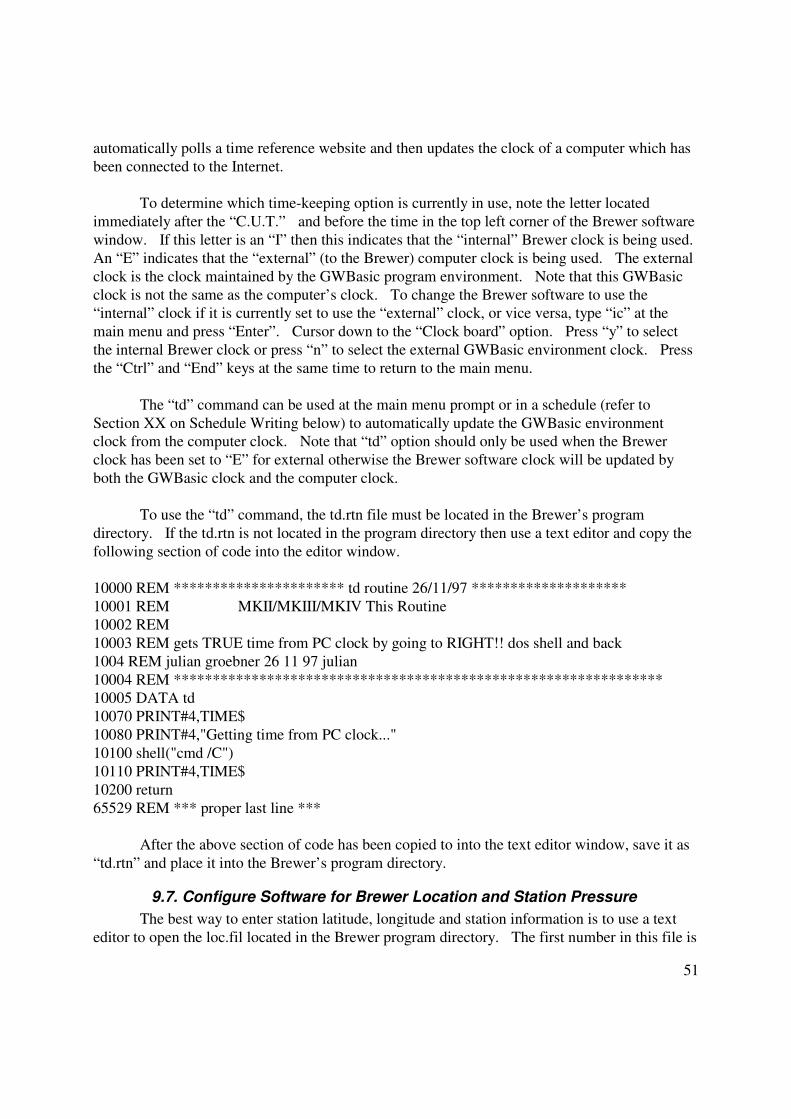
51
automatically polls a time reference website and then updates the clock of a computer which has
been connected to the Internet.
To determine which time-keeping option is currently in use, note the letter located
immediately after the “C.U.T.” and before the time in the top left corner of the Brewer software
window. If this letter is an “I” then this indicates that the “internal” Brewer clock is being used.
An “E” indicates that the “external” (to the Brewer) computer clock is being used. The external
clock is the clock maintained by the GWBasic program environment. Note that this GWBasic
clock is not the same as the computer’s clock. To change the Brewer software to use the “internal” clock if it is currently set to use the “external” clock, or vice versa, type “ic” at the
main menu and press “Enter”. Cursor down to the “Clock board” option. Press “y” to select
the internal Brewer clock or press “n” to select the external GWBasic environment clock. Press
the “Ctrl” and “End” keys at the same time to return to the main menu.
The “td” command can be used at the main menu prompt or in a schedule (refer to
Section XX on Schedule Writing below) to automatically update the GWBasic environment clock from the computer clock. Note that “td” option should only be used when the Brewer
clock has been set to “E” for external otherwise the Brewer software clock will be updated by
both the GWBasic clock and the computer clock.
To use the “td” command, the td.rtn file must be located in the Brewer’s program
directory. If the td.rtn is not located in the program directory then use a text editor and copy the
following section of code into the editor window.
10000 REM ********************** td routine 26/11/97 ********************
10001 REM MKII/MKIII/MKIV This Routine
10002 REM
10003 REM gets TRUE time from PC clock by going to RIGHT!! dos shell and back
1004 REM julian groebner 26 11 97 julian
10004 REM *************************************************************** 10005 DATA td
10070 PRINT#4,TIME$
10080 PRINT#4,"Getting time from PC clock..."
10100 shell("cmd /C")
10110 PRINT#4,TIME$
10200 return
65529 REM *** proper last line ***
After the above section of code has been copied to into the text editor window, save it as
“td.rtn” and place it into the Brewer’s program directory.
9.7. Configure Software for Brewer Location and Station Pressure
The best way to enter station latitude, longitude and station information is to use a text
editor to open the loc.fil located in the Brewer program directory. The first number in this file is
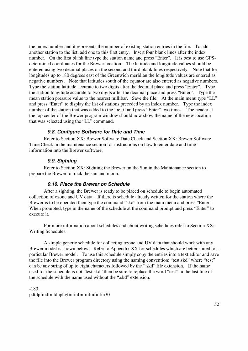
52
the index number and it represents the number of existing station entries in the file. To add
another station to the list, add one to this first entry. Insert four blank lines after the index number. On the first blank line type the station name and press “Enter”. It is best to use GPS-
determined coordinates for the Brewer location. The latitude and longitude values should be
entered using two decimal places on the second and third blank lines respectively. Note that for
longitudes up to 180 degrees east of the Greenwich meridian the longitude values are entered as
negative numbers. Note that latitudes south of the equator are also entered as negative numbers.
Type the station latitude accurate to two digits after the decimal place and press “Enter”. Type
the station longitude accurate to two digits after the decimal place and press “Enter”. Type the mean station pressure value to the nearest millibar. Save the file. At the main menu type “LL”
and press “Enter” to display the list of stations preceded by an index number. Type the index
number of the station that was added to the loc.fil and press “Enter” two times. The header at
the top center of the Brewer program window should now show the name of the new location
that was selected using the “LL” command.
9.8. Configure Software for Date and Time
Refer to Section XX: Brewer Software Date Check and Section XX: Brewer Software
Time Check in the maintenance section for instructions on how to enter date and time
information into the Brewer software.
9.9. Sighting
Refer to Section XX: Sighting the Brewer on the Sun in the Maintenance section to
prepare the Brewer to track the sun and moon.
9.10. Place the Brewer on Schedule
After a sighting, the Brewer is ready to be placed on schedule to begin automated collection of ozone and UV data. If there is schedule already written for the station where the
Brewer is to be operated then type the command “skc” from the main menu and press “Enter”.
When prompted, type in the name of the schedule at the command prompt and press “Enter” to
execute it.
For more information about schedules and about writing schedules refer to Section XX:
Writing Schedules.
A simple generic schedule for collecting ozone and UV data that should work with any
Brewer model is shown below. Refer to Appendix XX for schedules which are better suited to a
particular Brewer model. To use this schedule simply copy the entries into a text editor and save
the file into the Brewer program directory using the naming convention: “test.skd” where “test”
can be any string of up to eight characters followed by the “.skd” file extension. If the name
used for the schedule is not “test.skd” then be sure to replace the word “test” in the last line of the schedule with the name used without the “.skd” extension.
-180
pdtdpfmdfmtdhphgfmfmfmfmfmfmfm30
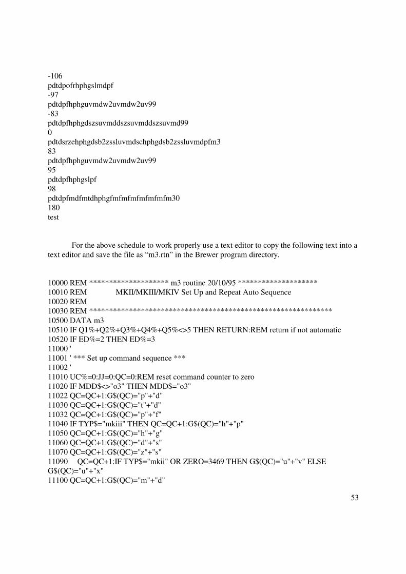
53
-106
pdtdpofrhphgslmdpf -97
pdtdpfhphguvmdw2uvmdw2uv99
-83
pdtdpfhphgdszsuvmddszsuvmddszsuvmd99
0
pdtdsrzehphgdsb2zssluvmdschphgdsb2zssluvmdpfm3
83 pdtdpfhphguvmdw2uvmdw2uv99
95
pdtdpfhphgslpf
98
pdtdpfmdfmtdhphgfmfmfmfmfmfmfm30
180
test
For the above schedule to work properly use a text editor to copy the following text into a
text editor and save the file as “m3.rtn” in the Brewer program directory.
10000 REM ******************** m3 routine 20/10/95 ******************** 10010 REM MKII/MKIII/MKIV Set Up and Repeat Auto Sequence
10020 REM
10030 REM *************************************************************
10500 DATA m3
10510 IF Q1%+Q2%+Q3%+Q4%+Q5%<>5 THEN RETURN:REM return if not automatic
10520 IF ED%=2 THEN ED%=3
11000 ' 11001 ' *** Set up command sequence ***
11002 '
11010 UC%=0:JJ=0:QC=0:REM reset command counter to zero
11020 IF MDD$<>"o3" THEN MDD$="o3"
11022 QC=QC+1:G$(QC)="p"+"d"
11030 QC=QC+1:G$(QC)="t"+"d"
11032 QC=QC+1:G$(QC)="p"+"f" 11040 IF TYP$="mkiii" THEN QC=QC+1:G$(QC)="h"+"p"
11050 QC=QC+1:G$(QC)="h"+"g"
11060 QC=QC+1:G$(QC)="d"+"s"
11070 QC=QC+1:G$(QC)="z"+"s"
11090 QC=QC+1:IF TYP$="mkii" OR ZERO=3469 THEN G$(QC)="u"+"v" ELSE
G$(QC)="u"+"x" 11100 QC=QC+1:G$(QC)="m"+"d"
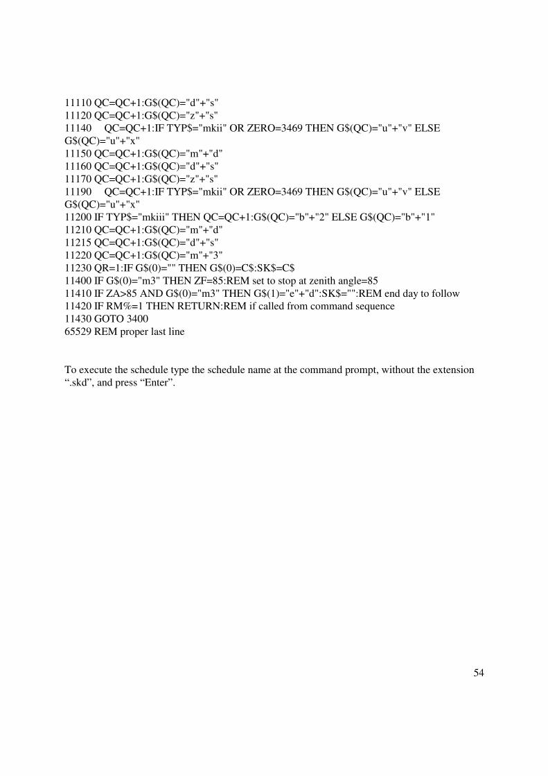
54
11110 QC=QC+1:G$(QC)="d"+"s"
11120 QC=QC+1:G$(QC)="z"+"s" 11140 QC=QC+1:IF TYP$="mkii" OR ZERO=3469 THEN G$(QC)="u"+"v" ELSE
G$(QC)="u"+"x"
11150 QC=QC+1:G$(QC)="m"+"d"
11160 QC=QC+1:G$(QC)="d"+"s"
11170 QC=QC+1:G$(QC)="z"+"s"
11190 QC=QC+1:IF TYP$="mkii" OR ZERO=3469 THEN G$(QC)="u"+"v" ELSE
G$(QC)="u"+"x" 11200 IF TYP$="mkiii" THEN QC=QC+1:G$(QC)="b"+"2" ELSE G$(QC)="b"+"1"
11210 QC=QC+1:G$(QC)="m"+"d"
11215 QC=QC+1:G$(QC)="d"+"s"
11220 QC=QC+1:G$(QC)="m"+"3"
11230 QR=1:IF G$(0)="" THEN G$(0)=C$:SK$=C$
11400 IF G$(0)="m3" THEN ZF=85:REM set to stop at zenith angle=85
11410 IF ZA>85 AND G$(0)="m3" THEN G$(1)="e"+"d":SK$="":REM end day to follow 11420 IF RM%=1 THEN RETURN:REM if called from command sequence
11430 GOTO 3400
65529 REM proper last line
To execute the schedule type the schedule name at the command prompt, without the extension
“.skd”, and press “Enter”.
55
10. DATA ACQUISITION
10.1. Overview
The Brewer software can execute various measurement, diagnostic and calibration
functions by typing the appropriate two letter command sequence at the command prompt and
pressing “Enter”.
The software also accepts a string of two-character commands for automatic execution of
the entire command string. Refer to the manufacturer’s Operator’s Manual for more detailed
information on the commands available and their function.
A schedule is simply an ASCII text file which contains a series of command strings, each
of which are executed as a function of the zenith angle specified on the preceding line in the file. Morning zenith angles are preceded by a negative sign. Schedules are invoked at the menu
prompt by typing either the “sk” command for one day only, or the “skc” command which runs
the schedule continuously.
The final line in the schedule is the name of the schedule, without a file extension, to be
run on the next day. This can either be the name of the schedule itself or the name of another schedule. This feature allows for the execution of different schedules.
The ed.rtn (end of day routine) automatically executes at the end of each day and creates a
summary of the diagnostic and measurements performed during the day.
To exit scheduled operation:
If the computer displays the message "press home to stop" then do so. If the computer displays the message "lamp warm-up" then press the “DELETE” key to abort
the warm-up and then press “HOME” to exit when prompted.
10.2. Scheduled Operation and Writing Schedules
To execute a command at solar noon type “0” as the zenith angle. Specifying a zenith
angle as “1” (if there is no 0 line before it) instructs the software to execute the following command string soon after solar noon. Specifying a zenith angle of “180” instructs the software
to execute the following command string at the time of solar midnight. Note that the command
sequences following a “0”, “1” or “180” will be executed even though none of these solar angles
are actually achievable due to latitude or season.
To write commands to the D-file, which provides a formatted version of information that
appears in the B-file, place a “pd” command immediately before the commands that are to be written. A “pf” can be used to stop the writing of information into the D-file.
56
If the next zenith angle occurring in the schedule has been achieved then the software will
continue executing its current command to completion before proceeding to the next command string. If a command string is completed before the next zenith angle in the schedule is reached
then the Brewer will sit idle and display the message “waiting until HH:MM:SS for [next
measurement]” until the next zenith angle is achieved.
A number between 1 and 99 can be placed at the end of a command string to indicate the
number of times to repeat the sequence to save writing the same commands again. Alternately,
there is a routine called au.rtn (automatic routine) which can execute a series of commands and repeat it automatically just by inserting “au” as a command in the schedule. This routine can be
be copied and given a different name so that different automatic routine command sequences can
be executed at different zenith angles. Note that the name of the new routine should be two
letters followed by the extension “.rtn” because the software parses the command strings into two
letter commands. It is also important to ensure that the name of the new file is not the same as
the name for any of the existing routines in the program directory to prevent existing files from
being overwritten. If the au routine is copied then it is important to do a search for the “au” string within the au.rtn file and change all occurrences of “au” to the new two letter name for
consistency.
10.3. Scheduling Commands
The following Tables describe the duration, frequency and recommended airmass ranges
for measurement and diagnostic commands as a function of Brewer model. Note that it is assumed that the Brewer version of software being used is 3.75f which allows simultaneous
movement of both micrometers for a multi-board MKIII Brewer.
Since instrument hardware and software configuration may not fall into one of the table
categories below or may change with time, one fairly easy way to accurately determine
measurement duration is to go to menu and run a command string containing each measurement
type separated by “td” commands (ex . pdtdhptdhgtdsltdaptddttdrstddstdzstduvtdpf).Examine the D-file and determine the time differences for timestamps preceding and following each
measurement.
10.3.1. Scheduling Measurement Commands
[Create a table for each Brewer model w and w/o new electronics for time taken for all obs.]
[Table]
Minimum Recommended Measurement Frequencies
�Specify minimum # ds #uv #zs / hr during daylight hours—specify using reasons—ex.
Statistical, satellite overpass…discuss with Volodya and Vitali. Add this info to meas duration
chart? Set up the same schedules at all sites so that data is the same at each site for a given
zenith angle. Then uv and ozone observations can be compared and other related site factors can
be studied—ex. Site altitude, window/ dome cleanliness etc. can be studied
57
10.3.2. Scheduling Diagnostic Commands
[Create a table for each Brewer model w and w/o new electronics for time taken for all obs.]
[Table]
10.4. Writing Schedules
In order to make measurements in an optimal manner, different schedules will likely have
to be written for different time periods of the year, especially for mid-latitude and high-latitude
stations, due to the significant changes to solar elevation during the course of the year. Different
schedules will also have to be written to take full advantage of different measurement capabilities
of various Brewer models.
The “sa” command can be used to display zenith angles and airmass values for both the
sun and the moon for any given day of the year as a function of time. First type the “pd”
command to log the information to the D-file and press <Enter>. Then type the “sa” command,
press <Enter> and respond to the information requested. Generally, entering “0” for the start
time, “24” for the end time and “5” minutes for the time increment provides sufficient resolution
for schedule writing. A comment can be entered at the comment prompt if desired otherwise just press <Enter>. `The tables generated using the “sa” command along with the tables above
showing measurement duration, frequencies and recommended airmass ranges.
10.5. Tips for Schedule Writing
10.5.1. Micrometer Movement
Commands which involve micrometer movement include hp, hg, sc, uv, ux, um, n2, and
o3. It is best to place commands which do not move the micrometer (ex. ds, zs, etc.) directly
after an hphg to prevent loss of data in the event that a micrometer movement issue develops and is not addressed immediately.
10.5.2. Lamp Commands
It is best to schedule an “hphg” command with sufficient frequency to ensure that
important to ensure that this string is always executed before instrument temperature changes by
3 degrees Celsius in order to compensate for temperature=induced spectrum shifts.
It is good practice to use “hphg” instead of just “hg” even for MKII, MKIV, and MKV
instruments to make schedules more generic and to prevent data degradation due to mis-
alignment of the two micrometers in the event that the schedule is ever installed on a MKIII
Brewer or shared with someone who has an MKIII Brewer.
It’s a good idea to have a take a few sl measurements at various times during the day, in
order to collect instrument response data at various temperatures.
Scheduling more than about 30 hphg commands and more than 6 sl commands is likely
excessive and will lead to premature aging and burn out of the hg and sl lamps without providing
any more useful information.
58
It is better not to place any command that measures light from the sun or sky between a
lamp warm up command (i.e., b1 or b2) to prevent light from reflecting off of the quartz window and contaminating the signal.
Newer versions of the Brewer software perform a micrometer and filter wheel #3 reset
(fr) automatically after each instrument reset (re) command. As a result, it is necessary to run an
hphg to properly position the micrometer to disperse the correct wavelengths onto the exit slits of
the spectrometer.
It is recommended that about ten standard lamp measurements be scheduled evenly
throughout each day and night so they occur at various temperatures and can be used to monitor
instrument response changes with temperature.
10.5.3. DS, ZS, FZ and UV Measurements
UV measurements at zenith angles greater than 90 degrees may contain useful information. There is likely no value in measuring UV for ze angles greater than 95 degrees.
Measurements can be taken at 90<ze<95 if the instrument has nothing else to do. The absolute
minimum is two UV measurements per hour for zenith angles less than 90 degrees and it would
be nice to have three to four measurements per hour around solar noon.
It is also useful to take DS and ZS measurements at high zenith angles. At present, we do
not use measurements taken at mu>3.5 (or 4 - depending on the site). Focused sun measurements can be used down do an airmass of 8.2 or to a zenith angle of 85 degrees. With
new algorithms that help to correct for stray light it is hoped that MKIII instruments will produce
useful ozone values to an airmass of 8.0 and that MKII, MKIV and MKV Brewers will product
useful ozone measurements in the UV down to an airmass of 5.0.
10.5.4. Focussed Moon Observations
Focussed moon (fm) observations can be contaminated by sunlight if sun is near or above
horizons so it is best not to schedule these measurements for zenith angles less than 92 degrees.
10.5.5. Umkehr Commands
A “um” command runs indefinitely so it is best to schedule desired measurement commands before it. It is better to use the u5 routine which collects the required amount of data
for umkehr processing purposes since the runtime of this command is known in order to facilitate
the scheduling of other commangs. If “um1” is typed in a schedule after an angle (and nothing
else) then only one um scan will be done.
10.5.6. CI and CZ Scans
Ci scan of entire 290 to 325 should be done say once a week. Does not have to be too
fine. Cz scan of hg line should be done at about same frequency.

59
10.6. Sample Schedules
Recommended generic sample scheds in appendix for mod/mid-lat—min rec # uv and ds
per hour for Global network. Write schedules for 20, 40, 60 and 80 degrees with min number of
ds,zs,uv,um meas. for the various seasons. Reverse for southern hemisphere.

60
61
11. ROUTINE DIAGNOSTICS
11.1. Overview
The Brewer generates a significant amount of diagnostic information during routine
operation. Results from diagnostic tests can be found on the computer screen, in the
instrument’s B-files, D-files as well as in the various average files. The information from these files can be used to determine the current operational state of the instrument as well as to address
any concerns before they begin to have negative implications for both data quantity and data
quality.
11.2. Daily Error Checks
There are three classes of errors that may occur during Brewer operation. The first class of error will result in the error message being written to the software window and immediate
failure of Brewer operation. Examples of these types of error messages include “Brewer failed
to respond 5 times” or “reset in ## seconds”, which are displayed on the screen and result from
an instrument power or communications failure.
The second class of errors result in an error message being written to the B-file at the time that the instrument was last in scheduled operation mode and cause the software to abort
scheduled operation and display the command prompt at the main menu. Examples of these
types of errors include a motor zeroing failure or a lamp not found error. These errors will cause
the Brewer software to exit scheduled operation because continued operation would not yield
useful information. As long as the software is on menu, it will create small daily B-files with
file header information only.
The third class of errors, which are not as serious, do not cause the software to exit
scheduled operation but simply generate warning messages in the B-file. One example of a
warning message results from an unrecognized character string in the schedule file. The B-files
must be examined in order for the operator to be aware of this type of error.
A software package called “BrwRprt.exe” can be used to extract error and warnings
information from B-files. This software also extracts any text from the “B-file” that does not reflect normal Brewer operation. The list of recognized text strings is user-editable. Refer to
Appendix XX for more information about this free software and on how to access it.
Please refer to Appendix XX for the procedures to deal with each type of error or warning
message. Log all types of errors into the Brewer Log Form along with the action(s) taken to
resolve them.
11.3. Weekly Diagnostic Checks
Various diagnostic parameters should be monitored in order to ensure that the Brewer is
operating optimally. Each of the following diagnostic tests topics provides the two letter
62
command used to invoke the test, the location of the diagnostic information, a brief description
of the purpose of the test, acceptable limits, and potential problems and recommendations. Software like BrwrRprt.exe can be used to extract diagnostic information from Brewer B-files as
well as from the various average files. Refer to Appendix XX on Troubleshooting for detailed
instructions on resolving any variances from recommended limits for each diagnostic parameter.
Refer to Appendix XX for more information about this free software and on how to access it.
11.3.1. Mercury Lamp Test (hg)
Information location: Mercury lamp intensity information can be found in the second column of
the Hgoavg.### file.
Purpose: Spectral shifts occur in the spectrometer as the instrument’s temperature changes.
The mercury lamp test is used to locate either the 302.15 nm or 296.73 nm mercury spectral
emission line (depending on software configuration) and then re-position the grating to disperse
the five operational wavelengths onto the spectrometer’s corresponding exit slits.
Acceptable limits: Mercury lamps last about one to three years depending on the bulb and
frequency of use. Lamp intensity gradually declines with use due to deposition of a mercury
film on the inner surface of the lamp. Lamp intensities of new mercury bulbs can range from
about 40,000 counts to about 150,000 counts, as measured by the hg routine, depending on the
sensitivity of Brewer and neutral density attenuation filter in place during the test. It is common
for mercury lamp intensity to decline by as much as 10,000 to 20,000 counts during the first few hours or days of use before starting a slower rate of decline in intensity levels.
Potential problems and recommendations: It is a good idea to replace mercury lamps once their
lamp intensity deteriorates to about 20% of their original value. At this point there is generally
not much life left in the bulbs and the intensity check performed at the beginning of each test can
cause the test to fail and the Brewer to abort scheduled operation if the lamp intensity falls below 400 counts.
11.3.2. Standard LampTest (sl)
Information location: Standard lamp R5, R6 and intensity information can be found in the ninth,
tenth and eleventh columns, respectively, of the Sloavg.### file.
Purpose: The standard lamp test is used to monitor the stability of the instrument’s response to
light over time. Standard lamp tests produce two diagnostic ratios, the R5 and R6 ratios, which
can be used to correct the instrument’s SO2 and ozone extraterrestrial coefficients respectively.
Acceptable limits: The R5 and R6 ratios should remain stable over time and remain within +/-
20 and +/-10 units, respectively, of their nominal values.
Standard lamps can last for many years depending on the bulb and frequency of use. Lamp
intensity generally decreases slowly over time and can be further reduced by the deposition of a
black or white film on the inner surface of the bulb. Lamp intensities of new standard lamps can
63
range from about 500,000 counts to about 1,200,000 counts, as measured by the sl routine,
depending on the sensitivity of Brewer and on the neutral density attenuation filter in place during the test. It is common for standard lamp intensity to decline by as much as 50,000 to
100,000 counts during the first few hours or days of use before starting a slower rate of decline in
intensity levels.
Potential problems and recommendations: It may be a good idea to replace the standard lamp if
lamp intensity declines to about 50% of its initial value. Lamp intensities below 350,000 counts
can lead to higher standard deviations in the measurement results of other diagnostic tests.
The neutral density filter in place during the test is recorded after each “sl” scan. If lamp
intensities of new standard lamp bulbs is below about 500,000 counts and the filter in place is 1
or two, stettings 64 and 128 respectively, then the neutral density filter can be reduced to the next
lowest settings, 0 and 64 respectively, using the “cf” command to increase lamp counts and also
effectively increase the useful life of the bulb.
11.3.3. A/D Information Checks (ap)
Information location: PMT high voltage and primary power supply 5 volt level information can
be found in the second and third columns, respectively, of the Apoavg.### file.
Purpose: Stability of the high voltage level supplied to the PMT and the +5 volt level from the
primary power supply are critical to proper instrument operation.
Acceptable limits: The PMT high voltage level should remain within two increments or about
+/- 22 units of its nominal value.
The +5 volt level on the primary power supply, with lamps on, should be between +4.95 to +5.10
volts.
Potential problems and recommendations: Variation in the PMT high voltage level above
acceptable limits should be investigated.
Primary power supply voltage levels below 4.8 volts can lead to erratic Brewer operation
including operational failure. The potentiometer on the power supply can be used in an attempt
to bring the +5 volt level within acceptable limits. If there is not enough adjustment available in the potentiometer to bring the +5 volt level to within acceptable limits then it is likely that
contact corrosion is the cause.
11.3.4. Dead Time Test (dt)
Information location: The high intensity dead time test results and the low intensity dead time
test results can be found in the second and third columns, respectively, of the Dtoavg.### file.
Purpose: The dead time test measures the dead time of the PMT and the photon counting
circuitry. The dead time is the time during which the PMT is not able to count a second photon

64
after the first photon has been detected. The dead time constant is used to correct for the
Brewer’s non-linear response to light. A correct response curve (counts as a function of light) would be a linear curve (i.e. counts directly proportional to level of irradiance). However, the
curve actually begins to move below the ideal at higher irradiance levels. Three percent to four
percent of the counts have to be added back to the signal at the 1 million count level (i.e., real
count rate is 3 to 4% higher than measured value at 1 million count level). About 6% of the
counts have to be added back at the 2 million count level. The ideal operating range is between
one and two million counts. The dead time correction depends on the count rate and on the dead
time itself. 30 nanoseconds (dead time constant) . 106 (count rate) = 3% correction. The
correction is calculated, using Poisson’s law, as = expλ . . . . x where λ is the dead time constant and x
is the count rate. The value in the brackets is 0.03.
Acceptable limits: The high intensity dead time test value should be within +/- 2 ns of the
current dead time setting in the instrument’s constants file.
The high and low dead time means should agree to within an acceptance tolerance of two high
intensity dead time test standard deviations and lie in the range of 30 to 45 ns.
Acceptable standard deviation values for dead time tests are up to 2.5 for high intensity and up to
20 for low intensity.
Standard deviation values for high and low intensity dead time tests can be found in the D-files.
Potential problems and recommendations: Failure to satisfy the acceptable dead time test
criteria suggest that the shutter motor operation, high voltage circuitry and the photon counting
circuitry should be examined. Variable dead time test results can be due to a failing heat sink
assembly.
If both dead time and run/stop results are poor then the positioning of the spherical mirror may
have to be adjusted to focus the light correctly onto the exit slits.
If the dead time means are variable and run stop test values are good and the dead time test
standard deviations consistently follow the normal pattern (i.e., high intensity dead time test
standard deviations less than those of low intensity dead time test standard deviations) then the
neutral density filter applied during the dead time test may be too high.
Poor instrument grounding can result in bad dead time test results.
Poor slit mask alignment may cause the high and low intensity dead time test numbers to be
different from each other.
It has been observed that high humidity can lower dead time test results probably by changing the transmission properties of the UG11 and/or Nickel Sulfate filters.
65
Negative dead time values can result from low standard lamp counts. Items to be checked
include the zenith offset constant, the condition of the standard lamp, the standard lamp voltage and current values, which should multiply together to yield 16 Watts or slightly more. Higher
voltages may lead to premature lamp burnout. The standard lamp voltage may be adjusted using
the appropriate potentiometer on secondary power supply. Refer to the manufacturer’s
maintenance manual for the location of the standard lamp potentiometer.
If there is poor dead time test or standard lamp ratio stability then ensure that the high speed
amplifier ground wire is in place.
Unstable dead time test values might be solved problem by increasing the high voltage setting.
A new dead time value should not be entered into the constants file unless it is consistently more
than +/- 2 ns different from the old value and the instrument is working properly. A change in
the dead time constant value will impact standard lamp test results, measured ozone values and
may require a new ozone calibration.
If the dead time constant is changed then check the standard lamp ratios after a few weeks to see
if there is any change in their values. If there is a significant change then correct the SO2 and
ozone ETC’s using the corresponding change between the old and new R5 and R6 values.
11.3.5. Run Stop Test (rs)
Information location: The run stop ratios appear in the second through ninth columns of the
Rsoavg.### file.
Purpose: To confirm that the slit mask motor is operating correctly. The RS test produces a
report on the operation of the Slit Mask Motor by taking measurements in the “running” and
“stopped” modes of the Slit Mask Motor.
Acceptable limits: Position zero of the slit mask is used for the mercury lamp test. Position one
is blocked and used for dark count measurements. Positions 2 to 6 are used to measure
intensities for the five operational wavelengths. Position 7 is allows light from positions 2 and 4
to pass simultaneously and is used for the dead time measurement. Run stop ratios for
wavelength 0 and 2-6 (columns 2 and 4 to 8) should always be within 1.000 +/- 0.003. An
instrument that is operating optimally will have ratios that are consistently within 1.000 +/- 0.001. The dark count ratio, “wavelength 1” (column 3) should be within the range of 0.2 to 5.0.
Potential problems and recommendations: A malfunction in the slit mask motor circuit or in the
alignment of the slit mask itself can result in improper counting, which reduces data quality.
It has been found that shutter motors mounted to the spectrometer chassis with nylon nuts and
bolts may loosen over time resulting in erratic movement of the slit mask. The nylon hardware should be well tightened, or even better, replaced with a stainless steel bolt held in place with a
lock nut.

66
If the run stop ratios are outside of the acceptable range then the shutter alignment, the shutter motor, power supply drive circuitry, the shutter motor timing constant should be examined. One
sure sign of a failing shutter motor is excess play in the shutter motor’s shaft, which is an
indication of worn bearings. Worn shutter motor coils may be diagnosed by continually running
the shutter motor back and forth from position zero through 7 and looking for any erratic
behaviour, which may indicate weakened motor coils. If both dead time and run/stop results are
poor then the positioning of the spherical mirror may have to be adjusted to focus the light
correctly onto the exit slits.

67
12. DATA ANALYSIS AND ARCHIVAL PROCEDURES

68
13. DATA QUALITY CONTROL AND DATA QUALITY ASSURANCE

69
14. CALIBRATIONS
14.1. Instrument Calibration for Ozone Measurement Introduction
This section of the document is intended to provide guidance for the characterization and
calibration of Brewer Ozone Spectrophotometers. It outlines the series of tests, and their sequence, which must be completed in order to post-calibrate or re-calibrate a Brewer. A list of
characterization information which results from the tests and must be retained as documentation
for the calibration exercise (and which should be lodged with the WOUDC as well as national
data centres) is also included.
The methodology of measurement, when examining a time-series of data collected by an
observing instrument which depends on an absolute calibration, must be based on the following. It must be assumed that, however high a quality instrument that is being used, and given that the
initial calibration was correct and exact, the possibility exists that long-term drift or step changes
in the response of the instrument may occur at any time between calibration events. For this
reason, a data set is only complete after a post-calibration has been made and the information so
determined has been used to reprocess the measurements from the raw data recorded between
calibrations.
14.2. The Information Collected During a Calibration
The information collected includes is outlined in the following sections. Table 14.1
provides a summary fo the information collected during a calibration exercise.
14.2.1. Instrument Performance History
It is noted whether the instrument is being calibrated at the normal measurement site, or
transported to or from the observing location to the calibration site. Instrument data files are first analyzed to determine the stability and performance of the spectrometer over the time period
since the last calibration. The elements analyzed include the standard lamp record, the mercury
lamp performance, the micrometer calibration setting history, the dead time test record, run/stop
test performance, the sighting record and the housekeeping data.
The original data, analysis and interpretation of the results is a deliverable.
Table 14.1 Information collected during a calibration exercise.
14.2.1 Instrument Performance History
14.2.2 Data Comparison

70
14.2.3 Optics Mechanical Check
14.2.4 Optical Surface Visual Inspection 14.2.5 Alignment Check
14.2.6 Motor Inspection and Electro-mechanical Testing
14.2.7 Azimuth and Elevation Motor Functionality Test
14.2.8 Elevation Axis Alignment and Instrument Levelling
14.2.9 Wavelength Dispersion Constants
14.2.10 Slit Function.
14.2.11 Relative Sensitivity 14.2.12 Absolute temperature coefficients
14.2.13 Delay Constant
14.2.14 Run/Stop Test Results (test of chopper dynamics)
14.2.15 Dead Time
14.2.16 Relative Dispersion Constants
14.2.17 Calibration Step Number
14.2.18 Grating offset(s) (2 in double spectrometer) 14.2.19 Photomultiplier High Voltage Setting
14.2.20 Calibration of Temperature, Humidity and Pressure Sensors.
14.2.21 Measurement of Temperature Dependence of Absolute Sensitivity
14.2.22 Determination of the Neutral Density Filter Properties
14.2.23 Sun Scan to Determine Proper Wavelength Setting
14.2.24 Calculation of Effective Ozone Absorption Coefficients
14.2.25 Determination of Extraterrestrial Constant
14.2.2. Data Comparison
Any minor maintenance of the instrument needed make it operational for comparison
measurements is done and then comparison data are collated and analyzed. Ozone, SO2,
aerosol and UV measurements can all be compared to derive calibration constants if an accurate
reference (travelling standard) is available
14.2.3. Optics Mechanical Check (all optical surfaces properly
constrained)
Ensure that the optical alignment surfaces are all in contact with the screws that define
their position and that adequate spring tension is available to maintain that relationship.
Record description of instrument status.
14.2.4. Optical Surface Visual Inspection
71
All optical surfaces are inspected for damage and dirt. Cleaning is recommended only in cases where the visual impact of dirt or damage is extreme. Generally, cleaning makes the
surfaces’ performance worse, not better. Cleaning of optical surfaces is very difficult and the
outcome is always considerably worse that the original un-contaminated surface.
Deliverable: Status report. Cleaning only if required. Replacement if needed.
14.2.5. Alignment check
A suitable laser and alignment jigs are used to ensure that the optics are properly aligned
and that the spectrum at the exit slits is centred and travels parallel across the exit slits when the
grating is rotated. A visible light focus check and adjustment (if necessary) is done using the
laser light. The final focus is done using the UV.
14.2.6. Motor Inspection and Electro-mechanical
Testing
All of the motors must be inspected visually, and manually operated to ensure that the
bearings are free and the drive trains clear. They must be run through the range of motion
electrically and checked to ensure that the full range of operational positions can be accurately
and repeatably accessed.
14.2.7. Azimuth and Elevation Motor Functionality Test
The Brewer azimuth and elevation pointing performance must exceed 0.1 degrees
absolute accuracy or some measurement types will fail. This performance level is assured if the
system can be reliably zeroed, calculate the steps per revolution and maintain a sighting after a
reset. In order to meet these requirements the motors should be inspected and the azimuth
tracker cleaned and properly adjusted. Any excessively worn parts, particularly the main drive disk, should be repaired or replaced. Local problems with the drive disk can be polished out
with emery cloth. The steps per revolution for the azimuth tracker is a deliverable. The
elevation drive uses a gear train and has a fixed number of steps per revolution.
14.2.8. Elevation Axis Alignment and Instrument
Levelling
The Brewer and sun tracker assembly must be accurately levelled so that the azimuth axis
of rotation is parallel to the Earth radius vector. The instrument-to-tracker interface must be set
so that the elevation axis of rotation, which is defined in the fore-optics assembly, is exactly
72
perpendicular to the azimuth rotation axis. The azimuth axis of rotation is set parallel to the
Earth radius vector by using a sensitive bubble level and adjusting the feet of the tracker to set the axis so that the tracker can be rotated through 360 degrees with no change in the bubble level.
It is convenient to level one axis at a time, adjusting the screws on 2 feet in opposition and then
adjusting the third foot to level the perpendicular axis. The elevation axis is adjusted using a
laser beam which is know to be vertical and centred on the elevation prism face (accomplished
by adjusting the laser until its beam retraces itself when reflected off a liquid surface at the
location of the prism face). The beam reflected from the face when the liquid surface is
removed is adjusted to retrace itself by adjusting the three screws inside the tracker which support the Brewer optical subassembly.
No explicit deliverable. Note only if an elevation axis adjustment was necessary.
14.2.9. Wavelength Dispersion Constants
Scans using a variety of discharge-lamp emission lines, such as mercury, cadmium and
indium, are analyzed to produce a polynomial dispersion relationship relating wavelength to
grating stepper motor step number. The deliverables include the coefficients of the polynomials
for each spectrometer exit slit and the RMS uncertainty with which the relationship fits the
observed lines and an error formula which predicts the uncertainty with which the relationship
will provide the wavelength of any step position within the operating range of the instrument.
14.2.10. Slit Function.
The intensity of a line located as closely as possible to the ozone operational wavelength of each slit is scanned and reported as a function of wavelength determined using the dispersion
relationship for each slit. The slit function is parameterized for use in the algorithm that
determines the effective ozone and sulphur dioxide differential absorption coefficient at each
wavelength.
14.2.11. Relative Sensitivity (among wavelengths)
The relative sensitivity among wavelengths is tracked by observing the internal quartz-
halogen lamp (the ‘internal standard lamp’). Any calibration will include sufficient observations
of the lamp to provide a mean reference value to compare with those measured at other times.
Deliverable: The standard lamp mean ratios and standard error.
14.2.12. Absolute temperature coefficients
73
Absolute temperature coefficients for the sensitivity of the instrument are required in
order to correct the absolute counts detected at any particular temperature, to equivalent counts measured at the effective calibration temperature. Corrections are done using the temperatures
recorded by the thermistor located near the photomultiplier cathode. In instruments equipped
with nickel sulphate and cobalt glass order filters much of the temperature coefficient is due to
the temperature dependence of the transmission of the filters.
Deliverable: Absolute temperature coefficients of sensitivity as a function of wavelength
and slit number.
14.2.13. Delay Constant
Stepper motor armatures form a quasi-resonant system in the magnetic field of the stator.
The frequency of the oscillation is determined by the inertia of the system and the strength of the magnetic field (i.e.: moment of inertia, the field current and motor magnet strength). As a result,
the rotor tends to oscillate when it is stepped from one position to the next with a simple square-
wave drive pulse. This tendency is reduced by driving the motor with a waveform that does not
excite the oscillation as much as a square wave. The time constant for this waveform is
determined experimentally using the dl.rtn command.
The value of the delay constant is a deliverable in the calibration process.
14.2.14. Run/Stop Test Results (test of chopper dynamics)
Once the shutter delay constant is determined, the dynamic performance of the shutter can be evaluated using the shutter test routine (sh.rtn). This test uses the internal standard lamp as a
source and makes observations of the intensity of light on each of the slits in ‘static mode’, that is
with the shutter held fixed with one slit open, and with the shutter sampling the light on each slit
at a rate of 0.83 samples per second in the normal Brewer observing mode. The routine
determines the ratio of the static test to the dynamic operation. For all illuminated positions the
ratio should be equal to approximately 1.0± 0.0001. The ratio at the dark position will not be as
precise because of the poor statistics of the dark count measurement, but should not be different from 1.0 by more than ± 0.1.
The test results are a deliverable. If the test fails, it is likely that there is a problem with
the shutter motor or the associated electronic drive circuitry. The high voltage power supply for
the PMT could also contribute to a problem, as could the photon counting electronics.
14.2.15. Dead Time
Provided that the run/stop test has shown that the shutter motor is operating properly, the dead
time test can use the exit slit chopper (shutter) to perform a 2-source linearity test. The shutter
74
has openings that allow two slits alone or both at once to let light into the photomultiplier.
Comparing the sum of the individual intensities on their own to the total seen when both slits are open at the same time allows the determination of the dead time of the counting system. The
dead time must be determined at a rate close to the maximum count rate to be used in practice.
For example, a 50 ns dead time requires a counting correction of approximately 5% at a counting
rate of 1.0E6 c/s. This is approximately the maximum counting rate that should be permitted so
that a knowledge of the dead time to 5% makes an error in the corrected intensity of less than
0.25%. (Ratios will generally be a little more accurate.) In addition to the primary dead time
test at high count rate, an additional test should be done at 1/3 to 1/10 that rate to ensure that the counting system behaviour is independent of count rate. The low-intensity dead time value
should agree with the high intensity result within the respective uncertainties of the two
measurements (as indicated in the test printout).
The value of the dead time is expected to be in the range 35 to 50 ns. It is assumed that
the instrument dead time obeys the following relationship:
C = Co exp( -Co ϑ )
Where C is the observed count rate (c/s)
Co is the rue count rate (c/s)
ϑ is the dead time (s)
The dead time is a deliverable from calibration.
14.2.16. Relative Dispersion Constants (grating 2 v. grating 1 in
double)
The double spectrometer, like the single, has a dispersion function for each exit slit which
relates the wavelength passing through the slit to the step number of the micrometer relative to its
reference position. In addition, the double spectrometer has a second polynomial function which
relates the setting of the grating in the recombining half of the instrument to the position of the
grating in the dispersing half. The constants defining this polynomial are deliverables from the calibration process.
14.2.17. Calibration Step Number (on sun and relative to
mercury lamp)
The calibration step number is determined by calculating the ozone and SO2 absorption
functions for a range of step positions near the nominal (theoretical) calibration point. The
optimum step position minimizes the sensitivity of the ozone and SO2 readings to small
wavelength shifts (at an extreme point). This position is the setting that is used for making
ozone and SO2 measurements using the standard Brewer weighted-ratio measurement. The
75
grating micrometer step offset between the mercury calibration position and this optimal
measurement point is an essential calibration constant for the instrument and is a deliverable from the calibration procedure.
14.2.18. Grating offset(s) (2 in double spectrometer)
The lever arms which rotate the diffraction gratings in the Brewer are moved by the action of a stepping-motor-driven micrometer. The mechanical reference for the position of the
motor is ‘remembered’ through power off by leaving the instrument always set at the nominal
ozone measurement step position. In the event that a mercury calibration test fails, the gratings
can be approximately reset relative to a mechanical reference defined by a photo-diode-LED pair.
The distance from the reference point to the nominal ozone measuring position is called the
‘grating offset’ and is stored in the instrument constants file. Double spectrometers have two
offsets, one for the dispersing and one for the re-combining spectrometer.
The grating offsets are deliverables from the calibration procedure.
14.2.19. Photomultiplier High Voltage Setting
The photomultiplier must be set to a voltage setting which maximizes the signal-to-noise
ratio and minimizes the rate of change of sensitivity of the instrument with respect to voltage.
These are usually slightly conflicting requirements. The minimization of sensitivity change with
respect to voltage is more important. In order to determine the correct voltage setting it is
necessary to observe the dark count and the sensitivity as a function of voltage setting. There is
a Brewer routine to help do this, however, the voltage setting must be manually adjusted, although it is read out by the computer.
The optimal setting of the high voltage is a deliverable from the calibration.
14.2.20. Calibration of temperature, humidity and pressure
sensors.
High-accuracy calibration of these sensors is not important. However, it is useful if the
relative temperatures between different sensors agree and if the readings are comparable to those
made by other instruments. The calibration of the temperature sensors must be fixed before the
temperature dependence of the sensitivity of the instrument is determined in order to avoid
having to recalculated the constants when the instrument is put into operation.
The values of the calibration constants is a deliverable of the calibration process.
76
14.2.21. Measurement of Temperature Dependence of Absolute
Sensitivity
Operationally, the temperature dependence of the absolute sensitivity of the Brewer (for
ozone and SO2 measurements) is usually determined from an analysis of a large amount of data collected by the instrument when measuring the internal standard lamp under normal operational
conditions. The temperature range encountered over the year is representative of the range of
temperatures the data must be corrected for. The determination of the temperature corrections
for UV scans is normally done with an external reference standard lamp. A more accurate set of
coefficients will result if the data analyzed is over a large temperature range, but collected over a
short time period.
The deliverables are the temperature coefficients as a function of slit number and
wavelength.
14.2.22. Determination of the neutral density filter properties
A Brewer test routine is available which compares intensity readings from the internal
standard lamp on various filter settings as a function of wavelength and determines the relative
transmission as a function of wavelength. These data are used in normal operation to correct
data collected using the N.D. filters to the equivalent value which would have been observed
with no filter in the path (if the instrument were able to measure directly light that bright
accurately).
14.2.23. Sun Scan to Determine Proper Wavelength Setting
If the wavelength setting of the spectrometer varies, each of the slit positions will vary and both the effective ozone absorption cross-section and the extraterrestrial constant for the
instrument will shift. (The change in ozone absorption coefficient is the larger effect.) This
change can be minimized if the operational grating angle is set so that the ozone value is at a
local extreme point. The ozone absorption function and the SO2 absorption function both have
extreme points at very near the same grating angle setting. In order to determine the appropriate
position, a trial set of ozone absorption coefficients and extraterrestrial (usually the ‘old’
calibration constants) is used and the ozone amount is measured at a number of micrometer step positions (grating angles and wavelength settings) with the instrument measuring in the direct-
sun mode. These sunscan (sc.rtn command) data are plotted up and the best calibration position
is selected. Once this position is known, the exact ozone coefficients for that particular grating
angle are calculated using the slit function data and the dispersion polynomials. (see 14.2.17
above.)
The calibrated ozone and SO2 measurement step position is a deliverable from the calibration procedure.
77
14.2.24. Calculation of Effective Ozone Absorption Coefficients
Because of minor optical and mechanical variations from instrument to instrument the
precise placement of the slits in any instrument and the exact slit function will be slightly
different. These differences are accounted for in the characterization of the instrument by using
a measured slit function and the dispersion relations for the slits of the Brewer to calculate a
priori the effective absorption coefficient of each slit. These numbers are then weighted to
produce the effective differential absorption coefficient for ozone and SO2 measurement using
the Brewer absorption function weighting constants.
The effective absorption coefficients are deliverables of the calibration procedure.
14.2.25. Determination of Extraterrestrial Constant
The extraterrestrial constants for the instrument (the ‘zero-ozone’ and ‘zero-SO2'
absorption function values) can be determined in two different ways. The usual procedure for
network instruments is to compare observations made with the Brewer to be calibrated to those of a well-calibrated reference instrument. The other method is to take the Brewer to a suitable
location, such as Mauna Loa, Hawaii, and make solar observations over a range of solar zenith
angles and deduce the extraterrestrial constant from a Langley analysis. The data collected in
either case must be sufficient in volume and obtained under appropriately stable atmospheric
observing conditions to permit an accurate analysis. The analysis of 50 to 100 comparison or
Langley observation points in a half day is required to determine an accurate calibration constant.
The extraterrestrial constants for both ozone and SO2 are deliverables from the calibration
procedure.
14.3. Post Calibration
Post calibration is carried out to determine the stability of the instrument over the period
since the last calibration and to provide the information needed to re-process the data collected in
that interval to provide accurate ozone results. The information needed to recalculate the ozone
and SO2 results includes: changes to the operational wavelength setting, changes in the slit
function, absorption coefficients, standard lamp ratios and extraterrestrial constants. The nature
of the changes and an analysis of the behaviour of the instrument (particularly the standard lamp ratios) should lead to a description of how the instrument probably changed since the last
calibration. This in turn determines the formula to use in re-analyzing the raw data collected in
the period between calibrations.
78
For example, if the standard lamp record includes a jump change a some time in the
measurement period and this jump agrees with the change in the extraterrestrial ratios for the instrument, then a simple correction applied after the time of the jump would be appropriate and
the data can be recalculated using the extraterrestrials so determined. If the lamp record shows a
long-term drift, then a smoothed lamp record could be used to determine a correction on a day-
to-day basis. The exact formula applied will depend on the physical nature of the changes
detected in the refurbishment and re-calibration process. In general, it may not always be
possible to correct all parts of a data record, although usually a high-quality product is accessible.
14.4. Reporting
The deliverables, in terms of calibration results as outlined in section 2 above, are
reported to the instrument operator in two distinct ways. First, a calibration in formation sheet is
provided that includes the results (e.g.: numbers) produced in all of the tests and the recommended values to be used in the operation of the instrument and for the analysis of data.
Those constants used the Brewer control software are also provided in the form of updated
instrument constants files (e.g.: icf.dat). Once the calibration is completed the instrument should
beleft operational making ozone measurements with an accuracy of <1% and SO2 measurements
with an accuracy and precision of ~1 DU.
Tables should be developed that provide the capability of providing the previous and current calibration constants for each instrument and for each calibration event entered into the
system. These data can then be used to:
1. Update national and international data bases (e.g.: WOUDC).
2. Analyze and plot the calibration history of the instruments.
3. Generate the instrument constants files for the instrument.
If calibrations are paid for using WMO or Environment Canada funds, there is a
requirement that the data be lodged in the WOUDC.
14.5. Sample calibration report as currently provided by IOS to customers.
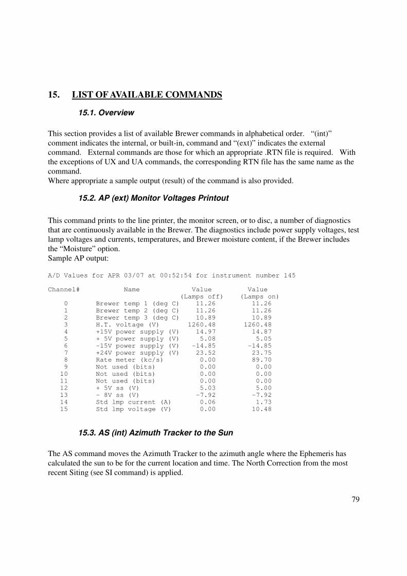
79
15. LIST OF AVAILABLE COMMANDS
15.1. Overview
This section provides a list of available Brewer commands in alphabetical order. “(int)”
comment indicates the internal, or built-in, command and “(ext)” indicates the external command. External commands are those for which an appropriate .RTN file is required. With
the exceptions of UX and UA commands, the corresponding RTN file has the same name as the
command.
Where appropriate a sample output (result) of the command is also provided.
15.2. AP (ext) Monitor Voltages Printout
This command prints to the line printer, the monitor screen, or to disc, a number of diagnostics
that are continuously available in the Brewer. The diagnostics include power supply voltages, test lamp voltages and currents, temperatures, and Brewer moisture content, if the Brewer includes
the “Moisture” option.
Sample AP output:
A/D Values for APR 03/07 at 00:52:54 for instrument number 145 Channel# Name Value Value (Lamps off) (Lamps on) 0 Brewer temp 1 (deg C) 11.26 11.26 1 Brewer temp 2 (deg C) 11.26 11.26 2 Brewer temp 3 (deg C) 10.89 10.89 3 H.T. voltage (V) 1260.48 1260.48 4 +15V power supply (V) 14.97 14.87 5 + 5V power supply (V) 5.08 5.05 6 -15V power supply (V) -14.85 -14.85 7 +24V power supply (V) 23.52 23.75 8 Rate meter (kc/s) 0.00 89.70 9 Not used (bits) 0.00 0.00 10 Not used (bits) 0.00 0.00 11 Not used (bits) 0.00 0.00 12 + 5V ss (V) 5.03 5.00 13 - 8V ss (V) -7.92 -7.92 14 Std lmp current (A) 0.06 1.73 15 Std lmp voltage (V) 0.00 10.48
15.3. AS (int) Azimuth Tracker to the Sun
The AS command moves the Azimuth Tracker to the azimuth angle where the Ephemeris has
calculated the sun to be for the current location and time. The North Correction from the most
recent Siting (see SI command) is applied.
80
15.4. AU (ext) Automatic Operation
The AU command results in the Brewer executing a series of commands which are imbedded the
AU routine (HP HG DS ZS DS ZS DS ZS B1 UV (or UX)). The sequence continues until
interrupted by an operator, or until the sun reaches ZA = 85. At ZA = 85, the system executes the
ED command.
15.5. AZ (ext) Azimuth Tracker Zeroing
The AZ command causes the Azimuth Tracker to return to its zero reference (North) position, and then move the Brewer to the solar azimuth as calculated by the Ephemeris according to the
Location, the Time, and the current North Correction, as determined by the most recent Siting
(see SI command).
15.6. B0 (int) Turn off Lamps
B0 ensures that the Standard Lamp and Mercury Lamps are both off.
15.7. B1 (int) Mercury Lamp ON
B1 turns on the internal Mercury Calibration Lamp, and is useful in a command sequence (i.e.
B1DSHG) where a DS measurement is taken while the Mercury lamp is warming up B1. Note
that if the HG does not execute for some reason, the lamp may be left on and should be turned off
with the B0 command.
15.8. B2 (int) Standard Lamp ON
B2 turns on the internal Standard test Lamp and is useful in a command sequence (i.e. B2ZSSL)
where the ZS measurement is taken while the Standard Lamp is warming up. Note that if the SL
does not execute for some reason, the Lamp may be left on and should be turned off with the B0
command.
15.9. CF (ext) Instrument Constants File Update
CF accesses the Brewer’s Instrument Constants File and allows the operator to make changes. Note that the constants in this file affect the operation and calibration of the instrument, and
normally are not changed unless the instrument is undergoing recalibration or has undergone
81
repairs. This command requires operator input, and changes should be made or approved only by
qualified personnel.
15.10. CI (int) Lamp Scan on Slit #1
CI is used to perform a wavelength scan from 286.5 nm to 366 nm on one of the two internal test
lamps. Filter Wheels are set to positions 1 and 0, and the Iris is open. The increment of the scan
is user selectable with choices of 1, 2, or 5 Angstrom. Data can be compared with the data
contained in the Final Test Record, and is stored in the file CIJJJYY.NNN in the \BDATA
directory. A typical command sequence might be B1W1CI, where B1 turns on the HG lamp, W1
produces a 5-minute lamp warm-up delay, and CI executes the wavelength scan.
15.11. CO (int) Comments
CO allows the operator to enter a comment (up to 75 characters) into the Brewer data file. This
command is useful to record information about a measurement, current weather, sky conditions,
and so on. This command requires operator input. CS (ext) Command Sequence CS is similar
to a command line entry at the cm->__ prompt. The operator may enter a sequence of commands
to be executed, followed by an integer which indicates the number of times the sequence is to be repeated. This command requires operator input.
15.12. CY (int) Slitmask Cycles
The default value for slitmask cycling for most observations is 20. The CY command may be
used to increase or decrease this number if better statistics, or a faster measurement (with
degraded statistics) is desired. This command requires operator input.
15.13. CZ (ext) Custom Scan
CZ allows the operator to define a custom scan. Sources may be one of the internal lamps, the
UV port, or the quartz window. The scan may be over any wavelength range within the Brewer’s UV scan limits, have any wavelength increment, and use any filterwheel combination.
15.14. DA (int) Date Set
The Brewer ephemeris requires GMT (both date and time) for proper operation. Under normal, uninterrupted operation, the computer, and Brewer, dates will change at 00:00:00 UT, and are
displayed on the monitor screen. Under some conditions (power failure at 00:00:00 UT), the date
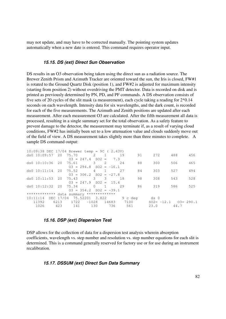
82
may not update, and may have to be corrected manually. The pointing system updates
automatically when a new date is entered. This command requires operator input.
15.15. DS (ext) Direct Sun Observation
DS results in an O3 observation being taken using the direct sun as a radiation source. The
Brewer Zenith Prism and Azimuth Tracker are oriented toward the sun, the Iris is closed, FW#1 is rotated to the Ground Quartz Disk (position 1), and FW#2 is adjusted for maximum intensity
(starting from position 2) without overdriving the PMT detector. Data is recorded on disk and is
printed as previously determined by PN, PD, and PF commands. A DS observation consists of
five sets of 20 cycles of the slit mask (a measurement), each cycle taking a reading for 2*0.14
seconds on each wavelength. Intensity data for six wavelengths, and the dark count, is recorded
for each of the five measurements. The Azimuth and Zenith positions are updated after each
measurement. After each measurement O3 are calculated. After the fifth measurement all data is processed, resulting in a single summary set for the total observation. As a safety feature to
prevent damage to the detector, the measurement may terminate if, as a result of varying cloud
conditions, FW#2 has initially been set to a low attenuation value and clouds suddenly move out
of the field of view. A DS measurement takes slightly more than three minutes to complete. A
sample DS command output:
10:09:38 DEC 17/04 Brewer temp = 9C ( 2.43V) ds0 10:09:57 20 75.70 2 1 19 91 272 488 456 O3 = 247.4 SO2 = 7.3 ds0 10:10:36 20 75.61 3 2 24 88 300 506 465 O3 = 294.8 SO2 = -16.1 ds0 10:11:14 20 75.52 4 1 27 84 303 527 494 O3 = 306.2 SO2 = -27.8 ds0 10:11:53 20 75.43 3 3 18 98 308 543 528 O3 = 247.9 SO2 = 15.4 ds0 10:12:32 20 75.34 0 1 29 86 319 586 525 O3 = 354.2 SO2 = -39.1 ************* data summary ************* 10:11:14 DEC 17/04 75.52201 3.822 9 c deg ds 0 11392 6213 1722 -1028 14683 7100 SO2= -12.1 O3= 290.1 1026 423 141 130 736 561 23.0 44.7
15.16. DSP (ext) Dispersion Test
DSP allows for the collection of data for a dispersion test analysis wherein absorption
coefficients, wavelength vs. step number and resolution vs. step number equations for each slit is
determined. This is a command generally reserved for factory use or for use during an instrument
recalibration.
15.17. DSSUM (ext) Direct Sun Data Summary
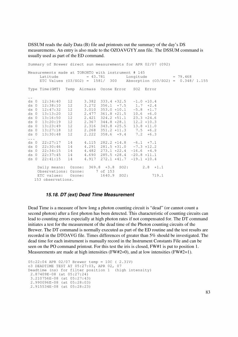
83
DSSUM reads the daily Data (B) file and printouts out the summary of the day’s DS
measurements. An entry is also made to the OZOAVGYY.nnn file. The DSSUM command is usually used as part of the ED command. Summary of Brewer direct sun measurements for APR 02/07 (092) Measurements made at TORONTO with instrument # 145 Latitude = 43.781 Longitude = 79.468 ETC Values (O3/SO2) = 1581/ 300 Absorption (O3/SO2) = 0.348/ 1.155 Type Time(GMT) Temp Airmass Ozone Error SO2 Error …. ds 0 12:34:40 12 3.382 333.4 +32.5 -1.0 +10.4 ds 0 12:38:10 12 3.272 356.1 +7.5 1.7 +2.4 ds 0 12:47:32 12 3.010 353.0 +10.1 -5.8 +1.7 ds 0 13:13:20 12 2.477 361.8 +21.5 10.6 +6.0 ds 0 13:16:50 12 2.421 324.2 +51.1 23.3 +24.6 ds 0 13:20:19 12 2.367 344.8 +28.1 12.2 +10.3 ds 0 13:23:49 12 2.316 343.8 +25.5 13.8 +11.0 ds 0 13:27:18 12 2.268 351.2 +11.3 7.5 +6.2 ds 0 13:30:48 12 2.222 358.6 +9.4 7.2 +6.3 ….. ds 0 22:27:17 14 4.115 282.2 +14.8 -6.1 +7.1 ds 0 22:30:46 14 4.291 281.5 +31.0 -7.3 +12.2 ds 0 22:34:15 14 4.482 273.1 +22.4 -16.6 +4.9 ds 0 22:37:45 14 4.690 285.5 +28.4 -20.8 +11.1 ds 0 22:41:15 14 4.917 272.1 +41.7 -19.1 +10.4 Daily means: Ozone: 369.8 +3.8 SO2: 2.8 +1.1 Observations: Ozone: 7 of 153 ETC values: Ozone: 1640.9 SO2: 719.1
153 observations.
15.18. DT (ext) Dead Time Measurement
Dead Time is a measure of how long a photon counting circuit is “dead” (or cannot count a
second photon) after a first photon has been detected. This characteristic of counting circuits can lead to counting errors especially at high photon rates if not compensated for. The DT command
initiates a test for the measurement of the dead time of the Photon counting circuits of the
Brewer. The DT command is normally executed as part of the ED routine and the test results are
recorded in the DTOAVG file. Times differences of greater than 5% should be investigated. The
dead time for each instrument is manually record in the Instrument Constants File and can be
seen on the PO command printout. For this test the iris is closed, FW#1 is put to position 1.
Measurements are made at high intensities (FW#2=0), and at low intensities (FW#2=1). 05:22:04 APR 02/07 Brewer temp = 10C ( 2.31V) o3 DEADTIME TEST AT 05:27:03, APR 02, 07 Deadtime (ns) for filter position 1 (high intensity) 2.87409E-08 (at 05:27:24) 3.210756E-08 (at 05:27:43) 2.990096E-08 (at 05:28:03) 2.915534E-08 (at 05:28:23)
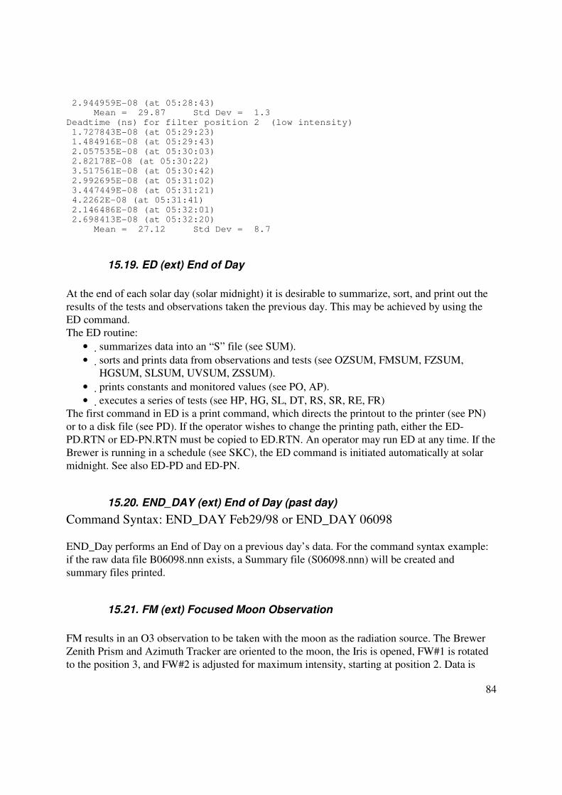
84
2.944959E-08 (at 05:28:43) Mean = 29.87 Std Dev = 1.3 Deadtime (ns) for filter position 2 (low intensity) 1.727843E-08 (at 05:29:23) 1.484916E-08 (at 05:29:43) 2.057535E-08 (at 05:30:03) 2.82178E-08 (at 05:30:22) 3.517561E-08 (at 05:30:42) 2.992695E-08 (at 05:31:02) 3.447449E-08 (at 05:31:21) 4.2262E-08 (at 05:31:41) 2.146486E-08 (at 05:32:01) 2.698413E-08 (at 05:32:20) Mean = 27.12 Std Dev = 8.7
15.19. ED (ext) End of Day
At the end of each solar day (solar midnight) it is desirable to summarize, sort, and print out the
results of the tests and observations taken the previous day. This may be achieved by using the
ED command.
The ED routine:
• summarizes data into an “S” file (see SUM).
• sorts and prints data from observations and tests (see OZSUM, FMSUM, FZSUM,
HGSUM, SLSUM, UVSUM, ZSSUM).
• prints constants and monitored values (see PO, AP).
• executes a series of tests (see HP, HG, SL, DT, RS, SR, RE, FR)
The first command in ED is a print command, which directs the printout to the printer (see PN)
or to a disk file (see PD). If the operator wishes to change the printing path, either the ED-
PD.RTN or ED-PN.RTN must be copied to ED.RTN. An operator may run ED at any time. If the
Brewer is running in a schedule (see SKC), the ED command is initiated automatically at solar
midnight. See also ED-PD and ED-PN.
15.20. END_DAY (ext) End of Day (past day)
Command Syntax: END_DAY Feb29/98 or END_DAY 06098
END_Day performs an End of Day on a previous day’s data. For the command syntax example:
if the raw data file B06098.nnn exists, a Summary file (S06098.nnn) will be created and
summary files printed.
15.21. FM (ext) Focused Moon Observation
FM results in an O3 observation to be taken with the moon as the radiation source. The Brewer
Zenith Prism and Azimuth Tracker are oriented to the moon, the Iris is opened, FW#1 is rotated
to the position 3, and FW#2 is adjusted for maximum intensity, starting at position 2. Data is
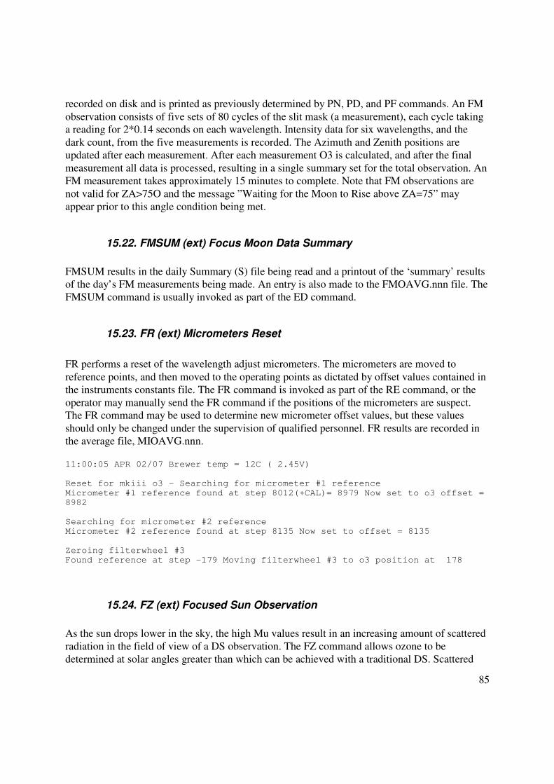
85
recorded on disk and is printed as previously determined by PN, PD, and PF commands. An FM
observation consists of five sets of 80 cycles of the slit mask (a measurement), each cycle taking a reading for 2*0.14 seconds on each wavelength. Intensity data for six wavelengths, and the
dark count, from the five measurements is recorded. The Azimuth and Zenith positions are
updated after each measurement. After each measurement O3 is calculated, and after the final
measurement all data is processed, resulting in a single summary set for the total observation. An
FM measurement takes approximately 15 minutes to complete. Note that FM observations are
not valid for ZA>75O and the message ”Waiting for the Moon to Rise above ZA=75” may
appear prior to this angle condition being met.
15.22. FMSUM (ext) Focus Moon Data Summary
FMSUM results in the daily Summary (S) file being read and a printout of the ‘summary’ results
of the day’s FM measurements being made. An entry is also made to the FMOAVG.nnn file. The FMSUM command is usually invoked as part of the ED command.
15.23. FR (ext) Micrometers Reset
FR performs a reset of the wavelength adjust micrometers. The micrometers are moved to
reference points, and then moved to the operating points as dictated by offset values contained in
the instruments constants file. The FR command is invoked as part of the RE command, or the
operator may manually send the FR command if the positions of the micrometers are suspect. The FR command may be used to determine new micrometer offset values, but these values
should only be changed under the supervision of qualified personnel. FR results are recorded in
the average file, MIOAVG.nnn. 11:00:05 APR 02/07 Brewer temp = 12C ( 2.45V) Reset for mkiii o3 - Searching for micrometer #1 reference Micrometer #1 reference found at step 8012(+CAL)= 8979 Now set to o3 offset = 8982 Searching for micrometer #2 reference Micrometer #2 reference found at step 8135 Now set to offset = 8135 Zeroing filterwheel #3 Found reference at step -179 Moving filterwheel #3 to o3 position at 178
15.24. FZ (ext) Focused Sun Observation
As the sun drops lower in the sky, the high Mu values result in an increasing amount of scattered
radiation in the field of view of a DS observation. The FZ command allows ozone to be
determined at solar angles greater than which can be achieved with a traditional DS. Scattered

86
radiation is measured by offsetting the solar image by 1 degree from the entrance slit, and
observing radiation in the vicinity of the solar disk. This scattered radiation is then subtracted from the direct sun result to give a more accurate measure of the direct radiation, before the
Ozone determination is made. This method will give reasonably accurate O3 values to ZA of
85O (Air Mass =8.2) as compared to the DS which has cut-off angles of 70 to 80O (Air Mass 3.2
to 5) without corrections. This is a useful command at high latitudes and is normally not used
where DS readings are available. For the FZ measurement the iris is closed, FW#1 is set to
position 3, and FW#2 is set to position 5. The minimum zenith angle at which an FZ may be
taken is 73 degrees. See also DS command.
15.25. FZSUM (ext) Focused Sun Data Summary
FZSUM command reads the daily Data (B) file and printouts out the ‘summary’ results of the
day’s FZ measurements. The FZSUM command is usually invoked as part of the ED command.
15.26. GS (ext) Gratings Data Collection
GS initiates a routine that collects data required to calculate Grating Slope and Grating Intercept
values, which ensure that the two gratings are synchronized during scanning. The routine
performs a scan on slits 1 through 5. Data is written to a GSJJJYY.nnn file, and can be processed
by the RD_GS.EXE program to calculate the Grating Slop and Grating Intercept to ensure that
the two gratings are synchronized during scanning operations. GS and RD_GS.EXE are normally run by as part of factory set-up operations or when problems are experienced with the
micrometers or gratings.
15.27. HG (ext) Mercury Wavelength Calibration
HG is used to accurately locate the 302.15 nm line of the Mercury spectrum, and then adjust the
diffraction grating such that the five ozone operational wavelengths fall onto the appropriate exit
slits. The zenith prism rotates to the test lamps (position 0), the iris is opened, FW#1 is rotated to the quartz disk (position 1), FW#2 to ND=0 (position 0). Following the initial set-up and lamp
warm-up, the grating is scanned in the forward and reverse direction and the resulting combined
spectrum is compared to a stored spectrum. Corrections to the micrometer position are made, and
if the adjustment required is greater than 2 steps (.012nm) then the scan is repeated. A test for the
presence of Hg lamp radiation is made prior to the beginning of the scan, and if it is not there, an
FR test is done to reposition the micrometers to pre-set initialization values and the test is redone. Using wide slit0 on line 296.7 nm HG line ... **** HG Calibration **** 05:57:19 APR 02/07 Brewer temp = 11C ( 2.35V) 05:58:58 ( 0.9984 ) corr est for step 971.05 target is step 967 18149 405.96 micro is moved by 4 steps
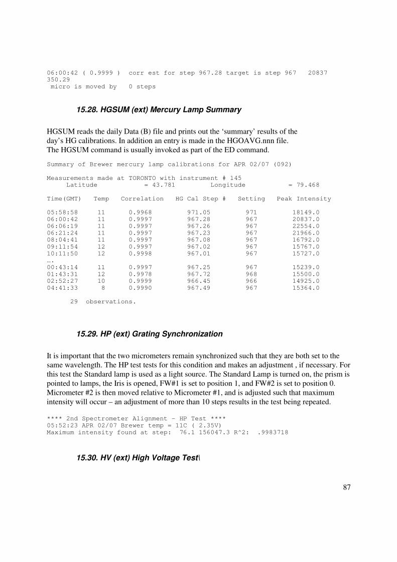
87
06:00:42 ( 0.9999 ) corr est for step 967.28 target is step 967 20837 350.29 micro is moved by 0 steps
15.28. HGSUM (ext) Mercury Lamp Summary
HGSUM reads the daily Data (B) file and prints out the ‘summary’ results of the
day’s HG calibrations. In addition an entry is made in the HGOAVG.nnn file.
The HGSUM command is usually invoked as part of the ED command. Summary of Brewer mercury lamp calibrations for APR 02/07 (092) Measurements made at TORONTO with instrument # 145 Latitude = 43.781 Longitude = 79.468 Time(GMT) Temp Correlation HG Cal Step # Setting Peak Intensity 05:58:58 11 0.9968 971.05 971 18149.0 06:00:42 11 0.9997 967.28 967 20837.0 06:06:19 11 0.9997 967.26 967 22554.0 06:21:24 11 0.9997 967.23 967 21966.0 08:04:41 11 0.9997 967.08 967 16792.0 09:11:54 12 0.9997 967.02 967 15767.0 10:11:50 12 0.9998 967.01 967 15727.0 …. 00:43:14 11 0.9997 967.25 967 15239.0 01:43:31 12 0.9978 967.72 968 15500.0 02:52:27 10 0.9999 966.45 966 14925.0 04:41:33 8 0.9990 967.49 967 15364.0 29 observations.
15.29. HP (ext) Grating Synchronization
It is important that the two micrometers remain synchronized such that they are both set to the same wavelength. The HP test tests for this condition and makes an adjustment , if necessary. For
this test the Standard lamp is used as a light source. The Standard Lamp is turned on, the prism is
pointed to lamps, the Iris is opened, FW#1 is set to position 1, and FW#2 is set to position 0.
Micrometer #2 is then moved relative to Micrometer #1, and is adjusted such that maximum
intensity will occur – an adjustment of more than 10 steps results in the test being repeated.
**** 2nd Spectrometer Alignment - HP Test **** 05:52:23 APR 02/07 Brewer temp = 11C ( 2.35V) Maximum intensity found at step: 76.1 156047.3 R^2: .9983718
15.30. HV (ext) High Voltage Test\
88
The HV command invokes a test used to determine the optimum high voltage setting for the
photomultiplier. The HVSET command can then be used to set the High Voltage. This test is normally used in the factory during the final set-up stages of manufacture, or in the field if it is
suspected that the setting is not correct . The Standard Lamp is turned on, the iris is opened,
FW#1 is put to position 1, and FW#2 is set to position 0. See the HVSET command, and
Appendix F for more details on the HV test.
15.31. HVSET (ext) High Voltage Set-up
The HVSET command can be used to adjust for the optimum High Voltage as determined be the
HV test.
15.32. IC (ext) Instrument Configuration File Update
The IC command results in a display of the Instrument’s current configuration and allows changes to be made by the operator.
15.33. LF (ext) Location File Update
The LF command displays a list of some of the known locations of Brewer sites throughout the world. The geographical co-ordinates of the current site may be entered and/or modified.
15.34. LL (ext) Location Update
The LL command allows an operator to change the co-ordinates of a Brewer location, or for the selection of another site contained the location file.
15.35. NO (ext) Change Instrument
The NO command allows the instrument number of the Brewer to be changed. Each Brewer has
a set of files which are stored in the C:\BDATA\NNN subdirectory, and which are necessary for
proper operation of Brewer NNN. When the NO command is issued, the software is made aware
of which Brewer is connected.
15.36. OZSUM (ext) Ozone Summary
89
OZSUM reads the daily Date (B) file and prints out the summary results of the day’s O3
observations. In addition an entry is made in the OZOAVGYY.nnn file. The OZSUM command is usually invoked as part of the ED command.
Summary of Brewer ozone measurements for DEC 17/04 (352) Measurements made at Punta Arenas with instrument # 017 Latitude = -53.137 Longitude = 70.88 ETC Values (O3/SO2) = 3350/ 3300 Absorption (O3/SO2) = .34110/ 1.1444 Type Time(GMT) Temp Airmass dsO3 zsO3 Error dsSO2 zsSO2 Error zs 0 09:57:15 9 4.339 323.0 +0.8 -44.7 +1.6 zs 0 10:03:53 9 4.079 318.6 +1.0 -35.6 +1.9 ds 0 10:07:57 9 3.933 239.5 +39.6 2.5 +20.7 ds 0 10:11:14 9 3.822 287.6 +44.7 -11.2 +23.0 ds 0 10:16:38 9 3.652 233.3 +50.9 3.4 +11.5 ds 0 10:21:52 9 3.500 319.6 +32.3 -5.2 +9.5 zs 1 15:53:19 17 1.165 290.8 +4.5 10.0 +1.1 ds 0 15:57:28 18 1.163 294.7 +16.8 3.7 +4.9 ds 0 16:00:13 18 1.161 281.3 +46.7 6.2 +9.2 ds 0 16:08:44 18 1.157 248.1 +79.0 11.0 +17.9 ds 0 16:12:09 18 1.155 280.5 +22.4 7.1 +7.6 ds 2 16:17:40 18 1.154 291.6 +15.8 1.7 +3.5 ds 3 16:21:02 18 1.153 303.8 +1.6 -0.7 +0.4 zs 1 16:25:09 18 1.151 291.1 +2.8 10.1 +0.5 ds 2 19:50:45 22 1.447 300.7 +1.0 -1.9 +0.2 ds 3 19:54:06 22 1.460 292.4 +1.4 0.1 +0.2 ds 3 20:08:16 22 1.517 296.3 +2.1 -0.6 +0.5 ds 1 20:11:36 22 1.532 288.2 +7.1 0.9 +1.6 ds 0 20:16:39 21 1.554 278.5 +21.1 3.1 +4.7 ds 2 20:20:21 21 1.572 297.6 +3.1 -1.1 +0.6 ds 3 20:23:41 21 1.588 242.6 +73.6 20.9 +27.3 ds 0 22:58:39 18 3.516 292.5 +18.8 -12.7 +16.9 ds 0 23:01:56 18 3.611 284.9 +68.4 -10.6 +40.3 ds 0 23:05:13 18 3.711 253.0 +51.5 13.4 +17.3 ds 0 23:08:33 18 3.817 267.9 +32.1 -0.2 +9.7 ds 0 23:13:48 18 3.997 282.8 +1.7 -2.3 +0.6 zs 0 23:24:03 18 4.395 323.8 +0.8 -48.0 +1.4 Daily means: 296.0 297.5 -0.7 7.2 Standard deviation: 5.8 11.2 0.6 4.2 Number of observations: 29 /153 8 / 14 167 observations.
15.37. PB (ext) Data Playback
Command Syntax: PB BJJJYY. The PB command allows any previous day’s data to be printed using the current temperature coefficients.
15.38. PD (int) Print to Disk
PD directs printing to a “D” file on the data drive rather than to the line printer. See also PN, PF.
90
15.39. PF (int) Printer Off
PF turns off all printing. Raw data continues to be recorded. See also PN, PD.
15.40. PN (int) Printer ON
PN directs printing to the line printer. See also PD, PF.
15.41. PO (ext) Printout Instrument Constants
PO generates a printout of the instrument constants file. An example of PO output Values:
MKIII BREWER INSTRUMENT #145 ---------------------------- 04-02-2007 11:00:04 ****************************************************************************** * Ozone Values * 1 * 2 * 3 * 4 * 5 * hg * ****************************************************************************** Wavelength(nm) * 306.290 310.029 313.479 316.763 319.958 303.198 Temp. Coeff * 0.0000 -0.7458 -1.3065 -1.4900 -1.8563 0.0000 Disp. Coeff #1 * 2845.570 2885.260 2922.020 2957.400 2991.690 2812.390 Disp. Coeff #2 * 0.081125 0.080329 0.079543 0.078609 0.077790 0.081985 Disp. Coeff #3 *-0.701E-6 -0.716E-6 -0.730E-6 -0.727E-6 -0.740E-6 -0.715E-6 ****************************************************************************** ETC Values : O3 = 1581 ; SO2 = 300 O3 Absn Coeffs : O3 = 0.3476 ; SO2 = 1.1550 SO2 Absn Coeffs : O3 = 0 ; SO2 = 2.3500 Micrometer steps/deg = 0.00 WL cal step number = 967 Micrometer Zero = 1777 Umkehr offset = 2282 Iris Open Steps = 250 Zenith steps/rev = 2816 Slit mask motor delay = 96 Micrometer 1 Offset O3 = 8982 Micrometer 2 Offset = 8135 Grating Slope = 1 Grating Intercept = -8 Filterwheel 3 Offset O3 = 178 Dead Time(ns) = 32 Zenith Offset = 23 Buffer Delay(s) = 0.2 Zenith UVB Dome Position = 2091 Note: Faster Processors May Require a Longer Buffer Delay (Typically 0.2 to 0.8 Seconds)
15.42. PZ (int) Point to Zenith
PZ results in the Zenith Prism being pointed to a Zenith angle of 0 (straight upwards).
91
15.43. QS (ext) Quick Scan
QS is used in conjunction with the UV Stability Check Kit, and gives an indication of the
stability of the instrument in the intensity measurement of UV over the range 290nm to 325nm.
When the equipment has been set up as per the instructions in Section of this manual, and the QS
command issued, a report is generated which shows the stability of the instrument at 3.5nm increments using the first generated set of readings as a reference. For the test, the iris is opened,
FW#1 is set to position 3, and FW#2 is set to position 1.
15.44. RE (ext) Reset
RE initializes all of the Brewer motors (similar to the Power On initialisation), and moves them
to positions as defined in the Instruments Constants File. Following a RE, the iris is closed,
FW#1 is in position 1, and FW#2 is in position 3. Zenith diode found at :-21 Zenith zeroed at 05:42:20 Zenith discrepancy = -2 -10509 2931 13448 Azimuth diode found at : 13440 Azimuth zeroed at 05:44:02 Azimuth discrepancy = 8 Trying to zero filterwheel #3 Found diode at step -177 Moving filterwheel #3 to o3 position at 178 05:44:33 APR 02/07 Brewer temp = 11C ( 2.35V) Reset for mkiii o3 - Searching for micrometer #1 reference Micrometer #1 reference found at step 8008(+CAL)= 8975 Now set to o3 offset = 8982 Searching for micrometer #2 reference Micrometer #2 reference found at step 8133 Now set to offset = 8135 Zeroing filterwheel #3 Found reference at step -179 Moving filterwheel #3 to o3 position at 178
15.45. REP (ext) Report
REP displays (or prints) the SLOAVG, HGOAVG, APOAVG, DTOAVG, MIOAVG, and
RSOAVG over a user selected range of days.
15.46. RS (ext) Slit Mask Run/Stop Test
A malfunction in the slit mask motor circuit or in the slit mask itself can result in improper
counting and consequently incorrect data. The RS test produces a report on the operation of the
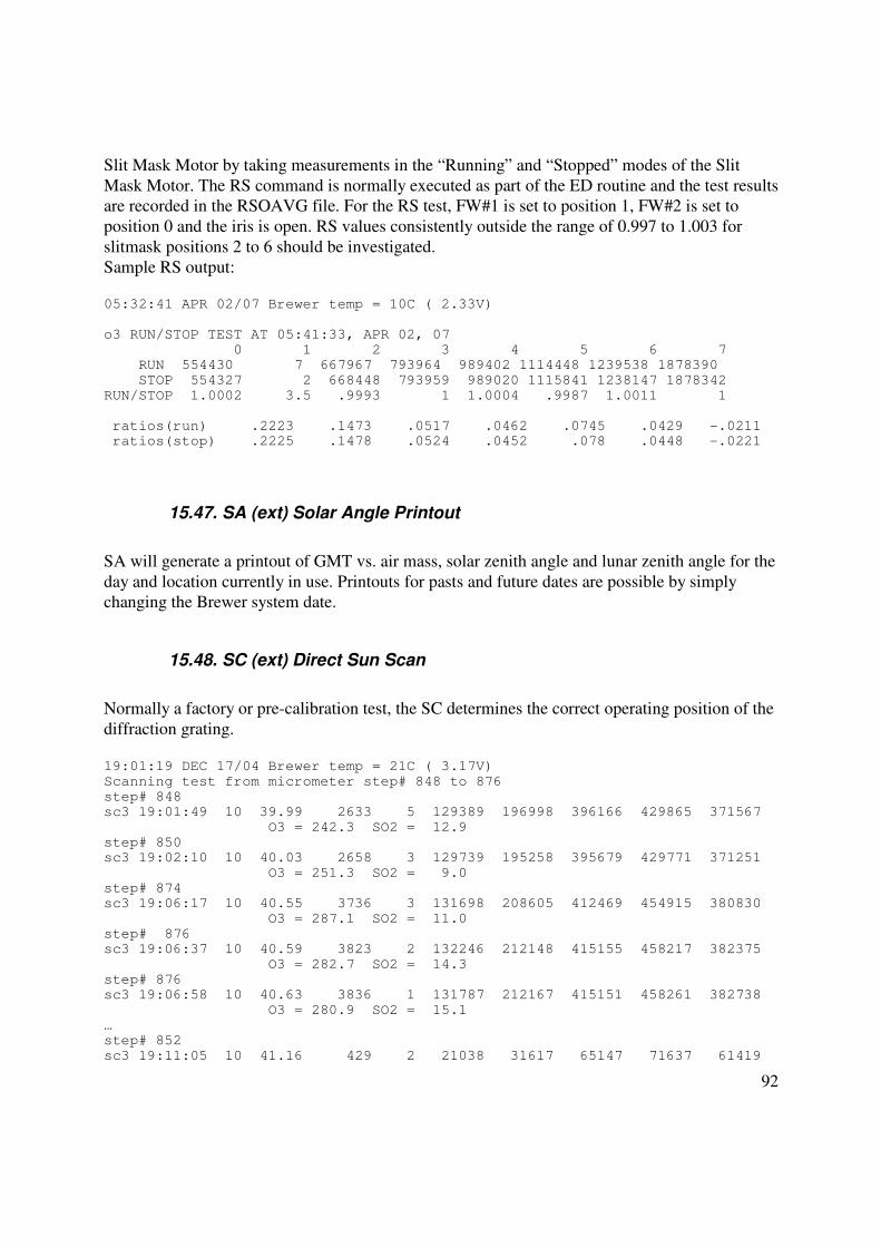
92
Slit Mask Motor by taking measurements in the “Running” and “Stopped” modes of the Slit
Mask Motor. The RS command is normally executed as part of the ED routine and the test results are recorded in the RSOAVG file. For the RS test, FW#1 is set to position 1, FW#2 is set to
position 0 and the iris is open. RS values consistently outside the range of 0.997 to 1.003 for
slitmask positions 2 to 6 should be investigated.
Sample RS output: 05:32:41 APR 02/07 Brewer temp = 10C ( 2.33V) o3 RUN/STOP TEST AT 05:41:33, APR 02, 07 0 1 2 3 4 5 6 7 RUN 554430 7 667967 793964 989402 1114448 1239538 1878390 STOP 554327 2 668448 793959 989020 1115841 1238147 1878342 RUN/STOP 1.0002 3.5 .9993 1 1.0004 .9987 1.0011 1 ratios(run) .2223 .1473 .0517 .0462 .0745 .0429 -.0211 ratios(stop) .2225 .1478 .0524 .0452 .078 .0448 -.0221
15.47. SA (ext) Solar Angle Printout
SA will generate a printout of GMT vs. air mass, solar zenith angle and lunar zenith angle for the
day and location currently in use. Printouts for pasts and future dates are possible by simply changing the Brewer system date.
15.48. SC (ext) Direct Sun Scan
Normally a factory or pre-calibration test, the SC determines the correct operating position of the
diffraction grating.
19:01:19 DEC 17/04 Brewer temp = 21C ( 3.17V) Scanning test from micrometer step# 848 to 876 step# 848 sc3 19:01:49 10 39.99 2633 5 129389 196998 396166 429865 371567 O3 = 242.3 SO2 = 12.9 step# 850 sc3 19:02:10 10 40.03 2658 3 129739 195258 395679 429771 371251 O3 = 251.3 SO2 = 9.0 step# 874 sc3 19:06:17 10 40.55 3736 3 131698 208605 412469 454915 380830 O3 = 287.1 SO2 = 11.0 step# 876 sc3 19:06:37 10 40.59 3823 2 132246 212148 415155 458217 382375 O3 = 282.7 SO2 = 14.3 step# 876 sc3 19:06:58 10 40.63 3836 1 131787 212167 415151 458261 382738 O3 = 280.9 SO2 = 15.1 … step# 852 sc3 19:11:05 10 41.16 429 2 21038 31617 65147 71637 61419

93
O3 = 262.6 SO2 = 5.0 step# 850 sc3 19:11:26 10 41.20 5 2 90 122 253 290 249 O3 = 293.2 SO2 = -13.0 step# 848 sc3 19:11:46 10 41.24 6 3 48 90 151 173 134 O3 = 269.8 SO2 = 53.4
15.49. SE (ext) Schedule Edit
SE is used to create or modify Brewer operating schedules, which are stored as “.SKD” files in
the Brewer directory. Brewer schedules consist of two columns of data - a solar zenith angle, and
a string of commands. The string of commands is executed at the corresponding solar zenith
angle. The SA command is useful for converting GMT to solar angle. See also the SK and SKC
commands.
15.50. SH (ext) Slit Mask (shutter) Motor Timing Test
Normally a factory test, the SH command is used to determine the timing constant used in the
control of the slit mask motor.
DELAY CAL DARK WAVELENGTH 1 10 1737768 7557 92828 12 1738031 480 93450 14 1737408 39 93100 16 1738864 37 93422 18 1738388 44 93318 20 1737191 28 93579 22 1738692 36 93580 24 1742088 40 93713 26 1737650 34 93666 28 1737937 32 93596 30 1739330 35 93605 32 1738615 41 93749 34 1738849 33 94036 36 1737947 35 93859 38 1738791 34 94128 40 1738398 39 93948 42 1710601 43 94193 44 1738853 41 94077 46 1737273 42 94555 48 1737608 44 94805 50 1735986 41 95543
15.51. SI (ext) Solar Siting
Brewer observations using the solar disc as the radiation source require that the Zenith Prism of
the instrument be pointed very accurately toward the sun. The SI command is used in the initial
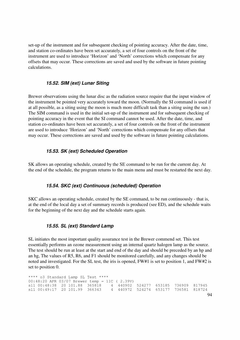
94
set-up of the instrument and for subsequent checking of pointing accuracy. After the date, time,
and station co-ordinates have been set accurately, a set of four controls on the front of the instrument are used to introduce ‘Horizon’ and ‘North’ corrections which compensate for any
offsets that may occur. These corrections are saved and used by the software in future pointing
calculations.
15.52. SIM (ext) Lunar Siting
Brewer observations using the lunar disc as the radiation source require that the input window of
the instrument be pointed very accurately toward the moon. (Normally the SI command is used if
at all possible, as a siting using the moon is much more difficult task than a siting using the sun.) The SIM command is used in the initial set-up of the instrument and for subsequent checking of
pointing accuracy in the event that the SI command cannot be used. After the date, time, and
station co-ordinates have been set accurately, a set of four controls on the front of the instrument
are used to introduce ‘Horizon’ and ‘North’ corrections which compensate for any offsets that
may occur. These corrections are saved and used by the software in future pointing calculations.
15.53. SK (ext) Scheduled Operation
SK allows an operating schedule, created by the SE command to be run for the current day. At
the end of the schedule, the program returns to the main menu and must be restarted the next day.
15.54. SKC (ext) Continuous (scheduled) Operation
SKC allows an operating schedule, created by the SE command, to be run continuously - that is,
at the end of the local day a set of summary records is produced (see ED), and the schedule waits
for the beginning of the next day and the schedule starts again.
15.55. SL (ext) Standard Lamp
SL initiates the most important quality assurance test in the Brewer commend set. This test
essentially performs an ozone measurement using an internal quartz halogen lamp as the source.
The test should be run at least at the start and end of the day and should be preceded by an hp and
an hg, The values of R5, R6, and F1 should be monitored carefully, and any changes should be
noted and investigated. For the SL test, the iris is opened, FW#1 is set to position 1, and FW#2 is set to position 0.
**** o3 Standard Lamp SL Test **** 00:48:20 APR 03/07 Brewer temp = 11C ( 2.39V) sl1 00:48:38 20 101.88 365818 4 440902 524277 653185 736909 817945 sl1 00:49:17 20 101.99 366343 4 440972 524274 653177 736581 818724
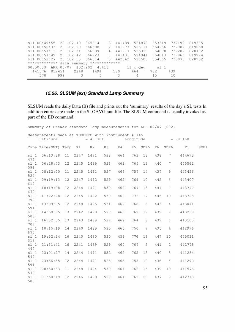
95
sl1 00:49:55 20 102.10 365614 3 441489 524873 653319 737192 819365 sl1 00:50:33 20 102.20 366308 2 441977 525114 654266 737982 819058 sl1 00:51:11 20 102.31 366889 4 441917 525329 654678 737287 820192 sl1 00:51:49 20 102.42 366923 6 441431 524944 654813 737965 819994 sl1 00:52:27 20 102.53 366614 3 442342 526503 654565 738070 820902 ************* data summary ************* 00:50:33 APR 03/07 102.202 4.418 11 c deg sl 1 441576 819454 2248 1494 530 464 762 439 570 999 3 5 3 4 15 10
15.56. SLSUM (ext) Standard Lamp Summary
SLSUM reads the daily Data (B) file and prints out the ‘summary’ results of the day’s SL tests In
addition entries are made in the SLOAVG.nnn file. The SLSUM command is usually invoked as part of the ED command.
Summary of Brewer standard lamp measurements for APR 02/07 (092) Measurements made at TORONTO with instrument # 145 Latitude = 43.781 Longitude = 79.468 Type Time(GMT) Temp R1 R2 R3 R4 R5 SDR5 R6 SDR6 F1 SDF1 sl 1 06:13:38 11 2247 1491 528 464 762 13 438 7 444673 474 sl 1 06:28:43 12 2245 1489 526 462 765 13 440 7 445562 591 sl 1 08:12:00 11 2245 1491 527 465 757 14 437 9 443456 524 sl 1 09:19:13 12 2247 1492 529 462 769 10 442 6 443407 612 sl 1 10:19:08 12 2244 1491 530 462 767 13 441 7 443747 670 sl 1 11:22:28 12 2245 1492 530 460 772 17 445 10 443728 790 sl 1 13:09:05 12 2248 1495 531 462 768 6 443 4 443041 591 sl 1 14:50:35 13 2242 1490 527 463 762 19 439 9 443238 500 sl 1 16:32:55 13 2243 1489 529 462 764 8 439 6 443105 707 sl 1 18:15:19 14 2240 1489 525 465 750 9 435 4 442976 670 sl 1 19:52:34 16 2240 1490 530 458 776 19 447 10 445031 316 sl 1 21:31:41 16 2241 1489 529 460 767 5 441 2 442778 447 sl 1 23:01:27 14 2244 1491 532 462 765 13 440 8 441284 547 sl 1 23:56:35 12 2244 1491 528 465 755 10 436 6 441290 591 sl 1 00:50:33 11 2248 1494 530 464 762 15 439 10 441576 570 sl 1 01:50:49 12 2246 1490 529 464 762 20 437 9 442713 500
96
sl 1 02:59:46 10 2249 1497 528 461 772 18 448 9 442042 689 sl 1 04:48:52 8 2253 1497 531 461 779 15 449 10 442880 670 Daily means: 2245 1492 529 462 765 441 443140 Standard dev: 3 3 2 2 7 4 1188 18 observations.
15.57. SR (ext) Azimuth Tracker Steps Per Revolution
SR initiates a test that determines the number of motor steps required for one complete
revolution (360O) of the Azimuth Tracker. The tracker is first zeroed in the counter clockwise
direction, and a discrepancy between where the software thought it was, and where the zero
reference was found, is output. The Tracker is then moved a full revolution clockwise and the total number of steps required for this movement is output, and the operator is given an
opportunity to save the new value. A progressive change of value over time may suggest that
Tracker maintenance is required.
15.58. SS (ext) Direct Sun UV Scan
SS results in the Brewer performing a UV scan of the sun through the quartz window. The scan is
in 0.5nm steps over the range 290nm to 363nm. Data is stored in a SSJJJYY.nnn file. No response file is available for this mode of UV scanning.
15.59. ST (ext) Status and Control
ST permits the operator to switch the Brewer’s internal lamps off and on, and to control all Brewer stepper motors except the Slit Mask Motor.
15.60. SUM (ext) Summary Data File
SUM reads the daily raw data (BJJJYY.nnn) file and generates a new (SJJJYY.nnn) file which contains only data summary information. In addition, Umkehr data is processed and put into a
separate (UJJJYY.nnn) file. The SUM command, and the various summary printout commands
are generally performed at local midnight as part of the ED command.
15.61. TE (int) Temperature Printout
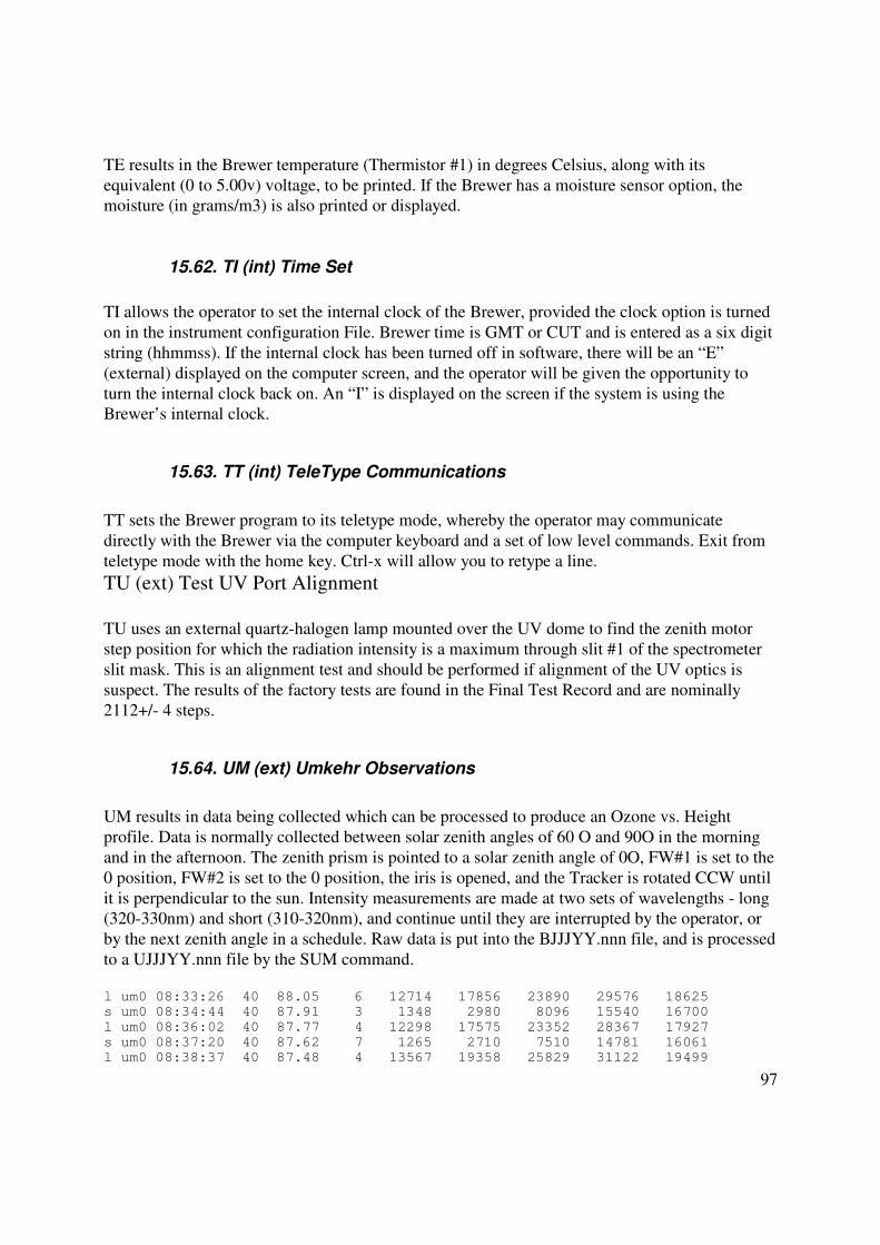
97
TE results in the Brewer temperature (Thermistor #1) in degrees Celsius, along with its
equivalent (0 to 5.00v) voltage, to be printed. If the Brewer has a moisture sensor option, the moisture (in grams/m3) is also printed or displayed.
15.62. TI (int) Time Set
TI allows the operator to set the internal clock of the Brewer, provided the clock option is turned
on in the instrument configuration File. Brewer time is GMT or CUT and is entered as a six digit
string (hhmmss). If the internal clock has been turned off in software, there will be an “E”
(external) displayed on the computer screen, and the operator will be given the opportunity to
turn the internal clock back on. An “I” is displayed on the screen if the system is using the Brewer’s internal clock.
15.63. TT (int) TeleType Communications
TT sets the Brewer program to its teletype mode, whereby the operator may communicate
directly with the Brewer via the computer keyboard and a set of low level commands. Exit from
teletype mode with the home key. Ctrl-x will allow you to retype a line.
TU (ext) Test UV Port Alignment TU uses an external quartz-halogen lamp mounted over the UV dome to find the zenith motor
step position for which the radiation intensity is a maximum through slit #1 of the spectrometer
slit mask. This is an alignment test and should be performed if alignment of the UV optics is
suspect. The results of the factory tests are found in the Final Test Record and are nominally
2112+/- 4 steps.
15.64. UM (ext) Umkehr Observations
UM results in data being collected which can be processed to produce an Ozone vs. Height
profile. Data is normally collected between solar zenith angles of 60 O and 90O in the morning
and in the afternoon. The zenith prism is pointed to a solar zenith angle of 0O, FW#1 is set to the
0 position, FW#2 is set to the 0 position, the iris is opened, and the Tracker is rotated CCW until
it is perpendicular to the sun. Intensity measurements are made at two sets of wavelengths - long (320-330nm) and short (310-320nm), and continue until they are interrupted by the operator, or
by the next zenith angle in a schedule. Raw data is put into the BJJJYY.nnn file, and is processed
to a UJJJYY.nnn file by the SUM command.
l um0 08:33:26 40 88.05 6 12714 17856 23890 29576 18625 s um0 08:34:44 40 87.91 3 1348 2980 8096 15540 16700 l um0 08:36:02 40 87.77 4 12298 17575 23352 28367 17927 s um0 08:37:20 40 87.62 7 1265 2710 7510 14781 16061 l um0 08:38:37 40 87.48 4 13567 19358 25829 31122 19499
98
s um0 08:39:55 40 87.33 6 1531 3455 9841 19713 21268
15.65. UV Related Commands
There are a number of Brewer commands that are related to measurements taken through the
Ultra Violet (UV) Dome, and they are grouped together here for convenience. There are typically
two UV scan lengths - ‘short’ UVB scans, which cover the range from 290nm to 325nm, and
‘extended’ UV scans which cover the range 286.5nm to 363nm.
15.66. UA (ext UV.RTN) Timed UX scan
UA performs an Extended UV scan in 0.5nm increments and stores the data to a UVJJJYY.nnn
file. This is a ‘timed’ routine in that it starts on the next half hour after the command is given. On
execution of the command, the prism is rotated to the UV dome, FW#2 is moved to the 1
position, FW#1 is moved to the 3 position, the iris is opened, and the tracker is pointed at the
sun.
15.67. UB (ext) UV Summary for Schedules
Raw UV scan data is stored in a UVJJJYY.nnn data file. The UB scan instructs the program to
process and print the daily summary for UV measurements taken throughout the day. Damaging
Ultra-Violet values are calculated for each scan and written to a DUVJJJYY.nnn.
15.68. UF Fast UVB scan
UF results in a UV scan being done in the ascending wavelength direction only. The zenith prism
is rotated to the UV dome, FW#2 is set to the 1 position, FW#1 is set to the 3 position, the iris is
opened, and the tracker is pointed to the sun. The UV spectrum is scanned in steps of 0.5nm,
with and integration of 4 shutter cycles for wavelengths less than 300nm, and an integration of 1 shutter cycle for wavelengths grater than 300nm. All data is normalised to a 1 cycle observation
and recorded in a UFJJJYY.nnn data file. When scanning is complete, a calculation of the
UVB/UVA McKinley - Diffey weighted irradiance is computed and sent to the printer and
written to the DUVJJJYY.nnn data file.
15.69. UL (ext) UV Lamp Scan
UL is a test command that results in a UV scan being performed with a Lamp (rather than the sky) being the source of radiation. The zenith prism is rotated to the UV dome, FW#2 is set to
the 1 position, FW#1 is set to the 3 position, the iris is opened, and the tracker is rotated to the
99
sun. The operator is asked for lamp number, and lamp-diffuser separation, and the radiation
intensity is measured in 1.5nm increments over the UVB range. Data is stored in a ULJJJYY.nnn file.
15.70. UV (ext) UV(B) Observation
UV results in the irradiance over the “B” region of the spectrum to be measured. The zenith
prism is rotated to the UV dome, FW#2 is set to the 1 position, FW#1 is set to the 3 position, the
iris is opened, and the tracker is pointed toward the sun. The UV spectrum is then scanned in
steps of 0.5nm from 290nm to 325nm, and then back to 290 nm. The data is appended to a
UVJJJYY.nnn data file. When scanning is complete, a calculation of the UVB/UVA McKinley- Diffey weighted irradiance is computed, sent to the printer and to the monitor screen,
and appended to the DUVJJJYY.nnn data file. A correction is made to the Diffey action
spectrum to include the effects of the UVA region 325-400nm).
15.71. UVSUM (ext) UV Data Summary
This command initiates activity which processes and prints the daily summary of all UV
measurements made during that day. DUV values are also calculated for each measurement and data is appended to the UVOAVG.nnn file.
15.72. UX (ext UV.RTN) Extended UV Wavelength Scan
UX causes the irradiance over the 286.5nm to 363nm range to be measured in 0.5nm increments
in ascending wavelength. The zenith prism is rotated to the UV dome, FW#2 is set to the 1
position, FW#1 is set to the 0 position, the iris is opened, and the tracker is pointed toward the
sun. The UV spectrum is scanned, and the data is appended to a UVJJJYY.nnn data file When scanning is complete, a calculation of the UVB / UVA McKinley- Diffey weighted irradiance is
computed, output to the printer and to the monitor screen, and appended to the DUVJJJYY.nnn
data file.
15.73. W0-W4 (ext) Time delays
These five commands result in time delays of 1, 5, 10, 20, and 30 minutes respectively and can
be used in command strings or in schedules.
15.74. XL (ext) Extended External Lamp Scan
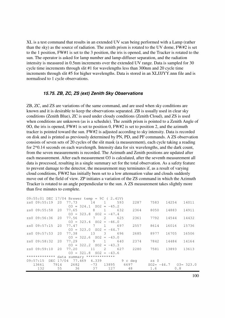
100
XL is a test command that results in an extended UV scan being performed with a Lamp (rather
than the sky) as the source of radiation. The zenith prism is rotated to the UV dome, FW#2 is set to the 1 position, FW#1 is set to the 3 position, the iris is opened, and the Tracker is rotated to the
sun. The operator is asked for lamp number and lamp-diffuser separation, and the radiation
intensity is measured in 0.5nm increments over the extended UV range. Data is sampled for 30
cycle time increments through slit #1 for wavelengths less than 300nm and 20 cycle time
increments through slit #5 for higher wavelengths. Data is stored in an XLJJJYY.nnn file and is
normalised to 1 cycle observations.
15.75. ZB, ZC, ZS (ext) Zenith Sky Observations
ZB, ZC, and ZS are variations of the same command, and are used when sky conditions are
known and it is desirable to keep the observations separated. ZB is usually used in clear sky
conditions (Zenith Blue), ZC is used under cloudy conditions (Zenith Cloud), and ZS is used
when conditions are unknown (as is a schedule). The zenith prism is pointed to a Zenith Angle of
0O, the iris is opened, FW#1 is set to position 0, FW#2 is set to position 2, and the azimuth
tracker is pointed toward the sun. FW#2 is adjusted according to sky intensity. Data is recorded on disk and is printed as previously determined by PN, PD, and PF commands. A ZS observation
consists of seven sets of 20 cycles of the slit mask (a measurement), each cycle taking a reading
for 2*0.14 seconds on each wavelength. Intensity data for six wavelengths, and the dark count,
from the seven measurements is recorded. The Azimuth and Zenith positions are updated after
each measurement. After each measurement O3 is calculated, after the seventh measurement all
data is processed, resulting in a single summary set for the total observation. As a safety feature
to prevent damage to the detector, the measurement may terminates if, as a result of varying cloud conditions, FW#2 has initially been set to a low attenuation value and clouds suddenly
move out of the field of view. ZP initiates a variation of the ZS command in which the Azimuth
Tracker is rotated to an angle perpendicular to the sun. A ZS measurement takes slightly more
than five minutes to complete.
09:55:01 DEC 17/04 Brewer temp = 9C ( 2.41V) zs0 09:55:19 20 77.73 14 1 593 2287 7583 14254 14011 O3 = 324.1 SO2 = -45.2 zs0 09:55:58 20 77.65 8 1 632 2364 8050 14883 14911 O3 = 323.8 SO2 = -47.4 zs0 09:56:36 20 77.56 7 2 625 2361 7792 14544 14432 O3 = 323.4 SO2 = -46.0 zs0 09:57:15 20 77.47 7 1 697 2557 8614 16016 15736 O3 = 323.0 SO2 = -44.7 zs0 09:57:53 20 77.38 13 3 696 2685 8977 16705 16506 O3 = 322.6 SO2 = -43.0 zs0 09:58:32 20 77.29 9 1 640 2374 7842 14484 14164 O3 = 322.2 SO2 = -43.3 zs0 09:59:10 20 77.20 11 2 627 2280 7581 13893 13613 O3 = 321.8 SO2 = -43.6 ************* data summary ************* 09:57:15 DEC 17/04 77.469 4.339 9 c deg zs 0 13661 7914 2682 -73 13895 6697 SO2= -44.7 O3= 323.0 132 55 36 37 127 48 1.6 0.8

101
15.76. ZE (ext) Zero Zenith Prism
ZE positions the zenith prism to its zero-step position, or ZA=180O. The zenith
reference is found, and the prism is then moved back a constant number of steps
from the zero-step position.

102
16. DIAGNOSTIC AND TROUBLESHOOTING PROCEDURES
103
Initial Assembly, Alignment and Test Procedures
16.1. Aligning and focussing a Single Brewer
16.1.1. Preparing for Alignment - Removing the Optical Frame
Equipment Required:
Assorted hand tools. Spacer blocks to support the Brewer optical frame so that it does
not rock on the screw heads and grating supports that protrude under the main plate of the optical
frame.
The Brewer should be removed from the tracker and transported to a suitable clean, dry
location. The cover is removed (see Appendix A.2). The fore-optics of the Brewer are
removed (see Appendix A.2). The cover is taken off the spectrometer housing (see Appendix
A.3). Remove the optical frame from the bulkhead (see Appendix A.4). In the case of the
double Brewer, separate the two halves of the optical frame by removing the three links that join
them (Appendix A.5). The subsequent alignment steps must be done on both of the separated
optical frames. The optical frame can be set down on a table if there are three suitable blocks to put underneath to prevent the grating mount from touching the surface.
16.1.2. Setting up
Equipment Required:
Assorted hand tools. Alignment blocks (3): 1 cm x 2 cm x 6 cm aluminum blocks with
1-mm holes centred on the cm face 5 cm above the base.
If this is a ‘first-time’ alignment, adjust the alignment screws if necessary and appropriate
to have opposite ends of the main mirror the same distance from the slit mounting bulkhead at a distance of approximately 15 cm.
Set up a laser source on the work table and adjust its height so the light hits the centre of
the entrance slit of the Brewer running parallel to the table. Rotate the optical frame to make
this beam run parallel to the edge of the optical frame. Place an alignment block just behind the
tilted correction lens and adjust the laser and optical frame to have the beam go through the hole.
Put a second block in front of the mirror and adjust the laser and optical frame to ensure that the beam goes through the holes in both of the blocks and remains parallel to the side of the optical
frame.
104
16.1.3. Input side alignment.
Equipment Required:
Assorted hand tools. Alignment blocks (3): 1 cm x 2 cm x 6 cm aluminum blocks with 1-mm holes centred on the cm face 5 cm above the base.
Without disturbing the alignment, move the second alignment block from in front of the
mirror and check to see that the beam bouncing from the mirror hits the diffraction grating at the
correct height. This can be done by moving the second alignment block near to the grating and
seeing that the beam clears the hole and strikes the grating near the centre (±2 mm). Exercise extreme care to ensure that neither the block nor any part of the body touches the mirror. If the
test fails, then an adjustment of the main mirror maybe necessary. If the main mirror needs to be
adjusted , re-check the laser with the two alignment blocks to be sure that it is still aligned
properly, and then adjust the top screw of the mirror to bring the beam to the correct height to go
through the hole. The locking screw above the adjusting screw must be loosened slightly before
the adjustment can be made.
16.1.4. Grating rotation.
Equipment Required:
Assorted hand tools. Alignment blocks (3): 1 cm x 2 cm x 6 cm aluminum blocks with
1-mm holes centred on the cm face 5 cm above the base.
Once the incoming beam is hitting the grating at the right point, it is necessary to remove
the push rod and swing the grating. Depending on the diffraction grating used, it is possible to
see at least 3 beams coming from the grating. One is at the specular reflection angle (angle of
incidence equals angle of reflection; sometimes normal to the grating surface depending on the grating angle). With the grating arm at an appropriate angle, the grating tilt adjustment should
be used to put the reflected beam into the correct plane so that it reflects back and goes through
the hole on the first alignment block or through the second alignment block placed on the frame
where it can intersect the mirror reflection from the grating.
The tilt of the grating is adjusted using the top adjustment screw accessed from behind
the grating. It is necessary to loosen the two locking screws (which also secure the pulling springs that load the grating in the tilt direction) before the tilt adjustment can be made.
With the grating in this position, the -1 or +1 order of the grating should be checked with
an alignment block to see that those beams are also in the same plane. If they are not, then the
rotation of the grating lines should be adjusted to bring the +1 and -1orders into the same plane
with the reflected beam.
105
The rotation of the grating is accomplished by rotating the vertical support screws accessed through the grating mounting blocks from underneath the grating. The locking screws
are loosened first and then the two rotating screws are adjusted in opposite directions. Begin
with a 1/4 turn and determine the correct amount needed by watching the motion of the diffracted
beam.
Once the necessary adjustments are complete, re-tighten the three locking screws and re-
check the alignment. Repeat the process as necessary so the beams are centred where they belong to less than 1/5 of the diameter of the alignment block holes (to about 1/5 mm).
With the beams properly aligned up to the point where they leave the diffraction grating, it is
necessary to swing the grating so that the diffracted beam on the exit slit side reflects from near the
centre of the exit side of the main mirror. A small adjustment of the top main mirror adjusting
screw should then be made to cause the beam to hit the exit slits at the horizontal centre-line. (In
the case of the re-combining half of the double instrument, it is necessary to place a paper screen with a centre-line and a reference point at the focus of the spectrometer as a substitute for the slit
plate - include a figure to print to paper to use as the reference plane. Need dimensions for where
to place it.). At this point, a piece of cellotape (frosted) should be placed on the outside surface of
the entrance slit light shield. This will diffuse the laser beam so that the full area of the entrance
slit is filled. The mirror then should be adjusted to centre the image at the exit slits in the vertical
direction.
16.1.5. Focussing.
Equipment Required:
Assorted hand tools. In a properly focussed instrument, rays coming from any part of the
aperture (point on the grating) should wind up at the same point along the length of focal plane.
This can be tested using the laser by sending it into the entrance slit from different angles in the
horizontal plane with no diffuser in place, and using the micrometer to make accurate, relative
position measurements.:
Remove any alignment blocks and re-install the push rod before proceeding with the focussing step. The laser should be moved around in the horizontal plane and the position of the
image of the of the entrance slit on the exit slit plate observed. First the laser position is marked on
the bench with the beam entering along the optical axis of the instrument as in the alignment
procedure above. Then the beam is made to enter the entrance slit at an angle so that the laser spot
hits the grating about 3/4 of the way to the edge of the useful grating surface. This position should
be marked on the bench so it can be repeated. A similar mark is made with the laser entering at an
angle from the other side.
106
16.1.6. Beam along the Optical Axis
Starting with beam along the optical axis (hitting the centre of the main mirror an the grating), adjust the micrometer to position the image of the entrance slit exactly on the edge of one
of the exit slits, preferably the middle one. The most accurate adjustment is to set the beam to be
consistently just beginning to illuminate one side of the exit slit. Record the micrometer reading to
the nearest 1/10 of a division.
16.1.7. Beam entering the right of the Optical Axis
Set the laser up so that the beam enters from the extreme right-hand side as marked in
Step 2. Find the micrometer setting that illuminates the edge of the slit as in Step 3. Record the
setting.
16.1.8. Beam entering the Left of the Optical Axis
Set the laser up so that the beam enters from the extreme left-hand side as marked in
Step 2. Find the micrometer setting that illuminates the edge of the slit as in Step 3. Record the
setting.
16.1.9. Make a Plot
Plot the number recorded in Steps 3 to 5 against left, right and centre. The plot may look like a straight line or a parabola. If it is a fairly symmetrical parabola then the instrument is in goo
focus. Other wise and adjustment is needed. If an adjustment is needed go to Step 7. Otherwise
jump to Step 10.
16.1.10. Adjusting the focus.
The first adjustment will just be a trial to assess the sign of the error and calibrate the sensitivity of
the adjustment. It may go the wrong way and make things worse. For the first adjustment move
both the bottom two mirror screws by ½ turn in the same direction. Subsequently adjust by the
amount estimated in Step 8. Adjust the top screw to vertically centre the image of the entrance slit
on the exit slit centre-line again. (If this step is being done as part of the re-focussing of the
dispersing half of the instrument in the UV, then the half power points must be found by adjusting the top screw each way to half-power and then setting it at the mid-way point before adjusting
anything else. See Appendix A.6 for instructions on how to read out the intensity.)
16.1.11. Repeat the Focus Measurement

107
Repeat steps 3 to 6. Examine the plot. Did the line get steeper or more shallow? By how much.? If it got steeper, the screws were turned the wrong way. Adjust the opposite direction by 1 turn and
repeat 3 to 6. If the curve became shallower compute the change in end-to-end amplitude of the
line and adjust by ½ turn times the remaining amplitude divided by the change in amplitude that
occurred because of the adjustment. (Figures.) Repeat the adjustments until a parabola results
with the left and right end points at approximately the same position.
16.1.12. Re-assembly
Perform the operations in Appendix A.5 in reverse order.
16.1.13. UV Focus
Because the spectrometer focus is slightly different in the visible and the UV, once the laser
alignment is done, the focussing steps (steps 5 to 11) must be repeated once the spectrometer and
fore-optics are replaced in the instrument. The internal mercury lamp is used as a source and a
two-hole plate in the diffuser filter wheel is used to provide the left-right-centre illumination sequence or, alternatively, the fore-optics can be left out and an external mercury lamp used to scan
across the field-of-view. The alignment should be very close to the optimal settings at this point,
so a mercury lamp test should be done to get the instrument near the correct calibration point.
If the alignment of the instrument has already been done in the past, the mercury line should
be very close to the last micrometer setting recorded. If this is the first alignment of a new instrument, then the line will have to be ‘found’ manually. In the case of the double Brewer, it is
best to do an HP test first so that the formula linking the two instruments is available for the
program so that wavelength scans can be done. (Both gratings must be move in synchronism in
order for the instrument to have useful throughput.)
16.1.14. Spectrum Position - Double Spectrometer
At this point it is assumed that the two instruments are aligned relative to each other
sufficiently accurately that light will pass completely through the system to the detector. The
dispersing half is assumed to be very close to optimloptimal alignment after the Rere-install the
fore-optics by following the steps in Appendix A.2 in reverse.
Once the fore-optics are re-installed, re-install the cover of the spectrometer section of the
instrument. Power up the instrument and do a reset via the Brewer control program.
16.1.15. This needs more - setting the mechanical reference
Doing the hp.rtn
108
Do hg Do the vertical mirror alignment in the re-combining half
Do the UV focus on the dispersing half
Iterate the centring of the spectrum
Focus the re-combining half (??)
Re-do hp
Re-do hg Find reference diodes in both halves
16.1.16. UV Focus - For single spectrometer
Perform successive adjustments as in steps 2 to 5 to fuocusfocus in the UV using routine xxxx to find the hg line positions.
16.1.17. Lock all adjustments.
Ensure that all the locking screws for the adjustment screws are snug. The apply varnish or nail polish to the screws to lock them in place.
16.1.18. Re-assembly.
Follow the instructions in A.4, A.3 and A.2 in reverse to re-assemble the instrument.
16.2. Removing the Brewer Fore-optics from the Spectrometer Housing
16.2.1. Unlatch the cover of the spectrometer weatherproof
housing
Release all four cover latches and unlatch. Re-close the latches while holding them free of
the base. Re-closing the latches in the unlatched position prevents them from catching as the spectrometer housing cover is lifted off the base.
16.2.2. Lift off the cover.
Lift the housing cover straight up until it is well clear of the optical assembly within. Set
the cover down flat on a flat surface. DO NOT STAND THE COVER ON END. It will surely
fall over and break the quartz dome. The dome is very expensive and difficult to replace.
109
16.2.3. Remove the sight cover plate.
Remove the three screws that secure the sight cover plate to the bulkhead and fore-optics
clamp. Remove the plate.
16.2.4. Disconnect the fore-optics motors.
Unclip the three motor connectors along the edge of the foreoptics assembly. Disconnect
the ribbon cables and free them from the fore-optics tube.
16.2.5. Unclip lamb housing and zenith motor connectors
Unclip the connector leading to the lamp housing under the prism end of the fore-optics tube. Unclip the connector leading to the zenith motor. Disconnect both connectors and place
them where they will not interfere with the removal of the fore-optics.
16.2.6. Remove clamp.
Remove the two screws that attach the retaining clamp that holds the fore-optics in place.
Completely remove the clamp and set it aside.
Grasp the tube of the fore-optics assembly and lift the prism end gently until it is free of the
locating pin under the location of the retaining clamp. Move the whole assembly away from the
main bulkhead while lifting further. The bulkhead end of the assembly should easily slide free
from the entry hole in the bulkhead. Set the assembly down on a protective pad on a table.
16.3. Remove the Cover of the Optical Frame.
There are two latches, one on each side of the optical frame cover. Open the latches and then re-close them with the latches unlatched. Grasp both sides of the cover end slide it carefully
straight back. If it catches on something, gently move it from side to side or up and down until it
pulls completely free of the optical frame. Set it aside.
16.4. Removing the Optical Frame
16.4.1. Disconnect the motors.
110
There are two stepping motors on the optical frame. One operates the micrometer drive motor (wavelength adjustment) and the other operates the wavelength selector (shutter motor).
Disconnect both motor connectors at the totop of the bulkhead.
16.4.2. Disconnect the Optical Frame from the Bulkhead.
The optical frame is secured to the bulkhead by three screws. Two are accessed from the
fore-optics side of the main mounting bulkhead. One is accessed from the right-hand side of the
optical frame as viewed from the optical frame side looking toward the bulkhead. There is a proper
order in which to proceed. First slightly loosen, but do not remove, the top screw which enters the
long thin support leg at the very top of the optical frame. This screw is accessed from the fore-
optics side of the bulkhead. Fully remove the single screw from the apex of the triangular mounting bracket on th right-hand side of the optical frame. Fully remove the large countersunk
screw from the fore-optics side of the main bulkhead that enters the conical mounting fixture on the
left-hand side of the optical frame. While holding the optical frame with one hand, completely
remove the first screw loosened above. The optical frame can be slid back slightly and lifted clear
of the spectrometer housing.
16.5. Separating the Optical Frames in the Double Brewer
Remove the three links between the two halves and separate and place them on a table.
16.6. Setting up the program to continuously monitor intensity.
Enter the ‘teletype’ mode by typing ‘tt’ and <enter>.
Type in the string “R,0,0,1;O;A;”. This command will cause the Brewer to make one-cycle
observations of Slit 0, nearby where the mercury line is found when the instrument has been
calibrated. Other slits can be measured if the ‘RUN’ command parameters are modified according the the description of the ‘RUN’ command. The third parameter (1 here) is the number of cycles to
co-add for the observation.
When the necessary tests are complete, press <HOME> to return to the Brewer operating
program.
16.7. Finding the lines. Double spectrometer.
After the instrument is assembled, it is necessary to find a rough relationship between the
wavelength settings of the two halves of the instrument. Since the start of an HP or HG routine for
the double is approximately setting the gratings near the correct operating position using the diode
offset constants for both halves of the instrument, the automatic method cannot be used until the

111
instrument is approximately calibrated. This means finding the relation ship between the two spectrometers by hand (essentially a manual HP test) and then finding the HG line manually.
16.7.1. Put the instrument in teletype mode.
Enter the command TT. Turn on the standard lamp with command B2.
Put the instrument in intensity readout mode according to Appendix A.6.
Set both micrometers to about 1 mm. Move the recombining micrometer to 0.0 mm and
scan forward until the

112
17. APPENDIX C: MANUFACTURER’S INFORMATION

113
18. APPENDIX D: ISO IMPLEMENTATION FOR BREWER
OPERATION