standard model 2012

Standard Model 2012

Dr Peter A Boyle

February 5, 2012

Contents

1 Introduction 1

1.1 The Standard Model and our Universe . . . . . . . . . . . . . . . . . . . . . . . . . . . . . . . 1

1.2 Fundamental Particles . . . . . . . . . . . . . . . . . . . . . . . . . . . . . . . . . . . . . . . . 1

1.2.1 Confinement . . . . . . . . . . . . . . . . . . . . . . . . . . . . . . . . . . . . . . . . . 2

1.3 Timescales . . . . . . . . . . . . . . . . . . . . . . . . . . . . . . . . . . . . . . . . . . . . . . . 2

1.4 Interactions . . . . . . . . . . . . . . . . . . . . . . . . . . . . . . . . . . . . . . . . . . . . . . 3

1.5 Gauge groups of Standard Model . . . . . . . . . . . . . . . . . . . . . . . . . . . . . . . . . . 4

1.6 Symmetries of Standard Model . . . . . . . . . . . . . . . . . . . . . . . . . . . . . . . . . . . 4

1.6.1 Exact symmetries . . . . . . . . . . . . . . . . . . . . . . . . . . . . . . . . . . . . . . 4

1.6.2 Approximate quark flavour symmetry . . . . . . . . . . . . . . . . . . . . . . . . . . . 4

2 Free scalars, fermions, gauge bosons 5

2.1 Free fields . . . . . . . . . . . . . . . . . . . . . . . . . . . . . . . . . . . . . . . . . . . . . . . 5

2.1.1 Noethers theorem . . . . . . . . . . . . . . . . . . . . . . . . . . . . . . . . . . . . . . 5

2.1.2 Free field actions . . . . . . . . . . . . . . . . . . . . . . . . . . . . . . . . . . . . . . . 6

2.1.3 Global U(1) symmetry & Noether currents . . . . . . . . . . . . . . . . . . . . . . . . 7

2.1.4 Exercise . . . . . . . . . . . . . . . . . . . . . . . . . . . . . . . . . . . . . . . . . . . . 7

3 Abelian gauge theory 8

3.1 Local U(1) symmetry: . . . . . . . . . . . . . . . . . . . . . . . . . . . . . . . . . . . . . . . . 8

3.1.1 Gauge action . . . . . . . . . . . . . . . . . . . . . . . . . . . . . . . . . . . . . . . . . 9

3.2 Scalar electrodynamics . . . . . . . . . . . . . . . . . . . . . . . . . . . . . . . . . . . . . . . . 9

3.3 Quantum electrodynamics . . . . . . . . . . . . . . . . . . . . . . . . . . . . . . . . . . . . . . 10

4 Feynman rules 11

4.1 Path integral approach . . . . . . . . . . . . . . . . . . . . . . . . . . . . . . . . . . . . . . . . 11

4.2 Toy model . . . . . . . . . . . . . . . . . . . . . . . . . . . . . . . . . . . . . . . . . . . . . . . 11

4.2.1 Propagator . . . . . . . . . . . . . . . . . . . . . . . . . . . . . . . . . . . . . . . . . . 12

4.2.2 Free four point function . . . . . . . . . . . . . . . . . . . . . . . . . . . . . . . . . . . 12

4.2.3 Perturbative expansion . . . . . . . . . . . . . . . . . . . . . . . . . . . . . . . . . . . 13

4.3 Feynman Rules and Feynman Diagrams . . . . . . . . . . . . . . . . . . . . . . . . . . . . . . 13

4.3.1 Full speed . . . . . . . . . . . . . . . . . . . . . . . . . . . . . . . . . . . . . . . . . . . 14

1

4.3.2 Slow motion replay . . . . . . . . . . . . . . . . . . . . . . . . . . . . . . . . . . . . . . 14

4.3.3 Feynman rules for QED . . . . . . . . . . . . . . . . . . . . . . . . . . . . . . . . . . . 15

4.3.4 External particles and external lines . . . . . . . . . . . . . . . . . . . . . . . . . . . . 16

4.3.5 Dirac matrix manipulation . . . . . . . . . . . . . . . . . . . . . . . . . . . . . . . . . 16

4.3.6 Loop diagrams . . . . . . . . . . . . . . . . . . . . . . . . . . . . . . . . . . . . . . . . 17

4.4 Lorentz invariant phase space . . . . . . . . . . . . . . . . . . . . . . . . . . . . . . . . . . . . 17

4.4.1 Cross-section phase space . . . . . . . . . . . . . . . . . . . . . . . . . . . . . . . . . . 18

4.4.2 Decay phase space . . . . . . . . . . . . . . . . . . . . . . . . . . . . . . . . . . . . . . 18

5 Leading order processes 20

5.1 Compton Scattering . . . . . . . . . . . . . . . . . . . . . . . . . . . . . . . . . . . . . . . . . 20

5.1.1 Step 1: Feynman graphs . . . . . . . . . . . . . . . . . . . . . . . . . . . . . . . . . . . 20

5.1.2 Step 2: Evaluate amplitude . . . . . . . . . . . . . . . . . . . . . . . . . . . . . . . . . 21

5.1.3 Step 3: Square amplitude and sum polarisations . . . . . . . . . . . . . . . . . . . . . 21

5.1.4 Step 4: Phase space . . . . . . . . . . . . . . . . . . . . . . . . . . . . . . . . . . . . . 23

6 Review of Lie Groups 24

6.1 Generator of translations . . . . . . . . . . . . . . . . . . . . . . . . . . . . . . . . . . . . . . 24

6.2 Matrix exponentiation in SO(2) . . . . . . . . . . . . . . . . . . . . . . . . . . . . . . . . . . . 24

6.2.1 Exponential of general Hermitian matrix . . . . . . . . . . . . . . . . . . . . . . . . . . 25

6.3 Generators of SU(N) . . . . . . . . . . . . . . . . . . . . . . . . . . . . . . . . . . . . . . . . . 25

6.3.1 SU(2) . . . . . . . . . . . . . . . . . . . . . . . . . . . . . . . . . . . . . . . . . . . . . 28

6.3.2 SU(3) . . . . . . . . . . . . . . . . . . . . . . . . . . . . . . . . . . . . . . . . . . . . . 28

6.4 Representations . . . . . . . . . . . . . . . . . . . . . . . . . . . . . . . . . . . . . . . . . . . . 28

6.4.1 Equivalence and reality . . . . . . . . . . . . . . . . . . . . . . . . . . . . . . . . . . . 29

6.4.2 Singlet representation . . . . . . . . . . . . . . . . . . . . . . . . . . . . . . . . . . . . 29

6.4.3 Fundamental representation . . . . . . . . . . . . . . . . . . . . . . . . . . . . . . . . . 29

6.4.4 Adjoint representation . . . . . . . . . . . . . . . . . . . . . . . . . . . . . . . . . . . . 29

6.4.5 Complex conjugated representation . . . . . . . . . . . . . . . . . . . . . . . . . . . . . 30

7 Analysis of SU(3) 32

7.0.6 Construction of representations . . . . . . . . . . . . . . . . . . . . . . . . . . . . . . . 33

7.1 Young Tableau . . . . . . . . . . . . . . . . . . . . . . . . . . . . . . . . . . . . . . . . . . . . 35

7.2 General Tableau . . . . . . . . . . . . . . . . . . . . . . . . . . . . . . . . . . . . . . . . . . . 35

7.3 Tensor products of representations . . . . . . . . . . . . . . . . . . . . . . . . . . . . . . . . . 35

8 Quark model 36

8.1 Representation theory of composite states of u, d, s quarks . . . . . . . . . . . . . . . . . . . . 37

8.1.1 Meson octet/singlet: 3⊗ 3 . . . . . . . . . . . . . . . . . . . . . . . . . . . . . . . . . . 38

8.1.2 Baryon decuplet/octet 3⊗ 3⊗ 3 . . . . . . . . . . . . . . . . . . . . . . . . . . . . . . 38

8.2 Third generation . . . . . . . . . . . . . . . . . . . . . . . . . . . . . . . . . . . . . . . . . . . 39

8.3 Color charge . . . . . . . . . . . . . . . . . . . . . . . . . . . . . . . . . . . . . . . . . . . . . 39

9 SU(N) Yang-Mills theory 40

9.1 SU(N) Lagrangian . . . . . . . . . . . . . . . . . . . . . . . . . . . . . . . . . . . . . . . . . . 40

10 Quantum Chromodynamics 43

10.1 Asymptotic Freedom in QCD . . . . . . . . . . . . . . . . . . . . . . . . . . . . . . . . . . . . 44

10.1.1 The logarithmic scale dependence of the strong coupling . . . . . . . . . . . . . . . . . 46

11 Goldstone’s theorem 48

11.1 SSB in an U(1) scalar field theory . . . . . . . . . . . . . . . . . . . . . . . . . . . . . . . . . 48

11.2 Generalisation to SO(N) . . . . . . . . . . . . . . . . . . . . . . . . . . . . . . . . . . . . . . 50

11.3 Classical Goldstone Theorem . . . . . . . . . . . . . . . . . . . . . . . . . . . . . . . . . . . . 51

12 Higgs mechanism 52

13 Electroweak unification 54

13.1 Weirdness in the Weak sector . . . . . . . . . . . . . . . . . . . . . . . . . . . . . . . . . . . . 54

13.2 Glashow-Salam-Weinberg Theory SU(2)L ⊗ U(1)Y . . . . . . . . . . . . . . . . . . . . . . . . 55

13.2.1 Lagrangian . . . . . . . . . . . . . . . . . . . . . . . . . . . . . . . . . . . . . . . . . . 56

13.2.2 The gauge sector: Lgauge

. . . . . . . . . . . . . . . . . . . . . . . . . . . . . . . . . . . 56

13.2.3 The Higgs sector: LHiggs . . . . . . . . . . . . . . . . . . . . . . . . . . . . . . . . . . . 57

13.2.4 The fermion sector: Lfermion

. . . . . . . . . . . . . . . . . . . . . . . . . . . . . . . . . 59

13.2.5 The Yukawa sector: LYukawa . . . . . . . . . . . . . . . . . . . . . . . . . . . . . . . . . 61

13.2.6 Simplifications . . . . . . . . . . . . . . . . . . . . . . . . . . . . . . . . . . . . . . . . 62

13.2.7 Lepton sector . . . . . . . . . . . . . . . . . . . . . . . . . . . . . . . . . . . . . . . . . 63

13.2.8 The quark sector . . . . . . . . . . . . . . . . . . . . . . . . . . . . . . . . . . . . . . . 63

13.3 Feynman Rules of fermion, gauge and Yukawa sectors . . . . . . . . . . . . . . . . . . . . . . 65

14 Flavour Physics 66

14.1 Muon decay and the weak couplings . . . . . . . . . . . . . . . . . . . . . . . . . . . . . . . . 66

14.1.1 Measuring the Fermi constant . . . . . . . . . . . . . . . . . . . . . . . . . . . . . . . . 67

14.2 CKM constraints . . . . . . . . . . . . . . . . . . . . . . . . . . . . . . . . . . . . . . . . . . . 67

14.3 Leptonic decays . . . . . . . . . . . . . . . . . . . . . . . . . . . . . . . . . . . . . . . . . . . . 69

14.3.1 Neutral pion decay . . . . . . . . . . . . . . . . . . . . . . . . . . . . . . . . . . . . . . 70

14.4 Semi-leptonic decays . . . . . . . . . . . . . . . . . . . . . . . . . . . . . . . . . . . . . . . . . 70

14.5 Neutral meson mixing and CP violation . . . . . . . . . . . . . . . . . . . . . . . . . . . . . . 71

14.5.1 Wigner Weisskopf Hamiltonian . . . . . . . . . . . . . . . . . . . . . . . . . . . . . . . 72

14.5.2 Time dependent mixing and mass difference . . . . . . . . . . . . . . . . . . . . . . . . 73

14.5.3 Indirect CP violation . . . . . . . . . . . . . . . . . . . . . . . . . . . . . . . . . . . . . 74

15 Collider physics 76

15.1 e+e− colliders . . . . . . . . . . . . . . . . . . . . . . . . . . . . . . . . . . . . . . . . . . . . . 76

15.1.1 QCD in e+e− collisions . . . . . . . . . . . . . . . . . . . . . . . . . . . . . . . . . . . 76

15.1.2 W,Z physics at e+e− colliders . . . . . . . . . . . . . . . . . . . . . . . . . . . . . . . 79

15.1.3 Higgs search . . . . . . . . . . . . . . . . . . . . . . . . . . . . . . . . . . . . . . . . . 80

15.2 (Large) Hadron colliders . . . . . . . . . . . . . . . . . . . . . . . . . . . . . . . . . . . . . . . 81

15.2.1 Parton model and proton structure functions . . . . . . . . . . . . . . . . . . . . . . . 81

A Representations of SU(2) and spin 82

A.0.2 Matrix notation for spin . . . . . . . . . . . . . . . . . . . . . . . . . . . . . . . . . . . 83

A.0.3 Single particle operators . . . . . . . . . . . . . . . . . . . . . . . . . . . . . . . . . . . 83

A.1 SU(2) transformations of Pauli spinors . . . . . . . . . . . . . . . . . . . . . . . . . . . . . . . 84

A.1.1 Weyl homomorphism & Spin- 12 . . . . . . . . . . . . . . . . . . . . . . . . . . . . . . . 84

A.2 SU(2) transformations of multi-particle states . . . . . . . . . . . . . . . . . . . . . . . . . . . 85

A.2.1 Different multiplets do not mix . . . . . . . . . . . . . . . . . . . . . . . . . . . . . . . 85

A.3 Generators for tensor product representations . . . . . . . . . . . . . . . . . . . . . . . . . . . 85

A.4 Explicit spin matrix calculation . . . . . . . . . . . . . . . . . . . . . . . . . . . . . . . . . . . 86

A.4.1 Mapping out the possible states . . . . . . . . . . . . . . . . . . . . . . . . . . . . . . . 87

B Muon decay phase space details 88

Learning outcomes

1. Understand Lie groups and their representations.

2. Learn SU(N) gauge theory

3. Understand the Standard Model particle content

4. Know the Standard Model Lagrangian and Feynman rules

5. Be able to evaluate the amplitude for leading order SM processes

6. Be able to integrate the cross section for 1 and 2 particle final states

7. Be able to perform spin and polarisation sums

8. Understand spontaneous symmetry breaking and Goldstone’s theorem

9. Understand the Higgs mechanism and the origin of mass

10. Understand the Cabbibo-Kobayashi-Maskawa quark mixing matrix

11. Understand CKM constraints and flavour physics

12. Understand the parton model of the protons and neutrons

13. Be able to compute leading order accelerator processes

Chapter 1

Introduction

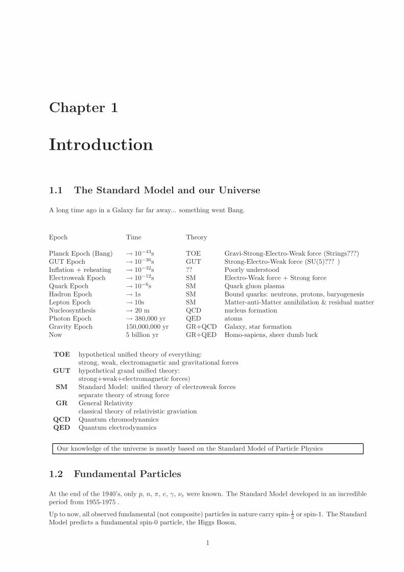
1.1 The Standard Model and our Universe

A long time ago in a Galaxy far far away... something went Bang.

Epoch Time Theory

Planck Epoch (Bang) → 10−43s TOE Gravi-Strong-Electro-Weak force (Strings???)GUT Epoch → 10−36s GUT Strong-Electro-Weak force (SU(5)??? )Inflation + reheating → 10−32s ?? Poorly understoodElectroweak Epoch → 10−12s SM Electro-Weak force + Strong forceQuark Epoch → 10−6s SM Quark gluon plasmaHadron Epoch → 1s SM Bound quarks: neutrons, protons, baryogenesisLepton Epoch → 10s SM Matter-anti-Matter annihilation & residual matterNucleosynthesis → 20 m QCD nucleus formationPhoton Epoch → 380,000 yr QED atomsGravity Epoch 150,000,000 yr GR+QCD Galaxy, star formationNow 5 billion yr GR+QED Homo-sapiens, sheer dumb luck

TOE hypothetical unified theory of everything:strong, weak, electromagnetic and gravitational forces

GUT hypothetical grand unified theory:strong+weak+electromagnetic forces)

SM Standard Model: unified theory of electroweak forcesseparate theory of strong force

GR General Relativityclassical theory of relativistic graviation

QCD Quantum chromodynamicsQED Quantum electrodynamics

Our knowledge of the universe is mostly based on the Standard Model of Particle Physics

1.2 Fundamental Particles

At the end of the 1940’s, only p, n, π, e, γ, νe were known. The Standard Model developed in an incredibleperiod from 1955-1975 .

Up to now, all observed fundamental (not composite) particles in nature carry spin- 12 or spin-1. The Standard

Model predicts a fundamental spin-0 particle, the Higgs Boson.

1

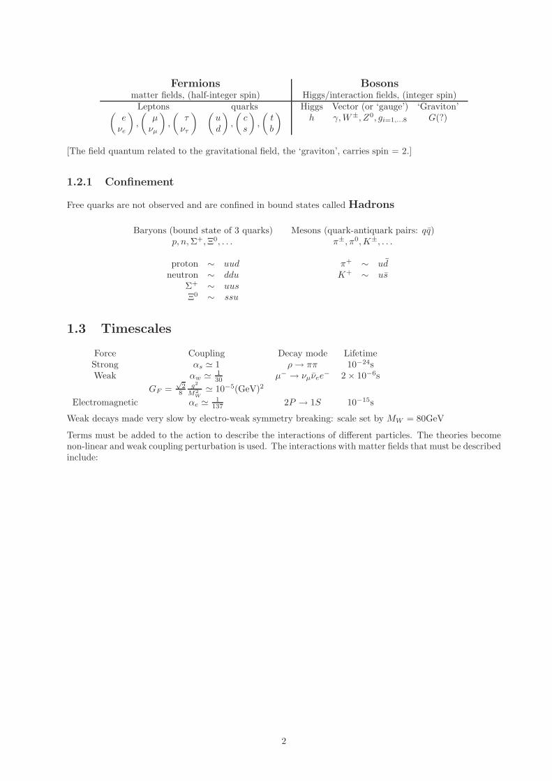
Fermions Bosonsmatter fields, (half-integer spin) Higgs/interaction fields, (integer spin)

Leptons quarks(eνe

),

(µνµ

),

(τντ

) (ud

),

(cs

),

(tb

) Higgs Vector (or ‘gauge’) ‘Graviton’h γ,W±, Z0, gi=1,...8 G(?)

[The field quantum related to the gravitational field, the ‘graviton’, carries spin = 2.]

1.2.1 Confinement

Free quarks are not observed and are confined in bound states called Hadrons

Baryons (bound state of 3 quarks) Mesons (quark-antiquark pairs: qq)p, n,Σ+,Ξ0, . . . π±, π0,K±, . . .

proton ∼ uudneutron ∼ ddu

Σ+ ∼ uusΞ0 ∼ ssu

π+ ∼ udK+ ∼ us

1.3 Timescales

Force Coupling Decay mode LifetimeStrong αs ≃ 1 ρ→ ππ 10−24sWeak αw ≃ 1

30 µ− → νµνee− 2× 10−6s

GF =√

28

g2

M2W

≃ 10−5(GeV)2

Electromagnetic αe ≃ 1137 2P → 1S 10−15s

Weak decays made very slow by electro-weak symmetry breaking: scale set by MW = 80GeV

Terms must be added to the action to describe the interactions of different particles. The theories becomenon-linear and weak coupling perturbation is used. The interactions with matter fields that must be describedinclude:

2

1.4 Interactions

Relative strength

a) Electromagnetic

e−

e−

γ

p

p

∼ 10−2

b) Weak

νe

e−

W

p

n

,

νµ

νµ

Z

e−

e−

∼ 10−5

c) Strong

u

u

q

d

d

no free quarks seen!

‘confinement’

∼ 1

d) Yukawa

t

t

h

b

b

e) Higgs

t

t

Z

Z

,

h

h

h

h

h

not seen yet

We also find we must describe self-interactions for gauge bosons when treating non-abelian gauge groupssuch as SU(N).

3

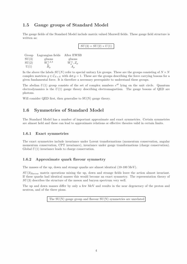
1.5 Gauge groups of Standard Model

The gauge fields of the Standard Model include matrix valued Maxwell fields. These gauge field structure iswritten as:

SU(3)× SU(2)× U(1)

Group Lagrangian fields After EWSBSU(3) gluons gluonsSU(2) W 1,2,3

µ W±µ , Zµ

U(1) Bµ Aµ

In the above the labels SU(N) refer to special unitary Lie groups. These are the groups consisting of N ×Ncomplex matrices g ∈ CN×N with det g = 1. These are the groups describing the force carrying bosons for agiven fundamental force. It is therefore a necessary prerequisite to understand these groups.

The abelian U(1) group consists of the set of complex numbers eiθ lying on the unit circle. Quantumelectrodynamics is the U(1) gauge theory describing electromagnetism. The gauge bosons of QED arephotons.

Will consider QED first, then generalise to SU(N) gauge theory.

1.6 Symmetries of Standard Model

The Standard Model has a number of important approximate and exact symmetries. Certain symmetriesare almost held and these can lead to approximate relations or effective theories valid in certain limits.

1.6.1 Exact symmetries

The exact symmetries include invariance under Lorent transformations (momentum conservation, angularmomentum conservation, CPT invariance), invariance under gauge transformations (charge conservation).Global U(1) invariance leads to charge conservation.

1.6.2 Approximate quark flavour symmetry

The masses of the up, down and strange quarks are almost identical (10-100 MeV).

SU(3)flavour matrix operations mixing the up, down and strange fields leave the action almost invariant.If these quarks had identical masses this would become an exact symmetry. The representation theory ofSU(3) describes the structure of the meson and baryon spectrum very well.

The up and down masses differ by only a few MeV and results in the near degeneracy of the proton andneutron, and of the three pions.

The SU(N) gauge group and flavour SU(N) symmetries are unrelated

4

Chapter 2

Free scalars, fermions, gauge bosons

c→∞N→∞ c→∞N→∞

~→0

~→0 QuantumMechanics

ClassicalMechanics

RelativisticQuantum

Field Theory

RelativisticField Theory

where N is the number of degrees of freedom, c is the speed of light, and ~ is Planck’s constant.

A field theory is a continuum generalisation of (discrete) point-particle mechanics

qi(t) with i ∈ 1, . . . , N generalised coordinate → φ(x, t)pi(t) = ∂L

∂qicanonical momentum → π(x, t) = δL

δφ

L(qi, qi) Lagrange function → L =∫d3x L(φ(x), ∂µφ(x))

Action: S =

∫d4x L(φ, ∂µφ) where L ≡ “Lagrangian Density”

2.1 Free fields

Minimising action means δS = 0 under arbitrary change δφ vanishing at infinity ⇒ equations of motion:

δS =

∫d4x

[(∂L

∂(∂µφ)

)∂µδφ+

∂L∂φ

δφ

]= 0 ⇔ ∂µ

(∂L

∂(∂µφ)

)− ∂L∂φ

= 0

where we give our conventions as

∂µ ≡∂

∂xµ=( ∂∂t,∇), aµ = gµνaν , and gµν ≡

1 0 0 00 −1 0 00 0 −1 00 0 0 −1

2.1.1 Noethers theorem

Symmetries of action ⇒ conserved currents

5

A change in the field(s) induces a change in the Lagrangian.

ϕ→ ϕ′ = ϕ+ δϕ

ϕ∗ → ϕ′∗ = ~ϕ∗ + δ~ϕ∗

If the change in the field is chosen to be a symmetry of the Lagrangian invariance means

0 = δL = L(~ϕ ′, ~ϕ ′†, ∂µ~ϕ

′, ∂µ~ϕ′†)− L

(~ϕ, ~ϕ†, ∂µ~ϕ, ∂µ~ϕ

†)

This leads to

δL =∂L∂ϕj

δϕj +∂L

∂(∂µϕj

)δ(∂µϕj

)+

∂L∂ϕ∗

j

δϕ∗j +

∂L∂(∂µϕ∗

j

)δ(∂µϕ

∗j

)

=∂L∂ϕj

δϕj + ∂µ

( ∂L∂(∂µϕj

)δϕj

)− ∂µ

( ∂L∂(∂µϕj

))δϕj+

+∂L∂ϕ∗

j

δϕ∗j + ∂µ

( ∂L∂(∂µϕ∗

j

)δϕ∗j

)− ∂µ

( ∂L∂(∂µϕ∗

j

))δϕ∗

j

= ∂µ

( ∂L∂(∂µϕj

)δϕj

)+ ∂µ

( ∂L∂(∂µϕ∗

j

)δϕ∗j

)← terms vanish due to the eqns of motion

= ∂µJµ

Jµ is a conserved current because ∫d3x∂µJµ =

∂

∂t

∫d3xJ0 = 0

2.1.2 Free field actions

1. Real scalar field (spin-0 particles: π0, Higgs boson, . . . )

L =1

2∂µφ∂

µφ− 1

2m2φ2 ⇒ (∂2 +m2)φ = 0

2. Complex scalar field (π±, K±, . . . , spin-0 charged particles)

L =1

2∂µφ

∗∂µφ− 1

2m2φ∗φ ⇒ (∂2 +m2)φ(∗) = 0

3. Maxwell field (spin-1 particles: γ, . . . )

L = −1

4FµνFµν ⇒ ∂µFµν = 0

with

Fµν ≡ ∂µAν − ∂νAµ =

0 −E1 −E2 −E3

E1 0 −B3 B1

E2 B3 0 −B2

E3 −B1 B2 0

and

E = −∇ ·A− ∂

∂tA and B = ∇×A

Note that using the equation of motion and the Bianchi identity, ∂ρFµν + ∂µF νρ + ∂νF ρµ = 0, we canobtain Maxwell’s equations: ∇ ·

(E,B

)= 0,∇×

(E,B

)= ∂

∂t

(−B,E

).

6

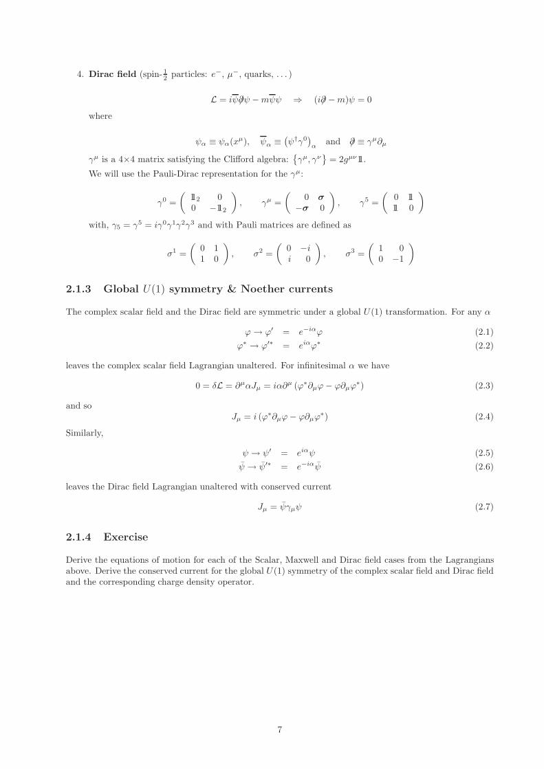
4. Dirac field (spin- 12 particles: e−, µ−, quarks, . . . )

L = iψ∂/ψ −mψψ ⇒ (i∂/−m)ψ = 0

where

ψα ≡ ψα(xµ), ψα ≡(ψ†γ0

)α

and ∂/ ≡ γµ∂µ

γµ is a 4×4 matrix satisfying the Clifford algebra:γµ, γν

= 2gµν11.

We will use the Pauli-Dirac representation for the γµ:

γ0 =

(112 00 −112

), γµ =

(0 σ

−σ 0

), γ5 =

(0 1111 0

)

with, γ5 = γ5 = iγ0γ1γ2γ3 and with Pauli matrices are defined as

σ1 =

(0 11 0

), σ2 =

(0 −ii 0

), σ3 =

(1 00 −1

)

2.1.3 Global U(1) symmetry & Noether currents

The complex scalar field and the Dirac field are symmetric under a global U(1) transformation. For any α

ϕ→ ϕ′ = e−iαϕ (2.1)

ϕ∗ → ϕ′∗ = eiαϕ∗ (2.2)

leaves the complex scalar field Lagrangian unaltered. For infinitesimal α we have

0 = δL = ∂µαJµ = iα∂µ (ϕ∗∂µϕ− ϕ∂µϕ∗) (2.3)

and soJµ = i (ϕ∗∂µϕ− ϕ∂µϕ

∗) (2.4)

Similarly,

ψ → ψ′ = eiαψ (2.5)

ψ → ψ′∗ = e−iαψ (2.6)

leaves the Dirac field Lagrangian unaltered with conserved current

Jµ = ψγµψ (2.7)

2.1.4 Exercise

Derive the equations of motion for each of the Scalar, Maxwell and Dirac field cases from the Lagrangiansabove. Derive the conserved current for the global U(1) symmetry of the complex scalar field and Dirac fieldand the corresponding charge density operator.

7

Chapter 3

Abelian gauge theory

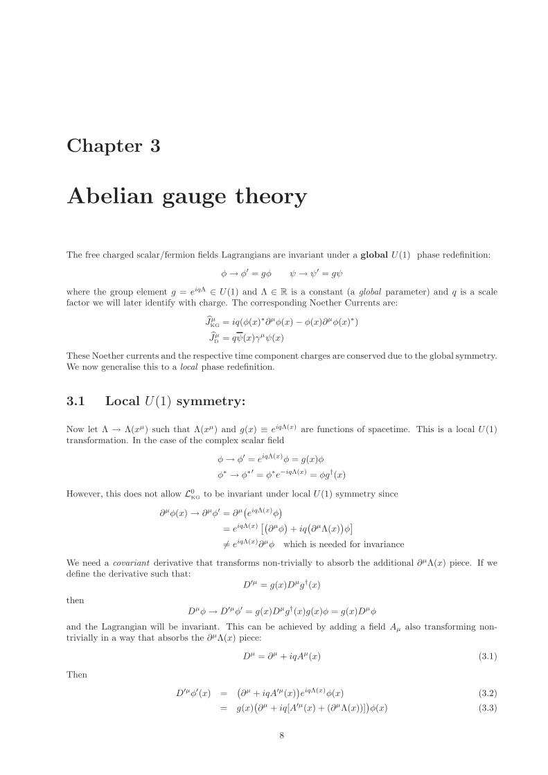
The free charged scalar/fermion fields Lagrangians are invariant under a global U(1) phase redefinition:

φ→ φ′ = gφ ψ → ψ′ = gψ

where the group element g = eiqΛ ∈ U(1) and Λ ∈ R is a constant (a global parameter) and q is a scalefactor we will later identify with charge. The corresponding Noether Currents are:

JµKG = iq(φ(x)∗∂µφ(x) − φ(x)∂µφ(x)∗)

JµD

= qψ(x)γµψ(x)

These Noether currents and the respective time component charges are conserved due to the global symmetry.We now generalise this to a local phase redefinition.

3.1 Local U(1) symmetry:

Now let Λ → Λ(xµ) such that Λ(xµ) and g(x) ≡ eiqΛ(x) are functions of spacetime. This is a local U(1)transformation. In the case of the complex scalar field

φ→ φ′ = eiqΛ(x)φ = g(x)φ

φ∗ → φ∗′ = φ∗e−iqΛ(x) = φg†(x)

However, this does not allow L0KG to be invariant under local U(1) symmetry since

∂µφ(x)→ ∂µφ′ = ∂µ(eiqΛ(x)φ

)

= eiqΛ(x)[(∂µφ

)+ iq

(∂µΛ(x)

)φ]

6= eiqΛ(x)∂µφ which is needed for invariance

We need a covariant derivative that transforms non-trivially to absorb the additional ∂µΛ(x) piece. If wedefine the derivative such that:

D′µ = g(x)Dµg†(x)

thenDµφ→ D′µφ′ = g(x)Dµg†(x)g(x)φ = g(x)Dµφ

and the Lagrangian will be invariant. This can be achieved by adding a field Aµ also transforming non-trivially in a way that absorbs the ∂µΛ(x) piece:

Dµ = ∂µ + iqAµ(x) (3.1)

Then

D′µφ′(x) =(∂µ + iqA′µ(x)

)eiqΛ(x)φ(x) (3.2)

= g(x)(∂µ + iq[A′µ(x) + (∂µΛ(x))]

)φ(x) (3.3)

8

Thus, if we define the transformation law for Aµ as

A′µ(x) = Aµ(x) − ∂µΛ(x) (3.4)

we obtain D′µφ′ = g(x)Dµφ as required.

This is just a gauge transformation of the vector potential Aµ!

If we couple a globally U(1) symmetric theory to a gauge field Aµ by this covariant derivative one ends upwith a locally symmetric U(1) theory. This way of coupling a gauge potential to a matter field is traditionallycalled principle of minimal coupling. In the context of gauge theories it is deduced from the local invarianceproperty.

The free Klein-Gordon Lagrangian becomes

L0KG→ L

KG= (Dµφ)∗(Dµφ) −m2φ∗φ

= [(∂µ − iqAµ)φ∗](∂µ + iqAµ)φ−m2φ∗φ

= ∂µφ∗∂µφ+ iq(∂µφ

∗)φAµ − iqAµφ∗∂µφ+ q2AµA

µφ∗φ−m2φ∗φ

= L0KG + LInteraction

where we define LInteraction as

LInteraction ≡ JµKGAµ + q2AµA

µφ∗φ

Now we see that our theory which is invariant under local gauge transformations is promoted to an interactingtheory. Hence we conclude locally symmetric theories induce uniquely defined interaction properties.

Local gauge symmetry ⇒ matter-gauge field interaction

3.1.1 Gauge action

The dynamics of the gauge field Aµ is induced in the standard way:

Fµν = ∂µAν − ∂νAµ = −(i/q)[Dµ, Dν ] (tutorial)

LMaxwell = −1

4FµνFµν

where Fµν is constructed to be gauge invariant as it is symmetric under a U(1) gauge transformation:Aµ → Aµ′ = Aµ − ∂µΛ.

3.2 Scalar electrodynamics

The full Lagrangian to describe a free complex scalar field is thus given by

L = LMaxwell

+ LKG

= LMaxwell

+ L0KG

+ LInteraction

This is known as Scalar Electrodynamics. It is the first example of a non-trivial field theory based on acommuting symmetry group and is hence an example of an Abelian Gauge Theory.

The field equations are obtained by the principle of least action δS = 0 from the action S =∫d4xL . The

gauge covariant field equation for the complex scalar field is

(DµDµ +m2)φ = 0

For the gauge field Aµ we find from ∂µ

(δL

δ∂µAν

)= δL

δAν

∂µFµν = ∂2Aν − ∂ν(∂µA

µ) = Jν ,

9

with

Jν = −∂LInt

∂Aν

= iq(φ∗Dνφ− φDνφ∗)

= JKG − 2q2φ∗φAµ

We see that Jµ is the covariant generalisation of the Noether Current:

JKG

∂µ→Dµ

−−−−−→ Jν

Along with the Bianchi Identity∂µF νρ + ∂νF ρµ + ∂ρFµν = 0

the gauge field equation of motion leads to Maxwell’s equations.

3.3 Quantum electrodynamics

We now consider the case of a fermion fields

ψ(x)→ ψ(x)′ = g(x)ψ(x)

ψ(x)→ ψ(x)′= ψ(x)g†(x)

along with the covariant derivative given in the last lecture

Dµ = ∂µ + iqAµ

The covariant Dirac field Lagrangian is

L0D→ L

D= iψγµD

µψ −mψψ= iψγµ∂

µψ −mψψ + LInt

= L0D

+ LInt

LInt = −JµAµ with Jµ = Qψγµψ

As before the kinetic term for the gauge field is given by the Maxwell Lagrangian. The full locally invariantLagrangian is now

L = LMax

+ LD

= LMax

+ L0D

+ LInt

The field equation for the Dirac field is

(iD/−m)ψ(x) = 0

and as before the gauge field equation is,

∂µFµν = ∂2Aν − ∂ν(∂µA

µ) = Jν .

Remarks

1. To solve ∂2Aν − ∂ν(∂µAµ) = Jν we cannot invert the operator and thus we must introduce a

gauge-fixing term:L

G.F.= −λ(∂µA

µ)2 (see tutorial)

2. We are unable to add a photon mass term since it is not gauge invariant

Lmass

=1

2m2

γAµAµ Aµ′=Aµ−∂µΛ−−−−−−−−−→ 1

2m2

γ(AµAµ − 2Aµ∂

µΛ + ∂µΛ∂µAµ) 6= 1

2m2

γAµAµ

Mass terms of gauge bosons destroy gauge invariance !!!

10

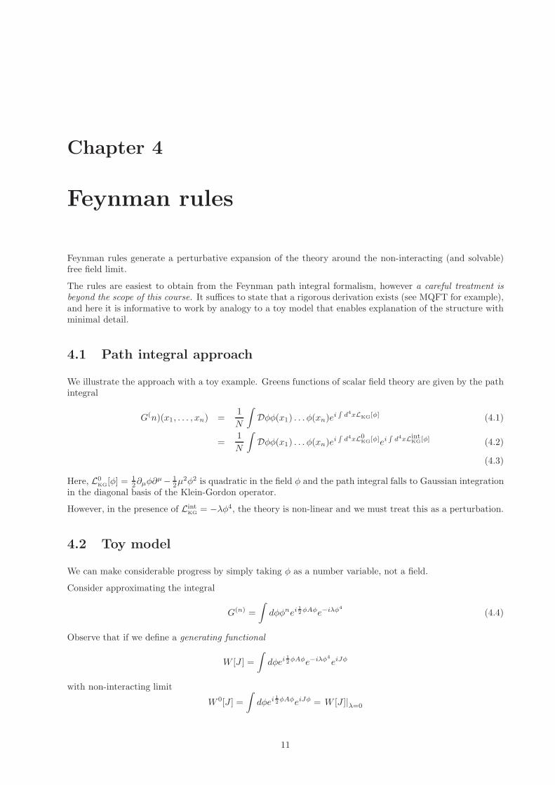
Chapter 4

Feynman rules

Feynman rules generate a perturbative expansion of the theory around the non-interacting (and solvable)free field limit.

The rules are easiest to obtain from the Feynman path integral formalism, however a careful treatment isbeyond the scope of this course. It suffices to state that a rigorous derivation exists (see MQFT for example),and here it is informative to work by analogy to a toy model that enables explanation of the structure withminimal detail.

4.1 Path integral approach

We illustrate the approach with a toy example. Greens functions of scalar field theory are given by the pathintegral

G(n)(x1, . . . , xn) =1

N

∫Dφφ(x1) . . . φ(xn)ei

R

d4xLKG[φ] (4.1)

=1

N

∫Dφφ(x1) . . . φ(xn)ei

R

d4xL0KG[φ]ei

R

d4xLintKG[φ] (4.2)

(4.3)

Here, L0KG

[φ] = 12∂µφ∂

µ− 12µ

2φ2 is quadratic in the field φ and the path integral falls to Gaussian integrationin the diagonal basis of the Klein-Gordon operator.

However, in the presence of LintKG

= −λφ4, the theory is non-linear and we must treat this as a perturbation.

4.2 Toy model

We can make considerable progress by simply taking φ as a number variable, not a field.

Consider approximating the integral

G(n) =

∫dφφnei 1

2 φAφe−iλφ4

(4.4)

Observe that if we define a generating functional

W [J ] =

∫dφei 1

2φAφe−iλφ4

eiJφ

with non-interacting limit

W 0[J ] =

∫dφei 1

2φAφeiJφ = W [J ]|λ=0

11

then we can generate all correlation functions by differentiating with respect to the source J

G(n) =dn

d(iJ)nW [J ]

∣∣∣∣J=0

=dn

d(iJ)ne−iλ d4

d(iJ)4 W 0[J ]

∣∣∣∣J=0

(4.5)

After completing the square i 12φAφ+iJφ = i 12A(φ+A−1J)2−i 12JA−1J the integralW 0[J ] can be performedby Gaussian integration (if we add an iǫφ2 term to give a negative real part to exponent) and gives

W 0[J ] = N ′e−i 12 J(A+iǫ)−1J

where N ′ is a new, and also irrelevant normalisation.

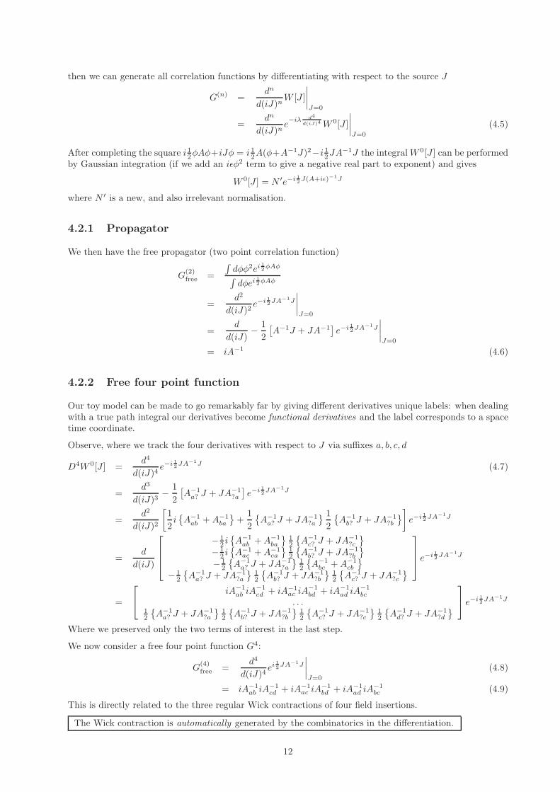
4.2.1 Propagator

We then have the free propagator (two point correlation function)

G(2)free =

∫dφφ2ei 1

2φAφ

∫dφei 1

2φAφ

=d2

d(iJ)2e−i 1

2JA−1J

∣∣∣∣J=0

=d

d(iJ)− 1

2

[A−1J + JA−1

]e−i 1

2JA−1J

∣∣∣∣J=0

= iA−1 (4.6)

4.2.2 Free four point function

Our toy model can be made to go remarkably far by giving different derivatives unique labels: when dealingwith a true path integral our derivatives become functional derivatives and the label corresponds to a spacetime coordinate.

Observe, where we track the four derivatives with respect to J via suffixes a, b, c, d

D4W 0[J ] =d4

d(iJ)4e−i 1

2JA−1J (4.7)

=d3

d(iJ)3− 1

2

[A−1

a? J + JA−1?a

]e−i 1

2JA−1J

=d2

d(iJ)2

[1

2iA−1

ab +A−1ba

+

1

2

A−1

a? J + JA−1?a

1

2

A−1

b? J + JA−1?b

]e−i 1

2 JA−1J

=d

d(iJ)

− 12 iA−1

ab +A−1ba

12

A−1

c? J + JA−1?c

− 12 iA−1

ac +A−1ca

12

A−1

b? J + JA−1?b

− 12

A−1

a? J + JA−1?a

12

A−1

bc +A−1cb

− 12

A−1

a? J + JA−1?a

12

A−1

b? J + JA−1?b

12

A−1

c? J + JA−1?c

e

−i 12 JA−1J

=

iA−1ab iA

−1cd + iA−1

ac iA−1bd + iA−1

ad iA−1bc

. . .12

A−1

a? J + JA−1?a

12

A−1

b? J + JA−1?b

12

A−1

c? J + JA−1?c

12

A−1

d? J + JA−1?d

e−i 1

2 JA−1J

Where we preserved only the two terms of interest in the last step.

We now consider a free four point function G4:

G(4)free =

d4

d(iJ)4ei 1

2JA−1J

∣∣∣∣J=0

(4.8)

= iA−1ab iA

−1cd + iA−1

ac iA−1bd + iA−1

ad iA−1bc (4.9)

This is directly related to the three regular Wick contractions of four field insertions.

The Wick contraction is automatically generated by the combinatorics in the differentiation.

12

4.2.3 Perturbative expansion

We can now expand in the coupling λ

e−iλ d4

d(iJ)4 W 0[J ] = (1− iλ d4

d(iJ)4)W 0[J ] ≡ ∗1 + iLint

KG)W 0[J ]

As interaction terms are local a field theory, we consider all derivatives as equivalent in the last term

−iλ d4

d(iJ)4)W 0[J ] ∼ −iλ

(1

2

A−1

e? J + JA−1?e

1

2

A−1

e? J + JA−1?e

1

2

A−1

e? J + JA−1?e

1

2

A−1

e? J + JA−1?e

)e−i 1

2 JA−1J

If we now form the O(λ1) piece of G4 (formally the connected O(λ1) piece as we dropped some terms)

δG4 =d4

d(iJ)4− iλ

(1

2

A−1

e? J + JA−1?e

1

2

A−1

e? J + JA−1?e

1

2

A−1

e? J + JA−1?e

1

2

A−1

e? J + JA−1?e

)e−i 1

2 JA−1J

∣∣∣∣J=0

= −iλ

iA−1ea iA

−1eb iA

−1ec iA

−1ed + iA−1

ea iA−1eb iA

−1ed iA

−1ec

iA−1ea iA

−1ec iA

−1eb iA

−1ed + iA−1

ea iA−1ed iA

−1eb iA

−1ec

iA−1ea iA

−1ec iA

−1ed iA

−1eb + iA−1

ea iA−1ed iA

−1ec iA

−1eb

. . .iA−1

eb iA−1ec iA

−1ed iA

−1ea + iA−1

eb iA−1ed iA

−1ec iA

−1ea

iA−1ec iA

−1eb iA

−1ed iA

−1ea + iA−1

ed iA−1eb iA

−1ec iA

−1ea

iA−1ec iA

−1ed iA

−1eb iA

−1ea + iA−1

ed iA−1ec iA

−1eb iA

−1ea

(4.10)

In this case the symmetrisation created by different ways to take derivatives creates an overall factor of 4!in the vertex rule −iλ4!.

The above toy model bears a direct mapping to the formal derivation in a path integral context where φ,A, Jall becomes functions of a space-time coordinate. When A becomes a differential operator, it is diagonal inthe momentum basis and the separate Gaussian integrals for each mode may be performed just as above.Our lessons can be summarised

Propagator rules: take i times inverse of operators in quadratic terms in L0

Interaction vertex rules: differentiate iLint w.r.t. each field. Differentiation automatically symmetrises

4.3 Feynman Rules and Feynman Diagrams

Quantum field theory leads to computational “Feynman” rules to evaluate the S−matrix elements: Sif =

〈i|S|f〉 where S is the scattering operator (see further lectures). Each term in a Lagrangian that containsproducts of fields, ϕ1, . . . , ϕN ;ϕj ∈

φ, ψ,Aµ

, leads to an n-point vertex :

We outline a procedure for determining the Feynman rules in a four dimensional relativistic Field theory.

1. Break the Lagrangian into a sum of distinct terms L =∑

j Lj

These will be composed ofa) quadratic terms which define the free theory around which we expandb) higher order terms defining the non-linear interaction Lagrangian

2. For each term express∫d4xL| in terms of incoming momenta e.g. φ(x) = e−iqµxµ

φ(qa)Translational invariance of Lagrangian gives an overall momentum conserving delta functionReplaces ∂µ → −ikµ and multiplies by (2π4)δ4(

∑q).

3. Take functional derivatives with respect to corresponding set of fields φ(kb)

13

φ4(x4)

φn(xn)φ2(x2)

φ1(x1)

φ3(x3)

∼ Vφ1...φn(x1, . . . , xn) =

δ

δφ1(x1)· · · δ

δφn(xn)

(i

∫d4xL

)

→ produces same combinatorial factors/symmetrisation as above toy model suggests→ For propagator take i× (2-vertex)−1 setting→ For interaction vertex take i× n-vertex

It may take working out an example to see that the combinatorics of (i) an un-motivated functional differ-entiation and (ii) the combinatorics of the (toy model for) path integral above, work out the same.

To illustrate this we will apply the method to the scalar propagator for L0KG

= 12∂µφ∂

µφ− 12µ

2φ2

4.3.1 Full speed

Step 2:

−1

2φ(q1)(q1µq

µ2 + µ2)φ(q2)(2π)4δ4(q1 + q2)

Step 3:i(kµk

µ − µ2)−1

Now the Feynman propagator is

G(k) =i

kµkµ − µ2

k

⇔ G(k) =i

k2 −m2 + iǫ

4.3.2 Slow motion replay

Step 2:∫d4xL0

KG =

∫d4x

[1

2∂µφ(x)∂µφ(x) − 1

2µ2φ2(x)

]

=

∫d4q1

∫d4q2

∫d4x

[1

2∂µφ(q1)e

−iqα2 xα∂µe−iqν

2 xνφ(q2)−1

2µ2φ(q1)φ(q2)e

−iqα2 xαe−iqν

2 xν

]

=

∫d4q1

∫d4q2

[−1

2qµ1 q2µφ(q1)φ(q2)−

1

2µ2φ(q1)φ(q2)

]×∫d4xe−iqα

2 xαe−iqν2 xν

=

∫d4q1

∫d4q2

[−1

2qµ1 q2µ −

1

2µ2

]φ(q1)φ(q2)(2π)4δ4(q1 + q2) (4.11)

Step 3:

δ

δφ(k1)

δ

δφ(k2)

Z

d4xL0KG =

Z

d4q1

Z

d4q2

»

−1

2qµ1 q2µ −

1

2µ2

– »

δ4(q1 − k1)δ4(q2 − k2)

+ δ4(q1 − k2)δ4(q2 − k1)

–

(2π)4δ4(q1 + q2)

=ˆ

−kµ1 k2µ − µ2

˜

(2π)4δ4(k1 + k2)

≡ˆ

kµkµ − µ2˜

Where for the last step we either integrate over k2 or simply know that we will take k1 = −k2 = k to conservemomentum in the propagator.

14

4.3.3 Feynman rules for QED

Note that momentum is conserved at each vertex.

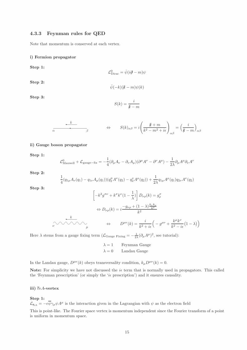
i) Fermion propagator

Step 1:L0

Dirac = ψ(i∂/−m)ψ

Step 2:ψ(−k)(/k −m)ψ(k)

Step 3:

S(k) =i

/k −m

α β

k

⇔ S(k)αβ = i

(k/+m

k2 −m2 + iǫ

)

αβ

=( i

k/ −m)

αβ

ii) Gauge boson propagator

Step 1:

L0Maxwell + Lgauge−fix = −1

4(∂µAν − ∂νAµ)(∂µAν − ∂νAµ)− 1

2λ∂µA

µ∂νAν

Step 2:1

4(q1µAν(q1)− q1νAµ(q1))(q

µ2A

ν(q2)− qν2A

µ(q2)) +1

2λq1µA

µ(q1)q2νAν(q2)

Step 3: [−k2gσν + kσkν(1− 1

λ)

]Dνρ(k) = gσ

ρ

⇔ Dνρ(k) = i−gνρ + (1− λ)kν kρ

k2

k2

k

µν⇔ Dµν(k) =

i

k2 + iǫ

(− gµν +

kµkν

k2 − iǫ(1− λ

))

Here λ stems from a gauge fixing term (LGauge Fixing = − 12λ(∂µA

µ)2, see tutorial):

λ = 1 Feynman Gauge

λ = 0 Landau Gauge

In the Landau gauge, Dµν(k) obeys transversality condition, kµDµν(k) = 0.

Note: For simplicity we have not discussed the iǫ term that is normally used in propagators. This calledthe ‘Feynman prescription’ (or simply the ‘iǫ prescription’) and it ensures causality.

iii) eeA-vertex

Step 1:LeeA = −eψγµψA

µ is the interaction given in the Lagrangian with ψ as the electron field

This is point-like. The Fourier space vertex is momentum independent since the Fourier transform of a pointis uniform in momentum space.

15

Step 2:

−eψ(k1)γµψ(k2)Aµ(k3)

Step 3:

−ie(γµ)αβ

β

α

∼ −ie(γµ)αβ

Diagrammatically we have

4.3.4 External particles and external lines

We adopt the convention of having the charge and momentum parallel in the electron and anti-parallel inthe positron.

Incoming Outgoing

electron:α

k

∼ [us(k)]αα

k

∼ [us(k)]α

positron:α

k

∼ [vs(k)]αα

k

∼ [vs(k)]α

photon:µ

k

∼ ελµ(k)

µ

k

∼ ελ∗µ (k)

Spin and polarisation sums

If we are interested in the unpolarised cross-section only, we must average over the initial states and sumover all polarisations and spins for the unspecified final states.

initial states final states

spins1

2

∑

s

usus =1

2k/

∑

s′

u′s′u′s′ = k/′

polarisations1

2

∑

σ

εµσε

νσ∗ = −1

2gµν + · · ·

∑

σ′

ε′νσ′ε′

µσ′ = −gµν + · · ·

These summations convert a Feynman amplitude involving fermions into traces of “slashed” vectors

4.3.5 Dirac matrix manipulation

When conjugating terms involving spinors to square the amplitude we need the following:

γ†0 = γ0

γ†5 = γ5

γ0γ†µγ0 = γµ

16

Spin averaging Fermion line terms leads to Dirac traces. We give some rules for calculating such traces (seetutorial for more).

In doing so we apply the Clifford algebra property

γµ, γν

= 2gµν

Using this we find for example

tr(p/1γ

µp/2 · · ·)

= tr(p/1

γµ, p/2

· · ·)− tr

(p/1p/2γ

µ · · ·)

= 2 pµ2 tr(p/1 · · ·

)− tr

(p/1p/2γ

µ · · ·)

Other useful properties:

γν/aγν = −2/a

γν/a/bγν = 4(a · b)1

γν/a/b/cγν = −2/c/b/a

tr(a/b/c/d/

)= 4

(a · b c · d− a · c b · d+ a · d b · c

)

tr(a/b/)

= 4(a · b

)

tr(a/1 · · · a/2k−1

)= 0

The following are useful when we come to deal with W and Z boson couplings:

tr(γµγνγργσ

)= 4(gµνgρσ − gµρgνσ + gµρgνσ)

tr(γ5γ

µγνγργσ)

= −4iǫµνρσ

ǫµνρσǫµναβ = −2(δραδ

σβ − δ

ρβδ

σα

)

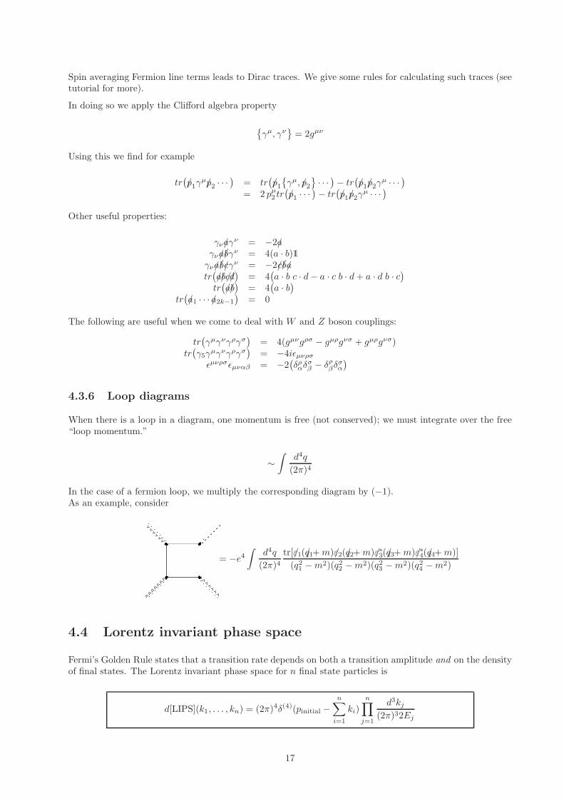
4.3.6 Loop diagrams

When there is a loop in a diagram, one momentum is free (not conserved); we must integrate over the free“loop momentum.”

∼∫

d4q

(2π)4

In the case of a fermion loop, we multiply the corresponding diagram by (−1).As an example, consider

= −e4∫

d4q

(2π)4tr[ε1/ (q1/+m)ε2/ (q2/+m)ε∗3/ (q3/ +m)ε∗4/ (q4/ +m)]

(q21 −m2)(q22 −m2)(q23 −m2)(q24 −m2)

4.4 Lorentz invariant phase space

Fermi’s Golden Rule states that a transition rate depends on both a transition amplitude and on the densityof final states. The Lorentz invariant phase space for n final state particles is

d[LIPS](k1, . . . , kn) = (2π)4δ(4)(pinitial −n∑

i=1

ki)

n∏

j=1

d3kj

(2π)32Ej

17

Where E2j = |kj |2 +m2

j satisfies the on-shell energy momentum relation. The above is all that is requiredfor calculation, however, the Lorentz invariance is manifest when re-written as

d[LIPS](k1, . . . , kn) = (2π)4δ(4)(p1 + p2 −n∑

i=1

ki)

n∏

j=1

δ+(k2j −m2

j)d4kj

(2π)3

where

δ+(kj −m2j) ≡Θ(k0

j)δ(k2j −m2

j)

=Θ(k0

j)δ((k0

j − ωj)(k0

j + ωj))

=Θ(k0

j)

2ωjδ(k0

j − ωj) where ωj =√

k2j −m2

j

4.4.1 Cross-section phase space

We need Lorentz invariant cross-sections for 2 particles scattering two n final state particles.

p1

p2

k1

kn

〈k1, . . . , kn|S|p1p2〉 = 〈f |S|i〉

〈f |S|i〉 = δfi︸︷︷︸needed for f=i

−(2π)4δ(4)(p1 + p2 −n∑

j=1

kj)∣∣Mi→f

∣∣2

The general differential cross-section is

dσ =ζ

2√λ(s,m2

1,m22)

∣∣Mi→f

∣∣2d[LIPS](k1, . . . , kn)

Here p21 = m2

1, p22 = m2

2, s = (p1 + p2)2, and ζ is the symmetry factor, which avoid overcounting in case of

identical particles in the final state. For n identical particles in the final state it is ζ = 1/n!. For two sets(n1, n2) of identical particles it is ζ = 1/(n1!n2!).

The Kaellen Function is defined by:

λ(s,m21,m

22) =s2 +m4

1 +m42 − 2s(m2

1 +m22)− 2m2

1m22

=s(s− 2(m2

1 +m22))

+ (m21 −m2

2)2

When s≫ m1,m2 we have

dσ =ζ

2s

∣∣Mi→f

∣∣2d[LIPS](k1, . . . , kn)

For exam purposes only this limit need be remembered

4.4.2 Decay phase space

Decay of a particle with mass M : p2 = M2

18

p

k1

kn

〈k1, . . . , kn|S|p〉 = δfi − (2π)4δ(4)(p1 + p2 −n∑

j=1

kj)∣∣Mi→f

∣∣2

dΓ in the rest frame of the decaying particle where p = (M, 0)

dΓ =ζ

2M

∣∣Mi→f

∣∣2d[LIPS](k1, . . . , kn)

19

Chapter 5

Leading order processes

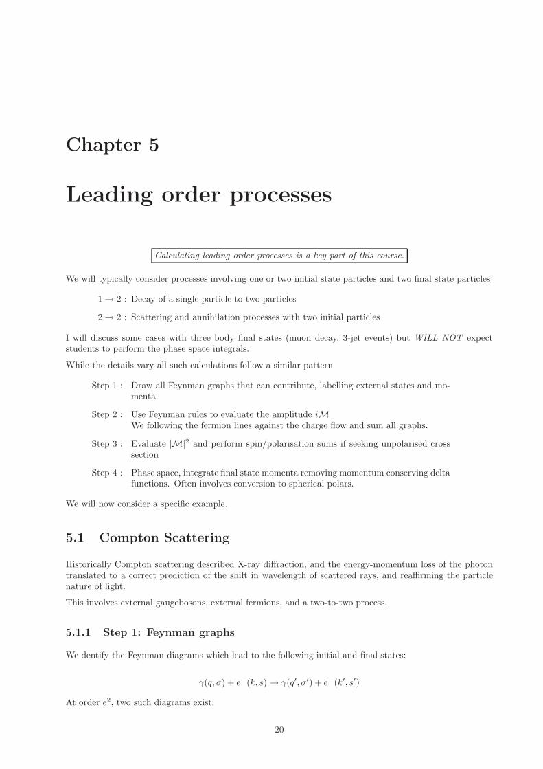
Calculating leading order processes is a key part of this course.

We will typically consider processes involving one or two initial state particles and two final state particles

1→ 2 : Decay of a single particle to two particles

2→ 2 : Scattering and annihilation processes with two initial particles

I will discuss some cases with three body final states (muon decay, 3-jet events) but WILL NOT expectstudents to perform the phase space integrals.

While the details vary all such calculations follow a similar pattern

Step 1 : Draw all Feynman graphs that can contribute, labelling external states and mo-menta

Step 2 : Use Feynman rules to evaluate the amplitude iMWe following the fermion lines against the charge flow and sum all graphs.

Step 3 : Evaluate |M|2 and perform spin/polarisation sums if seeking unpolarised crosssection

Step 4 : Phase space, integrate final state momenta removing momentum conserving deltafunctions. Often involves conversion to spherical polars.

We will now consider a specific example.

5.1 Compton Scattering

Historically Compton scattering described X-ray diffraction, and the energy-momentum loss of the photontranslated to a correct prediction of the shift in wavelength of scattered rays, and reaffirming the particlenature of light.

This involves external gaugebosons, external fermions, and a two-to-two process.

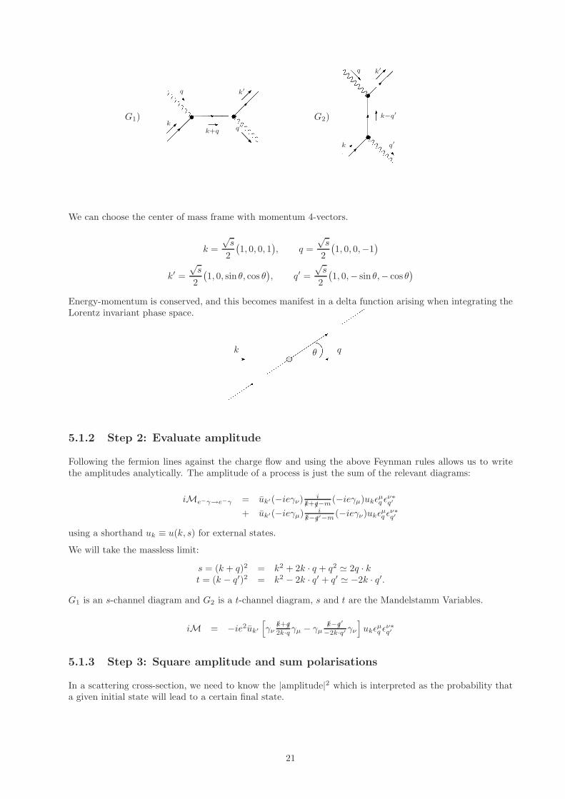
5.1.1 Step 1: Feynman graphs

We dentify the Feynman diagrams which lead to the following initial and final states:

γ(q, σ) + e−(k, s)→ γ(q′, σ′) + e−(k′, s′)

At order e2, two such diagrams exist:

20

G1)k

k′

k+q

q

q′G2)

k

k′

k−q′

q

q′

We can choose the center of mass frame with momentum 4-vectors.

k =

√s

2

(1, 0, 0, 1

), q =

√s

2

(1, 0, 0,−1

)

k′ =

√s

2

(1, 0, sin θ, cos θ

), q′ =

√s

2

(1, 0,− sin θ,− cos θ

)

Energy-momentum is conserved, and this becomes manifest in a delta function arising when integrating theLorentz invariant phase space.

k θ q

5.1.2 Step 2: Evaluate amplitude

Following the fermion lines against the charge flow and using the above Feynman rules allows us to writethe amplitudes analytically. The amplitude of a process is just the sum of the relevant diagrams:

iMe−γ→e−γ = uk′(−ieγν) i/k+/q−m

(−ieγµ)ukǫµq ǫ

ν∗q′

+ uk′(−ieγµ) i/k−/q′−m

(−ieγν)ukǫµq ǫ

ν∗q′

using a shorthand uk ≡ u(k, s) for external states.

We will take the massless limit:

s = (k + q)2 = k2 + 2k · q + q2 ≃ 2q · kt = (k − q′)2 = k2 − 2k · q′ + q′ ≃ −2k · q′.

G1 is an s-channel diagram and G2 is a t-channel diagram, s and t are the Mandelstamm Variables.

iM = −ie2uk′

[γν

/k+/q

2k·qγµ − γµ/k−/q

′

−2k·q′ γν

]ukǫ

µq ǫ

ν∗q′

5.1.3 Step 3: Square amplitude and sum polarisations

In a scattering cross-section, we need to know the |amplitude|2 which is interpreted as the probability thata given initial state will lead to a certain final state.

21

We can write the conjugate amplitude as

−iM† = −ie2u†k[γ†µ

(/k+/q)†

2k·q γ†ν − γ†ν(/k−/q

′)†

−2k·q′ γ†µ

]γ†0uk′ǫµ∗q ǫνq′

= −ie2u†kγ0

[γ0γ

†µγ0γ0

(/k+/q)†

2k·q γ0γ0γ†νγ0 − γ0γ

†νγ0γ0

(/k−/q′)†

−2k·q′ γ0γ0γ†µγ0

]uk′ǫµ∗q ǫνq′

= −ie2uk

[γµ

/k+/q

2k·qγν − γν/k−/q

′

−2k·q′ γµ

]uk′ǫµ∗q ǫνq′

and so

|M|2 = e4uk′

[γν

/k+/q


′

−2k·q′ γν

]ukuk

[γµ′

/k+/q

2k·qγν′ − γν′/k−/q

′

−2k·q′ γµ′

]uk′ǫµ

′∗q ǫν

′q′ ǫµq ǫ

ν∗q′

• The spin/polarisation dependence in∣∣M∣∣2 is obtained by using the expressions for us, us, ε

σ, ε′σ

• unpolarised probability found by averaging initial and summing final spins and polarisations

• The spin/polarisation sums produce factors of /k and −gµν

• We must carefully track indices so that the left side of /k contracts with the same matrixthat uk did, while the right side of /k contracts with the same index uk did.

• This leads to a trace.

• Each fermion line leads to a separate trace, and graphs with several fermion lines willgive the product of several traces.

12

∑s,s′

12

∑σ,σ′|M|2 = 1

4e4Tr

/k′[γν

/k+/q


′

−2k·q′ γν

]/k[γµ′

/k+/q

2k·qγν′ − γν′/k−/q

′

−2k·q′ γµ′

](−gµµ′

)(−gνν′)

The four terms must be evaluated using trace rules 1 .

Tr[/k′γν(/k + /q)γµ/kγ

µ(/k + /q)γν ] = 4Tr[/k′(/k + /q)/k(/k + /q)]

= 16Tr[2k′ · (k + q)k · q − k · k′2k · q]= 32(k · q)(k′ · q)= 32(k · q)(k · q′),

and similarlyTr[/k

′γµ(/k − /q′)γν/kγ

ν(/k − /q′)γµ] = 32(k · q)(k · q′).For the other traces we have:

Tr[/k′γµ(/k − /q′)γν/kγ

µ(/k + /q)γν ] = −2Tr[/k′/kγν(/k − /q′)(/k + /q)γν ]

= 8Tr[/k′/k](k − q′) · (k + q)

= 32(k′ · k)(k − q′) · (k + q)

Now we have 2

(k − q′) · (k + q) = k2 + k · q − k · q′ − q · q′= k2 + k · q − k · q′ − k · k′= k · (k + q − q′ − k′)= 0.

Similarly,Tr[/k

′γν(/k + /q)γµ/kγ

ν(/k − /q′)γµ] = 0.

Thus,12

∑s,s′

12

∑σ,σ′|M|2 = 2e4

[(k·q)(k·q′) + (k·q′)

(k·q)

]

= 2e4[−ts + s

−t

]

= 2e4[

s2+t2

s(−t)

]

1since momentum conservation gives k − q′ = k′ − q we have k · q′ = k′ · q2momentum conservation also gives (k − k′)2 = 2k · k′ = (q′ − q)2 = 2q · q′

22

5.1.4 Step 4: Phase space

We wish to compute the differential cross-section:

dσ =1

2s

(1

4

∑

s,s′,σ,σ′

∣∣M∣∣2)(2π)4δ(4)(q + k − q′ − k′) d

3k′

(2π)31

2Ek′

d3q′

(2π)31

2Eq′

where we have multiplied by the Lorentz Invariant Phase Space.

Recall we have taken me → 0 approximation, and so

k2 = k′2 = q2 = q′2,

andEe = |k| ; Eγ = |q| ; E′

e = |k′| ; E′γ = |q′|

As usual, we can immediately perform the q′ integral, obtaining the momentum conservation constraintq′ = q + k − k′ = −k′, and

dσ = 12s

(14

∑s,s′,σ,σ′

∣∣M∣∣2)(2π)δ(Ee + Eγ − E′

e − E′γ) d3

k′

(2π)31

2E′e

12E′

γ.

The energy conserving δ-function will constrain the magnitude of k′, and we convert to spherical polarcoordinates for the k′ integral

dσ = 12s

(14

∑s,s′,σ,σ′

∣∣M∣∣2)

1(2π)2 δ(

√s− 2|k′|)k′2dk′dφd(cos θ) 1

4k′2

= 1(2π)2

18s

(14

∑s,s′,σ,σ′

∣∣M∣∣2)

12δ(

√s

2 − k′)dk′dφd(cos θ)

Note,

t = (k − q′)2 = −2k.q′ = −s2

(1 + cos θ

)

giving the amplitude as

1

4

∑

s,s′,σ,σ′

∣∣M∣∣2 = e2

4 +(1 + cos θ

)2

1 + cos θ

So we see that |M|2 has no φ dependence and the dk′ and dφ integrals are simple giving k′ = 12

√s and

dσ = 132πs

(14

∑s,s′,σ,σ′

∣∣M∣∣2)

12d(cos θ)

This gives a famous result

dσd(cos θ) =

e2

32πs

4+(

1+cos θ

)2

1+cos θ

Note that the case of backscattering, cos θ → −1, would lead to a divergence.

However, in this case our approximation |t| ≫ m2 is violated, and for this reason we do not integrate over θ.

Keeping the full mass dependence would regulate this divergence.

23

Chapter 6

Review of Lie Groups

In order to generalise abelian U(1) gauge theory to non-abelian gauge groups, we need to understand theproperties of the SU(N) class of Lie groups and the corresponding su(N) Lie algebras.

Lie Groups are a set of continuous groups that are also a differentiable manifold (surface), and in which thegroup multiplication and inverse are smooth functions.

This should be familiar from Symmetries of Quantum Mechanics, but both pragmatic realism and historysuggest a refresher chapter is a healthy component of this course.

The concepts of generators and matrix exponentiation can be introduced in the simpler context of the x-yplane rotation group SO(2) which is isomorphic to U(1) (de Moivre’s theorem!).

6.1 Generator of translations

The derivative is the generator of translations. When exponentiated a finite translation is induced as follows:

eα∂f(x) = 1 + α∂1f(x)

1!+ α2 ∂

2f(x)

2!+ . . . = f(x+ α)

6.2 Matrix exponentiation in SO(2)

Consider rotation of (r, θ) to (r, θ + φ).

[r cos(θ + φ)r sin(θ + φ)

]= r

[(cos θ cosφ− sin θ sinφ)(sin θ cosφ+ cos θ sinφ)

]

=

[cosφ − sinφsinφ cosφ

] [r cos θr sin θ

]

=

[cos φ

2 − sin φ2

sin φ2 cos φ

2

] [cos φ

2 − sin φ2

sin φ2 cos φ

2

] [r cos θr sin θ

]

. . .

=

[cos φ

N − sin φN

sin φN cos φ

N

]N [r cos θr sin θ

]

≃[

1 − φN

φN 1

]N [r cos θr sin θ

](6.1)

General rotation matrix is

R(φ) =

[cosφ − sinφsinφ cosφ

](6.2)

24

Infinitesimal rotation matrix through angle ǫ is

1 + ǫ

(0 −11 0

)(6.3)

Direction one can take away from the unit matrix 1 while staying in the rotation group is

τ =

(0 −11 0

)(6.4)

This is the “tangent” matrix at 1 i.e. dR(φ)dφ

∣∣∣φ=0

= τ .

Define the exponential of a matrix via the usual power series for exp

exp

([0 −φφ 0

])= 1 +

(φτ)1

1!+

(φτ)2

2!. . . = lim

N→∞

(1 +

φ

Nτ

)N

(6.5)

This builds up a finite rotation as the composition of a large number of infinitesimal rotations. The infinites-imal rotations are built out of τ , and τ is called the generator of rotations.

6.2.1 Exponential of general Hermitian matrix

Consider a matrix D = diag(λ1, . . . , λn). Then DN = diag(λN1 , . . . , λ

Nn ).

eiD = limN→∞

(1 + i

D

N

)N

= limN→∞

diag

((1 + i

λ1

N)N , . . . , (1 + i

λn

N)N

)

= diag(eiλ1 , . . . , eiλn

)(6.6)

Recall that any Hermitian (symmetric) matrix H is diagonalisable. That is

∃P such that P−1HP = D = diag(λ1, . . . , λn).

Then

eiH = limN→∞

(1 + i

H

N

)N

= limN→∞

P

(1 + i

D

N

)N

P−1

= Pdiag(eiλ1 , . . . , eiλn

)P−1 (6.7)

and similarly,

eH = Pdiag(eλ1 , . . . , eλn

)P−1 (6.8)

6.3 Generators of SU(N)

SU(N) is the space of complex matrices G ∈ CN×N for which detG = 1 and G†G = 1N×N .

For SU(N) we relate the group element G to a generator as

G = eiΛτ

. In the vicinity of 1 the deviations of a matrix from 1 are in some tangent space; we take the generators asa complete basis, lying in and spanning this sub-space.

25

HermitianConsider a matrix in the vicinity of 1, G = 1 + iǫτ ; this must be unitary

(1 + iǫτ)†(1 + iǫτ) = (1− iǫτ†)(1 + iǫτ)

= 1 + iǫ(τ − τ†) . . .= 1 (6.9)

Thus τ = τ† and τ is Hermitian1.

TracelessThe determinant of a matrix in the vicinity of 1 must remain one. The determinant through O(ǫ) is

det(1 + iǫτ) = 1 + iǫtrτ + O(ǫ2) . . . = 1

Thus the generators τ must be traceless.

Normalisation

Conventionally the generators satisfy a trace orthonormality condition

Tr τaτb =1

2δab.

Dimension The number of linearly independent generators must equal the dimension of the space.

For SU(N), hermiticity requires that the diagonal element be real and tracelessness implies there are N − 1

free parameters on the diagonal. The off-diagonal elements are constrained by Hermiticity: there are N2−N2

off-diagonal elements, each of which has two parameters. The dimension of the traceless hermitian space ofgenerators is thus

N2 − 1 = 2N2 −N

2+ (N − 1)

We label some basis for this space τa.

Campbell-Baker-Hausdorff

The idea that the group also be a differentiable manifold, or surface is connected to the concept of connectingthe logarithm of the group element (define by its Taylor series) to a coordinate in the linear space spannedby the Lie algebra. The additive space of this Lie Algebra is augmented by the Lie Product that we willintroduce later.

We might therefore ask what the action of group product looks like in terms of the corresponding Lie algebracoordinate. That is, consider solving in the neighbourhood of the identity (small A,B,C) the following:

eAeB = eC .

If the group is abelian and we Taylor expand

1 + C +C2

2. . . = (1 +A+

A2

2)(1 +B +

B2

2)

= 1 + (A+B) +A2 +B2 +AB

2. . .

= (1 +B +B2

2)(1 +A+

A2

2)

= 1 + (A+B) +A2 +B2 +BA

2. . .

and soAB = BA

1Here the choice of the exponential eiΛτ is important. For a real group such as SO(N) it is more convenient to relatethese as eθτ where the τ are real. It is left as an exercise to show that in this notation, for SO(N) the generators are real,

anti-symmetric and so there are N(N−1)2

generators in SO(N).

26

and our generators must commute. For a non-abelian group A and B may be non-commutative,

1 + C +C2

2. . . = (1 +A+

A2

2)(1 +B +

B2

2)

= 1 + (A+B) +(A+B)2

2+

1

2(AB −BA) . . .

= 1 + (A+B) +(A+B)2

2+

1

2[A,B] . . .

Thus, if we take C = (A+B)+ 12 [A,B] . . . we have the first term in the Campbell-Baker-Hausdorff formula,

which expands the correction to linearity in increasing powers of commutators.

A group is closed under product. As a Lie group should have a smooth product the product eAeB shouldtherefore also correspond to an element of the Lie Algebra C lying in the space spanned by the generators.Thus, order by order, the commutators involved in the CBH should lie in Lie Algebra. The commutator isoften called the Lie Product.

Structure Constants

If the group is non-abelian it will support non-zero structure constants fabc and as we the Lie Groupproduct must retain the mapping to elements of the Lie Algebra Campbell Baker Hausdorff implies that thegenerators of a Lie group should have commutators that lie in space additively spanned by the generators.

[τa, τb] = ifabcτc (6.10)

The factor of i is related to our choice of G = eiΛτ .

The structure contants are totally anti-symmetric: they are clearly anti-symmetric in the first two indicesdue to the commutator. For total anti-symmetry the trace orthonormality, and the cyclic property of thetrace, gives cyclic symmetry for fabc ≡ −2itrτc[τa, τb], and this leads to total anti-symmetry.

For SU(N) to be a Lie group, this must be true. But it is not a given that SU(N) is a Lie group, so: whyis this the case for SU(N)?

• The generators are traceless and Hermitian, and span the traceless Hermitian subspace of CN×N

• The commutator is necessarily traceless because the cyclic property gives tr(AB −BA) = 0

• (−i [τa, τb])† = (i[τ†b , τ

†a

]) = −i [τa, τb]

• So −i [τa, τb] is traceless and Hermitian and can be written as a linear combination of the generators.

Thus for SU(N) we must be able to write

[τa, τb] = ifabcτc (6.11)

The Lie Algebra is the additive space spanned by arbitrary linear combinations of generators

caτa ∈ su(N) (lower case).

The multiplicative space of exponentials

exp[icaτa] ∈ SU(N) (upper case).

of the Lie algebra is a subgroup of the Lie Group. These exponentials do not always span the whole group– e.g. the half of O(3) involving reflection is not continously connected to 1. For SU(N), however, the fullgroup is spanned by these exponentials.

27

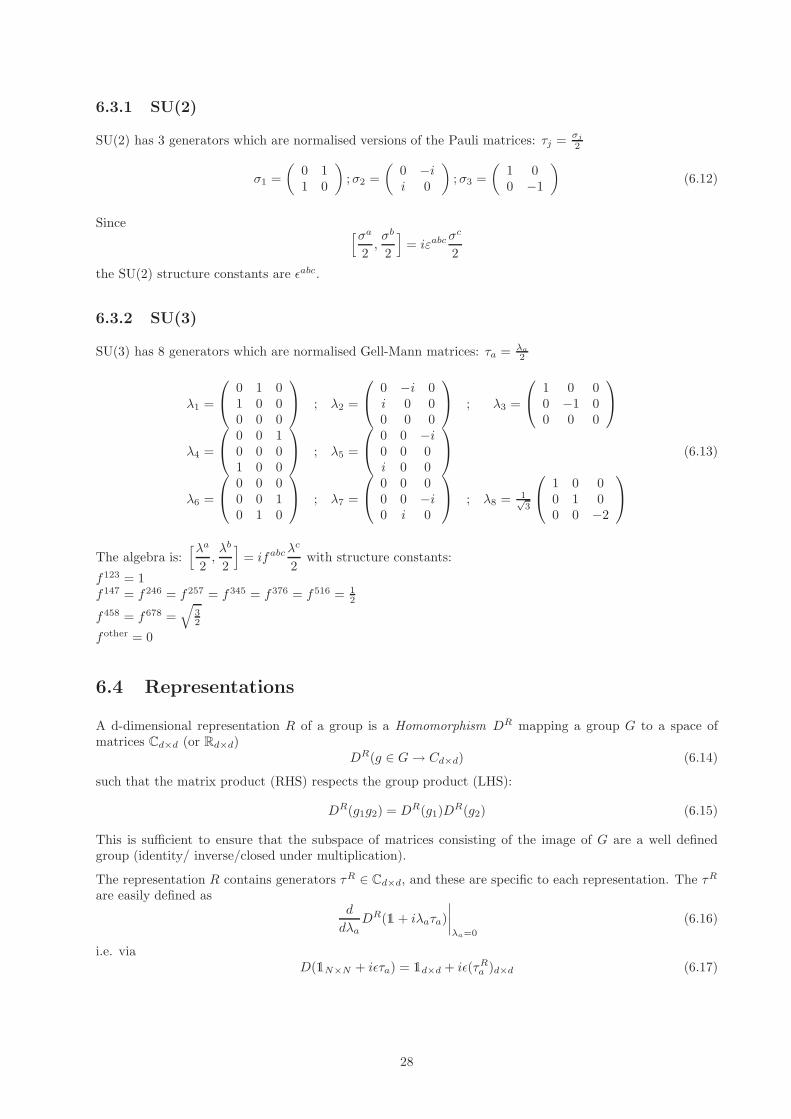
6.3.1 SU(2)

SU(2) has 3 generators which are normalised versions of the Pauli matrices: τj =σj

2

σ1 =

(0 11 0

);σ2 =

(0 −ii 0

);σ3 =

(1 00 −1

)(6.12)

Since [σa

2,σb

2

]= iεabcσ

c

2

the SU(2) structure constants are ǫabc.

6.3.2 SU(3)

SU(3) has 8 generators which are normalised Gell-Mann matrices: τa = λa

2

λ1 =

0 1 01 0 00 0 0

; λ2 =

0 −i 0i 0 00 0 0

; λ3 =

1 0 00 −1 00 0 0

λ4 =

0 0 10 0 01 0 0

; λ5 =

0 0 −i0 0 0i 0 0

λ6 =

0 0 00 0 10 1 0

; λ7 =

0 0 00 0 −i0 i 0

; λ8 = 1√3

1 0 00 1 00 0 −2

(6.13)

The algebra is:[λa

2,λb

2

]= ifabcλ

c

2with structure constants:

f123 = 1f147 = f246 = f257 = f345 = f376 = f516 = 1

2

f458 = f678 =√

32

fother = 0

6.4 Representations

A d-dimensional representation R of a group is a Homomorphism DR mapping a group G to a space ofmatrices Cd×d (or Rd×d)

DR(g ∈ G→ Cd×d) (6.14)

such that the matrix product (RHS) respects the group product (LHS):

DR(g1g2) = DR(g1)DR(g2) (6.15)

This is sufficient to ensure that the subspace of matrices consisting of the image of G are a well definedgroup (identity/ inverse/closed under multiplication).

The representation R contains generators τR ∈ Cd×d, and these are specific to each representation. The τR

are easily defined asd

dλaDR(1 + iλaτa)

∣∣∣∣λa=0

(6.16)

i.e. viaD(1N×N + iǫτa) = 1d×d + iǫ(τR

a )d×d (6.17)

28

6.4.1 Equivalence and reality

Two representations are equivalent if they are related by a unitary basis change

τRa = U−1TR′

a U

Remembering the factor of i in eiΛaτa

, we categorise the reality of a representation R, if it is equivalent toone in which reality of the exponent is:

real if R is the same as its complex conjugate R:

iτRa = −i(τR

a )∗ = iτ Ra

pseudoreal if R is equivalent to its complex conjugate R under basis change:

iτRa = −iV −1(τR

a )∗V = iV −1(τ Ra )∗V

complex if R is inequivalent to its complex conjugate R:

iτ Ra = −i(τR)∗ 6≡ iτR

a

6.4.2 Singlet representation

There is always a very trivial and boring representation of any group. This is called a singlet representation.

D(g) = 1d×d ∀g ∈ G (6.18)

Here, if d = 1 the representation is a mapping to real or complex numbers. If d > 1 the representation is tomatrices, but the singlet image of G consists of only the identity 1 in all cases.

States (i.e. wavefunctions) transformed by this representation not really transformed at all – they areunaltered by the symmetry transformation as it simply multiplies by one. For example, spin-0 states areunaltered by rotations as they have no spin direction that needs to be rotated as the axes change.

6.4.3 Fundamental representation

Dfundamental(g) ≡ SU(N) is the defining, or fundamental, representation.

States transformed by the fundamental D(g) have an index j with N components which are acted upon bymultiplication by this matrix, in the same way that a matrix multiplies a vector.

These states may, of course, have other components α in tensor product with j. The multiplication by D(g)is then of course done for each value of α as one expects of tensors.

For example, we might consider a flavor triplet f ∈ (u, d, s) of Dirac fields with spin index α. A SU(3) flavourbasis rotation ψ′

f ′α = gf ′fψfα is performed for each spin component α. The field ψ is a vector describingeach of the up, down and strange quark spinors.

6.4.4 Adjoint representation

This representation has Dadjoint(g) ∈ C(N2−1)×(N2−1) and is defined by

Recall we introduced the covariant derivative Dµ = ∂µ + ieAµ, transforming as D′µ = gDµg

†.

If the group for g is promoted to a Lie group such as SU(N), then Aµ = Aaµτ

a lies in the Lie Algebra andbecomes a (heavily constrained) complex N ×N matrix.

For now we take g to be a global transformation so that not terms involving derivatives appear, we see that

A′µ → gAµg

†

29

A field transforming like this is said to be in the Adjoint representation.

Viewed from the perspective of the N2−1 real valued coefficents of the generators Aaµ, we can ask how these

components transform.

We may write for an infinitesimal transformation

(Abµ)′τb = (1 + iǫτa)Ac

µτc(1− iǫτa)

= Abµτ

b + iǫ[τa, τc]Acµ

= Abµτ

b + ifacbAbµǫτ

b

= Abµτ

b − ifabcAbµǫτ

b

In terms of the adjoint field components Aaµ the field has been multiplied by the matrix 1(N2−1)×(N2−1) +

i(T a)bc where(T a

adjoint)bc = −ifabc (6.19)

Gluon fields are in the adjoint representation of SU(3), and their transformation can equivalently be viewedin terms of complex 3× 3 or real 8× 8 operations on the Lie Algebra.

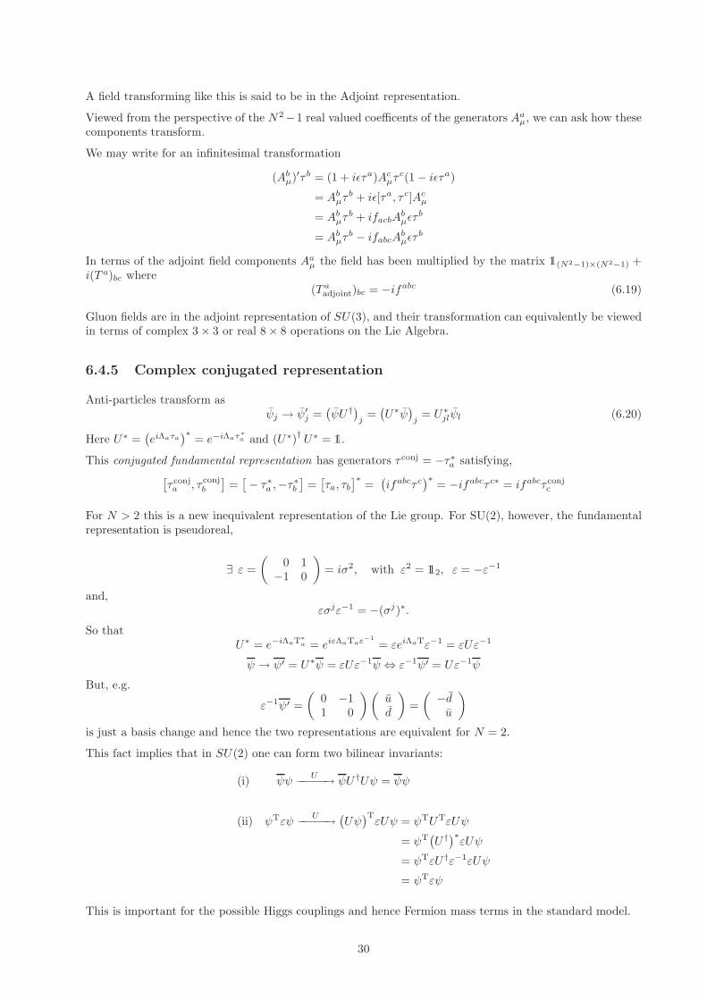
6.4.5 Complex conjugated representation

Anti-particles transform asψj → ψ′

j =(ψU †)

j=(U∗ψ

)j

= U∗jlψl (6.20)

Here U∗ =(eiΛaτa

)∗= e−iΛaτ∗

a and (U∗)† U∗ = 1.

This conjugated fundamental representation has generators τconj = −τ∗a satisfying,[τconja , τconj

b

]=[− τ∗a ,−τ∗b

]=[τa, τb

]∗=(ifabcτc

)∗= −ifabcτc∗ = ifabcτconj

c

For N > 2 this is a new inequivalent representation of the Lie group. For SU(2), however, the fundamentalrepresentation is pseudoreal,

∃ ε =

(0 1−1 0

)= iσ2, with ε2 = 112, ε = −ε−1

and,εσjε−1 = −(σj)∗.

So thatU∗ = e−iΛaT∗

a = eiεΛaTaε−1

= εeiΛaTε−1 = εUε−1

ψ → ψ′ = U∗ψ = εUε−1ψ ⇔ ε−1ψ′ = Uε−1ψ

But, e.g.

ε−1ψ′ =

(0 −11 0

)(ud

)=

(−du

)

is just a basis change and hence the two representations are equivalent for N = 2.

This fact implies that in SU(2) one can form two bilinear invariants:

(i) ψψU−−−−−→ ψU †Uψ = ψψ

(ii) ψTεψU−−−−−→

(Uψ)TεUψ = ψTUTεUψ

= ψT(U †)∗εUψ

= ψTεU †ε−1εUψ

= ψTεψ

This is important for the possible Higgs couplings and hence Fermion mass terms in the standard model.

30

Chapter 7

Analysis of SU(3)

The generators λi can be put in a more useful basis.

I1 = 12λ1 ; U1 = 1

2λ4 ; V1 = 12λ6

I2 = 12λ2 ; U2 = 1

2λ5 ; V2 = 12λ7

I3 = 12λ3 ; U3 = 1

2

(− 1

2λ3 +√

32 λ8

); V3 = 1

2

(12λ3 +

√3

2 λ8

) (7.1)

Commutation relations:

[Ii, Ij ] = iǫijkIk I− spin[Ui, Uj ] = iǫijkUk U− spin[Vi, Vj ] = iǫijkVk V − spin

SU(2) subalgebras

(7.2)

Eq A.19 shows that the topology of SU(2) is simple. Pick a given three dimensional unit vector; this definesa linear combination of Pauli matrices. Traveling in any such direction through the group move simply alonga line combining ident with this matrix with period 2π (and 4π in terms of a rotation angle).

Considering the su(2) sub-algebras of su(3) is more entertaining. I1, I2, U1, U2, V1, V2 look like three pairs ofx − y planes, and are “toroidal”. However, the corresponding z-torii are lie at 60 degrees to each other asI3, U3, V3 are not linearly independent.

Regardless we can define raising and lowering operators as before and investigate the states using ourknowledge of SU(2).

I± = I1 ± iI2 (7.3)

U± = U1 ± iU2 (7.4)

V± = V1 ± iV2 (7.5)

Commutation relations

[I+, I−] = 2I3 (7.6)

[U+, U−] = 2U3 (7.7)

[V+, V−] = 2V3 (7.8)

allow to raise and lower eigenvalues of (λ3, λ8) by amounts

I± ⇒ (δλ3, δλ8) = ±(1, 0) (7.9)

U± ⇒ (δλ3, δλ8) = ±(−1

2,

√3

2) (7.10)

V± ⇒ (δλ3, δλ8) = ±(1

2,

√3

2) (7.11)

These are conceptually just like raising and lower operators for Sz but for SU(3) we have two simultaneouslydiagonalisable “spin” directions.

31

so that all these states also lie on the upper boundary of the allowed quantum numbers of the representation.Generate new sequences V n

− |ψI〉 and V n− |ψI〉.

|ψm〉Ipm|ψm〉

Uqm|ψm〉

Vp−U

q−|ψU〉

Vq−I

p−|ψU〉

Ip−

Uq−

Vp−

Vq−

From these end points apply U− and I− and we have mapped out a boundary, constrained by I ↔ U ↔ Vsymmetry to have three faces of length p+ 1 and three faces of length q + 1.

|ψm〉Ip

m|ψm〉

Uq

m|ψm〉

Vp

−U

q

−|ψm〉

Vq

−I

p

−|ψm〉

Iq

−V

p

−U

q

−|ψm〉

Ip

−

Uq

−

Vp

−

Vq

−

Up

−

Iq

−

Thus we find irregular hexagonal shapes satisfying 120 degree rotation symmetry (p 6= q 6= 0). Special casesof a triangular representation occur when p 6= 0, q = 0 (particles ) or p = 0, q 6= 0 (anti-particles ). Thecase p = q = 0 is the singlet case.

States in the interior may be found by applying raising/lowering operators to states on the boundaries.When both p and q are non-zero, the interior can be shown to have degeneracy raised by one each time westep inwards until a triangular interior is attained. For example, an octet has two states in the central point(π0, η). See Cheng and Li Chapter 4 for details. (At this level of detail, even Cheng and Li starts to get abit sketchy!)

33

The general expression for the number of states in the multiplet is

N = (p+ 1)(q + 1)(p+ q + 2)

2(7.16)

7.1 Young Tableau

We have previously observed that the stepping between irreducible representations, where we find an or-thogonal state to the space just explored by use of ladder operators, follows the symmetrisation and anti-symmetrisation of indices. Young tableau provide a way to automate the generation of possible contractionsof indices, independent of the details of the group we are representing.

If N transforming fields are combined in a multi-particle state, N indices are represented by N boxes. Indicesin the same row represent symmetrisation, while indices in the same column are anti-symmetrised.

These turn out to generate precisely the different irreducible representations of the group.

The technique in combination with the magic formula Eq 7.16 that encodes the structure of SU(3) in termsof integers p and q is sufficient to determine the irreducible representation decomposition and multiplicitiesof arbitrary tensor products of representations of SU(3).

The general form of this formula is known for SU(N), but not necessary to discuss here. The tableau methodcan, in fact, be used to generate both the formula for general SU(N) and also the list of states in eachrepresentation, but this is beyond the scope of this course.

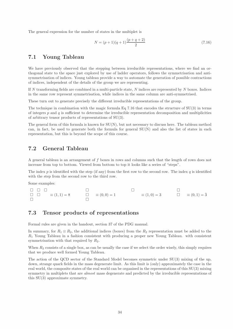
7.2 General Tableau

A general tableau is an arrangement of f boxes in rows and columns such that the length of rows does notincrease from top to bottom. Viewed from bottom to top it looks like a series of “steps”.

The index p is identified with the step (if any) from the first row to the second row. The index q is identifiedwith the step from the second row to the third row.

Some examples:

≡ (1, 1) = 8

≡ (0, 0) = 1

≡ (1, 0) = 3

≡ (0, 1) = 3

7.3 Tensor products of representations

Formal rules are given in the handout, section 37 of the PDG manual.

In summary, for R1 ⊗ R2, the additional indices (boxes) from the R2 representation must be added to theR1 Young Tableau in a fashion consistent with producing a proper new Young Tableau. with consistentsymmetrisation with that required by R2.

When R2 consists of a single box, as can be usually the case if we select the order wisely, this simply requiresthat we produce well formed Young Tableau.

The action of the QCD sector of the Standard Model becomes symmetric under SU(3) mixing of the up,down, strange quark fields in the mass degenerate limit. As this limit is (only) approximately the case in thereal world, the composite states of the real world can be organised in the representations of this SU(3) mixingsymmetry in multiplets that are almost mass degenerate and predicted by the irreducible representations ofthis SU(3) approximate symmetry.

34

Chapter 8

Quark model

Hadrons are particles that feel the strong force; they are classified as:

• spin- 12 ,

32 , . . . baryons: ∼ qqq

• spin-0, 1, . . . mesons: ∼ qq

Prior to 1950’s these consisted of p, n︸︷︷︸spin-1/2

, π±, π0

︸︷︷︸spin-0

where mp ≃ mn ≃ 1 GeV and mπ± ≃ mπ0 ≃ 140 MeV.

We consider p (udu) and n (udd) in SU(2) an “isospin” doublet (fundamental representation 2)

(|p〉 Iz = 1

2|n〉 Iz = − 1

2

).

The three pions are an isospin triplet ( 3 representation from 2⊗ 2 = 1⊕ 3) ):

π+ Iz = +1π0 Iz = 0π− Iz = −1

Around 1950 new particles were observed K±,Σ±, . . . , typically produced in pairs These were “strangely”long lived but heavy particles, and acquired their lifetime because the strange quark could only decay viaweak interactions.

Rationalising the previously “bizarre” spectrum in terms of consituent quarks was a major triumph of grouptheory.

spin 0 spin 12 spin 3

2

K0 ∼ sdπ− ∼ ud...

p ∼ uudn ∼ uddΣ0 ∼ udsΞ− ∼ dss

∆++ ∼ uuuΞ+− ∼ dssΩ− ∼ sss

Observations in the strong interaction

Baryon number (B), Lepton number (L), charge are conserved: they are related to symmetry under globalU(1) transformations:

ψ → ψ′ = eiΛBBeiΛLLeiΛQQψ

We also note

• Q is always measured in terms of electron charge

• anti-particles have opposite B, L, Q quantum numbers

35

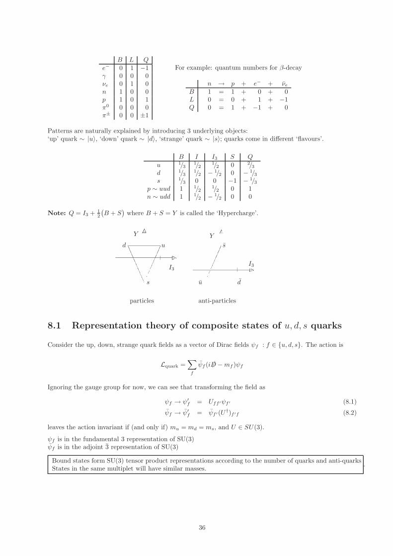
B L Qe− 0 1 −1γ 0 0 0νe 0 1 0n 1 0 0p 1 0 1π0 0 0 0π± 0 0 ±1

For example: quantum numbers for β-decay

n → p + e− + νe

B 1 = 1 + 0 + 0L 0 = 0 + 1 + −1Q 0 = 1 + −1 + 0

Patterns are naturally explained by introducing 3 underlying objects:‘up’ quark ∼ |u〉, ‘down’ quark ∼ |d〉, ‘strange’ quark ∼ |s〉; quarks come in different ‘flavours’.

B I I3 S Qu 1/3

1/21/2 0 2/3

d 1/31/2 − 1/2 0 − 1/3

s 1/3 0 0 −1 − 1/3p ∼ uud 1 1/2

1/2 0 1n ∼ udd 1 1/2 − 1/2 0 0

Note: Q = I3 + 12

(B + S

)where B + S = Y is called the ‘Hypercharge’.

Y

I3

ud

s

particles

Y

I3

du

s

anti-particles

8.1 Representation theory of composite states of u, d, s quarks

Consider the up, down, strange quark fields as a vector of Dirac fields ψf : f ∈ u, d, s. The action is

Lquark =∑

f

ψf (i /D −mf )ψf

Ignoring the gauge group for now, we can see that transforming the field as

ψf → ψ′f = Uff ′ψf ′ (8.1)

ψf → ψ′f = ψf ′(U †)f ′f (8.2)

leaves the action invariant if (and only if) mu = md = ms, and U ∈ SU(3).

ψf is in the fundamental 3 representation of SU(3)ψf is in the adjoint 3 representation of SU(3)

Bound states form SU(3) tensor product representations according to the number of quarks and anti-quarksStates in the same multiplet will have similar masses.

.

36

8.1.1 Meson octet/singlet: 3⊗ 3

These are composite states composed of a quark and anti-quark (mesons) and decompose as follows:

3⊗ 3 =

⊗ =

⊕

(8.3)

= 8⊕ 1 (8.4)

This gives the meson octet with states we call π+, π0, π+,K+,K−, K0,K0, η.

K0 K+

π− π0η π+

K− K0

S

I3

Meson Octet (spin-0)

There is a meson flavor singlet state we call η′

8.1.2 Baryon decuplet/octet 3⊗ 3⊗ 3

Three quark states (baryons) decompose as follows:

3⊗ 3 = ⊗ =

⊕ (8.5)

= 3⊕ 6 (8.6)

Followed by

(3 ⊕ 6)⊗ 3 =

(

⊕

)⊗ (8.7)

=

⊕

⊕

⊕ (8.8)

= 1⊕ 8⊕ 8⊕ 10 (8.9)

This predicts both the baryon decuplet and the octet.

∆∗− ∆∗0 ∆∗+ ∆∗++

Σ∗− Σ∗0 Σ∗+

Ξ∗− Ξ∗0

Ω

S

I3

n ∼ (udd) p ∼ (uud)

Σ− Σ0 Λ Σ+

Ξ− Ξ0

S

I3

Baryon Decuplet (spin-3/2) Baryon Octet (spin-1/2)

37

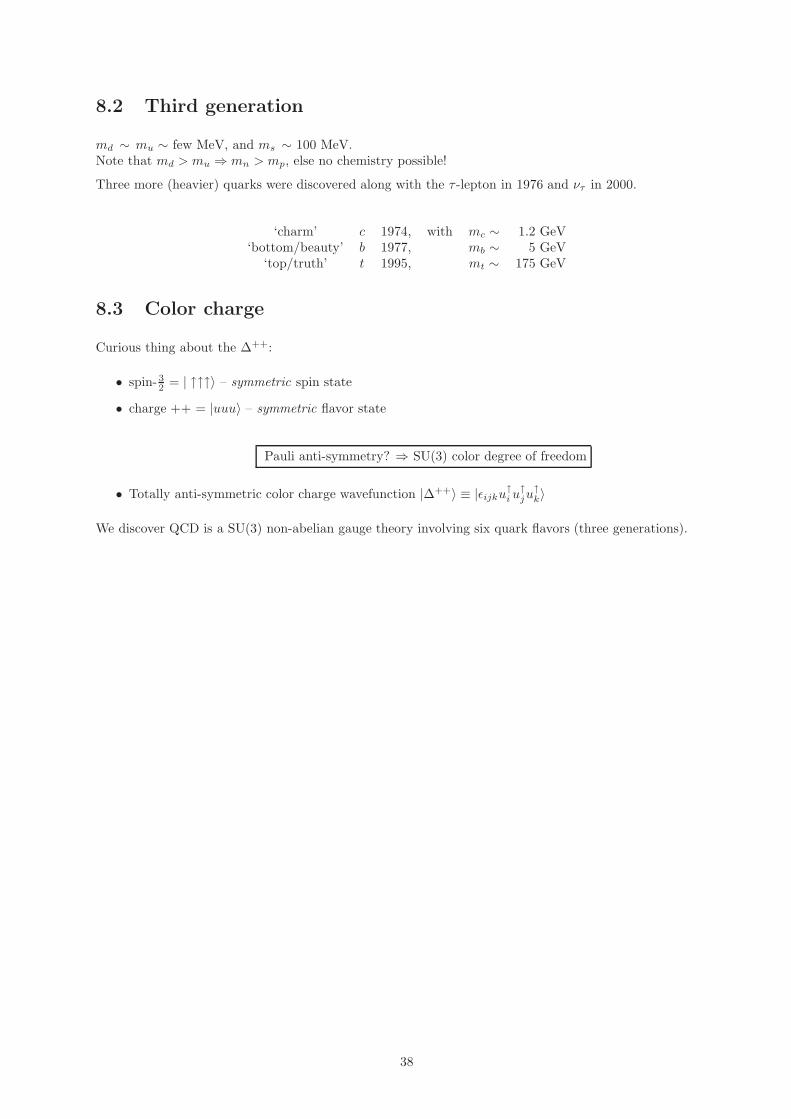
8.2 Third generation

md ∼ mu ∼ few MeV, and ms ∼ 100 MeV.Note that md > mu ⇒ mn > mp, else no chemistry possible!

Three more (heavier) quarks were discovered along with the τ -lepton in 1976 and ντ in 2000.

‘charm’ c 1974, with mc ∼ 1.2 GeV‘bottom/beauty’ b 1977, mb ∼ 5 GeV

‘top/truth’ t 1995, mt ∼ 175 GeV

8.3 Color charge

Curious thing about the ∆++:

• spin- 32 = | ↑↑↑〉 – symmetric spin state

• charge ++ = |uuu〉 – symmetric flavor state

Pauli anti-symmetry? ⇒ SU(3) color degree of freedom

• Totally anti-symmetric color charge wavefunction |∆++〉 ≡ |ǫijku↑i u

↑ju

↑k〉

We discover QCD is a SU(3) non-abelian gauge theory involving six quark flavors (three generations).

38

Chapter 9

SU(N) Yang-Mills theory

Non-abelian gauge theories Yang, Mills (1954)Renormalizability Fadeev, Popov (1969)

SU(N) gauge theory involves a non-abelian gauge transformation group. Non-abelian gauge fields supportself interactions of the gauge bosons. Important realisations of such theories are:

SU(3)C → QCD

SU(2)L ⊗ U(1)→ Weinberg-Salam Model

The Dirac field transforms as a Fermion in the fundamental representation of SU(N). Consider the freeDirac Lagrangian density

L0D

= iψγµ∂µψ −mψψagain with (in a condensed notation)

ψ → ψ′ = Uψ

ψ → ψ′= ψU †

In the fundamental representation the field, ψ, must be a N-vector, with each component being a spinorfield:

ψ ∼

ψ1α

...ψNα

where ψjα has

j as the SU(N) indexα as the spinor index

Examples

SU(3)C ψ =

qr

qb

qg

with q ∈ u, d, s, c, b, t (the six quark ‘flavours’) and ‘r’ = red, ‘b’ = blue, ‘g’ = green (three ‘colours’).

SU(2)L ψL =

(νe

e

)

L

,

(ud

)

L

9.1 SU(N) Lagrangian

Construct Lagrangian density to be invariant under local group transformations g(Λ(x)) ∈ SU(N).

ψ → ψ′ = g(Λ(x))ψ = exp(igNΛa(x)T a)ψ,

where

39

• g(Λ(x)) ∈ SU(N) is an N ×N matrix in the Lie group

• Λa(x)T a is in the Lie algebra su(N) and is a linear combination of generators with a = 1, . . . , N2 − 1

• gN a coupling constant

Construct gauge covariant derivative Dµ introducing N2 − 1 gauge bosons Aµ via “minimal coupling”

∂µ → Dµ = 11∂µ + igNTaAa

µ

Sometimes write T aAaµ as Aµ, and Dµ is matrix-valued in color indices.

[g,Aµ] 6= 0 !!!

For invariance under local transformations we have to require

Dµ → Dµ′ = g(x)Dµg†(x)

As in the Abelian case local group transformations are placed in one-to-one correspondence to gauge trans-formations of gauge fields, and we define the gauge transformation property of Aµ via

Aµ′ = T aA′a

µ = AaµgT

ag† − i

gNg∂µg

†

This results in the required property

∂µ′ + igNAµ

′ =∂µ + igNTaA

′aµ

=g(∂µg†) + gg†∂µ + igNA

aµgT

ag†

=g(∂µ + igNAµ)g†

Using this derivative the Dirac Lagrangian is invariant under local group transformation and is now givenby:

LD =iψγµ(∂µ + igNTaAµa)ψ −mψψ = L0

D + LInt

whereL

Int= gNψγµT

aψAµa = −JaµA

µa

where the N2 − 1 Noether currentsJa

µ = gNψγµTaψ

couple to the gauge bosons.

For the gauge field action we choose our ansatz

Fµν = − i

gN[Dµ, Dν ] where Fµν ≡ T aF aµν .

Evaluating this commutator (where a, b, c = 1, . . . , N2 − 1) we have

[Dµ, Dν ] =[∂µ + igNTaAµ

a, ∂ν + igNTbA

νb]

=[∂µ, ∂ν ] + [∂µ, igNTbAν

b] + [igNTaAµ

a, ∂ν ]

+ [igNTaAµ

a, igNTbAν

b]

=igNTb(∂µAν

b)− igNTbAν

b∂µ+

+ igNTaAµ

a∂ν − igNTa(∂

νAµa)− g2

NAµ

aAν

b[Ta, Tb]

=igNTa(∂µAνa − ∂νAµ

a)− ig2NfabcA

µaA

νbTc

=igNTa(∂µAνa − ∂νAµ

a − gNfabcAµ

bAν

c)

40

Hence we read off thatFµν

a = ∂µAνa − ∂νAµ

a − gNfabcAµ

bAν

c

This new term, −gNfabcAµ

bAν

c, leads to non-trivial interactions in the Yang-Mills theory and to a qualita-tively different behaviour of the corresponding quantum field theory compared to the Abelian case.

Gauge invariance of tr(FµνFµν

)follows from the transformation property of the covariant derivative:

D′µ = gDµg†

which we can readily see

F ′µν=− 1

gN[D′µ, D′ν ]

=− 1

gN[gDµg†, gDνg†]

=− 1

gN

(gDµg†gDνg† − gDνg†gDµg†

)

=− 1

gN

(gDµDνg† − gDνDµg†

)

=− 1

gNg[Dµ, Dν ]g†

=gFµνg†

As a resulttr(F ′µν

F ′µν

)= tr

(FµνFµν

)

This is the gauge invariant expression for the kinetic term.The Yang-Mills Lagrangian is:

LYM

=− 1

2tr(FµνFµν

)where Fµν ≡ F aµνT a

=− 1

2tr(T aT b

)F aµνF b

µν

=− 1

2

(12δab)F aµνF b

µν = −1

4F aµνF a

µν

whereFa

µν = ∂µAaν − ∂νAa

µ − gNfabcAbµAc

µ

Note that the gauge boson acquires self-interaction due to the extra term in the Yang-Mills theory. SinceFµν acquires a term quadratic in the gauge fields, the action acquires additional terms involving three andfour gluon fields. The full Yang-Mills theory including interactions with Dirac Fermions has the Lagrangian:

L = LYM

+ LD

Remarks

• Gauge bosons are charged → only true in the Non-Abelian case!→ self-interactions of the gauge fields and L

YMis already an interacting theory

→ field eqns are nonlinear and difficult to solve (e.g. classical “monopole” and “instanton” solutions).

• No gauge boson mass is allowed because mass terms ∼M2AaµAaµ are not gauge invariant.

• Classical Yang-Mills theory is qualitatively different to the quantum field theory.For instance, g2

N(Q2) −−−−−→Q2→∞

0 where Q is some scale; this is known as asymptotic freedom

• Problem with long-range Yang-Mills interactions:→ in principle, the massless boson has 1/R interaction→ no long range gauge fields are observed apart from the photon (and graviton)→ in nature, Yang-Mills gauge bosons are confined or massive

• gN is the coupling between the fermions and gauge bosons and for self interactions of the gauge bosons→ this property is known as universality of the gauge coupling and can be checked experimentally.

41

Chapter 10

Quantum Chromodynamics

We can now define the QCD sector of the Standard Model as this is an SU(3) gauge theory coupled to sixmassive Dirac Fermions known as quarks.

Quark model and non-abelian g.t. Fritzsch, Gell-Mann, Leutwyler (1972/73)Asymptotic freedom Gross, Politzer, Wilczek (1973)

a.) The quark model has state: ∆++, Ω− → bound states of 3 identical fermions, ∆++ ∼ u↑u↑u↑, whichis not compatible with the exclusion principle.Motivates a distinguishing, extra label organised in an anti-symmetric way called colour:

∆++ ∼∑

i,j,k∈b,r,gu↑iu

↑ju

↑kǫijk

b.) Γ(π0 → γγ)

≈ ≈(

NC

3

)2

If NC = 1 (1 colour), the theoretical prediction for decay rate is a factor of 10 too small (see tutorial).

c.) Quark dynamics must explain why no free quarks (confinement):

→ all hadrons are colour singlets (white)

→ non point-like substructure of hadrons observed in collider experiments ⇒ parton model

→ hadrons made from partons (Feynman, Bjorken 1972 – later indentified as quarks & gluons)

Following success of QED, it was attempted to describe quark dynamics with non-Abelian gauge theory.

⇔ gγ

e−

e+ q

q

QCD was formulated as an SU(3)C gauge theory with quarks (fermions) in the fundamental representation.

L = Lgluon

+ Lquarks

+ Lgauge−fixing

+ Lghost

42

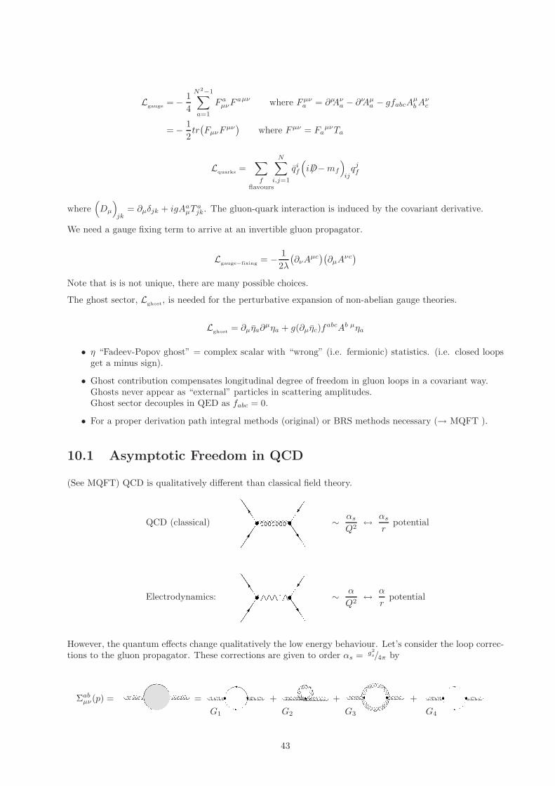
Lgauge =− 1

4

N2−1∑

a=1

F aµνF

aµν where Fµνa = ∂µAν

a − ∂νAµa − gfabcA

µbA

νc

=− 1

2tr(FµνF

µν)

where Fµν = FaµνTa

Lquarks =∑

fflavours

N∑

i,j=1

qif

(iD/−mf

)

ijqjf

where(Dµ

)

jk= ∂µδjk + igAa

µTajk. The gluon-quark interaction is induced by the covariant derivative.

We need a gauge fixing term to arrive at an invertible gluon propagator.

Lgauge−fixing

= − 1

2λ

(∂νA

µc)(∂µA

νc)

Note that is is not unique, there are many possible choices.

The ghost sector, Lghost

, is needed for the perturbative expansion of non-abelian gauge theories.

Lghost

= ∂µηa∂µηa + g(∂µηc)f

abcAb µηa

• η “Fadeev-Popov ghost” = complex scalar with “wrong” (i.e. fermionic) statistics. (i.e. closed loopsget a minus sign).

• Ghost contribution compensates longitudinal degree of freedom in gluon loops in a covariant way.Ghosts never appear as “external” particles in scattering amplitudes.Ghost sector decouples in QED as fabc = 0.

• For a proper derivation path integral methods (original) or BRS methods necessary (→ MQFT ).

10.1 Asymptotic Freedom in QCD

(See MQFT) QCD is qualitatively different than classical field theory.

Electrodynamics: ∼ α

Q2↔ α

rpotential

QCD (classical) ∼ αs

Q2↔ αs

rpotential

However, the quantum effects change qualitatively the low energy behaviour. Let’s consider the loop correc-tions to the gluon propagator. These corrections are given to order αs = g2

s/4π by

Σabµν(p) = = +

G1

+

G2

+

G3 G4

43

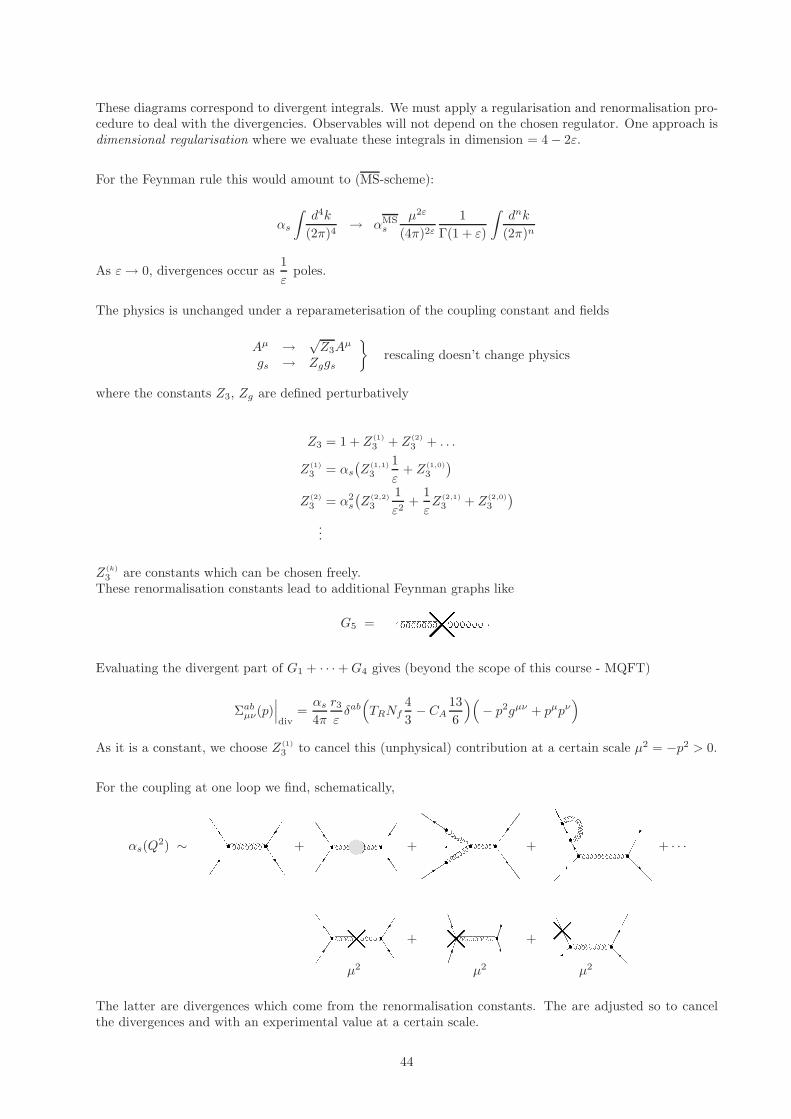
These diagrams correspond to divergent integrals. We must apply a regularisation and renormalisation pro-cedure to deal with the divergencies. Observables will not depend on the chosen regulator. One approach isdimensional regularisation where we evaluate these integrals in dimension = 4− 2ε.

For the Feynman rule this would amount to (MS-scheme):

αs

∫d4k

(2π)4→ αMS

s

µ2ε

(4π)2ε

1

Γ(1 + ε)

∫dnk

(2π)n

As ε→ 0, divergences occur as1

εpoles.

The physics is unchanged under a reparameterisation of the coupling constant and fields

Aµ →√Z3A

µ

gs → Zggs

rescaling doesn’t change physics

where the constants Z3, Zg are defined perturbatively

Z3 = 1 + Z(1)

3 + Z(2)

3 + . . .

Z(1)

3 = αs

(Z(1,1)

3

1

ε+ Z(1,0)

3

)

Z(2)

3 = α2s

(Z(2,2)

3

1

ε2+

1

εZ(2,1)

3 + Z(2,0)

3

)

...

Z(k)

3 are constants which can be chosen freely.These renormalisation constants lead to additional Feynman graphs like

G5 =

Evaluating the divergent part of G1 + · · ·+G4 gives (beyond the scope of this course - MQFT)

Σabµν(p)

∣∣∣div

=αs

4π

r3εδab(TRNf

4

3− CA

13

6

)(− p2gµν + pµpν

)

As it is a constant, we choose Z(1)

3 to cancel this (unphysical) contribution at a certain scale µ2 = −p2 > 0.

For the coupling at one loop we find, schematically,

αs(Q2) ∼ + + + + · · ·

+ +

µ2 µ2 µ2

The latter are divergences which come from the renormalisation constants. The are adjusted so to cancelthe divergences and with an experimental value at a certain scale.

44

αs(Q2) =αs + α2

s

b

ε

(Q2)−ε − α2

s

b

ε

(µ2)−ε

=αs

(1− αsb log

(Q2

µ2

)+O(α2)

)

Quantum corrections in this way lead to a scale-dependent coupling

1

αs(Q2)=

1

αs(µ2)+ b log

(Q2

µ2

); b =

11CA − 4TRNf

12π

This is the renormalised coupling and it depends logarithmically on the scale of the process. The same istrue for QED but b has a different sign.

10.1.1 The logarithmic scale dependence of the strong coupling

The so-called β-function measures the scale dependence of the coupling:

β(αs(Q

2))

=∂

∂ log(Q2)αs = −α2

s(Q2)b

Currently, β is known theoretically to the 4-loop level

∼ β = −α2s

(b+ αsb

′ + α2sb

′′ + α3sb

′′′ + . . .)

At one loop

b =11CA − 4TRNf

12π

The sign of the β-function depends on the particle content of the respective theory. If the number of flavoursin the loop is Nf <

332 ⇒ b > 0. Thus, in the Standard Model, β < 0 (or b > 0). The sign is crucial for the

high energy (ultraviolet) and low energy (infrared) behaviour of the theory.

The running of αs is experimentally confirmed.

45

Ultraviolet behaviour in QCD For b > 0 (β < 0) ⇒ αsQ2→∞−−−−−→ 0. Hence, the quarks feel no gluon

exchange and can be considered as quasi-free particles. This is known as asymptotic freedom (2004 Nobelprize: Gross, Politzer, Wilczek).

Infrared behaviour in QCD For b > 0 implies that there exists a scale, Λ such that αs −−−−−→Q2→Λ2

∞. The

point where the coupling goes to infinity is called the Landau pole, it indicates the strong coupling regime.Of course, perturbation theory itself breaks down long before the Landau pole is reached. Notice that

1

αs(Q2)− 1

αs(Λ2)=

1

αs(Q2)= b log

(Q2

Λ2

)

For Nf = 5, this gives αs(M2Z) = 0.1182± 0.0027 one finds:

Λ = MZe−1/2bαs|M2

Z | ∼ O(200MeV ).

As αs is large at hadronic scale, ∼ 1 GeV , perturbation theory is not applicable. QCD is a stronglyinteracting theory at low energy and most of our calculational tools fail in this regime. This is unfortunate,but also a necessary condition for the theory to have a chance of explaining confinement.

In QED, we have no photon self interaction, and the running is reversed: bQED = bQCD

∣∣∣∣∣CA=0TR=1Nf=1

= − 13π < 0.

QCD

αs

Q2

QED

α

Q2

We see that QCD and QED are qualitatively different from one another with opposite asymptotic behaviour.Quantitative solutions in low-energy QCD are intrinsically difficult. The dynamics is non-perturbative.

Our lack of knowledge of the internal dynamics of the low energy bound states of QCD can be parametrisedusing general functions with the correct allowable Lorentz structure.

These can in some cases be measured in one process and reapplied in another. We shall see an example ofthis with the pion decay constant.

Better yet we can calculated such quantities using non-perturbative numerical methods → Lattice gaugetheory.

46

Chapter 11

Goldstone’s theorem

We now study gauge invariant models with a nontrivial vaccuum structure. Such models display SpontaneousSymmetry Breaking: this means the action is gauge invariant under some symmetry but the ground state(or vaccuum) is not and this breaks the symmetry.

S[φ, ψ, Fµν

]=S[Uφ,Uψ,UFµνU †]

We use 〈· · ·〉 to denote the vacuum expectation value (or vev).A vev for fields with angular momentum would be incompatible with the observed isotropy of space. Forexample, a vev for fermions (→ spin) or gauge fields (→ 〈 ~E〉, 〈 ~B〉)

⇒ 〈ψ〉, 〈Fµν〉 = 0

However a vev for a scalar is allowed〈φ〉 6= 0

We will see below that the Goldstone Theorem implies that there exists a massless mode for each generator Ta

which does not leave the vacuum invariant, Ta〈φ〉 6= 〈φ〉. These massless fields are called Nambu-Goldstonebosons.

Recall that an explicit gauge boson mass term in the Lagrangian is not invariant. In combination with agauge theory, the massless Nambu-Goldstone boson will lead to a massive vector boson (→ Higgs mechanism).A massless gauge boson together with a Nambu-Goldstone boson combines to a massive gauge field. Onemay say that the gauge field acquires a longitudinal component through interaction with the nontrivialvacuum.

Spontaneous Symmetry Breaking (SSB) is not specific to particle physics. Ferromagnets and Superconduc-tors are two other examples.

11.1 SSB in an U(1) scalar field theory

We will see: If the vacuum breaks the symmetry of the theory then a massless mode is created.

Note: As U(1) is isomorphic to SO(2) one can view the model as a so-called SO(2) symmetric σ-model.

φ =1√2

(φ1 + iφ2

) (or φ =

1√2

(φ1

φ2

)for SO(2)

)

L =∂µφ†∂µφ− µ2φ†φ− λ

(φ†φ

)2with λ > 0

=1

2∂µφ1∂

µφ1 +1

2∂µφ2∂

µφ2 −µ2

2

(φ2

1 + φ22

)− λ

4

(φ2

1 + φ22

)2

47

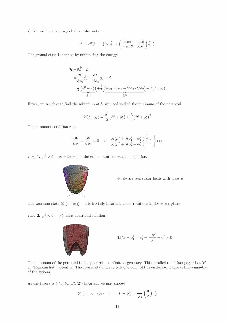
L is invariant under a global transformation

φ→ eiθφ(

or φ→(

cos θ sin θ− sin θ cos θ

)φ)

The ground state is defined by minimising the energy:

H =~π~φ− L

=∂L∂φ1

φ1 +∂L∂φ2

φ2 − L

=1

2

(π2

1 + π22

)︸︷︷︸

≥0

+1

2

(∇φ1 · ∇φ1 +∇φ2 · ∇φ2

)︸︷︷︸

≥0

+V (φ1, φ2)

Hence, we see that to find the minimum of H we need to find the minimum of the potential

V (φ1, φ2) =µ2

2

(φ2

1 + φ22

)+λ

4

(φ2

1 + φ22

)2

The minimum condition reads

∂V

∂φ1=∂V

∂φ2= 0 ⇔ φ1

(µ2 + λ(φ2

1 + φ22)) !

= 0

φ2

(µ2 + λ(φ2

1 + φ22)) !

= 0

(∗)

case 1. µ2 > 0: φ1 = φ2 = 0 is the ground state or vaccuum solution.

φ1, φ2 are real scalar fields with mass µ

The vaccuum state 〈φ1〉 = 〈φ2〉 = 0 is trivially invariant under rotations in the φ1,φ2-plane.

case 2. µ2 < 0: (∗) has a nontrivial solution

2φ∗φ = φ21 + φ2

2 =−µ2

λ= v2 > 0

The minimum of the potential is along a circle→ infinite degeneracy. This is called the “champagne bottle”or “Mexican hat” potential. The ground state has to pick one point of this circle, i.e. it breaks the symmetryof the system.

As the theory is U(1) (or SO(2)) invariant we may choose

〈φ1〉 = 0, 〈φ2〉 = v(

or 〈φ〉 =1√2

(0v

) )

48

Applying a phase transform to the vaccuum we find

eiΛθ〈φ〉 6= 〈φ〉 ⇒ U(1) symmetry “broken”

The physical spectrum is obtained after expanding around the vev of the theory

φ1 = π, φ2 = σ = H + 〈φ2〉 = H + v

where the new fields have

〈π〉 = 0, 〈H〉 = 0

L =1

2∂µπ∂

µπ +1

2∂µH∂

µH − µ2

2

[π2 + (v +H)2

]− λ

4

[π2 + (v +H)2

]2

=1

2∂µπ∂

µπ +1

2∂µH∂

µH − µ2

2

[π2 + v2 + 2vH +H2

]− λ

4

[π2 + v2 + 2vH +H2

]2

Collect the terms with different powers of π, H :

∼ π0, H0 : −µ2

2 v2 − λ

4 v4 irrelevant constant; can’t affect the E.o.M

∼ π0, H1 : −µ2v − λv3 = 0 linear terms give rise to tadpoles,nonexistent in the theory

∼ π2, H0 : −µ2

2 − λ2 v

2 = 0 π’s are massless∼ π0, H2 : µ2 Gives mass: 1

2∂µH∂µH − 1

2m2HH

2

where m2H = −2µ2 > 0

The other terms define the interactions between π,H .We conclude that

• π is a massless spin-zero boson, the Nambu-Goldstone boson

• H is a massive spin-zero boson, the Higgs boson

11.2 Generalisation to SO(N)

~φ =

π1

...πN−1

σ

∈ R

N

This is in the fundamental representation of SO(N) where the generators U ∈ SO(N) are such that UU−1 =11 and detU = 1. There are N(N − 1)/2 generators, all of which are antisymmetric matrices.

U = exp(i

N∑

i<j

ΛijT(ij))∈ SO(N)

where

(T (ij)

)kl

= −i(δikδjl − δilδjk

)

49

The Lagrangian

L =1

2∂µ~φ T∂µ~φ− µ2

2

(~φ T~φ

)− λ

4

(~φ T~φ

)2

is invariant under global SO(N) transformations. For µ2 < 0, V (~φ) is minimal if φiφi = −µ2

λ = v2 > 0, andhence we choose

〈~φ〉 =

0...0v

〈~φ〉 is invariant under SO(N − 1) transformations (generators T (ij) with i < j < k which are defined by

the T (ij)〈~φ〉 = 〈~φ〉). The remaining N − 1 generators T (ik) break the vacuum as T (ik)〈~φ〉 6= 〈~φ〉. There are12 (N(N − 1))− 1

2 (N − 1)(N − 2) = N − 1 broken generatorsWe see that the vev breaks SO(N) spontaneously to SO(N − 1)..

Looking at the spectrum, we find

• πj=1,...,N−1 massless Goldstone bosons

• σ = H + v → H is a massive state with mass M2H = 2λV 2 known as the Higgs boson mass

11.3 Classical Goldstone Theorem

To each generator which breaks the vacuum, i.e. T a〈~φ〉 6= ~0, corresponds a massless field (Nambu-Goldstoneboson).

Proof: We need the definition of the mass matrix in the following:

Mij =∂2V

∂φi∂φj

∣∣∣∣∣~φ=〈~φ〉

The symmetry of the action implies

V (~φ) =V (~φ+ iεaT a~φ) = V (~φ) +∂V

∂φjiεaT a~φ+O(|ε|2)

⇒ ∂V

∂φjT a

jlφl = 0

Applying another derivative on the last line gives

0 =∂

∂φk

( ∂V∂φj

T ajlφl

)∣∣∣∣∣~φ=〈~φ〉

=

(∂2V

∂φk∂φjT a

jlφl +∂V

∂φjT a

jk

) ∣∣∣∣∣~φ=〈~φ〉

and finally one obtaines0 = Mkj T

ajl〈φl〉︸︷︷︸6=~0j

+0 .

If T a is a “broken” generator one has T a〈~φ〉 6= ~0⇒Mkj has a null eigenvector ⇒ null eigenvalues ⇒ massless particle for each such generator. (Note that theeigenvalues of the mass matrix are the particle masses, as the particle are defined as their mass eigenstates.)This completes the proof.

We now combine the concept of a spontaneously broken symmetry with a gauge theory.

50

Chapter 12

Higgs mechanism

The Higgs Mechanism for U(1) gauge theory

Consider

L =(Dµφ∗

)(Dµφ

)− µ2

(φ∗φ

)− λ(φ∗φ

)2 − 1

4FµνFµν

with Dµ = ∂µ + iQAµ and Fµν = ∂µAν − ∂νAµ. Gauge symmetry here means invariance under Aµ →Aµ − ∂µΛ.

case a) unbroken case, µ2 > 0 : V (φ) = µ2(φ∗φ

)+ λ(φ∗φ

)2with a minimum at φ = 0.

The ground state or vaccuum is U(1) symmetric. The corresponding theory is known as Scalar Electrody-namics of a massive spin-0 boson with mass µ and charge Q.

case b) nontrivial vaccuum case

V (φ) has a minimum for 2(φ∗φ

)= −µ2

λ = v2 which gives 〈φ〉 = v√2eiα.

We may choose α = 0 as α is arbitrary but fixed.

eiΛQ〈φ〉 6= 〈φ〉 → SSB

We may parameterise the field in polar coordinates

φ =1√2Reiθ =

1√2

(v +H + i π

)

The kinetic term is

Dµφ =(∂µ + iQAµ

) 1√2Reiθ

=1√2

(∂µR+ iR∂µθ + iQAµR

)eiθ

Dµφ∗ =

1√2

(∂µR− iR∂µθ − iQAµR

)e−iθ

The potential term is

V (φ∗φ) =1

2µ2R2 +

λ

4R4

51

L =1

2

(∂µR∂µR

)+

1

2R2∂µθ∂µθ −

1

2Q2R2AµAµ +QR2Aµ∂

µθ − V (R2)− 1

4FµνFµν

=1

2

(∂µR∂µR

)− V (R2)− 1

4FµνFµν +

1

2Q2R2

(Aµ +

1

Q∂µθ)2

Now we note that the term Aµ + 1Q∂µθ looks like a gauge field transformation. In fact, it can be gauged

away1: Aµ → A′µ = Aµ + 1

Q∂µθ. Now, we see that 〈R〉 = v as R = v +H .

L =1

2

(∂µH∂µH

)− V

((v +H)2

)− 1

4F ′µν

F ′µν −

1

2Q2(v +H)2A′µA′

µ

=1

2

(∂µH∂µH

)− V

((v +H)2

)− 1

4F ′µν

F ′µν −

1

2Q2v2A′µA′

µ −1

2Q2(2vH +H2)A′µA′

µ

In the unbroken case the particle content contained Aµ, a massless gauge boson (2 d.o.f’s) and two massivescalar fields φ1, φ2 (2 d.o.f’s) all in all 4 d.o.f’s.

SSB: After mapping H,π ↔ R, θ it is manifest that θ is a massless Nambu-Goldstone boson that can begauged away; and Aµ is massive with 3 d.o.f’s: 2 transverse + 1 longitudinal. We say that “θ is eaten” bythe gauge field. H is massive: 1 degree of freedom. The number of d.o.f’s (=4) is unchanged.

We see, that the Goldstone boson is absorbed by the gauge boson leading to a longitudinal degree of freedomfor the gauge field. This is called the Higgs mechanism after P. W. Higgs (1964). Ideas along the same linewere developed by Brout, Englert, Hagen and Kibble around the same time.

1This was first noted in condensed matter physics by Anderson. P. W. Higgs applied it to theoretical particle physics.

52

Chapter 13

Electroweak unification

The Standard Model is a gauge theory with the gauge group:

SU(3)C ⊗ SU(2)L ⊗ U(1)Y

It defines the fundamental interaction of Fermions (leptons and quarks), gauge bosons and the Higgs boson.

The electroweak sector SU(2)L⊗U(1)Y is spontaneously broken via the Higgs mechanism. It displays otherodd features.

13.1 Weirdness in the Weak sector

Up to around 1956 it was expected that charge-conjugation (C), parity (P ), and time reversal (T ) were eachsymmetries of nature.

Why?

• A breakage of joint CPT would break Lorentz invariance

• Dirac equation: suggests C should be a good symmetry

• US drives on left, UK drives on right: suggests P should be a good symmetry

• Classical mechanics is reversible: suggests T should be a good symmetry

In 1956 T. D. Lee and C. N. Yang observed while C and P invariance had been rigorously checked experi-mentally for the strong interactions, no such test had been made for weak decays.

Parity and CP violation history

1956 T. D. Lee & C. N. Yang suggest Parity, Charge and CP violation experiments

1957 C.S. Wu et al discover Co60 beta decay has strong parity asymmetry

1957 T.D. Lee & C. N. Yang : two component neutrino theory

1958 Marshak & Sudarshan,Feynman & Gell-Mann : V-A four fermi coupling

1957 Lee and Yang Nobel Prize

1964 Cronin and Fitch discover CP violation in neutral kaon system

1963 Cabbibo quark flavour mixing

c1970 Glashow-Salam-Weinberg Theory unifies electro-weak sector

53

1972 Kobayashi Maskawa

1980 Cronin and Fitch Nobel Prize

2008 Kobayashi-Maskawa-Nambu Nobel Prize

Wu experiment

The Wu experiment placed Co60 in a magnetic field aligning nuclear spinElectrons preferentially emitted in direction opposite to magnetic field→ Parity breaking angular distribution of beta (e−) particles

T. D. Lee and C. N. Yang concluded that the reclusive neutrino always spin aligns with the direction ofpropagation. Breaks parity (defines the sense of a left-handed screw).

The anti-neutrino always spin anti-aligns with the direction of propagation.

Helicity and chirality coincide for massless neutrinos ⇒ V-A current

νγµ(1 − γ5)e

enters the four fermi interaction (Marshak & Sudarshan, Feynman & Gell-Mann).

Model does not violate joint CP :neutrino↔ anti-neutrino and left handed spin ↔ right handed spin

Parity breaking

We have mentioned the V −A weak coupling vertex several times.

Consider an e− + νe → W− transition, where the electron momentum is large and in the z direction. TheW-boson couples to the V-A current

Jµ = uν(p′)γµ(1− γ5)ue(p) =1

2uν(p′)(1 + γ5)γµ(1 − γ5)ue(p)

We take the case ofpµ = (p, pz)

andp′µ = (p′, p′z

The we take χ ∈(

10

),

(01

)as up/down two spinors and our external four spinors are

ue =

(χe

σzχe

)uν =

(χ†

ν ,−χ†νσz

)

We then have

(1− γ5)ue =

((1 − σz)χe

−(1− σz)χe

)uν(1 + γ5) =

(χ†

ν(1− σz),−χ†ν(1− σz)

)

Observe that 12 (1 − σz) =

(1 00 0

)projects out only left handed components. The corresponding W

boson processes for the parity flipped right handed spins do not exist and this mechanism lead to the Wuexperiment asymmetry.

13.2 Glashow-Salam-Weinberg Theory SU(2)L ⊗ U(1)Y

Both Parity violation and CP violation are explained by the unified electro-weak sector, also referred to asGlashow-Salam-Weinberg Theory (c. 1970), Electro-Weak Theory, or Quantum Flavour Dynamics.

54

Electroweak theory describes electromagnetic and weak interactions.The gauge group is spontaneously broken via the Higgs mechanism SU(2)L ⊗ U(1)Y −−−−−−−−→

SSBreakdownU(1)EM

Theory is chirally coupled gauge theory:left handed fields, ψL, φL, transform as SU(2)L doubletsright handed fields, ψR, φR, transform as SU(2)L singlets

ψ L/R=

1

2

(11∓ γ5

)ψ such that Pψ L/R

= ψ R/L

Left-handed doublets are in the fundamental representation of SU(2)L (weak isospin):

(νe

e

)

L

→(ν′ee′

)

L

= eiΛaT a

(νe

e

)

L

eR → e′R = eR (singlet)

(ud

)

L

→(u′

d′

)

L

= eiΛaT a

(ud

)

L

uR → u′R = uR

dR → d′R = dR

Theory does not distinguish between quarks, colour blind

13.2.1 Lagrangian

We can write the theory as the sum of Lagrangian densities:

L = Lgauge

+ LHiggs

+ Lfermion

+ LYukawa

[+Lghost

]

Note that the Yukawa sector, LYukawa, allows for boson and fermion interactions; the “ghost” sector is neededto maintain covariance whilst quantising a non-Abelian gauge theory.

13.2.2 The gauge sector: Lgauge

Electromagnetic interactions are related to an unbroken gauge theory as it contains a massless boson; electriccharge is conserved leaving the photon massless.Weak interactions are short range hence we need SSB to create exchange particle mass

massless ∼ 1

r→ massive ∼ e−mr

r

Glashow, Salam, and Weinberg constructed a Lagrangian which explained all existing data so far.

gauge group: SU(2)L ⊗ U(1)Y

generators: T 1, T 2, T 3

︸︷︷︸weak isospin

Y

gauge coupling: g g′

The Lagrangian may be written as

Lgauge

= −1

4W jµν

W jµν −

1

4BµνBµν

55

where

W jµν =∂µW

jν − ∂νW

jµ − gεjlmW l

µWm

ν j ∈ [1, 2, 3]

Bµν =∂µBν − ∂νBµ the U(1)Y field

This theory describes four massless vector bosons but we need to break this to only one using the Higg’smechanism.

13.2.3 The Higgs sector: LHiggs

We generate gauge boson masses by spontaneous symmetry breakdown:need 1 massless gauge boson (photon) and 3 massive gauge bosons (weak interactions)

Minimal choice: introduce a scalar field as an SU(2) doublet

~φ =1√2

(π1 + iπ2

σ + iπ3

)=

(φ+

φ0

)

where T (~φ) = 12 transforms under the fundamental representation of SU(2)L.

Assign hypercharge: Y (~φ) = 12 .

To make the theory invariant under local transformations, we need

Dµ = ∂µ + ig1

2~σ · ~Wµ

︸︷︷︸SU(2) coupling

+ ig′Y Bµ︸︷︷︸U(1) coupling

The Lagrangian is then

LHiggs

= (Dµ~φ)†(Dµ~φ)− V (~φ†~φ)

where

V (~φ†~φ) = µ2~φ†~φ+ λ(~φ†~φ)2

(It can be shown that globally symmetric SU(2) scalar theory is isomorphic to the SO(4) sigma-model. Seetutorial for more details.)

Note that µ2 < 0 and λ > 0 leads to SSBreakdown.

〈~φ〉 = 1√2

(0v

)with v =

√−µ2

λ

Consider

(T 3 + Y

)︸︷︷︸

Q

〈~φ〉 =[1

2

(1 00 −1

)+

1

2

(1 00 1

)]

︸︷︷︸0

@

1 00 0

1

A

〈~φ〉 ⇒ eiΛQ〈~φ〉 = 〈~φ〉

56

T 1〈~φ〉 = 1

2√

2

(0 1−1 0

)(0v

)=

1√

23

(v0

)6= 〈~0〉

Hence, T 1 is a broken generator. The same is true for T 2 and T 3−Y meaning that we have three Goldstonebosons which we may gauge away. The SU(2)L doublet can be written as (tutorial)

~φ = exp(−i1vT jθj)

1√2

(0

H + v

)= U † 1√

2

(0

H + v

)

The term U † = exp(−i 1vT jθj) looks like a SU(2)L local group element. The Goldstone bosons, θj , play herethe role of the space-time dependent parameters.

Applying the gauge transformation U leads to the so-called unitary gauge:

~φ→ ~φ′ = U~φ =1√2

(0

H + v

)

We obtain

LHiggs

=1

2

[Dµ

(0

H + v

)]†Dµ

(0

H + v

)+ V

(12(H + v)2

)

︸︷︷︸Lquad

We can write

~σ · ~Wµ =σ1W 1µ + σ2W 2

µ + σ3W 3µ =

(W 3

µ W 1µ − iW 2

µ

W 1µ + iW 2

µ −W 3µ

)

Thus in this gauge:

Dµ

(0

H + v

)=(∂µ + i

g

2~σ · ~Wµ + i

g′

21

)(0

H + v

)

=

(0

∂µH

)+ i(g′

2Bµ −

g

2W 3

µ

)( 0v +H

)+ i

g

2

(W 1

µ − iW 2µ

)( v +H0

)

and similarly:

(Dµ

(0

H + v

))†

= (0, ∂µH)− i g2

(W 1

µ + iW 2µ

)(v +H, 0)− i

(g′2Bµ −

g

2W 3

µ

)(0, v +H)

LHiggs =1

2∂µH∂

µH − µ2

2(v +H)

2 − λ

4(v +H)

4+

+g2

8(v +H)2(W 1

µW1µ +W 2

µW2µ) +

1

8

(g′Bµ − gW 3µ)(

g′Bµ − gW 3µ

)(v +H)

2

This Lagrangian defines interaction and mass terms

The charged vector boson masses can be read off directly from

M2W

2(W 1

µW1µ +W 2

µW2µ) =

g2v2

8

((W 1

µ)2 + (W 1µ)2)

leading to

MW± = MW 1,2 =(gv

2

)

57

The interactions of W 1,2 arise through the combinations W±µ = W 2

µ ± iW 2µ , and these linear combinations

are the W+ and W− gauge bosons.

For the quadratic term in the W 3µ, Bµ bosons we find

Lquad =v2

8

(W 3

µ , Bµ

)( g2 −gg′−g′g g′2

)(W 3

µ

Bµ

)

The eigenvalues of the mass matrix are:

λ = 0 λ = g2 + g′2

The mass term is a diagonal quadratic form of the field g′Bµ−gW 3µ , and we find the normalised eigenvectors

are parallel and orthogonal to this

1√g2 + g′2

(−gg′

)1√

g2 + g′2

(g′

g

)

Making the field redefinition,

(W 3

µ

Bµ

)=

(cos θW sin θW

− sin θW cos θW

)(Zµ

Aµ

), sin θW =

g′

(g2 + g′2)1/2

we get

Lquad

=v2

8

(g2 + g′

2)(Zµ

Aµ

)(1 00 0

)(Zµ

Aµ

)

We see that Aµ is massless and that Zµ is a massive vector boson with mass M2Z = g2+g′2

4 v2, and the othermassive state in Higgs sector is the Higgs boson with mass M2

H = −2µ2 = 2λv2.

13.2.4 The fermion sector: Lfermion

Massive Dirac-fermions can be split into left and right-handed chiral components by using projectors PL/R:

ψ = ψL + ψR = PLψ + PRψ , PL/R =1

2

(1∓ γ5

)

In the original formulation of the Standard Model the massless left handed neutrinos had no right-handedpartners. Recently observed neutrino oscillations suggest right-handed neutrinos but we shall stick to theoriginal formulation in the following.

The SU(2)L ⊗ U(1)Y quantum numbers for the fermions are

Leptons T (isospin) Y (hypercharge) T3 Q = T3 + Y

(νe

e

)

L

,

(νµ

µ

)

L

,

(ντ

τ

)

L

1/2 − 1/21/2− 1/2

0−1

eR, µR, τR 0 −1 −1 0

Quarks T (isospin) Y (hypercharge) T3 Q = T3 + Y

(ud′

)

L

,

(cs′

)

L

,

(tb′

)

L

1/21/6

1/2− 1/2

2/3− 1/3

uR, cR, tR 0 2/3 0 2/3

d′R, s′R, b

′R 0 − 1/3 0 − 1/3

58

To give an example for the notation:

ψc=red,f∈1,2L =

(creds′red

)

L

, ψc=blue,f=2R = (d′blue)R

The reason for introducing the primed quark fields q′ in the list will become clear below.

We can now construct the fermion Lagrangian

Lfermion =∑

colours cflavours f

ψ

cf

L iD/ ψcfL + ψ

cf

R iD/ ψcfR

where we have to distinguish the covariant derivative acting on the left fields

Dµ = 1∂µ + ig~σ

2~Wµ + ig′Y Bµ1

from the one acting on the right fields, as the latter do not couple to SU(2)L gauge bosons.

Dµ = ∂µ + ig′Y Bµ

Consider the fermion gauge boson interactions

Lfermion =∑

c,f

(ψ

cf

L i∂/ ψcfL + ψ

cf

R i∂/ ψcfR

)+

g′√2

∑

c,f

ψcfγµPL

(T+W+

µ + T−W−µ

)ψcf

−e∑

c,f

QfψcfA/ψcf −g

2 cos θW

∑

c,f

ψcfγµ(Vf −Afγ5

)ψcfZµ

with Vf = T3 f − 2Qf sin2 θW , Af = T3 f and e =gg′√g2 + g′2

= g sin θW = g′ cos θW is the elementary

charge.

T+ =1

2

((0 11 0

)+ i

(0 −ii 0

))=

(0 10 0

); T− =

(0 01 0

)

Lfermion

is not sufficient to provide mass terms; we need to couple the fermions to the Higgs sector to achievethat.

There are no mass terms because gauge invariance does not allow them as L/R fields cannot be adequatelycombined. For example:

mee =m(ePRe+ ePLe

)

=m(eLeR + eReL

)

=meLeR + Hermitian conjugate

But this is not a gauge invariant term under SU(2)L and hence it is forbidden.

Note that we have used ePR = e†γ0PR = e†PLγ0 = e†P †Lγ0 =

(PLe

)†γ0 = eL

59

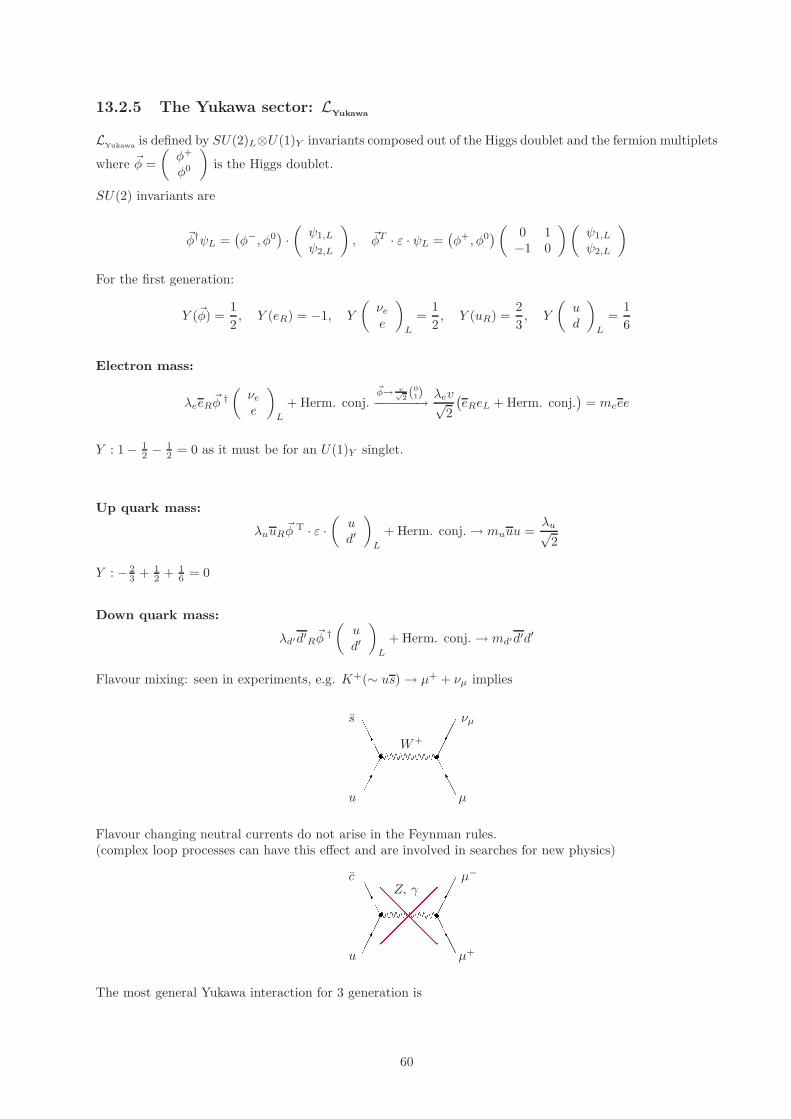
13.2.5 The Yukawa sector: LYukawa

LYukawa is defined by SU(2)L⊗U(1)Y invariants composed out of the Higgs doublet and the fermion multiplets

where ~φ =

(φ+

φ0

)is the Higgs doublet.

SU(2) invariants are

~φ†ψL =(φ−, φ0

)·(ψ1,L

ψ2,L

), ~φT · ε · ψL =

(φ+, φ0

)( 0 1−1 0

)(ψ1,L

ψ2,L

)

For the first generation:

Y (~φ) =1

2, Y (eR) = −1, Y

(νe

e

)

L

=1

2, Y (uR) =

2

3, Y

(ud

)

L

=1

6

Electron mass:

λeeR~φ †(νe

e

)

L

+ Herm. conj.~φ→ v√

2(01)−−−−−−→ λev√

2

(eReL + Herm. conj.

)= meee

Y : 1− 12 − 1

2 = 0 as it must be for an U(1)Y singlet.

Up quark mass:

λuuR~φ T · ε ·

(ud′

)

L

+ Herm. conj.→ muuu =λu√

2

Y : − 23 + 1

2 + 16 = 0

Down quark mass:

λd′d′R~φ†(

ud′

)

L

+ Herm. conj.→ md′d′d′

Flavour mixing: seen in experiments, e.g. K+(∼ us)→ µ+ + νµ implies

s

W+

νµ

u µ

Flavour changing neutral currents do not arise in the Feynman rules.(complex loop processes can have this effect and are involved in searches for new physics)

cZ, γ

µ−

u µ+

The most general Yukawa interaction for 3 generation is

60

LYukawa

= −(eR, µR, τR

)Cl

~φ †·(νe

e

)

L

~φ †·(νµ

µ

)

L

~φ †·(ντ

τ

)

L

+(d′R, s′R, b′R

)Cq

~φ †·(ud′

)

L

~φ †·(cs′

)

L

~φ †·(tb′

)

L

+(uR, cR, tR

)C′

q

~φ T· ε·(ud′

)

L

~φ T· ε·(cs′

)

L

~φ T· ε·(tb′

)

L

+ Herm. conj.

where Cl, Cq, C′q ∈ C3×3.

SU(2)⊗ U(1) invariance seems to allow for generation mixing.

We now have to ask the question how many entries in the matrices are actually physical, means cannot beabsorbed by a redefinition of fields and complex phases.

Consider making a basis change (this does not affect the physics):

eµτ

R

→ U1

eµτ

R

,

uct

R

→ U2

uct

R

,

d′

s′

b′

R

→ U3

d′

s′

b′

R

ψe

ψµ

ψτ

R

→ V1

ψe

ψµ

ψτ

R

,

ψu

ψc

ψt

R

→ V2

ψu

ψc

ψt

R

where U1, U2, U3, V1, V2 ∈ U(3).

We can now use this transformation to reduce the degrees of freedom in Cl, Cq, C′q.

Cl → U †1ClV1, C′

q → U †2C

′qV2, Cq → U †

3CqV2

13.2.6 Simplifications

Recall Hermitian ⇒ diagonalisable: C†C is automaticall Hermitian positive semi-definite with eigenvaluesλ2.

Our matrices C are merely complex and not diagonalisable. However, complex matrix has a singular valuedecomposition

C = UDV †

where U , V are unitary, D is diagonal with elements λ ≥ 0 and λ2 are the eigenvalues of C†C.

Thus we can write

Cl = UlDlV†l Cq = UqDqV

†q Cq′ = Uq′Dq′V †

q′

61

13.2.7 Lepton sector

ChooseU1 = Ul, V1 = Vl ⇒ Cl → Dl = diag(λe, λµ, λτ )

No lepton flavour mixing

Lepton-gauge couplings diagonal in same basis as that with a diagonal mass matrix.

13.2.8 The quark sector

ChooseU2 = Uq′ , V2 = Vq′ ⇒ Cq′ = diag(λu, λc, λt)

But,

Cq → U3UqDqV†q V

†2

is not diagonalisable. We have already chosen V2.

Greatest simplification obtained by taking

U3 = V2VqU†q ⇒ Cq = V DqV

†

where V = V2Vq is the unitary Cabibbo-Kobyashi-Maskawa matrix (1973).

By using our free choice for U2 and V2 to diagonalise C′q we see that Cq can in general not be diagonalised

at the same time. We are left with a unitary rotation which acts on the d, s, b quarks.

There is still some freedom that allows us to restrict V ∈ U(3) further. We are free to apply a phasetransformation on ψL/R since the wave functions are defined up to a global phase.

V →

e−iϕ1 0 00 e−iϕ2 00 0 e−iϕ3

V

eiχ1 0 00 eiχ2 00 0 eiχ3

Consider first the case of two generations:

V2 gens. =

(e−i(ϕ1−χ1)V11 e−i(ϕ1−χ2)V12

e−i(ϕ2−χ1)V21 e−i(ϕ2−χ2)V22

)

The three phase differences can be chosen such that: V11 ≥ 0, V12 ≥ 0, V21 ≤ 0.The 4th phase is fixed as ϕ2 − χ2 = (ϕ2 − χ1) + (ϕ1 − χ2)− (ϕ1 − χ1). This gives

V =

(V11 V12

−|V21| eiρV22

), V † =

(V11 −|V12|V21 e−iρV22

)

as V ∈ U(2)⇒ V V † = 11⇒

V 211 + V 2

21 = 1

−V11|V21|+ V12V22e−iρ = 0

|V21|2 + V 222 = 1

To fulfill these three conditions we need ρ = 0, an imaginary phase is not allowed. Hence

V11 = V22 = cos θC

V11 = |V21| = sin θC

θC ∈ [0,

π

2] is called the Cabibbo angle

62

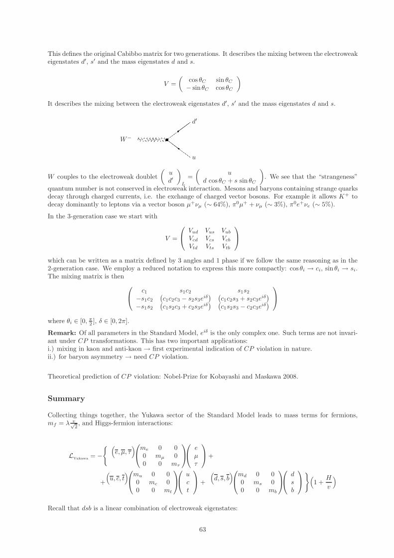
This defines the original Cabibbo matrix for two generations. It describes the mixing between the electroweakeigenstates d′, s′ and the mass eigenstates d and s.

V =

(cos θC sin θC

− sin θC cos θC

)

It describes the mixing between the electroweak eigenstates d′, s′ and the mass eigenstates d and s.

W−

d′

u

W couples to the electroweak doublet

(ud′

)

L

=

(u

d cos θC + s sin θC

). We see that the “strangeness”

quantum number is not conserved in electroweak interaction. Mesons and baryons containing strange quarksdecay through charged currents, i.e. the exchange of charged vector bosons. For example it allows K+ todecay dominantly to leptons via a vector boson µ+νµ (∼ 64%), π0µ+ + νµ (∼ 3%), π0e+νe (∼ 5%).

In the 3-generation case we start with

V =

Vud Vus Vub

Vcd Vcs Vcb

Vtd Vts Vtb

which can be written as a matrix defined by 3 angles and 1 phase if we follow the same reasoning as in the2-generation case. We employ a reduced notation to express this more compactly: cos θi → ci, sin θi → si.The mixing matrix is then

c1 s1c2 s1s2−s1c2

(c1c2c3 − s2s3eiδ

) (c1c2s3 + s2c3e

iδ)

−s1s2(c1s2c3 + c2s3e

iδ) (

c1s2s3 − c2c3eiδ)

where θi ∈ [0, π2 ], δ ∈ [0, 2π].

Remark: Of all parameters in the Standard Model, eiδ is the only complex one. Such terms are not invari-ant under CP transformations. This has two important applications:i.) mixing in kaon and anti-kaon → first experimental indication of CP violation in nature.ii.) for baryon asymmetry → need CP violation.

Theoretical prediction of CP violation: Nobel-Prize for Kobayashi and Maskawa 2008.

Summary

Collecting things together, the Yukawa sector of the Standard Model leads to mass terms for fermions,mf = λ v√

2, and Higgs-fermion interactions:

LYukawa = − (

e, µ, τ)me 0 00 mµ 00 0 mτ

eµτ

+

+

(u, c, t

)mu 0 00 mc 00 0 mt

uct

+

(d, s, b

)md 0 00 ms 00 0 mb

dsb

(

1 +H

v

)

Recall that dsb is a linear combination of electroweak eigenstates:

63

dsb

︸︷︷︸mass eigenstates

= V

d′

s′

b′

︸︷︷︸e.w. eigenstates

We see that the Yukawa sector contains 9 masses + 3 angles + 1 phase = 13 parameters. The parametersof the flavour sector have to be fixed by experiment.

13.3 Feynman Rules of fermion, gauge and Yukawa sectors

∼ ieQfγµA

qf

qf

∼ −ig

2√

2γµ(1 − γ5)

(V †)

ffW

qf

qf

∼ −ig2 cos θW

γµ(Vf −Afγ5)Z

qf

qf

∼ −imf

v =−igmf

2MWH

qf

qf

∼ i

−gµν +

pµpν

M2V

p2 −M2V + iδ

µ ν

The massive gauge boson propagator is given in the unitary gauge. In this gauge no Goldstone bosons arepresent. This is the standard choice for tree level computations.

64

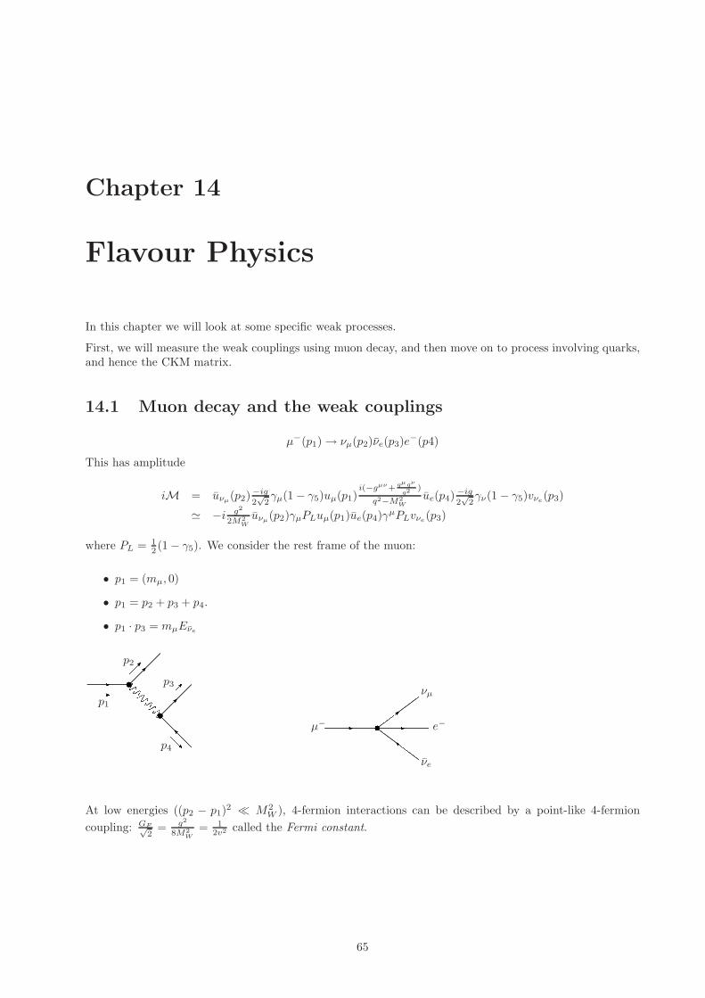
Chapter 14

Flavour Physics

In this chapter we will look at some specific weak processes.

First, we will measure the weak couplings using muon decay, and then move on to process involving quarks,and hence the CKM matrix.

14.1 Muon decay and the weak couplings

µ−(p1)→ νµ(p2)νe(p3)e−(p4)

This has amplitude

iM = uνµ(p2)

−ig

2√

2γµ(1− γ5)uµ(p1)

i(−gµν+ qµqν

q2 )

q2−M2W

ue(p4)−ig

2√

2γν(1 − γ5)vνe

(p3)

≃ −i g2

2M2W

uνµ(p2)γµPLuµ(p1)ue(p4)γ

µPLvνe(p3)

where PL = 12 (1− γ5). We consider the rest frame of the muon:

• p1 = (mµ, 0)

• p1 = p2 + p3 + p4.

• p1 · p3 = mµEνe

p1

p2

p3

p4

µ− e−

νµ

νe

At low energies ((p2 − p1)2 ≪ M2

W ), 4-fermion interactions can be described by a point-like 4-fermion

coupling: GF√2

= g2

8M2W

= 12v2 called the Fermi constant.

65

14.1.1 Measuring the Fermi constant

Note that:(χγµPLφ)† = φ†P †

Lγ†µγ

†0χ

= φ†γ0γ0PLγ0γ0γ†µγ0χ

= φPRγµχ= φγµPLχ

Thus

|M|2 = g4

4M4W

g4

4M4W

[uνµ

(p2)γµPLuµ(p1)ue(p4)γµPLvνe

(p3)] [uµ(p1)γµ′PLuνµ

(p2)vνe(p3)γ

µ′PLue(p4)

]

∑spins

|M|2 = 12

g4

4M4W

Tr/p2γµPL/p1γµ′PLTr/p3γ

µPL/p4γµ′

PL

= 12

g4

4M4W

TrPL/p2γµ/p1γµ′TrPL/p3γ

µ/p4γµ′

Recall:tr(γµγνγργσ

)= 4(gµνgρσ − gµρgνσ + gµρgνσ)

tr(γ5γ

µγνγργσ)

= −4iǫµνρσ

ǫµνρσǫµναβ = −2(δραδ

σβ − δ

ρβδ

σα

)

Thus,TrPL/p2

γµ/p1γµ′ = 2[p2µp1µ′ + p2µ′p1µ − p1 · p2gµµ′ − 2iǫµµ′αβ ]

and similar for p3, p4, leading to

∑spins

|M|2 = 12

g4

4M4W

4[p2µp1µ′ + p1µp2µ′ − (p1 · p2)gµµ′ − iǫµµ′αβp

α2 p

β1

]

×[pµ3p

µ′

4 + pµ4p

µ′

3 − (p3 · p4)gµµ′ − iǫµµ′ρδp3ρp4δ

]

= 12

g4

M4W

[2(p2 · p3)(p1 · p4) + 2(p2 · p4)(p1 · p3)− ǫµµ′αβǫ

µµ′ρδpα2 p

β1p3ρp4δ

]

= 12

g4

M4W

[2(p2 · p3)(p1 · p4) + 2(p2 · p4)(p1 · p3)− 2(p2 · p3)(p1 · p4) + 2(p2 · p4)(p1 · p3)]

= 2g4

M4W

(p2 · p4)(p1 · p3)

This is a useful worked example of performing traces with the γ5 that arises in W and Z vertex rules.

The three body phase space integral to work out the decay width Γ is beyond the scope of the course, butfor completeness can be found in appendix B. This obtains

Γ =(

mµgMW

)4mµ

6144π3

Inserting the experimental mass mµ = 105MeV, lifetime τµ = 2.19703µs⇒ Γ = ~/τ = 2.99× 10−10eV , andwe obtain

GF =

(g

MW

)2 √2

8= 1.166× 10−5(GeV )−2

With the measured MW = gv2 = 80.4GeV we can also determine the weak coupling constant g ∼ 0.653, and

the Higgs VEV v = 246 GeV.

14.2 CKM constraints

Quark flavour mixing is an active research topic– CKM parameters are some of the least well known fundamental constants.– search for possible new physics– LHCb, Babar, Belle, KTEV, NA48, + other experiments.

The CKM matrix is often written in terms of the Wolfenstein parametrisation:

66

V =

Vud Vus Vub

Vcd Vcs Vcb

Vtd Vts Vtb

=

1− λ2

2 λ Aλ3(ρ+ iη)

−λ 1− λ2

2 Aλ2

Aλ3(1− ρ− iη) −Aλ2 1

This parametrisation describes a unitary matrix up to terms of O(λ4).

As V V † = 11 there are 9 relations, for example

V ∗ubVud + V ∗

cbVcd + V ∗tbVtd = 0 ⇔ 1 +

V ∗tbVtd

V ∗cbVcd︸︷︷︸∈C

+V ∗

ubVud

V ∗cbVcd︸︷︷︸∈C

= 0

⇔(1, 0)

+(x2, y2

)+(x1, y1

)= 0

We can identify these as vectors in the complex plane forming a unitary triangle:

(ρ, η)

x2, y2 x1, y1

1, 0

Different experimental measurements measure different combinations of CKM matrices. These measurementscan be turned into constraints on the vertex of this unitarity triangle and these overlayed, and the present(2010) state of the art is shown below (actually, a subset of the constraints):

!

"

"

dm#

K$

K$

sm# & dm#

SLub

V

% &ubV

'sin 2

(excl. at CL > 0.95)

< 0'sol. w/ cos 2

"

'!

(

-0.4 -0.2 0.0 0.2 0.4 0.6 0.8 1.0

)

0.0

0.1

0.2

0.3

0.4

0.5

0.6

0.7

excluded area has CL > 0.95

ICHEP 10

CKMf i t t e r

Hadronic matrix elements

Converting measurements into CKM constraints normally involves some theoretical input to remove theeffects of the hadrons that contained the quarks participating in a process.

Make progress using non-perturbative parameters/functions constrained only by Lorentz symmetry.– Calculate them with Lattice QCD– Obtain them from fits to data

We will consider the three key classes of process presently contributing to CKM constraints: Leptonic decays,Semi-leptonic decays and neutral meson mixing.

67

14.3 Leptonic decays

We do not understand an initial pion in terms of quark momentum distributions. Fourier transforming thetwo quark fields in Jλ(V − A) = uγλ(1 − γ5)d entering Lint

Fermiwill not help us.. Rather, parametrise pion

matrix element of Jλ(V −A) in terms of non-perturbative decay constant

〈π+(p)|Jλ(V −A)〉ifπpλ

This gives an effective pion-W vertex

fπg

2√

2Vudπ

+W+µ p

µ

With Feynman rule fπg

2√

2Vudp

µ

The decay is then given by

iM = Vudfπmπ

(g

2√

2

)2 −g00 +m2

π

M2W

m2π −M2

W

uνe(p2)γ0(1− γ5)ve(p1) (14.1)

≃ VudfπmπGF√

2uνe

(p2)γ0(1− γ5)ve(p1) (14.2)

Thus

Σspins|M|2 =

(Vudfπmπ

GF√2

)2

Tr/p2γ0(1− γ5)/p1

γ0(1− γ5)

=

(Vudfπmπ

GF√2

)2

2Tr/p2γ0(1 − γ5)/p1

γ0

=

(Vudfπmπ

GF√2

)2

82p0

1p02 − pµ

1p2µ

=

(Vudfπmπ

GF√2

)2

8p01p

02 + p

1· p

2

(14.3)

This can be combined with the Lorentz invariant phase space, which we integrate in spherical polar coordi-nates (

∫dΩ = 4π) to obtain the width

∫dΓ =

2

mπ(VudfπmπGF )2

∫d3p1

(2π)3d3p2

(2π)31

2Ee

1

2Eν

[EeEν + p

1· p

2

](2π)4δ(mπ − Ee − Eν)δ3(p

1+ p

2)

=1

2mπ(VudfπGF )2

∫d3p1

(2π)32πδ(mπ − Ee − Eν)

[1− p2

1

EeEν

]

=mπ

2π(VudfπGF )2

∫dpp2δ(mπ − Ee − p)

[1− p

Ee

](14.4)

Where we use Ee =√m2

e + p2 and Eν = p. We note that after integrating the delta function will imposeconservation of energy, and constrain p:

mπ =√m2

e + p2 + p,

p =m2

π −m2e

2mπ=

1

2mπ(1− m2

e

m2π

)

and also √m2

e + p2 − p =m2

e

mπ

We can change variables to u = p+√m2

e + p2 ; du = dp u√m2

e+p2, and so

∫dΓ =

mπ

2π(VudfπGF )

2(mπ

2

)2(

1− m2e

m2π

)21

mπ(√m2

e + p2 − p) (14.5)

=mπ

8π(VudfπGF )2m2

e

(1− m2

e

m2π

)2

(14.6)

68

This decay rate vanishes asme → 0. This is a result of helicity suppression - angular momentum conservationcancels the amplitude in the massless limit when helicity (spin orientation) and chirality coincide. The resultof this is that the decay through the more massive muon channel dominates.

Given Γµ = 2.53× 10−8 MeV, mµ = 106 MeV, mπ = 139.5 MeV, and GF = 1.166× 10−5(GeV)2 we find

Vudfπ ≃ 128MeV

14.3.1 Neutral pion decay

Neutral pion decay is an electromagnetic decay process mediated via the Adler-Bell-Jackiw anomaly in QED.You don’t need to understand what the anomaly is, but it is important to know that there is a spectacularlysuccessful consistency check that the same measured pion decay constant explains both weak decay of chargedpions and electromagnetic decays of neutral pions.

See tutorial:

We obtained fπ ≃ 130MeV

Thus Vud ≃ 1.

Radiative corrections must be included to be more precise than this.

Note the same pion decay constant can be calculated from first principles using Lattice QCD to a precisionof a few percent.

14.4 Semi-leptonic decays

Flavour changing semi-leptonic meson decays are the mesonic analogue of nuclear beta decay, and give goodaccess to elements of the CKM matrix connecting the quark flavours in the initial and final states.

Transition CKM elementK → πeν Vus

B → πeν Vub

B → Deν Vcb

D → Keν Vcs

D → πeν Vcd

e.g. charged kaon decay:

K+ → π0 + e+ + νe

su→ uu+W− → uu+ e+ + νe

K−

π0

e−Vus

u

s

u

ν

W−

Again the unknown kaon and pion internal structure is a theoretical barrier, and we proceed by consideringthe general Lorentz allowed structure for the matrix element of the V − A current to which the W− bosoncouples:

〈π(pπ)|Jµ(V −A)|K(pK)〉 = f+(q2)(pK + pπ)µ + f−(q2)(pK − pπ)µ

Where q2 = (pK − pπ)2, and the decay amplitude is then

iM = Vus

(g

2√

2

)2 [f+(q2)(pK + pπ)µ + f−(q2)(pK − pπ)µ

] −gµν + qµqν

M2W

q2 −M2W

uνe(p2)γν(1− γ5)ve(p1)(14.7)

≃ VusGF√

2

[f+(q2)(pK + pπ)µ + f−(q2)(pK − pπ)µ

]uνe

(p2)γµ(1− γ5)ve(p1) (14.8)

69

Measured lifetime can determine the product GFVusf+(q2).

In order to extract the fundamental constant properly, Vus a non-perturbative theoretical calculation off+(q2 = 0) is required.

However, in the limit ms = mu vector current conservation constrains f+(q2 = 0) = 1. K → π and B → Dare not far from this limit, and we we only make a 4% error by taking f+(q2 = 0) = 1.

With this approximation the experimental decay rate to this channel gives

Vus = 0.211(1)

When recent lattice results for the form factor f+(q2) are used

Vus = 0.2249(14)

Similarly Vcb, and Vub can be found from semileptonic B-decays. Vub requires additional theoretical input(e.g. Lattice QCD) on form factors. We can form

Ru =|Vub||Vud||Vcb||Vcd|

= (1− λ2

2)|ρ+ iη| = |

(ρ, iη

)|

Where ρ = (1− λ2

2 )ρ, and η = (1 − λ2

2 )η.

This constrains the vertex of the unitarity triangle on a circle centered at the origin and radius Ru.

14.5 Neutral meson mixing and CP violation

The Cronin and Fitch experiment (BNL) produced and studied neutral kaons:

|K0〉 ≡ ds |K0〉 ≡ sd CP |K0〉 = −|K0〉 CP |K0〉 = −|K0〉

In the absence of mixing, the time evolution of |K0〉 is

|K0(t)〉 = e−iHt|K0(t)〉 H = M − iΓ2

where M is the mass, and Γ is the decay width of the K0. Similar formula apply for K0.

States mix (oscillate) under weak interaction

If SM preserves CP then SM eigenstates should be CP eigenstates

Physical state CP eigenstate CP lifetime

|KS〉 |K1〉 = |K0〉−|K0〉√2

+1 ( → ππ ∼ 10−10 s)

|KL〉 |K2〉 = |K0〉+|K0〉√2

-1 (→ πππ ∼ 5× 10−8 s)

mK = 495 Mev and mπ = 140 Mev ⇒ due to phase space expect

• |KS〉 ∼ |K1〉 decays rapidly to CP = +1 |ππ〉 state.

• |KL〉 ∼ |K2〉 decays slowly to CP = −1 |πππ〉 state.

Cronin and Fitch found |KL〉 decays at a low rate to ππ ⇒WRONG CP state– manifested as two exponential modes in ππ deposition– ππ production found “at wrong end of detector”

70

Theoretical treatment

K0K0

W+

u, c, t

u, c, t

ds

d s

W−

K0 K0

s

d

u, c, t u, c, t

W−

W+

d

s

Neutral kaon mixing is mediated by box diagrams, for example the left graph is:

iM =∑f,f ′

g4

64 (V ∗dfVfs)(V

∗df ′Vf ′s)I(mf ,mf ′)

I(mf ,mf ′) =∫d4k

vdγµ(1−γ5)(/k−mf )γν(1−γ5)us

k2−m2f

× udγν′(1−γ5)(/k−mf′ )γµ′ (1−γ5)vs

k2−m2f′

×gµµ′− kµkµ′

M2W

k2−M2W

gνν′− kν kν′

M2W

k2−M2W

• Loop integral is convergent →∫

d4kk6

• In mu = mc = mt = mq limit, →(∑

f V∗dfVsf

)(∑f ′ V ∗

df ′Vsf ′)I(mq,mq)

Unitarity gives∑

f V∗dfVsf = 0 → known as (Glashow-Iliopoulos-Maiani) GIM suppression mechanism

GIM correctly predicted (1970) charm quark mass ∼ 1.2 GeV before discovery (1974).

• As eiδ in UT, amplitude is not purely real

14.5.1 Wigner Weisskopf Hamiltonian

With flavour mixing we must consider a matrix QM system:

ψ(t) =

(|K0(t)〉)|K0(t)〉)

)i ddtψ(t) = Hψ

where the Hamiltonian is

H = M − i12Γ =

(M11 − i 12Γ11 M12 − i 12Γ12

M21 − i 12Γ21 M22 − i 12Γ22

)

where since M and Γ must have real positive eigenvalues they are Hermitian matrices. M describes theoscillation betweenK0 and K0, while Γ describes the decay of the system into ππ and πππ states. Hermiticityimplies M21 = M∗

12 and Γ21 = Γ∗12. CPT invariance implies that M11 = M22 = M , and Γ11 = Γ22 = Γ.

Thus a convenient notation is

H =

(M − i 12Γ M12 − i 12Γ12

M∗12 − i 12Γ∗

12 M − i 12Γ

)=

(A αβ A

)

Where A,α, β ∈ C. Eigenvalues can be found easily

det

(A− λ αβ A− λ

)= 0 → λ = A±

√αβ

and the eigenstates are a|K0〉+ b|K0〉 where a(A− λ) + bα = 0, and so

b

a= ±

√β

α

Introduce a parameter ǫ and define normalised eigenstates

KL,S = (1+ǫ)|K0〉±(1+ǫ)|K0〉√2(1+|ǫ|2)

KS = K1+ǫK2√1+|ǫ|2

KL = K2+ǫK1√1+|ǫ|2

71

Where

1− ǫ1 + ǫ

=

√β

α=

√M∗

12 − i 12Γ∗12

M12 − i 12Γ12

The eigenvalues contain a propagating real mass, and an imaginary decay exponent:

λL,S = A±√αβ = M ±ℜ

√(M12 − i

1

2Γ12)(M∗

12 − i1

2Γ∗

12)− i1

2(Γ∓ 2ℑ

√(M12 − i

1

2Γ12)(M∗

12 − i1

2Γ∗

12)

The mixing terms between K0 and K0 create both a mass difference and a lifetime difference1.

∆MK ≃ 2ℜM12

∆ΓK ≃ 2ℜΓ12

14.5.2 Time dependent mixing and mass difference

The B-factories (BaBar and Belle) pair produce B0 and B0 mesons in an entangled quantum state.

CP violating state mixing is tiny in the B system: we can write

|B0〉 = 1√2

(|B1〉+ |B2〉)∼ 1√

2(|BL〉+ |BH〉)

|B0〉 = 1√2

(|B1〉 − |B2〉)∼ 1√

2(|BL〉 − |BH〉)

|BL〉 = 1√2

(|B0〉+ |B0〉

)

|BH〉 = 1√2

(|B0〉 − |B0〉

)

When the first of a coherent pair decays, the flavour state becomes definite (EPR).

Consider first decays as B0 ⇒ the other meson is then pure B0 at this proper time:

ψ(τ = 0) = 1|B0〉+ 0|B0〉 =1√2

(|BL〉+ |BH〉)

Ignoring decays, the subsequent time evolution is

ψ(τ) =1√2

(|BL〉eiMLτe−

12ΓLτ + |BH〉eiMHτe−

12 ΓHτ

)(14.9)

= eiMτe−12Γτ 1√

2

(|BL〉e−i 1

2 ∆Mτe−14∆Γτ + |BH〉ei 1

2∆M τe14∆Γτ

)(14.10)

=1

2eiMτ e−

12Γτ

((e−i 1

2∆M τe−14∆Γτ + ei 1

2 ∆Mτe14∆Γτ )|B0〉

+ (e−i 12∆M τe−

14∆Γτ − ei 1

2 ∆Mτe14∆Γτ )|B0〉

)(14.11)

• The flavour state of the meson oscillates in real time.

• But b→ s (or b→ c), and b→ s (or b→ c)

• Distinguish by looking at the semi-leptonic decay probabilitiesB0 → K+ B0 → K− B0 → D+ B0 → K−

• The B-mesons are moving and the decays of K+ or K− have oscillating spatial structure

Decay probability determined by:

PB0

(τ) = |〈B0|ψ(τ)〉|2 =1

4e−Γτ

[e

12∆γτ + e−

12∆γτ + ei∆M τ + e−i∆Mτ

]=

1

2e−Γτ

[cosh

1

2∆γτ + cos∆Mτ

]

1making use of the experimental observation ǫ ≃ 10−3 and so ℑM12,ℑΓ12 ≪ ℜM12ℜΓ12 givingq

(M12 − i 12Γ12)(M∗

12 − i 12Γ∗

12) ≃ ℜM12 − i 12ℜΓ12

72

and

P B0

(τ) = |〈B0|ψ(τ)〉|2 =1

2e−Γτ

[cosh

1

2∆γτ − cos∆Mτ

]

Note that PB0

(τ = 0) = 1 and P B0

(τ = 0) = 0.

-5 0 5

Evts. / 0.4 ps 200

-5 0 5

Evts. / 0.4 ps 200

tags0B

tags0 B

a)

-5 0 5

Raw asym.

-0.5

0

0.5

-5 0 5

Raw asym.

-0.5

0

0.5 b)

-5 0 5

Evts. / 0.4 ps

100

-5 0 5

Evts. / 0.4 ps

100 tags0B

tags0 B

c)

-5 0 5

Raw asym.

-0.5

0

0.5

-5 0 5

Raw asym.

-0.5

0

0.5 d)

Such measurements of oscillations in the B-system lead to a constraint on the angle sin 2β of the UT triangle.

14.5.3 Indirect CP violation

If the CKM matrix were purely real, then ǫ = 0, and the eigenstates KL,S are the CP eigenstates K1,2.

We find the imaginary phase in the CKM matrix is of huge importance – then β 6= α and the physicaleigenstates are not CP eigenstates and lead to CP violation:

indirect via K1(CP = 1)→ ππ(CP = 1) because |KL〉 ∼ |K2〉+ ǫ|K1〉

direct via |K2〉(CP = −1)→ ππ(CP = 1)

73

Here we only consider indirect CP violation:

KL ∼ ǫK1 + K2

O(ǫ)fast→ ππ O(1)

slow→ πππKS ∼ K1 + ǫK2

O(1)fast→ ππ O(ǫ)

slow→ πππ

PS195

Preliminary

The experimental measure for indirect CP violation is the amplitude ratio

ǫK =A(KL → ππ)

A(KS → ππ)

We require a theoretical determination of M12. The integrals I(mf ,mf ′) can be performed and we find 2

2mKM∗12 =

G2F

16π2M2W

[λ2

cS0(xc, xc)2λcλtS0(xc, xt)λ2tS0(xt, xt)

]

× 〈K0|sγµ(1− γ5)dsγµ(1− γ5)d|K0〉

Here xf =mf

mWand S0(xf , xf ′) are known as Inami-Lim functions. CP violation arises from the imaginary

part of M12. Sinceλt = V ∗

tsVtd = −A2λ5(1 − ρ− iη)the λ2

t piece gives a constraint of the form:

η(1− ρ) = constant

i.e. a hyperbola constraint with pole at ρ = 1.

The non-perturbative hadronic matrix element BK

〈K0|sγµ(1− γ5)dsγµ(1− γ5)d|K0〉 =8

3BKF

2Km

2K

is a theoretical input to determining this constant from the experimental measurement of ǫK .

2using V ∗

usVud = −V ∗

cs − VcdV ∗

tsVtd and mu ∼ 0

74

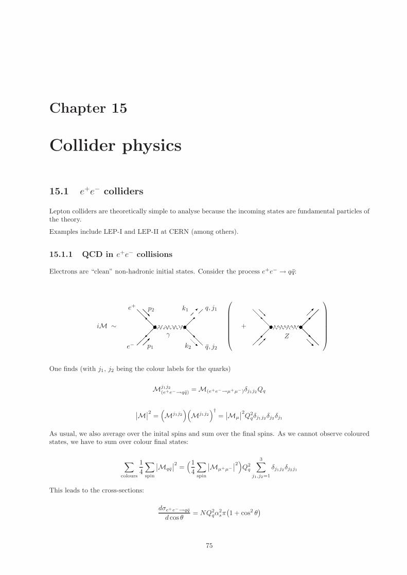
Chapter 15

Collider physics

15.1 e+e− colliders

Lepton colliders are theoretically simple to analyse because the incoming states are fundamental particles ofthe theory.

Examples include LEP-I and LEP-II at CERN (among others).

15.1.1 QCD in e+e− collisions

Electrons are “clean” non-hadronic initial states. Consider the process e+e− → qq:

iM ∼

+

Zγ

e−

e+ q, j1

q, j2p1

p2

k2

k1

One finds (with j1, j2 being the colour labels for the quarks)

Mj1j2(e+e−→qq) =M(e+e−→µ+µ−)δj1j2Qq

∣∣M∣∣2 =

(Mj1j2

)(Mj1j2

)†=∣∣Mµ

∣∣2Q2qδj1j2δj2δj1

As usual, we also average over the inital spins and sum over the final spins. As we cannot observe colouredstates, we have to sum over colour final states:

∑

colours

1

4

∑

spin

∣∣Mqq

∣∣2 =(1

4

∑

spin

∣∣Mµ+µ−∣∣2)Q2

q

3∑

j1,j2=1

δj1j2δj2j1

This leads to the cross-sections:

dσe+e−→qq

d cos θ= NQ2

qα2sπ(1 + cos2 θ

)

75

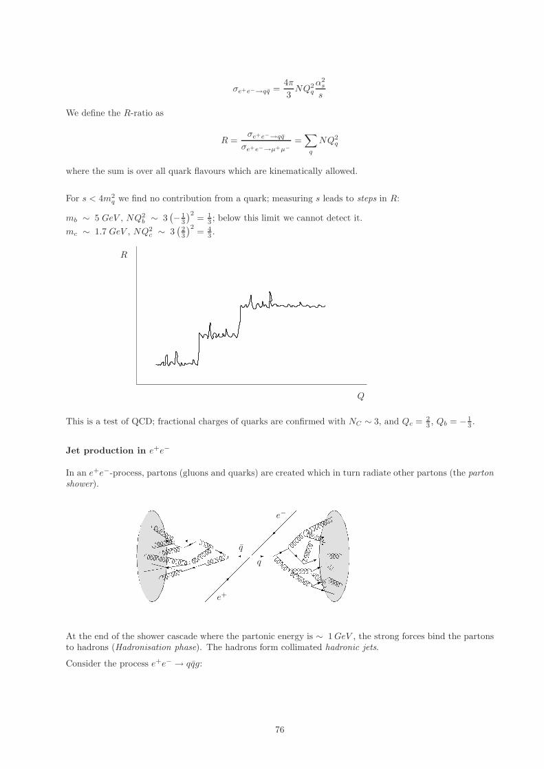
σe+e−→qq =4π

3NQ2

q

α2s

s

We define the R-ratio as

R =σe+e−→qq

σe+e−→µ+µ−=∑

q

NQ2q

where the sum is over all quark flavours which are kinematically allowed.

For s < 4m2q we find no contribution from a quark; measuring s leads to steps in R:

mb ∼ 5 GeV , NQ2b ∼ 3

(− 1

3

)2= 1

3 ; below this limit we cannot detect it.

mc ∼ 1.7 GeV , NQ2c ∼ 3

(23

)2= 4

3 .

R

Q

This is a test of QCD; fractional charges of quarks are confirmed with NC ∼ 3, and Qc = 23 , Qb = − 1

3 .

Jet production in e+e−

In an e+e−-process, partons (gluons and quarks) are created which in turn radiate other partons (the partonshower).

e−

e+

q

q

At the end of the shower cascade where the partonic energy is ∼ 1GeV , the strong forces bind the partonsto hadrons (Hadronisation phase). The hadrons form collimated hadronic jets.

Consider the process e+e− → qqg:

76

iM ∼ + γγ

e−

e+

p1

p2

e−(p1, s1) + e+(p2, s2)→ q(k1, r1, j1) + q(k2, r2, j2) + g(k3, σ, α)

The colour factor, T aj1j2 .

Summation over the final state colours:

N2−1∑

α=1

N∑

j1,j2=1

T aj1j2T

aj2j1 =

N2−1∑

a,b

δab(tr[T aT b]

)

=N2−1∑

a,b

δabTRδab

=N2 − 1

2= NCf where Cf =

N2 − 1

2N

1

4

∑

s1,s2

∑

r1,r2

∑

colours

∣∣M∣∣2 =

(4πα

)2(4παs

)Q2

qNCf

(t211 + t212 + t221 + t222

ss13s23

)

tij =(pi − kj

)2i ∈ 1, 2, j ∈ 1, 2, 3

sij =(ki + kj

)2i, j ∈ 1, 2, 3

p1 =√

s2

(1, 0, 0, 1

), p2 =

√s

2

(1, 0, 0,−1

)→ ~k1 + ~k2 + ~k3 = 0; the vectors must lie in a plane.

Experimentally, we expect to see a plane with 3 jet events.

quark jet

anti-quark jet

gluon jet

The observation of such 3-jet events confirmed the existence of the gluon.

77

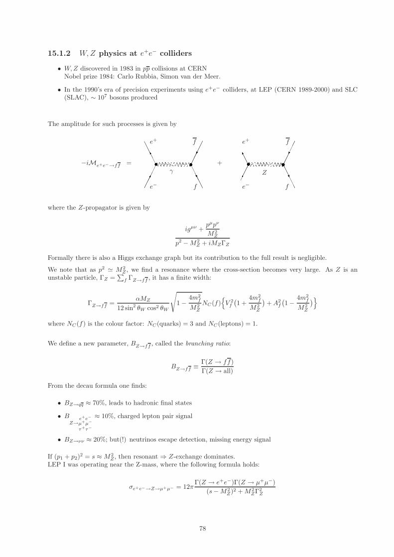
15.1.2 W, Z physics at e+e− colliders

• W,Z discovered in 1983 in pp collisions at CERNNobel prize 1984: Carlo Rubbia, Simon van der Meer.

• In the 1990’s era of precision experiments using e+e− colliders, at LEP (CERN 1989-2000) and SLC(SLAC), ∼ 107 bosons produced

The amplitude for such processes is given by

−iMe+e−→ff = +γ Z

e+

e−

e+

e−

f

f

f

f

where the Z-propagator is given by

igµν +pµpν

M2Z

p2 −M2Z + iMZΓZ

Formally there is also a Higgs exchange graph but its contribution to the full result is negligible.

We note that as p2 ≃ M2Z , we find a resonance where the cross-section becomes very large. As Z is an

unstable particle, ΓZ =∑

f ΓZ→ff , it has a finite width:

ΓZ→ff =αMZ

12 sin2 θW cos2 θW

√

1−4m2

f

M2Z

NC(f)V 2

f

(1 +

4m2f

M2Z

)+A2

f

(1−

4m2f

M2Z

)

where NC(f) is the colour factor: NC(quarks) = 3 and NC(leptons) = 1.

We define a new parameter, BZ→ff , called the branching ratio:

BZ→ff ≡Γ(Z → ff)

Γ(Z → all)

From the decau formula one finds:

• BZ→qq ≈ 70%, leads to hadronic final states

• BZ→

e+e−

µ+µ−

τ+τ−

≈ 10%, charged lepton pair signal

• BZ→νν ≈ 20%; but(!) neutrinos escape detection, missing energy signal

If (p1 + p2)2 = s ≈M2

Z , then resonant ⇒ Z-exchange dominates.LEP I was operating near the Z-mass, where the following formula holds:

σe+e−→Z→µ+µ− = 12πΓ(Z → e+e−)Γ(Z → µ+µ−)

(s−M2Z)2 +M2

ZΓ2Z

78

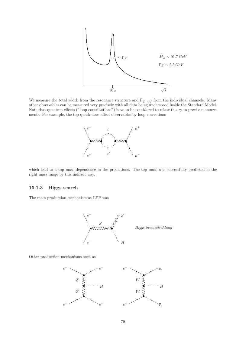
√s

↔ ∼ ΓZ

MZ

MZ ∼ 91.7GeV

ΓZ ∼ 2.5GeV

We measure the total width from the resonance structure and ΓZ→ff from the individual channels. Manyother observables can be measured very precisely with all data being understood inside the Standard Model.Note that quantum effects (”loop contributions”) have to be considered to relate theory to precise measure-ments. For example, the top quark does affect observables by loop corrections

e+

e− t

t′

µ+

µ−

which lead to a top mass dependence in the predictions. The top mass was successfully predicted in theright mass range by this indirect way.

15.1.3 Higgs search

The main production mechanism at LEP was

ZHiggs bremsstrahlung

e+

e−

Z

H

Other production mechanisms such as

e−

e+

e−

e+

H

Z

Z

e−

e+

νe

νe

H

W

W

79

are negligible at LEP.

σe+e−→ZH is sizeable if√s ≥MZ +MH . LEP II found that for

√s ≤ 208GeV ; MH ≥ 114.4GeV ; this is

the experimental lower bound for the Higgs boson.

The Higgs boson is present at the loop level even if not directly detectable. The preferred Higgs mass valueto fit the data implies that MH should be less than about 200 GeV, else radiative corrections induce adiscrepancy to the measured observables.

∼ log(M2H)

If the Standard Model is correct, we expect that the Higgs mass is in the window114.4 GeV < MH < 200 GeV.

15.2 (Large) Hadron colliders

15.2.1 Parton model and proton structure functions

80

Appendix A

Representations of SU(2) and spin

This revision chapter may be insultingly simple and obvious. It will likely be not included or only skimmedin the lectures.

On the other hand, if it is not obvious it may be very useful background reading. I wrote this chapter lastyear after students requested extra help connecting group theory to flavour SU(3) and the Quark Model.

Please feel free to use your judgement.

Recall systems of two or more spin 12 particles have state that is a tensor product.

| ↑〉 → | ↑↑〉| ↓〉 | ↓↑〉

| ↑↓〉| ↓↓〉 (A.1)

Recall the spins can be coupled to formSpin Sz

1 -1,0,10 0

We will consider this coupling in a more group-theoretic fashion to (hopefully) make connection with thelanguage of the Standard Model lectures in a familiar context.

For absolute clarity, please note the tensor product is important. The resulting four states is the product2× 2, not sum 2 + 2. For example, combining three particles yields 23 = 8 states (not 6!).

| ↑〉 → | ↑↑↑〉| ↓〉 | ↓↑↑〉

| ↑↓↑〉| ↓↓↑〉| ↑↑↓〉| ↓↑↓〉| ↑↓↓〉| ↓↓↓〉 (A.2)

These can be comined by pairing the first two as above

(s = 1 ; sz ∈ −1, 0, 1s = 0 ; sz ∈ 0

)⊗(s = 1

2 ; sz ∈ − 12 ,

12

)→

s = 32 ; sz ∈ − 3

2 ,− 12 ,

12 ,

32

s = 12 ; sz ∈ − 1

2 ,12 (1⊗ 1

2 )s = 1

2 ; sz ∈ − 12 ,

12 (0⊗ 1

2 )

(A.3)

81

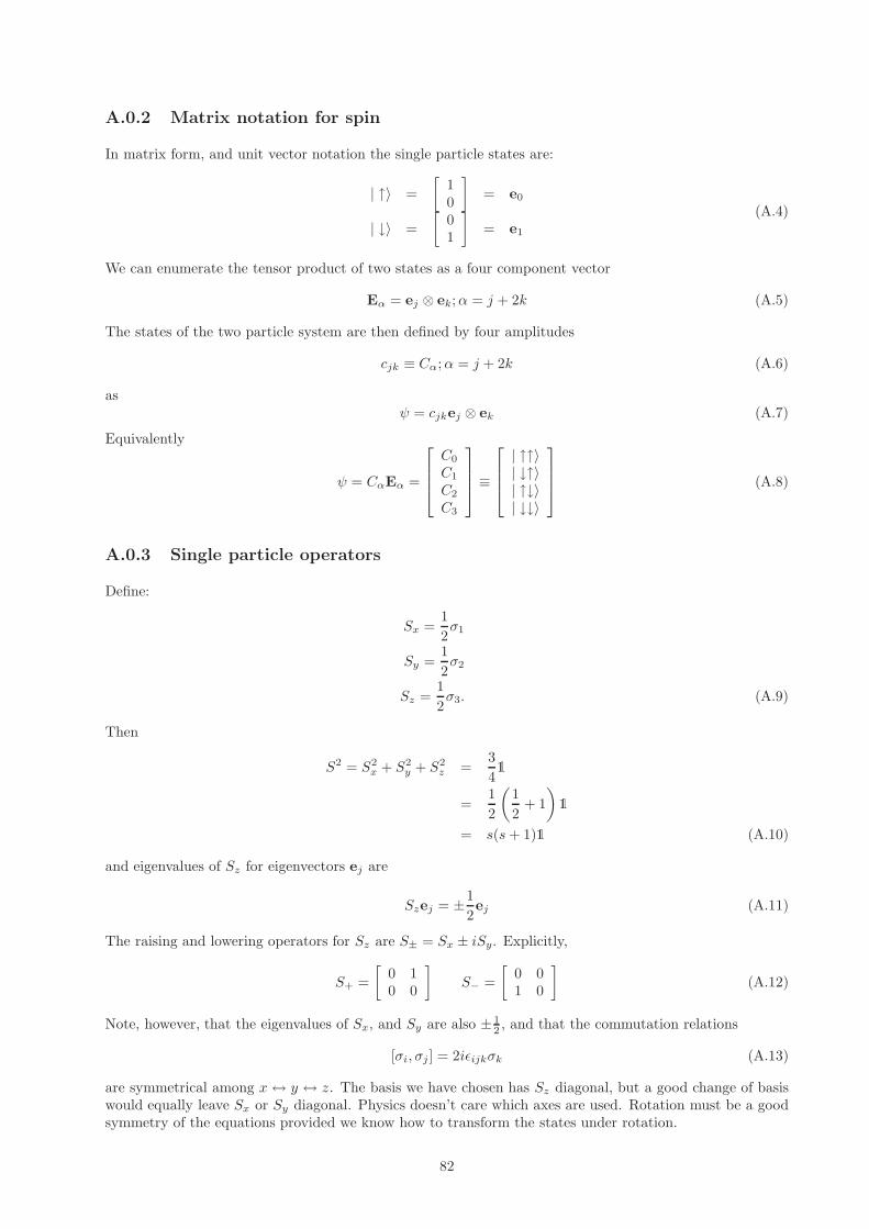
A.0.2 Matrix notation for spin

In matrix form, and unit vector notation the single particle states are:

| ↑〉 =

[10

]= e0

| ↓〉 =

[01

]= e1

(A.4)

We can enumerate the tensor product of two states as a four component vector

Eα = ej ⊗ ek;α = j + 2k (A.5)

The states of the two particle system are then defined by four amplitudes

cjk ≡ Cα;α = j + 2k (A.6)

asψ = cjkej ⊗ ek (A.7)

Equivalently

ψ = CαEα =

C0

C1

C2

C3

≡

| ↑↑〉| ↓↑〉| ↑↓〉| ↓↓〉

(A.8)

A.0.3 Single particle operators

Define:

Sx =1

2σ1

Sy =1

2σ2

Sz =1

2σ3. (A.9)

Then

S2 = S2x + S2

y + S2z =

3

41

=1

2

(1

2+ 1

)1

= s(s+ 1)1 (A.10)

and eigenvalues of Sz for eigenvectors ej are

Szej = ±1

2ej (A.11)

The raising and lowering operators for Sz are S± = Sx ± iSy. Explicitly,

S+ =

[0 10 0

]S− =

[0 01 0

](A.12)

Note, however, that the eigenvalues of Sx, and Sy are also ± 12 , and that the commutation relations

[σi, σj ] = 2iǫijkσk (A.13)

are symmetrical among x↔ y ↔ z. The basis we have chosen has Sz diagonal, but a good change of basiswould equally leave Sx or Sy diagonal. Physics doesn’t care which axes are used. Rotation must be a goodsymmetry of the equations provided we know how to transform the states under rotation.

82

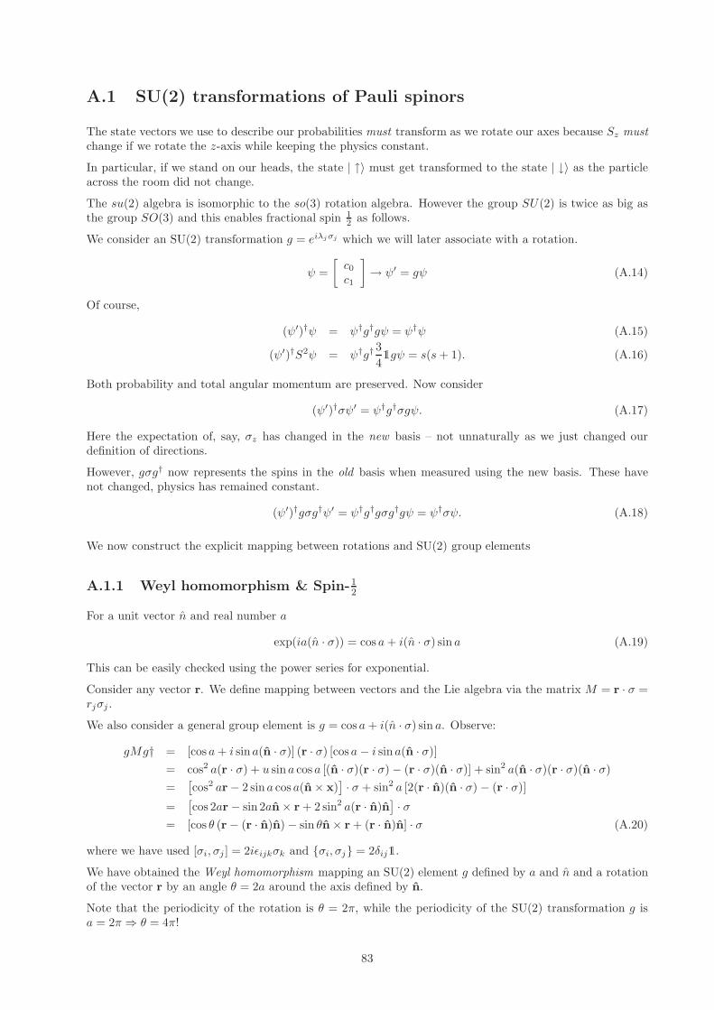
A.1 SU(2) transformations of Pauli spinors

The state vectors we use to describe our probabilities must transform as we rotate our axes because Sz mustchange if we rotate the z-axis while keeping the physics constant.

In particular, if we stand on our heads, the state | ↑〉 must get transformed to the state | ↓〉 as the particleacross the room did not change.

The su(2) algebra is isomorphic to the so(3) rotation algebra. However the group SU(2) is twice as big asthe group SO(3) and this enables fractional spin 1

2 as follows.

We consider an SU(2) transformation g = eiλjσj which we will later associate with a rotation.

ψ =

[c0c1

]→ ψ′ = gψ (A.14)

Of course,

(ψ′)†ψ = ψ†g†gψ = ψ†ψ (A.15)

(ψ′)†S2ψ = ψ†g†3

41gψ = s(s+ 1). (A.16)

Both probability and total angular momentum are preserved. Now consider

(ψ′)†σψ′ = ψ†g†σgψ. (A.17)

Here the expectation of, say, σz has changed in the new basis – not unnaturally as we just changed ourdefinition of directions.

However, gσg† now represents the spins in the old basis when measured using the new basis. These havenot changed, physics has remained constant.

(ψ′)†gσg†ψ′ = ψ†g†gσg†gψ = ψ†σψ. (A.18)

We now construct the explicit mapping between rotations and SU(2) group elements

A.1.1 Weyl homomorphism & Spin-12

For a unit vector n and real number a

exp(ia(n · σ)) = cos a+ i(n · σ) sin a (A.19)

This can be easily checked using the power series for exponential.

Consider any vector r. We define mapping between vectors and the Lie algebra via the matrix M = r · σ =rjσj .

We also consider a general group element is g = cos a+ i(n · σ) sin a. Observe:

gMg† = [cos a+ i sina(n · σ)] (r · σ) [cos a− i sina(n · σ)]

= cos2 a(r · σ) + u sina cos a [(n · σ)(r · σ)− (r · σ)(n · σ)] + sin2 a(n · σ)(r · σ)(n · σ)

=[cos2 ar− 2 sina cos a(n× x)

]· σ + sin2 a [2(r · n)(n · σ) − (r · σ)]

=[cos 2ar− sin 2an× r + 2 sin2 a(r · n)n

]· σ

= [cos θ (r− (r · n)n)− sin θn× r + (r · n)n] · σ (A.20)

where we have used [σi, σj ] = 2iǫijkσk and σi, σj = 2δij1.

We have obtained the Weyl homomorphism mapping an SU(2) element g defined by a and n and a rotationof the vector r by an angle θ = 2a around the axis defined by n.

Note that the periodicity of the rotation is θ = 2π, while the periodicity of the SU(2) transformation g isa = 2π⇒ θ = 4π!

83

Both the element 1 and −1 of SU(2) correspond to the same rotation by 2π.

Recall, for orbital angular momentum L = n continuous rotation by 2π causes the spherical harmonics to passthrough 1 precisely n times, and there to be 2n changes of sign. Under these rules the Weyl homomorphismcorresponds to fractional spin n = 1

2 in terms of orbital angular dependence.

States transformations under SU(2) can be thought of as a multi-branched function of rotations. For thereasonable and continuous choice of following these branches:

Rotations by 2π produce −1, while rotations by 4π produce 1: like a Moebius strip you have to rotate aroundtwice to get back to where you started.

The kernel of a homomorphism H is the set of group elements that map to the identity in the image group.Here KerH = 1,−1 ≡ Z2.

The co-sets of KerH within SU(2) form a group SU(2)/Z2. This factored group is isomorphic to SO(3).

A.2 SU(2) transformations of multi-particle states

Recall three spin 12 particles formed one s = 3

2 and two s = 12 multiplets. By multiplets we mean a family

of states differing in Sz

A.2.1 Different multiplets do not mix

Note that that S2 cannot be changed by an SU(2) transformation. In fact the two s = 12 do not mix with

each other because one was symmetric and the other anti-symmetric under interchange of first two particles.This will be seen to be an important and general feature.

s = 32 sz = (− 3

2 ,− 12 ,

12 ,

32 ) different sz’s in same multiplet mix under rotation

s = 12 sz = (− 1

2 ,12 ) different sz’s in same multiplet mix under rotation

Thus, 12 ⊗ 1

2 ⊗ 12 has an SU(2) representation of the form:

D3particle8×8 (g) =

∗ ∗ 0 0 0 0 0 0∗ ∗ 0 0 0 0 0 00 0 ∗ ∗ 0 0 0 00 0 ∗ ∗ 0 0 0 00 0 0 0 ∗ ∗ ∗ ∗0 0 0 0 ∗ ∗ ∗ ∗0 0 0 0 ∗ ∗ ∗ ∗0 0 0 0 ∗ ∗ ∗ ∗

(A.21)

This incredible simplification occurs only in this angular momentum basis. If such a block diagonal simpli-fication can occur a representation is called reducible. If no such simplification can occur the representationis called irreducible. We are interested in simplifying our tensor product ⊗ of representations maximally –that is into the direct sum ⊕ of a set of diagonal blocks each of which are irreducible.

We write this simplification as

Spin 12 ⊗ 1

2 = 1⊕ 0Multiplicity 2⊗ 2 = 3⊕ 1

Spin 12 ⊗ 1

2 ⊗ 12 = 3

2 ⊕ 12 ⊕ 1

2Multiplicity 2⊗ 2⊗ 2 = 4⊕ 2⊕ 2

A.3 Generators for tensor product representations

ForDR1⊗R2

(d1×d2)×(d1×d2)(g) = DR1

d1×d1(g)⊗DR2

d2×d2(g) (A.22)

84

Here matrices in R1 ⊗ R2 can be thought of as indexed either by α, β ∈ 1, . . . , d1 × d2, or equivalently byi, j, k, l where

DR1⊗R2

αβ (g) = DR1

ik (g)⊗DR2

jl (g)∣∣∣α=i+d1×j;β=k+d1×l

(A.23)

Since each DRik appears several times there is structure within this larger matrix that (it turns out) can be

simplified in general. The representation specific generators of R1 ⊗ R2 can be easily found by consideringDR1⊗R2

(d1×d2)×(d1×d2)(1 + iǫτa).

τR1⊗R2a = τR1

a ⊗ 1d2×d2 + 1d1×d1 ⊗ τR2a (A.24)

A.4 Explicit spin matrix calculation

Consider the case of two spin- 12 particles (1

2 ⊗ 12 ).

σ1 ⊗ 12×2 =

0 1 0 01 0 0 00 0 0 10 0 1 0

; 12×2 ⊗ σ1 =

0 0 1 00 0 0 11 0 0 00 1 0 0

σ2 ⊗ 12×2 =

0 −i 0 0i 0 0 00 0 0 −i0 0 i 0

; 12×2 ⊗ σ2 =

0 0 −i 00 0 0 −ii 0 0 00 i 0 0

σ3 ⊗ 12×2 =

1 0 0 00 −1 0 00 0 1 00 0 0 −1

; 12×2 ⊗ σ3 =

1 0 0 00 1 0 00 0 −1 00 0 0 −1

(A.25)

Now, we have the result we expect

SR1⊗R2z =

1

2[σ3 ⊗ 1 + 1⊗ σ3] =

1 0 0 00 0 0 00 0 0 00 0 0 −1

| ↑↑〉| ↓↑〉| ↑↓〉| ↓↓〉

(A.26)

Similarly, Sx and Sy can be added together. More interestingly we have raising and lowering operators forthe tensor product representation

SR1⊗R2+ =

1

2[(σ1 + iσ2)⊗ 1 + 1⊗ (σ1 + iσ2)] =

0 1 1 00 0 0 10 0 0 10 0 0 0

(A.27)

SR1⊗R2− =

1

2[(σ1 − iσ2)⊗ 1 + 1⊗ (σ1 − iσ2)] =

0 0 0 01 0 0 01 0 0 00 1 1 0

(A.28)

Exercise:a) Show

(SR1⊗R2)2 ==

2 0 0 00 1 1 00 1 1 00 0 0 2

(A.29)

b) Show that the four eigenvalues of S2 are 2, 2, 2, 0 and explain this

85

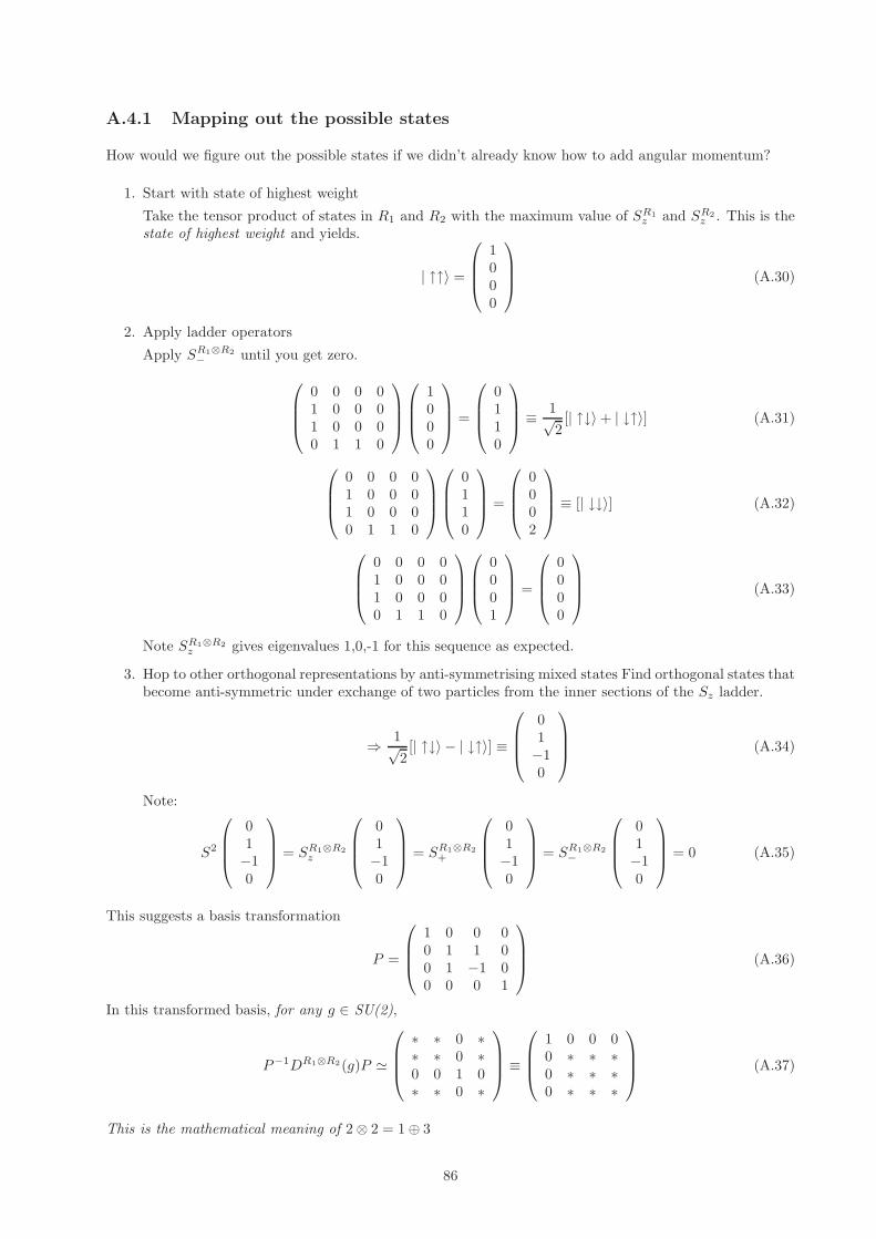
A.4.1 Mapping out the possible states

How would we figure out the possible states if we didn’t already know how to add angular momentum?

1. Start with state of highest weight

Take the tensor product of states in R1 and R2 with the maximum value of SR1z and SR2

z . This is thestate of highest weight and yields.

| ↑↑〉 =

1000

(A.30)

2. Apply ladder operators

Apply SR1⊗R2− until you get zero.

0 0 0 01 0 0 01 0 0 00 1 1 0

1000

=

0110

≡

1√2[| ↑↓〉+ | ↓↑〉] (A.31)

0 0 0 01 0 0 01 0 0 00 1 1 0

0110

=

0002

≡ [| ↓↓〉] (A.32)

0 0 0 01 0 0 01 0 0 00 1 1 0

0001

=

0000

(A.33)

Note SR1⊗R2z gives eigenvalues 1,0,-1 for this sequence as expected.

3. Hop to other orthogonal representations by anti-symmetrising mixed states Find orthogonal states thatbecome anti-symmetric under exchange of two particles from the inner sections of the Sz ladder.

⇒ 1√2[| ↑↓〉 − | ↓↑〉] ≡

01−10

(A.34)

Note:

S2

01−10

= SR1⊗R2

z

01−10

= SR1⊗R2

+

01−10

= SR1⊗R2

−

01−10

= 0 (A.35)

This suggests a basis transformation

P =

1 0 0 00 1 1 00 1 −1 00 0 0 1

(A.36)

In this transformed basis, for any g ∈ SU(2),

P−1DR1⊗R2(g)P ≃

∗ ∗ 0 ∗∗ ∗ 0 ∗0 0 1 0∗ ∗ 0 ∗

≡

1 0 0 00 ∗ ∗ ∗0 ∗ ∗ ∗0 ∗ ∗ ∗

(A.37)

This is the mathematical meaning of 2⊗ 2 = 1⊕ 3

86

Appendix B

Muon decay phase space details

We integrate the phase space for the muon decay three body final state: We consider the rest frame of themuon:

• p1 = (mµ, 0)

• p1 = p2 + p3 + p4.

• p1 · p3 = mµEνe

We have(p1 − p3)

2 = (p2 + p4)2

⇒ p2 · p4 = 12 (m2

µ −m2e)−mµEνe

Thus |M|2can be expressed purely in terms of the energy Eνe, simplifying angular integrals below. We take

the approximation me = 0, and then

dΓ = |M|2 12mµ

d3p2

(2π3)2Eνµ

d3p3

(2π3)2Eνe

d3p4

(2π3)2Ee(2π)4δ4(p1 + p2 + p3 + p4)

∫dp2 ⇒ dΓ = |M|2

16mµ

d3p3

(2π3)d3p4

(2π3)2π

EνµEνeEeδ(mµ − Eνµ

− Eνe− Ee)

where we are subject to constraints Ee = |~p4|, Eνe= |~p3|, ~pνµ

= −~p3 − ~p4, and Eνµ= |~pνµ

|.

The following sequence is the tricky bit in 3 body!

We take spherical coordinates for the p3 integral d3p3 = p23dφd cos θdp3, and θ as the angle between p3 and

p4:

dΓ = |M|216mµ

d3p4

(2π4)

∫dp3d(cos θ)

Eνe

EνµEeδ(mµ − Eνµ

− Eνe− Ee)

Observe that with u = |p2| =√|p3|2 + |p4|2 + 2|p3||p4| cos θ, then du = − p3p4 sin θdθ

p2, and so

dΓ = |M|216mµ

d3p4

(2π4)dp3

p24

∫ u=|p3+p4|u=|p3−p4| δ(mµ − Eνe

− u− Ee)du

Here energy conservation constrains which p3 values contribute a non-zero result to the integral. For thedelta function to contribute we require

|p3 − p4| ≤ mµ − |p3| − p4 ≤ |p3 + p4|

and so p3 ≥ mµ

2 − |p4|

and p3 ≤ mµ

2

87

Thus we have

dΓ = d3p4

16mµ(2π)4p24

mµ2∫

mµ2 −p4

|M|2dp3

=(

gMW

)4mµd3p4

16(2π)4p24

mµ2∫

mµ2 −p4

p3(mµ − 2p3)dp3

=(

gMW

)4mµd3p4

16(2π)4p24

[p24

mµ

2 − 23p

34

]

=(

gMW

)4mµd3p4

16(2π)4

[mµ

2 − 23p4

]

Γ =(

gMW

)4mµd3p4

8(2π)3

∫ mµ2

0 p24dp4

[mµ

2 − 23p4

]

=(

gMW

)4mµd3p4

8(2π)3

[m3

µ

96

]

=(

mµgMW

)4mµ

6144π3

88

standard model 2012

Documents