1

Standard errors of parameter estimates

in the ETAS model

Abstract

Point process models such as the Epidemic-type Aftershock Sequence (ETAS) model

have been widely used in the analysis and description of seismic catalogs and in short-

term earthquake forecasting. The standard errors of parameter estimates in the ETAS

model are significant and cannot be ignored. This paper uses simulations to explore the

accuracy of conventional standard error estimates based on the Hessian matrix of the log-

likelihood function of the ETAS model. The conventional standard error estimates based

on the Hessian are shown not to be accurate when the observed space-time window is

small. One must take caution in trusting the Hessian-based standard error estimates for

the ETAS model using typical local datasets with time windows of several years in length.

The standard errors for all parameter estimates introduced by magnitude errors in typical

earthquake catalogs are found to be smaller than those introduced by the choice of finite

time window except for the parameters and . However, neither effect is insignificant.

2

1. Introduction

The Epidemic-type Aftershock Sequence (ETAS) model is a self-

exciting point process model that descr ibes the temporal and spatial

cluster ing in earthquake catalogs. The parameters in the ETAS model

have basic physical interpretations and signif icant differences in ETAS

parameters across different regions can be used as indicators of

different focal mechanisms of earthquakes and different local stress

situations in these regions (Kagan et al. 2010). The standard errors of

parameter estimates in the ETAS model are thus very important in

determining the accuracy of particular estimates and in assessing

whether differences between estimated parameters across different

regions are signif icant.

The purpose of this paper is to investigate the accuracy of

conventional standard error estimates for parameters in the ETAS

model and to explore the impact of features such as the time per iod of

observation and size of magnitude errors on the accuracy of these

standard error estimates. In this paper, the accuracy of the

conventional standard error estimates obtained by using the Hessian

matr ix of the log-likelihood function of the ETAS model (Ogata, 1978)

is ver if ied by simulating the point processes repeatedly, estimating the

parameters corresponding to each simulation, and compar ing the

var iability in the parameter estimates in these simulations to the

conventional standard error estimates. The difference between

3

standard errors estimated based on the Hessian and those based on

simulation in finite time windows is studied. In this paper, “standard errors from (or

based on) simulation” means the standard errors are estimated by comparing estimated

parameters of simulated earthquake catalogs with the true value of the parameters;

“standard errors from (or based on) the Hessian” means the standard errors are estimated

by the Hessian matrix of the log-likelihood function of the ETAS model (Ogata, 1978).

The Expectation-Maximization (EM) type algorithm developed by Veen and Schoenberg

(2008) is a stable and reliable method to estimate the parameters of the ETAS model.

Comparing with the conventional maximum likelihood estimation for multi-parameter

models such as ETAS, this EM-type algorithm is more efficient and has advantages in

solving problems caused by dependence on choice of starting values and extreme flatness

of the likelihood function near the optimum (Schoenberg et al. 2009).

The fact that magnitudes of earthquakes are typically recorded with considerable error is

widely known (e.g. Kagan 2002, Kagan et al. 2006, Wang et al. 2009). Typically, events

in an earthquake catalog whose estimated magnitudes are below a certain minimum

magnitude threshold are removed prior to statistical analysis, but the effects of this

threshold on the resulting statistical analysis are not very well understood. Tiniti and

Mulargia (1985) showed that magnitude errors tend to result in overestimates of the total

number of events with magnitude above the minimum magnitude cutoff occurring in a

fixed space-time window and that estimates of the Gutenberg-Richter b-value are not

substantially affected by typical magnitude errors. Sornette and Werner (2005a, 2005b)

studied the relationship between the lower magnitude threshold and the

branching ratio in the ETAS model, and Schoenberg et al. (2009) showed that

the lower magnitude cutoff tends to have an approximately exponential impact on the

bias in ETAS parameter estimates, but the effect on standard error estimates has to our

knowledge not been studied previously. A focus of this paper is on the relationship of

magnitude errors on the accuracy of standard error estimates in ETAS models.

4

2. Data There are several known earthquake catalogs cover ing southern

California. Kagan et al. (2006) and Wang et al. (2009) have carefully

studied several catalogs and estimated the uncertainties of location

and magnitude in different catalogs. Based on the information they

provided, the Advanced National Seismic System (ANSS) earthquake

catalog is used in this paper. The ANSS earthquake catalog is built by

combining the Northern California Seismic Network (NCSN) catalog, the

Southern California Seismic Network (SCSN) catalog, the Berkeley

catalog, the Nevada seismic network catalog, and the National

Earthquake Information Center (NEIC) catalog. In the ANSS catalog, a

higher pr ior ity is given to the most local seismic catalog when multiple

solutions are provided (Wang et al. 2009). The ANSS catalog is

available online at http://www.ncedc.org/anss/catalog-search.html.

Earthquake completeness cannot be ignored in data selection.

Incomplete earthquake data introduces additional biases. Felzer (2008)

and Kagan et al. (2006) estimated the magnitude completeness history

in California. Based on this information, in this paper we restr ict our

5

attention to all observed earthquakes with minimum magnitude 4.0

occurred from 01/01/1979 through 01/01/2009, between

longitude and and latitude and

(approximately ). There are 876 events in this dataset.

Figure 1 shows the locations, times and magnitudes of these Southern

California earthquakes.

Note that in analyzing the standard errors of parameter estimates in

ETAS caused by magnitude errors, all earthquakes with minimum

magnitude 3.0 in the same time-space window descr ibed above are

considered before adding synthetic magnitude errors, because some

earthquakes with true magnitude smaller than 4.0 might reach

estimated magnitudes of greater than 4.0 after magnitude errors are

introduced.

3. Methods

3.1 The Epidemic-type Aftershock Sequence Model Branching point process models have been widely used in earthquake occurrence studies

(Ogata, 1988, 1992, 1998; Kagan, 1991; Kagan and Knopoff, 1987; Musmeci and Vere-

Jones, 1992; Console et al., 2003; Zhuang et al., 2002, 2004, 2005). Comparing with

traditional window-based (Utsu, 1969; Gardner and Knopoff, 1974) and link-based

(Resenberg, 1985) space-time earthquake occurrence models, branching point process

models have certain advantages, such as the tendency to avoid arbitrary choices of the

link distances and the ability to characterize intense clustering quite accurately. The

Epidemic-type Aftershock Sequence (ETAS) model introduced by Ogata (1988, 1998) is

6

currently widely used in the description of earthquake catalogs and in earthquake

forecasting. The ETAS model is a type of branching point process model that allows both

background events and triggered events to trigger the future offspring events. The model

is often called self-exciting (Hawkes, 1971), because according to the ETAS model,

earthquakes trigger aftershocks, and those aftershocks in turn produce more aftershocks,

etc.

Simple point process models are characterized quite generally by their conditional rate

(or conditional intensity), λ (Daley and Vere-Jones, 2003). represents

the expected rate of seismicity of a particular event at time t, location (x, y) and

magnitude M given information , the history of events prior to time t. For the ETAS

model, the conditional rate function can be written

(3.1)

where µ(x,y,t) is the background seismicity rate and is called the

triggering function and describes the aftershock activity induced by prior events. is

the probability density function (PDF) of the earthquake magnitudes, and is assumed not

to change in space or time according to the ETAS model (Ogata 1988, Ogata 1998). The

Gutenberg-Richter relationship (Gutenberg and Richter, 1944) describes the magnitude

distribution.

, (3.2)

where is the minimum magnitude threshold in the earthquake catalog.

Usually, one assumes that the background seismicity rate is stationary, i.e. independent of

time t. Thus (3.1) becomes

(3.3)

7

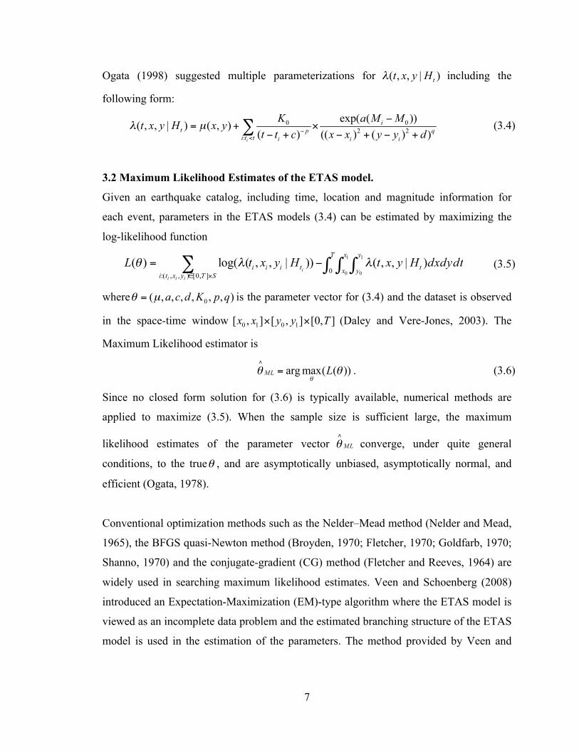
Ogata (1998) suggested multiple parameterizations for including the

following form:

(3.4)

3.2 Maximum Likelihood Estimates of the ETAS model.

Given an earthquake catalog, including time, location and magnitude information for

each event, parameters in the ETAS models (3.4) can be estimated by maximizing the

log-likelihood function

(3.5)

where is the parameter vector for (3.4) and the dataset is observed

in the space-time window (Daley and Vere-Jones, 2003). The

Maximum Likelihood estimator is

. (3.6)

Since no closed form solution for (3.6) is typically available, numerical methods are

applied to maximize (3.5). When the sample size is sufficient large, the maximum

likelihood estimates of the parameter vector converge, under quite general

conditions, to the true , and are asymptotically unbiased, asymptotically normal, and

efficient (Ogata, 1978).

Conventional optimization methods such as the Nelder–Mead method (Nelder and Mead,

1965), the BFGS quasi-Newton method (Broyden, 1970; Fletcher, 1970; Goldfarb, 1970;

Shanno, 1970) and the conjugate-gradient (CG) method (Fletcher and Reeves, 1964) are

widely used in searching maximum likelihood estimates. Veen and Schoenberg (2008)

introduced an Expectation-Maximization (EM)-type algorithm where the ETAS model is

viewed as an incomplete data problem and the estimated branching structure of the ETAS

model is used in the estimation of the parameters. The method provided by Veen and

8

Schoenberg (2008) improves the estimation of ETAS parameters and the procedure is

substantially more robust than gradient-based methods (Schoenberg, 2009). In this paper,

the EM-type algorithm in Veen and Schoenberg (2008) is used to estimate the parameters

of the ETAS model (3.4).

In order for our simulation studies to be realistic, the parameters used in these simulations

are those estimated by fitting the ETAS model (3.4) to the Southern California

earthquake dataset with minimum magnitude threshold 4.0 described in Section 2. The

resulting parameters are shown in Table 1.

Figure 2 shows the log-likelihood function for varying one parameter at a time when

applying model (3.4) to the Southern California earthquake catalog. The log-likelihood

value stays very flat as parameters , , and vary around their estimated values

while it changes substantially when parameters , and vary around their estimated

values. This is consistent with Veen (2008).

3.3 Estimates of standard errors of the ETAS parameters

The second order partial derivatives of a function describe its local curvature of the

function, and the covariance matrix of the estimated parameters can be calculated by the

inverse of the Hessian matrix or matrix of second order partial derivatives, so the

asymptotic standard errors of estimated parameters can be calculated from the Hessian

matrix. The OPTIM function in R package is used to calculate the Hessian matrix in this

paper.

Ogata (1978) showed that the standard error estimates based on the Hessian of the log-

likelihood function for stationary point processes are guaranteed to be valid

asymptotically, under general conditions, as the space-time window becomes infinite.

However, for finite space-time windows used in typical analyses of earthquake catalogs,

the standard error estimates based on the Hessian of the loglikelihood may be biased.

9

Recent improvements and advances in computation and the reliable and robust estimation

of self-exciting point process models now enable standard errors of parameters to be

estimated using simulations.

Simulation result might be instable due to the lack of the upper limit in the magnitude

distribution. If no limit is introduced, the number of earthquakes in a simulated catalog

could be very large. To avoid this problem, tapered Gutenberg-Richter distribution

(Jackson and Kagan, 1999; Kagan and Jackson 2000) is used in our simulation.

Magnitude 8 is used as the upper limit of magnitude in California.

In order to obtain estimates of the standard errors of parameters in the ETAS model, 1000

simulations of the ETAS model are obtained. For each simulation, estimates of the ETAS

parameters of the simulated earthquake process are obtained. The standard error can then

be estimated from these simulations by using the root-mean-square of the errors in the

parameter estimates for the simulations, or, in order to be more resistant to outliers, one

may instead use the median size of the errors:

Median [absolute value of (parameter estimate for simulated catalog -“true value”)],

where the “true value” is the parameter value estimated from the real earthquake catalog.

Simulation based estimates of the standard errors of the ETAS parameters might be

slightly inaccurate due to the finite number (1000) of simulations used. The bootstrap

method is used here to estimate the standard deviation of the estimated standard errors

and to assess the convergence of the simulation based estimates of standard errors.

3.4 Impact of magnitude errors

In addition to the bias introduced by the finite time-space window, biases caused by

catalog uncertainties including magnitude errors can render parameter estimates and

standard error estimates in the ETAS model inaccurate. Some researchers (e.g., Freedman,

1967; Ringdal, 1975; Rhoades, 1996) have shown that magnitude estimates

10

approximately follow the normal distribution. Here, we investigate the effect that

normally distributed magnitude errors might have on estimates of parameters and

standard error estimates. Assume that an earthquake with true magnitude is observed

as magnitude due to the normalized magnitude error with mean 0 and standard

deviation :

, (3.7)

and that the true magnitude follows the exponential (Gutenberg-Richter) density,

(3.8)

Then the distribution of m given x, and is (e.g., DeGroot, 1970; Rhoades, 1996):

(3.8)

Thus, the posterior distribution of the true magnitude is normal with mean

and standard deviation (Rhoades, 1996).

In the simulation process, the true magnitude is generated based on formula (3.8). 1000

simulations are used for each magnitude error. EM-type algorithm is used to estimate

parameters in each simulated earthquake catalog. The standard deviation of the estimated

stand error of each parameter is measured by bootstrap method.

It must be in mind that, although some earthquakes’ magnitudes are larger than 4 in the

real catalog, their true magnitude might be less than 4 after magnitude errors are

considered and vice versa.

4. Results 4.1 Simulation results on the effect of f inite time windows on standard error estimates

11

As mentioned in Section 3.3, conventional estimates of parameters and standard errors

are generally guaranteed to be asymptotically unbiased, under general regularity

conditions, as the space-time window becomes infinite. However, for typical finite space-

time windows, the bias in conventional Hessian-based standard error estimates can be

substantial. This Section summarizes the results of our investigation of this bias using

simulations of the ETAS model with parameters given in Table 1, and the space-time

window [0, 580km] x [0, 556km] and time windows of [0, T] with T between 0 and 50

years. The Gutenberg-Richter b value of 0.9912 is used in the simulations, and only

earthquakes with magnitude 4.0 or higher are used to obtain maximum likelihood

estimates for each simulation, using the EM-type algorithm.

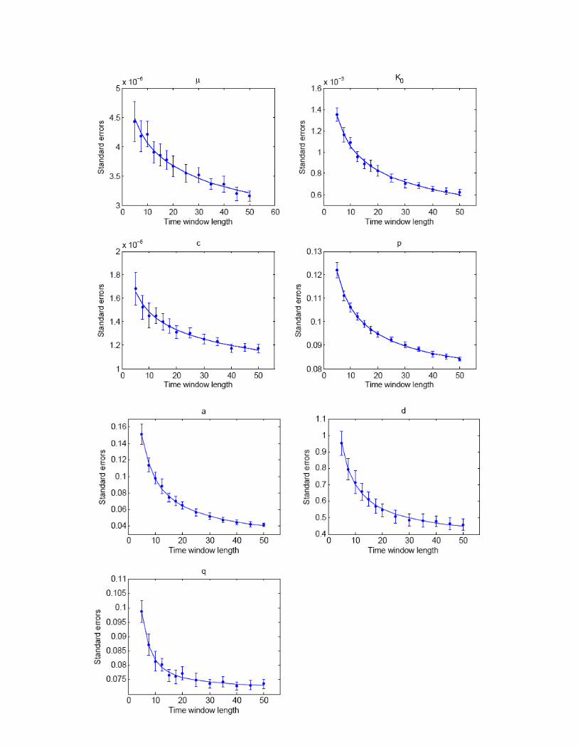
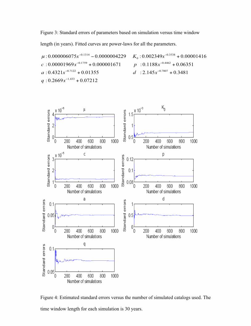
Figure 3 shows how the simulation-based standard errors of the parameter estimates

decrease as the finite time period T increases. Note that the decrease is far from linear.

For all the parameters, the simulation-based standard errors could be well fitted by power

laws. The standard deviations of the estimated standard errors in each parameter are

obtained by bootstrapping the 1000 simulation-based estimates. The 95% confidence

bounds at different time window sizes are shown in Figure 3. Note that these standard

deviations are quite small, indicating that errors in Figure 3 induced by the finite number

(1000) of simulations are quite minimal.

The stability of the estimates of the simulation-based standard errors is further verified in

Figure 4. Figure 4 shows the convergence of the estimated standard errors as the number

of simulated catalogs increases. One sees that the standard error estimates appear to have

converged after just 1000 simulated catalogs. The results shown in Figure 4 are for T =

30 years, but the results are very similar for other values of T.

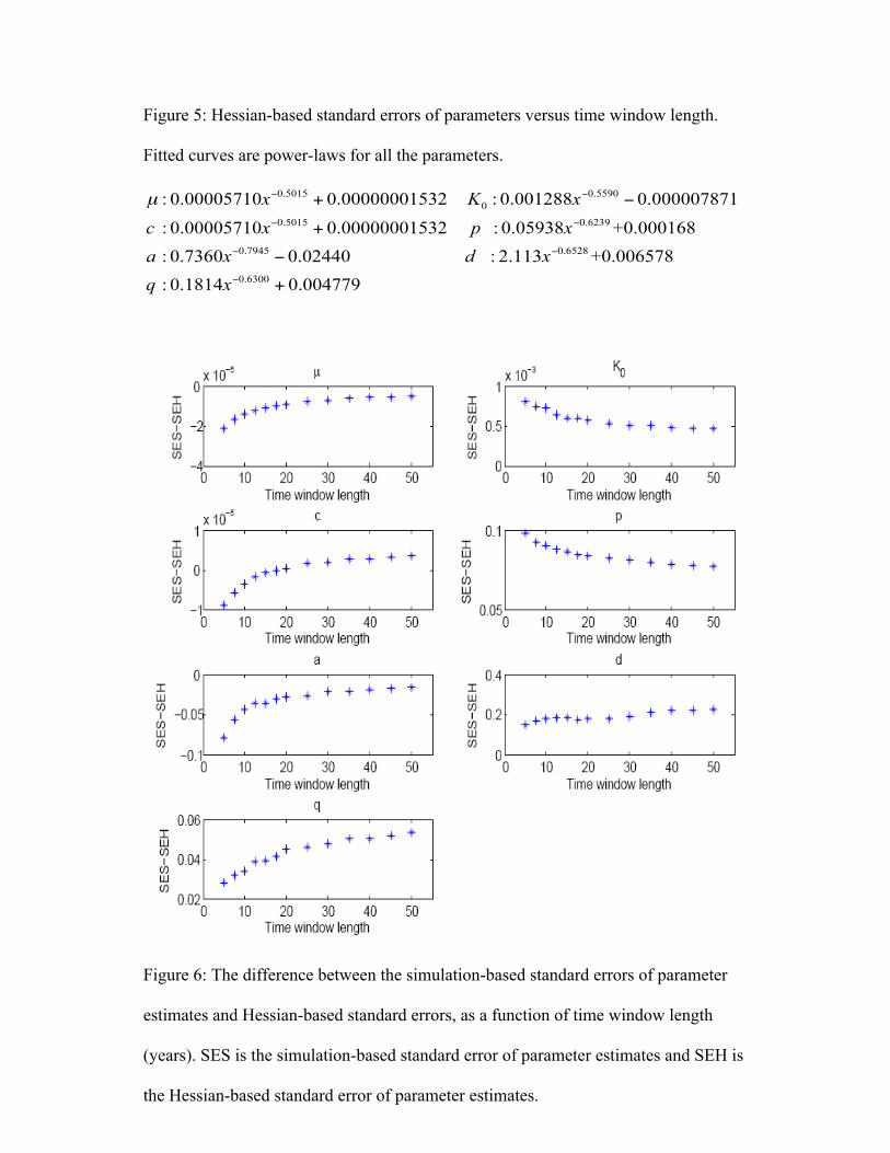
Figure 5 shows the relationship between the Hessian-based standard errors of each

parameter and the finite time period T. As with the simulation-based standard error

12

estimates in Figure 3, the Hessian-based estimates decrease nonlinearly as T increases,

and these decreases can generally be well approximated by power-law curves. The

Hessian-based standard error estimates appear to decrease a bit more smoothly than those

based on simulation as the time T increases.

Figure 6 shows the difference between the simulation-based standard errors of parameter

estimates and Hessian-based standard errors, as a function of the time window length.

Note that in such comparisons, if there is a discrepancy between the simulation-based and

Hessian-based estimate of a standard error, the simulation-based estimate should be

trusted, since it represents the actual typical size of an error in the parameter estimate,

observed in our simulations. Meanwhile the Hessian is simply based on asymptotic

formulae that do not necessarily apply to the case of a finite space-time window. For the

parameter , the simulation-based standard error is considerably smaller than that based

on the Hessian, indicating that the conventional standard error estimate of parameter

based on the Hessian is significantly biased. The standard errors based on simulation are

always larger than those based on the Hessian for parameters , , and q. For

parameter c, the standard errors based on simulation are larger when T is more than 20

years. The difference converges to 0 as T increases for parameters , , and .

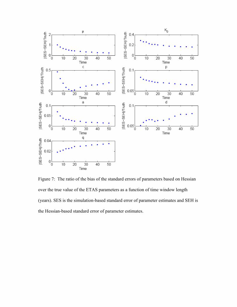
Asymptotic standard errors based on the Hessian are typically quite inaccurate and this

bias can be more than 20% of the size of the actual parameter, for small time windows of

just 5 years, for some parameters, as shown in Figure 7. Figure 7 shows the biases in the

conventional, Hessian-based standard error estimates, expressed as ratios in proportion to

the corresponding true values of the ETAS parameters. One sees from Figure 7 that the

biases in conventional standard error estimates are quite large for small time windows of

10 years or less, but become quite small for time windows of 40 years or more for

parameters , , and .

13

The estimates of different parameters in the ETAS model can be highly correlated. Figure

8 shows scatterplots of the errors (absolute value of the difference between estimate and

true parameter) of other parameters versus the simulation-based standard error of

parameter p, when T is 30 years. Table 2 shows the correlations of pairs of all parameters

when T is 30 years. Correlations among estimates of the pairs and are higher

than 0.5. This is perhaps not surprising, as the parameters simultaneously govern

the spatial distribution of aftershocks, and the pair governs the temporal decay in

aftershock activity according to the ETAS model.

4.2 The impact of magnitude errors on standard error estimates

Figure 9 shows the standard errors of the parameter estimates based on simulations as a

function of σ, the typical size of the magnitude errors. For all the parameters, the standard

errors increase approximately linearly as a function of typical magnitude error size,

though some curvature is seen in this relationship for parameters and .

Figure 10 shows how the estimated standard errors change as the number of simulations

increase, when the typical magnitude error size is 0.11. The results are very similar when

different values of σ are applied, showing that estimates of standard errors appear to be

stable and accurate when 1000 simulations are used.

Figure 11 shows the standard error of each parameter based on the Hessian, as a function

of the typical magnitude error size, σ. Unlike the standard errors estimated based on

simulations, the Hessian-based standard error estimates of all the ETAS parameters

appear to increase monotonically as σ increases and can be well approximated by

exponential curves in each case.

Comparing Figures 9 and 11, one sees that the standard errors of parameter estimates

based on the Hessian are substantially different from those based on simulation in most

cases. This is consistent with the results described in Section 4.1 and shows that the

14

asymptotic standard errors based on the Hessian are typically quite inaccurate for

standard space-time windows and magnitude error sizes.

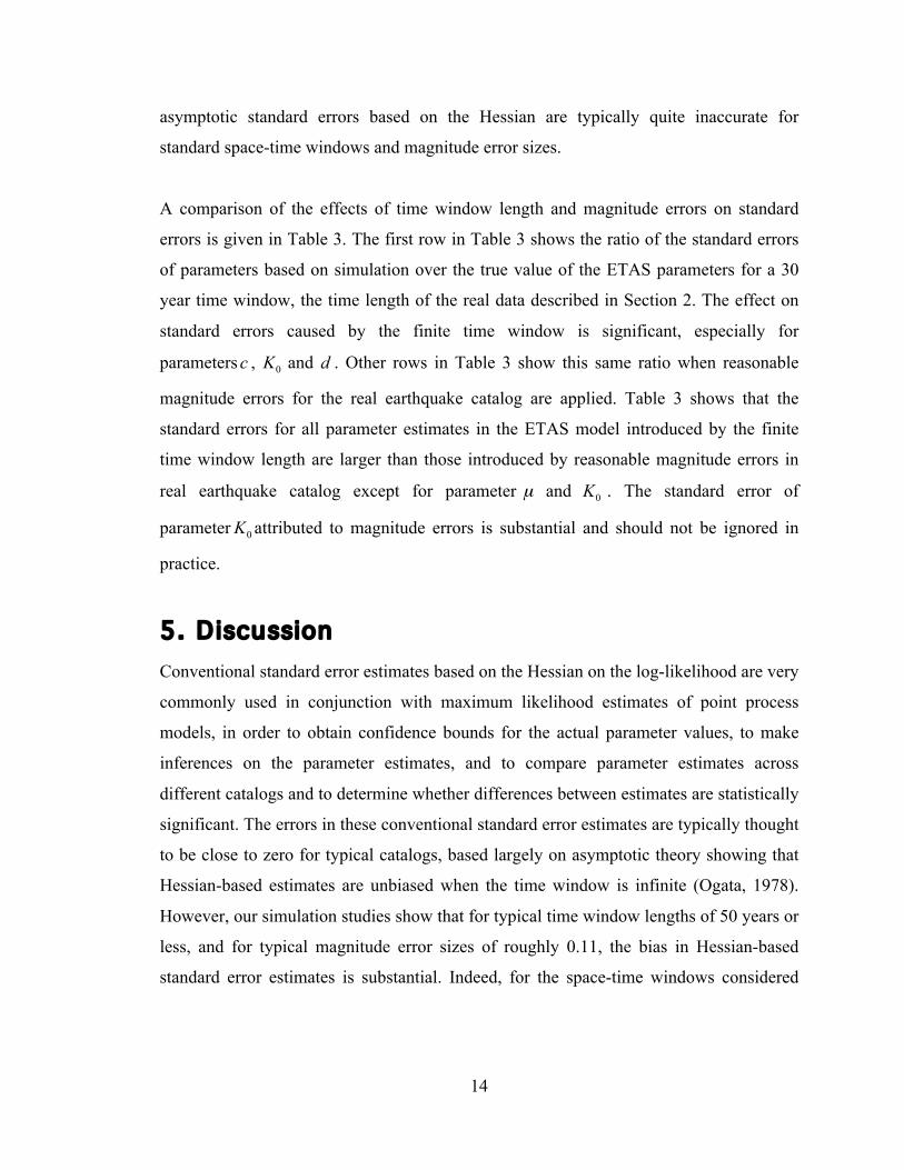
A comparison of the effects of time window length and magnitude errors on standard

errors is given in Table 3. The first row in Table 3 shows the ratio of the standard errors

of parameters based on simulation over the true value of the ETAS parameters for a 30

year time window, the time length of the real data described in Section 2. The effect on

standard errors caused by the finite time window is significant, especially for

parameters , and . Other rows in Table 3 show this same ratio when reasonable

magnitude errors for the real earthquake catalog are applied. Table 3 shows that the

standard errors for all parameter estimates in the ETAS model introduced by the finite

time window length are larger than those introduced by reasonable magnitude errors in

real earthquake catalog except for parameter and . The standard error of

parameter attributed to magnitude errors is substantial and should not be ignored in

practice.

5. D iscussion Conventional standard error estimates based on the Hessian on the log-likelihood are very

commonly used in conjunction with maximum likelihood estimates of point process

models, in order to obtain confidence bounds for the actual parameter values, to make

inferences on the parameter estimates, and to compare parameter estimates across

different catalogs and to determine whether differences between estimates are statistically

significant. The errors in these conventional standard error estimates are typically thought

to be close to zero for typical catalogs, based largely on asymptotic theory showing that

Hessian-based estimates are unbiased when the time window is infinite (Ogata, 1978).

However, our simulation studies show that for typical time window lengths of 50 years or

less, and for typical magnitude error sizes of roughly 0.11, the bias in Hessian-based

standard error estimates is substantial. Indeed, for the space-time windows considered

15

here, the biases appear to converge to 0 only for the parameters , , and . This

appears to contradict the results in Ogata (1978), but one possible explanation is that the

high correlations of some pairs of parameter estimates and the singularity of the Hessian

in some cases for the space-time ETAS model might violate the assumptions (B6) and

(C2) in Ogata (1978). Due to restrictions on computation time, it is difficult to simulate

earthquake data according to the ETAS model for thousands of years, so it is unknown

what happens when the time window approaches infinity. We leave this question for

future research. But the present study impacts the analysis of current modern earthquake

catalogs that are typically available for 100 years or less. The discrepancy might also be

cause by variables in earthquake catalogs are heavy-tailed, and the standard

statistical theory assumes them to be with a finite second moment. Zaliapin et al. (2005)

describes how heavy-tailed distributions have a very different behavior for small and

large samples. In addition, strong non-linearity in the likelihood function near

its maximum might contribute part of discrepancy. Kagan and Schoenberg (2001) shows

the problems when most of the parameters need to be positive and the likelihood value is

close to its maximum.

The influence of a catalog time limit may depend on simulation and inversion techniques.

For example, one can simulate a long sequence and then cut a shorter one from it, or

simulate a short catalog only. In this paper, we first simulated 1200 years catalog and

then cut 50 years after the earthquake rate reaches a stationary level in the simulated

samples.

Note that the background intensity in the ETAS model is assumed to be

homogenous in this paper. Whether a model with homogeneous is reasonable in

practice depends on local fault information, local stress information, etc. There are

alternative parameterizations of ETAS models, such as

(5.1)

16

Model (5.1) was introduced by Ogata (1998). The main difference between models (3.4)

and model (5.1) is that in model (3.4), the spatial region governing the triggered events is

not scaled according to the magnitude of the triggering event. Model (5.1) offered

superior fit to Japanese earthquake data in Ogata (1998), but Zhuang (2005) showed that

model (3.4) fits earthquake data in Taiwan region better than model (5.1). Further

research is needed to explore the bias and validity of conventional standard error

estimates for other ETAS parameterizations, including those with inhomogeneous

background intensity.

It is important to point out that the standard errors of parameter estimates in the ETAS

model depends on the parameters of the underlying ETAS model used in the simulation.

In other words, the standard errors of parameter estimates in the ETAS model in Figure 4

are only suitable for the dataset described in Section 2. The impact of features such as the

time period of observation and the size of magnitude errors on these standard error

estimates might be different in different regions and different time periods. However, the

same methods described in Section 3 could in principle be used to investigate standard

error estimates in other earthquake catalogs.

REFERENCES

Aki, K. (1965). Maximum likelihood estimate of b in the formula log n = a - b*m and its confidence limits. Bull. Eq. Res. Inst. 43, 237–239 Broyden, C. G. (1970), The Convergence of a Class of Double-rank Minimization Algorithms ,Journal of the Institute of Mathematics and Its Applications, 6, 76-90 Console, R., M. Murru, and A. M. Lombardi (2003), Refining earthquake clustering models, J. Geophys. Res., 108(B10), 2468, doi:10.1029/2002JB002130. Daley, D., and D. Vere-Jones (2003), An Introduction to Theory of Point Processes, Springer, New York. DeGroot, M.H.(1970), Optimal Statistical Decisions. McGraw-Hill, New York, NY, 489 pp.

17

Felzer, K. R.(2008), Calculating California seismicity rates, Appendix I in The Uniform California Earthquake Rupture Forecast, version 2 (UCERF 2): U.S. Geological Survey Open-File Report 2007-1437I and California Geological Survey Special Report 203I, 42 pp. Fletcher, R. (1970), A New Approach to Variable Metric Algorithms, Computer Journal, 13, 317-322

Fletcher, R. and Reeves, C. M. (1964) Function minimization by conjugate gradients. Computer Journal 7, 148–154.

Freedman, H.W.(1967), Estimating earthquake magnitude. Bulletin of the Seismological Society of America, 57: 747-760.

Gardner, J., and L. Knopoff (1974), Is the sequence of earthquakes in southern California, with aftershocks removed, Poissonian?, Bulletin of the Seismological Society of America, 64, 1363–1367. Goldfarb, D.(1970), A Family of Variable Metric Updates Derived by Variational Means, Mathematics of Computation, 24, 23-26 Hawkes, A.G. (1971). Point spectra of some mutually exciting point processes. Journal of the Royal Statistical Society, Series B, 33(3), 438-443. Hutton, K., E. Hauksson, J. Clinton, J. Franck, A. Guarino and N. Scheckel.(2006) Southern California seismic network update, Seismological Research Letters, 77(3), 389-395. Kagan, Y.Y. (1991), Likelihood analysis of earthquake catalogues, Geophys. J. Int., 106, 135–148. Kagan, Y.Y. (2002). Modern California earthquake catalogs and their comparison, Seismological Research Letters, 73(6), 921-929. Kagan, Y. Y., and L. Knopoff, "Statistical short-term earthquake prediction", Science, 236, 1563-1567, 1987 Kagan, Y. Y., D.D. Jackson, and Y. Rong (2006). A new catalog of southern California earthquakes, 1800-2005, Seismological Research Letters, 77(1), 30-38 Kagan, Y. Y., D. D. Jackson, and Y. F. Rong, (2007). A testable five-year forecast of moderate and large earthquakes in southern California based on smoothed seismicity, Seismological Research Letters, 78(1), 94-98.

18

Kagan, Y.Y., P. Bird, and D.D. Jackson (2010). Earthquake patterns in diverse tectonic zones of the globe, ms, Pure Appl. Geoph. (Evison issue), 167(6/7), in press. Musmeci, F., and D. Vere-Jones (1992), A space-time clustering model for historical earthquakes, Ann. Inst. Stat. Math., 44, 1–11. Nelder, J. A. and Mead, R. (1965) A simplex algorithm for function minimization, Computer Journal 7, 308–313. Ogata, Y. (1978), The asymptotic behaviour of maximum likelihood estimators for stationary point processes, Annals of the Institute of Statistical Mathematics, 30, 243–261. Ogata, Y. (1981): On Lewis’ Simulation Method for Point Processes, IEEE Transactions on Information Theory, 27, 23–31. Ogata, Y. (1988): Statistical Models for Earthquake Occurrences and Residual Analysis for Point Processes, Journal of the American Statistical Association, 83, 9–27. Ogata, Y. (1992), Detection of precursory relative quiescence before great earthquakes through a statistical model, J. Geophys. Res., 97, 19,845–19,871. Ogata, Y. (1998): Space-time point-process models for earthquake occurrences, Annals of the Institute of Statistical Mathematics, 50, 379–402. Omori, F. (1894), On after-shocks of earthquakes, J. Coll. Sci. Imp. Univ. Tokyo, 7, 111–200. Rathbun, S. L. (1993), Modelling marked spatio-temporal point patterns, Bull. Int. Stat. Inst., 55(2), 379–396. Reasenberg, P. (1985), Second-order moment of central California Seismicity, 1969–1982, J. Geophys. Res., 90(B7), 5479–5495. Rhoades, D.A.(1996), Estimation of the Gutenberg–Richter relation allowing for individual earthquake magnitude uncertainties, Tectonophysics, 258, 71–83. Ringdal, F.(1975), On the estimation of seismic detection thresholds. Bulletin of the Seismological Society of America, 65: 1631-1642.

19

Schoenberg, F. P., A. Chu and A. Veen (2009), On the relationship between lower magnitude thresholds and bias in ETAS parameter estimates, J. Geophys. Res. doi:10.1029/2009JB006387, in press. Shanno, D. F.(1970),Conditioning of Quasi-Newton Methods for Function Minimization , Mathematics of Computation , 24, 647-656 Tinti, S. and F. Mulargia (1985). Effects of magnitude uncertainties on estimating the parameters in the Gutenberg-Richter frequency-magnitude law. Bulletin of the Seismological Society of America 75, 1681–1697. Veen, A., and Schoenberg, F. (2008). Estimation of space-time branching process models in seismology using an EM-type algorithm. Journal of the American Statistical Association, 103, 614-624 Wang, Q, D.D. Jackson, and Y. Y. Kagan (2009). California earthquakes, 1800-2007: a unified catalog with moment magnitudes, uncertainties and focal mechanisms. Seismological Research Letters, 80, 446-457. Sornette, D., and Werner, M.J. (2005a). Apparent cluster ing and apparent background earthquakes biased by undetected seismicity. J. Geophys. Res. 110(B9), B09303. Sornette, D, and Werner, M.J. (2005b). Constraints on the size of the smallest tr igger ing earthquake from the ETAS Model, Baath's Law, and observed aftershock sequences. J. Geophys. Res. 110(B8), B08304. Utsu, T. (1969), Aftershock and earthquake statistics. I: Some parameters which characterize an aftershock sequence and their interrelations, J. Fac. Sci., Hokkaido Univ., Ser. VII, Geophys., 3, 129–195. Zaliapin, I. V., Y. Y. Kagan, and F. Schoenberg, 2005. Approximating the distribution of Pareto sums, Pure Appl. Geoph., 162(6-7), 1187-1228. Zhuang, J., Y. Ogata and D. Vere-Jones (2002). Stochastic declustering of space-time earthquake occurrences, Journal of the American Statistical Association, 97, 369-380

20

Zhuang, J., Y. Ogata, and D. Vere-Jones (2004), Analyzing earthquake clustering features by using stochastic reconstruction, J. Geophys. Res., 109, B05301, doi:10.1029/2003JB002879 Zhuang, J., C.-P. Chang, Y. Ogata, and Y.-I. Chen (2005), A study on the spontaneous and clustering seismicity in the Taiwan region by using point process models, J. Geophys. Res., 110, B05S18, doi:10.1029/2004JB003157.

21

Table 1 Estimated parameters of the ETAS model (3.4). Note that a homogenous

background intensity is applied.

Parameter

-0.0605

-0.0095 0.0695

-0.0097 0.244 0.580

-0.1054 0.0705 0.0257 0.0437

0.00590 -0.244 0.0402 0.0333 0.0512

0.0400 -0.407 0.018 0.0270 0.0292 0.721

Table 2: Correlations between standard errors in parameter estimates from simulation,

when the time window length is 30 years.

Space-time window

0.000020737 0.0028123 0.000018951 1.1903 1.1203 2.8240 1.5435

22

30 years

time window 5.78% 25.93% 64.39% 7.52% 4.62% 17.29% 4.60%

Magnitude

error 0.09 4.50% 27.39% 10.75% 0.26% 1.63% 5.22% 0.48%

Magnitude

error 0.11 5.07% 32.92% 12.96% 0.28% 1.71% 5.97% 0.58%

Magnitude

error 0.13 5.79% 34.37% 15.49% 0.29% 1.90% 7.54% 0.63%

Magnitude

error 0.15 6.76% 39.09% 17.39% 0.33% 1.86% 8.78% 0.67%

Table 3: The ratio of the standard errors of parameters based on simulation over the

true value of the ETAS parameters.

23

Figure 1: Location, time and magnitude relationship of the real earthquake catalog.

Top figure show the location information and bottom figure show the magnitude and

time information.

24

Figure 2: The likelihood function of the real earthquake catalog while varying one

parameter at a time.

25

26

Figure 3: Standard errors of parameters based on simulation versus time window

length (in years). Fitted curves are power-laws for all the parameters.

Figure 4: Estimated standard errors versus the number of simulated catalogs used. The

time window length for each simulation is 30 years.

27

28

Figure 5: Hessian-based standard errors of parameters versus time window length.

Fitted curves are power-laws for all the parameters.

Figure 6: The difference between the simulation-based standard errors of parameter

estimates and Hessian-based standard errors, as a function of time window length

(years). SES is the simulation-based standard error of parameter estimates and SEH is

the Hessian-based standard error of parameter estimates.

29

Figure 7: The ratio of the bias of the standard errors of parameters based on Hessian

over the true value of the ETAS parameters as a function of time window length

(years). SES is the simulation-based standard error of parameter estimates and SEH is

the Hessian-based standard error of parameter estimates.

30

Figure 8: Scatterplots of the simulation-based errors in all other parameter estimates

versus error in the parameter p, when time window length is 30 years.

31

Figure 9: Simulation-based standard errors as a function of magnitude error size.

.

32

Figure 10: Simulation-based standard error estimates versus the number of

simulations, when the typical magnitude error size is 0.11.

33

Figure 11: Hessian-based standard error estimates as a function of magnitude error size.