standard errors and confidence ... - web.ccs.miami.edu

Received 8 November 2017 Revised 23 January 2018 Accepted 2 April 2018

S P E C I A L I S S U E PA P ER

DOI 101002sim7803

Standard errors and confidence intervals for variableimportance in random forest regression classification andsurvival

Hemant Ishwaran | Min Lu

Division of Biostatistics Miller School ofMedicine University of Miami MiamiFlorida USA

CorrespondenceHemant Ishwaran Division ofBiostatistics 1120 NW 14th StreetUniversity of Miami Miami FL 33136USAEmail hemantishwarangmailcom

Funding informationNIH GrantAward Number R01GM125072

558 Copyright copy 2018 John Wiley amp Sons Ltd

Random forests are a popular nonparametric tree ensemble procedure with

broad applications to data analysis While its widespread popularity stems from

its prediction performance an equally important feature is that it provides a

fully nonparametric measure of variable importance (VIMP) A current limita-

tion of VIMP however is that no systematic method exists for estimating its

variance As a solution we propose a subsampling approach that can be used

to estimate the variance of VIMP and for constructing confidence intervals

The method is general enough that it can be applied to many useful settings

including regression classification and survival problems Using extensive

simulations we demonstrate the effectiveness of the subsampling estimator

and in particular find that the delete‐d jackknife variance estimator a close

cousin is especially effective under low subsampling rates due to its bias cor-

rection properties These 2 estimators are highly competitive when compared

with the 164 bootstrap estimator a modified bootstrap procedure designed to

deal with ties in out‐of‐sample data Most importantly subsampling is compu-

tationally fast thus making it especially attractive for big data settings

KEYWORDS

bootstrap delete‐d jackknife permutation importance prediction error subsampling VIMP

1 | INTRODUCTION

Random forests (RF)1 are a popular tree‐based learning method with broad applications to machine learning and datamining RF was originally designed for regression and classification problems but over time the methodology has beenextended to other important settings For example random survival forests (RSF)23 extends RF to right‐censoredsurvival and competing risk settings (see also Hothorn et al4 and Zhu and Kosorok5 for other tree ensemble approachesto survival analysis) Two guiding principles are at the core of RFs success One is the use of deep trees Another isinjecting randomization into the tree growing process First trees are randomly grown by using a bootstrap sampleof the data Secondly random feature selection is used when growing the tree Thus rather than splitting a node usingall variables the node is split using the best candidate from a randomly selected subset of variables The purpose of this2‐step randomization is to decorrelate trees which encourages low variance for the ensemble due to bagging6 Whencombined with the strategy of using deep trees which is a bias reduction technique this reduces generalization errorand results in superior performance for the ensemble

Statistics in Medicine 201938558ndash582wileyonlinelibrarycomjournalsim

ISHWARAN AND LU 559

While RFs popularity stems from its prediction performance an equally important feature is that it provides a fullynonparametric measure of variable importance (VIMP)127-9 Variable importance allows users to identify whichvariables play a key role in prediction thus providing insight into the underlying mechanism for what otherwise mightbe considered a black box We note that the concept of VIMP is not specific to RF and has a long history One of theearliest examples was CART10 which calculated VIMP by summing the reduction in node impurity due to a variableover all tree nodes Another approach calculated importance using surrogate splitting (see chapter 53 of Breimanet al10)

Early prototypes of RF software developed by Leo Breiman and his student Adele Cutler provided for variousoptions for calculating VIMP11 One procedure used for classification forests was to estimate VIMP using the forest aver-aged decrease in Gini impurity (somewhat akin to the node impurity approaches of CART) However while Gini impor-tance12 saw widespread initial use with RF over time it has become less popular8 By far the most frequently usedmeasure of importance was another measure provided by the Breiman‐Cutler software called permutation importance(sometimes also referred to as Breiman‐Cutler importance) Unlike Gini importance that estimates importance using in‐sample impurity permutation importance adopts a prediction‐based approach by using prediction error attributable tothe variable A clever feature is that rather than using cross‐validation which is computationally expensive for forestspermutation importance estimates prediction error by making use of out‐of‐bootstrap cases Recall that each tree is cal-culated from a bootstrap sample of the original data The approximately 1minus632=368 left from the bootstrap representsout‐of‐sample data which can be used for estimating prediction performance These data are called out‐of‐bag (OOB)and prediction error obtained from it is called OOB error13 Permutation importance permutes a variables OOB dataand compares the resulting OOB prediction error to the original OOB prediction errormdashthe motivation being that alarge positive value indicates a variable with predictive importance

Permutation (Breiman‐Cutler) Importance

In the OOB cases for a tree randomly permute all values of the jth variable Put these new covariate valuesdown the tree and compute a new internal error rate The amount by which this new error exceeds theoriginal OOB error is defined as the importance of the jth variable for the tree Averaging over the forestyields VIMP

mdash Measure 1 (Manual On Setting Up Using And Understanding Random Forests V31)

We focus on Breiman‐Cutler permutation importance in this manuscript (for simplicity hereafter simply referred toas VIMP) One of the tremendous advantages of VIMP is that it removes the arbitrariness of having to select a cutoffvalue when determining the effectiveness of a variable Regardless of the problem a VIMP of zero always representsan appropriate cutoff as it reflects the point at which a variable no longer contributes predictive power to the modelHowever in practice one may observe values close to zero and the meaning of what constitutes being zero becomesunclear One way to resolve this is to calculate the variance of VIMP but this is challenging due to the complex natureof RF Unfortunately while the empirical properties of VIMP are well documented14-16 much less is known aboutVIMPs theoretical properties outside of a few studies717

Given the difficulties of theoretical analysis an alternative approach is to approximate the distribution of VIMPthrough some form of resampling This has been the favored approach used for RF regression for assessing variabilityof RF predicted values Methods that have been used include bootstrapping18 for estimating the variance and the infin-itesimal jackknife19 and infinite order U‐statistics20 for confidence intervals These methods however only apply to RFpredicted values and not to VIMP which involves prediction error This greatly complicates matters and requires a moregeneral approach

For this reason we base our approach on subsampling21 a general methodology for approximating the distributionof a complex statistic Section 3 provides a description of our subsampling procedure for estimating the variance Nota-tional framework and a formal definition of VIMP are provided in Section 2 Section 3 begins by introducing a bootstrapsolution to be used as a comparison procedure Interestingly we find the bootstrap cannot be applied directly due to tiesthat occur in the OOB data This is precisely due to the fact that VIMP is prediction error based We propose a solutionto this problem called the 164 bootstrap estimator The subsampling variance estimator and the delete‐d jackknife var-iance estimator22 a close cousin are described later in Section 3 Sections 4 5 and 6 consider regression classificationand survival settings and extensively evaluate performance of the 2 subsampling methods and the 164 bootstrap

560 ISHWARAN AND LU

estimator We also show how to construct confidence intervals for VIMP using the estimated variance The results arevery promising for the subsampling methods Section 7 summarizes our findings and provides practical guidelines foruse of the methodology Some theoretical results for VIMP are provided in the appendix

2 | NOTATIONAL FRAMEWORK AND DEFINITION OF VIMP

21 | Notation

We assume YisinY is the response and XisinX is the p‐dimensional feature where Y can be continuous binary categoricalor survival and X can be continuous or discrete We assume the underlying problem involves a nonparametric regres-sion framework where the goal is to estimate a functional h(x) of the response given X=x Estimation is based on thelearning data L frac14 fethX1Y 1THORNhellip ethXnYnTHORNg where (XiYi) are independently distributed with the same distribution P as(XY)

Examples of h(x) are the following1 The conditional mean hethxTHORN frac14 Efrac12Y jX frac14 x in regression2 The conditional class probabilities h(x)=(p1(x)hellippK(x)) in a K‐multiclass problem where pkethxTHORN frac14 PfY frac14 kjX frac14 xg3 The survival function hethxTHORN frac14 PfTogttjX frac14 xg in survival analysis Here Y=(T δ) represents the bivariate response

composed of the observed survival time T frac14 minethToCoTHORN and censoring indicator δ=1ToleCo where (ToCo) arethe unobserved event and censoring times

22 | Random forest predictor

As in Breiman1 we define an RF as a collection of randomized tree predictors fhethmiddotΘmLTHORNm frac14 1hellipMg Here hethxΘmLTHORN denotes the mth random tree predictor of h(x) and Θm are independent identically distributed randomquantities encoding the randomization needed for constructing a tree Note that Θm is selected prior to growing the treeand is independent of the learning data L

The tree predictors are combined to form the finite forest estimator of h(x)

hethxΘ1hellipΘM LTHORN frac14 1M

sumM

mfrac141hethxΘmLTHORN (1)

The infinite forest estimator is obtained by taking the limit as Mrarrinfin and equals

hethxLTHORN frac14 EΘfrac12hethxΘLTHORN (2)

23 | Loss function

Calculating VIMP assumes some well‐defined notion of prediction error Therefore we assume there is an appropriately

prechosen loss function ℓethY ĥTHORNge0 used to measure performance of a predictor ĥ in predicting h Examples include thefollowing1 Squared error loss ℓethY ĥTHORN frac14 ethYminusĥTHORN2 in regression problems2 For classification problems widely used measures of performance are the misclassification error or the Brier score

For the latter ℓethY ĥTHORN frac14 eth1=KTHORNsumKkfrac141eth1fY frac14 kgminuspkTHORN2 where pk is the estimator for the conditional probability pk

3 For survival the weighted Brier score2324 can be used Section 6 provides further details

The choice of ℓ can be very general and we do not impose any specific conditions on how it must be selected Asdescribed later in Section 3 the conditions needed for our methodology to hold require only the existence of a limitingdistribution for VIMP Although such a limit may be satisfied by imposing specific conditions on ℓ such as requiring thetrue function h to yield the minimum value of Efrac12ℓethY hTHORN we do not impose such assumptions so as to retain as generalan approach as possible

ISHWARAN AND LU 561

24 | Tree VIMP

LetLlowastethΘmTHORN be the mth bootstrap sample and letLlowastlowastethΘmTHORN frac14 L∖LlowastethΘmTHORN be the corresponding OOB data Write X=(X(1)hellipX(p)) where X(j) denotes the jth feature coordinate The permuted value of the jth coordinate of X is denoted by ~X eth jTHORNSubstituting this into the jth coordinate of X yields ~Xeth jTHORN

~Xeth jTHORN frac14 ethX eth1THORNhellipX eth jminus1THORN ~Xeth jTHORNXeth jthorn1THORNhellipX ethpTHORNTHORN

Variable importance is calculated by taking the difference in prediction error under the original X to prediction error

under the perturbed ~Xeth jTHORN over OOB data More formally let IethXeth jTHORNΘmLTHORN denote the VIMP for X(j) for the mth treeIt follows that

IethXeth jTHORNΘmLTHORN frac14sumiisinLlowastlowastethΘmTHORNℓethYi heth~Xeth jTHORN

i ΘmLTHORNTHORNsumiisinLlowastlowastethΘmTHORN1

minussumiisinLlowastlowastethΘmTHORNℓethYi hethXiΘmLTHORNTHORN

sumiisinLlowastlowastethΘmTHORN1 (3)

Note that in the first sum we implicitly assume Θm embeds the additional randomization for permuting OOB data to

define ~Xeth jTHORNi Because this additional randomization only requires knowledge of OOB membership and therefore can

be parameterized in terms of Θ we assume without loss of generality that Θ encodes both the randomization for grow-ing a tree and for permuting OOB data

Expression (3) can be written more compactly by noting that the denominator in each sum equals the OOB samplesize Let N(Θm) be this value Then

IethXeth jTHORNΘmLTHORN frac14 1NethΘmTHORN sum

iisinLlowastlowastethΘmTHORNfrac12ℓethYi heth~Xeth jTHORN

i ΘmLTHORNTHORNminusℓethYi hethXiΘmLTHORNTHORN

25 | Variable importance

Averaging tree VIMP over the forest yields VIMP

IethX eth jTHORNΘ1hellipΘM LTHORN frac14 1M

sumM

mfrac141IethXeth jTHORNΘmLTHORN (4)

An infinite forest estimator for VIMP can be defined analogously by taking the limit as Mrarrinfin

IethX eth jTHORNLTHORN frac14 EΘfrac12IethX eth jTHORNΘLTHORN (5)

It is worth noting that (4) and (5) do not explicitly make use of the forest predictors (1) or (2) This is a unique feature ofpermutation VIMP because it is a tree‐based estimator of importance

3 | SAMPLING APPROACHES FOR ESTIMATING VIMP VARIANCE

31 | The 164 bootstrap estimator

The bootstrap is a popular method that can be used for estimating the variance of an estimator So why not use the boot-strap to estimate the standard error for VIMP One problem is that running a bootstrap on a forest is computationallyexpensive Another more serious problem however is that a direct application of the bootstrap will not work for VIMPThis is because RF trees already use bootstrap data and applying the bootstrap creates double‐bootstrap data that affectsthe coherence of being OOB

To explain what goes wrong let us simplify our previous notation by writing Ieth jTHORNnM for the finite forest estimator (4)

Let Pn denote the empirical measure for L The bootstrap estimator of VarethIeth jTHORNnMTHORN is

562 ISHWARAN AND LU

VarlowastethIeth jTHORNnMTHORN frac14 VarPnethIlowasteth jTHORNnMTHORN (6)

To calculate (6) we must draw a sample from Pn Call this bootstrap sample Llowast Because Llowast represents the learningdata we must draw a bootstrap sample from Llowast to construct a RF tree Let LlowastethΘlowastTHORN denote this bootstrap sample whereΘlowast represents the tree growing instructions This is a double‐bootstrap draw The problem is that if a specific case in Llowast

is duplicated lgt1 times there is no guarantee that all l cases appear in the bootstrap draw LlowastethΘlowastTHORN These remainingduplicated values are assigned to the OOB data but these values are not truly OOB which compromises the coherenceof the OOB data

Double‐bootstrap data lower the probability of being truly OOB to a value much smaller than 368 which is thevalue expected for a true OOB sample We can work out exactly how much smaller this probability is Let ni be the num-ber of occurrences of case i in Llowast Then

Prfi is truly OOB inLlowastethΘlowastTHORNg frac14 sumn

lfrac141Prfi is truly OOB inLlowastethΘlowastTHORNjni frac14 lgPr fni frac14 lg (7)

We have

ethn1hellipnnTHORNsimMultinomialethn eth1=nhellip 1=nTHORNTHORNnisimBinomialethn 1=nTHORN≍Poissoneth1THORN

Hence (7) can be seen to equal

sumn

lfrac141

nminusln

n

Prfni frac14 lg≍sumn

lfrac141

nminusln

n eminus11l

l

frac14 eminus1sum

n

lfrac1411minus

ln

n1l≍eminus1sum

n

lfrac141

eminusl

l≍1635

Therefore double‐bootstrap data have an OOB size of 164nThe above discussion points to a simple solution to the problem which we call the 164 bootstrap estimator The 164

estimator is a bootstrap variance estimator but is careful to use only truly OOB data Let Llowast frac14 fZ1 frac14 ethXi1 Yi1THORNhellipZn frac14 ethXin YinTHORNg denote the bootstrap sample used for learning and letLlowastethΘlowastTHORN frac14 fZiiisinΘlowastg be the bootstrap sample usedto grow the tree The OOB data for the double‐bootstrap data are defined as fethXil YilTHORNnotinLlowastethΘlowastTHORNg However there isanother subtle issue at play regarding duplicates in the OOB data Even though fethXil YilTHORNnotinLlowastethΘlowastTHORNg are data points fromLlowast truly excluded from the double‐bootstrap sample and therefore technically meet the criteria of being OOB there is noguarantee they are all unique This is because these values originated fromLlowast a bootstrap draw and therefore could verywell be duplicated To ensure this does not happen we further process the OOB data to retain only the unique values

The steps for implementing the 164 estimator can be summarized as follows

164 bootstrap estimator for VarethIeth jTHORNnMTHORN

1 Draw a bootstrap sample Llowast frac14 fZ1 frac14 ethXi1 Yi1THORNhellipZn frac14 ethXin YinTHORNg2 Let LlowastethΘlowastTHORN frac14 fZiiisinΘlowastg be a bootstrap draw from Llowast Use LlowastethΘlowastTHORN to grow a tree predictor3 Define OOB data to be the unique values in fethXil YilTHORNnotinLlowastethΘlowastTHORNg4 Calculate the tree VIMP IethXeth jTHORNΘlowastLlowastTHORN using OOB data of step 35 Repeat steps 2 to 4 independently M times Average the VIMP values to obtain θlowasteth jTHORNn 6 Repeat the entire procedure Kgt1 times obtaining θlowasteth jTHORNn1 hellip θ

lowasteth jTHORNnK Estimate VarethIeth jTHORNnMTHORN by the bootstrap sample

variance eth1=KTHORNsumKkfrac141ethθlowasteth jTHORNnk minus

1KsumK

kprimefrac141θlowasteth jTHORNnkprime

THORN2

32 | Subsampling and the delete‐d jackknife

A problem with the 164 bootstrap estimator is that its OOB data set is smaller than a typical OOB estimator Truly OOBdata from a double bootstrap can be less than half the size of OOB data used in a standard VIMP calculation (164

ISHWARAN AND LU 563

versus 368) Thus in a forest of 1000 trees the 164 estimator uses about 164 trees on average to calculate VIMP for acase compared with 368 trees used in a standard calculation This can reduce efficiency of the 164 estimator Anotherproblem is computational expense The 164 estimator requires repeatedly fitting RF to bootstrap data which becomesexpensive as n increases

To avoid these problems we propose a more efficient procedure based on subsampling theory21 The idea rests oncalculating VIMP over small iid subsets of the data Because sampling is without replacement this avoid ties in theOOB data that creates problems for the bootstrap Also because each calculation is fast the procedure is computation-ally efficient especially in big n settings

321 | Subsampling theory

We begin by first reviewing some basic theory of subsampling Let X1hellipXn be iid random values with common distri-

bution P Let θn frac14 θethX1hellipXnTHORN be some estimator for θ(P) an unknown real‐valued parameter we wish to estimateThe bootstrap estimator for the variance of θn is based on the following simple idea Let Pn frac14 eth1=nTHORNsumn

ifrac141δXi be theempirical measure for the data Let Xlowast

1 hellipXlowastn be a bootstrap sample obtained by independently sampling n points from

Pn Because Pn converges to P we should expect the moments of the bootstrap estimator θlowastn frac14 θethXlowast1 hellipX

lowastnTHORN to closely

approximate those of θ In particular we should expect the bootstrap variance VarPnethθlowastnTHORN to closely approximate

VarethθnTHORN This is the rationale for the variance estimator (6) described earlierSubsampling21 employs the same strategy as the bootstrap but is based on sampling without replacement For b=b(n)

such that bnrarr0 let Sb be the entire collection of subsets of 1hellipn of size b For each s=i1hellipibisinSb let θnbs frac14θethXi1 hellipXibTHORN be the estimator evaluated using s The goal is to estimate the sampling distribution of n1=2ethθnminusθethPTHORNTHORN Itturns out that subsampling provides a consistent estimate of this distribution under fairly mild conditions LetQn denotethe distribution of n1=2ethθnminusθethPTHORNTHORN Assume Qn converges weakly to a proper limiting distribution Q

Qn dQ (8)

Then it follows21 that the distribution function for the statistic n1=2ethθnminusθethPTHORNTHORN can be approximated by the subsamplingestimator

ŨnbethxTHORN frac14 1Cb

sumsisinSb

1fb1=2ethθnbsminusθnTHORNlexg (9)

where Cb frac14 nb

is the cardinality of Sb More formally assuming (8) and bnrarr0 for brarrinfin then ŨnbethxTHORNp FethxTHORN frac14

Qfrac12minusinfin x for each x that is a continuity point of the limiting cumulative distribution function F The key to this argumentis to recognize that because of (8) and bnrarr0 Ũnb closely approximates

UnbethxTHORN frac14 1Cb

sumsisinSb

1fb1=2ethθnbsminusθethPTHORNTHORNlexg

which is a U‐statistic25 of order b (see Politis and Romano21 for details)

The ability to approximate the distribution of θn suggests similar to the bootstrap that we can approximatemoments of θn with those from the subsampled estimator in particular we should be able to approximate the varianceUnlike the bootstrap however subsampled statistics are calculated using a sample size b and not n Therefore to esti-mate the variance of θn we must apply a scaling factor to correct for sample size The subsampled estimator for the var-iance is (see Radulović26 and section 331 from Politis and Romano21)

υb frac14 b=nCb

sumsisinSb

θnbsminus1Cb

sumsprimeisinSb

θnbsprime

2

(10)

The estimator (10) is closely related to the delete‐d jackknife22 The delete‐d estimator works on subsets of size r=nminusdand is defined as follows

564 ISHWARAN AND LU

υJethdTHORN frac14 r=dCr

sumsisinSr

ethθnrsminusθnTHORN2

With a little bit or rearrangement this can be rewritten as follows


sumsisinSr

θnrsminus1Cr

sumsprimeisinSr

θnrsprime

2

thorn rd

1Cr

sumsisinSr

θnrsminusθn

2

Setting d=nminusb we obtain

υJethdTHORN frac14 b=ethnminusbTHORNCb

sumsisinSb

θnbsminus1Cb

sumsprimeisinSb

θnbsprime

2

thorn bnminusb

1Cb

sumsisinSb

θnbsminusθn

2

|fflfflfflfflfflfflfflfflfflfflfflfflfflfflfflfflfflzfflfflfflfflfflfflfflfflfflfflfflfflfflfflfflfflfflbias

(11)

The first term closely approximates (10) since bnrarr0 while the second term is a bias estimate of the subsampled estima-tor Thus the delete‐d estimator (11) can be seen to be a bias corrected version of (10) Furthermore this correction isalways upwards because the bias term is squared and always positive

322 | Subsampling and delete‐d jackknife algorithms

We can now describe our subsampling estimator for the variance of VIMP In the following we assume b is some inte-ger much smaller than n such that bnrarr0

b‐subsampling estimator for VarethIeth jTHORNnMTHORN1 Draw a subsampling set sisinSb Let Ls be L restricted to s2 Calculate Ieth jTHORNnMethLsTHORN the finite forest estimator for VIMP using Ls Let θ

eth jTHORNnbs denote this value

3 Repeat Kgt1 times obtaining θeth jTHORNnbs1hellip θeth jTHORNnbsK

Estimate VarethIeth jTHORNnMTHORN by frac12b=ethnKTHORNsumKkfrac141ethθeth jTHORNnbsk

minus1KsumK

kprimefrac141θeth jTHORNnbskprime

THORN2

The delete‐d jackknife estimator is obtained by a slight modification to the above algorithm

delete‐d jackknife estimator ethd frac14 nminusbTHORN for VarethIeth jTHORNnMTHORN1 Using the entire learning set L calculate the forest VIMP estimator Ieth jTHORNnMethLTHORN Let θeth jTHORNn denote this value2 Run the b‐subsampling estimator but replace the estimator in step 3 with fb=frac12ethnminusbTHORNKgsumK

kfrac141ethθeth jTHORNnbskminusθeth jTHORNn THORN2

4 | RANDOM FOREST REGRESSION RF ‐R

41 | Simulations

In the following sections (Sections 4 5 and 6) we evaluate the performance of the 164 bootstrap estimator the b‐sub-sampling estimator and the delete‐d jackknife variance estimator We begin by looking at the regression setting Weused the following simulations to assess performance

1 y frac14 10 sinethπx1x2THORN thorn 20ethx3minus05THORN2 thorn 10x4 thorn 5x5 thorn ε xjsimU(0 1) εsimN(0 1)2 y frac14 ethx21 thorn frac12x2x3minusethx2x4THORNminus12THORN1=2 thorn ε x1simU(0 100) x2simU(40π 560π) x3simU(0 1) x4simU(1 11) εsimN(0 1252)3 y frac14 tanminus1ethfrac12x2x3minusethx2x4THORNminus1=x1THORN thorn ε x1simU(0 100) x2simU(40π 560π) x3simU(0 1) x4simU(1 11) εsimN(0 12)4 y frac14 x1x2 thorn x23minusx4x7 thorn x8x10minusx26 thorn ε xjsimU(minus1 1) εsimN(0 12)5 y frac14 1fx1gt0g thorn x32 thorn 1fx4 thorn x6minusx8minusx9gt1thorn x10g thorn expethminusx22THORN thorn ε xjsimU(minus1 1) εsimN(0 12)

ISHWARAN AND LU 565

6 y frac14 x21 thorn 3x22x3expethminusjx4jTHORN thorn x6minusx8 thorn ε xjsimU(minus1 1) εsimN(0 12)7 y frac14 1fx1 thorn x34 thorn x9 thorn sinethx2x8THORN thorn εgt038g xjsimU(minus1 1) εsimN(0 12)8 y frac14 logethx1 thorn x2x3THORNminusexpethx4xminus15 minusx6THORN thorn ε xjsimU(05 1) εsimN(0 12)9 y frac14 x1x22jx3j1=2 thorn lfloorx4minusx5x6rfloorthorn ε xjsimU(minus1 1) εsimN(0 12)10 y frac14 x3ethx1 thorn 1THORNjx2jminusethx25frac12jx4j thorn jx5j thorn jx6jminus1THORN1=2 thorn ε xjsimU(minus1 1) εsimN(0 12)11 y frac14 cosethx1minusx2THORN thorn sinminus1ethx1x3THORNminustanminus1ethx2minusx23THORN thorn ε xjsimU(minus1 1) εsimN(0 12)12 y= ε εsimN(0 1)

In all 12 simulations the dimension of the feature space was set to p=20 This was done by adding variables unre-lated to y to the design matrix We call these noise variables In simulations 1 to 3 noise variables were U(0 1) for sim-ulations 4 to 11 noise variables were U(minus1 1) and for simulation 12 noise variables were N(0 1) All features (strongand noisy) were simulated independently Simulations 1 to 3 are the well‐known Friedman 1 2 3 simulations627 Sim-ulations 4 to 11 were inspired from COBRA28 Simulation 12 is a pure noise model

The sample size was set at n=250 Subsampling was set at a rate of b=n12 which in this case is b=158 We cansee that practically speaking this is a very small sample size and allows subsampled VIMP to be rapidly computedThe value of d for the delete‐d jackknife was always set to d=nminusb The number of bootstraps was set to 100 and thenumber of subsamples was set to 100 Note that this is not a large number of bootstraps or subsampled replicatesHowever they represent values practitioners are likely to use in practice especially for big data due tocomputational costs

All RF calculations were implemented using the randomForestSRC R‐package29 The package runs in OpenMPparallel processing mode which allows for parallel processing on user desktops as well as large scale computing clus-ters The package now includes a dedicated function ldquosubsamplerdquo which implements the 3 methods studied here Thesubsample function was used for all calculations All RF calculations used 250 trees Tree nodesize was set to 5 and p3 random feature selection used (these are default settings for regression) Each simulation was repeated independently250 times Random forest parameters were kept fixed over simulations All calculations related to prediction error and

VIMP were based on squared error loss ℓethY ĥTHORN frac14 ethYminusĥTHORN2

42 | Estimating the true finite standard error and true finite VIMP

Each procedure provides an estimate of the VarethIeth jTHORNnMTHORN We took the square root of this to obtain an estimate for the stan-

dard error of VIMP ethVarethIeth jTHORNnMTHORNTHORN1=2 To assess performance in estimating the standard error we used the following strat-egy to approximate the unknown parameter VarethIeth jTHORNnMTHORN For each simulation model we drew 1000 independent copies ofthe data and for each of these copies we calculated the finite forest VIMP Ieth jTHORNnM The same sample size of n=250 wasused and all forest tuning parameters were kept the same as outlined above We used the variance of these 1000 valuesto estimate VarethIeth jTHORNnMTHORN We refer to the square root of this value as the true finite standard error Additionally we aver-aged the 1000 values to estimate Efrac12Ieth jTHORNnM frac14 Efrac12IethXeth jTHORNLTHORN We call this the true finite VIMP

43 | Results

Performance of methods was assessed by bias and standardized mean‐squared error (SMSE) The bias for a method wasobtained by averaging its estimated standard error over the 250 replications and taking the difference between this andthe true finite standard error Mean‐squared error was estimated by averaging the squared difference between amethods estimated value for the standard error and the true finite standard error Standardized mean‐squared errorwas defined by dividing MSE by the true finite standard error In evaluating these performance values we realized itwas important to take into account signal strength of a variable In our simulations there are noisy variables with nosignal There are also variables with strong and moderately strong signal Therefore to better understand performancedifferences results were stratified by size of a variables true finite VIMP In total there were 240 variables to be dealtwith (12 simulations each with p=20 variables) These 240 variables were stratified into 6 groups based on 10th 25th50th 75th and 90th percentiles of true finite VIMP (standardized by the Y variance to make VIMP comparable acrosssimulations) Bias and SMSE for the 6 groups are displayed in Figure 1

All methods exhibit low bias for small VIMP As VIMP increases corresponding to stronger variables bias for thesubsampling estimator increases Its bias is negative showing that it underestimates variance The delete‐d estimator

FIGURE 1 Bias and standardized mean‐squared error (SMSE) performance for estimating VIMP standard error from random forestndash

regression simulations In total there are 240 variables (12 simulations p=20 variables in each simulation) These 240 variables have been

stratified into 6 groups based on 10th 25th 50th 75th and 90th percentiles of true finite VIMP Extreme right boxplots labeled ldquoALLrdquo display

performance for all 240 variables simultaneously [Colour figure can be viewed at wileyonlinelibrarycom]

566 ISHWARAN AND LU

does much better This is due to the bias correction factor discussed earlier (see (11)) which kicks in when signalincreases The pattern seen for bias is reflected in the results for SMSE the delete‐d is similar to the subsampling esti-mator except for large VIMP where it does better Overall the 164 estimator is the best of all 3 methods On the otherhand it is hundreds of times slower

This shows that the delete‐d estimator should be used when bias is an issue However bias of the subsampling esti-mator can be improved by increasing the subsampling rate Figure 2 reports the results from the same set of simulationsbut using an increased sampling rate b=n34 (b=628) Both estimators improve overall but note the improvement inbias and SMSE for the subsampling estimator relative to the delete‐d estimator Also notice that both estimators nowoutperform the 164 bootstrap

44 | Confidence intervals for VIMP

The subsampling distribution (9) discussed in Section 3 can also be used to calculate nonparametric confidence inter-vals21 The general idea for constructing a confidence interval for a target parameter θ(P) is as follows Define the

1minusα quantile for the subsampling distribution as cnbeth1minusαTHORN frac14 inffx~UnbethxTHORNge1minusαg Similarly define the 1minusα quantilefor the limiting distribution Q of n1=2ethθnminusθethPTHORNTHORN as ceth1minusαTHORN frac14 infftFethxTHORN frac14 Qfrac12minusinfin xge1minusαg Then assuming (8) andbnrarr0 the interval

FIGURE 2 Results from random forestndashregression simulations but with increased subsampling rate b=n34 Notice the improvement in

bias and standardized mean‐squared error (SMSE) for the subsampling estimator [Colour figure can be viewed at wileyonlinelibrarycom]

ISHWARAN AND LU 567

frac12θnminusnminus1=2cnbeth1minusαTHORNinfinTHORN (12)

contains θ(P) with asymptotic probability 1minusα if c(1minusα) is a continuity point of FWhile (12) can be used to calculate a nonparametric confidence interval for VIMP we have found that a more stable

solution can be obtained if we are willing to strengthen our asssumptions to include asympotic normality Let θeth jTHORNn frac14 Ieth jTHORNnM

denote the finite forest estimator for VIMP We call the limit of θeth jTHORNn as n Mrarrinfin the true VIMP and denote thisvalue by θeth jTHORN0

θeth jTHORN0 frac14 limnMrarrinfin

θeth jTHORNn frac14 limnMrarrinfin

Ieth jTHORNnM

Let υeth jTHORNn be an estimator for VarethIeth jTHORNnMTHORN Assuming asymptotic normality

θeth jTHORNn minusθeth jTHORN0ffiffiffiffiffiffiffiυeth jTHORNn

q dNeth0 1THORN (13)

an asymptotic 100(1minusα)confidence region for θeth jTHORN0 the true VIMP can be defined as

θeth jTHORNn plusmnzα=2

ffiffiffiffiffiffiffiυeth jTHORNn

q

where zα2 is the 1minusα2‐quantile from a standard normal PrN(0 1)le zα2=1minusα2

45 | Justification of normality

To provide justification for assumption (13) we reran our previous simulations 1000 times independently For eachMonte Carlo replication and each simulation model we calculated the finite forest VIMP for a variable and centeredit by its mean value from the 1000 simulations and divided this centered value by the standard deviation of the 1000VIMP values All experimental parameters were held at the same values as before except for the sample size whichwas increased to n=2500 The left‐hand side of Figure 3 displays normal quantile plots for standardized VIMP for eachof the 12 simulation models On the y‐axis are the quantiles for the standardized VIMP while the x‐axis are correspond-ing N(0 1) quantiles The right‐hand side displays quantile bias defined as the difference between the quantile for stan-dardized VIMP to the quantile for a standard normal Values are displayed for 5 10 25 50 75 90 95 percentile valuesThe results generally confirm that (13) holds Deviations from normality occur primarily in the tails but these are rea-sonable and expected in finite sample settings For example the median bias is about 002 for the 95th percentile Thusthe standardized VIMP quantile differs from the true standard normal value of 1645 by only a value of 002 Alsoobserve that overall mean bias is near zero (far right boxplot)

Coverage probabilities for 90 confidence intervals are provided in Figure 4 The left and right figures correspond tosimulations of Figures 1 and 2 respectively (recall Figure 2 is based on a larger subsampling rate b=n34) Confidenceintervals for the subsampling and delete‐d estimators use asymptotic normality For direct comparison asymptotic nor-mal bootstrap confidence intervals are also provided All procedures tend to produce confidence intervals that are toolarge when VIMP is small (reflected by coverage probabilities exceeding the targeted 90 level) This is actually a goodfeature as it implies they tend to overestimate confidence intervals for noisy variables thereby making them less likelyto be selected For larger VIMP in the left figure the subsampling estimator tends to produce intervals that are toosmall As mentioned earlier this is because it tends to underestimate the variance The delete‐d estimator performsmuch better However when the subsampling rate is increased (right figure) the subsampling estimator is generallysuperior to the delete‐d estimator Its overall mean coverage rate is 92 which is much better than the delete‐d and boot-strap which achieve coverage rates of 97 which are too high

FIGURE 4 Coverage of variable importance 90 asymptotic normal confidence intervals from random forestndashregression simulations Left‐

and right‐hand side figures based on subsampling rates b=n12 and b=n34 respectively Confidence regions for the 240 variables from the 12

simulation experiments have been stratified into 6 groups based on 10th 25th 50th 75th and 90th percentiles of true finite variable

importance values [Colour figure can be viewed at wileyonlinelibrarycom]

FIGURE 3 Assessing asymptotic normality of variable importance (VIMP) from random forestndashregression simulations Left‐hand figure

displays normal quantile plots for standardized VIMP for each of the 12 simulations Right‐hand figure displays bias of VIMP quantiles

compared with standard normal quantiles for all 240 variables from all 12 simulations

568 ISHWARAN AND LU

5 | RANDOM FOREST CLASSIFICATION RF ‐C

51 | Simulations

The following simulations were used to study performance of methods in the classification problem1 Threenorm simulation using mlbenchthreenorm from the mlbench R‐package30

2 Two class simulation using twoClassSim from the caret R‐package31 with 2 factors 5 linear and 3 nonlinearvariables

3 Same as 2 but with a ρ=75 exchangeable correlation4 Same as 2 but with 15 linear variables

ISHWARAN AND LU 569

5 Same as 2 but with 15 linear variables and a ρ=75 exchangeable correlation6 RF‐R simulation 6 with y discretized into 2 classes based on its median7 RF‐R simulation 8 with y discretized into 2 classes based on its median8 RF‐R simulation 9 with y discretized into 3 classes based on its 20th and 75th quantiles9 RF‐R simulation 10 with y discretized into 3 classes based on its 20th and 75th quantiles10 RF‐R simulation 11 with y discretized into 3 classes based on its 20th and 75th quantiles

In simulation 1 the feature space dimension was p=20 Simulations 2 to 4 added d=10 noise variables (see the caretpackage for details) Simulations 6 to 10 added d=10 noise variables from aU [minus11] distribution Experimental param-eters were set as in RF‐R simulations n=250 b=n12n34 100 bootstrap samples and 100 subsample draws Parame-ters for randomForestSRC were set as in RF‐R except for random feature selection which used p12 random features(default setting) The entire procedure was repeated 250 times

52 | Brier score

Error performance was assessed using the normalized Brier score Let Yisin1hellipK be the response If 0lepkle1 denotes thepredicted probability that Y equals class k k=1hellipK the normalized Brier score is defined as follows

BSlowast frac14 100KKminus1

sumK

kfrac141eth1fY frac14 kgminuspkTHORN2

Note that the normalizing constant 100K(Kminus1) used here is different than the value 1K typically used for the Brierscore We multiply the traditional Brier score by 100K2(Kminus1) because we have noticed that the value for the Brier scoreunder random guessing depends on the number of classes K If K increases the Brier score under random guessing con-verges to 1 The normalizing constant used here resolves this problem and yields a value of 100 for random guessingregardless of K Thus anything below 100 signifies a classifier that is better than pure guessing A perfect classifierhas value 0

Although misclassification error is the commonly used performance measure in classification problems it cannot beoverstated how much stabler the Brier score is This stability will naturally lend itself to stabler estimates of VIMPwhich is why we have chosen to use it As a simple illustration of this consider Figure 5 that displays the OOB misclas-sification rate and OOB normalized Brier score for the Wisconsin breast cancer data from the mlbench R‐packageObserve that misclassification error remains unstable even with M=20000 trees

FIGURE 5 Out‐of‐bag misclassification error rate versus out‐of‐bag normalized Brier score for Wisconsin breast cancer data (obtained

from the mlbench R‐package) Note the fluctuations in misclassification error even after 20000 trees in contrast to the stable behavior of

the Brier score

570 ISHWARAN AND LU

53 | Results

Figure 6 displays the results from the RF‐C simulations Values are displayed as in RF‐R Left‐ and right‐hand side fig-ures are based on subsampling rates b=n12 and b=n34 The top and middle figures show bias and standardized MSE forestimating the standard error The bottom figures are coverage probabilities for 90 confidence intervals Variableimportance confidence intervals were calculated using asymptotic normality as in RF‐R (see the appendix for justifica-tion of normality) The conclusions from Figure 6 are similar to those for RF‐R The delete‐d jackknife is more accuratein estimating the standard error for strong variables when the subsampling rate is small but as b increases the subsam-pling estimator improves Both estimators generally improve with increased b Note unlike RF‐R coverage probability

FIGURE 6 Results from random forest‐classification simulations showing performance of subsampling delete‐d jackknife and 164

bootstrap Left‐ and right‐hand side figures are based on subsampling rates b=n12 and b=n34 Top and middle figures display bias and

standardized mean‐squared error (SMSE) for estimating variable importance (VIMP) standard error Bottom figure displays coverage for

VIMP 90 asymptotic normal confidence intervals Results have been stratified into 6 groups based on 10th 25th 50th 75th and 90th

percentiles of true finite VIMP [Colour figure can be viewed at wileyonlinelibrarycom]

ISHWARAN AND LU 571

for the delete‐d jackknife is better than the subsampling estimator This is probably because there are more variableswith moderate signal in these simulations

6 | RANDOM SURVIVAL FORESTS RSF

Now we consider the survival setting We begin by first defining the survival framework using the notation of Section 2Following this we discuss 2 different methods that can be used for measuring prediction error in survival settings Fol-lowing this are illustrative examples

61 | Notation

We assume a traditional right‐censoring framework The response is Y=(T δ) where T frac14 minethToCoTHORN is the observedsurvival time and δ=1ToleCo is the right‐censoring indicator Here (To Co) denote the unobserved event and censoringtimes Thus δ=1 denotes an event such as death while δ=0 denotes a right‐censored case The target function h is theconditional survival function hethxTHORN frac14 PfTogttjX frac14 xg where t is some selected time point

62 | Weighted brier score

Let ĥ be an estimator of h One method for measuring performance of ĥ is the weighted Brier score2324 defined as fol-lows

wBSethtTHORN frac14 eth1fTgttgminusĥTHORN2wethtY GTHORN

where w(t Y G) is the weight defined by

wethtY GTHORN frac14 1fTletgδGethTminusTHORN thorn 1fTgttg

GethtTHORN

and GethtTHORN frac14 PfCogttg is the survival function of the censoring variable Co Using the notation of Section 2 the loss func-tion ℓ under the weighted Brier score can be written as follows

ℓethY ĥTHORN frac14 eth1fTgttgminusĥTHORN2wethtY GTHORN

This assumes G is a known function but in practice Gmust be estimated2324 Thus ifĜ is an estimator of G w(t Y G) isreplaced by wethtY ĜTHORN

63 | Concordance index

Harrells concordance index32 is another measure of prediction performance that can be used in survival settings The

concordance index estimates the accuracy of the predictor ĥ in ranking 2 individuals in terms of their survival A valueof 1 represents an estimator that has perfect discrimination whereas a value of 05 indicates performance on par with arandom coin toss This intuitive interpretation of performance has made Harrells concordance index very popular andfor this reason we will base our analysis on it Note that because the concordance index is calculated by comparing dis-cordant pairs to concordant pairs and therefore is very complex it is not possible to express it in terms of the ℓ‐lossfunction of Section 2 However this just means that VIMP based on Harrells concordance index is not easily describednotationally in terms of a formal loss but this does not pose any problems to the application of our methodology Per-mutation VIMP based on Harrells concordance index is well defined and can be readily calculated2

64 | Systolic heart failure

For our first illustration we consider a survival data set of n=2231 cardiovascular patients All patients suffered fromsystolic heart failure and all underwent cardiopulmonary stress testing The outcome was defined as all cause mor-tality Over a mean follow‐up of 5 years 742 of the patients died Patient variables included baseline

572 ISHWARAN AND LU

characteristics and exercise stress test results (p=39) More detailed information regarding the data can be found inHsich et al33

An RSF analysis was run on the data A total of 250 survival trees were grown using a nodesize value of 30 with all otherparameters set to default values used by RSF in randomForestSRC software Performance was measured using the C‐index defined as one minus the Harrell concordance index2 The delete‐d jackknife estimator was calculated using 1000subsampled values using a b=n12 subsampling rate (b=472) We preferred to use the delete‐d jackknife rather than thesubsampling estimator because of the low subsampling rate Also we did not use the 164 estimator because it was too slow

The 95 asymptotic normal confidence intervals are given in Figure 7 Variable importance values have been mul-tiplied by 100 for convenient interpretation as percentage Blood urea nitrogen exercise time and peak VO2 have thelargest VIMP with confidence intervals well bounded away from zero All 3 variables are known to be highly predictiveof heart failure and these findings are not surprising More interesting however are several variables with moderatesized VIMP which have confidence regions bounded away from zero Some examples are creatinine clearance sex leftventricular ejection fraction and use of beta‐blockers The finding for sex is especially interesting because sex is oftenunder appreciated for predicting heart failure

65 | Survival simulations

Next we study peformance using simulations We use the 3 survival simulation models described by Breiman in his2002 Wald lectures34 Let h(tx) be the hazard function for covariate x at time t Simulations are as follows

1 hetht xTHORN frac14 expethx1minus2x4 thorn 2x5THORN2 If x1le5 hetht xTHORN frac14 expethx2THORN1ftnotinfrac125 25g If x1gt5 hetht xTHORN frac14 expethx3THORN1ftnotinfrac1225 45g3 hetht xTHORN frac14 eth1thorn z2tTHORNexpethz1 thorn z2tTHORN where z1=5x1 and z2=x4+x5

In all simulations covariates were independently sampled from aU [01] distribution Noise variables were added toincrease the dimension to p=10 Simulation 1 corresponds to a Cox model Simulations 2 and 3 are nonproportional

FIGURE 7 Delete‐d jackknife 95 asymptotic normal confidence intervals from random survival forest analysis of systolic heart failure

data BUN blood urea nitrogen CABG coronary artery bypass graft ICD implantable cardioverter‐defibrillator LVEF left ventricular

ejection fraction PCI percutaneous coronary intervention [Colour figure can be viewed at wileyonlinelibrarycom]

ISHWARAN AND LU 573

hazards Censoring was simulated independently of time in all simulations Censoring rates were 19 15 and 29respectively

RSF was fit using randomForestSRC using the same tuning values as in RF‐C simulations (nodesize 5 randomfeature selection p12) Experimental parameters were kept the same as previous simulations Experiments wererepeated 250 times Results are displayed using the same format as RF‐R and RF‐C and are provided in Figure 8 Theresults generally mirror our earlier findings bias for the subsampling estimator improves relative to the delete‐d jack-knife with increasing subsampling rate

FIGURE 8 Results from random survival forest simulations showing performance of subsampling delete‐d jackknife and 164 bootstrap

Left‐ and right‐hand side figures are based on subsampling rates b=n12 and b=n34 Top and middle figures display bias and standardized

mean‐squared error (SMSE) for estimating variable importance (VIMP) standard error Bottom figure displays coverage for VIMP 90

asymptotic normal confidence intervals Results have been stratified into 6 groups based on 10th 25th 50th 75th and 90th percentiles of true

finite VIMP [Colour figure can be viewed at wileyonlinelibrarycom]

574 ISHWARAN AND LU

66 | Competing risk simulations

Here we study performance of the methods in a competing risk setting For our analysis we use the competing risksimulations from Ishwaran et al3 Simulations were based on a Cox exponential hazards model with 2 competing eventsCovariates had differing effects on the hazards Models included covariates common to both hazards as well as covar-iates unique to only one hazard We considered 3 of the simulations from section 61 of Ishwaran et al3

1 Linear model All p covariate effects are linear2 Quadratic model A subset of the p covariate effects are quadratic3 Interaction model Same as 1 but interactions between certain p variables were included

The feature dimension was p=12 for simulations 1 and 2 and p=17 for simulation 3 (ie 5 interaction terms wereadded) Covariates were sampled from both continuous and discrete distributions Performance was measured usingthe time truncated concordance index3 Without loss of generality we record performance for variables related to event1 only RSF competing risk trees were constructed using log‐rank splitting with weight 1 on event 1 and weight 0 onevent 2 (this ensures VIMP identifies only those variables affecting the event 1 cause) RSF parameters and experimentalparameters were identical to the previous simulations For brevity results are given in the appendix in Figure A2 Theresults mirror our previous findings

7 | DISCUSSION

71 | Summary

One widely used tool for peering inside the RF ldquoblack boxrdquo is VIMP But analyzing VIMP is difficult because of the com-plex nature of RF Given the difficulties of theoretical analysis our strategy was to approximate the distribution of VIMPthrough the use of subsampling a general methodology for approximating distributions of complex statistics Wedescribed a general procedure for estimating the variance of VIMP and for constructing confidence intervals

We compared our subsampling estimator and also the closely related delete‐d jackknife22 to the 164 bootstrap esti-mator a modified bootstrap procedure designed to address ties in OOB data Using extensive simulations involvingregression classification and survival data a consistent pattern of performance emerged for the 3 estimators All pro-cedures tended to under estimate variance for strong variables and over estimate variance for weak variables This wasespecially problematic for the subsampling estimator in low subsampling rate scenarios The delete‐d jackknife didmuch better in this case due to its bias correction Both of these methods improved with increasing subsampling rateeventually outperforming the 164 bootstrap

72 | Computational speed

Overall we generally prefer the delete‐d jackknife because of its better peformance under low subsampling rates whichwe feel will be the bulk of applications due to the computational complexity of VIMP Consider survival with concor-dance error rates the most computationally expensive setting for VIMP The concordance index measures concordanceand discordance over pairs of points a O(n2) operation With M trees the number of computations is O(n2M) for amethod like the 164 bootstrap On the other hand employing a subsampling rate of b=n12 reduces this to O(nM) afactor of ntimes smaller The resulting increase in speed will be of tremendous advantage in big data settings

73 | Practical guidelines

One of the major applications of our methodolgy will be variable selection Below we provide some practical guidelinesfor this setting

1 Use asymptotic normal confidence intervals derived from the delete‐d jackknife variance estimator2 A good default subsampling rate is b=n12 As mentioned this will substantially reduce computational costs in big n

problems In small n problems while this might seem overly aggressive leading to small subsamples our resultshave shown solid performance even when n=250

ISHWARAN AND LU 575

3 The α value for the confidence region should be chosen using typical values such as α=1 or α=05 Outside ofextreme settings such as high‐dimensional problems our experience suggests this should work well

The above guidelines are only meant to be starting points for the analyst and obviously there will beexceptions to the rules However as way of support for these recommendations we did the following variableselection experiment We reran the RF‐R simulations of Section 4 Variables were selected using 100(1minusα)delete‐d jackknife asymptotic normal confidence intervals The true positive rate (TPR) and true negative rate(TNR) was calculated for each simulation and results averaged over 250 independent runs True positive ratewas defined as the fraction of true signal variables identified True negative rate was the fraction of noisy signalvariables identified

Figure 9 displays the averaged TPR and TNR for each of the 12 simulation experiments under levels of significanceα=25 1 01 001 The top panel was calculated under a subsampling rate b=n12 while the bottom panel used b=n34A similar pattern for TPR and TNR values is generally observed for both sampling rates TPR decreases with increasingα TNR increases with α For b=n34 TNR rates are slightly better however for b=n12 TPR rates are slightly betterThus if the goal is finding true signal the edge goes to b=n12

Focusing on the top panel corresponding to the recommended n12subsampling rate a striking pattern for TPR isthat while TPR decreases with α the decline is fairly slow This is interesting given the wide range of α values from25 to 01 These values are extreme and unlikely to be used in practice and yet TPR results remain quite robustValues for TNR are also fairly robust to α although TNR values appear relatively too small when α=25 The valueα=25 is too extreme and creates overly narrow confidence regions causing noisy variables to be misclassified as signalvariables Generally however values α=1 05 01 perform very well under both TNR and TPR

FIGURE 9 Results from variable selection experiment using random forestndashregression simulations of Section 4 Displayed are the true

positive rate and true negative rate for variables selected using 100(1minusα) delete‐d jackknife confidence regions where α= 25 1 01

001 Top and bottom figures are based on subsampling rates b=n12 and b=n34

576 ISHWARAN AND LU

74 | Theoretical considerations

The key assumption underlying subsampling is the existence of a limiting distribution (8) for the estimator However asdiscussed earlier theoretical results for VIMP are difficult to come by and establishing a result like (8) for something ascomplicated as permuation importance is not easy As a token we would like to offer some partial insight into VIMP forthe regression case (RF‐R) perhaps pointing the way for more work in this area As shown in the appendix (see The-

orem 1) assuming an additive model hethXTHORN frac14 sumpjfrac141hjethXeth jTHORN

i THORN the population mean for VIMP equals

Efrac12IethXeth jTHORNΘLTHORN frac14 Efrac12ethhjeth~X eth jTHORNTHORNminushjethX eth jTHORNTHORNTHORN2 thorn 2σ2eth1minusρjTHORN thorn oeth1THORN

where ρj is a correlation coefficient and hj is the additive expansion of h attributed to X(j) For noisy variables hj=0 andρj=1 thus VIMP will converge to zero For strong variables hjne0 Our theory suggests that the value of ρj will be thesame for all strong variables Therefore for strong variables except for some constant VIMP equals the amount that hjchanges when X(j) is permuted thus showing that VIMP correctly isolates the effect of X(j) in the model

The technical assumptions required by Theorem 1 are provided in the appendix however there are 2 key conditionsworth briefly mentioning One is the use of deep trees in which terminal nodes contain exactly one unique value (rep-licated values due to bootstrapping are allowed) A second condition is that the forest predictor is L2‐consistent for h Asdiscussed in the appendix this latter assumption is reasonable in our setting and has been proven by Scornet et al35

It is interesting that the above property for VIMP is tied to the consistency of the forest We believe in general thatproperties for VIMP such as its limiting distribution will rely on analogous results for the RF predictor Hopefully inthe future these results for VIMP will be proven At least in the case of RF‐R we know that distributional results existfor the predictor Wager19 established asymptotic normality of the infinite forest predictor (assuming one observationper terminal node) Mentch and Hooker20 established a similar result for the finite forest predictor See Biau andScornet36 for a comprehensive discussion of known theoretical results for RF

ACKNOWLEDGEMENTS

This research was supported by NIH grant R01 GM125072

ORCID

Hemant Ishwaran httporcidorg0000-0003-2758-9647

REFERENCES

1 Breiman L Random forests Mach Learn 2001455‐32

2 Ishwaran H Kogalur UB Blackstone EH Lauer MS Random survival forests Ann Appl Stat 20082(3)841‐860

3 Ishwaran H Gerds TA Kogalur UB Moore RD Gange SJ Lau BM Random survival forests for competing risks Biostatistics201415(4)757‐773

4 Hothorn T Hornik K Zeileis A Unbiased recursive partitioning a conditional inference framework J Comput Graph Stat200615(3)651‐674

5 Zhu R Kosorok MR Recursively imputed survival trees J Am Stat Assoc 2012107(497)331‐340

6 Breiman L Bagging predictors Mach Learn 199624(2)123‐140

7 Ishwaran H Variable importance in binary regression trees and forests Electron J Stat 20071519‐537

8 Groumlmping U Variable importance assessment in regression linear regression versus random forest Am Stat 200963(4)308‐319

9 Genuer R Poggi J‐M Tuleau‐Malot Christine Variable selection using random forests Pattern Recogn Lett 201031(14)2225‐2236

10 Breiman L Friedman J Stone CJ Olshen RA Classification and Regression Trees New York CRC press 1984

11 Breiman L Manual on setting up using and understanding random forests v31 2002

12 Louppe G Wehenkel L Sutera A Geurts P Understanding variable importances in forests of randomized trees In Advances in NeuralInformation Processing Systems 2013431‐439

13 Breiman L Out‐of‐bag estimation Technical report Berkeley CA 94708 Statistics Department University of California Berkeley 1996b199633 34

ISHWARAN AND LU 577

14 Archer KJ Kimes RV Empirical characterization of random forest variable importance measures Comput Stat Data Anal200852(4)2249‐2260

15 Nicodemus KK Malley JD Strobl C Ziegler A The behaviour of random forest permutation‐based variable importance measures underpredictor correlation BMC Bioinformatics 201011(1)110‐123

16 Gregorutti B Michel B Saint‐Pierre P Correlation and variable importance in random forests Stat Comput 201727(3)659‐678

17 Zhu R Zeng D Kosorok MR Reinforcement learning trees J Am Stat Assoc 2015110(512)1770‐1784

18 Sexton J Laake P Standard errors for bagged and random forest estimators Comput Stat Data Anal 200953(3)801‐811

19 Wager S Hastie T Efron B Confidence intervals for random forests the jackknife and the infinitesimal jackknife J Mach Learn Res201415(1)1625‐1651

20 Mentch L Hooker G Quantifying uncertainty in random forests via confidence intervals and hypothesis tests J Mach Learn Res201617(1)841‐881

21 Politis DN Romano JP Large sample confidence regions based on subsamples under minimal assumptions Ann Stat199422(4)2031‐2050

22 Shao J Wu CJ A general theory for jackknife variance estimation Ann Stat 198917(3)1176‐1197

23 Graf E Schmoor C Sauerbrei W Schumacher M Assessment and comparison of prognostic classification schemes for survival data StatMed 199918(17‐18)2529‐2545

24 Gerds TA Schumacher M Consistent estimation of the expected brier score in general survival models with right‐censored event timesBiom J 200648(6)1029‐1040

25 Hoeffding W Probability inequalities for sums of bounded random variables J Am Stat Assoc 196358(301)13‐30

26 Radulović D On the subsample bootstrap variance estimation Test 19987(2)295‐306

27 Friedman JH Multivariate adaptive regression splines Ann Stat 19911‐67

28 Biau G Fischer A Guedj B Malley JD COBRA a combined regression strategy J Multivar Anal 201614618‐28

29 Ishwaran H Kogalur UB Random forests for survival regression and classification (RF‐SRC) https cranr-projectorgwebpackagesrandomForestSRC R package version 250 2017

30 Leisch F Dimitriadou E Mlbench machine learning benchmark problems httpscranr-projectorg webpackagesmlbench R packageversion 21‐1 2010

31 Kuhn M Caret classification and regression training httpscranr-projectorgwebpackagescaret R package version 60‐77 2017

32 Harrell FE Califf RM Pryor DB Lee KL Rosati RA Evaluating the yield of medical tests JAMA 1982247(18)2543‐2546

33 Hsich E Gorodeski EZ Blackstone EH Ishwaran H Lauer MS Identifying important risk factors for survival in patient with systolicheart failure using random survival forests Circ Cardiovasc Qual Outcomes 20114(1)39‐45

34 Breiman L Software for the masses Banff Alberta Canada Lecture III IMS Wald Lectures 2002

35 Scornet E Biau G Vert J‐P Consistency of random forests Ann Stat 201543(4)1716‐1741

36 Biau G Scornet E A random forest guided tour Test 201625(2)197‐227

How to cite this article Ishwaran H Lu M Standard errors and confidence intervals for variable importancein random forest regression classification and survival Statistics in Medicine 201938558ndash582 httpsdoiorg101002sim7803

APPENDIX

Assessing normality for classification survival and competing risk

We applied the same strategy as in RF‐R simulations to assess normality of VIMP for RF‐C RSF and RSF competingrisk simulations Specifically for each setting we ran simulations 1000 times independently Experimental parameterswere set as before with n=2500 The finite forest VIMP for a variable was centered by its averaged value from the1000 simulations This centered value was then divided by the standard deviation of the 1000 VIMP values Quantilebias was calculated by taking the difference between the quantile for standardized VIMP to that of a standard normalquantile Quantile bias is displayed in Figure A1 for the 3 families

FIGURE A1 Assessing asymptotic normality of variable importance from RF‐C RSF and RSF competing risk simulations Figure

displays bias of standardized variable importance quantiles compared with standard normal quantiles Values are displayed for 5 10 25

50 75 90 95 percentile values

578 ISHWARAN AND LU

Performance results from competing risk simulations

Competing risk simulations from Ishwaran et al3 were used to assess performance of the subsampling delete‐djackknife and 164 bootstrap estimators Performance was measured using the time truncated concordance index3

Analysis focused on variables affecting cause 1 event RSF competing risk trees were constructed using log‐rank splittingwith weight 1 on event 1 and weight 0 on event 2 This ensured VIMP identified only those variables affecting event 1Results are displayed in Figure A2

Some theoretical results for VIMP in RF‐R

Let θeth jTHORNn frac14 IethX eth jTHORNLTHORN be the infinite forest estimator for VIMP (5) We assume the following additive regression modelholds

Yi frac14 sump

jfrac141hjethXeth jTHORN

i THORN thorn εi i frac14 1hellipn (A1)

where (Xi εi) are iid with distribution P such that Xi and εi are independent and EethεiTHORN frac14 0 Var(εi) = σ2ltinfin Notice (A1)implies that the target function h has an additive expansion hethXTHORN frac14 sump

jfrac141hjethXeth jTHORNTHORN This is a useful assumption because itwill allow us to isolate the effect of VIMP Also there are known consistency results for RF in additive models35 whichwe will use later in establishing our results Assuming squared error loss ℓethY ĥTHORN frac14 ethYminusĥTHORN2 we have

θeth jTHORNn frac14 EΘ1

NethΘTHORN sumiisinLlowastlowastethΘTHORN

frac12ethYiminusheth~Xeth jTHORNi ΘLTHORNTHORN2minusethYiminushethXiΘLTHORNTHORN2

We will assume the number of OOB cases N(Θ) is always fixed at Round(neminus1) where Round(middot) is the nearest integerfunction Write Nn for N(Θ) Because this is a fixed value

θeth jTHORNn frac14 1Nn

EΘ sumiisinLlowastlowastethΘTHORN


To study θeth jTHORNn we will evaluate its mean θeth jTHORNn0 frac14 ELfrac12θeth jTHORNn For ease of notation write hni frac14 hethXiΘLTHORN and

~hni frac14 heth~Xeth jTHORNi ΘLTHORN Likewise let hn frac14 hethXΘLTHORN and ~hn frac14 heth~Xeth jTHORNΘLTHORN We have

FIGURE A2 Results from competing risk simulations showing performance of subsampling delete‐d jackknife and 164 bootstrap Left‐

and right‐hand side figures are based on subsampling rates b=n12 and b=n34 Top and middle figures display bias and standardized mean‐

squared error (SMSE) for estimating variable importance (VIMP) standard error Bottom figure displays coverage for VIMP 90 asymptotic

normal confidence intervals Results have been stratified into 6 groups based on 10th 25th 50th 75th and 90th percentiles of true finite VIMP

[Colour figure can be viewed at wileyonlinelibrarycom]

ISHWARAN AND LU 579

θeth jTHORNn0 frac141Nn

E sumiisinLlowastlowastethΘTHORN

frac12ethYiminus~hniTHORN2minusethYiminushniTHORN2

frac14 Efrac12ethYminus~hnTHORN2minusethYminushnTHORN2

where the right‐hand side follows because ethXY hn ~hnTHORNfrac14d ethXiYi hni ~hniTHORN if i is OOB (ie because the tree does not useinformation about (Xi Yi) in its construction we can replace (Xi Yi) with (X Y)) Now making using of the represen-tation Y=h(X)+ε which holds by the assumed regression model (A1) and writing h for h(X) and ~Δn frac14 ~hnminushn

θeth jTHORNn0 frac14 Efrac12ethYminus~hnTHORN2minusethYminushnTHORN2 frac14 Efrac12minus2ε~Δn thorn ~Δ2n thorn 2~ΔnethhnminushTHORN frac14 Efrac12~Δ2

n thorn 2Efrac12~ΔnethhnminushTHORN (A2)

where in the last line we have used EethεTHORN frac14 0 and that ε is independent of f~Δn hn hg

580 ISHWARAN AND LU

We can see that (A2) is driven by the 2 terms ~Δn and hnminush Define integer values ni=ni(Θ)ge0 recording the bootstrapfrequency of case i=1hellipn in LlowastethΘTHORN (notice that ni=0 implies case i is OOB) By the definition of a RF‐R tree we have

hn frac14 hethXΘLTHORN frac14 sumn

ifrac141WiethXΘTHORNYi

where fWiethXΘTHORNgn1 are the forest weights defined as follows

WiethXΘTHORN frac14 ni1fXiisinRethXΘTHORNgjRethXΘTHORNj

where R(XΘ) is the tree terminal node containingX and |R(XΘ)| is the cardinality equal to the number of bootstrap casesin R(X Θ) Notice that the weights are convex since 0leWi(X Θ)le1 and

sumn

ifrac141WiethXΘTHORN frac14 sum

n

ifrac141

ni1fXiisinRethXΘTHORNgjRethXΘTHORNj frac14 sum

n

ifrac141

ni1fXiisinRethXΘTHORNgsumn

iprimefrac141niprime1fXiprimeisinRethXΘTHORNgfrac14 1

Similarly we have

~hn frac14 heth~Xeth jTHORNΘLTHORN frac14 sumn

ifrac141Wieth~Xeth jTHORNΘTHORNYi whereWieth~Xeth jTHORNΘTHORN frac14 ni1fXiisinReth~Xeth jTHORNΘTHORNg

jReth~Xeth jTHORNΘTHORNj

Therefore

~ΔnethXTHORN frac14 heth~Xeth jTHORNΘLTHORNminushethXΘLTHORN frac14 sumn

ifrac141Wieth~Xeth jTHORNΘTHORNYiminussum

n


To study ~Δn in more detail we will assume deep trees containing one unique case per terminal node

Assumption 1 We assume each terminal node contains exactly one unique value That is each terminalnode contains the bootstrap copies of a unique data point

Assumption 1 results in the following useful simplification For notational ease write ~R frac14 Reth~Xeth jTHORNΘTHORN and R=R(X Θ)Then

~ΔnethXTHORN frac14 1

j~Rjsumiisin~R

niY iminus1jRjsumiisinRniY i

frac14 1

j~Rjsumiisin~R

nihethXiTHORNminus 1jRjsumiisinRnihethXiTHORN thorn 1

j~Rjsumiisin~R

niεiminus1jRjsumiisinRniεi

frac14 hethXieth~RTHORNTHORNminushethXiethRTHORNTHORN thorn εieth~RTHORNminusεiethRTHORN

where ieth~RTHORN and i(R) identify the index for the bootstrap case in ~R frac14 Reth~Xeth jTHORNΘTHORN and R=R(X Θ) respectively (note that

ieth~RTHORN and i(R) are functions of X and j but this is suppressed for notational simplicity) We can see that the informationin the target function h is captured by the first 2 terms in the last line and therefore will be crucial to understandingVIMP Notice that if hethXieth~RTHORNTHORN≍heth~Xeth jTHORNTHORN and h(Xi(R))≍h(X) which is what we would expect asymptotically with a deeptree then

hethXieth~RTHORNTHORNminushethXiethRTHORNTHORN≍heth~Xeth jTHORNTHORNminushethXTHORN frac14 hjeth~X eth jTHORNTHORNminushjethXeth jTHORNTHORN

where the right‐hand side follows by our assumption of an additive model (A1) This shows that VIMP for X(j) isassessed by how much its contribution to the additive expansion hj changes when X(j) is permuted This motivatesthe following assumption

ISHWARAN AND LU 581

Assumption 2 Assuming a deep tree with one unique value in a terminal node

heth~Xeth jTHORNTHORN frac14 hethXieth~RTHORNTHORN thorn ~ζnethXTHORN hethXTHORN frac14 hethXiethRTHORNTHORN thorn ζnethXTHORN

where Eeth~ζ 2nTHORN frac14 oeth1THORN and Eethζ 2nTHORN frac14 oeth1THORN

This deals with the first 2 terms in the expansion of ~ΔnethXTHORN We also need to deal with the remaining term involving

the measurement errors εieth~RTHORNminusεiethRTHORN For this we will rely on a fairly mild exchangeability assumption

Assumption 3 ε ε is a finite exchangeable sequence with variance σ2

ieth~RTHORN iethRTHORN

Finally a further assumption we will need is consistency of the forest predictor2 2

Assumption 4 The forest predictor is L2‐consistent Efrac12ethhnminushTHORN rarr0 where Efrac12h ltinfin

Putting all of the above together we can now state our main result

Theorem 1 If Assumptions 1 2 3 and 4 hold then

θeth jTHORNn0 frac14 Efrac12ethhjeth~X eth jTHORNTHORNminushjethXeth jTHORNTHORNTHORN2 thorn 2σ2eth1minusρjTHORN thorn oeth1THORN

where ρj frac14 correthεieth~RTHORN εiethRTHORNTHORN

Note that the asymptotic limit will be heavily dependent on the strength of the variable Consider when X(j) is a noisy

variable Ideally this means the tree is split without ever using X(j) Therefore if we dropX and ~Xeth jTHORN down the tree they willoccupy the same terminal node Hence ~R frac14 R and εieth~RTHORN frac14 εiethRTHORN and therefore ρj=1 Furthermore because hj must be zerofor a noisy variable it follows that θeth jTHORNn0 frac14 oeth1THORN Thus the limit is zero for a noisy variable Obviously this is much differentthan the limit of a strong variable which must be strictly positive because hjne0 and ρjlt1 for strong variables

eth jTHORN ~2 ~

Proof By (A2) we have θn0 frac14 Efrac12Δn thorn 2Efrac12ΔnethhnminushTHORN We start by dealing with the second term

Efrac12~ΔnethhnminushTHORN By the Cauchy‐Schwartz inequality

Efrac12~ΔnethhnminushTHORNleEfrac12j~ΔnjjhnminushjleffiffiffiffiffiffiffiffiffiffiffiEfrac12~Δ2

nq ffiffiffiffiffiffiffiffiffiffiffiffiffiffiffiffiffiffiffiffiffiffiffi

Efrac12ethhnminushTHORN2q

By Assumption 4 the right‐hand side converges to zero if Efrac12~Δ2n remains bounded By Assumption 2 and

the assumption of an additive model (A1)

~ΔnethXTHORN frac14 hjeth~X eth jTHORNTHORNminushjethX eth jTHORNTHORNminus~ζnethXTHORN thorn ζnethXTHORN thorn εieth~RTHORNminusεiethRTHORN

Assumption 4 implies h (and therefore hj) is square‐integrable Assumption 3 implies that εieth~RTHORN εiethRTHORN havefinite second moment and are square‐integrable Therefore squaring and taking expectations and using

Eeth~ζ 2nTHORN frac14 oeth1THORN and Eethζ 2nTHORN frac14 oeth1THORN deduce that

Efrac12~ΔnethXTHORN2 frac14 Efrac12ethhjeth~X eth jTHORNTHORNminushjethX eth jTHORNTHORNTHORN2 thorn 2Efrac12ethhjeth~Xeth jTHORNTHORNminushjethX eth jTHORNTHORNTHORNethεieth~RTHORNminusεiethRTHORNTHORN thorn Efrac12ethεieth~RTHORNminusεiethRTHORNTHORN2 thorn oeth1THORN

By exchangeability Efrac12gethXTHORNεieth~RTHORN frac14 Efrac12gethXTHORNεiethRTHORN for any function g(X) Hence

0 frac14 Efrac12ethhjeth~X eth jTHORNTHORNminushjethXeth jTHORNTHORNTHORNεieth~RTHORNminusEfrac12ethhjeth~Xeth jTHORNTHORNminushjethX eth jTHORNTHORNTHORNεiethRTHORN frac14 Efrac12ethhjeth~X eth jTHORNTHORNminushjethX eth jTHORNTHORNTHORNethεieth~RTHORNminusεiethRTHORNTHORN

Appealing to exchangeability once more we have

Efrac12ethεieth~RTHORNminusεiethRTHORNTHORN2 frac14 Efrac12ε2ieth~RTHORN thorn Efrac12ε2iethRTHORNminus2Efrac12ethεieth~RTHORNεiethRTHORNTHORN frac14 2σ2eth1minusρjTHORN

where ρj frac14 correthεieth~RTHORN εiethRTHORNTHORN Therefore we have shown

Efrac12~ΔnethXTHORN2 frac14 Efrac12ethhjeth~X eth jTHORNTHORNminushjethXeth jTHORNTHORNTHORN2 thorn 2σ2eth1minusρjTHORN thorn oeth1THORN

which verifies boundedness of Efrac12~Δ2n and that θeth jTHORNn0 frac14 Efrac12~Δ2

n thorn oeth1THORN

582 ISHWARAN AND LU

The conditions needed to establish Theorem 1 are fairly reasonable Assumption 2 can be viewed as a type of continuitycondition for h However it is also an assertion about the approximating behavior of the forest predictor hn It asserts thatall features X within a terminal node have h(X) values close to one another which can be seen as an indirect way ofasserting good local prediction behavior for the tree Thus Assumption 2 is very similar to Assumption 4 The latterassumption of consistency is reasonable for deep trees under an additive model assumption Scornet et al35 establishedL2‐consistency of RF‐R for additive models allowing for the number of terminal nodes to grow at rate of n (see theorem2 of their paper) For technical reasons their proof replaced bootstrapping with subsampling and required X to be uni-formly distributed but other than this their result can be seen as strong support for our assumptions

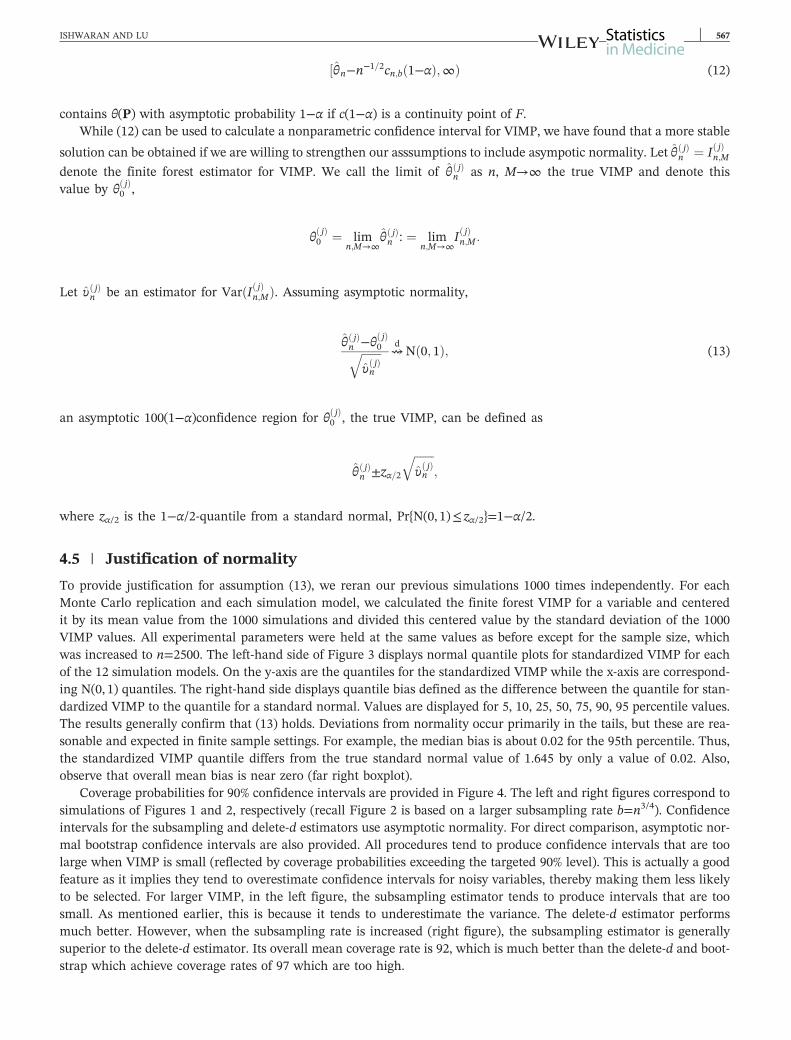
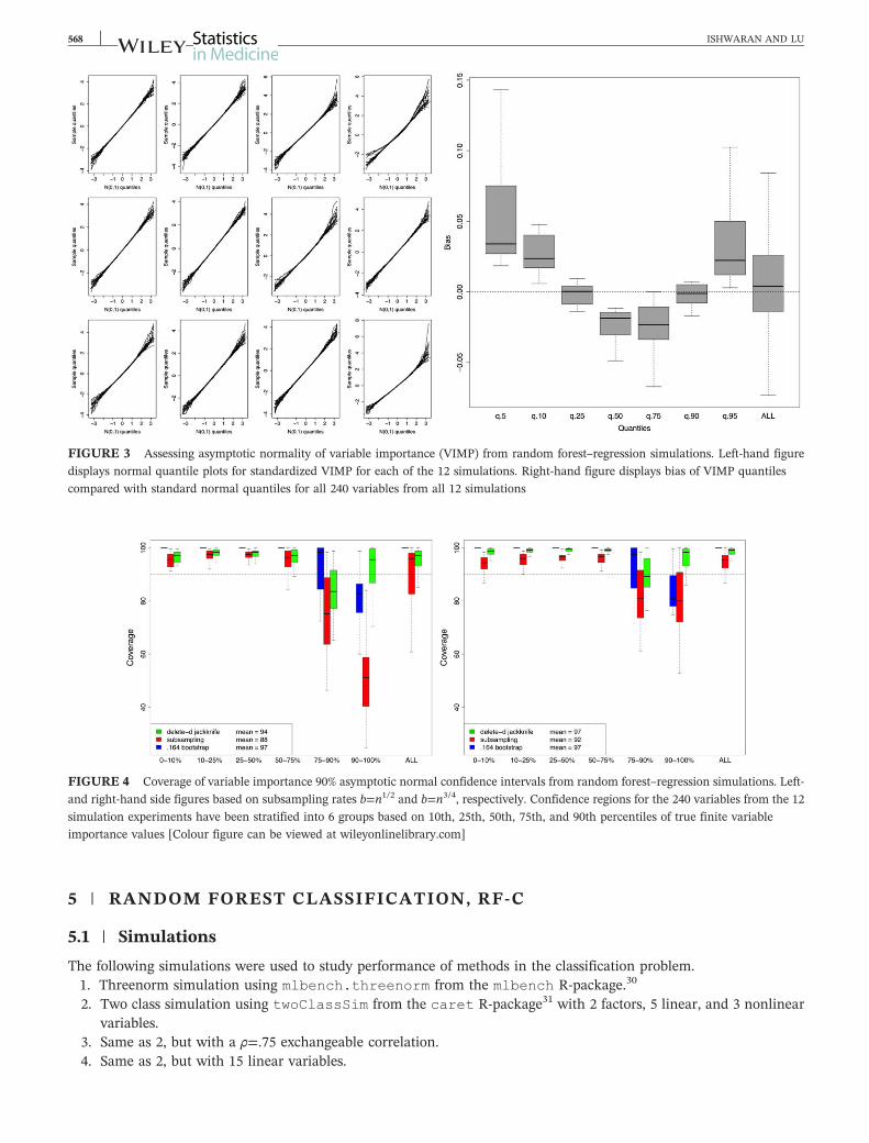
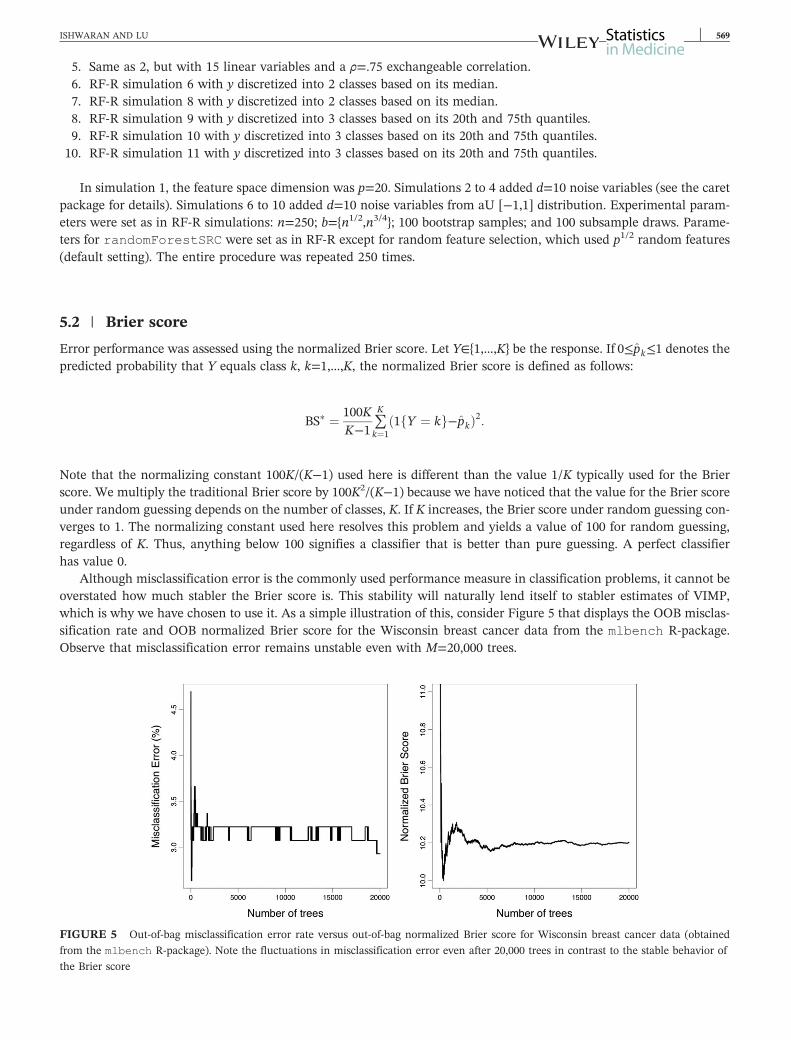
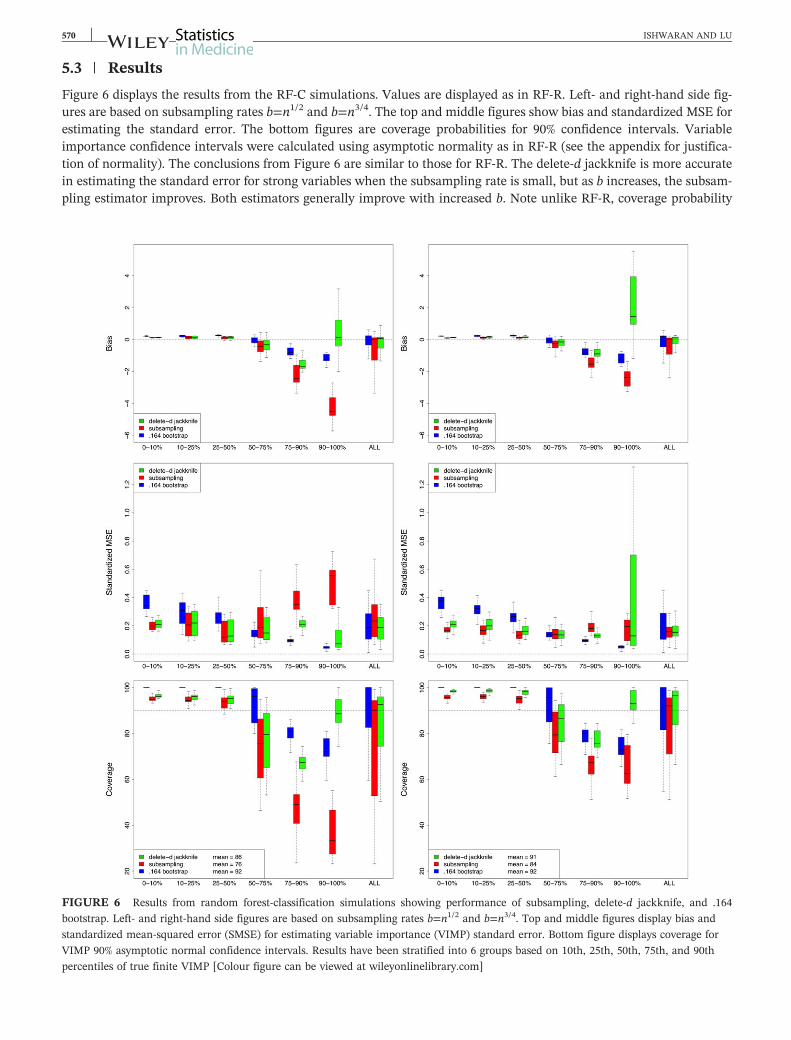
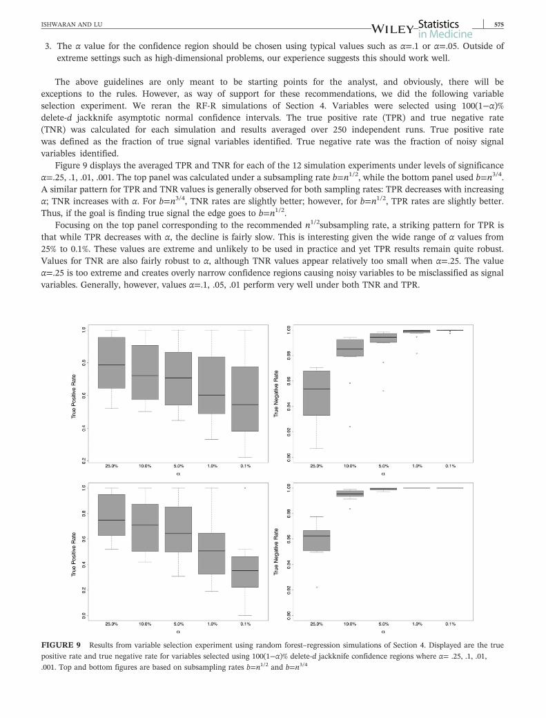ISHWARAN AND LU 559

While RFs popularity stems from its prediction performance an equally important feature is that it provides a fullynonparametric measure of variable importance (VIMP)127-9 Variable importance allows users to identify whichvariables play a key role in prediction thus providing insight into the underlying mechanism for what otherwise mightbe considered a black box We note that the concept of VIMP is not specific to RF and has a long history One of theearliest examples was CART10 which calculated VIMP by summing the reduction in node impurity due to a variableover all tree nodes Another approach calculated importance using surrogate splitting (see chapter 53 of Breimanet al10)

Early prototypes of RF software developed by Leo Breiman and his student Adele Cutler provided for variousoptions for calculating VIMP11 One procedure used for classification forests was to estimate VIMP using the forest aver-aged decrease in Gini impurity (somewhat akin to the node impurity approaches of CART) However while Gini impor-tance12 saw widespread initial use with RF over time it has become less popular8 By far the most frequently usedmeasure of importance was another measure provided by the Breiman‐Cutler software called permutation importance(sometimes also referred to as Breiman‐Cutler importance) Unlike Gini importance that estimates importance using in‐sample impurity permutation importance adopts a prediction‐based approach by using prediction error attributable tothe variable A clever feature is that rather than using cross‐validation which is computationally expensive for forestspermutation importance estimates prediction error by making use of out‐of‐bootstrap cases Recall that each tree is cal-culated from a bootstrap sample of the original data The approximately 1minus632=368 left from the bootstrap representsout‐of‐sample data which can be used for estimating prediction performance These data are called out‐of‐bag (OOB)and prediction error obtained from it is called OOB error13 Permutation importance permutes a variables OOB dataand compares the resulting OOB prediction error to the original OOB prediction errormdashthe motivation being that alarge positive value indicates a variable with predictive importance

Permutation (Breiman‐Cutler) Importance

In the OOB cases for a tree randomly permute all values of the jth variable Put these new covariate valuesdown the tree and compute a new internal error rate The amount by which this new error exceeds theoriginal OOB error is defined as the importance of the jth variable for the tree Averaging over the forestyields VIMP

mdash Measure 1 (Manual On Setting Up Using And Understanding Random Forests V31)

We focus on Breiman‐Cutler permutation importance in this manuscript (for simplicity hereafter simply referred toas VIMP) One of the tremendous advantages of VIMP is that it removes the arbitrariness of having to select a cutoffvalue when determining the effectiveness of a variable Regardless of the problem a VIMP of zero always representsan appropriate cutoff as it reflects the point at which a variable no longer contributes predictive power to the modelHowever in practice one may observe values close to zero and the meaning of what constitutes being zero becomesunclear One way to resolve this is to calculate the variance of VIMP but this is challenging due to the complex natureof RF Unfortunately while the empirical properties of VIMP are well documented14-16 much less is known aboutVIMPs theoretical properties outside of a few studies717

Given the difficulties of theoretical analysis an alternative approach is to approximate the distribution of VIMPthrough some form of resampling This has been the favored approach used for RF regression for assessing variabilityof RF predicted values Methods that have been used include bootstrapping18 for estimating the variance and the infin-itesimal jackknife19 and infinite order U‐statistics20 for confidence intervals These methods however only apply to RFpredicted values and not to VIMP which involves prediction error This greatly complicates matters and requires a moregeneral approach

For this reason we base our approach on subsampling21 a general methodology for approximating the distributionof a complex statistic Section 3 provides a description of our subsampling procedure for estimating the variance Nota-tional framework and a formal definition of VIMP are provided in Section 2 Section 3 begins by introducing a bootstrapsolution to be used as a comparison procedure Interestingly we find the bootstrap cannot be applied directly due to tiesthat occur in the OOB data This is precisely due to the fact that VIMP is prediction error based We propose a solutionto this problem called the 164 bootstrap estimator The subsampling variance estimator and the delete‐d jackknife var-iance estimator22 a close cousin are described later in Section 3 Sections 4 5 and 6 consider regression classificationand survival settings and extensively evaluate performance of the 2 subsampling methods and the 164 bootstrap

560 ISHWARAN AND LU



21 | Notation








sumM




23 | Loss function






ISHWARAN AND LU 561

24 | Tree VIMP



















sumM










562 ISHWARAN AND LU







We have



sumn

lfrac141

nminusln

n


lfrac141

nminusln

n eminus11l

l

frac14 eminus1sum

n

lfrac1411minus

ln

n1l≍eminus1sum

n

lfrac141

eminusl

l≍1635








1KsumK


THORN2



ISHWARAN AND LU 563













Qn dQ (8)



sumsisinSb


where Cb frac14 nb




sumsisinSb




υb frac14 b=nCb

sumsisinSb

θnbsminus1Cb

sumsprimeisinSb

θnbsprime

2

(10)


564 ISHWARAN AND LU


sumsisinSr




sumsisinSr

θnrsminus1Cr

sumsprimeisinSr

θnrsprime

2

thorn rd

1Cr

sumsisinSr

θnrsminusθn

2



sumsisinSb

θnbsminus1Cb

sumsprimeisinSb

θnbsprime

2

thorn bnminusb

1Cb

sumsisinSb

θnbsminusθn

2


(11)








minus1KsumK


THORN2





41 | Simulations



ISHWARAN AND LU 565









43 | Results







566 ISHWARAN AND LU








ISHWARAN AND LU 567







Ieth jTHORNnM







q












568 ISHWARAN AND LU


51 | Simulations




ISHWARAN AND LU 569



52 | Brier score



sumK






the Brier score

570 ISHWARAN AND LU

53 | Results







ISHWARAN AND LU 571




61 | Notation







GethtTHORN









572 ISHWARAN AND LU











ISHWARAN AND LU 573








574 ISHWARAN AND LU





7 | DISCUSSION

71 | Summary









ISHWARAN AND LU 575








576 ISHWARAN AND LU









ACKNOWLEDGEMENTS


ORCID


REFERENCES














ISHWARAN AND LU 577

























APPENDIX






578 ISHWARAN AND LU






Yi frac14 sump



















ISHWARAN AND LU 579









580 ISHWARAN AND LU







sumn


n

ifrac141


n

ifrac141



Similarly we have




Therefore



n






j~Rjsumiisin~R


frac14 1

j~Rjsumiisin~R


j~Rjsumiisin~R







ISHWARAN AND LU 581
















eth jTHORN ~2 ~



















n thorn oeth1THORN

582 ISHWARAN AND LU


560 ISHWARAN AND LU



21 | Notation








sumM




23 | Loss function






ISHWARAN AND LU 561

24 | Tree VIMP



















sumM










562 ISHWARAN AND LU







We have



sumn

lfrac141

nminusln

n


lfrac141

nminusln

n eminus11l

l

frac14 eminus1sum

n

lfrac1411minus

ln

n1l≍eminus1sum

n

lfrac141

eminusl

l≍1635








1KsumK


THORN2



ISHWARAN AND LU 563













Qn dQ (8)



sumsisinSb


where Cb frac14 nb




sumsisinSb




υb frac14 b=nCb

sumsisinSb

θnbsminus1Cb

sumsprimeisinSb

θnbsprime

2

(10)


564 ISHWARAN AND LU


sumsisinSr




sumsisinSr

θnrsminus1Cr

sumsprimeisinSr

θnrsprime

2

thorn rd

1Cr

sumsisinSr

θnrsminusθn

2



sumsisinSb

θnbsminus1Cb

sumsprimeisinSb

θnbsprime

2

thorn bnminusb

1Cb

sumsisinSb

θnbsminusθn

2


(11)








minus1KsumK


THORN2





41 | Simulations



ISHWARAN AND LU 565









43 | Results







566 ISHWARAN AND LU








ISHWARAN AND LU 567







Ieth jTHORNnM







q












568 ISHWARAN AND LU


51 | Simulations




ISHWARAN AND LU 569



52 | Brier score



sumK






the Brier score

570 ISHWARAN AND LU

53 | Results







ISHWARAN AND LU 571




61 | Notation







GethtTHORN









572 ISHWARAN AND LU











ISHWARAN AND LU 573








574 ISHWARAN AND LU





7 | DISCUSSION

71 | Summary









ISHWARAN AND LU 575








576 ISHWARAN AND LU









ACKNOWLEDGEMENTS


ORCID


REFERENCES














ISHWARAN AND LU 577

























APPENDIX






578 ISHWARAN AND LU






Yi frac14 sump



















ISHWARAN AND LU 579









580 ISHWARAN AND LU







sumn


n

ifrac141


n

ifrac141



Similarly we have




Therefore



n






j~Rjsumiisin~R


frac14 1

j~Rjsumiisin~R


j~Rjsumiisin~R







ISHWARAN AND LU 581
















eth jTHORN ~2 ~



















n thorn oeth1THORN

582 ISHWARAN AND LU


ISHWARAN AND LU 561

24 | Tree VIMP



















sumM










562 ISHWARAN AND LU







We have



sumn

lfrac141

nminusln

n


lfrac141

nminusln

n eminus11l

l

frac14 eminus1sum

n

lfrac1411minus

ln

n1l≍eminus1sum

n

lfrac141

eminusl

l≍1635








1KsumK


THORN2



ISHWARAN AND LU 563













Qn dQ (8)



sumsisinSb


where Cb frac14 nb




sumsisinSb




υb frac14 b=nCb

sumsisinSb

θnbsminus1Cb

sumsprimeisinSb

θnbsprime

2

(10)


564 ISHWARAN AND LU


sumsisinSr




sumsisinSr

θnrsminus1Cr

sumsprimeisinSr

θnrsprime

2

thorn rd

1Cr

sumsisinSr

θnrsminusθn

2



sumsisinSb

θnbsminus1Cb

sumsprimeisinSb

θnbsprime

2

thorn bnminusb

1Cb

sumsisinSb

θnbsminusθn

2


(11)








minus1KsumK


THORN2





41 | Simulations



ISHWARAN AND LU 565









43 | Results







566 ISHWARAN AND LU








ISHWARAN AND LU 567







Ieth jTHORNnM







q












568 ISHWARAN AND LU


51 | Simulations




ISHWARAN AND LU 569



52 | Brier score



sumK






the Brier score

570 ISHWARAN AND LU

53 | Results







ISHWARAN AND LU 571




61 | Notation







GethtTHORN









572 ISHWARAN AND LU











ISHWARAN AND LU 573








574 ISHWARAN AND LU





7 | DISCUSSION

71 | Summary









ISHWARAN AND LU 575








576 ISHWARAN AND LU









ACKNOWLEDGEMENTS


ORCID


REFERENCES














ISHWARAN AND LU 577

























APPENDIX






578 ISHWARAN AND LU






Yi frac14 sump



















ISHWARAN AND LU 579









580 ISHWARAN AND LU







sumn


n

ifrac141


n

ifrac141



Similarly we have




Therefore



n






j~Rjsumiisin~R


frac14 1

j~Rjsumiisin~R


j~Rjsumiisin~R







ISHWARAN AND LU 581
















eth jTHORN ~2 ~



















n thorn oeth1THORN

582 ISHWARAN AND LU


562 ISHWARAN AND LU







We have



sumn

lfrac141

nminusln

n


lfrac141

nminusln

n eminus11l

l

frac14 eminus1sum

n

lfrac1411minus

ln

n1l≍eminus1sum

n

lfrac141

eminusl

l≍1635








1KsumK


THORN2



ISHWARAN AND LU 563













Qn dQ (8)



sumsisinSb


where Cb frac14 nb




sumsisinSb




υb frac14 b=nCb

sumsisinSb

θnbsminus1Cb

sumsprimeisinSb

θnbsprime

2

(10)


564 ISHWARAN AND LU


sumsisinSr




sumsisinSr

θnrsminus1Cr

sumsprimeisinSr

θnrsprime

2

thorn rd

1Cr

sumsisinSr

θnrsminusθn

2



sumsisinSb

θnbsminus1Cb

sumsprimeisinSb

θnbsprime

2

thorn bnminusb

1Cb

sumsisinSb

θnbsminusθn

2


(11)








minus1KsumK


THORN2





41 | Simulations



ISHWARAN AND LU 565









43 | Results







566 ISHWARAN AND LU








ISHWARAN AND LU 567







Ieth jTHORNnM







q












568 ISHWARAN AND LU


51 | Simulations




ISHWARAN AND LU 569



52 | Brier score



sumK






the Brier score

570 ISHWARAN AND LU

53 | Results







ISHWARAN AND LU 571




61 | Notation







GethtTHORN









572 ISHWARAN AND LU











ISHWARAN AND LU 573








574 ISHWARAN AND LU





7 | DISCUSSION

71 | Summary









ISHWARAN AND LU 575








576 ISHWARAN AND LU









ACKNOWLEDGEMENTS


ORCID


REFERENCES














ISHWARAN AND LU 577

























APPENDIX






578 ISHWARAN AND LU






Yi frac14 sump



















ISHWARAN AND LU 579









580 ISHWARAN AND LU







sumn


n

ifrac141


n

ifrac141



Similarly we have




Therefore



n






j~Rjsumiisin~R


frac14 1

j~Rjsumiisin~R


j~Rjsumiisin~R







ISHWARAN AND LU 581
















eth jTHORN ~2 ~



















n thorn oeth1THORN

582 ISHWARAN AND LU


ISHWARAN AND LU 563













Qn dQ (8)



sumsisinSb


where Cb frac14 nb




sumsisinSb




υb frac14 b=nCb

sumsisinSb

θnbsminus1Cb

sumsprimeisinSb

θnbsprime

2

(10)


564 ISHWARAN AND LU


sumsisinSr




sumsisinSr

θnrsminus1Cr

sumsprimeisinSr

θnrsprime

2

thorn rd

1Cr

sumsisinSr

θnrsminusθn

2



sumsisinSb

θnbsminus1Cb

sumsprimeisinSb

θnbsprime

2

thorn bnminusb

1Cb

sumsisinSb

θnbsminusθn

2


(11)








minus1KsumK


THORN2





41 | Simulations



ISHWARAN AND LU 565









43 | Results







566 ISHWARAN AND LU








ISHWARAN AND LU 567







Ieth jTHORNnM







q












568 ISHWARAN AND LU


51 | Simulations




ISHWARAN AND LU 569



52 | Brier score



sumK






the Brier score

570 ISHWARAN AND LU

53 | Results







ISHWARAN AND LU 571




61 | Notation







GethtTHORN









572 ISHWARAN AND LU











ISHWARAN AND LU 573








574 ISHWARAN AND LU





7 | DISCUSSION

71 | Summary









ISHWARAN AND LU 575








576 ISHWARAN AND LU









ACKNOWLEDGEMENTS


ORCID


REFERENCES














ISHWARAN AND LU 577

























APPENDIX






578 ISHWARAN AND LU






Yi frac14 sump



















ISHWARAN AND LU 579









580 ISHWARAN AND LU







sumn


n

ifrac141


n

ifrac141



Similarly we have




Therefore



n






j~Rjsumiisin~R


frac14 1

j~Rjsumiisin~R


j~Rjsumiisin~R







ISHWARAN AND LU 581
















eth jTHORN ~2 ~



















n thorn oeth1THORN

582 ISHWARAN AND LU


564 ISHWARAN AND LU


sumsisinSr




sumsisinSr

θnrsminus1Cr

sumsprimeisinSr

θnrsprime

2

thorn rd

1Cr

sumsisinSr

θnrsminusθn

2



sumsisinSb

θnbsminus1Cb

sumsprimeisinSb

θnbsprime

2

thorn bnminusb

1Cb

sumsisinSb

θnbsminusθn

2


(11)








minus1KsumK


THORN2





41 | Simulations



ISHWARAN AND LU 565









43 | Results







566 ISHWARAN AND LU








ISHWARAN AND LU 567







Ieth jTHORNnM







q












568 ISHWARAN AND LU


51 | Simulations




ISHWARAN AND LU 569



52 | Brier score



sumK






the Brier score

570 ISHWARAN AND LU

53 | Results







ISHWARAN AND LU 571




61 | Notation







GethtTHORN









572 ISHWARAN AND LU











ISHWARAN AND LU 573








574 ISHWARAN AND LU





7 | DISCUSSION

71 | Summary









ISHWARAN AND LU 575








576 ISHWARAN AND LU









ACKNOWLEDGEMENTS


ORCID


REFERENCES














ISHWARAN AND LU 577

























APPENDIX






578 ISHWARAN AND LU






Yi frac14 sump



















ISHWARAN AND LU 579









580 ISHWARAN AND LU







sumn


n

ifrac141


n

ifrac141



Similarly we have




Therefore



n






j~Rjsumiisin~R


frac14 1

j~Rjsumiisin~R


j~Rjsumiisin~R







ISHWARAN AND LU 581
















eth jTHORN ~2 ~



















n thorn oeth1THORN

582 ISHWARAN AND LU


ISHWARAN AND LU 565









43 | Results







566 ISHWARAN AND LU








ISHWARAN AND LU 567







Ieth jTHORNnM







q












568 ISHWARAN AND LU


51 | Simulations




ISHWARAN AND LU 569



52 | Brier score



sumK






the Brier score

570 ISHWARAN AND LU

53 | Results







ISHWARAN AND LU 571




61 | Notation







GethtTHORN









572 ISHWARAN AND LU











ISHWARAN AND LU 573








574 ISHWARAN AND LU





7 | DISCUSSION

71 | Summary









ISHWARAN AND LU 575








576 ISHWARAN AND LU









ACKNOWLEDGEMENTS


ORCID


REFERENCES














ISHWARAN AND LU 577

























APPENDIX






578 ISHWARAN AND LU






Yi frac14 sump



















ISHWARAN AND LU 579









580 ISHWARAN AND LU







sumn


n

ifrac141


n

ifrac141



Similarly we have




Therefore



n






j~Rjsumiisin~R


frac14 1

j~Rjsumiisin~R


j~Rjsumiisin~R







ISHWARAN AND LU 581
















eth jTHORN ~2 ~



















n thorn oeth1THORN

582 ISHWARAN AND LU






566 ISHWARAN AND LU








ISHWARAN AND LU 567







Ieth jTHORNnM







q












568 ISHWARAN AND LU


51 | Simulations




ISHWARAN AND LU 569



52 | Brier score



sumK






the Brier score

570 ISHWARAN AND LU

53 | Results







ISHWARAN AND LU 571




61 | Notation







GethtTHORN









572 ISHWARAN AND LU











ISHWARAN AND LU 573








574 ISHWARAN AND LU





7 | DISCUSSION

71 | Summary









ISHWARAN AND LU 575








576 ISHWARAN AND LU









ACKNOWLEDGEMENTS


ORCID


REFERENCES














ISHWARAN AND LU 577

























APPENDIX






578 ISHWARAN AND LU






Yi frac14 sump



















ISHWARAN AND LU 579









580 ISHWARAN AND LU







sumn


n

ifrac141


n

ifrac141



Similarly we have




Therefore



n






j~Rjsumiisin~R


frac14 1

j~Rjsumiisin~R


j~Rjsumiisin~R







ISHWARAN AND LU 581
















eth jTHORN ~2 ~



















n thorn oeth1THORN

582 ISHWARAN AND LU


ISHWARAN AND LU 567







Ieth jTHORNnM







q












568 ISHWARAN AND LU


51 | Simulations




ISHWARAN AND LU 569



52 | Brier score



sumK






the Brier score

570 ISHWARAN AND LU

53 | Results







ISHWARAN AND LU 571




61 | Notation







GethtTHORN









572 ISHWARAN AND LU











ISHWARAN AND LU 573








574 ISHWARAN AND LU





7 | DISCUSSION

71 | Summary









ISHWARAN AND LU 575








576 ISHWARAN AND LU









ACKNOWLEDGEMENTS


ORCID


REFERENCES














ISHWARAN AND LU 577

























APPENDIX






578 ISHWARAN AND LU






Yi frac14 sump



















ISHWARAN AND LU 579









580 ISHWARAN AND LU







sumn


n

ifrac141


n

ifrac141



Similarly we have




Therefore



n






j~Rjsumiisin~R


frac14 1

j~Rjsumiisin~R


j~Rjsumiisin~R







ISHWARAN AND LU 581
















eth jTHORN ~2 ~



















n thorn oeth1THORN

582 ISHWARAN AND LU









568 ISHWARAN AND LU


51 | Simulations




ISHWARAN AND LU 569



52 | Brier score



sumK






the Brier score

570 ISHWARAN AND LU

53 | Results







ISHWARAN AND LU 571




61 | Notation







GethtTHORN









572 ISHWARAN AND LU











ISHWARAN AND LU 573








574 ISHWARAN AND LU





7 | DISCUSSION

71 | Summary









ISHWARAN AND LU 575








576 ISHWARAN AND LU









ACKNOWLEDGEMENTS


ORCID


REFERENCES














ISHWARAN AND LU 577

























APPENDIX






578 ISHWARAN AND LU






Yi frac14 sump



















ISHWARAN AND LU 579









580 ISHWARAN AND LU







sumn


n

ifrac141


n

ifrac141



Similarly we have




Therefore



n






j~Rjsumiisin~R


frac14 1

j~Rjsumiisin~R


j~Rjsumiisin~R







ISHWARAN AND LU 581
















eth jTHORN ~2 ~



















n thorn oeth1THORN

582 ISHWARAN AND LU


ISHWARAN AND LU 569



52 | Brier score



sumK






the Brier score

570 ISHWARAN AND LU

53 | Results







ISHWARAN AND LU 571




61 | Notation







GethtTHORN









572 ISHWARAN AND LU











ISHWARAN AND LU 573








574 ISHWARAN AND LU





7 | DISCUSSION

71 | Summary









ISHWARAN AND LU 575








576 ISHWARAN AND LU









ACKNOWLEDGEMENTS


ORCID


REFERENCES














ISHWARAN AND LU 577

























APPENDIX






578 ISHWARAN AND LU






Yi frac14 sump



















ISHWARAN AND LU 579









580 ISHWARAN AND LU







sumn


n

ifrac141


n

ifrac141



Similarly we have




Therefore



n






j~Rjsumiisin~R


frac14 1

j~Rjsumiisin~R


j~Rjsumiisin~R







ISHWARAN AND LU 581
















eth jTHORN ~2 ~



















n thorn oeth1THORN

582 ISHWARAN AND LU


570 ISHWARAN AND LU

53 | Results







ISHWARAN AND LU 571




61 | Notation







GethtTHORN









572 ISHWARAN AND LU











ISHWARAN AND LU 573








574 ISHWARAN AND LU





7 | DISCUSSION

71 | Summary









ISHWARAN AND LU 575








576 ISHWARAN AND LU









ACKNOWLEDGEMENTS


ORCID


REFERENCES














ISHWARAN AND LU 577

























APPENDIX






578 ISHWARAN AND LU






Yi frac14 sump



















ISHWARAN AND LU 579









580 ISHWARAN AND LU







sumn


n

ifrac141


n

ifrac141



Similarly we have




Therefore



n






j~Rjsumiisin~R


frac14 1

j~Rjsumiisin~R


j~Rjsumiisin~R







ISHWARAN AND LU 581
















eth jTHORN ~2 ~



















n thorn oeth1THORN

582 ISHWARAN AND LU


ISHWARAN AND LU 571




61 | Notation







GethtTHORN









572 ISHWARAN AND LU











ISHWARAN AND LU 573








574 ISHWARAN AND LU





7 | DISCUSSION

71 | Summary









ISHWARAN AND LU 575








576 ISHWARAN AND LU









ACKNOWLEDGEMENTS


ORCID


REFERENCES














ISHWARAN AND LU 577

























APPENDIX






578 ISHWARAN AND LU






Yi frac14 sump



















ISHWARAN AND LU 579









580 ISHWARAN AND LU







sumn


n

ifrac141


n

ifrac141



Similarly we have




Therefore



n






j~Rjsumiisin~R


frac14 1

j~Rjsumiisin~R


j~Rjsumiisin~R







ISHWARAN AND LU 581
















eth jTHORN ~2 ~



















n thorn oeth1THORN

582 ISHWARAN AND LU


572 ISHWARAN AND LU











ISHWARAN AND LU 573








574 ISHWARAN AND LU





7 | DISCUSSION

71 | Summary









ISHWARAN AND LU 575








576 ISHWARAN AND LU









ACKNOWLEDGEMENTS


ORCID


REFERENCES














ISHWARAN AND LU 577

























APPENDIX






578 ISHWARAN AND LU






Yi frac14 sump



















ISHWARAN AND LU 579









580 ISHWARAN AND LU







sumn


n

ifrac141


n

ifrac141



Similarly we have




Therefore



n






j~Rjsumiisin~R


frac14 1

j~Rjsumiisin~R


j~Rjsumiisin~R







ISHWARAN AND LU 581
















eth jTHORN ~2 ~



















n thorn oeth1THORN

582 ISHWARAN AND LU


ISHWARAN AND LU 573








574 ISHWARAN AND LU





7 | DISCUSSION

71 | Summary









ISHWARAN AND LU 575








576 ISHWARAN AND LU









ACKNOWLEDGEMENTS


ORCID


REFERENCES














ISHWARAN AND LU 577

























APPENDIX






578 ISHWARAN AND LU






Yi frac14 sump



















ISHWARAN AND LU 579









580 ISHWARAN AND LU







sumn


n

ifrac141


n

ifrac141



Similarly we have




Therefore



n






j~Rjsumiisin~R


frac14 1

j~Rjsumiisin~R


j~Rjsumiisin~R







ISHWARAN AND LU 581
















eth jTHORN ~2 ~



















n thorn oeth1THORN

582 ISHWARAN AND LU


574 ISHWARAN AND LU





7 | DISCUSSION

71 | Summary









ISHWARAN AND LU 575








576 ISHWARAN AND LU









ACKNOWLEDGEMENTS


ORCID


REFERENCES














ISHWARAN AND LU 577

























APPENDIX






578 ISHWARAN AND LU






Yi frac14 sump



















ISHWARAN AND LU 579









580 ISHWARAN AND LU







sumn


n

ifrac141


n

ifrac141



Similarly we have




Therefore



n






j~Rjsumiisin~R


frac14 1

j~Rjsumiisin~R


j~Rjsumiisin~R







ISHWARAN AND LU 581
















eth jTHORN ~2 ~



















n thorn oeth1THORN

582 ISHWARAN AND LU


ISHWARAN AND LU 575








576 ISHWARAN AND LU









ACKNOWLEDGEMENTS


ORCID


REFERENCES














ISHWARAN AND LU 577

























APPENDIX






578 ISHWARAN AND LU






Yi frac14 sump



















ISHWARAN AND LU 579









580 ISHWARAN AND LU







sumn


n

ifrac141


n

ifrac141



Similarly we have




Therefore



n






j~Rjsumiisin~R


frac14 1

j~Rjsumiisin~R


j~Rjsumiisin~R







ISHWARAN AND LU 581
















eth jTHORN ~2 ~



















n thorn oeth1THORN

582 ISHWARAN AND LU


576 ISHWARAN AND LU









ACKNOWLEDGEMENTS


ORCID


REFERENCES














ISHWARAN AND LU 577

























APPENDIX






578 ISHWARAN AND LU






Yi frac14 sump



















ISHWARAN AND LU 579









580 ISHWARAN AND LU







sumn


n

ifrac141


n

ifrac141



Similarly we have




Therefore



n






j~Rjsumiisin~R


frac14 1

j~Rjsumiisin~R


j~Rjsumiisin~R







ISHWARAN AND LU 581
















eth jTHORN ~2 ~



















n thorn oeth1THORN

582 ISHWARAN AND LU


ISHWARAN AND LU 577

























APPENDIX






578 ISHWARAN AND LU






Yi frac14 sump



















ISHWARAN AND LU 579









580 ISHWARAN AND LU







sumn


n

ifrac141


n

ifrac141



Similarly we have




Therefore



n






j~Rjsumiisin~R


frac14 1

j~Rjsumiisin~R


j~Rjsumiisin~R







ISHWARAN AND LU 581
















eth jTHORN ~2 ~



















n thorn oeth1THORN

582 ISHWARAN AND LU





578 ISHWARAN AND LU






Yi frac14 sump



















ISHWARAN AND LU 579









580 ISHWARAN AND LU







sumn


n

ifrac141


n

ifrac141



Similarly we have




Therefore



n






j~Rjsumiisin~R


frac14 1

j~Rjsumiisin~R


j~Rjsumiisin~R







ISHWARAN AND LU 581
















eth jTHORN ~2 ~



















n thorn oeth1THORN

582 ISHWARAN AND LU







ISHWARAN AND LU 579









580 ISHWARAN AND LU







sumn


n

ifrac141


n

ifrac141



Similarly we have




Therefore



n






j~Rjsumiisin~R


frac14 1

j~Rjsumiisin~R


j~Rjsumiisin~R







ISHWARAN AND LU 581
















eth jTHORN ~2 ~



















n thorn oeth1THORN

582 ISHWARAN AND LU


580 ISHWARAN AND LU







sumn


n

ifrac141


n

ifrac141



Similarly we have




Therefore



n






j~Rjsumiisin~R


frac14 1

j~Rjsumiisin~R


j~Rjsumiisin~R







ISHWARAN AND LU 581
















eth jTHORN ~2 ~



















n thorn oeth1THORN

582 ISHWARAN AND LU


ISHWARAN AND LU 581
















eth jTHORN ~2 ~



















n thorn oeth1THORN

582 ISHWARAN AND LU


582 ISHWARAN AND LU


standard errors and confidence ... - web.ccs.miami.edu

Documents