staff.math.su.sestaff.math.su.se/kurasov/pdfarchiv/naboko12-kluwer.pdf · mathematical physics,...

Mathematical Physics, Analysis and Geometry 5: 243–286, 2002.© 2002 Kluwer Academic Publishers. Printed in the Netherlands.

243

On the Essential Spectrum of a Class of SingularMatrix Differential Operators. I: QuasiregularityConditions and Essential Self-adjointness

PAVEL KURASOV1 and SERGUEI NABOKO2

1Dept. of Mathematics, Lund Institute of Technology, Box 118, 221 00 Lund, Sweden.e-mail: [email protected]. of Mathematical Physics, St. Petersburg Univ., 198904 St. Petersburg, Russia.e-mail: [email protected]

(Received: 5 December 2001; in final form: 26 August 2002)

Abstract. The essential spectrum of singular matrix differential operator determined by the operatormatrix

− ddx ρ(x)

ddx + q(x) d

dxβx

−βx

ddx

m(x)

x2

is studied. It is proven that the essential spectrum of any self-adjoint operator associated with thisexpression consists of two branches. One of these branches (called regularity spectrum) can beobtained by approximating the operator by regular operators (with coefficients which are boundednear the origin), the second branch (called singularity spectrum) appears due to singularity of thecoefficients.

Mathematics Subject Classifications (2000): Primary: 47A10, 76W05; secondary: 34L05, 47B25.

Key words: essential spectrum, quasiregularity conditions, Hain–Lüst operator.

1. Introduction

Systems of ordinary and partial differential and pseudodifferential equations is asubject of interest for many mathematicians (see [19] and numerous referencestherein). Matrix ordinary differential operators of mixed order appear in manyproblems of theoretical physics: hydrodynamics, plasma physics, quantum fieldtheory, and others. Mathematically rigorous treatment of such problems has beencarried out by several authors: J. A. Adam, V. Adamyan, J. Descluox, G. Gey-monat, G. Grubb, T. Kako, H. Langer, A. E. Lifchitz, R. Mennicken, M. Möller,G. D. Raikov, A. Shkalikov, and others [1, 2, 4, 5, 8–11, 15, 17, 20–23, 28, 29, 31,37]. Matrix differential operators with singular coefficients are of special interestin plasma physics, for example so-called force operators describing equilibriumstate of plasma in toroidal region are exactly of this kind [20]. A more general

244 PAVEL KURASOV AND SERGUEI NABOKO

class of 3 × 3 matrix differential operators with singularities was considered byV. Hardt, R. Mennicken, and S. Naboko [17], where a new branch of the essentialspectrum determined by the singularity was observed and described. This newbranch had been predicted by J. Descloux and G. Geymonat [5]. To study theessential spectrum of the operator, so-called quasiregularity conditions were intro-duced ([17]). These conditions are necessary and sufficient for the boundednessof the essential spectrum of the singular operator. A different approach to thisclass of matrix operators satisfying the quasiregularity conditions was developedby M. Faierman, R. Mennicken, and M. Möller [10]. Recently, R. Mennicken,S. Naboko, and Ch. Tretter suggested clarifying approach to study this class ofsingular operators ([30]). It was discovered that the new branch of the essentialspectrum can be characterized as the zero set for the symbol of the asymptoticHain–Lüst operator introduced in [30]. It should be mentioned that in the newapproach, the authors used Proposition A.1 from the current paper.

Investigation of the essential spectrum of differential and partial differential op-erators attracts attention of many scientists ([40, 41, 44]). For example the spectrumof pseudodifferential operators with piecewise continuous symbols has been inves-tigated by S. C. Power [35, 36]. In [14] (Chapter 3), it is shown how to calculatethe essential spectrum for pseudodifferential boundary value problems using theprincipal interior and boundary symbol operators.

A new class of matrix differential operators with singular coefficients is intro-duced and investigated in this paper. This class consists of 2×2 matrices instead ofthe 3 × 3 operator matrices studied in [30], which is a formal simplification. (Themethod elaborated in the paper can be applied to m × m operator matrices.) Butall essential features of the problem are still present. Additionally the singularitiesof the matrix elements are distributed in a different way. We decided to study thisclass of singular operators in order to illustrate the mechanism of the appearanceof the additional branch of essential spectrum using the most explicit example.This helps us to avoid tedious calculations and at the same time preserves themain features of the original problem. For this reason we tried to develop a properCalkin calculus (see Appendix B), which allows one to justify calculations from[17, 20–22] being incomplete. On the other hand, employment of Calkin calculusmakes all calculations transparent and easier. For example, the authors of [4], in-vestigating nonsingular operator matrices, used subtle results from operator theorydue to P. E. Sobolevskii [26]. Developing these methods, some new results onBanach space operators were obtained. These results on the spectrum of the sumof three operators are of an abstract nature and can be used in other problems aswell. Investigating this problem, we tried to elaborate a new general approach tosingular matrix differential operators. We hope to be able to apply this methodto most general singular matrix differential operators including partial differentialoperators.

The operator under investigation is determined formally by the following ex-pression:

ON THE ESSENTIAL SPECTRUM OF MATRIX DIFFERENTIAL OPERATORS I 245

− d

dxρ(x)

d

dx+ q(x) d

dx

β

x

−βx

d

dx

m(x)

x2

. (1)

We use this form of the matrix differential operator in order to display explicitlythe singularities of three matrix elements at the origin. The most interesting (andcomplicated) case is when the functions β and m do not vanish at the origin.Therefore, the operator defined by the functions β andm having zeroes at the originof order 1 and 2 respectively, will be called regular. In this case, all singularitiesare artificial. The essential spectrum of the corresponding operator can easily beinvestigated using the methods of [4]. All other operators from the described classwill be called singular and we are going to concentrate our attention on the caseof singular operators only. It is clear that the matrix symbol does not determine theself-adjoint operator uniquely even in the regular case. The extension theory, of theminimal operator in the regular case has been developed by H. de Snoo [43] and inthe case of nonsingular leading matrix coefficient in [38, 39].

Our interest in singular problem is motivated by the new spectral phenomenonwhich can be observed in this case: the essential spectrum of any selfadjoint op-erator corresponding to the symbol (1) in L2[0, 1] ⊕ L2[0, 1] cannot be describedas a limit of the essential spectra of the operators determined by the same symbolin L2[ε, 1] ⊕ L2[ε, 1] as ε → +0. Such limit determines only a certain part ofthe essential spectrum of the operator in L2[0, 1] ⊕ L2[0, 1]. An additional branchof the essential spectrum appears due to the singularity of the coefficients at theorigin. Trivial counterpart of this phenomena is well known for infinite intervals,since for example the essential spectrum of −(d2/dx2) on a finite interval [−an, bn]is empty and therefore does not give the essential spectrum of −(d2/dx2) on thewhole line when an, bn → ∞. The phenomenon described in the current note ismore sophisticated and is due to rather complicated interplay between the com-ponents of the matrix differential operator. On the other hand, the coefficient ofthe matrix determining the operator have singularities at the boundary points. Thisnew branch of essential spectrum is absent in the case of regular operators, sincethe limit procedure for the essential spectrum described above gives the correctanswer in the regular case. Spectral analysis in the regular case is well knownand can be carried out using methods developed in [4, 15]. In what follows, thetwo branches of the essential spectrum will be called the regularity spectrum andsingularity spectrum, respectively. We introduce quasiregularity conditions for thesingular operator which guarantees boundedness of the regularity spectrum. Thequasiregularity conditions determine a special class of singular matrix differen-tial operators for which we are able to calculate the essential spectra. Note thatin many physical applications, i.e. in plasma physics ([20]), these conditions arefulfilled.

The singularities of the operator coefficients at the origin play an important roleeven at the stage of the definition of the self-adjoint operator corresponding to the


formal expression (1). The indices of the minimal differential operator producedby the singular point are investigated by considering the extension of the minimaloperator to the set of functions satisfying certain symmetric boundary condition atthe regular point. (In this way the singular x = 0 and regular x = 1 endpointsare treated separately and in different ways.) It is proven that this extended op-erator has trivial deficiency indices (is essentially self-adjoint) if and only if thequasiregularity conditions are satisfied and β(0) = 0. (The condition β(0) = 0together with the quasiregularity condition (8) imply for smooth coefficients thatm(0) = m′(0) = 0 and therefore that the operator L is not singular.) If at leastone of the quasiregularity conditions is not satisfied or the function β vanishesat the origin then the deficiency indices of the described extended operator arenontrivial like it is in the regular case. We would like to note that the quasiregularityconditions introduced originally to guarantee boundedness of the regular branch ofthe essential spectrum play an important role in the investigation of the deficiencyindices. (Note that the name quasiregularity conditions has nothing to do withthe regularity of the extension problem for the operator. It refers to the essentialspectrum only.)

After the family of self-adjoint operators corresponding to the formal expres-sion (1) is determined, we discuss the transformation of the operator using theexponential map of the interval [0, 1] onto the half-infinite interval [0,∞). Thismap transforms the singular point at the origin to a point at ∞ and enables us touse the standard Fourier transform in L2(R). So the reason to use this exponentialmap is pure technical.

Since we are interested in the essential spectrum of the corresponding self-adjoint operators, the choice of the boundary conditions in the limit circle caseis not important. The difference between the resolvents of any two operators fromthis family is a finite rank operator. To calculate the essential spectrum of anysuch selfadjoint operator we use the even stronger fact that the essential spectra ofany two self-adjoint operators coincide if the difference between their resolvents iscompact (Weyl theorem). We develop a so-called cleaning procedure which enablesone to reduce the calculation of the essential spectrum of the complicated matrixdifferential operator given by (1) to the calculation of the essential spectrum of acertain asymptotic singular operator with real coefficients. The singular coefficientsof the asymptotic operator are chosen to have the same singularities as those of theoriginal operator. In other words the asymptotic operator is chosen so that the dif-ference between the resolvents of the original and asymptotic operators is compact.The Hain–Lüst operator can be considered as a regularized determinant of the 2×2matrix differential operator (1), and it plays a very important role in the cleaningprocedure. In the considered case the Hain–Lüst operator is an ordinary (scalar)second order differential operator in L2(R+). We hope that the approach developedin the current paper can be applied to more general operators including arbitrarydimension matrix differential operators and matrix partial differential operators.The method of cleaning of the resolvent modulo compact operators is of general


nature. Several abstract lemmas proven in the present paper can be applied withouteven minor changes.

To calculate the essential spectrum of the asymptotic operator we use the factthat its resolvent is equal to the separable sum of two pseudodifferential operators.We call the sum of two pseudodifferential operators separable if the symbol ofone of these two operators depends only on the space variable, and the symbolof the other operator depends only on the momentum variable. Calculation of theessential spectrum of such operators is based on Proposition A.1 from Appendix A.

We observe that the essential spectrum of the model operator under consider-ation coincides with the set of zeroes of the symbol of the asymptotic Hain–Lüstoperator. That operator is a modified version of the original Hain–Lüst operatorwhich preserves information on the behavior of the coefficients at the singular pointonly. This operator has a more simple expression: it is a second-order differentialoperator with constant coefficients. Unfortunately all information concerning theregularity spectrum disappears during this rectification. This probably general re-lation between the symbol of the asymptotic Hain–Lüst operator and the singularityspectrum will be investigated in one of the forthcoming publications.

The methods developed in this article can easily be extended to include differen-tial operators determined by operator matrices of higher dimension. For example,the case when the coefficient m appearing in (1) is a matrix can easily be investi-gated. The developed methods can help to study matrix partial differential operatorsas well. These subjects will be discussed in a future publication.

2. The Minimal Operator

Let us consider the linear operator defined by the following operator valued 2 × 2matrix

L :=

− d

dxρ(x)

d

dx+ q(x) d

dx

β

x

−βx

d

dx

m(x)

x2

, (2)

where the real-valued functions ρ(x), q(x), β(x), and m(x) are continuously dif-ferentiable in the closed interval [0, 1]

ρ, q, β,m ∈ C2[0, 1]. (3)

In addition we suppose that the density function ρ is positive (definite)

ρ(x) � ρ0 > 0. (4)

Certainly these conditions on the coefficients are far from being necessary for ouranalysis, but we assume these conditions in order to avoid unnecessary complica-tions. In this way we are able to present certain new ideas explicitly without gettingthe most optimal result.


The operator matrix (2) determines rather complicated matrix differential op-erator. Indeed in its formal determinant which controls the spectrum of the wholeoperator the differential order of the formal product of the diagonal elements(

− d

dxρ(x)

d

dx+ q(x)

)m(x)

x2

coincides with that of the formal product of the antidiagonal elements

d

dx

β

x

(−βx

d

dx

).

The same holds true for the orders of the singularities at the origin. These relationscan be expressed by the diagrams 2 + 0 = 1 + 1 for the order of differentialoperators and 0 + 2 = 1 + 1 for the orders of the power-like singularities at theorigin. These conditions imply that the nondiagonal coupling cannot be consideredas a weak perturbation of the diagonal part of the operator and therefore no existingperturbation theory can be applied to the study of the operator. The aim of this arti-cle is to describe new spectral phenomena appearing due to this interplay betweenthe singularities.

The operator matrix given by (2) does not determine unique self-adjoint op-erator in the Hilbert space H = L2[0, 1] ⊕ L2[0, 1]. To describe the family ofself-adjoint operators corresponding to (2) let us consider the minimal operatorLmin with the domain C∞

0 (0, 1)⊕C∞0 (0, 1). The operator Lmin is symmetric but is

not self-adjoint. Let us keep the same notation for the closure of the operator.Any self-adjoint operator corresponding to the operator matrix (2) is an exten-

sion of the minimal operator Lmin. It will be shown in Section 4 that the deficiencyindices of Lmin are finite and all self-adjoint extensions of the operator can bedescribed by certain boundary conditions at the end points of the interval [0, 1].In what follows we are going to consider local boundary conditions only. Suchboundary conditions do not connect the boundary values of functions at differentend point of the interval. As usual each self-adjoint extension of the operator Lmin

is a restriction of the adjoint operator L∗min ≡ Lmax, which is defined by the same

operator matrix (2) on the domain of functions from W 22 [0, 1] ⊕ W 1

2 [0, 1] ⊂ Hsatisfying the following two additional conditions ([33])

− d

dxρ(x)

d

dxu1 + qu1 + d

dx

β

xu2 ∈ L2[0, 1];

−βx

d

dxu1 + m

x2u2 ∈ L2[0, 1].

Since the original operator Lmin has finite deficiency indices, the difference be-tween the resolvents of any two self-adjoint extensions of Lmin is a finite rankoperator. Therefore all these self-adjoint operators have just the same essentialspectrum by the Weyl theorem [24].


3. Quasiregularity Conditions

Consider an arbitrary self-adjoint extension L of the operator Lmin. The essentialspectrum of the operator L will be denoted by σess(L) in what follows. One part ofσess(L) can be calculated using the Glazman splitting method (see [3]) already atthis stage. Indeed consider the operator L0(ε) being the restriction of the operatorL to the domain

Dom(L0(ε)) ={F = (f1, f2) ∈ Dom(L) : f1(ε) = d

dxf1(ε) = f2(ε) = 0

}.

Consider the following decomposition of the Hilbert space

L2[0, 1] = L2[0, ε] ⊕ L2[ε, 1].The corresponding decomposition of the Hilbert space H is defined as follows

H = Hε ⊕ H ε = (L2[0, ε] ⊕ L2[0, ε])⊕ (L2[ε, 1] ⊕ L2[ε, 1]).Using this decomposition the operator L0(ε) can be represented as an orthogonalsum of two symmetric operators acting in Hε and H ε respectively. The point x =ε is regular for the operator matrix (2) and one of the self-adjoint extensions ofthe operator L0(ε) is defined by Dirichlet boundary conditions at x = ε±. (Thefact that the Dirichlet boundary condition at any regular point determines a self-adjoint extension is not trivial for matrix differential operators and has been provenrigorously in [43].) Let us denote this extension by L(ε).

The difference between the resolvents of the operators L(ε) and L is at most arank 2 operator. Therefore the essential spectra of these two operators coincide. Inparticular the essential spectrum of the operator L contains the essential spectrumof the operator L(ε) restricted to the subspace H ε = L2[ε, 1] ⊕ L2[ε, 1]

σess(L) ⊃ σess(L(ε)|Hε ), ε ∈ (0, 1). (5)

The restricted operator L(ε)|Hε is a regular matrix self-adjoint operator and itsessential spectrum can be calculated using the results of [4] (Theorem 4.5)

σess(L(ε)|L2(ε,1)) = Rangex∈[ε,1]

(m(x)

x2− β(x)2

x2ρ(x)

). (6)

For any ε > 0 the essential spectrum of L(ε)|Hε fills in a certain finite interval,since the functions m,β, and ρ−1 are finite and therefore bounded on [ε, 1]. Sinceobviously

σess(L) ⊃⋃ε>0

σess(L(ε)|Hε ) = Rangex∈(0,1]

(m(x)

x2− β(x)2

x2ρ(x)

), (7)

the essential spectrum of L is bounded only if the following quasiregularity condi-tions hold

ρm− β2|x=0 = 0,d

dx(ρm− β2)|x=0 = 0. (8)


The quasiregularity conditions appeared first in [17] and were also used later in[9, 10]. Note that the function (ρm− β2)/x2 is related to the leading coefficient ofthe formal determinant of the matrix L (2).

The role of the quasiregularity conditions is explained by the following state-ment based on formula (51) to be proven in Section 8.

LEMMA 3.1. Under the assumptions (3) and (4) on the coefficients ρ, β,m, andq the quasiregularity conditions are fulfilled if and only if the essential spectrum ofat least one (and, hence, any) self-adjoint extension of Lmin is bounded.

Proof. Formula (7) implies that quasiregularity conditions are fulfilled if theessential spectrum for at least one self-adjoint extension of Lmin. Here we used thatthe coefficients satisfy (3). On the other hand, formula (51) valid for any operatormatrix satisfying the quasiregularity conditions implies the boundedness of theessential spectrum for all self-adjoint extensions of Lmin. The lemma is proven,provided formula (51) holds true. ✷

In what follows we are going to call the matrix L quasiregular if the quasi-regularity conditions (8) on the coefficients are satisfied. Regular matrices form asubset of quasiregular operator matrices. The subfamily of regular matrices can becharacterized by one of the following two additional conditions

m(0) = 0 ∨ β(0) = 0. (9)

Really each of these conditions together with the first quasiregularity condition im-ply the other one. Then the second quasiregularity condition implies thatm′(0) = 0. Hence, the corresponding matrix is regular, since m(0) = m′(0) =β(0) = 0. Therefore we are going to concentrate our attention on the case ofquasiregular matrices which are not regular, since the regular matrices have beenstudied earlier ([43]).

4. Deficiency Indices

Self-adjoint extensions of the minimal operator Lmin are investigated in this section.These extensions can be described by certain (generalized) boundary conditions onthe functions from the domain of the extended operator. These boundary conditionsrelates the boundary values at the endpoints x = 0 and x = 1. We restrict ourstudies to local boundary conditions. The boundary conditions are called local ifthey do not join together the boundary values at different points.

Every self-adjoint extension of the operator Lmin is a certain restriction of theadjoint operator L∗

min. To calculate the adjoint operator it is enough to considerthe operator Lmin restricted to the set of functions from C∞

0 (0, 1) ⊕ C∞0 (0, 1),

since the adjoint operator is invariant under closure. One concludes using stan-dard calculations ([33]) that the adjoint operator is determined by the same oper-ator valued matrix (2) on the set of functions satisfying the following five condi-tions


(1) U = (u1, u2) ∈ L2[0, 1] ⊕ L2[0, 1]; (10)

(2) u1 ∈ W 12 (ε, 1) for any 0 < ε < 1; (11)

(3) The function

ωU(x) := −ρ(x)u′1(x)+β(x)

xu2(x) (12)

is absolutely continuous on [0, 1];(4)

d

dxωU(x) = d

dx

(−ρ(x) d

dxu1 + β(x)

xu2

)∈ L2[0, 1]; (13)

(5) −β(x)x

d

dxu1 + m

x2u2 ∈ L2[0, 1]. (14)

The function ωU is called transformed derivative� and is well-defined for anyfunction

U = (u1, u2)), u1 ∈ W 12,loc(0, 1) ∩ L2[0, 1], u2 ∈ L2[0, 1].

The transformed derivative appearing in the boundary conditions for the matrixdifferential operator L plays the same role as the usual derivative for the stan-dard one-dimensional Schrödinger operator. The function ωU corresponding toU ∈ Dom(L∗) belongs to W 1

2 (0, 1), since it is absolutely continuous and (13)holds.

Let us calculate the sesquilinear boundary form of the adjoint operator. Thisform can be used to describe all self-adjoint extensions of Lmin as restrictionsof the adjoint operator to Lagrangian planes with respect to this form. Let U ,V ∈ Dom(L∗

min), then integrating by parts we get

〈L∗minU,V 〉 − 〈U,L∗

minV 〉

=⟨

d

dx

(−ρu′1 +

β

xu2

), v1

⟩+⟨−βx

d

dxu1 + m

x2u2, v2

⟩−

−⟨u1,

d

dx

(−ρv′1 +

β

xv2

)⟩−⟨u2,−β

x

d

dxv1 + m

x2v2

⟩

= limε↘0,τ↗1

{∫ τ

ε

(d

dxωU

)v1 dx +

∫ τ

ε

(−βxu′1 +

m

x2u2

)v2 dx −

−∫ τ

ε

u1

(d

dxωV

)dx −

∫ τ

ε

u2

(−βxv1

′ + m

x2v2

)dx

}

= limε↘0,τ↗1

{ωU(x)v

′1(x)|τx=ε −

∫ τ

ε

ωUv1 dx −∫ τ

ε

β

xu′1v2 dx −

� The transformed derivative is a generalization of the quasi-derivatives described, for example,by W. N. Everitt, C. Bennewitz and L. Markus [6, 7].


− u1(x)ωV (x)|τx=ε +∫ τ

ε

u′1ωV dx +∫ τ

ε

u2β

xv1

′ dx}

= limε↘0,τ↗1

{ωU(x)v1(x)|τx=ε − u1(x)ωV (x)|τx=ε}. (15)

Note that the limits in the last formula cannot be always substituted by the limitvalues of the functions, since the functions u1 and v1 are not necessarily bounded atthe origin. On the other hand the limit as τ ↗ 1 can be calculated using continuityof all four functions at the regular endpoint x = 1. This boundary form will beused to determine the deficiency indices of the operator Lmin and describe its self-adjoint extensions. This method of using boundary forms to describe self-adjointextensions of symmetric operators is classical and is well described for example in[3] (vol. 2) and [33].

THEOREM 4.1. The operator Lmin is a symmetric operator in the Hilbert spaceH with finite equal deficiency indices.

(1) If the operator matrix L is singular quasiregular (i.e. quasiregularity condi-tions are satisfied and m(0) = 0), then the deficiency indices of Lmin are equalto (1, 1) and all self-adjoint extensions of Lmin are described by the standardboundary condition

ωU(1) = h1u1(1), h1 ∈ R ∪ {∞}. (16)

(2) If the operator matrix is regular or is not quasiregular then the deficiencyindices of Lmin are equal to (2, 2). The self-adjoint extensions of Lmin are de-scribed by pair of boundary conditions using the following alternatives coveringall possibilities:

(a) If ρ(0)m(0) − β2(0) = 0 or β(0) = 0, then the first component u1 of anyvector from the domain of the adjoint operator L∗

min is continuous on theclosed interval [0, 1]. All local � self-adjoint extensions of the operator Lmin

are described by the standard boundary conditions ��

ωU(1) = h1u1(1), ωU(0) = h0u1(0), h0,1 ∈ R ∪ {∞}. (17)

(b) If

ρ(0)m(0)− β2(0) = 0,d

dx(ρm− β2)(0) = 0, and β(0) = 0,

then the first component u1 of any vector from the domain of the adjointoperator L∗

min admits the asymptotic representation

u1(x) = kwU(0) ln x + cU + o(1), as x → 0, (18)� The family of all self-adjoint extensions of Lmin can easily be described using our analysis. The

corresponding formulas are not written here only in order to make the presentation more transparent.�� In the case hα = ∞, α = 0, 1 the corresponding boundary condition should be written asu1(α) = 0 or cU = 0.


where

k = −β2(0)

ρ(0)

1d

dx (ρm− β2)|x=0

and cU is an arbitrary constant depending on U . Then all local self-adjointextensions of the operator Lmin are described by the nonstandard boundaryconditions ��

ωU(1) = h1u1(1), ωU(0) = h0cU , h0,1 ∈ R ∪ {∞}. (19)

Information concerning the deficiency indices of Lmin and self-adjoint localboundary conditions is collected in Table I.

Proof. In order to describe all local boundary conditions the points x = 0 andx = 1 can be considered separately. The point x = 1 is a regular boundary point,since the functions ρ−1, β/x,m/x2 are infinitely differentiable in a neighborhoodof this point. The symmetric boundary condition at the point x = 1 can be writtenin the form

ωU(1) = h1u1(1), (20)

where h1 ∈ R ∪∞ is a real constant parametrizing all symmetric conditions (see[43] and Case C below for details). The extension of the operator Lmin to the setof infinitely differentiable functions with support separated from the origin andsatisfying condition (20) at the point x = 1 will be denoted by Lh1 .

Let us study the deficiency indices of the operator Lh1 . The operator adjoint toLh1 is the restriction of L∗

min to the set of functions satisfying (20). This operatoris defined by the operator matrix with real coefficients, therefore the deficiency

Table I.

ρ(0)m(0)− β2(0) = 0 ρ(0)m(0)− β2(0) = 0

ddx (ρm− β2)|x=0 = 0 d

dx (ρm− β2)|x=0 = 0

A B C

β(0) = 0 indices (2,2) indices (2,2) indices (2,2)

2 standard b.c. (17) 2 standard b.c. (17) 2 standard b.c. (17)

β(0) = 0 indices (2,2) indices (2,2) indices (1,1)

2 standard b.c. (17) 2 nonstandard b.c. (19) 1 standard b.c. (16)

The letters A, B, and C refer to the three cases considered in the proof of the theorem.


indices of Lh1 are equal. Moreover, the differential equation on the deficiencyelement gλ for any λ /∈ R [3] is given by

d

dx

(−ρ(x) d

dxgλ1 +

β(x)

xgλ2

)+ q(x)gλ1 = λgλ1 ,

−β(x)x

d

dxgλ1 +

m(x)

x2gλ2 = λgλ2 ;

(21)

and it can be reduced to the following scalar differential equation for the firstcomponent

− d

dx

(ρ(x)+ β(x)

x

1

λ−m(x)/x2

β(x)

x

)d

dxgλ1 + q(x)gλ1 = λgλ1 . (22)

The component gλ2 can be calculated from gλ1 using the formula

gλ2 = − 1

λ−m(x)/x2

β(x)

x

d

dxgλ1 .

Equation (22) is a second-order ordinary differential equation with continuouslydifferentiable coefficients. Since the principle coefficient in this equation for non-real λ is separated from zero on the interval (ε, 1], the solutions are two timescontinuously differentiable functions (18).

Boundary condition (20) implies that the first component satisfies the boundarycondition at point x = 1

−(ρ(1)+ β2(1)

λ−m(1))

d

dxgλ1 (1) = h1g

λ1 (1). (23)

This condition is nondegenerate, since λ is nonreal. Therefore the subspace ofsolutions to Equation (21) satisfying condition (20) has dimension 1. But thesesolutions do not necessarily belong to the Hilbert space H = L2[0, 1] ⊕ L2[0, 1].If the nontrivial solution is from the Hilbert space, gλ ∈ H , then the operator Lh1 issymmetric with deficiency indices (1, 1). Otherwise the operator Lh1 is essentiallyself-adjoint ([42]). If the principal coefficient of Equation (22) is bounded andseparated from zero on the interval [0, 1], then gλ ∈ H and the operator Lh1 hasdeficiency indices (1,1). The last condition is satisfied if for example m(0) = 0and ρ(0)m(0) − β2(0) = 0, since �λ = 0. Complete analysis of Equation (22)can be carried out using WKB method ([34]). We are going instead to analyze theboundary form.

Let us study the singular point x = 0 in more detail. We are going to considerthe following three possible cases:

(A) The first quasiregularity condition (8) is not satisfied.(B) The first quasiregularity condition is satisfied, but the second quasiregularity

condition (8) is not satisfied.(C) The quasiregularity conditions (8) are satisfied.


The case C includes the set of regular operator matrices.

Case A. Consider arbitrary cutting function ϕ ∈ C∞[0, 1] equal to 1 in a certainneighborhood of the origin and vanishing in a neighborhood of the point x = 1.The function

W = (m(0)xϕ(x), β(0)xϕ(x))

obviously belongs to the domain of the adjoint operator L∗h1, since the support of

the functionW is separated from the point x = 1 and condition (20) is therefore sat-isfied. The functionW is not identically equal to zero, since the first quasiregularitycondition (8) is not satisfied.

Consider arbitrary U ∈ Dom (L∗min). Then formula (15) implies that the limit

limε↘0

{−ωU(ε)w1(ε)+ u1(ε)ωW(ε)}exists. Taking into account that

ωU is absolutely continuous on the interval [0, 1];limε↘0w1(ε) = 0;limε↘0 ωW(ε) = −ρ(0)m(0)+ β2(0) = 0;

we conclude that the limit u1(0) = limε↘0 u1(ε) exists for arbitrary function U ∈Dom (L∗). Hence, the boundary form of the operator L∗

h1is given by

〈L∗h1U,W 〉 − 〈U,L∗

h1W 〉 = −ωU(0)w1(0)+ u1(0)ωW(0),

and is not degenerate. The operator L(h1) has deficiency indices (1,1), and allsymmetric boundary conditions at the point x = 0 are standard

ωU(0) = h0u1(0). (24)

Case B. Let us introduce the following notation

c0 = d

dx(ρ(x)m(x)− β2(x))|x=0 = 0. (25)

In addition we suppose that β(0) = 0. To prove that the boundary form is notdegenerate (and hence the deficiency indices of Lh1 are (1, 1)) consider the twovector functions

F = 1 +

∫ x

0

β(t)

ρ(t)dt

x

, (26)

G = −

∫ 1

x

(c0

ρ(0)β(0)+ β(t)

tρ(t)

)dt

1

. (27)


Multiplying the functions F and G by the scalar function ϕ introduced above onegets functions from the domain of the operator L∗

h1. The fact that these functions

satisfy (10), (11), (13), (14) is a result of straightforward calculations. We have

ωF (ε) ≡ 0, limε↘0

f1(ε) = 1,

and

ωG(ε) = − c0

β(0)ρ(0)ρ(ε), g1(ε) = β(0)

ρ(0)(ln ε)+ cG + o(1).

Hence the boundary form of L∗h1(h1) calculated on ϕF and ϕG is given by

〈L∗h1ϕG, ϕF 〉 − 〈ϕG,L∗

h1ϕF 〉 = c0

β(0)= 0.

Therefore the deficiency indices of Lh1 are equal to (1,1).Let us prove that the asymptotic representation (18) holds for any function V

from the domain of the operator adjoint to Lmin. Consider the boundary form of theadjoint operator calculated on the function V and the above introduced function G.The following limits obviously exist

∃ limε↘0

[−ωG(ε)v1(ε)+ g1(ε)ωV (ε)]

= limε↘0

[−(− c0

β(0)+ o(

√ε)

)v1(ε)+

+(β(0)

ρ(0)ln ε + cU + o(1)

)(ωV (0)+ o(

√ε))

]

⇒ ∃ limε↘0

[c0

β(0)(1 + o(

√ε))v1(ε)+ β(0)

ρ(0)ωV (0) ln ε

].

It follows that (18) holds. The parameters ωU(0) and cU are independent, when Uruns over Dom(L∗

h1). This follows easily from the fact that the function (u1, u2) =

(1, 0) belongs to the domain of L∗min.

Substituting the asymptotic representation (18) for arbitrary U,V ∈ Dom(Lh1)

into the boundary form

〈L∗h1U,V 〉 − 〈U,L∗

h1V 〉 = lim

ε↘0(−ωU(ε)v1(ε)+ u1(ε)ωV (ε))

=−ωU(0)cV + cUωV (0).Hence all local self-adjoint extensions are described by nonstandard boundaryconditions (19).

To complete the study of Case B, let β(0) = 0. Consider the function F given by

(26) and the function S= ( x0

). Then the boundary form calculated on the vectors

ϕF and ϕS is nondegenerate

〈L∗h1ϕS, ϕF 〉 − 〈ϕS,L∗

h1ϕF 〉 = ρ(0) = 0,


and therefore the operator Lh1 has deficiency indices (1, 1). Let us prove that thecomponent u1 of any vector from the domain of the adjoint operator is continuousin the closed interval. Note that

ωS(x) = −ρ(x) and s1(0) = 0.

Consider the boundary form of L∗h1

calculated on ϕS and arbitrary V ∈ Dom (Lh1)

〈Lh1ϕS, V 〉 − 〈ϕS,Lh1V 〉 = limε↘0(ρ(ε)v1(ε)+ εωV (ε))

= − limε↘0

ρ(ε)v1(ε).

Since ρ(0) is not equal to zero, the limit limε↘0 v1(ε) exists and therefore self-adjoint boundary conditions can be written in the standard form (17) as in Case A.This completes investigation of Case B.

Case C. Suppose in addition that β(0) = 0. It follows that the matrix is singularquasiregular. Consider the vector function

E = −

∫ 1

x

β(t)

tρ(t)dt

1

,

which belongs to the domain of the adjoint operator L∗min due to quasiregular

conditions. Therefore ϕE ∈ Dom(L∗h1). Then for any function U ∈ Dom(L∗

h1) the

boundary form is given by

〈L∗h1U, ϕE〉 − 〈U,L∗

h1ϕE〉 = − lim

ε↘0ωU(ε)e1(ε),

since ωE(ε) ≡ 0. Note that e1 diverges to infinity due to our assumption β(0) = 0

v1(ε) ∼ε↘0β(0)

ρ(0)ln ε → ∞.

Since the limit limε↘0 ωU(ε) exists it should be equal to zero

ωU(0) = 0. (28)

Hence taking into account that ωU ∈ W 12 [0, 1] one concludes that

ωU(ε) = o(√ε). (29)

On the other hand, condition (13) implies that

xd

dxu1 = β

ρu2 − x

ρωU ∈ L2[0, 1]. (30)

It follows from Cauchy inequality that

u1(ε) = O

(1√ε

). (31)


Formulas (29) and (31) imply that the boundary form is identically equal to zero.Therefore the operator L(h1) is essentially self-adjoint in this case. (Note that eachfunction from the domain of arbitrary self-adjoint extension of Lmin automaticallysatisfies the boundary condition (28) at the singular point.)

To accomplish the investigation of Case C, assume β(0) = 0. The first quasireg-ularity condition (8) implies that m(0) = 0. The second quasiregularity condition(8) implies then that (d/dx)m|x=0 = 0. It follows that point zero is a regular pointfor the operator matrix L. Therefore the deficiency indices of L(h1) are equal to(1, 1) and the local self-adjoint extensions are described by standard boundary con-ditions ([17, 43]). We have already proven this result. Indeed taking into accountthat u1 ∈ W 1

2 (0, 1) and that the function ω(ε) is absolutely continuous the abovementioned fact follows immediately from (15). This accomplishes the investigationof Case C. The theorem is proven. ✷COROLLARY 4.1. The theorem implies that the operator Lh1 is essentially self-adjoint if and only if the operator matrix is singular quasiregular. Otherwise it hasdeficiency indices (1,1).

Nonstandard boundary conditions (19) at the singular point described by The-orem 4.1 are similar to the boundary conditions appearing in the studies of one-dimensional Schrödinger operator with Coulomb potential

− d2

dx2− γ

xin L2(R).

In what follows we are going to study the essential spectrum of the self-adjointextensions of the operator Lmin. Since the deficiency indices of this operator arealways finite, the essential spectrum does not depend on the particular choice ofthe boundary conditions. The same holds true for nonlocal boundary conditionsand therefore our restriction to the case of local boundary conditions can be waived.Therefore in the course of the paper we are going to denote by L some self-adjointextension of the minimal operator.

5. Transformation of the Operator

In the current section we are going to transform the self-adjoint operator L toanother self-adjoint operator acting in the Hilbert space H = L2[0,∞)⊕L2[0,∞).The reason to carry out this transformation is pure technical – we would like to beable to use Fourier transform.

Consider the following change of variables

x = e−y , dx = −e−y dy = −x dy, (32)

mapping the interval [0,∞) onto the interval [0, 1] and the corresponding unitarytransformation between the spaces L2[0, 1] and L2[0,∞)

.: ψ(x) %→ ψ(y) = ψ(e−y)e−y/2. (33)


The points 0 and ∞ are mapped to 1 and 0, respectively, and the following formulaholds∫ 1

0‖ ψ(x) ‖2 dx =

∫ ∞

0‖ ψ(e−x) ‖2 e−y dy.

The inverse transform is given by

.−1: ψ(y) %→ ψ(x) = 1√xψ(−ln x). (34)

To determine the transformed operator denoted by K let us calculate the trans-formed operator matrix first componentwise

K11:

√x

([− d

dxρ

d

dx+ q(x)

]1√xψ(−ln x)

)

= √x

(− d

dxρ

[1

2x3/2ψ(−ln x)+ 1

x3/2ψ ′(−ln x)

])+ q(x)ψ(−ln x)

= √x

(ρ ′x

(1

2x3/2ψ(−ln x)+ 1

x3/2ψ ′(−ln x)

)+

+ ρ[− 3

4x5/2ψ(−ln x)+ 1

2x3/2ψ ′(−ln x)

−1

x+ −3

2x5/2ψ ′(−ln x)+

+ 1

x3/2ψ ′′(−ln x)

−1

x

])+

+ q(x)ψ(−ln x)

= − ρ

x2ψ ′′(−ln x)+

(ρ ′xx

− 2ρ

x2

)ψ ′(−ln x)+

(ρ ′x2x

− 3

4

ρ

x2

)ψ(−ln x)+

+ q(x)ψ(−ln x)

= − d

dy

ρ

x2

d

dyψ(−ln x)+

(q(x) + ρ ′x

2x− 3ρ

4x2

)ψ(−ln x).

K12:

√x

(d

dx

β

x

1√xψ(−ln x)

)

= √x

d

dx

(β

x3/2ψ(−ln x)

)

= − βx2ψ ′(−ln x)+ ψ(−ln x)

(β ′xx

− 3β

2x2

)


= − d

dy

(β

x2ψ(−ln x)

)− x

(β ′xx2

− 2β

x3

)ψ(−ln x)+

(β ′xx

− 3β

2x2

)ψ(−ln x)

= − d

dy

(β

x2ψ

)+ β

2x2.

K21 is the conjugated expression to K12

β

x2

d

dy+ 1

2

β

x2.

K22: m/x2.

Finally the transformed operator matrix will be denoted by K and it is given by

K =

− d

dy

ρ

x2

d

dy+(q(x)+ ρ ′x

2x− 3ρ

4x2

)− d

dy

β

x2+ β

2x2

β

x2

d

dy+ 1

2

β

x2

m

x2

:=

(A C∗C D

). (35)

To define a self-adjoint operator corresponding to this operator matrix one hasto consider first the minimal operator Kmin being the closure of the differentialoperator given by (35) on the domain of functions from C∞

0 [0,∞) ⊕ C∞0 [0,∞).

Then one has to study the deficiency indices of this operator and describe all itsself-adjoint extensions. This analysis is equivalent to the one carried out in theprevious section for the operator Lmin. The self-adjoint extensions of the operatorsLmin and Kmin are in one-to-one correspondence given by the unitary equivalence(33), (34). Therefore we conclude that the deficiency indices of the operator Kmin

are equal and finite ((1, 1) or (2, 2) depending on the properties of the coefficients).Let us denote by K one of the self-adjoint extensions of the minimal operator. Theessential spectrum of the operator will be studied. The analysis does not dependon the choice of self-adjoint extension, since the deficiency indices of the minimaloperator are finite.

It is easier to study pseudodifferential operators on the whole axis instead ofthe half axis. The reason is that the manifold [0,∞) has nontrivial boundary andtherefore even the momentum operator cannot be defined as a self-adjoint operatorin L2[0,∞). It appears more convenient for us to study the corresponding problemon the whole real line in order to avoid these nonessential difficulties related to theboundary point y = 0. In this way the problem of studies of the matrix differentialoperator can be reduced to a certain pure algebraic problem.

Consider the Hilbert space H = L2(R) ⊕ L2(R). The operator K acting in H

can be chosen in such a way that its essential spectrum coincides with the essentialspectrum of the operator K.

In order to simplify the discussion of the essential spectrum we have to chosespecial continuation of the operator. However, this program applied to the operatorKmin itself meets some difficulties and it appears more convenient for us to perform


this program on a later stage of the investigation of the operator, namely during thestudies of the cleaned resolvent of the operator.

6. Resolvent Matrix and the Hain–Lüst Operator

The resolvent of the operator K will be used to study its essential spectrum. Thedifference between the resolvents of any two self-adjoint extensions of the minimaloperator Kmin is a finite rank operator and it follows that the essential spectrum isindependent of the chosen self-adjoint extension. In fact it is enough to calculatethe resolvent of the operator K on any subspace of finite codimension, for exampleon the range of the minimal operator Kmin. We are going to consider the resolventequation

(Kmin − µ)−1F = U,

for µ satisfying one of the following two conditions

(i) (µ = 0;(ii) µ ∈ R, |µ| ) 1.

Formula (36) below shows that resolvent’s denominator T (µ) has no additionalsingularities outside x = 0 for all nonreal values of the parameter µ. For suffi-ciently large real µ the same holds true if either m(0) = 0, or m(0) = 0, thequasiregularity conditions (8) hold and

sign µ sign m(0+) = −1.

If the quasiregularity conditions hold then m(0+) � 0 and the parameter µ canalways be chosen to be small negative, µ* −1.

For F ∈ R(Kmin) and U ∈ C∞0 [0,∞)⊕ C∞

0 [0,∞) the resolvent equation canbe written as follows

f1 = (A− µ)u1 + C∗u2, f2 = Cu1 + (D − µ)u2.

Using the fact that the operator (D−µ) is invertible for nonreal µ one can calculateu2 from the second equation

u2 = (D − µ)−1f2 − (D − µ)−1Cu1

and substitute it into the first equation to get

f1 = ((A− µ)− C∗(D − µ)−1C)u1 + C∗(D − µ)−1f2.

The last equation can easily be resolved using Hain–Lüst operator, which is anal-ogous to the regularized determinant of the matrix K

T (µ) = (A− µI)− C∗(D − µI)−1C

= − d

dy

(ρ

x2− β2

x2(m− µx2)

)d

dy− µ+

+{q(x) + ρ ′x

2x− 3ρ

4x2− β2

4x2(m− µx2)− x d

dx

(β2

2x2(m− µx2)

)}. (36)


Elementary calculations show that under quasiregular conditions (8) both coef-ficients in the expression above are smooth and bounded. The principle coefficient

ρ

x2− β2

x2(m− µx2)

is uniformly separated from zero. We consider this operator for µ * −1 on theset C∞

0 [0,∞) and use the same notation for its Friedrichs extension described bythe Dirichlet boundary condition at the origin. This operator has been introducedin a special case by K. Hain and R. Lüst during the investigation of problemsof magnetohydrodynamics. In what follows we are going to show that Hain–Lüstoperator plays the key role in the investigation of the essential spectrum.

The role of the quasiregularity conditions for the Hain–Lüst operator is ex-plained by the following lemma.

LEMMA 6.1. Let µ /∈ Rangex∈[0,1]((m(x))/x2), then the coefficients of the Hain–Lüst operator (36)

f (x) = ρ

x2− β2

x2(m− µx2),

and

g(x) = q(x) + ρ ′x2x

− 3ρ

4x2− β2

4x2(m− µx2)− x d

dx

(β2

2x2(m− µx2)

)− µ,

are uniformly bounded functions if and only if the quasiregularity conditions (8)hold.

Comment. The condition µ /∈ Rangex∈[0,1]((m(x))/x2) holds, for example, if theparameter µ either nonreal or µ ∈ R, µ* −1.

Proof. Let the quasiregularity conditions (8) be satisfied. Then the coefficient

f (x) = ρm− β2 − µx2

x2(m− µx2)

is uniformly bounded, since by (8)

ρ(x)m(x) − β2(x) ∼x→0 cx2

and the factor m− µx2 is uniformly separated from 0. The function

g(x)− q(x) + µ+ f (x)

4

= ρ ′x2x

− ρ

x2− x

(β2

2x2(m− µx2)

)′

x


= ρ ′x2x

− ρ

x2− x

(β2 − ρµ

2x2(m− µx2)

)′

x

− x(

ρµ

2x2(m− µx2)

)′

x

= −x(

β2 − ρµ2x2(m− µx2)

)′

x

+ µx(

ρx2

2x2(m− µx2)

)′

x

is also uniformly bounded.On the other hand, the boundedness of the leading coefficient

f (x) = ρm− β2 − µx2

x2(m− µx2)

implies conditions (8) under the assumptions of the lemma. The lemma is proven. ✷Similar result has been proven for magnetohydrodynamic operator in [17].The resolvent matrix can be presented by

M(µ) ≡ (Kmin − µ)−1

=(

T−1(µ) −T−1(µ)[C∗(D − µI)−1]−[(D − µI)−1C]T−1(µ) (D − µI)−1 + [(D − µI)−1C]T−1(µ)[C∗(D − µI)−1]

). (37)

The last expression determines the resolvent of any self-adjoint extension K ofthe minimal operator Kmin on the subspace R(Kmin) which has finite codimen-sion. Therefore this resolvent matrix determines the essential spectrum of anyself-adjoint extension K. In order to calculate the essential spectrum we are goingto consider perturbations of the calculated resolvent by compact operators. This isdiscussed in the following section.

7. The Asymptotic Hain–Lüst Operator

The essential spectra of two operators coincide if the difference between theirresolvents is a compact operator. This idea of relatively compactness was usedin applications to magnetohydrodynamics by T. Kako [22]. Even if the expressionfor the resolvent is much more complicated than the one for operator itself weprefer to handle with the resolvent. We are going to simplify the expression forthe resolvent step by step using Weyl theorem. We call this procedure cleaning ofthe resolvent. Therefore we are going to perturb the resolvent operator M(µ) bycompact operators in order to simplify it. Our aim is to factorize the pseudodiffer-ential operator M(µ) into a sum of two pseudodifferential operators with symbolsdepend on the coordinate and momentum, respectively. In our calculations we aregoing to use the Calkin calculus [13]. We say that any two operators A and B areequal in Calkin algebra if their difference is a compact operator. The followingnotation for the equivalence relation in Calkin algebra will be used throughout the


paper: A =B. Since all operators appearing in the decomposition (37) are in factpseudodifferential the following notation for the momentum operator will be used

p = 1

i

d

dy. (38)

This symbol will denote the differential expression in the first half of this section.The same notation will be used for the symbol of the pseudodifferential operatoron the real line in the rest of the paper.

Let us introduce the asymptotic Hain–Lüst operator for the generic casem(0) = 0

Tas(µ) = a(µ)

(− d2

dy2+ c(µ)

)≡ a(µ)(p2 + c(µ)), (39)

where

a(µ) = limx→0

(ρ

x2− β2

x2(m− µx2)

)= l0 − µρ(0)

m(0),

l0 = limx→0

(ρ − β2

m

x2

), (40)

c(µ)= 1

4− µ

a(µ).

The domain of the asymptotic Hain–Lüst coincides with the set of functions fromthe Sobolev space W 2

2 satisfying the Dirichlet boundary condition at the origin:{ψ ∈ W 2

2 ([0,∞)), ψ(0) = 0}. We obtain the asymptotic Hain–Lüst operator bysubstitution the coefficients of the second-order differential Hain–Lüst operator bytheir limit values at the singular point. It will be shown that the additional branch ofessential spectrum of L is determined exactly by the symbol of asymptotic Hain–Lüst operator.

To prove that the difference between the inverse Hain–Lüst and inverse asymp-totic Hain–Lüst operators is compact we are going to use Lemma B.4. We decidedto devote a separate appendix to this lemma which is of special interest in the theoryof pseudodifferential operators (see Appendix B, where the proof of this lemmacan be found). This lemma implies that the difference of the inverse Hain–Lüstoperators is compact

T −1(µ)− T −1as (µ) ∈ S∞ (41)

for sufficiently large |µ| to guarantee the invertibility of the both operators. Notethat both operator functions −T −1(µ) and −T −1

as (µ) are operator valued Herglotzfunctions ([32]).

8. Cleaning of the Resolvent

This section is devoted to the cleaning of the resolvent, which is based on formula(41). The main algebraic tool is Calkin calculus ([13]) and Appendix B.


Using Calkin algebra and Lemma B.1 formula (41) can be almost rigorouslywritten as follows

p T −1(µ)p = 1ρ

x2 − β2

x2(m−µx2)

. (42)

In fact to apply Lemma B.1 one needs extra regularizator h – any bounded van-ishing at infinity function (see formula (80)). The operator p T −1(µ)p here is theclosure of the bounded operator defined originally on W 1

2 [0,∞). Let us introducethe function

b(x, µ) = β

m− µx2. (43)

Our aim is to find a matrix differential operator equivalent in Calkin algebra tothe operator M(µ) given by (37). Using (41) and the fact (the result of straight-forward calculations) that the operators C∗(D − µI)−1 and (D − µI)−1C underquasiregular conditions are first order differential operators with bounded smoothcoefficients we obtain �

M(µ) =

1a(µ)

1p2+c(µ) − b(0,µ)

a(µ)

ip+1/2p2+c(µ)

− b(0,µ)a(µ)

−ip+1/2p2+c(µ)

x2

m−µx2 + [(D − µI)−1C]T−1(µ)[C∗(D − µI)−1]

. (44)

The expressions (±ip + 1/2)/(p2 + c(µ)) are considered as bounded opera-tors defined on L2[0,∞) by

(±ip + 1/2)(p2 + c(µ))−1,

where (p2 + c(µ))−1 is the resolvent of the Laplace operator p2 with the Dirichletboundary condition at the origin. Substituting expressions for the operators C andD from (35) we get

M(µ) =( 1

a(µ)1

p2+c(µ) − b(0,µ)a(µ)

ip+1/2p2+c(µ)

− b(0,µ)a(µ)

−ip+1/2p2+c(µ)

x2

m−µx2 + b(x,µ)(−ip+ 1/2)T −1(µ)(ip + 1/2)b(x, µ)

).

Let us concentrate our attention to the element (22). We consider this differentialoperator on the set W 1

2 [0,∞).b(x, µ)(−ip + 1/2)T −1(µ)(ip + 1/2)b(x, µ)

= b(x, µ)(−ip + 1/2)T −1as (µ)(ip + 1/2)b(x, µ) +

+ b(x, µ)(−ip + 1/2)T −1(µ)(Tas(µ)− T (µ))T −1as (µ)(ip + 1/2)b(x, µ)

= b(x, µ)p2 + 1/4

a(µ)(p2 + c(µ))b(x, µ)+� In fact only the condition m(0) = 0 is used here. This relation follows from the first

quasiregularity condition (8).


+ b(x, µ)(−ip + 1/2)T −1(µ)

[d

dy

(ρ

x2− β2

x2(m− µx2)− a(µ)

)d

dy

]×

× ip + 1/2

a(µ)(p2 + c(µ))b(x, µ).

The last equality in Calkin algebra holds due to the following observations:

(1) The operator T −1as (µ)(ip + 1/2) is bounded.

(2) Since the minor terms in both T (µ) and Tas(µ) are bounded functions,Lemma B.3 and (1) imply that the following operator is compact

(−ip + 1/2)T −1(µ) {bounded function tending to 0 at infinity}= (−ip + 1/2)T −1

as (µ) {bounded function tending to 0 at infinity}= 0.

To transform the first term the following equality has been used

(−ip + 1/2)T −1as (µ)(ip + 1/2) = p2 + 1/4

p2 + c(µ) .

Using

b(x, µ)p2 + 1/4

p2 + c(µ)b(x, µ) = b(0, µ)p2 + 1/4

p2 + c(µ)b(0, µ)

(b ∈ L∞[0,∞) and has limit at ∞, Lemma 6.1 from [17]), we get

b(x, µ)(−ip + 1/2)T −1(µ)(ip + 1/2)b(x, µ)

= b2(x, µ)

a(µ)+ b2(0, µ)

a(µ)

1/4 − c(µ)p2 + c(µ) +

+ b(x, µ)(−ip + 1/2)T −1(µ)

[−p

(ρ

x2− β2

x2(m− µx2)− a(µ)

)]×

× ip2 + p/2a(µ)(p2 + c(µ))b(x, µ).

The operator

ip2 + p/2a(µ)(p2 + c(µ))b(x, µ) ≡ (ip2 + p/2)T −1

as (µ)b/x,µ)

is bounded. Consider the operator

b(x, µ)(−ip + 1/2)T −1(µ)

[−p

(ρ

x2− β2

x2(m− µx2)− a(µ)

)]

= b(x, µ) 1ρ

x2 − β2

x2(m−µx2)

(ρ

x2− β2

x2(m− µx2)− a(µ)

)


due to Lemma B.1 and the equality following from (8)(ρ

x2− β2

x2(m− µx2)− a(µ)

)|x=0 = 0. (45)

Lemma B.1 could be applied here, since one can easily that the operator

b(x, µ)(1/2)T −1(µ)

[−p

(ρ

x2− β2

x2(m− µx2)− a(µ)

)]

is compact.Therefore the element (22) is equivalent in Calkin algebra to the following

operator

x2

m− µx2+ b2(x, µ)

a(µ)+ b2(0, µ)

a(µ)

1/4 − c(µ)p2 + c(µ) −

− b(x, µ) 1ρ

x2 − β2

x2(m−µx2)

(ρ

x2− β2

x2(m− µx2)− a(µ)

)1

a(µ)b(x, µ).

The following formula for the cleaned resolvent matrix has been obtained

M(µ)

=

1

a(µ)

1

p2 + c(µ) − b(0, µ)a(µ)

ip + 1/2

p2 + c(µ)

− b(0, µ)a(µ)

−ip + 1/2

p2 + c(µ)x2

m− µx2+ b2(0, µ)

a(µ)

1/4 − c(µ)p2 + c(µ) + b2(x, µ)

ρ

x2 − β2

x2(m−µx2)

. (46)

Let us remind that the formal expression

1

a(µ)

1

p2 + c(µ)in all four matrix entries denotes the resolvent of the asymptotic Hain–Lüst opera-tor.

The last matrix can be written (at least formally) as a sum of two matricesdepending on x and p only: M(µ) =X(x)+ P(p), where

X(x) =

0 0

0x2

m− µx2+ b2(x, µ)

ρ

x2 − β2

x2(m−µx2)

,

P (p) =

1

a(µ)

1

p2 + c(µ) −b(0, µ)a(µ)

ip + 1/2

p2 + c(µ)−b(0, µ)a(µ)

−ip + 1/2

p2 + c(µ)b2(0, µ)

a(µ)

1/4 − c(µ)p2 + c(µ)

.


In Section 4, to handle pseudodifferential operators, we discussed the extensionof all operators to certain operators acting in the Hilbert space H = L2(R) ⊕L2(R) ⊃ L2[0,∞) ⊕ L2[0,∞). This procedure can easily be carried out for thecleaned resolvent. Let us continue all involved functions b(x(y), µ), ρ(x(y)) andm(x(y)) to the whole real line as even functions of y. Consider the operator gen-erated by the continued matrix symbol X(x(y))+ P(p). This operator is boundedoperator defined on the whole Hilbert space H. The essential spectrum of the newoperator coincides (without counting multiplicity) with the essential spectrum ofthe original operator M(µ). Really Glazman’s splitting procedure ([3]) and Weyltheorem on compact perturbations ([24]) imply that the essential spectrum of thenew operator coincides with the union of the essential spectra of the two operatorsgenerated by the operator matrix on the two half-axes:

1

p2 + c(µ) |L2(R) =1

p2 + c(µ) |L2(−∞,0] ⊕1

p2 + c(µ) |L2[0,∞),

where1

p2 + c(µ) |L2(−∞,0] and1

p2 + c(µ) |L2[0,∞)

denote the resolvents of the Laplace operator p2 on the corresponding semiaxiswith the Dirichlet boundary condition at the origin. In the last formula p denotesthe momentum operator in the left-hand side and the differential expression in theright one.

One can easily prove that the unitary transformation(f1(y)

f2(y)

)%→(f1(−y)−f2(−y)

)relates the matrix operators generated in the orthogonal decomposition of theHilbert space

H = (L2(−∞, 0] ⊕ L2(−∞, 0])⊕ (L2[0,∞)⊕ L2[0,∞)).Hence, the two operators appearing in this orthogonal decomposition are unitaryequivalent and therefore have the same essential spectrum.

The problem of calculation of the essential spectrum has been transformed to apure algebraic problem.

9. Calculation of the Essential Spectrum

In order to apply Proposition A.1 from Appendix A let us introduce two matrixoperator functions

Q =

0 0

0ρ(0)

m(0)a(µ)

(47)


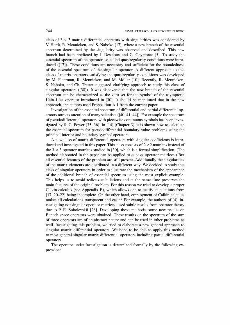
and

Y (y) =

0 0

0x2

m− µx2+ b2(x, µ)

ρ

x2 − β2

x2(m−µx2)

− ρ(0)

m(0)a(µ)

. (48)

Let us remind the reader that everywhere in the paper x is considered as a functionof the variable y, x = e|y|, where we have taken into account the even continuationof all parameters of the matrix for negative values of y. The matrices Q, Y (y) andP(p) satisfy the conditions of Proposition A.1. In addition, the matrix functionsY (y) and P(p) are continuous on the real line and have zero limits at infinity.All matrix functions are depending on the parameter µ. Therefore the essentialspectrum of the resolvent operator M(µ) is given by (72)

σess(M(µ)) = σess(Q + P) ∪ σess(Q + Y).

To calculate the essential spectra of the operators Q + P and Q + Y we use thefact that the determinants of the corresponding matrices Q+ P(p) and Q+ Y (y)are equal to zero identically. It follows that one of the two eigenvalues of the eachmatrix is identically zero. Therefore the essential spectra of the operators coincideswith the range of the second (nontrivial) eigenvalues when y resp.p runs over thewhole real axis. This simple fact is a result of straightforward calculations. Thenontrivial eigenvalues coincide with the traces of the corresponding 2× 2 matricesQ+ P(p) and Q+ Y (y). The trace of the matrix M(µ) is given by

Tr (M(µ)) = Tr (Y (y))+ Tr (P (p))− Tr (Q)

= 1

a(µ)

1

p2 + c(µ) +x2

m− µx2+

+ b2(0, µ)

a(µ)

1/4 − c(µ)p2 + c(µ) + b2(x, µ)

ρ

x2 − β2

x2(m−µx2)

.

The last expression can be factorized into the sum of three factors

Tr(M(µ)) = ϕ(x(y))+ ψ(p)− Tr(Q),

TrQ = ρ(0)

m(0)a(µ),

where the functions ϕ(x(y)) and ψ(p) tend to zero as y resp.p tend to ∞. Thefactorization is unique and obvious

ϕ(x) = x2

m− µx2+ b2(x, µ)

ρ

x2 − β2

x2(m−µx2)

;

ψ(p)= 1

a(µ)

1

p2 + c(µ) +b2(0, µ)

a(µ)

1/4 − c(µ)p2 + c(µ) + ρ(0)

m(0)a(µ).

(49)


Proposition A.1 implies that the essential of the resolvent operator is given by

σess(M(µ)) = (Range(ϕ(x)) ∪ Range(ψ(x))+ ϕ(0)). (50)

Straightforward calculations imply

σess(L) = Rangex∈[0,1]

{m− β2

ρ

x2

}∪[

l0

4 + ρ(0)m(0)

,l0ρ(0)m(0)

], (51)

where l0 is given by (40). The parameter µ disappears eventually as one can expect.This parameter is pure axillary.

We conclude that the essential spectrum of L consists of two parts havingdifferent origin. The so-called regularity spectrum ([30])

Rangex∈[0,1]

{m− β2

ρ

x2

}

is determined by all coefficients of the operator matrix on the whole interval [0, 1].This part of the spectrum coincides with the limit of the essential spectra of thetruncated operators L(ε)

Rangex∈[0,1]

{m− β2

ρ

x2

}=⋃ε>0

σess(L(ε)).

On the contrary the singularity spectrum[l0

4 + ρ(0)m(0)

,l0ρ(0)m(0)

]

is due to the singularity of the operator matrix at the origin and depends on thebehavior of the matrix coefficients at the origin only. This part of the essentialspectrum is absent for all truncated operators L(ε) and cannot be obtained by thelimit procedure ε → 0. This fact explains the name singularity spectrum givenin [30]. The appearance of this interval of the essential spectrum generated bythe singularity was predicted by J. Descloux and G. Geymonat. Note that the endpoint l0/(ρ(0)/m(0)) of the singularity spectrum always belongs to the interval ofregularity spectrum, since

limx→0

m− β2

ρ

x2= l0

ρ(0)m(0)

.

Remark. Let us remind that the essential spectrum has been calculated providedm(0) = 0 and the quasiregularity conditions are satisfied. If m(0) = 0, the qua-siregularity conditions imply that β(0) = 0 and hence m′(0) = 0. No singularity


appears in the coefficients of the matrix L given by (2). Therefore the operator isregular and its essential spectrum equals to

Rangex∈[0,1]

{m− β2

ρ

x2

}(4).

No singularity spectrum appears in this case.There is another way to describe the singularity spectrum using the roots of the

symbol of the asymptotic Hain–Lüst operator, observed first for a different matrixdifferential operator in [30].

LEMMA 9.1. The singularity spectrum[l0

4 + ρ(0)m(0)

,l0ρ(0)m(0)

]

of the operator L coincides with the set of singular points (roots) of the symbol ofthe asymptotic Hain–Lüst operator

. = {µ ∈ R | ∃p ∈ R ∪ {∞} : a(µ)(p2 + c(µ)) = 0}.Proof. The set of singular points of the symbol a(µ)(p2 + c(µ)) coincides with

the set

. = {µ ∈ R | c(µ) � 0}.Formula (40) implies

. ={µ ∈ R | 0 �

l0 − µ ρ(0)m(0)

µ� 4

}

=[

l0

4 + ρ(0)m(0)

,l0ρ(0)m(0)

].

Note that p = ∞ formally corresponds to right endpoint of the last interval. Thelemma is proven. ✷

In our opinion this connection between the singular set of the symbol of theasymptotic Hain–Lüst operator and the singularity spectrum has general character.Studies in this direction will be continued in one of our forthcoming publications.

Remark. We would like to mention that the regularity spectrum

Rangex∈[0,1]

{m− β2

ρ

x2

}under quasiregularity conditions can be calculated using just the symbol of theHain–Lüst operator. Really trivial calculations show that the regularity spectrumcoincides with the set of real µ for which the principle coefficient of the Hain–Lüstoperator degenerates, i.e. equals zero. Roughly speaking this idea has been utilizedby physicists K. Hain and R. Lüst ([16]) (see also [12]).


10. Semiboundedness of the Operator

In many applications to physics semibounded operators play very important role.Semiboundedness of the considered operator is related to the quasiregularity con-ditions.

THEOREM 10.1. Suppose that the real valued functions q, β, ρ,m satisfy thefollowing conditions:

q ∈ L∞[0, 1], β,m, ρ ∈ C2[0, 1], ρ � c0 > 0. (52)

Then the symmetric operator Lmin corresponding to the operator matrix (2) issemibounded if and only if one of the following three conditions is satisfied

(1) (m− β2/ρ)|x=0 > 0,(2) (m− β2/ρ)|x=0 = 0 and (m− β2/ρ)′|x=0 > 0,(3) (m− β2/ρ)|x=0 = 0 and (m− β2/ρ)′|x=0 = 0 (quasiregularity conditions).

COROLLARY 10.1. Under assumptions of Theorem 10.1 the operator Lmin ad-mits self-adjoint extensions. Every such extension L is a semibounded operator ifand only if one of the conditions (1)–(3) is satisfied.

Proof. Since the coefficients of the matrix L are real valued functions, the defi-ciency indices of Lmin are equal. On the other hand the equation for the deficiencyelement is a system of ordinary differential equations. Therefore the set of solutionshas finite dimension. Hence the operator Lmin always has finite equal deficiencyindices and admits self-adjoint extensions. Theorem 10.1 implies that every suchextension is semibounded if and only if one of the three conditions is satisfied(see [3]). ✷

Proof of Theorem 10.1. Without loss of generality one can suppose that q = 0,since the operator corresponding to the matrix

(q 00 0

)is bounded in H and cannot

change the semiboundedness of the whole operator Lmin.The theorem will be proven by estimating the quadratic form of Lmin defined on

the domain C∞0 [0, 1] ⊕ C∞

0 [0, 1] by the following operator matrix

L =

− d

dxρ

d

dx

d

dx

β

x

−βx

d

dx

m

x2

. (53)

The quadratic form of this operator is

〈LminU,U 〉 = 〈ρu′1, u′1〉 −⟨β

xu2, u

′1

⟩−⟨β

xu′1, u2

⟩+⟨m

x2u2, u2

⟩


=⟨

1 − β√ρ

− β√ρ

m

√ρu′1u2

x

,

√ρu′1u2

x

⟩ . (54)

Considering functions with zero second component U = (u1, 0) we concludethat the operator Lmin is not bounded from above, since the quadratic form coin-cides with the quadratic form of the operator −(d/dx)ρd/dx in this case. Thereforethe operator Lmin is semibounded if and only if it is bounded from below. To getthe second necessary condition for the semiboundedness of the operator considerthe set of functions with zero first component U = (0, u2). The quadratic form isthen given by

〈LminU,U 〉 =⟨m

x2u2, u2

⟩.

Hence the operator Lmin is semibounded only if

m(0) > 0 or m(0) = 0 and m′(0) � 0. (55)

Case A. Suppose that the determinant of the matrix

det

1 − β√ρ

− β√ρ

m

= m− β2

ρ

is negative at point zero (and therefore in a neighborhood of this point as well)

m(0)− β(0)2

ρ(0)< 0. (56)

It follows that the matrix has precisely one negative eigenvalue λ(x) < 0 for smallenough values of x. Let us denote by (α, γ ) the corresponding normalized realeigenvector depending continuously on x in a neighborhood of the origin.

Suppose that α(0) = 0. Then the first equation for the eigenvector implies thatβ(0) = 0 and therefore m(0) < 0 due to (56). This contradicts (55) and thereforeα(0) = 0 in a certain neighborhood of the origin due to the continuity of α.

Consider arbitrary real function h ∈ C∞0 [0, 1] such that the derivative of h

is equal to 1 in the interval (1/4, 1/2) and the family of scaled functions hε =εh(x/ε). The corresponding family of vector functions Uε = (hε,

γ

α

√ρxhε ′) is

well-defined for sufficiently small ε. Since

〈LminUε,Uε〉 =

∫ ε

0

λ(x)ρ

α2hε

′2 dx,


and

‖Uε‖2 =∫ ε

0

(hε2 + γ 2ρ

α2x2hε ′2

)dx,

the quotient 〈LU,U 〉/‖ U ‖2 tends to −∞ as ε → 0. Hence the operator Lmin isnot semibounded in this case.

Case B. Suppose that

m(0)− β(0)2

ρ(0)> 0.

The operator L is semibounded in this case. Indeed the quadratic form can bedecomposed as follows

〈LminU,U 〉 =⟨

1 − β(0)√ρ(0)

− β(0)√ρ(0)

m(0)

√ρu′1

u2

x

,

√ρu′1

u2

x

⟩+

+⟨

0β(0)√ρ(0)

− β√ρ

β(0)√ρ(0)

− β√ρ

m−m(0)

√ρu′1

u2

x

,

√ρu′1

u2

x

⟩.

The first term is positive and can be estimated from below by

const(‖u′1‖2 + ‖u2‖2)

due to the assumption. The second term is subordinated to the first one∣∣∣∣∣∣∣∣∣⟨

0β(0)√ρ(0)

− β√ρ

β(0)√ρ(0)

− β√ρ

m−m(0)

√ρu′1

u2

x

,

√ρu′1

u2

x

⟩∣∣∣∣∣∣∣∣∣

� const∫ 1

0

(xu′1

2 + u22

x

)dx

� const ε∫ ε

0

(ρu′1

2 + u22

x2

)dx + const

∫ 1

ε

(u′1

2 + u22

x2

)dx.

The relative bound const ε can be chosen less than 1 and the second term isbounded for any ε > 0.

Case C. Suppose that

m(0)− β(0)2

ρ(0)= 0 and

d

dx

(m− β2

ρ

)|x=0 < 0.


The quadratic form can be decomposed as

〈LminU,U 〉 =⟨(

1 −β/√ρ−β/√ρ β2/ρ

)√ρu′1u2

x

,

√ρu′1u2

x

⟩+

+⟨(

0 0

0 m− β2/ρ

)

√ρu′1u2

x

,

√ρu′1u2

x

⟩.

Consider the vector function

V ε =(∫ x

0

β(t)

ρ(t)hε

′(t) dt, xhε ′(x)

),

where the scalar hε has been introduced investigating Case A. Calculating the thequadratic form

〈LminVε, V ε〉 =

⟨(m− β2

ρ

)hε

′, hε

′⟩

and estimating the norm

‖V ε‖2 =∫ 1

0

[x2hε

′2 +(∫ x

0

β

ρhε

′ dt)2]

dx

�∫ 1

0[x2hε

′2 + const hε2] dx.

Since (m− (β2/ρ))′|x=0 < 0, the quotient

〈LU,U 〉‖U‖2

tends to −∞ as ε → 0. The operator is not semibounded in this case.

Case D. Suppose that(m− β2

ρ

)|x=0 = 0 and

(m− β2

ρ

)′|x=0 � 0. (57)

The operator Lmin is semibounded in this case due to the following estimate⟨(0 0

0 m− β2/ρ

)

√ρu′1u2

x

,

√ρu′1u2

x

⟩

=∫ 1

0

m− β2

ρ

x2|u2|2 dx � const‖u2‖2,


which is valid since the function (m− (β2/ρ))/x2 from below.The Cases A–D cover all the possibilities. The Theorem is proven. ✷

Appendix A. On the Essential Spectrum of the Triple Sum of Operators inBanach Space

The following simple lemma will be used to calculate the essential spectrum of theseparable sum of pseudodifferential operators. It allows one to pass to the limit informula (58) below when the point λ reaches the discrete spectrum.

LEMMA A.1. Let T,Y,P be bounded operators acting in a Banach space X.Suppose that a certain dotted neighborhood of λ = 0 does not belong to thespectrum of the operator T and the point λ = 0 is not in the essential spectrum ofthe operator T. � Suppose in addition that

Y(T − λ)−1P ∈ S∞ (58)

is a compact operator in the dotted neighborhood. Let RT be the parametrix of theoperator T ([13])

RTT =TRT = I. (59)

Then the operator YRTP is compact

YRTP ∈ S∞. (60)

Proof. The following calculations prove the lemma

YRTP := Y(T − λ)−1(T − λ)RTP= Y(T − λ)−1(I − λRT)P= −λY(T − λ)−1RTP= −λYRT(I − λRT)

−1RTP= 0,

(61)

where the second equality from the end is valid for all λ, 0 < |λ| < 1/‖RT‖ notfrom the spectrum of the operator T

(T − λ)R = I − λR ⇒ (T − λ)−1 =R(I − λR)−1.

The lemma is proven. ✷� These conditions imply that the point λ = 0 is a finite type eigenvalue of T ([13]) or does not

belong to the spectrum of T at all. In the last case the proof of the lemma is trivial.


THEOREM A.1. Let M be the operator sum of three bounded operators Q, Y andP acting in a certain Banach space

M = Q + Y + P, (62)

such that the complement in C of the essential spectrum of the operator Q is con-nected. Suppose that the following two operators are compact for any λ from theregular set of Q

P1

Q − λY ∈ S∞; Y1

Q − λP ∈ S∞. (63)

Then the essential spectrum of the operator M can be calculated as follows

σess(M) \ σess(Q) = [σess(Q + Y) ∪ σess(Q + P)] \ σess(Q). (64)

Proof. It has been proven in [13] (Corollary 8.5, page 204) that if the comple-ment in C of the essential spectrum of a certain bounded operator is connected,then any number λ from the spectrum of the operator, but not from the essentialspectrum is a finite type eigenvalue ([13]), i.e. the pole of the resolvent with fi-nite rank Laurent coefficients with negative indices. Lemma A.1 implies that theoperators

YRQ(λ)P, PRQ(λ)Y (65)

are compact operators, where RQ(λ) is one of the parametrix of the operator Q atpoint λ

(Q − λ)RQ(λ) =RQ(λ)(Q − λ) = I. (66)

Then the following equalities can be proven

(Q + Y − λ)RQ(λ)(Q + P − λ) =Q + Y + P − λ;(Q + P − λ)RQ(λ)(Q + Y − λ) =Q + Y + P − λ. (67)

Let us prove the first equality only, since the prove of the second equality is similar.Formulas (65) imply that

(Q + Y − λ)RQ(λ)(Q + P − λ)= (I + YRQ(λ))(Q + P − λ)=Q − λ+ YRQ(λ)(Q − λ)+ P + YRQ(λ)P

=Q + Y + P − λ.We are going to prove now formula (64) for the essential spectra of the operators

M, Q, Y, and P following the idea of [17], where a similar fact has been proven tothe sum of two operators. Let us prove the following inclusion first

σess(M) \ σess(Q) ⊂ [σess(Q + Y) ∪ σess(Q + P)] \ σess(Q). (68)


Suppose that λ does not belong to the essential spectra of the operators Q, Q + Y,and Q + P, then the operators

Q + Y − λ, RQ(λ), Q + P − λare Fredholm operators as a product of three Fredholm operators. Then formulas(67) imply that the operator

Q + Y + P − λis a Fredholm operator. Hence the point λ does not belong to the essential spectrumof the operator Q + Y + P.

In the second step let us prove the inclusion

σess(M) \ σess(Q) ⊃ [σess(Q + Y) ∪ σess(Q + P)] \ σess(Q). (69)

Suppose that λ does not belong to the essential spectra of the operators M and Q,i.e. that the operators M − λ and Q − λ are Fredholm operators. We are going touse Proposition 8.2 from [17] (see also [13]) stating that if the operators A andB are two bounded operators acting in a certain Banach space and the operatorsAB and BA are Fredholm operators, then the operators A and B are also Fredholmoperators. Formulas (67) imply that the operators

RQ(λ)(Q + Y − λ)RQ(λ)(Q + P − λ)and

RQ(λ)(Q + P − λ)RQ(λ)(Q + Y − λ)are Fredholm operators. Then the proposition implies that the operators RQ(λ)(Q+Y − λ) and RQ(λ)(Q + P − λ) are Fredholm operators. It follows from (66) thatthe operators

Q + Y − λ = (Q − λ)RQ(λ)(Q + Y − λ)and

Q + P − λ = (Q − λ)RQ(λ)(Q + P − λ)are Fredholm operators. It follows that λ does not belong to the essential spectra ofthe operators Q + Y and Q + P. Inclusion (69) is proven.

Formulas (68) and (69) imply (64). The Theorem is proven. ✷Remark. It is possible to get read of the condition that the complement in C of

the essential spectrum the operator Q is connected. Then it is necessary to supposethat the operators YRQ(λ)P, PRQ(λ)Y are compact for any λ outside the essentialspectrum of Q. It is possible to construct three operators Q,P,Y satisfying allconditions of the theorem except the connectivity of C \ σess(Q) but not satisfyingformula (64). This counterexample can be prepared using bilateral shift in theHilbert space X = ?2

Z(?2N,H ⊕ H), where H is a certain infinite dimensional

axillary Hilbert space.


PROPOSITION A.1. Let M be any n × n matrix separable pseudodifferentialoperator generated in the Hilbert space L2(R,Cn) by the symbol

M(y, p) = Q+ Y (y)+ P(p), p = 1

i

d

dy, (70)

where Q is a constant diagonalizable matrix with simple spectrum, and the matrixfunctions Y (y) and P(p) are essentially bounded and satisfy the following twoasymptotic conditions

limx→∞Y (y) = 0 lim

p→∞P(p) = 0. (71)

Then the essential spectrum of the operator M is given by

σess(M) = σess(Q + P) ∪ σess(Q + Y). (72)

Proof. The essential spectra of both operators Q + Y and Q + P contain theessential spectrum of Q

σess(Q) = σ (Q),

where σ (Q) is the spectrum of the matrix Q. To prove this fact one can use pertur-bation theory and the fact that the matrices Y (y), y → ∞ and P(p), p → ∞ areasymptotically small ([24]).

Theorem A.1 implies that

σess(Q + Y + P) \ {0} ⊃⋃n

σess(PN(Q + Y)PN) \ {0} ⊃ σ (Q) \ {0},

(using A = Q + Y, B = P ). It follows that

σess(M) \ {0} = (σess (Q + P) ∪ σess (Q + Y)) \ {0}. (73)

We are going to remove the set {0} from the last formula.Applying the same analysis for the operator M − εI we obtain that

σess(M − εI) \ {0} = (σess (Q − εI + P) ∪ σess (Q − εI + Y)) \ {0}. (74)

This implies that

σess(M(y, p)) \ {ε} = (σess(Q + P) ∪ σess(Q + Y)) \ {ε},for arbitrary real ε and hence

σess(M) = (σess(Q + P) ∪ σess(Q + Y)). (75)

The proposition is proven. ✷In the special case case n = 1 and when the symbols Y (y) and P(p) are

piecewise continuous the last proposition can be derived from Theorem 3 in [35](see also [36]). The advantage of our approach is its transparency compared withthe technique of C∗ algebras used in [35].


Remark. The condition concerning the simplicity of the spectrum of matrixQ can be removed in the special case where all matrices Q,Y (y), and P(p) areHermitian.

Proof. Consider the family of small Hermitian perturbations Qε, ε > 0 of thematrix Q such that

‖ Qε −Q ‖� ε

and the spectrum of Qε is simple. Such matrix Qε satisfy the conditions of thetheorem and hence

σess(Qε + Y + P) = σess(Qε + P) ∪ σess(Qε + Y). (76)

Let us denote by Fδ the δ-neighborhood of any set F ⊂ R

Fδ := {x ∈ R : dist(x, F ) � δ}.LetA and B be two bounded self-adjoint operators acting in a certain Hilbert space.Then the essential spectra of the operators A and A+B are related by the followingformula ([3])

σess(A + B) ⊂ (σess(A))‖B‖.

From (76) we immediately obtain that

σess(Q + Y + P(p)) ⊂ [σess(Qε + Y) ∪ σess(Qε + P)]2ε;σess(Q + Y) ∪ σess(Q + P) ⊂ [σess(Qε + Y + P)]2ε.

Since the essential spectra are closed sets and ε is arbitrary small, we conclude that

σess(Qε + Y + P) = σess(Q + Y) ∪ σess(Q + P). (77)

This completes the proof. ✷

Appendix B. Elementary Lemmas on Calkin Calculus

The following lemmas are necessary for the transformation of the resolvent.

LEMMA B.1. Let the real valued function f (y) be positive bounded and sepa-rated from zero

0 < c � f (y) � C (78)

for some c, C ∈ R+. Let the function g(y) be bounded and the operator

L ≡ pf (y)p + g(y) (79)


be self-adjoint and invertible in L2(R). Suppose that the operator pL−1p bebounded. � Then for any bounded function h(y) such that limy→∞ h(y) = 0 thefollowing equality holds in Calkin algebra

pL−1ph = h

f. (80)

Comment 1. The role of the function h is to regularize the equality which doesnot hold in Calkin algebra pL−1 = 1/f . Therefore the regularizing function h can-not be cancelled in (80). To construct a counter example let us first consider similarproblem on the whole axis for which all calculations are trivial. Let the functionsf and g be constant functions f = 1, g = 1. Then the operator

pL−1p − 1 = p(p2 + 1)−1p − 1 = − 1

p2 + 1

obviously is not compact, since it is a multiplication operator in the Fourier repre-sentation.

Comment 2. In [4] similar result has been obtained in the regular case. Herean abstract proof of a generalization of the result is presented. We hope that thealgebraic character of the proof will enable us to generalize these results to a widerclasses of PDO and CDO. The advantage of our approach is that no informationconcerning the Green’s function is used.

Proof. Consider first the case where the function h(y) is a C∞(R) function.We need this condition in order to avoid to consider the closure of bounded op-erators considered below. All these operators are well defined by their differentialexpressions on W 1

2 (R).The following identity holds (at least in W 1

2 (R))

((p + i)L−1(p − i))(

1

p − i L1

p + i)= I.

Multiplying the latter equality by the operator of multiplication by decreasingfunction h one can get the operator equality valid on W 1

2 (R)

((p + i)L−1(p − i)) 1

p − i (pfp)1

p+ i h+

+ ((p + i)L−1(p − i)) 1

p − i g1

p + i h = h.

The second term in left-hand side is a compact operator as the multiplication ofthe bounded operator (p + i)L−1(p − i)(1/(p − i))g and the compact operator

� The latter condition could follow from the previous conditions for sufficiently smoothfunction f .


(1/(p + i))h (since the functions 1/(p + i) and h are decreasing function of pand y respectively). Hence the following equality holds in Calkin algebra

((p + i)L−1(p − i)) 1

p − i (pfp)1

p+ i h =h.

Similarly taking into account that

p1

p + i h =(

1 − i

p + i)h =h

we get the following equality

((p + i)L−1(p − i)) 1

p − i pf h =h.

Multiplying by f −1 the latter equality, one gets

(p + i)L−1(p − i) 1

p − i ph =h

f,

using the fact the function f is boundedly invertible. Multiplying the latter equalityby factor

p

p + i = 1 − i

p + ifrom the left one gets in Calkin algebra

h

f= p

p + i (p + i)L−1(p − i) p

p − i hp

p − i = pL−1ph.

Let us consider the case of decreasing bounded but otherwise arbitrary func-tion h. Every such function can be estimated from above by a certain positivedecreasing to zero C∞(R) function h, |h(y)| � h. We have already proven theLemma for the function h

h

f= p

p + i (p + i)L−1(p − i) p

p − i hp

p − i = pL−1ph.

Of cause the multiplication by the contraction operator of multiplication by thebounded function h/h preserves the equality in Calkin algebra. Finally one gets(80) for arbitrary h satisfying the conditions of the Lemma. ✷

The following lemma is well-known. (It is a special case of problems treatedsystematically in [19].)

LEMMA B.2. Let the following conditions be satisfied


(i) f � c > 0,(ii) f, g ∈ C1(R),

(iii) (pfp + g)|W 22 (R)

is invertible, then the operator (p + i)(pfp + g)−1(p − i)defined originally on the dense set W 1

2 (R) is bounded in L2(R).

COROLLARY. Under conditions of the lemma the operator

p(pfp + g)−1p|W 12 (R)

is also bounded, since the operator p/(p ± i) is a contraction.

Remark. Condition (iv) can be substituted by a stronger condition (iv′) the realvalued function g is positive definite g(x) � c0 > 0. Really conditions (i), (ii), (iii)(iv′) imply (iv), since the estimate

〈(pfp + g)u, u〉 = 〈fpu, pu〉 + 〈gu, u〉 � c0‖pu‖2 + c0‖u‖2

implies that the operator (pfp + g)|W 22 (R)

has bounded inverse.

LEMMA B.3. Suppose that conditions (i)–(iii) of Lemma B.2 be satisfied. Let inaddition the limits

limy→∞f (y), lim

y→∞ g(y),

be finite. Then the difference between the inverse Hain–Lüst and asymptotic Hain–Lüst operators is a compact operator, moreover

(p + i)[T −1(µ)− T −1as (µ)] ∈ S∞;

[T −1(µ)− T −1as (µ)](p − i) ∈ S∞. (81)

Proof. Consider the following chain of equalities

(p + i)[T −1(µ)− T −1as (µ)] ∈ S∞

= (p + i)T −1(µ){Tas(µ)− T (µ)]T −1(µ)

= (p + i)T −1(µ)(pf p + g)T −1(µ)

= (p + i)T −1(µ)(p − i)(p − i)−1(pf p + g)T −1(µ),

where

f = f − limy→∞ f (y) ∈ C

1(R),

g = g − limy→∞ g(y) ∈ L

∞(R) ∩ C1(R),

limy→∞ f (y) = lim

y→∞ g(y) = 0.


The operator (p+ i)T −1(µ)(p− i) is bounded and the operator (p− i)−1(pf p+g)T −1(µ) is compact operators, since the operators

(p − i)−1g and f pT −1(µ)

are compact. (Here we use the fact that any pseudodifferential operator deter-mined by the symbol ϕ(x)ψ(p) is compact if ϕ,ψ ∈ C(R) and limx→∞ ϕ(x) =0, limp→∞ ϕ(p) = 0.) The lemma is proven. ✷LEMMA B.4. Let conditions (i)-(iii) of Lemma B.2 be satisfied. Suppose in ad-dition that the continuous functions α, γ ∈ C(R) are continuous and have finitelimits at infinity. Then the following equality holds in Calkin algebra

(αp + γ )T −1(µ) = (α(∞)p + γ (∞))T −1as (µ). (82)

Proof. Lemma B.3 implies that

(αp + γ )T −1(µ)

= (αp + γ )T −1as (µ)

= (α(∞)p + γ (∞))T −1as (µ)+ ((α − α(∞))p + γ − γ (∞))T −1

as (µ)

= (α(∞)p + γ (∞))T −1as (µ)+ (α − α(∞))pT −1

as (µ)+ (γ − γ (∞))T −1as (µ)

= (α(∞)p + γ (∞))T −1as (µ).

The lemma is proven. ✷Remark. All lemmas proven in this appendix for the operators acting in L2(R)

are in fact valid for the corresponding operators restricted to L2(R+). To make theoperators self-adjoint in L2(R+) one needs to introduce some additional symmetricboundary condition at the origin, for example the Dirichlet boundary condition dis-cussed in the paper. Let us mention here the necessary modifications of Lemma B.1only. The other lemmas can be treated in the same way. Let L be a self-adjoint op-erator in L2(R+) determined by (79) and certain boundary condition at the origin.Consider the extension of L to the operator acting inL2(R) determined by the sameexpression, where the functions f (y) and g(y) are continued for negative valuesof y as even functions. Then equality (80) holds in Calkin algebra for the extendedoperator. Taking into account that the resolvent of the extended operator differsfrom the orthogonal sum of two copies of the resolvents of the initial operator takenon the positive and negative semiaxes separately by a finite rank operator. (Note thatthe functions from the domain of both operators satisfy proper separating boundaryconditions at the origin.) We have used here the Glazman splitting method ([3]).As a result, we obtain the necessary equality for the operators in L2(R+).

Acknowledgements

We would like to thank the referee for valuable remarks which allowed us toimprove the original manuscript.


The work of the authors was supported by the Royal Swedish Academy ofSciences.

References

1. Adam, J. A.: Critical layer singularities and complex eigenvalues in some differential equationsof mathematical physics, Phys. Rep. 142 (1986), 263–356.

2. Adamyan, V., Langer, H., Mennicken, R. and Saurer, J.: Spectral components of self-adjointblock operator matrices with unbounded entries, Math. Nachr. 178 (1996), 43–80.

3. Akhiezer, N. I. and Glazman, I. M.: Theory of Linear Operators in Hilbert Space, Pitman,Boston, 1981.

4. Atkinson, F. V., Langer, H., Mennicken, R. and Shkalikov, A.: The essential spectrum of somematrix operators, Math. Nachr. 167 (1994), 5–20.

5. Descloux, J. and Geymonat, G.: Sur le spectre essentiel d’un operateur relatif á la stabilité d’unplasma en géometrie toroidal, C.R. Acad. Sci. Paris 290 (1980), 795–797.

6. Everitt, W. N. and Bennewitz, C.: Some remarks of the Titchmarsch–Weyl m-coefficient, In:Tribute to Åke Pleijel, Univ. of Uppsala, 1980.

7. Everitt, W. N. and Markus, L.: Boundary Value Problems and Symplectic Algebra for OrdinaryDifferential and Quasi-differential Operators, Amer. Math. Soc., Providence, RI, 1999.

8. Faierman, M., Lifschitz, A., Mennicken, R. and Möller, M.: On the essential spectrum of adifferentially rotating star, ZAMM Z. Angew. Math. Mech. 79 (1999), 739–755.

9. Faierman, M., Mennicken, R. and Möller, M.: The essential spectrum of a system of singularordinary differential operators of mixed order. I. The general problem and an almost regularcase, Math. Nachr. 208 (1999), 101–115.

10. Faierman, M., Mennicken, R. and Möller, M.: The essential spectrum of a system of singularordinary differential operators of mixed order. II. The generalization of Kako’s problem, Math.Nachr. 209 (2000), 55–81.

11. Faierman, M. and Möller, M.: On the essential spectrum of a differentially rotating star in theaxisymmetric case, Proc. Royal Soc. Edinburgh A, 130 (2000), 1–23.

12. Goedbloed, J. P.: Lecture notes on ideal magnetohydrodynamics, In: Rijnhiuzen Report, Form-Instituut voor Plasmafysica, Nieuwegein, 1983, 83–145.

13. Gohberg, I., Goldberg, S. and Kaashoek, M.: Classes of Linear Operators, vol. 1, Birkhäuser,Basel, 1990.

14. Grubb, G.: Functional Calculus of Pseudodifferential Boundary Problems, 2nd edn,Birkhäuser, Basel, 1986.

15. Grubb, G. and Geymonat, G.: The essential spectrum of elliptic systems of mixed order, Math.Anal. 227 (1977), 247–276.

16. Hain, K. and Lüst, R.: Zur Stabilität zylindersymmetrischer Plasmakonfigurationen mitVolumenströmmen, Z. Naturforsch. A 13 (1958), 936–940.

17. Hardt, V., Mennicken, R. and Naboko, S.: System of singular differential operators of mixedorder and applications to 1-dimensional MHD problems, Math. Nachr. 205 (1999), 19–68.

18. Hartman, P.: Ordinary Differential Equations, John Wiley, New York, 1964.19. Hörmander, L.: The Analysis of Linear Partial Differential Operators, vols I–IV, 2nd edn,

Springer-Verlag, Berlin, 1994.20. Kako, T.: On the essential spectrum of MHD plasma in toroidal region, Proc. Japan Acad. Ser.

A Math. Sci. 60 (1984), 53–56.21. Kako, T.: On the absolutely continuous spectrum of MHD plasma confined in the flat torus,

Math. Methods Appl. Sci. 7 (1985), 432–442.22. Kako, T.: Essential spectrum of linearized operator for MHD plasma in cylindrical region,

Z. Angew. Math. Phys. 38 (1987), 433–449.


23. Kako, T. and Descloux, J.: Spectral approximation for the linearized MHD operator incylindrical region, Japan J. Indust. Appl. Math. 8 (1991), 221–244.

24. Kato, T.: Perturbation Theory for Linear Operators, 2nd edn, Springer, Berlin, 1976.25. Konstantinov, A. and Mennicken, R.: On the Friedrichs extension of some block operator

matrices, Integral Equations Operator Theory 42 (2002), 472–481.26. Krasnosel’skii, M. A., Zabreiko, P. P., Pustylnik, E. I. and Sobolevskii, P. E.: Integral Operators

in Spaces of Summable Functions, Noordhoff Publishing, Leiden, 1976.27. Kurasov, P.: On the Coulomb potential in one dimension, J. Phys. A 29 (1996), 1767–1771;

Response to ‘Comment on “On the Coulomb potential in one dimension”,’ J. Phys. A 30 (1997),5579–5581.

28. Langer, H. and Möller, M.: The essential spectrum of a non-elliptic boundary value problem,Math. Nachr. 178 (1996), 233–248.

29. Lifchitz, A. E.: Magnetohydrodynamics and Spectral Theory, Kluwer Acad. Publ., Dordrecht,1989.

30. Mennicken, R., Naboko, S. and Tretter, Ch.: Essential spectrum of a system of singulardifferential operators, to appear in Proc. Amer. Math. Soc.

31. Möller, M.: On the essential spectrum of a class of operators in Hilbert space, Math. Nachr. 194(1998), 185–196.

32. Naboko, S.: Nontangential boundary values of operator-valued R-functions in a half-plane,St. Petersburg (Leningrad) Math. J. 1 (1990), 1255–1278.

33. Naimark, M. A.: Linear Differential Operators, Ungar, New York, 1968.34. Olver, F. W.: Introduction to Asymptotic and Special Functions, Academic Press, New York,

1974.35. Power, S. C.: Essential spectra of piecewise continuous Fourier integral operators, Proc. Roy.

Irish. Acad. 81 (1981), 1–7.36. Poer, S. C.: Fredholm theory of piecewise continuous Fourier integral operators on Hilbert

space, J. Operator Theory 7 (1982), 51–60.37. Raikov, G. D.: The spectrum of a linear magnetohydrodynamic model with cylindrical

symmetry, Arch. Rational Mech. Anal. 116 (1991), 161–198.38. Rofe-Beketov, F.: Self-adjoint extensions of differentila operators in a space of vector-

functions, Soviet. Math. Doklady 10 (1969), 188–192.39. Rofe-Beketov, F. and Kholkin, A.: Spectral Analysis of Differential Operators. Relation of the

Spectral and Oscillatory Properties, Mariupol, 2001.40. Schechter, M.: On the essential spectrum of an arbitrary operator. I, J. Math. Anal. Appl. 13

(1966), 205–215.41. Schechter, M.: Spectra of Partial Differential Operators, 2nd edn, North-Holland, Amsterdam,

1986.42. Reed, M. and Simon, B.: Methods of Modern Mathematical Physics, 2nd edn, vols I–IV.

Academic Press, New York, 1984.43. de Snoo, H.: Regular Sturm–Liouville problems whose coefficients depend rationally on the

eigenvalue parameter, Math. Nachr. 182 (1996), 99–126.44. Zelenko, L. B. and Rofe-Beketov, F. S.: The limit spectrum of systems of first order differential

equations with slowly changing coefficients (Russian), Differencial’nye Uravnenija 7 (1971),1982–1991 (in Russian).

staff.math.su.sestaff.math.su.se/kurasov/pdfarchiv/naboko12-kluwer.pdf · mathematical physics,...

Documents