stable boundary layer modeling at the met office

© Crown copyright Met Office

Stable boundary layer modeling at the Met Office

Adrian Lockwith contributions from many other Met Office staff


Outline

• Current operational configurations and performance

• “Recent” changes

• Stable boundary layers in complex terrain (COLPEX)

• Fog

• Summary


Current operational configurations

© Crown copyright Met Office© Crown copyright Met Office

The operational forecast modelsNWP horizontal grid lengths, lid:

• Global NWP: ~25 km, 80km

• Global seasonal: ~135km, 80km

• [N.Atlantic/Europe: 12 km, 80km]

• UK: 1.5km, 40km


Operational configurations

• Current global climate-seasonal configuration = GA3.0

• Documented in Walters et al (Geoscientific Model Development, 2011)

• PBL scheme = non-local K-profile + local Ri for SBLs

• Massflux scheme for convection, PC2 prognostic cloud scheme, etc

• N96 (~135km) and L85 (80km lid, 9 levels below 1km)

• Current global NWP = GA3.1 = GA3.0 except:

• Enhanced SBL mixing: “long tail” stability functions over land (instead of “Mes”), λM doubled in PBL, no reduction of λ (to 40m) above PBL top

• Single aggregate surface tile (cf 9 tiles)

• N512 (~25km) and L70 (reduced stratospheric resolution)

• UK model (UKV for “variable” grid but mainly 1.5km)

• As GA3.0 but no convection parametrization, Smith fixed pdf cloud scheme, Smagorinsky diffusion in horizontal

• Very nearly the same PBL scheme (eg same stability functions)

• L70_UK (40km lid, 16 levels below 1km)


Operational vertical grids

Current vertical grids (lowest levels for U/T):

Gbl (10m/20m)

UKV (2.5m/5m)

UKV levels thinner, ~70%

L140 (1m/2m)


PBL Tails

• f(Ri) in local scheme (used for SBLs):

• SHARPEST over sea, “Mes tail” over land (except “long tail” in GA3.1)

• “Mes tail” motivated by surface heterogeneity = linear transition between Louis at z=0 and SHARPEST at z=200m

( )Rifdz

duK

2λ=


Why GA3.1 for NWP?• Suppresses (but doesn’t fix) systematic errors of GA3.0

• Single tile gives cooling especially where significant tree fraction

• Reduces North American negative PMSL bias in particular

• Long-tail warms deserts at night (reduce emissivity instead?)


Summer diurnal cycle of biasesfor Europe (global forecasts from 12Z)

• Too warm at night (except deserts), too cold by day

• Sharper tail only gives small (0.1-0.2K) cooling at night

• Too much cloud at night (consistent), too little by day (inconsistent!)

• but cloud cover verification not easy to interpret

Temperature Cloud cover

GA3.0

GA3.1GA3.0+Sharpest

12Z

0Z0Z

12Z


Diurnal cycle of UK clear sky T bias

• Still too warm at night, too cold by day, even when cloud free

• Day:

• Excessive evaporation?

• Too well-mixed?

• Night:

• Excessive turbulent mixing (mes tail)?

• Grid-box mean cf grass?

• Role of ground heat flux in suppressing diurnal cycle?

• Revisit surface roughness (currently z0h=0.1z0m)

• Looks like it ought to be tractable!

• Further analysis of SEB errors needed

Colours denote forecast range


Relevant “recent” changes to PBL scheme


Not so recent!

• Brown et al (2008)

• Non-local momentum transport

• reduces slow daytime wind bias over land

• SHARPEST tails over the sea

• Both improve surface drag and forecast wind direction over the sea

• John Edwards’ decoupled screen T diagnostic

• Frictional heating from turbulent dissipation (~τidui/dz)

• Non-trivial near-surface warming (up to 1K/day)

• Monotonically damping, second-order-accurate, unconditionally-stable implicit solver of Wood et al. (2007)

• Huge reduction of noise in near surface winds/temperatures


UKV (1.5km) valley cooling problemsWinter 2010

• Screen T up to 20K too cold in Scottish valleys

• Goes away if orography smoothed to 12km – not popular!

• Standard is to use Raymond filter that suppresses 2∆ completely, 4∆by 50% and 6∆ hardly at all

• Suggestion that flow decouples over valleys too readily (period actually quite windy)

• Similar problems seen in 12km models with steep 6∆ valleys (~70km across – ie Himalayas)

T1.5m12Z 2nd Feb

Control Control + 12km orography

-20C 0C

Orographic height


Valley cooling

(Std)

(12km)

?

“Nearby”


Subgrid drainage shear

• Initial attempts to related length of tail to orography (eg McCabe and Brown, 2007) had little impact as resolved Ri typically large

• Instead, approximate the wind shear associated with unresolved orographic drainage flows on slopes of α as

• Include this wind shear in the turbulent mixing parametrization, as an enhancement to the standard resolved scale vertical wind shear

• Typical values for N2~1K/100m, α~0.15 and t=30mins givesS

d~ 0.1s-1, or a drainage flow of 2ms-1 at 20m.

• This then implies Ri~0.04 and K~1 m2s-1

( )hd zftNS σα /2=

( ) ( )( )2

22 with

d

dSS

NRiRifSSK+

=+= λ


UKV valley cooling

• Including this representation of shear from unresolved drainage flows in local PBL scheme

• Safely allows use of high res orography (~6km) in 1.5km model

• No subsequent sign in verification of a warm bias in orographicregions

T1.5m at 12Z 2/2/10

Control Control + 12km orography Control+drainage flow


Stable boundary layers in complex terrainFirst results


COLPEX Met Office / NCAS

• Extensively instrumented hills and valleys in Shropshire for ~1year

• Very high resolution (100m) UM simulations

• Provide a database which will aid interpretation of the observations

• Inform choices about the next generation of operational forecast models

• To better understand the mechanisms leading to the formation of cold pools, drainage flows and fog in valleys

• Evaluate the performance of 1.5km operational forecasts and develop improvements:

• Coarse-grain 100m UM to inform parametrization developments

• eg the parametrization of shear from unresolved drainage flows

• surface temperature downscaling


Photos courtesy of Jeremy Price and Dave Bamber, MRU Cardington

2-3km


Upper DuffrynValley site

• 3 main sites

• 30/50m masts with sonics, T, q; radiometers; ground heat flux and temperature; visibility measurements

• doppler lidar

• frequent sondes during 17 IOPs

• ~20 other AWS sites


COLPEX_100 Orography

Colpex_100domain

100m innerdomain

Upper DuffrynSpringhill

Burfield

30km


9th September 2009 IOP

• Initial focus on a clear-sky COLPEX IOP

• Simulation from 15UTC 09 to 15 UTC 13 September 2009

00 UTC 10/09/2009


Potential temperature at 2m, winds at 1m

2009/09/09 1800 UTC 2009/09/09 1900 UTC

10km


2009/09/09 1800 UTC 2009/09/09 1900 UTC2009/09/09 2000 UTC 2009/09/09 2100 UTC



2009/09/09 2200 UTC 2009/09/09 2300 UTC



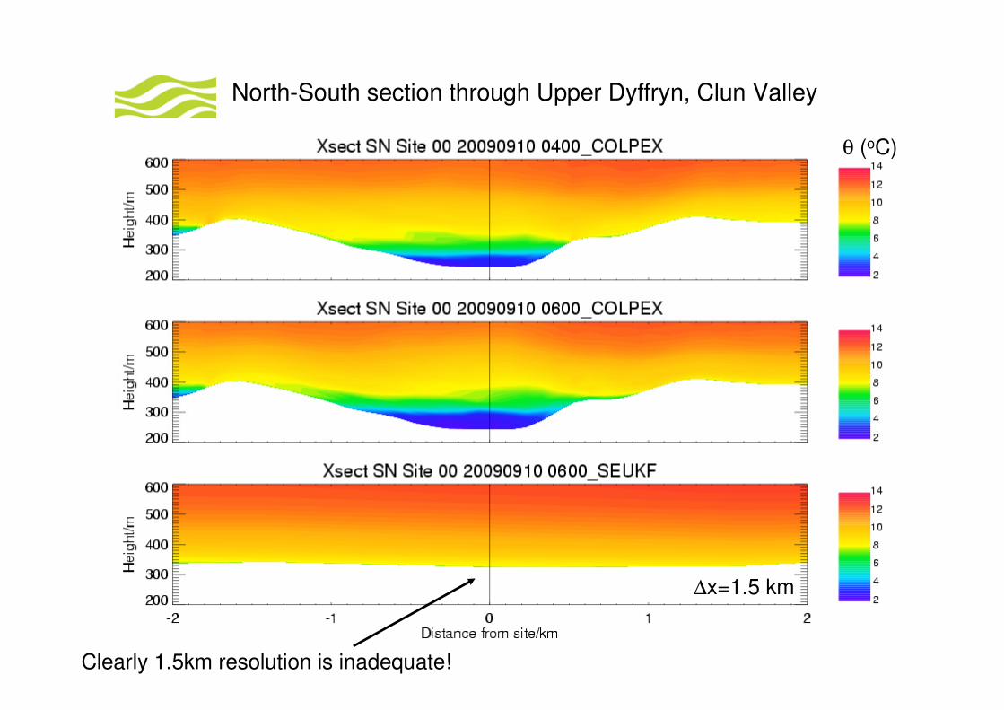
North-South section through Upper Dyffryn, Clun Valley

θ (oC)


North-South section through Upper Dyffryn, Clun Valley

θ (oC)

∆x=1.5 km

Clearly 1.5km resolution is inadequate!


Model screen temperature: ∆=100m L140 vs ∆=1.5km L70

Duffryn •Clear benefit of

100m resolution

over 1.5km or

vertical resolution?

•Temperature

minima well

represented in

high res model

•Daytime

temperatures still

too cold+-+-+obs100m L1401.5km L70


Impact of vertical resolution on screen temperature∆=100m; L140 vs L70

• L140 also improves Springhill (also by cooling slightly) and

improves Burfield by warming

Duffryn

L70 L140

20C

0C

Duffryn


SCM impact of vertical resolution is negligible!GABLSII: L70 vs L140

Wind speed

Theta

MorningEvening

ug=0.5m/s


COLPEX_100m impact of vertical resolutionL70 vs L140 at 9pm

L70

L140

SBL too turbulent?

• L140 generates realistically colder shallow SBL in valley


COLPEX_100m impact of vertical resolutionL70 vs L140 at 10pm

L70

L140

Near-surface profile now good but SBL top not perfectly defined


Surface heterogeneity: daytime (1700)• Trees/hedges 2-3K warmer than fields so gridbox

mean T will be biased warm

x

Surface heterogeneity: evening (2130)


Cold pool formation


Duffryn (Clun valley) Springhill (hill-top) Burfield (valley)

T(oC) T(oC)T(oC)

Wind speed (ms-1) Wind speed (ms-1)Wind speed (ms-1)5

0

88

0 0

-obs-model

140-level 100 m model results


Cold pool strength

• Repeatable

nighttime ∆T of

approx. -4 K

• 100m L140 model

gives good

prediction of ∆T

amplitude

• Coarser vertical

resolution (L70)

results in weaker

cold pools


Heat budget

•Q: What are the dominant sources of cooling?

•Can use the model θ budget to identify which are the

important processes at different times during the night.


•Cooling in valley is relatively rapid around sunset.•Later on, hill-top and valley cooling rates are more similar•Model heat budget suggests early rapid cooling in valley is largely due to greater turbulent heat flux divergence (relative to advection)

Model level 2 ~5m

(Advection and div.(heat flux) * 0.2)


Fog


10th-11th December 2009COLPEX IOP

11th December 00ZSatellite fog/low-cloud product

11th December 04Z


Differences in theta profiles at 1630L70 and L140 against observations

L140

Increasing resolution greatly improves vertical structure of theta profile:

• captures inversions at ~60m, ~250m and “mixed-layer” between

• again doesn’t have linear near-surface profile – too turbulent?

L70


Differences in time series of visibility, L70 and L140 against observations

• Despite better vertical T structure, L140 forms fog much earlier than L70, which was already too early

L70

L140

Observed fog onset

L140 fog onset

L70 fog onset

Compare profiles with sondes

4Z


Parametrization of cloud formation

L70

L140

• RH is (correctly) high in L140 UM over a relatively deep layer

• But there is no cloud at all in reality (from LW fluxes) despite 100% RH!

• RHcrit already set to 99% in model


N=300 cm-3 N=20 cm-3

Sensitivity to microphysics

• Fog development at Duffryn also very sensitive to assumed cloud droplet number concentration

• fewer drops are larger and so fall out faster

• leaves RH at 97-98% so potentially too dry?

Contours of qcl


UKV sensitivity to SBL mixing“LEM tails” More fog (eg eastern England)

but now too widespread and thick

Control visibility LEM tail visibility


Control: Mes tail Test: LEM tails

ModelSynop observations

Impact of LEM tails on RH distribution

• Sharper tails (less turbulent mixing) improves high end of RH distribution

• But gives too much fog

• Revise dew deposition? Improve drop number (aerosol activation)?


Summary


Summary (1)

• Diurnal cycle of screen T biases is reasonably consistent across all resolutions and timescales, suggests problems are robust

• Very active area so short term progress should be possible:

• Generally warm by night (except deserts: ε<0.97?), cold by day

• Still seen under clear skies so not exclusively a cloud problem

• Excessive nocturnal turbulent mixing (->sharper tail)

• Higher vertical resolution helps (in 100m 3D model at least)

• Excessive evaporation by day?

• Overdone direct radiative effect of aerosol?

• Surface heat capacity too large (diurnal and cloud clearing)?

• Higher soil resolution?

• Winter cold bias in screen T in high latitudes remains an issue (exacerbated by sharper tails)

• Representation of snow?

• More pronounced decoupling?

• Further analysis of surface energy budget errors and comparison with satellite surface temperatures on-going


Summary (2)

• Fog

• aerosol activation and drop number (and thence size)

• interaction with radiation (currently a fixed drop size)?

• would this (realistically) reduce the strong feedback between initial fog formation and radiative fluxes?

• improve fog deposition, including horizontally onto vegetation

• Stable boundary layers in complex terrain

• COLPEX 100m/L140 UM actually doing a remarkably good job, but much more work to be done:

• further investigation of surface temperatures and drainage flow structure

• fine details of vertical structure are important for temperature evolution and fog formation

• continue progress with understanding where and how cold pools form

• coarse-graining to inform parametrization in standard NWP configurations


Summary (3)

Unfortunately it is important to get everything right!

stable boundary layer modeling at the met office

Documents