stable boundary layer issues - ecmwf · s teeneveld, g.j.: s table boundary layer issues 26 ecmwf...

ECMWF GABLS Workshop on Diurnal cycles and the stable boundary layer, 7-10 November 2011 25

Stable Boundary Layer Issues

G.J. Steeneveld

Meteorology and Air Quality Section, Wageningen University Wageningen, The Netherlands [email protected]

Abstract

Understanding and prediction of the stable atmospheric boundary layer is a challenging task. Many physical processes are relevant in the stable boundary layer, i.e. turbulence, radiation, land surface coupling, orographic turbulent and gravity wave drag, and land surface heterogeneity. The development of robust stable boundary layer parameterizations for use in NWP and climate models is hampered by the multiplicity of processes and their unknown interactions. As a result, these models suffer from typical biases in key variables, such as 2m temperature, boundary layer depth, boundary layer wind speed. This paper summarizes the physical processes active in the stable boundary layer, their particular role, their interconnections and relevance for different stable boundary layer regimes (if understood). Also, the major model deficiencies are reported.

1. Introduction The planetary boundary layer (PBL) over land experiences a clear diurnal cycle due to the diurnal cycle of incoming radiation. From the evening transition, the Earth’s surface cools due to net longwave radiative loss. Consequently, the potential temperature increases with height, and a stable boundary layer (SBL) develops. As an illustration, Figure 1 depicts a histogram of near surface stability expressed in the bulk Richardson number (Ri) for one year (2008) of observations at the Wageningen observatory (Netherlands). For this mid-latitude station, the atmosphere is stably stratified for 51% of the time. Considering only stable conditions, the Ri distribution is heavily skewed with a median Ri of 0.01, and mean of 0.22. The 80, 90 and 95 percentiles amount 0.13, 0.49 and 1.16 respectively. The interquantile range for the SBL is much larger (0.06) than for unstable conditions (0.0036), which illustrates a wider variability within the SBL than under unstable conditions.

Figure 1: Observed histogram of near surface atmospheric stability (bulk Richardson number) at the Wageningen University Meteorological Observatory (www.maq.wur.nl), Wageningen, the Netherlands for the year 2008.

1

10

100

1000

10000

-0.5 -0.4 -0.3 -0.2 -0.1 0 0.1 0.2 0.3 0.4 0.5

Freq

uenc

y

Ri

STEENEVELD, G.J.: STABLE BOUNDARY LAYER ISSUES

26 ECMWF GABLS Workshop on Diurnal cycles and the stable boundary layer, 7-10 November 2011

The SBL is governed by a multiplicity of physical processes: turbulent mixing, radiative cooling, the interaction with the land surface, (orographically induced) gravity waves, katabatic flows, fog and dew formation etc. Despite many research efforts, these processes and their interactions are insufficiently understood, because the diversity and the usual absence of stationarity inhibits unambiguous interpretation of observations (Mahrt, 2007). Hence, this ambiguity hampers model parameterization development. As a result, the SBL is inadequately represented in atmospheric models for weather and climate (e.g. Beljaars and Viterbo, 1998; Dethloff et al., 2001; King et al., 2007; Gerbig et al., 2008; Bechtold et al., 2008, Walsh et al., 2008; Steeneveld et al. 2011; Kyselý and Plavcová, 2011).

Typical model errors for the SBL are the overestimation of the surface vegetation temperatures for calm nights (e.g. Steeneveld et al., 2008), although other models experience unrealistic decoupling of the atmosphere from the surface, resulting in so-called runaway surface cooling (e.g. Mahrt, 1998; Walsh et al., 2008). In addition, in order to obtain accurate forecast for the large scale flow, atmospheric models require more boundary-layer drag (i.e. so called long tail formulation) than can be justified from field observations. Therefore the utilized transfer functions are based on model performance rather than on a solid physical basis. Moreover, operational forecast models seem to underestimate the wind turning with height within the boundary layer (Svensson and Holtslag, 2009). Also, the SBL depth is usually too deep, and the low level jet underestimated speed and spread over an area that is deeper than typically observed. Also, models appear to underestimate the magnitude of the near surface temperature and wind speed gradient, as well as their diurnal cycle (Edwards et al., 2010). Those issues occur typically under very stable conditions. In addition, it appears that model results are very sensitive to the numerical values of certain parameters in the turbulence and orographic drag schemes (e.g. Beljaars et al, 2004; Sandu et al, 2012). Overall, a better understanding and representation of the SBL is desirable.

This paper is organised as follows. The next section summarizes the societal relevance of stable boundary layer processes. Section 3 gives an overview of the physical processes active in the stable boundary layer, their particular role, their interconnections and relevance for different stable boundary layer regimes (if understood). Finally, section 4 lists a number of further issues considering stable boundary layer over land and ice, and section provides a brief conclusion.

2. Societal Impact SBLs prevail at night, but also during daytime in winter in mid-latitudes as well as in polar regions (Yagüe and Redondo, 1995), and during daytime over irrigated regions with advection. The SBL development is relevant for numerous applications in society. For example correct forecasting of near surface temperatures and wind speed may improve the road de-icing of roads, as well as on time warnings to the transportation sector for low visibility by fog or haze at night (Van der Velde et al., 2010; Cuxart and Jiménez, 2011). Agriculture relies on accurate near surface frosts forecasts cold air pooling in order to perform measures to protect plants and yields (Prabha et al, 2011). Also, adequate air quality forecasts necessitate reliable estimates of boundary-layer depth, wind speed, and turbulence intensity (Salmond and McKendry, 2005). The same holds for CO2 inverse modeling studies (Gerbig et al., 2008). Moreover, nowadays the wind energy sector has to take hour my estimates of wind energy production, and depend on wind speed forecast, not only close to the ground, but particularly around the 100 m level (Storm and Basu, 2010).



In addition, Bony et al. (2006) found that the polar regions, that are dominantly stably stratified during a long part of the season, warm 1.4-4 times faster than the global average, but a clear reason for this is unknown. Finally the ongoing climate change is dominantly observed at night, and under stable conditions. Therefore understanding of the vertical distribution of added heat is key to interpretation of temperature at the 2 m level. Recently, Steeneveld et al. (2011) and McNider et al (2012) showed that due to feedbacks in the SBL and the land surface, the two meter temperature rise is rather constant over a relatively broad range of geostrophic wind speeds. This result means that the two meter temperature as a climate diagnostic needs to be re-discussed, as well as methods that isolate urban effects on weather stations by determining the temperature trends for different wind classes.

3. Physical Processes The complexity of the SBL originates partly from the multiplicity of processes at work. In this section the main processes are summarized, as well as their current state of knowledge, and still open issues.

3.1 Turbulence

A key characteristic of the atmospheric boundary layer is the turbulent nature of the flow. In a turbulent flow, eddies of different scales absorb energy from the mean flow. These large eddies break up to smaller eddies and finally these eddies are so small that they are dissipated by molecular viscosity. All eddy motions of different length scales, from millimetres to the scale of the boundary-layer height, transport momentum, heat, humidity and contaminants. The turbulence intensity is influenced by wind shear and stratification. During daytime the solar insolation heats the surface, and creates thermal instability and thermals. In contrast, in the SBL turbulence is suppressed by the stable stratification during calm nights. Then the turbulence is only produced by the mean wind shear; it is destroyed by buoyancy effects and (at a larger rate) viscous dissipation. As a result its energetics can be in a delicate and precarious balance, and extremely sensitive to changes in the mean wind profile (which shear is its energy source) and the mean temperature profile (which lapse rate severely limits its vertical motions).

Several turbulence regimes have been proposed within a number of SBL studies. Although they cover detailed different in regime formulations (in term of governing variables and threshold values), they all roughly distinguish between a so called “weakly stable boundary layer” (WSBL) in which turbulence is the dominant transport process, and the “very stable boundary layer” (VSBL) in which turbulence is relatively weak compared to the other processes. Within the WSBL, Nieuwstadt (1984) and many recent studies have shown that the local scaling framework, i.e. where local fluxes scale with the local gradients of wind and potential temperature, works satisfactorily. Within the VSBL a well-established scaling framework is missing. Qualitatively, this regime is determined by weak turbulence, waves, drainage flows and other (sub)mesoscale motions, that are not necessarily of local nature. Recently, Mahrt et al. (2012) found that for near-calm nocturnal conditions, significant turbulence is mainly generated by short-term (minutes) accelerations of unknown origin. Moreover, intermittent behavior of SBL turbulence (i.e. global and local intermittency) has been observed in the VSBL, but despite several proposed hypotheses of its mechanism (e.g. Nappo, 1991; Van de Wiel et al., 2003; Acevedo et al., 2011), a predictive framework is lacking for use in NWP is currently lacking.



3.2 Radiation Considering the radiation budget of the SBL, two aspects should be addressed, first the net energy balance at the surface (Q*), and secondly the radiation divergence (i.e. radiative cooling) within the atmosphere. Q* is governed by the down- and upwelling longwave radiative fluxes. The first is largely determined from the atmospheric profiles of temperature and humidity, and the latter is dominated by the surface temperature. It is important to note that Q* may experience a high frequent harmonics within the SBL, due to internal variability, but especially also just after the evening transition, when Q* shows its minimum (Van de Wiel et al., 2003). This minimum is usually a challenge for models to represent.

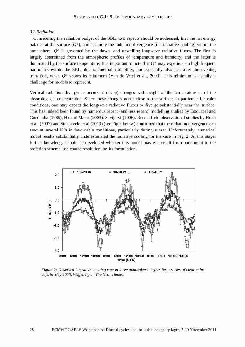
Vertical radiation divergence occurs at (steep) changes with height of the temperature or of the absorbing gas concentration. Since these changes occur close to the surface, in particular for calm conditions, one may expect the longwave radiative fluxes to diverge substantially near the surface. This has indeed been found by numerous recent (and less recent) modelling studies by Estournel and Guedahlia (1985), Ha and Mahrt (2003), Savijärvi (2006). Recent field observational studies by Hoch et al. (2007) and Steeneveld et al (2010) (see Fig 2 below) confirmed that the radiation divergence can amount several K/h in favourable conditions, particularly during sunset. Unfortunately, numerical model results substantially underestimated the radiative cooling for the case in Fig. 2. At this stage, further knowledge should be developed whether this model bias is a result from poor input to the radiation scheme, too coarse resolution, or its formulation.

Figure 2: Observed longwave heating rate in three atmospheric layers for a series of clear calm days in May 2006, Wageningen, The Netherlands.



3.3 Waves

Stratified flows allow for gravity wave propagation, due to e.g. hills and surface roughness transitions. Here, we limit ourselves to orographically induced waves. The role of propagating gravity waves in the SBL dynamics is currently under debate (e.g. Brown et al., 2003), and since NWP models still typically need more drag than can be explained by turbulence observations, alternative processes that provide drag to the flow are interesting to study and to quantify their relative contribution. Since gravity waves generate wave stress, they indeed might influence the dynamical evolution of the SBL. This mechanism is well understood for large mountain ridges. However, the SBL is shallow, and one can expect that also small-scale orography can significantly influence the SBL flow through gravity wave propagation. Nappo (2002) and Chimonas and Nappo (1989) indeed theoretically showed, using the linear theory, that the magnitude of the SBL wave stress and turbulent stress can be of the same order during weak winds.

Considering the complexity of real terrain, i.e. nonregular hills, an alternative approach to estimate τwave for these conditions is required. Figure 3 shows the estimated gravity wave drag for four contrasting nights during the CASES-99 campaign. First of all, in all nights the estimated wave drag is of the same magnitude as the measured turbulent drag. In one night 9/10 Oct the gravity wave drag is substantially larger than the turbulent drag throughout nearly the full night. In addition, we find the wave drag is highly variable throughout the night, and alternative from a finite value to zero on a timescale that is close to that of the observed global intermittent turbulence. Overall, the results in Fig. 3 suggest that orographically induced wave drag is a possible candidate to explain this missing drag.

Figure 3: Modelled surface wave stress components (lines), and measured turbulent stress (+) for a series of nights in CASES-99. In the header the classification of Van de Wiel et al. (2003) (Turb, Rad, Non) is also indicated, (Ug,Vg) indicate the geostrophic wind for the simulation.

b

d c

a



Figure 4: Ten day forecast of the diurnal cycle of near surface wind speed using a short tail, a long tail (LTG-revised), and a combined short tail and gravity wave drag scheme (a); and the change in boundary layer height using a short tail+gravity wave drag, relative to the long tailed LTG formulation (b). From: Terpstra (2010).

This suggestion is further illustrated by Fig 4 that shows the diurnal cycle of (WRF) modelled 10 m wind speed in a low pressure system over land (Europe), using three scenarios for the stability function. The run with the long tail formulation (LTG-revised) gives a small diurnal cycle, which is considered as a disadvantage of this scheme. The short tail formulation (local Monin-Obukhov) gives a larger diurnal cycle. Finally, a formulation with a short tail formulation and wave drag divergence (STGWD) in the SBL enhances the diurnal cycle with another 0.5 m/s. In addition, the nocturnal boundary-layer depth decreases by ~40 m, while not deteriorating the daytime PBL depth. The cyclone track for the three runs was approximately similar, and the deepest centre pressure appeared to be approximately 0.4 hPa lower for the ST-GWD run, than for the long tail runs. As such, the results suggest some positive impact of the ST-GWD scheme over the other schemes, i.e. a correct low pressure system representation can be combined with a realistic SBL depth and diurnal cycle for near surface wind speed. Unfortunately these results originate only from runs by a regional model and are for a single low pressure system, and as such need further confirmation.

3.4 Land surface coupling.

Considering the fact that for weak winds turbulent fluxes may vanish in the surface energy budget, the net radiation should balance the ground heat flux in order to conserve the surface energy. Hence, it is evident that the land surface coupling is important and should be well represented within atmospheric models, and its complexity should match the model complexity of parameterizations for other processes. Since the coupling with the land surface is an integral part of the SBL physics, studies using prescribed temperature, particularly with prescribed fluxes should be avoided. This aspect is further underlined in Holtslag et al. (2007), who showed that within a model intercomparison context, model output variability is strongly reduced when the atmospheric model is coupled to the land surface than for a case with prescribed surface temperature.

a b



When focusing on the Arctic, Figure 5 illustrates the EC-Earth climate model sensitivity to formulation of the snow scheme. This model, based on CY33 physics, overestimates the Arctic wintertime two meter temperature substantially, up to 6 K. On the other hand, the introduction of more realistic snow physics, based on CY36 physics, mainly causing in a stronger isolation of the atmosphere from the underlying soil, resulted in a negative temperature bias of several degrees, i.e. the bias changed a full order of magnitude. Thus, land surface coupling is a key process in very stable conditions.

Figure 5: Two meter temperature bias for Northern Hemispheric winter in EC Earth climate model (relative to ERA40), left based on ECMWF CY33 physics, and right based on ECMWF CY36 physics. Courtesy Wilco Hazeleger.

3.5 Interactions.

The above mentioned processes and their interactions have been summarized in Figure 6. The main SBL forcings are the pressure gradient force, the Coriolis force, cloud cover, and free flow stability. For example, an increased geostrophic wind speed will enhance the turbulent mixing, and thus give reduced stratification (which can also occur due to incoming clouds). A reduced stratification will reduce the magnitude of the surface sensible heat flux in the weakly stable regime, and also limit the radiation divergence and thus the clear air radiative cooling. However, in the very stable regime, a reduction of the stratification might result in increased surface sensible heat flux. In both cases the surface energy budget is also altered, resulting in a modified soil heat flux. In the case of ceasing turbulence, the magnitude of the soil heat flux increases and vice versa. Moreover, this will alter the surface temperature and therefore the outgoing long wave radiation, and so the stratification. In addition, increased geostrophic wind will under certain conditions increase the impact of wave drag due to the orography, which at first increases the cyclone filling and thus reduces the geostrophic wind. On the other hand, it will also enhance the low-level jet wind speed. This consequently might result in additional downward turbulent mixing from the jet. This starts to affect the stratification again.



Figure 6: Schematic overview of physical processes in the stable boundary layer over land, including their interactions and positive (____) and negative feedbacks (-----).

4. Some further issues. First the role of horizontal diffusion is discussed. Under very stable conditions, meandering motions have been frequently observed, but their representation in atmospheric models has been limited. Belušić and Güttler (2010) evaluated the skill of the mesoscale model WRF to reproduce these meandering flows within the SBL. As illustrated in Fig. 7, they found a relatively strong sensitivity to the parameterization of horizontal diffusion. Using the reference settings with relatively much horizontal diffusion, both time series and power spectral density evidently diverged from observations, with a much smoother signal than observed (blue line in Fig. 7). Neglecting horizontal diffusion resulted in a power spectrum with more variability than was observed. Using a constant, but small, horizontal diffusion coefficient, a reasonable agreement with observations, and submeso variability was found. Belušić and Güttler (2010) also found a strong impact of the horizontal diffusion on the atmospheric concentration of species, with a more realistic pattern using horizontal diffusion smaller than the reference value. Overall, these results suggest further study towards a robust formulation of horizontal diffusion is relevant to and can be fruitful for SBL modelling.



Figure 7: Modelled (mesoscale model WRF) and observed (CASES-99) horizontal wind speed (left) and power spectral density for a relative calm night (from: Belušić and Güttler, 2010)

Second, we discuss a so far unresolved issue, which is whether the above listed SBL problems are consistent different levels in the model hierarchy. Several studies have shown stable conditions can be well represented within the single column models when the local forcing conditions (geostrophic wind speed) and landuse properties are well known (e.g. Steeneveld et al., 2006; Baas et al., 2010). Hence, these studies suggest that the reported modelling errors are more strongly visible in 3D models than in 1D models. Therefore it would be illustrative to document SBL model bias relative to model hierarchy.

Finally, another important aspect to mention is the lack of understanding and model skill over the Arctic regions. A model evaluation study reported in Walsh et al. (2008) showed a wide variety of model skill for the 2 m temperature. Some models produced significant cold bias, while others gave a substantial warm bias. In addition, Meideros et al (2011) report a significant overestimation of the Arctic inversion strength in the CMIP3 models. As such, a clear need exist to isolate and quantify the relative role of the different processes relevant to the Arctic.

5. Conclusion The stable boundary layer is governed by multiple processes. The weakly stable boundary layer is dominated by well-defined turbulence that follows local scaling, and this regime can be relatively well modelled and forecasted. Within the very stable regime processes as radiation divergence, orographic drag, land surface coupling and (sub)mesoscale motions. These processes have not been fully understood and their relative impact has not been quantified yet. However, in terms of model development, process splitting should be preferred over an approach that lumps all processes together within the stability function in the boundary layer scheme.

Acknowledgements

The author acknowledges NWO VENI grant “Lifting the fog” (contract number 863.10.010), and all co-workers who contributed to this chapter, i.e. Bert Holtslag, Bas van de Wiel, Wilco Hazeleger, Annick Terpstra, Bert Heusinkveld, Christine Groot Zwaaftink, Marcel Wokke, Sander Pijlman, Carmen Nappo.



References

Baas P., F.C. Bosveld, G. Lenderink, E. van Meijgaard, A.A.M. Holtslag, 2010: How to design single column model experiments for comparison with observed nocturnal low-level jets, Q. J. R. Meteorol. Soc.136, 671–684.

Bechtold, P., M. Köhler, T. Jung. F. Doblas-Reys, M. Letbecher, M.J. Rodwell, R. Vitart, and G. Balsamo, 2008: Advances in simulating atmospheric variability with the ECMWF model: From synoptic to decadal time-scales. Quart. J. Roy. Meteor. Soc., 134, 1337-1351.

Beljaars, A.C.M., A.R. Brown, and N. Wood, 2004: A new parameterization of turbulent orographic form drag, Quart. J. Roy. Meteor. Soc., 130, 1327-1347.

Belušić, D., and I. Güttler, 2010: Can mesoscale model reproduce meandering motions?, Quart J. Roy Meteor. Soc., 136, 553-565.

Bony, S. and co-authors, 2006: How well do we understand and evaluate climate change feedback processes? J. Climate, 19, 3445-3482.

Brown, A.R., M. Athanassiadou, and N. Wood, 2003: Topographically induced waves within the stable boundary layer, Quart. J. Roy. Meteor. Soc., 129, 3357-3370.

Chimonas, G. and C.J. Nappo, 1989: Wave drag in the planetary boundary layer over complex terrain, Bound.-Layer Meteor., 47, 217-232.

Cuxart, J. and M.A. Jiménez, 2011: Deep Radiation Fog in a Wide Closed valley: Study by Numerical Modeling and Remote Sensing, Pure Appl. Geophys., in press, doi: 10.1007/s00024-011-0365-4.

Dethloff, K., C. Abegg, A. Rinke, I. Hebestadt, and V.F. Romanov, 2001: Sensitivity of Arctic climate simulations to different boundary-layer parameterizations in a regional climate model. Tellus, 53A, 1-26.

Dutra, E., G. Balsamo, P. Viterbo, P.M.A. Miranda, A. Beljaars, C. Schär, K. Elder, 2010: An improved snow scheme for the ECMWF land surface model: description and offline validation. J. Hydrometeor, 11, 899-916.

Edwards, J.M., J.R. McGregor, M.R. Bush, F.J.A. Bornemann, 2011: Assessment of numerical weather forecasts against observations from Cardington: Seasonal diurnal cycles of screen-level and surface temperatures and surface fluxes, Quart. J. Roy. Meteorol. Soc., 137, 656-672.

Estournel, C. and D. Guedalia, 1985: Influence of geostrophic wind on atmospheric nocturnal cooling, J. Atmos. Sci., 42, 2695-2698.

Gerbig, C., S. Körner, and J.C. Lin, 2008: Vertical mixing in atmospheric tracer transport models: error characterization and propagation. Atmos. Chem. Phys., 8, 591-602.

Ha, K.J. and L. Mahrt, 2003: Radiative and turbulent fluxes in the nocturnal boundary layer, Tellus, 55A, 317-327.

Hoch, S.W., P. Calanca, R. Philipona, and A. Ohmura, 2007: Year-Round Observation of Longwave Radiative Flux Divergence in Greenland. J. Appl. Meteor. Clim., 45, 1469-1479.

Holtslag, A.A.M., G.J. Steeneveld, and B.J.H. van de Wiel, 2007: Role of land-surface feedback on model performance for the stable boundary layer, Bound. Layer. Meteorol., 125, 361-376.

King, J.C., W.M. Connolley and S.H. Derbyshire, 2001: Sensitivity of modelled Antarctic climate to surface flux and boundary-layer flux parameterizations, Quart. J. Roy. Meteor. Soc.., 127, 779-794.



Kyselý, J., and E. Plavcová, 2011: Biases in the diurnal temperature range in Central Europe in an ensemble of regional climate models and their possible causes. Clim. Dyn., in press.

Mahrt, L., 2007: Weak-wind mesoscale meandering in the nocturnal boundary layer, Env. Fluid Mech., 7, 331-347.

Mahrt L, Richardson S, Seaman N, Stauffer D. 2012. Turbulence in the nocturnal boundary layer with light and variable winds. Q. J. R. Meteorol. Soc. In press. DOI:10.1002/qj.1884.

Medeiros, B., C. Deser, R.A. Tomas, J.E. Kay, 2011: Arctic inversion strength in climate models. J. Climate, 24, 4733-4740.

McNider, R.T., G.J. Steeneveld, A.A.M. Holtslag, R.A. Pielke Sr., S. Mackaro, A. Pour-Biazar, J. Walters, U. Nair and J. Christy, 2012: Reponse and Sensitivity of the Nocturnal Boundary Layer over Land to Added Radiative Forcing, in preparation.

Nappo, C.J., 1991: Sporadic breakdowns of stability in the PBL over simple and complex terrain, Bound.-Layer Meteor., 54, 69-87.

Nappo, C.J., 2002: An Introduction to Atmospheric Gravity Waves, Academic Press, London, 276 pp.

Nieuwstadt, F.T.M., 1984: The turbulent structure of the stable, nocturnal boundary layer, J. Atmos. Sci., 41, 2202-2216.

Prabha, T.V., Hoogenboom, G., Smirnova, T.G., 2011: Role of land surface parameterizations on modeling cold-pooling events and low-level jets, Atmos. Res., 99, 147-161.

Salmond, J.A. and I.G. McKendry, 2005: A review of turbulence in the very stable boundary layer and its implications for air quality, Progress in Phys. Geography, 29, 171-188.

Sandu, I, et al, 2012: Experience with boundary layer formulations in the ECMWF model. This issue chapter X.

Savijarvi, H., 2006: Radiative and turbulent heating rates in the clear-air boundary layer, Quart. J. Roy. Met. Soc., 132, 147-161.

Steeneveld, G.J., A.A.M. Holtslag, C.J. Nappo and L. Mahrt, 2008: Exploring the role of small-scale gravity wave drag on stable boundary layers over land, J. Appl. Meteor. Clim., 47, 2518–2530.

Steeneveld, G.J., M.J.J. Wokke, C.D. Groot Zwaaftink, S. Pijlman, B.G. Heusinkveld, A.F.G. Jacobs, A.A.M. Holtslag, 2010: Observations of the radiation divergence in the surface layer and its implication for its parametrization in numerical weather prediction models. J. Geophys Res., 115, D06107, doi:10.1029/2009JD013074.

Steeneveld, G.J., C.J. Nappo, and A.A.M. Holtslag, 2009: Estimation of orographically induced wave drag in the stable boundary layer during CASES99, Acta Geophys., 57, 857-881.

Steeneveld, G.J., A.A.M. Holtslag, R.T. McNider, R.A. Pielke, 2011: Screen level temperature increase due to higher atmospheric carbon dioxide in calm and windy nights revisited, J. Geophys. Res., 116, D02122, doi:10.1029/2010JD014612.

Storm, B., and S. Basu, 2010: The WRF Model Forecast-Derived Low-Level Wind Shear Climatology over the United States Great Plains, Energies, 3, 258-276.

Svensson G, Holtslag AAM. 2009. Analysis of model results for the turning of the wind and related momentum fluxes in the stable boundary layer. Boundary-Layer Meteorol. 132, 261–277.

Terpstra, A., 2011: Orographic gravity wave drag in the stable boundary layer: influence on cyclone filling and boundary layer features, MSc thesis report, Wageningen University, Wageningen, Netherlands, 33p.



Walsh, J.E., W.L., Chapman, V. Romanovsky, J.H. Christensen, and M. Stendel, 2008: Global Climate Model Performance over Alaska and Greenland. J. Climate. 21, 6156-6174.

Wiel, B.J.H. van de, A.F. Moene, O.K. Hartogensis, H.A.R. de Bruin, and A.A.M. Holtslag, 2003: Intermittent turbulence and oscillations in the stable boundary-layer over land. Part III: a classification for observations during CASES99. J. Atmos. Sci., 60, 2509-2522.

Velde, I.R. van der, G. J. Steeneveld, B.G.J. Wichers Schreur, and A.A.M. Holtslag, 2010: Modeling and forecasting the onset and duration of severe radiation fog under frost conditions, Mon. Wea. Rev., 138, 4237-4253.

Yague, C., and J.M. Redondo, 1995: A case study of turbulent parameters during the Antarctic winter, Antarctic Sci., 7, 421-433.

stable boundary layer issues - ecmwf · s teeneveld, g.j.: s table boundary layer issues 26 ecmwf...

Documents