stability of high order ﬁnite diﬀerence schemes with

Stability of high order finite difference schemes with implicit-explicit

time-marching for convection-diffusion and convection-dispersion equations

Meiqi Tan1, Juan Cheng2, and Chi-Wang Shu3

Abstract

The main purpose of this paper is to analyze the stability of the implicit-explicit (IMEX)

time-marching methods coupled with high order finite difference spatial discretization for

solving the linear convection-diffusion and convection-dispersion equations in one dimen-

sion. Both Runge-Kutta and multistep IMEX methods are considered. Stability analysis

is performed on the above mentioned schemes with uniform meshes and periodic boundary

condition by the aid of the Fourier method. For the convection-diffusion equations, the re-

sult shows that the high order IMEX finite difference schemes are subject to the time step

restriction ∆t ≤ max{τ0, c∆x}, where τ0 is a positive constant proportional to the diffu-

sion coefficient and c is the Courant number. For the convection-dispersion equations, we

show that the IMEX finite difference schemes are stable under the standard CFL condition

∆t ≤ c∆x. Numerical experiments are also given to verify the main results.

Keywords: Convection-diffusion equation; Convection-dispersion equation; Stability;

IMEX; finite difference; Fourier method

1Graduate School, China Academy of Engineering Physics, Beijing 100088, China. E-mail: tan-

[email protected] of Computational Physics, Institute of Applied Physics and Computational Mathematics,

Beijing 100088, China and Center for Applied Physics and Technology, Peking University, Beijing 100871,

China. E-mail: cheng [email protected]. Research is supported in part by NSFC grants 11871111, 12031001

and U1630247, Science Challenge Project. No. TZ2016002, and CAEP Foundation No. CX20200026.3Division of Applied Mathematics, Brown University, Providence, RI 02912. E-mail: chi-

wang [email protected]. Research is supported in part by NSF grant DMS-2010107 and AFOSR grant FA9550-

20-1-0055.

1

1 Introduction

In this paper, the stability property of the high order finite difference schemes with certain

implicit-explicit (IMEX) time-marching methods is studied for the convection-diffusion and

convection-dispersion equations respectively. For the spatial derivative terms of these equa-

tions, we use a high order upwind biased finite difference scheme, which is a prototype of the

weighted essentially non-oscillatory (WENO) schemes [8,13,15], to discretize the convection

term, a high order central difference method to discretize the diffusion term, and a high

order upwind biased finite difference scheme to discretize the dispersion term.

The time derivative term for the convection-diffusion and convection-dispersion equations

should be discretized carefully. If explicit time-marching methods are used, then the time

step is dominated by the highest order derivative term, which may be very small, result-

ing in excessive computational cost. For example, for the convection-dispersion equations

involving third order spatial derivatives which are not convection-dominated, the explicit

time discretization may suffer from a strict time step restriction ∆t ∼ O(∆x3) for stability,

where ∆t is the time step and ∆x is the spatial mesh size. If the fully implicit time-marching

methods are used, then the time step restriction may be relaxed, and usually unconditionally

stable such as A-stable schemes can be designed. However, in many practical applications

the lower order convection terms are often nonlinear, hence the implicit methods may be

much more expensive per time step than the explicit methods, because an iterative solution

of the nonlinear algebraic equations is needed.

When it comes to such problems, a natural consideration is to treat different derivative

terms differently, that is, the higher order derivative terms are treated implicitly, whereas

the rest of the terms are treated explicitly. The IMEX time-marching methods, which have

been proposed and studied by many authors [1–7, 10, 11, 14, 17, 18], have considered such

a strategy. This can not only alleviate the stringent time step restriction, but also reduce

the difficulty of solving the algebraic equations, especially when the higher order derivative

terms are linear. Even when the higher order derivative terms are nonlinear, the IMEX

2

time-marching methods might still show their advantages in obtaining a better algebraic

system, for example for diffusive higher order derivatives the algebraic system might have

some symmetry and positive definite properties, which can be easily solved by many iterative

methods.

For the convection-diffusion equations, there have been many studies in the literature on

the IMEX methods. In [1], a pair of multistep IMEX time-marching methods are constructed.

Coupled with the traditional second order central difference method, the multistep IMEX fi-

nite difference schemes are shown to be stable under the standard CFL condition ∆t ≤ c∆x,

where c is the Courant number. However, most of them tend to have an undesirably small c,

unless diffusion strongly dominates and an appropriate backward differentiation formula is

selected for the diffusion term. In [10], the authors designed several stable multistep IMEX

time discretizations, which are specially tailored for stability when coupled with the pseu-

dospectral method. These schemes are shown to be stable provided that the time step and

the spatial mesh size are bounded by two constants. Combined with the local discontinuous

Galerkin (LDG) method, a variety of IMEX schemes [17, 18], including Runge-Kutta type

and multistep type IMEX schemes, have been discussed. These schemes are stable provided

that the time step is upper-bounded by a positive constant τ0 which is proportional to d/ν2,

where ν and d are the convection and diffusion coefficients, respectively. However, when d

is very small in comparison with the spatial mesh size, τ0 is too small to be the true bound

for stability. For the above mentioned equations without the diffusion terms, the explicit

scheme is usually stable under the standard CFL condition. We could therefore reasonably

expect that the IMEX method for this convection-diffusion equation should also be stable

under the same CFL condition. The schemes in [19], where the explicit part is treated by

a strong-stability-preserving Runge-Kutta method [9], and the implicit part is treated by

an L-stable diagonally implicit Runge-Kutta method, are also subject to the time step re-

striction ∆t ≤ τ0. They also face the problem that τ0 is too small to be the true bound for

stability when d is very small in comparison with the spatial mesh size.

3

For the convection-dispersion equations, there are also some studies in the literature on

the IMEX methods. In [6], some multistep IMEX time-marching methods with the spectral

spatial discretization for the KdV equation have been presented. Coupled with the finite

volume spatial discretization, some IMEX Runge-Kutta methods are tested in the case of

the KdV equation in [5]. These schemes are shown to be stable under the standard CFL

condition ∆t ≤ c∆x. In [11], the IMEX method with the discontinuous Galerkin (DG)

spatial discretization is proposed for the KdV equation, where the stability analysis is not

discussed.

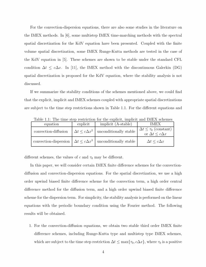
If we summarize the stability conditions of the schemes mentioned above, we could find

that the explicit, implicit and IMEX schemes coupled with appropriate spatial discretizations

are subject to the time step restrictions shown in Table 1.1. For the different equations and

Table 1.1: The time step restriction for the explicit, implicit and IMEX schemesequation explicit implicit (A-stable) IMEX

convection-diffusion ∆t ≤ c∆x2 unconditionally stable∆t ≤ τ0 (constant)

or ∆t ≤ c∆x

convection-dispersion ∆t ≤ c∆x3 unconditionally stable ∆t ≤ c∆x

different schemes, the values of c and τ0 may be different.

In this paper, we will consider certain IMEX finite difference schemes for the convection-

diffusion and convection-dispersion equations. For the spatial discretization, we use a high

order upwind biased finite difference scheme for the convection term, a high order central

difference method for the diffusion term, and a high order upwind biased finite difference

scheme for the dispersion term. For simplicity, the stability analysis is performed on the linear

equations with the periodic boundary condition using the Fourier method. The following

results will be obtained.

1. For the convection-diffusion equations, we obtain two stable third order IMEX finite

difference schemes, including Runge-Kutta type and multistep type IMEX schemes,

which are subject to the time step restriction ∆t ≤ max{τ0, c∆x}, where τ0 is a positive

4

constant proportional to the diffusion coefficient and c is the Courant number;

2. For the convection-dispersion equations, we obtain two stable third order IMEX Runge-

Kutta finite difference schemes and a second order multistep IMEX finite difference

scheme, which are subject to the time step restriction ∆t ≤ c∆x, where c is the Courant

number.

Although the stability analysis is performed on linear equations, the schemes are also appli-

cable to nonlinear equations which will be demonstrated by numerical tests.

The organization of this paper is as follows. In Section 2, we will present two IMEX

finite difference schemes for the linear convection-diffusion equation, and will concentrate on

the stability analysis of the corresponding schemes. Numerical experiments are also given to

demonstrate the stability results given by our analysis. In Section 3, we will provide several

numerical examples, including linear and nonlinear equations, to numerically validate the

stability condition and the error accuracy for the schemes. Section 4 is similar to Section 2,

and Section 5 is similar to Section 3, but they are for the convection-dispersion equations.

Finally, the concluding remarks are presented in Section 6.

2 The IMEX finite difference schemes for the convection-

diffusion equations

Consider the linear convection-diffusion equation

{

ut + ux = duxx, (x, t) ∈ (a, b) ∪ (0, T ]

u(x, 0) = u0(x), x ∈ [a, b](2.1)

with periodic boundary condition, where d ≥ 0 is the diffusion coefficient. Assume that [a, b]

is uniformly partitioned into N cells with the spatial mesh size given by ∆x = b−aN

. For

the spatial discretization, we use the third order upwind biased finite difference scheme for

the convection term, which is just the standard third order WENO scheme with the linear

weights, and the fourth order central difference method for the diffusion term to get the

5

semidiscrete scheme,

du

dt

∣

∣

∣

∣

x=xi

= L(t, u)i +N(t, u)i (2.2)

in which N(t, u)i represents the spatial discretization of the convection term

N(t, u)i = −3ui + 2ui+1 − 6ui−1 + ui−2

6∆x(2.3)

and L(t, u)i represents the spatial discretization of the diffusion term

L(t, u)i = d−(ui+2 + ui−2) + 16(ui+1 + ui−1)− 30ui

12∆x2(2.4)

The numerical solution ui approximates the exact solution u(t, xi) at the grid point xi. In

the following subsections, we will consider two types of IMEX time-marching methods, i.e.,

Runge-Kutta and multistep methods given in [18]. We will give the stability analysis on these

two high order IMEX methods coupled with the above finite difference spatial discretization

by the Fourier method. Numerical experiments are also given to demonstrate the stability

results given by our analysis.

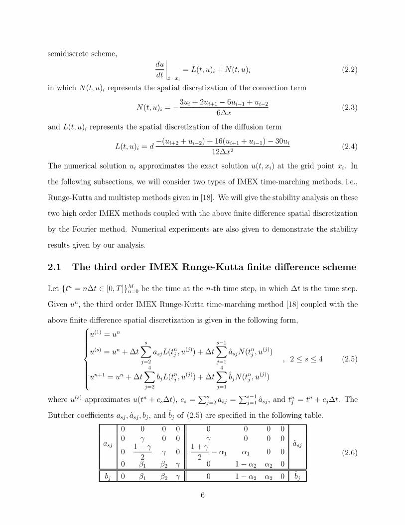
2.1 The third order IMEX Runge-Kutta finite difference scheme

Let {tn = n∆t ∈ [0, T ]}Mn=0 be the time at the n-th time step, in which ∆t is the time step.

Given un, the third order IMEX Runge-Kutta time-marching method [18] coupled with the

above finite difference spatial discretization is given in the following form,

u(1) = un

u(s) = un +∆t

s∑

j=2

asjL(tnj , u

(j)) + ∆t

s−1∑

j=1

asjN(tnj , u(j))

un+1 = un +∆t4

∑

j=2

bjL(tnj , u

(j)) + ∆t4

∑

j=1

bjN(tnj , u(j))

, 2 ≤ s ≤ 4 (2.5)

where u(s) approximates u(tn + cs∆t), cs =∑s

j=2 asj =∑s−1

j=1 asj, and tnj = tn + cj∆t. The

Butcher coefficients asj, asj, bj , and bj of (2.5) are specified in the following table.

asj

0 0 0 0 0 0 0 0

asj0 γ 0 0 γ 0 0 0

01− γ

2γ 0

1 + γ

2− α1 α1 0 0

0 β1 β2 γ 0 1− α2 α2 0

bj 0 β1 β2 γ 0 1− α2 α2 0 bj

(2.6)

6

The left half of the table lists asj and bj , with the four rows from top to bottom corresponding

to s = 1, 2, 3, 4, and the columns from left to right corresponding to j = 1, 2, 3, 4. Similarly,

the right half lists asj and bj in (2.6), γ ≈ 0.435866521508459, β1 = −32γ2 + 4γ − 1

4and

β2 =32γ2 − 5γ + 5

4. The parameter α1 is chosen as −0.35 in [17] and α2 =

1

3−2γ2

−2β2α1γ

γ(1−γ).

2.1.1 Stability analysis

We know that when the spatial discretization operator is LDG, the IMEX schemes [17,18] are

shown to be stable as long as the time step is upper-bounded by a constant, which depends

on the ratio of the diffusion coefficient and the square of the convection coefficient. For the

IMEX Runge-Kutta finite difference scheme (2.5), we expect to obtain similar stability, that

is, the scheme could be stable under the condition ∆t ≤ τ0, where τ0 is a positive constant

depending solely on the diffusion coefficient d (notice that the convection coefficient is the

constant 1). Next, we would like to explore whether the scheme would allow us to achieve

such stability by the aid of the Fourier method.

The Fourier method, which is a powerful tool for stability analysis, consists of examining

the following Fourier modes

unj = vneIkxj , I2 = −1. (2.7)

for appropriate wave number k. Substituting (2.7) into (2.5) yields

vn+1 = Gvn. (2.8)

where the amplification factor G is a function of k,∆x,∆t, d. The specific formula of G for

the scheme (2.5) is listed in Appendix A. The necessary and sufficient stability condition on

G is given by the following theorem.

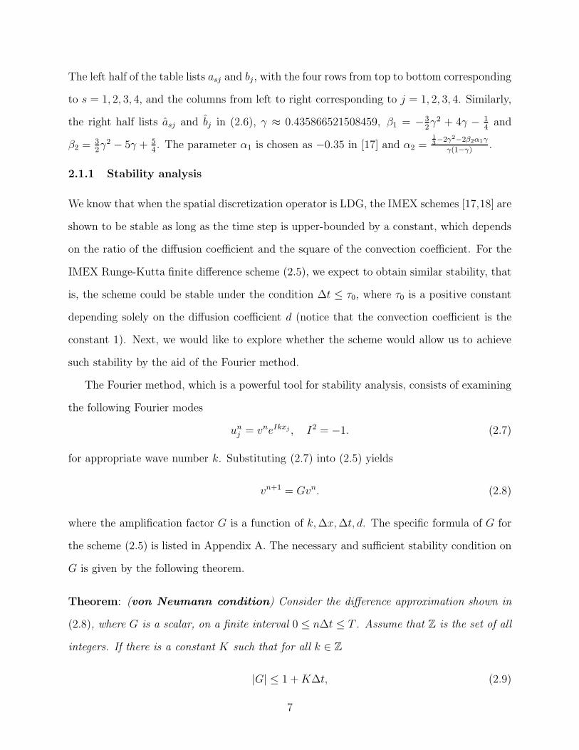
Theorem: (von Neumann condition) Consider the difference approximation shown in

(2.8), where G is a scalar, on a finite interval 0 ≤ n∆t ≤ T . Assume that Z is the set of all

integers. If there is a constant K such that for all k ∈ Z

|G| ≤ 1 +K∆t, (2.9)

7

then the approximation is stable.

Because the L2 norm of the exact solution to the equation (2.1) does not increase in time,

we would look for strong stability, namely the von Neumann stability requirement is |G| ≤ 1.

If |G| ≤ 1 holds for ∆t ≤ τ0, then the scheme is stable under the condition ∆t ≤ τ0. If τ0 is

a sharp bound, then |G| will be greater than 1 when ∆t = τ0+ ε (we take varepsilon = 0.01

in our tests). As shown in Appendix A, the specific formula for G is very complex. Thus it

is difficult to obtain τ0 analytically. Considering the algebraic complexity, we will try to get

it numerically. The specific procedure to obtain τ0 is as follows.

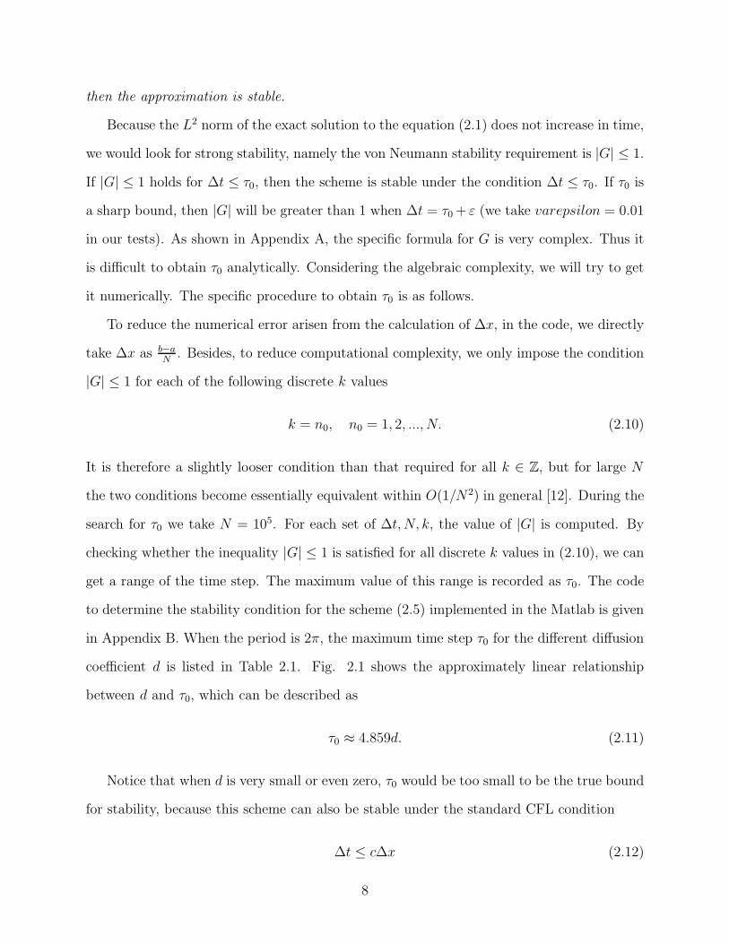
To reduce the numerical error arisen from the calculation of ∆x, in the code, we directly

take ∆x as b−aN

. Besides, to reduce computational complexity, we only impose the condition

|G| ≤ 1 for each of the following discrete k values

k = n0, n0 = 1, 2, ..., N. (2.10)

It is therefore a slightly looser condition than that required for all k ∈ Z, but for large N

the two conditions become essentially equivalent within O(1/N2) in general [12]. During the

search for τ0 we take N = 105. For each set of ∆t, N, k, the value of |G| is computed. By

checking whether the inequality |G| ≤ 1 is satisfied for all discrete k values in (2.10), we can

get a range of the time step. The maximum value of this range is recorded as τ0. The code

to determine the stability condition for the scheme (2.5) implemented in the Matlab is given

in Appendix B. When the period is 2π, the maximum time step τ0 for the different diffusion

coefficient d is listed in Table 2.1. Fig. 2.1 shows the approximately linear relationship

between d and τ0, which can be described as

τ0 ≈ 4.859d. (2.11)

Notice that when d is very small or even zero, τ0 would be too small to be the true bound

for stability, because this scheme can also be stable under the standard CFL condition

∆t ≤ c∆x (2.12)

8

Table 2.1: The maximum time step τ0.d 0 0.0001 0.001 0.01 0.05 0.1 0.2 0.3 0.4 0.5τ0 0 0.0005 0.004 0.04 0.24 0.48 0.97 1.45 1.94 2.43

Figure 2.1: The fitting curve of the maximum time step τ0 and the diffusion coefficient d.

if the diffusion term is not considered. Next, we would like to further find the possible

CFL-like stability condition (2.12) for the scheme (2.5).

Similarly, we obtain c in (2.12) numerically. When d = 0, we get the Courant number c

as follows,

c = 1.3599. (2.13)

We also observe the following two important facts.

1. When max{c∆x, τ0} = τ0, |G| ≤ 1 holds. When ∆t = τ0+0.01, |G| tends to be greater

than 1.

2. For d > 0, we find that c = 1.3599 may not be the optimal Courant number; that is,

|G| may not be greater than 1 if we take ∆t = (c + 0.01)∆x. But for any d, it seems

sufficient to ensure that if ∆t = max{c∆x, τ0} = c∆x, then |G| ≤ 1.

Therefore, we conclude that the third order IMEX Runge-Kutta finite difference scheme

9

(2.5) is stable under the condition

∆t ≤ max{τ0, c∆x} (2.14)

where τ0 ≈ 4.859d, c = 1.3599.

In order to further verify whether the scheme is subject to the above time step restriction,

we consider the following equation

{

ut + ux = duxx, (x, t) ∈ (−π, π) ∪ (0, T ]

u(x, 0) = sin x, x ∈ [−π, π](2.15)

with periodic boundary condition. The exact solution of (2.15) is u(x, t) = e−dt sin(x − t).

We use the scheme (2.5) to solve the above equation.

On the one hand, we take Nτ0 = 640 in the tests so that max{c∆x, τ0} = τ0, where

∆x = 2πNτ0

. For any fixed diffusion coefficient d, we take ∆t as τ0 − 0.01, τ0 and τ0 + 0.01,

respectively. Table 2.2 lists the L1 error of the scheme (2.5) for solving (2.15) with the

different time step. As expected, the error will blow up if we take ∆t = τ0+0.01 but is small

when ∆t ≤ τ0. Therefore, when max{c∆x, τ0} = τ0, τ0 is the precise bound of the time step

restriction for stability. This clearly demonstrates the stability result (2.14) given by our

analysis in such situation.

On the other hand, we take Nc = 40 in the tests such that max{c∆x, τ0} = c∆x, where

∆x = 2πNc. For any given diffusion coefficient d, we take the time step ∆t as (c − 0.01)∆x,

c∆x and (c + 0.01)∆x, respectively. We can clearly observe from Table 2.3 that when d is

small enough, the error will blow up if we take ∆t = (c + 0.01)∆x but is tolerable under

the condition ∆t ≤ c∆x, and when d is relatively larger, the error will not blow up when

∆t = (c+ 0.01)∆x, which verifies our observation in the stability analysis.

Thus, combining the results in Table 2.2-2.3, we conclude that the third order IMEX

Runge-Kutta finite difference scheme (2.5) is stable under the time step restriction (2.14).

10

Table 2.2: The error of the scheme (2.5) for solving the equation (2.15) with the differenttime step in the case of max{τ0, c∆x} = τ0, ∆x = 2π

Nτ0

.

d ∆t Nτ0 T L1 error

d=0.52.42

640 500009.10E-14

2.43 2.04E-142.44 2.63E+16

d=0.41.93

640 500005.12E-14

1.94 2.91E-141.95 4.13E+07

d=0.20.96

640 100008.19E-15

0.97 6.74E-150.98 5.32E+08

Table 2.3: The error of the scheme (2.5) for solving the equation (2.15) with the differenttime step in the case of max{τ0, c∆x} = c∆x, ∆x = 2π

Nc.

d ∆t Nc T L1 error

d=01.3499∆x

40 100000.537

1.3599∆x 0.5391.3699∆x 3.88E+217

d=0.00011.3499∆x

40 100000.1975

1.3599∆x 0.19821.3699∆x 4.61E+157

d=0.0011.3499∆x

40 1000002.52E-16

1.3599∆x 4.68E-161.3699∆x 2.87E-16

d=0.011.3499∆x

40 1000001.61E-16

1.3599∆x 1.58E-161.3699∆x 1.13E-16

11

2.2 The third order multistep IMEX finite difference scheme

Considering the semidiscrete scheme (2.2), we use the third order multistep IMEX time-

marching method given in [18] to discretize it to obtain a finite difference scheme as follows

un+1i =un

i +∆t(23

12N(tn, un)i −

4

3N(tn−1, un−1)i +

5

12N(tn−2, un−2)i

)

+∆t(2

3L(tn+1, un+1)i +

5

12L(tn−1, un−1)i −

1

12L(tn−3, un−3)i

)

(2.16)

where N(t, u)i and L(t, u)i are defined as (2.3) and (2.4) respectively. Next, we will perform

the stability analysis on this scheme.

2.2.1 Stability analysis

When the spatial discretization operator is LDG, we know that the multistep IMEX schemes

[18] are shown to be stable provided that the time step is upper-bounded by a positive con-

stant, which depends on the ratio of the diffusion coefficient and the square of the convection

coefficient. For the multistep IMEX finite difference scheme (2.16), we expect to obtain sim-

ilar stability, that is, the scheme could also be stable under the condition ∆t ≤ τ0, where

τ0 is a positive constant proportional to the diffusion coefficient d. Next, we would like to

explore whether the scheme can achieve such stability by the aid of the Fourier method.

Substituting the Fourier modes (2.7) into the scheme, we obtain

vn+1 = a1vn + a2v

n−1 + a3vn−2 + a4v

n−3 (2.17)

The specific formulas for ai, i = 1, .., 4 are listed in Appendix A.

To solve (2.17), we make the ansatz

vn = zn (2.18)

where z is a complex number. Substituting (2.18) into (2.17) gives us

zn+1 − a1zn − a2z

n−1 − a3zn−2 − a4z

n−3 = 0 (2.19)

Therefore, (2.18) is a solution of (2.17) if, and only if, z satisfies the so called characteristic

equation

z4 − a1z3 − a2z

2 − a3z − a4 = 0. (2.20)

12

The necessary and sufficient stability condition on the characteristic root z is defined as

follows.

Theorem: Consider the difference approximation shown in (2.17) on a finite interval 0 ≤

n∆t ≤ T . Assume that Z is the set of all integers. If there is a constant K such that for all

k ∈ Z{

|z| < 1, if z is a multiple root

|z| ≤ 1 +K∆t, else(2.21)

then the approximation is stable.

Applying to the case of interest here, we would like to derive the values of τ0 for strong

stability, namely{

|z| ≤ 1, when z is a simple root of (2.20).

|z| < 1, when z is a multiple root of (2.20).(2.22)

since the L2 norm of the exact solution to the equation (2.1) does not increase in time.

Considering the algebraic complexity, we still get τ0 numerically. When the period is 2π,

the maximum time step τ0 is obtained in the similar way as that for the third order IMEX

Runge-Kutta finite difference scheme (2.5). We refer to Section 2.1.1 for more details. Here

we just summarize the result in Table 2.4.

Table 2.4: The maximum time step τ0.d 0 0.001 0.01 0.05 0.1 0.2 0.3 0.4 0.5τ0 0 0.0002 0.002 0.012 0.025 0.051 0.077 0.102 0.128

Similarly Fig.2.2 shows the approximately linear relationship between d and τ0, which

can be expressed as

τ0 ≈ 0.2566d. (2.23)

We observe that the IMEX Runge-Kutta finite difference scheme (2.5) admits larger time

step than the multistep IMEX finite difference scheme (2.16). Similar to the scheme (2.5),

when d is very small in comparison with the spatial mesh size, τ0 determined by (2.23) is

too small to be true for stability. Thus, we will further find the similar CFL-like stability

condition for the scheme (2.16).

13

Figure 2.2: The fitting curve of the maximum time step τ0 and the diffusion coefficient d.

In order to get stability, c should satisfy (2.22). We get the value of c numerically. When

d = 0, we obtain c = 0.39, that is, the scheme is stable when the time step satisfies

∆t ≤ 0.39∆x. (2.24)

Besides, we also observe the following two important facts.

1. When max{c∆x, τ0} = τ0, (2.22) holds if ∆t ≤ τ0. If we take ∆t = τ0 +0.01, the roots

of the characteristic equation will lie outside the complex unit disk.

2. When d > 0, c = 0.39 may not be the optimal Courant number, that is, the roots

of the characteristic equation may not lie outside the complex unit disk if we take

∆t = (c + 0.01)∆x. However, it seems sufficient to ensure that (2.22) holds if ∆t =

max{c∆x, τ0} = c∆x for any d.

Therefore, we conclude that the third order multistep IMEX finite difference scheme

(2.16) is stable under the condition

∆t ≤ max{τ0, c∆x} (2.25)

where τ0 ≈ 0.2566d, c = 0.39.

14

Table 2.5: The error of the scheme (2.16) for solving (2.15) with the different time step inthe case of max{τ0, c∆x} = τ0, ∆x = 2π

Nτ0

.

d ∆t Nτ0 T L1 error

d=0.50.127

640 300007.20E-15

0.128 8.42E-160.129 1.22E+29

d=0.40.102

640 300006.68E-14

0.103 6.11E-140.104 1.16E+161

d=0.20.05

640 300006.09E-15

0.051 6.16E-140.052 9.30E+303

In order to further verify whether the scheme is subject to the above time step restriction

(2.25), we still verify it on the equation (2.15). Since the third order multistep IMEX finite

difference scheme is not self-starting, we adopt the third order IMEX Runge-Kutta finite

difference scheme (2.5) to compute the solutions at the first three time levels.

We first take Nτ0 = 640 in the test such that max{c∆x, τ0} = τ0, where ∆x = 2πNτ0

. For

any fixed diffusion coefficient d, we take ∆t as τ0 − 0.001, τ0 and τ0 + 0.001 respectively.

Table 2.5 lists the L1 error of the scheme (2.16) solving (2.15) with the different time step.

As expected, the error will blow up if we take ∆t = τ0 + 0.001 but is small when ∆t ≤ τ0.

Therefore, when max{c∆x, τ0} = τ0, τ0 is the precise bound of time step restriction for

stability. This verifies the stability result produced by our analysis.

Then we take Nc = 40 in the test so that max{c∆x, τ0} = c∆x, where ∆x = 2πNc. For any

given diffusion coefficient d, we take the time step ∆t as (c−0.01)∆x, c∆x and (c+0.01)∆x

respectively. When d is relatively large, the L1 norm of the error does not blow up even in

the case ∆t = (c + 0.01)∆x, as shown in Table 2.6. When d is sufficiently small, we can

clearly observe that the error will blow up if we take ∆t = (c + 0.01)∆x but is tolerable

under the condition ∆t ≤ c∆x. This clearly demonstrates the stability result predicted by

our analysis.

Therefore, we conclude that the third order multistep IMEX finite difference scheme

15

Table 2.6: The error of the scheme (2.16) for solving (2.15) with the different time step inthe case of max{τ0, c∆x} = c∆x, ∆x = 2π

Nc.

d ∆t Nc T L1 error

d=00.38∆x

40 10000.2259

0.39∆x 0.22880.40∆x 9.34E+39

d=0.0010.38∆x

40 10000.0831

0.39∆x 0.08420.40∆x 1.58E+06

d=0.010.38∆x

40 1000002.27E-16

0.39∆x 1.50E-170.40∆x 6.95E-16

d=0.050.38∆x

40 1000006.41E-16

0.39∆x 1.07E-150.40∆x 3.44E-16

(2.16) is stable under the condition (2.25).

3 Numerical experiments

The purpose of this section is to numerically validate the error accuracy of the third order

IMEX Runge-Kutta finite difference scheme (2.5) and the third order multistep IMEX finite

difference scheme (2.16) under the above discussed stability conditions. In the implementa-

tion of the multistep IMEX finite difference scheme, we use the IMEX Runge-Kutta finite

difference scheme to compute the solutions at the first three time levels. In the experiments,

we will take the final computing time T = 10 and the diffusion coefficient d = 0.5, unless

otherwise stated.

First, consider the linear equation (2.15). For the third order IMEX Runge-Kutta finite

difference scheme (2.5) and the third order multistep IMEX finite difference scheme (2.16),

we take the time step ∆t = 0.6∆x and ∆t = 0.1∆x respectively. Table 3.1 lists the L1 and

L∞ error and order of accuracy for the schemes solving (2.15) with respect to space. We can

clearly observe the designed order of accuracy from this table.

In order to test the order of accuracy with respect to time, we take N = 2560 and the

proper time step so that the temporal error is always dominant. The L1 and L∞ error and

16

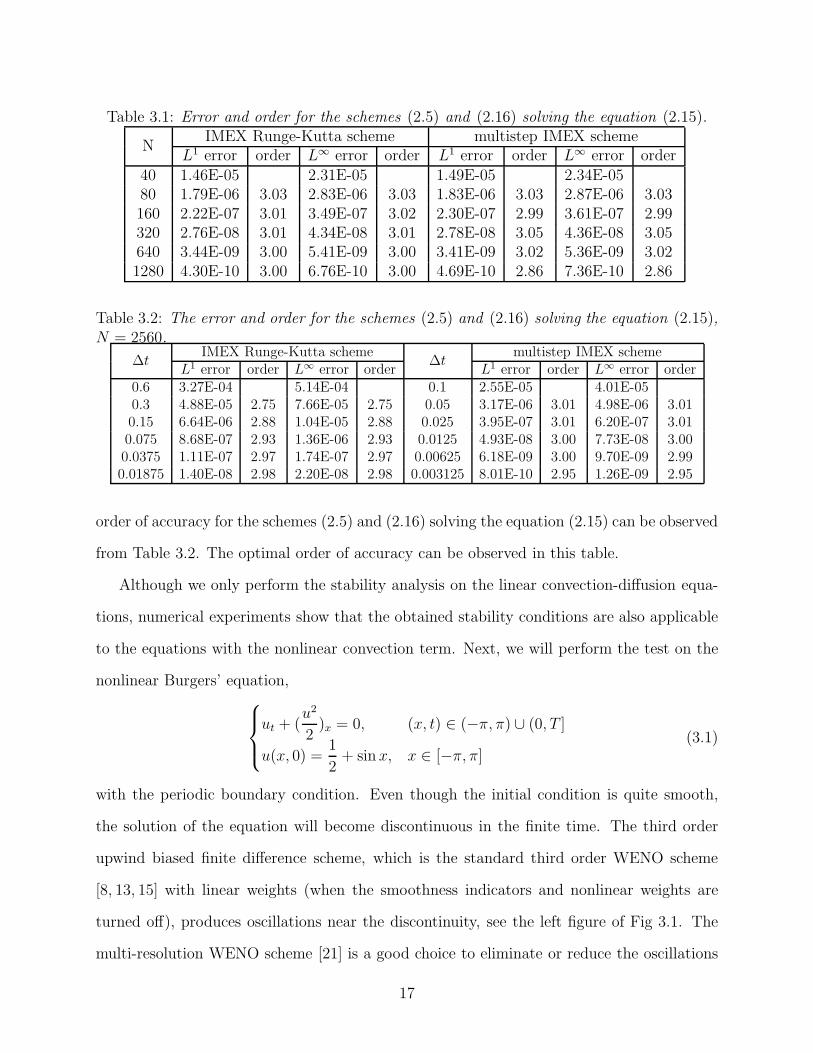
Table 3.1: Error and order for the schemes (2.5) and (2.16) solving the equation (2.15).

NIMEX Runge-Kutta scheme multistep IMEX scheme

L1 error order L∞ error order L1 error order L∞ error order40 1.46E-05 2.31E-05 1.49E-05 2.34E-0580 1.79E-06 3.03 2.83E-06 3.03 1.83E-06 3.03 2.87E-06 3.03160 2.22E-07 3.01 3.49E-07 3.02 2.30E-07 2.99 3.61E-07 2.99320 2.76E-08 3.01 4.34E-08 3.01 2.78E-08 3.05 4.36E-08 3.05640 3.44E-09 3.00 5.41E-09 3.00 3.41E-09 3.02 5.36E-09 3.021280 4.30E-10 3.00 6.76E-10 3.00 4.69E-10 2.86 7.36E-10 2.86

Table 3.2: The error and order for the schemes (2.5) and (2.16) solving the equation (2.15),N = 2560.

∆tIMEX Runge-Kutta scheme

∆tmultistep IMEX scheme

L1 error order L∞ error order L1 error order L∞ error order0.6 3.27E-04 5.14E-04 0.1 2.55E-05 4.01E-050.3 4.88E-05 2.75 7.66E-05 2.75 0.05 3.17E-06 3.01 4.98E-06 3.010.15 6.64E-06 2.88 1.04E-05 2.88 0.025 3.95E-07 3.01 6.20E-07 3.010.075 8.68E-07 2.93 1.36E-06 2.93 0.0125 4.93E-08 3.00 7.73E-08 3.000.0375 1.11E-07 2.97 1.74E-07 2.97 0.00625 6.18E-09 3.00 9.70E-09 2.990.01875 1.40E-08 2.98 2.20E-08 2.98 0.003125 8.01E-10 2.95 1.26E-09 2.95

order of accuracy for the schemes (2.5) and (2.16) solving the equation (2.15) can be observed

from Table 3.2. The optimal order of accuracy can be observed in this table.

Although we only perform the stability analysis on the linear convection-diffusion equa-

tions, numerical experiments show that the obtained stability conditions are also applicable

to the equations with the nonlinear convection term. Next, we will perform the test on the

nonlinear Burgers’ equation,

ut + (u2

2)x = 0, (x, t) ∈ (−π, π) ∪ (0, T ]

u(x, 0) =1

2+ sin x, x ∈ [−π, π]

(3.1)

with the periodic boundary condition. Even though the initial condition is quite smooth,

the solution of the equation will become discontinuous in the finite time. The third order

upwind biased finite difference scheme, which is the standard third order WENO scheme

[8, 13, 15] with linear weights (when the smoothness indicators and nonlinear weights are

turned off), produces oscillations near the discontinuity, see the left figure of Fig 3.1. The

multi-resolution WENO scheme [21] is a good choice to eliminate or reduce the oscillations

17

Figure 3.1: The third order upwind biased scheme (left) and the third order multi-resolutionWENO scheme (right) for the Burgers’ equation. Solid line: exact solution; Circle symbol:the numerical solution at T = 1.1. N = 500.

Table 3.3: The error and order of the third order upwind biased scheme (left) and multi-resolution WENO scheme (right) coupled with the third order IMEX Runge-Kutta time dis-cretization solving the equation (3.1). The time step is ∆t = 0.6∆x.

Nthe upwind biased scheme the multi-resolution WENO scheme


near the discontinuity, see the right figure of Fig 3.1.

For the Burgers’ equation, we consider both the third order upwind biased scheme and

the third order multi-resolution WENO scheme for the spatial discretization. In order to

ensure correct upwind biasing and stability, a simple Lax-Friedrichs flux splitting [16] is used.

We take ∆t = 0.6∆x for the scheme with the IMEX Runge-Kutta time discretization and

take ∆t = 0.1∆x for the scheme with the multistep IMEX time discretization. Tables 3.3

and 3.4 are the L1 and L∞ error and order of accuracy for the above mentioned schemes.

We compute the solution up to T = 0.5 in the test, when the solution is still smooth. The

optimal order of accuracy can be observed from both tables.

18

Table 3.4: The error and order of the third order upwind biased scheme (left) and multi-resolution WENO scheme (right) coupled with the third order multistep IMEX time dis-cretization solving the equation (3.1). The time step is ∆t = 0.1∆x.

Nthe upwind biased scheme the multi-resolution WENO scheme


Table 3.5: The error and order for the schemes (2.5) and (2.16) solving the equation (3.2).

NIMEX Runge-Kutta multistep IMEX


Finally, we consider the viscous Burgers’ equation [17] with a source term

ut + (u2

2)x = duxx + g(x, t), (x, t) ∈ (−π, π) ∪ (0, T ]

u(x, 0) = sin x, x ∈ [−π, π](3.2)

The source term is g(x, t) = 12e−2dt sin(2x), and the exact solution is u(x, t) = e−dt sin(x). In

order to ensure correct upwind biasing and stability, a simple Lax-Friedrichs flux splitting

is used for the convection term. For the third order IMEX Runge-Kutta finite difference

scheme (2.5) and the third order multistep IMEX finite difference scheme (2.16), we take

the time step ∆t = 0.6∆x and ∆t = 0.1∆x, respectively. Then we can again clearly observe

the designed order of accuracy for the schemes solving the equation (3.2) in Table 3.5.

19

4 The IMEX finite difference schemes for the convection-

dispersion equations

In this section, we will extend our work in Section 2 to the linear convection-dispersion

equation{

ut + ux + duxxx = 0, (x, t) ∈ (a, b) ∪ (0, T ]

u(x, 0) = u0(x), x ∈ [a, b](4.1)

with periodic boundary condition, where the dispersion coefficient d ≥ 0 is a constant. In

this section, we will focus our attention on the stability analysis for the third order IMEX

Runge-Kutta method [17], the third order additive Runge-Kutta method [11] and the second

order multistep IMEX method [18] coupled with certain high order finite difference spatial

discretization respectively. Numerical experiments are also given to demonstrate the stability

results given by the analysis.

4.1 The spatial discretization

In this subsection, we present the spatial discretization of (4.1). We adopt the third order

upwind biased finite difference scheme, which is a prototype of the third order WENO scheme

to discretize the convection term, and the third order one-point upwind biased scheme to

discretize the dispersion term. Then we can get the following semidiscrete scheme

du

dt

∣

∣

∣

∣

x=xi

= L(t, u)i +N(t, u)i (4.2)

where L(t, u)i arises from the spatial discretization of the dispersion term

L(t, u)i = −d−ui+3 + 7ui+2 − 14ui+1 + 10ui − ui−1 − ui−2

4∆x3(4.3)

and N(t, u)i is derived from the spatial discretization of the convection term. The specific

formula for N(t, u)i is given by (2.3).

4.2 The temporal discretization

In this subsection, we consider the fully discrete schemes for the ODE system (4.1). Both

Runge-Kutta and multistep IMEX time-marching methods are considered. For a detailed

20

introduction to IMEX time-marching methods, we refer to [14, 17, 18].

4.2.1 The third order IMEX Runge-Kutta finite difference scheme

We use the third order IMEX Runge-Kutta method [17] to fully discretize the above semidis-

crete scheme (4.2) and obtain

u(1) = un (4.4)

u(2) = un + γ∆t(

L(tn2 , u(2)) +N(tn1 , u(1))

)

u(3) = un +1− γ

2∆tL(tn2 , u(2)) + γ∆tL(tn3 , u(3))+

(1 + γ

2− α1

)

∆tN(tn1 , u(1)) + α1∆tN(tn2 , u

(2))

u(4) = un +∆t

(

β1L(tn2 , u(2)) + β2L(tn3 , u(3)) + γL(tn4 , u(4))

)

+

∆t

(

(1− α2)N(tn2 , u(2)) + α2N(tn3 , u

(3))

)

un+1 = un +∆t

(

β1L(tn2 , u(2)) + β2L(tn3 , u(3)) + γL(tn4 , u(4))

)

+

∆t

(

(1− α2)N(tn2 , u(2)) + α2N(tn3 , u

(3))

)

where u(s), s = 1, ..., 4 approximates u(tn+cs∆t), {cs}4s=1 = {0, γ, 1+γ

2, 1} and tns = tn+cs∆t.

γ ≈ 0.435866521508459, β1 = −32γ2 + 4γ − 1

4and β2 =

32γ2 − 5γ + 5

4. The parameter α1 is

chosen as −0.35 and α2 =1

3−2γ2

−2β2α1γ

γ(1−γ)[17].

4.2.2 The third order additive Runge-Kutta finite difference scheme

We use the third order additive Runge-Kutta method [11] to fully discretize the semidiscrete

scheme (4.2) and obtain

u(1) = un

u(i) = un +∆t

i∑

j=1

aijL(tnj , u(j)) + ∆t

i−1∑

j=1

aijN(tnj , u(j))

un+1 = un +∆t4

∑

j=1

bjL(tnj , u(j)) + ∆t4

∑

j=1

bjN(tnj , u(j))

, 2 ≤ i ≤ 4 (4.5)

21

where tni = tn + ci∆t, u(i) approximates u(tn + ci∆t) and {ci}4i=1 = {0, γ, 35 , 1}. The Butcher

coefficients aij, aij , bj , and bj are given in the following tabular data.

aij

0 0 0 0γ γ 0 0

274623878971910658868560708

−6401674452376845629431997

γ 014712663995797840856788654

−44824441678587529755066697

1126623926642811593286722821

γ

bi275625567132712835298489170

−1077155257357522201958757719

924758926504710645013368117

21932090470915459859503100

(4.6)

aij

0 0 0 02γ 0 0 0

553582888582510492691773637

78802234243710882634858940

0 0648598928062916251701735622

−42462668470899704473918619

1075544844929210357097424841

0

bi14712663995797840856788654

−44824441678587529755066697

1126623926642811593286722821

γ

(4.7)

The tabular data (4.6) list aij and bj , with the four rows from top to bottom corresponding

to i = 1, 2, 3, 4, and the columns from left to right corresponding to j = 1, 2, 3, 4 respectively.

Similarly, the tabular data (4.7) list aij and bj . In (4.6) and (4.7), the value of γ is set as

17677322059034055673282236

.

The additive Runge-Kutta method is a combination of the traditional explicit Runge-

Kutta method and an L-stable, stiffly-accurate, singly diagonally implicit Runge-Kutta

method. Compared with the IMEX Runge-Kutta finite difference scheme (4.4) of the

same order which has the advantage of simplicity, the additive Runge-Kutta finite differ-

ence scheme exhibits excellent stability in the existence of stiffness [14].

4.2.3 The second order multistep IMEX finite difference scheme

Because no multistep method of order greater than 2 can be A-stable [7], we will consider

the second order multistep IMEX time-marching method [18] with an A-stable trapezoidal

rule for the implicit part in this paper. The finite difference scheme is in the form

un+1i − un

i =∆t

(

3

2N(tn, un)i −

1

2N(tn−1, un)i

)

+

∆t

(

3

4L(tn+1, un+1)i +

1

4L(tn−1, un−1)i

) (4.8)

where N(t, u)i stems from the spatial discretization of the convection term and L(t, u)i arises

from the spatial discretization of the dispersion term. The formulas for N(t, u)i and L(t, u)i

22

Table 4.1: The Courant number c.scheme c(4.4) 1.3599(4.5) 2.03(4.8) 0.58

are specified in (2.3) and (4.3), respectively. In the following subsection, we would like to

analyze the stability of the above schemes.

4.3 Stability analysis

In [5], some IMEX Runge-Kutta methods coupled with the finite volume spatial discretiza-

tion are shown to be stable for the KdV equation under the standard CFL condition

∆t ≤ c∆x. For the IMEX schemes (4.4), (4.5), (4.8) coupled with finite difference spa-

tial discretizations solving the linear convection-dispersion equation, in which we treat the

dispersion term implicitly and the convection term explicitly, we can reasonably expect to

obtain similar stability. Because of the algebraic complexity, we will proceed in the similar

way as that in Section 2.1.1 to get the values of c. When the period is 2π and d = 0, Table

4.1 lists the maximum Courant number c which can guarantee the stability. We also find

that when d > 0, c may not be the optimal Courant number in the sense that, if we take

∆t = (c + 0.01)∆x, the norm of the amplification factor may not be greater than 1 (or the

roots of the characteristic equation may not lie outside the complex unit disk), but we can

ensure that |G| ≤ 1 (or (2.22)) holds if ∆t ≤ c∆x for any d.

In order to further verify whether the above listed c can ensure the numerical stability

of the schemes, we consider the following equation{

ut + ux + duxxx = 0, (x, t) ∈ (−π, π) ∪ (0, T ]

u(x, 0) = sin(x), x ∈ [−π, π](4.9)

with periodic boundary condition. The exact solution is u(x, t) = sin(

x − (1 − d)t)

. Since

the second order multistep IMEX finite difference scheme (4.8) is not self-starting, we adopt

the third order IMEX Runge-Kutta finite difference scheme (4.4) to compute the solution

at the first time level. In the tests, we take the time step ∆t as (c − 0.01)∆x, c∆x and

23

Table 4.2: The error of the scheme (4.4) for solving the equation (4.9) with the differenttime step.

d ∆t Nc T L1 error L∞ error

d=01.3499∆x

40 100000.5370 0.8446

1.3599∆x 0.5390 0.84711.3699∆x 3.88E+217 6.20E+217

d=0.0011.3499∆x

40 1000000.6325 0.9996

1.3599∆x 0.6325 0.99961.3699∆x 0.6325 0.9996

d=0.011.3499∆x

40 1000000.6420 1

1.3599∆x 0.6420 11.3699∆x 0.6420 1

d=0.051.3499∆x

40 1000000.6451 0.9996

1.3599∆x 0.6451 0.99961.3699∆x 0.6451 0.9996

(c+0.01)∆x, respectively. Tables 4.2, 4.3 and 4.4 show that when d = 0, the error will blow

up if we take ∆t = (c + 0.01)∆x, but is tolerable under the condition ∆t ≤ c∆x. When

d 6= 0, the L1 and L∞ error is bounded as shown in these three tables.

In general, these three schemes are stable under the standard CFL condition. Besides, it

is worth noting that the Runge-Kutta type IMEX finite difference schemes (4.4), (4.5) admit

larger time step than the multistep IMEX fully discrete scheme (4.8), and the additive Runge-

Kutta finite difference scheme (4.4) admits larger time step than the IMEX Runge-Kutta

finite difference scheme (4.5).

5 Numerical experiments

In this section, we provide a few numerical examples, including the linear and nonlinear

convection-dispersion problems, to illustrate stability condition and the error accuracy for the

third order IMEX Runge-Kutta scheme finite difference (4.4), the third order additive Runge-

Kutta finite difference scheme (4.5) and the second order multistep IMEX finite difference

scheme (4.8) respectively. In order to implement the scheme (4.8), we use the self-closed

scheme (4.4) to compute the solution at the first time level.

Consider the linear convection-dispersion equation (4.9). We take d = 0.5, and the final

24

Table 4.3: The error of the scheme (4.5) for solving the equation (4.9) with the differenttime step.

d ∆t Nc T L1 error L∞ error

d=02.02∆x

40 100000.6281 0.9993

2.03∆x 0.6281 0.99932.04∆x 2.16E+51 3.21E+51

d=0.0012.02∆x

40 1000000.6325 0.9996

2.03∆x 0.6325 0.99962.04∆x 0.6325 0.9996

d=0.012.02∆x

40 1000000.642 1

2.03∆x 0.642 12.04∆x 0.642 1

d=0.052.02∆x

40 1000000.6451 0.9996

2.03∆x 0.6451 0.99962.04∆x 0.6451 0.9996

Table 4.4: The error of the scheme (4.8) for solving (4.9) with the different time step.d ∆t Nc T L1 error L∞ error

d=00.57∆x

40 10001.1745 1.8248

0.58∆x 1.1651 1.80860.59∆x 3.45E+82 5.35E+82

d=0.0010.57∆x

40 1000000.6325 0.9996

0.58∆x 0.6325 0.99960.59∆x 0.6325 0.9996

d=0.010.57∆x

40 1000000.642 1

0.58∆x 0.642 10.59∆x 0.642 1

d=0.050.57∆x

40 1000000.6451 0.9996

0.58∆x 0.6451 0.99960.59∆x 0.6451 0.9996

25

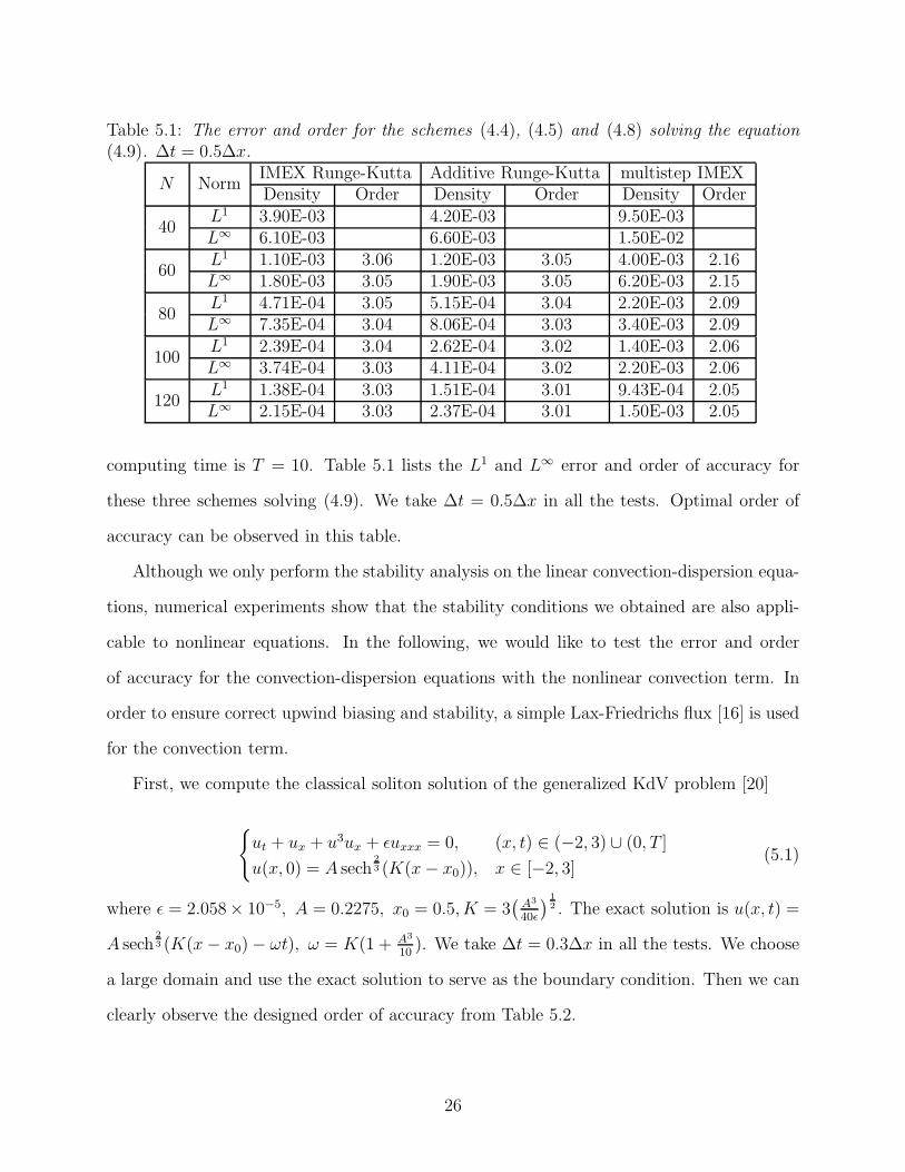
Table 5.1: The error and order for the schemes (4.4), (4.5) and (4.8) solving the equation(4.9). ∆t = 0.5∆x.

N NormIMEX Runge-Kutta Additive Runge-Kutta multistep IMEXDensity Order Density Order Density Order

40L1 3.90E-03 4.20E-03 9.50E-03L∞ 6.10E-03 6.60E-03 1.50E-02

60L1 1.10E-03 3.06 1.20E-03 3.05 4.00E-03 2.16L∞ 1.80E-03 3.05 1.90E-03 3.05 6.20E-03 2.15

80L1 4.71E-04 3.05 5.15E-04 3.04 2.20E-03 2.09L∞ 7.35E-04 3.04 8.06E-04 3.03 3.40E-03 2.09

100L1 2.39E-04 3.04 2.62E-04 3.02 1.40E-03 2.06L∞ 3.74E-04 3.03 4.11E-04 3.02 2.20E-03 2.06

120L1 1.38E-04 3.03 1.51E-04 3.01 9.43E-04 2.05L∞ 2.15E-04 3.03 2.37E-04 3.01 1.50E-03 2.05

computing time is T = 10. Table 5.1 lists the L1 and L∞ error and order of accuracy for

these three schemes solving (4.9). We take ∆t = 0.5∆x in all the tests. Optimal order of

accuracy can be observed in this table.

Although we only perform the stability analysis on the linear convection-dispersion equa-

tions, numerical experiments show that the stability conditions we obtained are also appli-

cable to nonlinear equations. In the following, we would like to test the error and order

of accuracy for the convection-dispersion equations with the nonlinear convection term. In

order to ensure correct upwind biasing and stability, a simple Lax-Friedrichs flux [16] is used

for the convection term.

First, we compute the classical soliton solution of the generalized KdV problem [20]

{

ut + ux + u3ux + ǫuxxx = 0, (x, t) ∈ (−2, 3) ∪ (0, T ]

u(x, 0) = A sech2

3 (K(x− x0)), x ∈ [−2, 3](5.1)

where ǫ = 2.058× 10−5, A = 0.2275, x0 = 0.5, K = 3(

A3

40ǫ

)1

2 . The exact solution is u(x, t) =

A sech2

3 (K(x− x0)− ωt), ω = K(1 + A3

10). We take ∆t = 0.3∆x in all the tests. We choose

a large domain and use the exact solution to serve as the boundary condition. Then we can

clearly observe the designed order of accuracy from Table 5.2.

26



80L1 1.20E-03 1.20E-03 1.10E-03L∞ 1.97E-02 1.98E-02 2.11E-02

160L1 2.49E-04 2.23 2.52E-04 2.23 2.63E-04 2.07L∞ 6.50E-03 1.60 6.50E-03 1.60 7.00E-03 1.59

320L1 3.76E-05 2.73 3.80E-05 2.73 5.88E-05 2.16L∞ 1.30E-03 2.31 1.30E-03 2.30 1.70E-03 2.02

640L1 5.03E-06 2.90 5.09E-06 2.90 1.36E-05 2.12L∞ 1.91E-04 2.77 1.94E-04 2.77 3.88E-04 2.15

1280L1 6.35E-07 2.98 6.43E-07 2.98 3.34E-06 2.02L∞ 2.45E-05 2.97 2.47E-05 2.97 9.49E-05 2.03



80L1 1.60E-02 1.65E-02 1.75E-02L∞ 1.18E-01 1.24E-01 1.45E-01

160L1 2.50E-03 2.68 2.60E-03 2.64 3.90E-03 2.18L∞ 1.79E-02 2.72 1.93E-02 2.67 3.05E-02 2.25

320L1 3.23E-04 2.95 3.57E-04 2.89 9.21E-04 2.07L∞ 2.30E-03 2.95 2.60E-03 2.88 6.90E-03 2.15

640L1 4.08E-05 2.99 4.80E-05 2.89 2.31E-04 1.99L∞ 2.88E-04 3.01 3.64E-04 2.85 1.70E-03 1.98

1280L1 5.11E-06 3.00 6.97E-06 2.78 5.84E-05 1.98L∞ 3.56E-05 3.01 5.39E-05 2.76 4.30E-04 2.02

Next, we compute the classical soliton solution of the KdV problem [20]

{

ut − 3(u2)x + uxxx = 0, (x, t) ∈ (−10, 12) ∪ (0, T ]

u(x, 0) = −2 sech2(x), x ∈ [−10, 12](5.2)

The exact solution is u(x, t) = −2 sech2(x− 4t). We take ∆t = 0.1∆x in all the tests. Table

5.3 gives the L1 and L∞ error and order of accuracy at T = 0.5 using the exact solution to

serve as the boundary condition. The optimal order of accuracy can be observed from this

table.

27

Table 5.4: The error and order for the schemes (4.4), (4.5) and (4.8) solving the equation(5.3). The time step is ∆t = 0.1∆x.


160L1 5.36E-04 5.36E-04 6.40E-04L∞ 1.29E-02 1.29E-02 1.88E-02

320L1 9.18E-05 2.55 9.18E-05 2.55 1.15E-04 2.48L∞ 2.00E-03 2.68 2.00E-03 2.67 3.70E-03 2.34

640L1 1.27E-05 2.85 1.27E-05 2.85 2.28E-05 2.33L∞ 2.65E-04 2.92 2.66E-04 2.92 6.75E-04 2.46

1280L1 1.64E-06 2.96 1.64E-06 2.95 4.96E-06 2.20L∞ 3.35E-05 2.99 3.35E-05 2.99 1.18E-04 2.51

2560L1 2.07E-07 2.99 2.07E-07 2.99 1.23E-06 2.01L∞ 4.20E-06 3.00 4.21E-06 2.99 2.63E-05 2.17

Finally, we consider the soliton solution of the mKdV problem{

ut + 6u2ux + uxxx = 0, (x, t) ∈ (−40, 40) ∪ (0, T ]

u(x, 0) =√c sech(

√cx), x ∈ [−40, 40]

(5.3)

The exact solution is u(x, t) =√c sech

(√c(x − ct)

)

. Here, we take c = 12. We take ∆t =

0.1∆x in all the tests. Table 5.4 gives the L1 and L∞ error and order of accuracy at T = 0.5

using the exact solution to serve as the boundary conditions. We can clearly observe the

designed order of accuracy from this table.

6 Concluding remarks

We have considered some carefully chosen IMEX time marching methods coupled with high

order finite difference spatial discretization for solving the linear convection-diffusion and the

convection-dispersion equations with periodic boundary conditions. By the aid of the Fourier

method, a procedure in Matlab is used to get the time step restriction of the schemes. For the

convection-diffusion equations, the result shows that the IMEX finite difference schemes are

stable under the condition ∆t ≤ max{τ0, c∆x}, in which τ0 is a positive constant proportional

to the diffusion coefficient and c is the Courant number. For the convection-dispersion

equations, the result shows that the IMEX finite difference schemes are stable under the

standard CFL condition ∆t ≤ c∆x. In addition, we can find that the Runge-Kutta type

28

IMEX finite difference schemes admit larger time step than the multistep type IMEX finite

difference schemes. The numerical tests verify the designed order of accuracy for these IMEX

finite difference schemes under the stability condition.

References

[1] U. M. Ascher, S. J. Ruuth and B. T. R. Wetton, Implicit-explicit methods for time-

dependent partial differential equations, SIAM Journal on Numerical Analysis, 32, 1995,

797-823.

[2] U. M. Ascher, S. J. Ruuth and R. J. Spiteri, Implicit-explicit Runge-Kutta methods for

time-dependent partial differential equations, Applied Numerical Mathematics, 25, 1997,

151-167.

[3] J. Bruder, Linearly-implicit Runge-Kutta methods based on implicit Runge-Kutta meth-

ods, Applied Numerical Mathematics, 13, 1993, 33-40.

[4] M. P. Calvo, J. D. Frutos and J. Novo, Linearly implicit Runge-Kutta methods for

advection-reaction-diffusion equations, Applied Numerical Mathematics, 37, 2001, 535-

549.

[5] D. Dutykh, T. Katsaounis and D. Mitsotakis, Finite volume methods for unidirectional

dispersive wave models, International Journal for Numerical Methods in Fluids, 71,

2013, 717-736.

[6] B. Fornberg and T. A. Driscoll, A fast spectral algorithm for nonlinear wave equations

with linear dispersion, Journal of Computational Physics, 155, 1999, 456-467.

[7] J. Frank, W. Hundsdorfer and J. G. Verwer, On the stability of implicit-explicit linear

multistep methods, Applied Numerical Mathematics, 25, 1997, 193-205.

[8] G. A. Gerolymos, D. Senechal and I. Vallet, Very-high-order WENO schemes, Journal

of Computational Physics, 228, 2009, 8481-8524.

29

[9] S. Gottlieb, C.-W. Shu and E. Tadmor, Strong stability-preserving high-order time dis-

cretization methods, SIAM Review, 43, 2001, 89-112.

[10] S. Gottlieb and C. Wang, Stability and convergence analysis of fully discrete Fourier

collocation spectral method for 3-D viscous Burgers’ equation, Journal of Scientific Com-

puting, 53, 2012, 102-128.

[11] R. Guo and Y. Xu, Fast solver for the local discontinuous Galerkin discretization of the

KdV type equations, Journal of Scientific Computing, 58, 2014, 380-408.

[12] A. C. Hindmarsh, P. M. Gresho and D. F. Griffiths, The stability of explicit euler

time-integration for certain finite difference approximations of the multi-dimensional

advection-diffusion equation, International Journal for Numerical Methods in Fluids, 4,

1984, 853-897.

[13] G. S. Jiang and C.-W. Shu, Efficient implementation of weighted ENO schemes, Journal


[14] C. A. Kennedy and M. H. Carpenter, Additive Runge-Kutta schemes for convection-

diffusion-reaction equations, Applied Numerical Mathematics, 44, 2003, 139-181.

[15] X. D. Liu, S. Osher and T. Chan, Weighted essentially non-oscillatory scheme, Journal


[16] C.-W. Shu, Essentially non-oscillatory and weighted essentially non-oscillatory schemes

for hyperbolic conservation laws, in Advanced Numerical Approximation of Nonlinear

Hyperbolic Equations, B. Cockburn, C. Johnson, C.-W. Shu and E. Tadmor (Editor:

A. Quarteroni), Lecture Notes in Mathematics, volume 1697, Springer, Berlin, 1998,

pp.325-432.

30

[17] H. J. Wang, C.-W. Shu and Q. Zhang, Stability and error estimates of local discontinuous

Galerkin methods with implicit-explicit time-marching for advection-diffusion problems,

SIAM Journal on Numerical Analysis, 53, 2015, 206-227.

[18] H. J. Wang, C.-W. Shu and Q. Zhang, Stability analysis and error estimates of lo-

cal discontinuous Galerkin methods with implicit-explicit time-marching for nonlinear

convection-diffusion problems, Applied Mathematics and Computation, 272, 2016, 237-

258.

[19] H. J. Wang, Q. Zhang and C.-W. Shu, Implicit-explicit local discontinuous Galerkin

methods with generalized alternating numerical fluxes convection-diffusion problems,

Journal of Scientific Computing, 81, 2019, 1-35.

[20] J. Yan and C.-W. Shu, A local discontinuous Galerkin method for KdV type equations,

SIAM Journal on Numerical Analysis, 40, 2002, 769-791.

[21] J. Zhu and C.-W. Shu, A new type of multi-resolution WENO schemes with increasingly

higher order of accuracy, Journal of Computational Physics, 375, 2018, 659-683.

31

Appendix A

1. The amplification factor G of the third order IMEX Runge-Kutta finite

difference scheme (2.5) solving the convection-diffusion equation.

Substituting the Fourier modes unj = vneIkxj , I2 = −1 into the first four difference

equations in (2.5) yields

v(2) = M2vn v(3) = M3v

n v(4) = M4vn

where

M2 =1 +∆tGN a211−∆tGLa22

M3 =1 +∆tGN

(

a31 + a32M2

)

+∆tGLa32M2

1−∆tGLa33

M4 =1 +∆tGN

(

a41 + a42M2 + a43M3

)

+∆tGL(

a42M2 + a43M3

)

1−∆tGLa44

GL =d

12∆x2

(

2 cos 2ξ − 32 cos ξ + 30)

GN = − 1

∆x

(1

2+

1

3cos ξ +

1

3I sin ξ − cos ξ + I sin ξ +

1

6cos 2ξ − 1

6I sin 2ξ

)

with ξ given by ξ = k∆x. The Butcher coefficients asj, asj, bj , bj , s = 1, ..., 4; j = 1, ..., 4 are

specified in (2.6). Substitute the above formula into the last term of (2.5), and we can get

the amplification factor G after a simple arithmetic operation.

G = 1 +∆tGN(

b1 + b2M2 + b3M3 + b4M4

)

+∆tGL(

b1 + b2M2 + b3M3 + b4M4

)

2. The coefficients of the characteristic equation (2.20).

a1 =1 + 23

12∆tGN

1− 23∆tGL

a2 =−4

3∆tGN + 5

12∆tGL

1− 23∆tGL

a3 =512∆tGN

1− 23∆tGL

a4 =− 1

12∆tGL

1− 23∆tGL

32

Appendix B

For the IMEX Runge-Kutta finite difference scheme (2.5), the Courant number c and the

maximum time step τ0 have been obtained numerically using the Matlab code. Note that

the stability analysis described in Section 2.1.1 is carried out by considering whether the

condition |G| ≤ 1 is satisfied. Taking the maximum time step τ0 as an example, the algorithm

developed for the scheme is presented below.

Algorithm 1 : Numerical stability analysis of the third order IMEX Runge-Kutta finite

difference scheme (2.5) for solving the linear convection-diffusion equation with periodic

boundary condition.

Input: d: diffusion coefficient

Output: τ0: the maximum time step

1: function Mainfunction(d)

2: τ0 ← 0

3: bool1 ← 1

4: N ← 105

5: ∆x← 2πN

6: while (1) do

7: ∆t← τ0

8: for k = 1→ N do

9: compute |G|, where G is a function of d,∆t,∆x, k

10: if |G| > 1 then

11: bool1 ← 0

12: break;

13: end if

14: end for

15: if bool1 6= 0 then

16: τ0 ← τ0 + 0.01

33

17: else

18: break;

19: end if

20: end while

21: return τ0

22: end function

34

stability of high order ﬁnite diﬀerence schemes with

Documents