stability and sensitivity analysis in optimal control of ... · pdf filepreface the topic of...

Stability and Sensitivity Analysisin Optimal Control

of Partial Differential Equations

Dr. rer. nat. Roland Griesse

Cumulative Habilitation Thesis

Faculty of Natural Sciences

Karl-Franzens University Graz

October 2007

Contents

Preface 3

Chapter 1. Stability and Sensitivity Analysis 71. Lipschitz Stability of Solutions for Elliptic Optimal Control Problems with

Pointwise State Constraints 122. Lipschitz Stability of Solutions for Elliptic Optimal Control Problems with

Pointwise Mixed Control-State Constraints 293. Sensitivity Analysis for Optimal Control Problems Involving the

Navier-Stokes Equations 454. Sensitivity Analysis for Optimal Boundary Control Problems of a 3D

Reaction-Diffusion System 62

Chapter 2. Numerical Methods and Applications 815. Local Quadratic Convergence of SQP for Elliptic Optimal Control

Problems with Mixed Control-State Constraints 826. Update Strategies for Perturbed Nonsmooth Equations 1027. Quantitative Stability Analysis of Optimal Solutions in PDE-Constrained

Optimization 1248. Numerical Sensitivity Analysis for the Quantity of Interest in PDE-

Constrained Optimization 1459. On the Interplay Between Interior Point Approximation and Parametric

Sensitivities in Optimal Control 174

Bibliography 195

Preface

The topic of this thesis is stability and sensitivity analysis in optimal control of partialdifferential equations. Stability refers to the continuous behavior of optimal solutionsunder perturbations of the problem data, while sensitivity indicates a differentiabledependence.

This thesis is divided into two chapters. Chapter 1 provides a short overview over thetopic and its theoretical foundations. The individual sections give an introduction tothe author’s contributions concerning new stability and sensitivity results for severalproblem classes, in particular optimal control problems with state constraints (Sec-tion 1) and mixed control-state constraints (Section 2), as well as problems involvingthe Navier-Stokes equations (Section 3) and boundary control problems for a system ofcoupled reaction-diffusion equations (Section 4). Chapter 1 is based on the followingpublications.

1. R. Griesse: Lipschitz Stability of Solutions to Some State-Constrained EllipticOptimal Control Problems, Journal of Analysis and its Applications, 25(4),p.435–444, 2006

2. W. Alt, R. Griesse, N. Metla and A. Rosch: Lipschitz Stability for EllipticOptimal Control Problems with Mixed Control-State Constraints, submittedto Applied Mathematics and Optimization, 2006

3. R. Griesse, M. Hintermuller and M. Hinze: Differential Stability of Con-trol Constrained Optimal Control Problems for the Navier-Stokes Equations,Numerical Functional Analysis and Optimization 26(7–8), p.829–850, 2005

4. R. Griesse and S. Volkwein: Parametric Sensitivity Analysis for OptimalBoundary Control of a 3D Reaction-Diffusion System, in: Large-Scale Non-linear Optimization, G. Di Pillo and M. Roma (editors), volume 83 of Non-convex Optimization and its Applications, p.127–149, Springer, Berlin, 2006

Chapter 2 addresses a number of applications based on the concepts of stability andsensitivity of infinite dimensional optimization problems, and of optimal control prob-lems in particular. The applications include the local convergence of the SQP (se-quential quadratic programming) method for optimal control problems with mixedcontrol-state constraints (Section 5), accurate update strategies for solutions of per-turbed problems (Section 6), the quantitative stability analysis of optimal solutions(Section 7), and the efficient evaluation of first and second-order sensitivity derivativesof a quantity of interest (Section 8). Finally, the relationship between the sensitivityderivatives of optimization problems in function space, and the sensitivity derivativesof their relaxations in the context of interior point methods is investigated (Section 9).Chapter 2 is based on the following publications.

5. R. Griesse, N. Metla and A. Rosch: Local Quadratic Convergence of SQPfor Elliptic Optimal Control Problems with Mixed Control-State Constraints,submitted to: ESAIM: Control, Optimisation, and Calculus of Variations,2007

4 Preface

6. R. Griesse, T. Grund and D. Wachsmuth: Update Strategies for PerturbedNonsmooth Equations, to appear in: Optimization Methods and Software,2007

7. K. Brandes and R. Griesse: Quantitative Stability Analysis of Optimal So-lutions in PDE-Constrained Optimization, Journal of Computational andApplied Mathematics, 206(2), p.809–826, 2007

8. R. Griesse and B. Vexler: Numerical Sensitivity Analysis for the Quantityof Interest in PDE-Constrained Optimization, SIAM Journal on ScientificComputing, 29(1), p.22–48, 2007

9. R. Griesse and M. Weiser: On the Interplay Between Interior Point Approx-imation and Parametric Sensitivities in Optimal Control, Journal of Mathe-matical Analysis and Applications, 337(2), p.771–793, 2008

An effort was made to use a consistent notation throughout the introductory para-graphs which link the individual papers. As a consequence, the notation used in theintroduction to each section may differ slightly from the notation used in the actualpublication. Moreover, all manuscripts have been typeset again from their LATEXsources, in order to achieve a uniform layout. In some cases, this may have led to anupdated bibliography, or a different numbering scheme.

All of the above publications were written after the completion of the author’s Ph.D.degree in February of 2003. In addition, the following publications were completed inthe same period of time.

10. R. Griesse and D. Lorenz: A Semismooth Newton Method for Tikhonov Func-tionals with Sparsity Constraints, submitted, 2007

11. R. Griesse and K. Kunisch: Optimal Control for a Stationary MHD System inVelocity-Current Formulation, SIAM Journal on Control and Optimization,45(5), p.1822–1845, 2006

12. A. Borzı and R. Griesse: Distributed Optimal Control of Lambda-OmegaSystems, Journal of Numerical Mathematics 14(1), p.17–40, 2006

13. A. Borzı and R. Griesse: Experiences with a Space-Time Multigrid Method forthe Optimal Control of a Chemical Turbulence Model, International Journalfor Numerical Methods in Fluids 47(8–9), p.879–885, 2005

14. R. Griesse and S. Volkwein: A Primal-Dual Active Set Strategy for OptimalBoundary Control of a Reaction-Diffusion System, SIAM Journal of Controland Optimization 44(2), p.467–494, 2005

15. R. Griesse and A.J. Meir: Modeling of an MHD Free Surface Problem Arisingin CZ Crystal Growth, submitted, 2007

16. J.C. de los Reyes and R. Griesse: State-Constrained Optimal Control of theStationary Navier-Stokes Equations, submitted, 2006

17. R. Griesse, A.J. Meir and K. Kunisch: Control Issues in Magnetohydrody-namics, in: Optimal Control of Free Boundaries, Mathematisches Forschungsin-stitut Oberwolfach, Report No. 8/2007, p.20–23, 2007

18. R. Griesse and A.J. Meir: Modeling of an MHD Free Surface Problem Aris-ing in CZ Crystal Growth, in: Proceedings of the 5th IMACS Symposium onMathematical Modelling (5th MATHMOD), I. Troch, F. Breitenecker (edi-tors), ARGESIM Report 30, Vienna, 2006

19. R. Griesse and K. Kunisch: Optimal Control in Magnetohydrodynamics, in:Optimal Control of Coupled Systems of PDE, Mathematisches Forschungsin-stitut Oberwolfach, Report No. 18/2005, p.1011–1014, 2005

5

20. R. Griesse and A. Walther: Towards Matrix-Free AD-Based Precondition-ing of KKT Systems in PDE-Constrained Optimization, Proceedings of theGAMM 2005 Annual Scientific Meeting, PAMM 5(1), p.47–50, 2005

21. R. Griesse and S. Volkwein: A Semi-Smooth Newton Method for OptimalBoundary Control of a Nonlinear Reaction-Diffusion System, Proceedings ofthe Sixteenth International Symposium on Mathematical Theory of Networksand Systems (MTNS), Leuven, Belgium, 2004

A complete and updated list of publications can be found online at

http://www.ricam.oeaw.ac.at/people/page/griesse/publications.html

Acknowledgment. The publications which form the basis of this thesis werewritten during my postdoctoral appointments at Karl-Franzens University of Graz(supported by the SFB 003 Optimization and Control), and at the Johann RadonInstitute for Computational and Applied Mathematics (RICAM), Austrian Academyof Sciences, in Linz. I would like to express my gratitude to Prof. Karl Kunisch forgiving me the opportunity to work in these two tremendous environments—both sci-entifically and otherwise—, for his continuous support and many inspiring discussions.I would also like to thank Prof. Heinz Engl, director of RICAM, for the opportunityto be part of this fantastic institute. The support of several project proposals by theAustrian Science Fund (FWF) is gratefully acknowledged.

My sincere thanks go to former and current colleagues and co-workers in Graz and Linz,who contributed greatly in making the recent years very enjoyable and successful. Iwould like to mention in particular Stefan Volkwein, Georg Stadler, Juan Carlos de losReyes, Alfio Borzı, and Michael Hintermuller in Graz, and Arnd Rosch, Boris Vexler,Marco Discacciati, Nataliya Metla, Svetlana Cherednichenko, Klaus Krumbiegel, OlafBenedix, Martin Bernauer, Frank Schmidt, Sven Beuchler, Joachim Schoberl, HerbertEgger, Georg Regensburger, Martin Giese, Jorn Sass, and, of course, Annette Weihs,Florian Tischler, Doris Nikolaus, Magdalena Fuchs and Wolfgang Forsthuber in Linz.Many thanks also to all co-authors who have not yet been mentioned, for their effortand time.

Last but not least, I would like to thank Julia for her constant love and support.

Linz, October 2007

CHAPTER 1

Stability and Sensitivity Analysis

Stability and sensitivity are important concepts in continuous optimization. Stabilityrefers to the continuous dependence of an optimal solution on the problem data. Inother words, stability ensures the well-posedness of the problem. On the other hand,sensitivity information allows further quantification of the solution’s dependence onproblem data, using appropriate notions of differentiability. For a general account ofperturbation analysis for infinite-dimensional optimization problems, we refer to thebook of Bonnans and Shapiro [2000].In this chapter, we consider the notions of stability and sensitivity of optimal controlproblems involving partial differential equations (PDEs). To fix ideas, we use as anexample the following prototypical distributed optimal control problem for the Poissonequation, subject to perturbations δ.

(P(δ))Minimize

12‖y − yd‖2L2(Ω) +

γ

2‖u‖2L2(Ω) − (δ1, y)Ω − (δ2, u)Ω

subject to−∆y = u+ δ3 in Ω,

y = 0 on Γ.

The state y and control u are sought in H10 (Ω) and L2(Ω), respectively, and we assume

a positive control cost parameter γ > 0. We note that the system of necessary andsufficient optimality conditions associated to (P(δ)) is given by

(0.1)

−∆p+ y − yd = δ1 in Ω, p = 0 on Γ,γ u− p = δ2 in Ω,−∆y − u = δ3 in Ω, y = 0 on Γ,

where p is the adjoint state, and δ appears as a right hand side perturbation. Theunderstanding of problems of type (P(δ)) is key to the analysis of nonlinear optimalcontrol problems which depend on a general perturbation parameter π, which mayenter nonlinearly. Properties of nonlinear problems can be deduced from properties of(P(δ)) by means of an implicit function theorem, as outlined below.In addition to problem (P(δ)), we consider some variations with pointwise controlconstraints, pointwise state constraints, or pointwise mixed control-state constraints.This leads us to consider

Solve (P(δ)) s.t. ua ≤ u ≤ ub a.e. in Ω,(Pcc(δ))

Solve (P(δ)) s.t. ya ≤ y ≤ yb in Ω,(Psc(δ))

Solve (P(δ)) s.t. yc ≤ ε u+ y ≤ yd in Ω.(Pmc(δ))

The Control Constrained Case. Lipschitz stability properties of problems oftype (Pcc(δ)) were first investigated in Unger [1997] and Malanowski and Troltzsch[2000] for the elliptic case and in Malanowski and Troltzsch [1999] for the paraboliccase. We give here a brief account of their results, applied to our model problem(Pcc(δ)). Problems with pointwise state constraints and mixed control-state con-straints will be addressed in Sections 1 and 2, respectively.

8 Stability and Sensitivity Analysis

Assumption 0.1:Suppose that Ω ⊂ Rd, d ≥ 1, is a bounded Lipschitz domain and that γ > 0 andyd ∈ L2(Ω) hold.

It is well known that (Pcc(δ)) possesses a unique solution (yδ, uδ) ∈ H10 (Ω)× Uad,

Uad := u ∈ L2(Ω) : ua ≤ u ≤ ub a.e. in Ω,provided that Uad 6= ∅. The solution and the associated unique adjoint state pδ ∈H1

0 (Ω) are characterized by the following optimality system:

(0.2)

−∆pδ + yδ − yd = δ1 in Ω, pδ = 0 on Γ,−∆yδ − uδ = δ3 in Ω, yδ = 0 on Γ,

(γ uδ − pδ − δ2, u− uδ)Ω ≥ 0 for all u ∈ Uad.

We begin by reviewing a Lipschitz stability result for the solution. For related re-sults concerning optimal control of parabolic equations, we refer to Malanowski andTroltzsch [1999], Troltzsch [2000].

Theorem 0.2 (Malanowski and Troltzsch [2000]):There exists a constant L2 such that

‖yδ − yδ′‖H1(Ω) + ‖uδ − uδ′‖L2(Ω) + ‖pδ − pδ′‖H1(Ω) ≤ L2 ‖δ − δ′‖[L2(Ω)]3

holds for every δ, δ′ ∈ [L2(Ω)]3.

When the perturbations and other problem data are more regular, a stronger resultcan be obtained:

Corollary 0.3 (compare Malanowski and Troltzsch [2000]):If yd, ua, ub ∈ L∞(Ω), then there exists a constant L∞ such that

‖yδ − yδ′‖L∞ + ‖uδ − uδ′‖L∞(Ω) + ‖pδ − pδ′‖L∞(Ω) ≤ L∞ ‖δ − δ′‖[L∞(Ω)]3

holds for every δ, δ′ ∈ [L∞(Ω)]3.

Indeed, the assumption on yd, δ1 and δ3 can be relaxed depending on the regularityof the solutions of the state and adjoint PDEs, i.e., depending on the dimension of Ωand the smoothness of its boundary Γ.

Sensitivity Analysis in the Control Constrained Case. We now addressdifferentiability properties of the parameter-to-solution map

δ 7→ ξ(δ) := (ξy(δ), ξu(δ), ξp(δ)) = (yδ, uδ, pδ).

We refer to Malanowski [2002, 2003a] for the original contributions in the elliptic andparabolic cases, respectively. Due to the presence of inequality constraints, ξ is anonlinear function of the perturbation δ. We remark that the optimal control can beexpressed as

uδ := ΠUad

(pδ + δ2γ

),

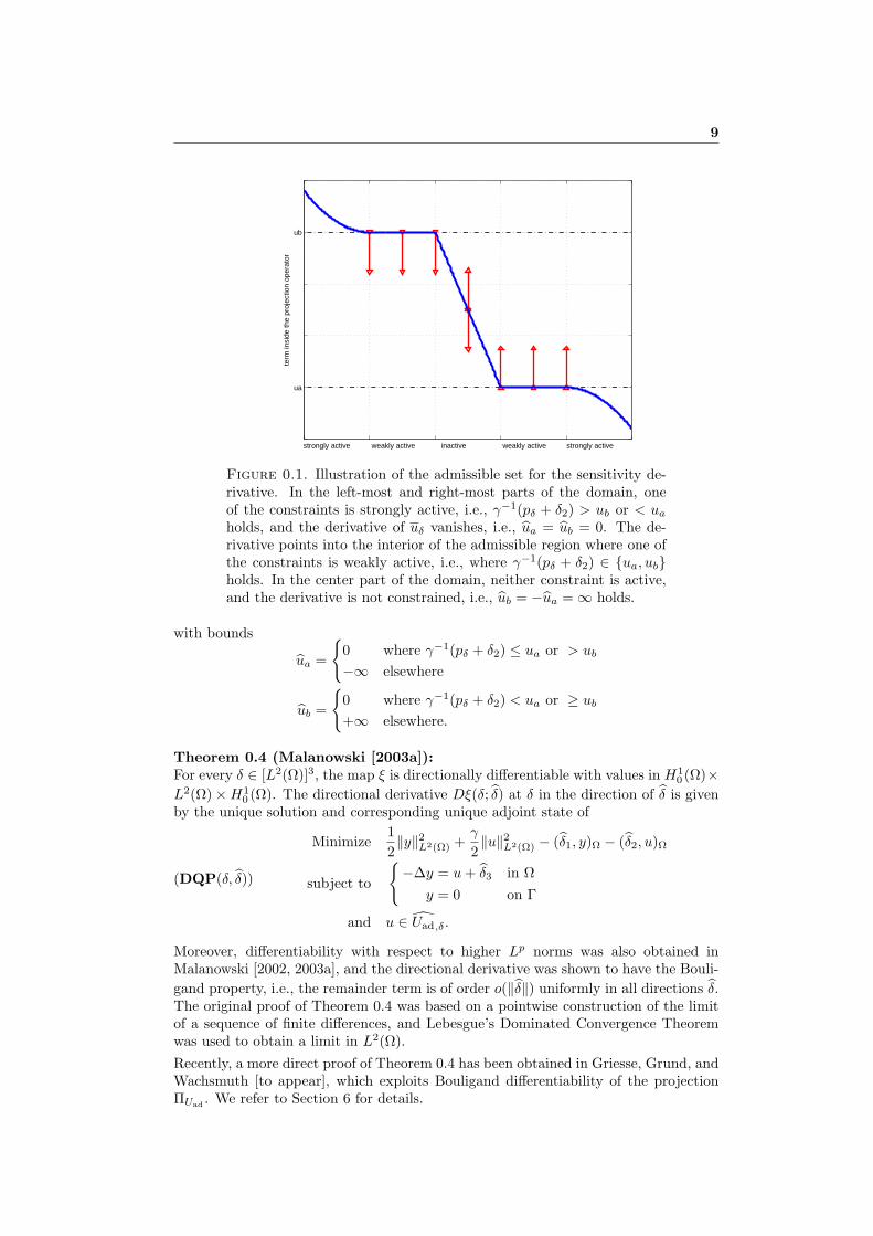
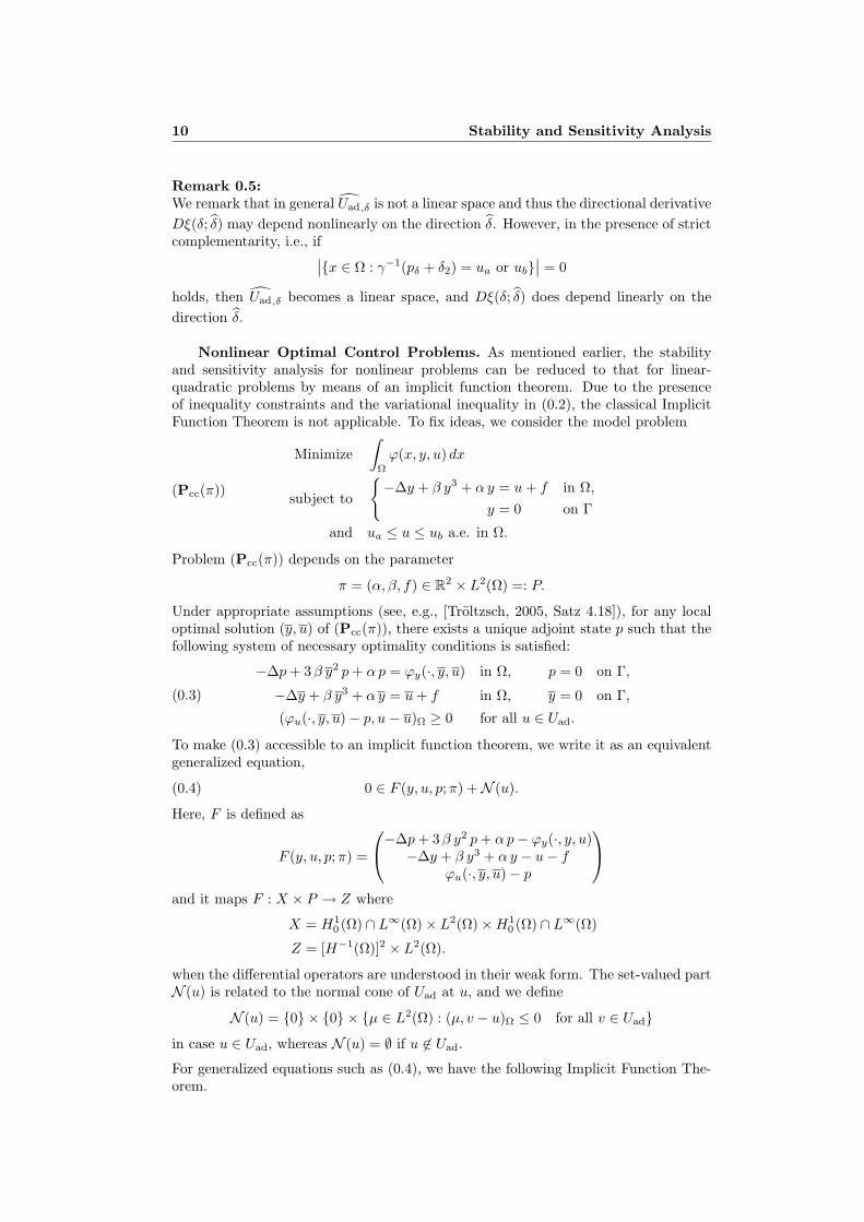
where ΠUad denotes the pointwise projection onto the set Uad. Hence the differentia-bility properties of ξ are essentially those of the projection. Naturally, the subset of Ωwhere the projection is active or strongly active will play a role, compare Figure 0.1.We define

Uad,δ := u ∈ L2(Ω) : ua ≤ u ≤ ub,

9

strongly active weakly active inactive weakly active strongly active

ua

ub

term

insi

de th

e pr

ojec

tion

oper

ator

Figure 0.1. Illustration of the admissible set for the sensitivity de-rivative. In the left-most and right-most parts of the domain, oneof the constraints is strongly active, i.e., γ−1(pδ + δ2) > ub or < uaholds, and the derivative of uδ vanishes, i.e., ua = ub = 0. The de-rivative points into the interior of the admissible region where one ofthe constraints is weakly active, i.e., where γ−1(pδ + δ2) ∈ ua, ubholds. In the center part of the domain, neither constraint is active,and the derivative is not constrained, i.e., ub = −ua =∞ holds.

with bounds

ua =

0 where γ−1(pδ + δ2) ≤ ua or > ub

−∞ elsewhere

ub =

0 where γ−1(pδ + δ2) < ua or ≥ ub+∞ elsewhere.

Theorem 0.4 (Malanowski [2003a]):For every δ ∈ [L2(Ω)]3, the map ξ is directionally differentiable with values in H1

0 (Ω)×L2(Ω)×H1

0 (Ω). The directional derivative Dξ(δ; δ) at δ in the direction of δ is givenby the unique solution and corresponding unique adjoint state of

(DQP(δ, δ))

Minimize12‖y‖2L2(Ω) +

γ

2‖u‖2L2(Ω) − (δ1, y)Ω − (δ2, u)Ω

subject to

−∆y = u+ δ3 in Ω

y = 0 on Γ

and u ∈ Uad,δ.

Moreover, differentiability with respect to higher Lp norms was also obtained inMalanowski [2002, 2003a], and the directional derivative was shown to have the Bouli-gand property, i.e., the remainder term is of order o(‖δ‖) uniformly in all directions δ.The original proof of Theorem 0.4 was based on a pointwise construction of the limitof a sequence of finite differences, and Lebesgue’s Dominated Convergence Theoremwas used to obtain a limit in L2(Ω).Recently, a more direct proof of Theorem 0.4 has been obtained in Griesse, Grund, andWachsmuth [to appear], which exploits Bouligand differentiability of the projectionΠUad . We refer to Section 6 for details.


Remark 0.5:We remark that in general Uad,δ is not a linear space and thus the directional derivativeDξ(δ; δ) may depend nonlinearly on the direction δ. However, in the presence of strictcomplementarity, i.e., if∣∣x ∈ Ω : γ−1(pδ + δ2) = ua or ub

∣∣ = 0

holds, then Uad,δ becomes a linear space, and Dξ(δ; δ) does depend linearly on thedirection δ.

Nonlinear Optimal Control Problems. As mentioned earlier, the stabilityand sensitivity analysis for nonlinear problems can be reduced to that for linear-quadratic problems by means of an implicit function theorem. Due to the presenceof inequality constraints and the variational inequality in (0.2), the classical ImplicitFunction Theorem is not applicable. To fix ideas, we consider the model problem

(Pcc(π))

Minimize∫

Ω

ϕ(x, y, u) dx

subject to

−∆y + β y3 + α y = u+ f in Ω,

y = 0 on Γ

and ua ≤ u ≤ ub a.e. in Ω.

Problem (Pcc(π)) depends on the parameter

π = (α, β, f) ∈ R2 × L2(Ω) =: P.

Under appropriate assumptions (see, e.g., [Troltzsch, 2005, Satz 4.18]), for any localoptimal solution (y, u) of (Pcc(π)), there exists a unique adjoint state p such that thefollowing system of necessary optimality conditions is satisfied:

(0.3)

−∆p+ 3β y2 p+ αp = ϕy(·, y, u) in Ω, p = 0 on Γ,

−∆y + β y3 + α y = u+ f in Ω, y = 0 on Γ,

(ϕu(·, y, u)− p, u− u)Ω ≥ 0 for all u ∈ Uad.

To make (0.3) accessible to an implicit function theorem, we write it as an equivalentgeneralized equation,

(0.4) 0 ∈ F (y, u, p;π) +N (u).

Here, F is defined as

F (y, u, p;π) =

−∆p+ 3β y2 p+ αp− ϕy(·, y, u)−∆y + β y3 + α y − u− f

ϕu(·, y, u)− p

and it maps F : X × P → Z where

X = H10 (Ω) ∩ L∞(Ω)× L2(Ω)×H1

0 (Ω) ∩ L∞(Ω)

Z = [H−1(Ω)]2 × L2(Ω).

when the differential operators are understood in their weak form. The set-valued partN (u) is related to the normal cone of Uad at u, and we define

N (u) = 0 × 0 × µ ∈ L2(Ω) : (µ, v − u)Ω ≤ 0 for all v ∈ Uadin case u ∈ Uad, whereas N (u) = ∅ if u 6∈ Uad.

For generalized equations such as (0.4), we have the following Implicit Function The-orem.

11

Theorem 0.6 ([Dontchev, 1995, Theorem 2.4]):Let X be a Banach space and let P,Z be normed linear spaces. Suppose that F :X×P → Z is a function and N : X → Z is a set-valued map. Let x ∈ X be a solutionto

(0.5) 0 ∈ F (x;π) +N (x)

for π = π0, and let W be a neighborhood of 0 ∈ Z. Suppose that

(i) F is Lipschitz in π, uniformly in x at (x, π0), and F (x, ·) is directionallydifferentiable at π0 with directional derivative DπF (x, π0); δπ) for all δπ ∈ P ,

(ii) F is partially Frechet differentiable with respect to x in a neighborhood of(x, π0), and its partial derivative Fx is continuous in both x and π at (x, π0),

(iii) there exists a function ξ : W → X such that ξ(0) = x, δ ∈ F (x, π0) +Fx(x, π0)(ξ(δ)− x) +N (ξ(δ)) for all δ ∈ W, and ξ is Lipschitz continuous.

Then there exist neighborhoods U of x and V of π0 and a function

π 7→ Ξ(π) = x(π)

from V to U such that Ξ(π0) = x, Ξ(π) is a solution of (0.5) for every π ∈ V , and Ξis Lipschitz continuous.

If, in addition, X ⊃ X is a normed linear space such that

(iv) ξ :W → X is directionally (or Bouligand) differentiable at 0 with derivativeDξ(0; δ) for all δ ∈ Z,

then π 7→ Ξ(π) ∈ X is also directionally (or Bouligand) differentiable at π0 and itsderivative is given by

(0.6) DΞ(π0; δπ) = Dξ(0;−DπF ((x, π0); δπ),

for any δπ ∈ P .

Definition 0.7 (Robinson [1980]):The property (iii) is termed the strong regularity of the generalized equation (0.5)at x and π0.

This implicit function theorem can be applied to the generalized equation (0.4) withthe setting x = (y, u, p). Assumptions (i) and (ii) are readily verified if ϕ is of classC2. When we use

ξ(δ) = (yδ, yδ, pδ),the linearized generalized equation in assumption (iii) are the necessary optimalityconditions for a linear-quadratic approximation of (Pcc(π)), perturbed by δ:

(AQPcc(δ))

Minimize12

∫Ω

(y u

)(ϕyy ϕyuϕuy ϕuu

)(yu

)dx+ 3β

∫Ω

y p (y − y)2 dx

+∫

Ω

ϕy(y − y) + ϕu(u− u) dx− (δ1, y)Ω − (δ2, u)Ω

subject to

−∆y + (3β y2 + α) y = u+ f + 2β y3 + δ3 in Ω,

y = 0 on Γ

and ua ≤ u ≤ ub a.e. in Ω.

If second-order sufficient conditions hold at (y, u) and p, then (AQPcc(δ)) is a strictlyconvex problem and it has a unique solution (y, u, pδ) ∈ X, which depends Lipschitzcontinously on δ ∈ Z, so that assumption (iii) is satisfied. This can be proved alongthe lines of Theorem 0.2. As in Corollary 0.3, stability w.r.t. L∞(Ω) norms can beobtained as well by changing X and Z appropriately. Finally, Theorem 0.4 implies


that also assumption (iv) is satisfied, so that ξ(δ) can be shown to be directionallyand Bouligand differentiable, as was done for a similar problem in Malanowski [2002,2003a].

Following this overview of techniques and results for the control constrained case,the following sections provide complementary results for optimal control problemswith state constraints (Section 1), and mixed control-state constraints (Section 2).In Sections 3 and 4, we address again control constrained problems, but with moreinvolved dynamics, which are given by the time-dependent Navier-Stokes equationsor a semilinear reaction-diffusion system, respectively. Each section begins with anintroduction, followed by the corresponding publication.

1. Lipschitz Stability of Solutions for Elliptic Optimal Control Problemswith Pointwise State Constraints

R. Griesse: Lipschitz Stability of Solutions to Some State-Constrained Elliptic OptimalControl Problems, Journal of Analysis and its Applications, 25(4), p.435–444, 2006

In this publication we derive Lipschitz stability results with respect to perturbationsfor optimal control problems involving linear and semilinear elliptic partial differentialequations as well as pointwise state constraints. The problem setting in the linear casewith distributed control is very similar to our model problem (Psc(δ)) above, whichwe repeat here for easy reference:

(Psc(δ))

Minimize12‖y − yd‖2L2(Ω) +

γ

2‖u‖2L2(Ω) − (δ1, y)Ω − (δ2, u)Ω


y = 0 on Γ.

and ya ≤ y ≤ yb in Ω.

We work in sufficiently smooth domains Ω ⊂ Rd, d ≤ 3, so that the state y will belongto

W = H2(Ω) ∩H10 (Ω),

which embeds continuously into C0(Ω). In this setting, we can allow perturbationsδ1 ∈W ∗, the dual space of W , so that the term (δ1, y)Ω in the objective is replaced by〈δ1, y〉W∗,W . Following standard arguments, one can show that (Psc(δ)) has a uniquesolution (yδ, uδ) ∈W × L2(Ω) for any given

δ ∈ Z := W ∗ × [L2(Ω)]2,

provided that the feasible set

(y, u) ∈W × L2(Ω) : y = Su and ya ≤ y ≤ yb in Ωis nonempty, where S : L2(Ω) → W denotes the solution operator of −∆y = u in Ω,y = 0 on Γ. We prove

Theorem 1.1 ([Griesse, 2006, Theorem 2.3]):There exists L2 > 0 such that

‖yδ − yδ′‖H2(Ω) + ‖uδ − uδ′‖L2(Ω) ≤ L2 ‖δ − δ′‖Z .

This result was obtained from a variational argument, without reference to the adjointstate or Lagrange multiplier, hence no Slater condition is required up to here. However,

1. State Constrained Optimal Control Problems 13

whenever a Slater condition holds, it is known from Casas [1986] that there exists aunique measure µ ∈M(Ω) = C0(Ω)∗ and a unique adjoint state satisfying

−∆p = −(y − yd)− µ+ δ1 in Ω, p = 0 on Γ,−∆y = u+ δ3 in Ω, y = 0 on Γ,

γ u− p = δ2 in Ω

〈y, µ〉 ≤ 〈y, µ〉 for all y ∈W ∩ Yad,

see Proposition 2.4 of the following paper. The adjoint equation has to be understoodin a very weak sense. We may easily derive a Lipschitz estimate for pδ from the thirdequation,

‖pδ − pδ′‖L2(Ω) ≤ (γ L2 + 1)‖δ − δ′‖Z .However, a Lipschitz estimate for pδ in higher norms is not available, in contrast tothe control constrained case, compare Theorem 0.2 and Corollary 0.3.

As outlined in the introduction, the Implicit Function Theorem 0.6 can be used toderive Lipschitz stability results in the presence of semilinear equations. In view ofthe findings above for the linear-quadratic case, we choose X = W × [L2(Ω)]2 as thespace for the unknowns and Z = W ∗ × [L2(Ω)]2 as the space of perturbations. Werefer to Theorem 3.10 of the following publication for an application of this technique.

The case of Robin boundary control of a linear elliptic equation with state constraintsis treated as well. However, the same technique as above then only admits the Lipschitzestimate

‖pδ − pδ′‖L2(Γ) ≤ (γ L2 + 1)‖δ − δ′‖Zon the boundary Γ. Therefore, Lipschitz stability results for the case of boundarycontrol of semilinear equations remain an open problem.

LIPSCHITZ STABILITY OF SOLUTIONS TO SOMESTATE-CONSTRAINED ELLIPTIC OPTIMAL CONTROL

PROBLEMS

ROLAND GRIESSE

Abstract. In this paper, optimal control problems with pointwise state con-

straints for linear and semilinear elliptic partial differential equations are studied.

The problems are subject to perturbations in the problem data. Lipschitz stability

with respect to perturbations of the optimal control and the state and adjoint vari-

ables is established initially for linear–quadratic problems. Both the distributed

and Neumann boundary control cases are treated. Based on these results, and

using an implicit function theorem for generalized equations, Lipschitz stability is

also shown for an optimal control problem involving a semilinear elliptic equation.

1. Introduction

In this paper, we consider optimal control problems on bounded domains Ω⊂RN

of the form:


γ

2‖u− ud‖2L2(Ω) (1.1)

for the control u and state y, subject to linear or semilinear elliptic partial differentialequations. For instance, in the linear case with distributed control u we have

−∆y + a0 y = u on Ω , y = 0 on ∂Ω, (1.2a)

while the boundary control case reads

−∆y + a0 y = f on Ω ,∂y

∂n+ β y = u on ∂Ω. (1.2b)

Instead of the Laplace operator, an elliptic operator in divergence form is also permit-ted. Moreover, the problem is subject to pointwise state constraints

ya ≤ y ≤ yb on Ω (or Ω), (1.3)

where ya and yb are the lower and upper bound functions, respectively. Unless oth-erwise specified, ya and yb may be arbitrary functions with values in R ∪ ±∞ suchthat ya ≤ yb holds everywhere. Problems of type (1.1)–(1.3) appear as subproblemsafter linearization of semilinear state-constrained optimal control problems, such asthe example considered in Section 3, but they are also of independent interest.

Under suitable conditions, one can show the existence of an adjoint state and aLagrange multiplier associated with the state constraint (1.3). We refer to [9] fordistributed control of elliptic equations and [6, 10, 12, 13] for their boundary control.We also mention [7, 8, 33] and [3–5,7, 11, 31–33] for distributed and boundary control,respectively, of parabolic equations. In the distributed case, the optimality systemcomprises

the state equation −∆y + a0 y = u on Ω (1.4)the adjoint equation −∆λ = −(y − yd)− µ on Ω (1.5)the optimality condition γ(u− ud)− λ = 0 on Ω, (1.6)


and a complementarity condition for the multiplier µ associated with the state con-straint (1.3).

In this paper, we extend the above-mentioned results by proving the Lipschitzstability of solutions for semilinear and linear elliptic state-constrained optimal controlproblems with respect to perturbations of the problem data. We begin by showingthat the linear–quadratic problem (1.1)–(1.3) admits solutions which depend Lipschitzcontinuously on particular perturbations δ = (δ1, δ2, δ3) of the right hand sides in thefirst order optimality system (1.4)–(1.6), i.e.,

−∆λ+ (y − yd) + µ = δ1 on Ωγ(u− ud)− λ = δ2 on Ω

−∆y + a0 y − u = δ3 on Ω

in the case of distributed control. The perturbations δ1 and δ2 generate additionallinear terms in the objective (1.1). Our main result for the linear–quadratic casesis given in Theorems 2.3 and 4.3, for distributed and boundary control, respectively.It has numerous applications: Firstly, it may serve as a starting point to prove theconvergence of numerical algorithms for nonlinear state-constrained optimal controlproblems. The central notion in this context is the strong regularity property ofthe first order necessary conditions, which precisely requires their linearization topossess the Lipschitz stability proved in this paper, compare [2]. Secondly, proofs ofconvergence of the discrete to the continuous solution as the mesh size tends to zero arealso based on the strong regularity property, see, e.g., [26]. Thirdly, our results ensurethe well-posedness of problem (1.1)–(1.3) in the following sense: If the optimalitysystem is solved only up to a residual δ (for instance, when solving it numerically), ourstability result implies that the approximate solution found is the exact and nearbysolution of a perturbed problem. Fourthly, our results can be used to prove theLipschitz stability for optimal control problems with semilinear elliptic equations andwith respect to more general perturbations by means of Dontchev’s implicit functiontheorem for generalized equations, see [14]. We illustrate this technique in Section 3.

To the author’s knowledge, the Lipschitz dependence of solutions in optimal controlof partial differential equations (PDEs) in the presence of pointwise state constraintshas not yet been studied. Most existing results concern control-constrained problems:Malanowski and Troltzsch [28] prove Lipschitz dependence of solutions for a control-constrained optimal control problem for a linear elliptic PDE subject to nonlinearNeumann boundary control. In the course of their proof, the authors establish theLipschitz property also for the linear–quadratic problem obtained by linearization ofthe first order necessary conditions. In [36], Troltzsch proves the Lipschitz stability fora linear–quadratic optimal control problem involving a parabolic PDE. In Malanowskiand Troltzsch [27], this result is extended to obtain Lipschitz stability in the case ofa semilinear parabolic equation. In the same situation, Malanowski [25] has recentlyproved parameter differentiability. This result is extended in [18, 19] to an optimalcontrol problem governed by a system of semilinear parabolic equations, and numericalresults are provided there. All of the above citations cover the case of pointwise controlconstraints. Note also that the general theory developed in [23] does not apply to theproblems treated in the present paper since the hypothesis of surjectivity [23, (H3)] isnot satisfied for bilateral state constraints (1.3).

The case of state-constrained optimal control problems governed by ordinary dif-ferential equations was studied in [15, 24]. The analysis in these papers relies heavilyon the property that the state constraint multiplier µ is Lipschitz on the interval [0, T ]of interest (see, e.g., [22]), so it cannot be applied to the present situation.


The remainder of this paper is organized as follows: In Section 2, we establish theLipschitz continuity with respect to perturbations of optimal solutions in the linear–quadratic distributed control case, in the presence of pointwise state constraints. InSection 3, we use these results to obtain Lipschitz stability also for a problem governedby a semilinear equation with distributed control, and with respect to a wider set ofperturbations. Finally, Section 4 is devoted to the case of Neumann (co-normal)boundary control in the linear–quadratic case.

Throughout, let Ω be a bounded domain in RN for some N ∈ N, and let Ω denoteits closure. By C(Ω) we denote the space of continuous functions on Ω, endowed withthe norm of uniform convergence. C0(Ω) is the subspace of C(Ω) of functions withzero trace on the boundary. The dual spaces of C(Ω) and C0(Ω) are known to beM(Ω) and M(Ω), the spaces of finite signed regular measures with the total variationnorm, see for instance [17, Proposition 7.16] or [35, Theorem 6.19]. Finally, we denoteby Wm,p(Ω) the Sobolev space of functions on Ω whose distributional derivatives upto order m are in Lp(Ω), see Adams [1]. In particular, we write Hm(Ω) insteadof Wm,2(Ω). The space Wm,p

0 (Ω) is the closure of C∞c (Ω) (the space of infinitelydifferentiable functions on Ω with compact support) in Wm,p(Ω).

2. Linear–quadratic distributed control

Throughout this section, we are concerned with optimal control problems governedby a state equation with an elliptic operator in divergence form and distributed control.As delineated in the introduction, the problem depends on perturbation parametersδ = (δ1, δ2, δ3):


γ

2‖u− ud‖2L2(Ω) − 〈y, δ1〉W,W ′ −

∫Ω

u δ2 (2.1)

over u ∈ L2(Ω)

s.t. −div (A∇y) + a0 y = u+ δ3 on Ω (2.2)

y = 0 on ∂Ω (2.3)

and ya ≤ y ≤ yb on Ω. (2.4)

We work with the state space W = H2(Ω) ∩H10 (Ω) so that the pointwise state con-

straint (2.4) is meaningful. The perturbations are introduced below. Let us fix thestanding assumption for this section:

Assumption 2.1. Let Ω be a bounded domain in RN (N ∈ 1, 2, 3) with C1,1 bound-ary ∂Ω, see [20, p. 5]. The state equation is governed by an operator with N × Nsymmetric coefficient matrix A with entries aij which are Lipschitz continuous on Ω.We assume the condition of uniform ellipticity: There exists m0 > 0 such that

ξ>Aξ ≥ m0|ξ|2 for all ξ ∈ RN and almost all x ∈ Ω.

The coefficient a0 ∈ L∞(Ω) is assumed to be nonnegative a.e. on Ω. Moreover, yd

and ud denote desired states and controls in L2(Ω), respectively, while γ is a positivenumber. The bounds ya and yb may be arbitrary functions on Ω such that the admissibleset KW = y ∈W : ya ≤ y ≤ yb on Ω is nonempty.

The following result allows us to define the solution operator

Tδ : L2(Ω) →W

such that y = Tδ(u) satisfies (2.2)–(2.3) for given δ and u. For the proof we referto [20, Theorems 2.4.2.5 and 2.3.3.2]:


Proposition 2.2 (The State Equation). Given u and δ3 in L2(Ω), the state equation(2.2)–(2.3) has a unique solution y ∈ W in the sense that (2.2) is satisfied almosteverywhere on Ω. The solution verifies the a priori estimate

‖y‖H2(Ω) ≤ cA ‖u+ δ3‖L2(Ω). (2.5)

In order to apply the results of this section to prove the Lipschitz stability of solu-tions in the semilinear case in Section 3, we consider here very general perturbations

(δ1, δ2, δ3) ∈W ′ × L2(Ω)× L2(Ω),

where W ′ is the dual of the state space W. Of course, this comprises more regularperturbations. In particular, (2.1) includes perturbations of the desired state in viewof

12‖y − (yd + δ1)‖2L2(Ω) =

12‖y − yd‖2L2(Ω) −

∫Ω

y δ1 + c

where c is a constant. Likewise, δ2 covers perturbations in the desired control ud, andδ3 accounts for perturbations in the right hand side of the PDE.

We can now state the main result of this section which proves the Lipschitz stabilityof the optimal state and control with respect to perturbations. It relies on a variationalargument and does not invoke any dual variables.

Theorem 2.3 (Lipschitz Continuity). For any δ = (δ1, δ2, δ3) ∈W ′×L2(Ω)×L2(Ω),problem (2.1)–(2.4) has a unique solution. Moreover, there exists a constant L >0 such that for any two pertubations (δ′1, δ

′2, δ

′3) and (δ′′1 , δ

′′2 , δ

′′3 ), the corresponding

solutions of (2.1)–(2.4) satisfy

‖y′ − y′′‖H2(Ω) + ‖u′ − u′′‖L2(Ω)

≤ L(‖δ′1 − δ′′1 ‖W ′ + ‖δ′2 − δ′′2 ‖L2(Ω) + ‖δ′3 − δ′′3 ‖L2(Ω)

).

Proof. Let δ ∈ W ′ × L2(Ω) × L2(Ω) be arbitrary. We introduce the shifted controlvariable v := u+ δ3 and define

f(y, v, δ) =12‖y − yd‖2L2(Ω) +

γ

2‖v − ud − δ3‖2L2(Ω)

− 〈y, δ1〉W,W ′ −∫

Ω

(v − δ3) δ2.

Obviously, our problem is now to

minimize f(y, v, δ) subject to (y, v) ∈Mwhere M = (y, v) ∈ KW × L2(Ω) : −div (A∇y) + a0 y = v on Ω. Due to Assump-tion 2.1, the feasible set M is nonempty, closed and convex and also independent ofδ. In view of γ > 0 and the a priori estimate (2.5), the objective is strictly convex.It is also weakly lower semicontinuous and radially unbounded, hence it is a standardresult from convex analysis [16, Chapter II, Proposition 1.2] that (2.1)–(2.4) has aunique solution (y, u) ∈W × L2(Ω) for any δ.

A necessary and sufficient condition for optimality is

fy(y, v, δ)(y − y) + fv(y, v, δ)(v − v) ≥ 0 for all (y, v) ∈M. (2.6)

Now let δ′ and δ′′ be two perturbations with corresponding solutions (y′, v′) and(y′′, v′′). From the variational inequality (2.6), evaluated at (y′, v′) and with (y, v) =(y′′, v′′) we obtain∫

Ω

(y − yd)(y′′ − y′) + γ

∫Ω

(v′ − ud − δ′3)(v′′ − v′)

− 〈y′′ − y′, δ′1〉W,W ′ −∫

Ω

(v′′ − v′) δ′2 ≥ 0


By interchanging the roles of (y′, v′) and (y′′, v′′) and adding the inequalities, we obtain

‖y′ − y′′‖2L2(Ω) + γ ‖v′ − v′′‖2L2(Ω)

≤ 〈y′ − y′′, δ′1 − δ′′1 〉W,W ′ + γ

∫Ω

(v′ − v′′)(δ′3 − δ′′3 ) +∫

Ω

(v′ − v′′)(δ′2 − δ′′2 )

≤ ‖y′ − y′′‖H2(Ω)‖δ′1 − δ′′1 ‖W ′

+ ‖v′ − v′′‖L2(Ω)

(γ ‖δ′3 − δ′′3 ‖L2(Ω) + ‖δ′2 − δ′′2 ‖L2(Ω)

).

Using the a priori estimate (2.5), the left hand side can be replaced byγ

2‖v′ − v′′‖2L2(Ω) +

γ

2c2A‖y′ − y′′‖2H2(Ω).

Now we apply Young’s inequality to the right hand side and absorb the terms involvingthe state and control into the left hand side, which yields the Lipschitz stability of yand v, hence also of u.

As a precursor for the semilinear case in Section 3, we recall in Proposition 2.4 aknown result concerning the adjoint state and the Lagrange multiplier associated withproblem (2.1)–(2.4).

Proposition 2.4. Let δ ∈W ′ × L2(Ω)× L2(Ω) be a given perturbation and let (y, u)be the corresponding unique solution of (2.1)–(2.4). If KW has nonempty interior,then there exists a unique adjoint variable λ ∈ L2(Ω) and unique Lagrange multiplierµ ∈W ′ such that the following holds:

−∫

Ω

λ div (A∇y) +∫

Ω

a0λy = −∫

Ω

(y − yd)y + 〈y, δ1 − µ〉W,W ′ ∀y ∈W (2.7)

〈y, µ〉W,W ′ ≤ 〈y, µ〉W,W ′ ∀y ∈ KW (2.8)

γ(u− ud)− λ = δ2 on Ω. (2.9)

Proof. Let y be an interior point of KW . Since T ′δ(u) is an isomorphism from L2(Ω) →W , u can be chosen such that y = Tδ(u) + T ′δ(u)(u − u), hence a Slater condition issatisfied. The rest of the proof can be carried out along the lines of Casas [9], or usingthe abstract multiplier theorem [10, Theorem 5.2].

In the proposition above, we have assumed that KW has nonempty interior. This isnot a very restrictive assumption, as any y ∈ KW satisfying y− ya ≥ ε and yb − y ≥ εon Ω for some ε > 0 is an interior point of KW .

Remark 2.5.1. In [9], it was shown that the state constraint multiplier µ is indeed a measure

in M(Ω), i.e., µ has better regularity than just W ′. However, in the following sectionwe will not be able to use this extra regularity.

2. In view of the previous statement, if δ1 ∈ M(Ω), then so is the right hand side−(y − yd) + δ1 − µ of the adjoint equation (2.7) and thus the adjoint state λ is anelement of W 1,s

0 (Ω) for all s ∈ [1, NN−1 ), see [9].

3. Note that we do not have a stability result for the Lagrange multiplier µ so thatwe cannot use (2.7) to derive a stability result for the adjoint state λ even in thepresence of regular perturbations. This observation is very much in contrast with thecontrol-constrained case, where the control-constraint multiplier does not appear in theadjoint equation’s right hand side and hence the stability of λ can be obtained using ana priori estimate for the adjoint PDE.

4. Nevertheless, from the optimality condition (2.9) we can derive the Lipschitzestimate

‖λ′ − λ′′‖L2(Ω) ≤ (γL+ 1) ‖δ′ − δ′′‖ (2.10)


for the adjoint states belonging to two perturbations δ′ and δ′′. However, we use herethat the control is distributed on all of Ω.

We close this section by another observation: Let δ′ and δ′′ be two perturbationswith associated optimal states y′ and y′′ and Lagrange multipliers µ′ and µ′′. Then

〈y′ − y′′, µ′ − µ′′〉W,W ′ ≤ 0

holds, as can be inferred directly from (2.8).

3. A semilinear distributed control problem

In this section we show how the Lipschitz stability results for state-constrain-ed linear–quadratic optimal control problems can be transferred to semilinear prob-lems using an appropriate implicit function theorem for generalized equations, seeDontchev [14] and also Robinson [34]. To illustrate this technique, we consider thefollowing parameter-dependent problem P(p):


γ

2‖u− ud‖2L2(Ω) (3.1)

over u ∈ L2(Ω)

s.t. −D∆y + βy3 + αy = u+ f on Ω (3.2)

y = 0 on ∂Ω (3.3)


The semilinear state equation is a stationary Ginzburg–Landau model, see [21]. Wework again with the state space W = H2(Ω) ∩ H1

0 (Ω). Throughout this section, wemake the following standing assumption:

Assumption 3.1. Let Ω be a bounded domain in RN (N ∈ 1, 2, 3) with C1,1 bound-ary. Let D, α and β be positive numbers, and let f ∈ L2(Ω). Moreover, let yd and ud

be in L2(Ω) and γ > 0. The bounds ya and yb may be arbitrary functions on Ω suchthat the admissible set KW = y ∈W : ya ≤ y ≤ yb on Ω has nonempty interior.

The results obtained in this section can immediately be generalized to the stateequation

−div (A∇y) + φ(y) = u+ f

with appropriate assumptions on the semilinear term φ(y). However, we prefer toconsider an example which explicitly contains a number of parameters which oth-erwise would be hidden in the nonlinearity. In the example above, we can takep = (yd, ud, f,D, α, β, γ) ∈ Π = [L2(Ω)]3 × R4 as the perturbation parameter andwe introduce

Π+ = p ∈ P : D > 0, α > 0, β > 0, γ > 0.In the sequel, we refer to problem (3.1)–(3.4) as P(p) when we wish to emphasize itsdependence on the parameter p. Note that in contrast to the previous section, theparameter p now appears in a more complicated fashion which cannot be expressedsolely as right hand side perturbations of the optimality system.

Proposition 3.2 (The State Equation). For fixed parameter p ∈ Π+ and for anygiven u in L2(Ω), the state equation (3.2)–(3.3) has a unique solution y ∈ W in thesense that y satisfies (3.2) almost everywhere on Ω. The solution depends Lipschitzcontinuously on the data, i.e., there exists c > 0 such that

‖y − y′‖H10 (Ω) ≤ c ‖u− u′‖L2(Ω)


holds for all u, u′ in L2(Ω). Moreover, the nonlinear solution map

Tp : L2(Ω) → H2(Ω) ∩H10 (Ω)

defined by u 7→ y is Frechet differentiable. Its derivative T ′p(u)δu at u in the directionof δu is given by the unique solution δy of

−D∆δy + (3βy2 + α) δy = δu on Ωδy = 0 on ∂Ω

where y = Tp(u). Moreover, T ′p(u) is an isomorphism from L2(Ω) →W.

Proof. Existence and uniqueness in H10 (Ω) of the solution for (3.2)–(3.3) and the as-

sertion of Lipschitz continuity follow from the theory of monotone operators, see [37,p. 557], applied to

A : H10 (Ω) 3 y 7→ −D∆y + βy3 + αy − f ∈ H−1(Ω).

Note that A is strongly monotone, coercive, and hemicontinuous. The solution’sH2(Ω)regularity now follows from considering βy3 an additional source term, which is inL2(Ω) due to the Sobolev Embedding Theorem (see [1, p. 97]). Frechet differentiabilityof the solution map is a consequence of the implicit function theorem, see, e.g., [38,p. 250]. The isomorphism property of T ′p(u) follows from Proposition 2.2. Note that3βy2 + α ∈ L∞(Ω) since y ∈ L∞(Ω).

Before we turn to the main discussion, we state the following existence result forglobal minimizers:

Lemma 3.3. For any given parameter p ∈ Π+, P(p) has a global optimal solution.

Proof. The proof follows a standard argument and is therefore only sketched. Let(yn, un) be a feasible minimizing sequence for the objective (3.1). Then un isbounded in L2(Ω) and, by Lipschitz continuity of the solution map, yn is boundedin H1

0 (Ω). Extracting weakly convergent subsequences, one shows that the weak limitsatisfies the state equation (3.2)–(3.3). By compactness of the embedding H1

0 (Ω) →L2(Ω) (see [1, p. 144]) and extracting a pointwise a.e. convergent subsequence of yn,one sees that the limit satisfies the state constraint (3.4). Weak lower semicontinuityof the objective (3.1) completes the proof.

For the remainder of this section, let p∗ = (y∗d, u∗d, f

∗, α∗, β∗, γ∗) ∈ Π+ denotea fixed reference parameter. Our strategy for proving the Lipschitz dependence ofsolutions for P(p) near p∗ with respect to changes in the parameter p is as follows:

1. We verify a Slater condition and show that for every local optimal solution ofP(p∗), there exists an adjoint state and a Lagrange multiplier satisfying a certain firstorder necessary optimality system (Proposition 3.5).

2. We pick a solution (y∗, u∗, λ∗) of the first order optimality system (for instancethe global minimizer) and rewrite the optimality system as a generalized equation.

3. We linearize this generalized equation and introduce new perturbations δ whichcorrespond to right hand side perturbations of the optimality system. We identifythis generalized equation with the optimality system of an auxiliary linear-quadraticoptimal control problem AQP(δ), see Lemma 3.7.

4. We assume a coercivity condition (AC) for the Hessian of the Lagrangian at(y∗, u∗, λ∗) and use the results obtained in Section 2 to prove the existence and unique-ness of solutions to AQP(δ) and their Lipschitz continuity with respect to δ. Conse-quently, the solutions to the linearized generalized equation from Step 3 are uniqueand depend Lipschitz continuously on δ (Proposition 3.9).

5. In virtue of an implicit function theorem for generalized equations [14], thesolutions of the optimality system for P(p) near p∗ are shown to be locally unique andto depend Lipschitz continuously on the perturbation p (Theorem 3.10).


6. We verify that the coercivity condition (AC) implies second order sufficientconditions, which are then shown to be stable under perturbations, to the effect thatsolutions of the optimality system are indeed local optimal solutions of the perturbedproblem (Theorem 3.11).

We refer to the individual steps as Step 1–Step 6 and begin with Step 1. Forthe proof of adjoint states and Lagrange multipliers, we verify the following Slatercondition:

Lemma 3.4 (Slater Condition). Let p ∈ Π+ and let u be a local optimal solution forproblem P(p) with optimal state y = Tp(u). Then there exists up ∈ L2(Ω) such that

y := Tp(u) + T ′p(u)(up − u) (3.5)

lies in the interior of the set of admissible states KW .

Proof. By Assumption 3.1 there exists an interior point y of KW . Since T ′p(u) is anisomorphism, u can be chosen such that (3.5) is satisfied.

Using this Slater condition, the following result follows directly from the abstractmultiplier theorem in [10, Theorem 5.2]:

Proposition 3.5 (Lagrange Multipliers). Let p ∈ Π+ and let (y, u) ∈ W × L2(Ω) bea local optimal solution for problem P(p). Then there exists a unique adjoint variableλ ∈ L2(Ω) and unique Lagrange multiplier µ ∈W ′ such that

−D∫

Ω

λ∆y +∫

Ω

(3β|y|2 + α)λ y = −∫

Ω

(y − yd) y − 〈y, µ〉W,W ′ ∀y ∈W (3.6)

〈y, µ〉W,W ′ ≤ 〈y, µ〉W,W ′ ∀y ∈ KW (3.7)

γ(u− ud)− λ = 0 on Ω. (3.8)

From now on, we denote by (y∗, u∗, λ∗) a local optimal solution of (3.1)–(3.4) forthe parameter p∗ with corresponding adjoint state λ∗ and multiplier µ∗.

Our next Step 2 is to rewrite the optimality system as a generalized equation inthe form 0 ∈ F (y, u, λ; p)+N(y) where N is a set-valued operator which represents thevariational inequality (3.7) using the dual cone of the admissible set KW . We define

F : W × L2(Ω)× L2(Ω)×Π →W ′ × L2(Ω)× L2(Ω)

F (y, u, λ; p) =

−D∆λ+ (3βy2 + α)λ+ (y − yd)γ(u− ud)− λ

−D∆y + βy3 + αy − u− f

and

N(y) = µ ∈W ′ : 〈y − y, µ〉Ω ≤ 0 for all y ∈ KW × 0 × 0 ⊂ Z

if y ∈ KW , and N(y) = ∅ else. The term ∆λ is understood in the sense of distributions,i.e., 〈∆λ, φ〉W ′,W =

∫Ωλ∆φ for all φ ∈W.

It is now easy to check that the optimality system (3.2)–(3.3), (3.6)–(3.7) is equiv-alent to the generalized equation

0 ∈ F (y, u, λ; p) +N(y). (3.9)

Hence a solution (y, u, λ) of (3.9) for given p ∈ Π+ will be called a critical point. Forfuture reference, we summarize the following evident properties of the operator F :

Lemma 3.6 (Properties of F ).(a) F is partially Frechet differentiable with respect to (y, u, λ) in a neighborhood

of (y∗, u∗, λ∗; p∗). (This partial derivative is denoted by F ′.)(b) The map (y, u, λ; p) 7→ F ′(y, u, λ; p) is continuous at (y∗, u∗, λ∗; p∗).


(c) F is Lipschitz in p, uniformly in (y, u, λ) at (y∗, u∗, λ∗), i.e., there exist L > 0and neighborhoods U of (y∗, u∗, λ∗) in W × L2(Ω)× L2(Ω) and V of p∗ in Psuch that

‖F (y, u, λ; p1)− F (y, u, λ; p2)‖ ≤ L ‖p1 − p2‖P

for all (y, u, λ) ∈ U and all p1, p2 ∈ V .

In Step 3 we set up the following linearization:

δ ∈ F (y∗, u∗, λ∗; p∗) + F ′(y∗, u∗, λ∗; p∗)

y−y∗u−u∗λ−λ∗

!+N(y). (3.10)

For the present example, (3.10) reads δ1δ2δ3

∈−D∗∆λ+ (3β∗|y∗|2+α∗)λ+ 6β∗y∗λ∗(y−y∗) + y−y∗d

γ∗(u− u∗d)− λ

−D∗∆y + (3β∗|y∗|2 + α∗)y − 2β∗(y∗)3 − u− f∗

+N(y). (3.11)

We confirm in Lemma 3.7 below that (3.11) is exactly the first order optimality systemfor the following auxiliary linear–quadratic optimal control problem, termed AQP(δ):

Minimize

12‖y − y∗d‖2L2(Ω) + 3β∗

∫Ω

y∗λ∗(y − y∗)2 +γ∗

2‖u− u∗d‖2L2(Ω)

− 〈y, δ1〉W,W ′ −∫

Ω

u δ2

(3.12)

over u ∈ L2(Ω)

s.t. −D∗∆y + (3β∗|y∗|2 + α∗) y = u+ f∗ + 2β∗(y∗)3 + δ3 on Ω (3.13)

y = 0 on ∂Ω (3.14)

and ya ≤ y ≤ yb on Ω. (3.15)

Lemma 3.7. Let δ ∈W ′×L2(Ω)×L2(Ω) be arbitrary. If (y, u) ∈W×L2(Ω) is a localoptimal solution for AQP(δ), then there exists a unique adjoint variable λ ∈ L2(Ω)and unique Lagrange muliplier µ ∈W ′ such that (3.11) is satisfied with µ ∈ N(y).

Proof. We note that the state equation (3.13)–(3.14) defines an affine solution operatorT : L2(Ω) →W which turns out to satisfy

T (u) = Tp∗(u∗) + T ′p∗(u∗)(u− u∗ + δ3).

Hence if u is a local optimal solution of (3.12)–(3.15) with optimal state y = T (u),then y and up∗ − δ3, taken from Lemma 3.4, satisfy the Slater condition y = T (u) +T′(u)(up∗ − δ3−u) with y in the interior of KW . Along the lines of Casas [9], or using

the abstract multiplier theorem [10, Theorem 5.2], one proves as in Proposition 2.4that there exist λ ∈ L2(Ω) and µ ∈W ′ such that

−D∗∫

Ω

λ∆y +∫

Ω

[(3β∗|y∗|2 + α∗)λ

+ 6β∗y∗λ∗(y − y∗) + y − y∗d] y = 〈y, δ1 − µ〉W,W ′ ∀y ∈Wγ∗(u− u∗d)− λ = δ2 on Ω

〈µ, y − y〉W ′,W ≤ 0 ∀y ∈ KW

hold. That is,

−D∗∆λ+ (3β∗|y∗|2 + α∗)λ+ 6β∗y∗λ∗(y − y∗) + y − y∗d − δ1 + µ = 0,

and µ ∈ N(y) holds. Hence, (3.11) is satisfied.


In order that AQP(δ) has a unique global solution, we assume the following coer-civity property:

Assumption 3.8. Suppose that at the reference solution (y∗, u∗) with correspondingadjoint state λ∗, there exists ρ > 0 such that

12‖y‖2L2(Ω) + 3β∗

∫Ω

y∗λ∗|y|2 +γ∗

2‖u‖2L2(Ω) ≥ ρ

(‖y‖2H2(Ω) + ‖u‖2L2(Ω)

)(AC)

holds for all (y, u) ∈W × L2(Ω) which obey

−D∗∆y + (3β∗|y∗|2 + α∗) y = u on Ω (3.16a)y = 0 on ∂Ω. (3.16b)

Note that Assumption 3.8 is satisfied if β∗‖y∗λ∗‖L2(Ω) is sufficiently small, sincethen the second term in (AC) can be absorbed into the third.

Proposition 3.9. Suppose that Assumption 3.8 holds and let δ ∈W ′×L2(Ω)×L2(Ω)be given. Then AQP(δ) is strictly convex and thus it has a unique global solution. Thegeneralized equation (3.11) is a necessary and sufficient condition for local optimal-ity, hence (3.11) is also uniquely solvable. Moreover, the solution depends Lipschitzcontinuously on δ.

Proof. Due to (AC), the quadratic part of the objective (3.12) is strictly convex,independent of δ. Hence we may repeat the proof of Theorem 2.3 with only minormodifications due to the now different objective (3.12). The existence of a uniqueadjoint state follows as in Proposition 2.4 and it is Lipschitz in δ by (2.10). Weconclude that for any given δ, AQP(δ) has a unique solution (y, u) and adjoint stateλ which depend Lipschitz continuously on δ. In addition, the necessary conditions(3.11) are sufficient, hence the generalized equation (3.10) is uniquely solvable and itssolution depends Lipschitz continuously on δ.

We note in passing that the property assured by Proposition 3.9 is called strongregularity of the generalized equation (3.9). We are now in the position to give ourmain theorem (Step 5):

Theorem 3.10 (Lipschitz Stability for P(p)). Let Assumption 3.8 be satisfied. Thenthere are numbers ε, ε′ > 0 such that for any two parameter vectors (y′d, u

′d, f

′, D′, α′, β′, γ′)and (y′′d , u

′′d , f

′′, D′′, α′′, β′′, γ′′) in the ε-ball around p∗ in Π, there are critical points(y′, u′, λ′) and (y′′, u′′, λ′′), i.e., solutions of (3.9), which are unique in the ε′-ball of(y∗, u∗, λ∗). These solutions depend Lipschitz continuously on the parameter pertur-bation, i.e., there exists L > 0 such that

‖y′ − y′′‖H2(Ω) + ‖u′ − u′′‖L2(Ω) + ‖λ′ − λ′′‖L2(Ω)

≤ L(‖y′d − y′′d‖2L2(Ω) + ‖u′d − u′′d‖2L2(Ω) + ‖f ′ − f ′′‖L2(Ω)

+ |D′ −D′′|+ |α′ − α′′|+ |β′ − β′′|+ |γ′ − γ′′|).

Proof. Using the properties of F (Lemma 3.6) and the strong regularity of the firstorder necessary optimality conditions (3.9) (Proposition 3.9), the claim follows directlyfrom the implicit function theorem for generalized equations [14, Theorem 2.4 andCorollary 2.5].

In the sequel, we denote these critical points by (yp, up, λp). Finally, in Step 6 weare concerned with second order sufficient conditions:

Theorem 3.11 (Second Order Sufficient Conditions). Suppose that Assumption 3.8holds and that ya, yb ∈ H2(Ω). Then second order sufficient conditions are satisfied at(y∗, u∗). Moreover, there exists ε > 0 (possibly smaller than above) such that second


order sufficient conditions hold also at the perturbed critical points in the ε-ball aroundp∗. Hence they are indeed local minimizers of the perturbed problems P(p).

Proof. In order to apply the theory of Maurer [29], we make the following identifica-tions:

G1(y, u) = ∆y − β y3 − α y + u+ f

K1 = 0 ⊂ Y1 = L2(Ω)

G2(y, u) = (y − ya, yb − y)>

K2 = [ϕ ∈ H2(Ω) : ϕ ≥ 0 on Ω]2 ⊂ Y2 = [H2(Ω)]2.

Note that K2 is a convex closed cone of Y2 with nonempty interior. For instance,ϕ ≡ 1 is an interior point. Since Π+ is open, one has p ∈ Π+ for all p such that‖p− p∗‖ < ε for sufficiently small ε. Consequently, the Slater condition (Lemma 3.4)is satisfied also at the perturbed critical points. That is, there exists up such thaty = Tp(up) +T ′p(up)(up−up) holds. This entails that (yp, up) is a regular point in thesense of [29, equation (2.3)] with the choice

h =(T ′p(up)(up − up)

up − up

).

The multiplier theorem [29, Theorem 2.1] yields the existence of λp and nonnegativeµ+

p , µ−p ∈ W ′ which coincide with our adjoint variable and state constraint multiplier

via µp = µ+p − µ−p .

We continue by defining the Lagrangian

L(y, u, λ, µ+, µ−; p) =12‖y − yd‖2L2(Ω) +

γ

2‖u− ud‖2L2(Ω)

+∫

Ω

(−∆y + βy3 + αy − u− f)λ

+ 〈ya − y, µ−〉W,W ′ + 〈y − yb, µ+〉W,W ′ .

By coercivity assumption (AC), abbreviating x = (y, u), we find that the Lagrangian’ssecond derivative with respect to x,

Lxx(y∗, u∗, λ∗; p∗)(x, x) =12‖y‖2L2(Ω) + 3β∗

∫Ω

y∗λ∗|y|2 +γ∗

2‖u‖2L2(Ω)

(which no longer depends on µ) is coercive on the space of all (y, u) satisfying (3.16),thus, in particular, the second order sufficient conditions [29, Theorem 2.3] are satisfiedat the nominal critical point (y∗, u∗, λ∗).

We now show that (AC) continues to hold at the perturbed Kuhn-Tucker points.The technique of proof is inspired by [27, Lemma 5.2]. For a parameter p from theε-ball around p∗, we denote by (yp, up, λp) the corresponding solution of the first ordernecessary conditions (3.9). One easily sees that∣∣Lxx(yp, up, λp; p)(x, x)− Lxx(y∗, u∗, λ∗; p∗)(x, x)

∣∣ ≤ c1ε′‖x‖2 (3.17)

holds for some c1 > 0 and for all x = (y, u) ∈ W × L2(Ω), the norm being the usualnorm of the product space. For arbitrary u ∈ L2(Ω), let y satisfy the linear PDE

−D∆y + (3βy2p + α)y = u on Ω (3.18a)

y = 0 on ∂Ω. (3.18b)

Let y be the solution to (3.16) corresponding to the control u, then y − y satisfies

−D∗∆y + (3β∗|y∗|2+α∗)y =[(3β∗|y∗|2+α∗)− (3βy2

p+α)]y + (D−D∗)∆y on Ω


and y = 0 on ∂Ω, i.e., by the standard a priori estimate and boundedness of ‖3βy2p +

α‖L∞(Ω) near p∗,

‖y − y‖H2(Ω) ≤ c2ε′‖y‖H2(Ω) (3.20)

holds with some c2 > 0. Using the triangle inequality, we obtain from (3.20)

‖y − y‖H2(Ω) ≤ c2ε′

1− c2ε′‖y‖H2(Ω).

We have thus proved that for any x = (y, u) which satisfies (3.18), there exists x =(y, u) which satisfies (3.16) such that

‖x− x‖ ≤ c2ε′

1− c2ε′‖x‖. (3.21)

Using the estimate from Maurer and Zowe [30, Lemma 5.5], it follows from (3.21) that

Lxx(y∗, u∗, λ∗; p∗)(x, x) ≥ ρ′‖x‖2 (3.22)

holds with some ρ′ > 0. Combining (3.17) and (3.22) finally yields

Lxx(yp, up, λp; p)(x, x) ≥ Lxx(y∗, u∗, λ∗; p∗)(x, x)− c1ε′‖x‖2

≥ (ρ′ − c1ε′)‖x‖2

which proves that (AC) holds at the perturbed Kuhn-Tucker points, possibly afterfurther reducing ε′. Concluding as above for the nominal solution, the second ordersufficient conditions in [29, Theorem 2.3] imply that (yp, up) is in fact a local optimalsolution for our problem (3.1)–(3.4).

4. Linear–quadratic boundary control

In this section, we briefly cover the case of optimal boundary control of a linearelliptic equation with quadratic objective. Due to the similarity of the argumentsto the ones used in Section 2, they are kept short. We consider the optimal controlproblem, subject to perturbations δ = (δ1, δ2, δ3):


γ

2‖u− ud‖2L2(∂Ω) −

∫Ω

y dδ1 −∫

∂Ω

u δ2 (4.1)

over u ∈ L2(∂Ω)

s.t. −div (A∇y) + a0 y = f on Ω (4.2)

∂y/∂nA + β y = u+ δ3 on ∂Ω (4.3)


where ∂/∂nA denotes the co-normal derivative of y corresponding to A, i.e., ∂y/∂nA =n>A∇y. The standing assumption for this section is the following one:

Assumption 4.1. Let Ω be a bounded domain in RN (N ∈ 1, 2) with C1,1 boundary∂Ω, see [20, p. 5]. The state equation is governed by an operator with N×N symmetriccoefficient matrix A with entries aij which are Lipschitz continuous on Ω. We assumethe condition of uniform ellipticity: There exists m0 > 0 such that

ξ>Aξ ≥ m0|ξ|2 for all ξ ∈ RN and almost all x ∈ Ω.

The coefficient a0 ∈ L∞(Ω) is assumed to satisfy ess inf a0 > 0, while β ∈ L∞(∂Ω) isnonnegative. Finally, the source term f is an element of L2(Ω). Again, yd ∈ L2(Ω)and ud ∈ L2(∂Ω) denote desired states and controls, while γ is a positive number.The bounds ya and yb may be arbitrary functions on Ω such that the admissible setKC(Ω) = y ∈ C(Ω) : ya ≤ y ≤ yb on Ω is nonempty.


Note that we restrict ourselves to one- and two-dimensional domains, as in threedimensions we would need the control u ∈ Ls(∂Ω) for some s > 2 to obtain solutionsin C(Ω) for which a pointwise state constraint is meaningful.

Proposition 4.2 (The State Equation). Under Assumption 4.1, and given u and δ3in L2(∂Ω), the state equation (4.2)–(4.3) has a unique solution y ∈ H1(Ω) ∩ C(Ω) inthe weak sense:∫

Ω

A∇y · ∇y +∫

Ω

a0yy +∫

∂Ω

βyy =∫

Ω

fy +∫

∂Ω

uy for all y ∈ H1(Ω). (4.5)

The solution verifies the a priori estimate

‖y‖H1(Ω) + ‖y‖C(Ω) ≤ cA(‖u‖L2(∂Ω) + ‖δ3‖L2(∂Ω) + ‖f‖L2(Ω)

).

Proof. Uniqueness and existence of the solution in H1(Ω) and the a priori boundin H1(Ω) follow directly from the Lax–Milgram Theorem applied to the variationalequation (4.5). The proof of C(Ω) regularity and the corresponding a priori estimatefollow from Casas [10, Theorem 3.1] if β y is considered a right hand side term.

The perturbations are taken as (δ1, δ2, δ3) ∈M(Ω)×L2(∂Ω)×L2(∂Ω). They com-prise in particular perturbations of the desired state yd and control ud. Notice that δ3affects only the boundary data so that, as in the proof of Theorem 2.3, we can absorbthis perturbation into the control and obtain an admissible set independent of δ.

Theorem 4.3 (Lipschitz Continuity). For any δ = (δ1, δ2, δ3) ∈ M(Ω) × L2(∂Ω) ×L2(∂Ω), problem (4.2)–(4.4) has a unique solution. Moreover, there exists a constantL > 0 such that for any two (δ′1, δ

′2, δ

′3) and (δ′′1 , δ

′′2 , δ

′′3 ), the corresponding solutions of

(4.2)–(4.4) satisfy

‖y′ − y′′‖H1(Ω) + ‖y′ − y′′‖C(Ω) + ‖u′ − u′′‖L2(∂Ω)

≤ L(‖δ′1 − δ′′1 ‖M(Ω) + ‖δ′2 − δ′′2 ‖L2(∂Ω) + ‖δ′3 − δ′′3 ‖L2(∂Ω)

).

Similar to the distributed control case, if KC(Ω) has nonempty interior, one canprove the existence of an adjoint state λ ∈W 1,s(Ω) for all s ∈ [1, N

N−1 ) and Lagrangemultiplier µ ∈M(Ω) such that

〈µ, y − y〉M(Ω),C(Ω) ≤ 0 ∀y ∈ KC(Ω) (4.6a)

γ(u− ud)− λ = δ2 on ∂Ω (4.6b)

−div (A∇λ) + a0 λ = −(y − yd)− µΩ + δ1Ω on Ω (4.6c)∂λ

∂nA+ β λ = −µ∂Ω + δ1∂Ω on ∂Ω (4.6d)

where (4.6c) is understood in the sense of distributions, and (4.6d) holds in the senseof traces (see Casas [10]). The measures µΩ and µ∂Ω are obtained by restricting µ toΩ and ∂Ω, respectively, and the same splitting applies to δ1.

Note that again, we have no stability result for the Lagrange multiplier µ, andhence we cannot derive a stability result for the adjoint state λ from (4.6c)–(4.6d).We merely obtain from (4.6b) that on the boundary ∂Ω,

‖λ′ − λ′′‖L2(∂Ω) ≤ (γL+ 1)‖δ′ − δ′′‖holds. Unless the state constraint is restricted to the boundary ∂Ω, this difficulty pre-vents the treatment of a semilinear boundary control case along the lines of Section 3.


5. Conclusion

In this paper, we have proved the Lipschitz stability with respect to perturbationsof solutions to pointwise state-constrained optimal control problems for elliptic equa-tions. For distributed control, it was shown how the stability result for linear stateequations can be extended to the semilinear case, using an implicit function theoremfor generalized equations. In the boundary control case, this method seems not appli-cable since we are lacking a stability estimate for the state constraint multiplier andthus for the adjoint state on the domain Ω. This is due to the fact that the controlvariable and the state constraint act on different parts of the domain Ω.

Acknowledgments

The author would like to thank the anonymous referees for their suggestions whichhave led to a significant improvement of the presentation. This work was supportedin part by the Austrian Science Fund under SFB F003 ”Optimization and Control”.

References

[1] Adams, R, Sobolev Spaces. New York: Academic Press 1975.

[2] Alt, W., The Lagrange-Newton method for infinite-dimensional optimization problems. Numer.

Funct. Anal. Optim. 11 (1990), 201 – 224.

[3] Arada, N. and Raymond, J. P., Optimality conditions for state-constrained Dirichlet boundary

control problems. J. Optim. Theory Appl. 102 (1999)(1), 51 – 68.

[4] Arada, N. and Raymond, J. P., Optimal control problems with mixed control-state constraints.

SIAM J. Control Optim. 39 (2000)(5), 1391 – 1407.

[5] Arada, N. and Raymond, J. P., Dirichlet boundary control of semilinear parabolic equations (II):

Problems with pointwise state constraints. Appl. Math. Optim. 45 (2002)(2), 145 – 167.

[6] Bergounioux, M., On boundary state constrained control problems. Numer. Funct. Anal. Optim.

14 (1993)(5–6), 515 – 543.

[7] Bergounioux, M., Optimal control of parabolic problems with state constraints: A penalization

method for optimality conditions. Appl. Math. Optim. 29 (1994)(3), 285 – 307.

[8] Bergounioux, M. and Troltzsch, F., Optimality conditions and generalized bang-bang principle

for a state-constrained semilinear parabolic problem. Numer. Funct. Anal. Optim. 17 (1996)(5–

6), 517 – 536.

[9] Casas, E., Control of an elliptic problem with pointwise state constraints. SIAM J. Control

Optim. 24 (1986)(6), 1309 – 1318.

[10] Casas, E., Boundary control of semilinear elliptic equations with pointwise state constraints.

SIAM J. Control Optim. 31 (1993)(4), 993 – 1006.

[11] Casas, E., Raymond, J. P. and Zidani, H., Pontryagin’s principle for local solutions of control

problems with mixed control-state constraints. SIAM J. Control Optim., 39 (2000)(4), 1182 –

1203.

[12] Casas, E. and Troltzsch, F., Second-order necessary optimality conditions for some state-

constrained control problems of semilinear elliptic equations. Appl. Math. Optim. 39 (1999)(2),

211 – 227.

[13] Casas, E., Troltzsch, F. and Unger, A., Second order aufficient optimality conditions for some

state-constrained control problems of semilinear elliptic equations. SIAM J. Control Optim. 38

(2000)(5), 1369 – 1391.

[14] Dontchev, A., Implicit function theorems for generalized equations. Math. Programming 70

(1995), 91 – 106.

[15] Dontchev, A. and Hager, W., Lipschitzian stability for state constrained

nonlinear optimal control problems. SIAM J. Control Optim. 36 (1998)(2),

698 – 718.

[16] Ekeland, I. and Temam, R., Convex Analysis and Variational Problems. Amsterdam: North-

Holland 1976.

[17] Folland, G., Real Analysis. New York: Wiley 1984.

[18] Griesse, R., Parametric sensitivity analysis in optimal control of a reaction-diffusion system (I):

Solution differentiability. Numer. Funct. Anal. Optim. 25 (2004)(1–2), 93 – 117.

[19] Griesse, R., Parametric sensitivity analysis in optimal control of a reaction-diffusion system (II):

Practical methods and examples. Optim. Methods Softw. 19 (2004)(2), 217 – 242.

[20] Grisvard, P., Elliptic Problems in Nonsmooth Domains. Boston: Pitman 1985.


[21] Gunzburger, M., Hou, L. and Svobodny, T., Finite element approximations of an optimal con-

trol problem associated with the scalar Ginzburg–Landau equation. Comput. Math. Appl. 21

(1991)(2–3), 123 – 131.

[22] Hager, W.: Lipschitz continuity for constrained processes. SIAM J. Control Optim. 17 (1979),

321 – 338.

[23] Ito, K. and Kunisch, K., Sensitivity analayis of solutions to optimization prob-

lems in Hilbert spaces with applications to optimal control and estimation.

J. Diff. Equations 99 (1992)(1), 1 – 40.

[24] Malanowski, K., Stability and sensitivity of solutions to nonlinear optimal control problems.

Appl. Math. Optim. 32 (1995)(2), 111 – 141.

[25] Malanowski, K., Sensitivity analysis for parametric optimal control of semilinear parabolic equa-

tions. J. Convex Anal. 9 (2002)(2), 543 – 561.

[26] Malanowski, K., Buskens, C. and Maurer, H., Convergence of approximations to nonlinear opti-

mal control problems. In: Mathematical Programming with Data Perturbations (ed.: A. Fiacco).

Lecture Notes Pure Appl. Math. 195. New York: Dekker 1998, pp. 253 – 284

[27] Malanowski, K. and Troltzsch, F., Lipschitz stability of solutions to parametric optimal control

for parabolic equations. Z. Anal. Anwendungen 18 (1999)(2), 469 – 489.

[28] Malanowski, K. and Troltzsch, F., Lipschitz stability of solutions to parametric optimal control

for elliptic equations. Control Cybernet. 29 (2000), 237 – 256.

[29] Maurer, H., First and second order sufficient optimality conditions in mathematical programming

and optimal control. Math. Programming Study 14 (1981), 163 – 177.

[30] Maurer, H. and Zowe, J., First and second order necessary and sufficient optimality conditions

for infinite-dimensional programming problems. Math. Programming 16 (1979), 98 – 110.

[31] Raymond. J. P., Nonlinear boundary control of semilinear parabolic problems with pointwise

state constraints. Discrete Contin. Dynam. Systems Series A 3 (1997)(3), 341 – 370.

[32] Raymond. J. P., Pontryagin’s principle for state-constrained control problems governed by par-

abolic equations with unbounded controls. SIAM J.Control Optim. 36 (1998)(6), 1853 – 1879.

[33] Raymond, J. P. and Troltzsch, F., Second order sufficient optimality conditions for nonlinear

parabolic control problems with state constraints. Discrete Contin. Dynam. Systems Series A 6

(2000)(2), 431 – 450.

[34] Robinson, St. M., Strongly regular generalized equations. Math. Oper. Res. 5 (1980)(1), 43 – 62.

[35] Rudin, W., Real and Complex Analysis. New York: McGraw–Hill 1987.

[36] Troltzsch, F., Lipschitz stability of solutions of linear-quadratic parabolic control problems with

respect to perturbations. Dynam. Contin. Discrete Impuls. Systems Series A 7 (2000)(2), 289 –

306.

[37] Zeidler, E., Nonlinear Functional Analysis and its Applications (Vol. II/B). New York: Springer

1990.

[38] Zeidler, E., Applied Functional Analysis: Main Principles and their Applications. New York:

Springer 1995.


2. Mixed State Constrained Optimal Control Problems 29

2. Lipschitz Stability of Solutions for Elliptic Optimal Control Problemswith Pointwise Mixed Control-State Constraints

W. Alt, R. Griesse, N. Metla and A. Rosch: Lipschitz Stability for Elliptic OptimalControl Problems with Mixed Control-State Constraints, submitted

In this manuscript, we analyze an optimal control problem of type (Pmc(δ)), but withadditional pure control constraints. The problem under consideration is

(Pmcc(δ))


γ

2‖u− ud‖2L2(Ω) − (δ1, y)Ω − (δ2, u)Ω


y = 0 on Γ.

and

u− δ4 ≥ 0 in Ω,ε u+ y − δ5 ≥ yc in Ω.

Here, ε and γ are positive numbers. From the point of view of Lipschitz stability,the perturbation of the inequality constraints by δ4, δ5, poses no particular difficulty.These perturbations are included in order to treat problems with nonlinear constraintsin the future. We consider only one-sided constraints in order to simplify the discussionabout the existence of regular Lagrange multipliers. Invoking a result from Rosch andTroltzsch [2006], we prove in Lemma 2.5 of the manuscript below that for any given

δ ∈ Z := L2(Ω)× L∞(Ω)× L2(Ω)× L∞(Ω)× L∞(Ω),

the unique solution (yδ, uδ) of (Pmcc(δ)) is characterized by the existence of Lagrangemultipliers µ1,2 ∈ L∞(Ω) and an adjoint state p ∈ H2(Ω) ∩H1

0 (Ω) satisfying

−∆p = −(y − yd) + δ1 + µ2 in Ω, p = 0 on Γ−∆y = u+ δ3 in Ω, y = 0 on Γ

γ (u− ud)− δ2 − p− µ1 − εµ2 = 0 a.e. in Ω,0 ≤ µ1 ⊥ u ≥ 0 a.e. in Ω,0 ≤ µ2 ⊥ εu+ y − yc ≥ 0 a.e. in Ω.

(2.1)

However, the Lagrange multipliers and adjoint state need not be unique, and thusone cannot prove Lipschitz stability without further assumptions (see Remark 2.6 andProposition 3.5 of the manuscript).

Remark 2.1:In the absence of the first inequality constraint u− δ4 ≥ 0, i.e., in the case µ1 = 0, wesee that

−∆p+ ε−1p = −(yδ − yd) + δ1 + ε−1γ (uδ − ud)− ε−1δ2

holds on Ω. In view of the uniqueness of (yδ, uδ), also p and finally µ2 must be unique.One may now proceed in a straightforward way, testing the adjoint equation by yδ−yδ′ ,testing the state equation by pδ − pδ′ and the gradient equation by uδ −uδ′ , to obtaina result analogous to Theorem 0.2 (see p. 8):

‖yδ − yδ′‖H2(Ω) + ‖uδ − uδ′‖L2(Ω) + ‖pδ − pδ′‖H2(Ω)

+ ‖µ2,δ − µ2,δ′‖L2(Ω) ≤ L‖δ − δ′‖[L2(Ω)]3 .

We conclude that the additional level of difficulty in (Pmcc(δ)) is not caused by themixed constraints alone but by the simultaneous presence of the two inequality con-straints on the same set Ω.

The assumption which allows us to overcome this difficulty is


Assumption 2.2:Suppose that there exists σ > 0 such that

Sσ1 := x ∈ Ω : 0 ≤ u0 ≤ σSσ2 := x ∈ Ω : 0 ≤ εu0 + y0 − yc ≤ σ

satisfy Sσ1 ∩ Sσ2 = ∅.

We proceed by showing that there exists G > 0 such that for any δ ∈ Z satisfying

(2.2) ‖δ‖Z ≤ Gσ,the active sets

Aδ1 := x ∈ Ω : uδ = 0Aδ2 := x ∈ Ω : ε uδ + yδ − yc = 0

corresponding to (Pmcc(δ)) do not intersect, see Lemma 4.1 of the manuscript be-low. Consequently, the Lagrange multipliers and adjoint state are unique and will bedenoted by µ1,δ, µ2,δ, and pδ, respectively. Our main result is:

Theorem 2.3 ([Alt, Griesse, Metla, and Rosch, 2006, Theorem 4.2, Corol-lary 4.4]):Suppose that δ, δ′ ∈ Z satisfy (2.2). Then there exists L∞ > 0 such that

‖yδ − yδ′‖H2(Ω) + ‖uδ − uδ′‖L∞(Ω) + ‖pδ − pδ′‖H2(Ω)

+ ‖µ1,δ − µ1,δ′‖L∞(Ω) + ‖µ2,δ − µ2,δ′‖L∞(Ω) ≤ L∞ ‖δ − δ′‖Z .Remark 2.4:It is possible to replace the space H2(Ω) ∩ H1

0 (Ω) for the state and adjoint state byH1

0 (Ω) ∩ L∞(Ω), and thus relax the regularity requirement for Ω.

LIPSCHITZ STABILITY FOR ELLIPTIC OPTIMAL CONTROLPROBLEMS WITH MIXED CONTROL-STATE CONSTRAINTS

WALTER ALT, ROLAND GRIESSE, NATALIYA METLA, AND ARND ROSCH

Abstract. A family of linear-quadratic optimal control problems with pointwise

mixed state-control constaints governed by linear elliptic partial differential equa-

tions is considered. All data depend on a vector parameter of perturbations.

Lipschitz stability with respect to perturbations of the optimal control, the state

and adjoint variables, and the Lagrange multipliers is established.

1. Introduction

In this paper we consider the following class of linear-quadratic optimal controlproblems:

Minimize12‖y − yd‖2

L2(Ω) +γ

2‖u− ud‖2

L2(Ω) −∫

Ω

y δ1 dx−∫

Ω

u δ2 dx (P(δ))

subject to u ∈ L2(Ω) and the elliptic state equation

Ay = u + δ3 on Ωy = 0 on ∂Ω

(1.1)

as well as pointwise constraints

u− δ4 > 0 on Ωεu + y − δ5 > yc on Ω.

(1.2)

Above, Ω is a bounded domain in RN , N ∈ 2, 3, which is convex or has a C1,1

boundary. In (1.1), A is an elliptic operator in H10 (Ω) specified below, and ε and γ

are positive numbers. The desired state yd is a function in L2(Ω), while the desiredcontrol ud and the bound yc are functions in L∞(Ω).

Problem (P(δ)) depends on a parameter δ = (δ1, δ2, δ3, δ4, δ5) ∈ L2(Ω)× L∞(Ω)×L2(Ω)×L∞(Ω)×L∞(Ω). The main contribution of this paper is to prove, in L∞(Ω),the Lipschitz stability of the unique optimal solution of (P(δ)) with respect to per-turbations in δ. The stability analysis for linear-quadratic problems plays an essentialrole in the analysis of nonlinear optimal control problems, in the convergence of theSQP method, and in the convergence of solutions to a discretized problem to solutionsof the continuous problem.

Problems with mixed control-state constraints are important as Lavrientiev-typeregularizations of pointwise state-constrained problems [15–17], but they are also in-teresting in their own right. In the former case, ε is a small parameter tending to zero.For the purpose of this paper, we consider ε to be fixed. Note that in addition tothe mixed control-state constraints, a pure control constraint is present on the samedomain.

Let us put our work into perspective. One of the fundamental results in stabilityanalysis of solutions to optimization problems is Robinson’s implicit function theoremfor generalized equations (see [18]). Further developments and applications of Robin-son’s result to parametric control problems involving control constraints and discretiza-tions of control problems can be found e.g. in [2–4,6,7,10,13]. For more references see


the bibliography in [12], where the stability of optimal solutions involving nonlinearordinary differential equations and control-state constraints was investigated.

Problems of type (P(δ)) were investigated in [19] and the existence of regular (L2)Lagrange multipliers was proved, but no perturbations were considered. For ellipticpartial differential equations, Lipschitz stability results are available only for problemswith pointwise pure control constraints [14] and pure state constraints [8].

The presence of simultaneous control and mixed constraints (1.2) complicates ouranalysis. The multipliers associated to these constraints are present in every equationinvolving the adjoint state. Therefore, the direct estimation of the norm of the adjointstate, which was used in [8, 14], is not possible in the present situation. In addition,the simultaneous constraints preclude the transformation used in [17], where a mixedcontrol-state constraint was converted to a pure control constraint by defining a newcontrol v := εu + y. While this transformation simplifies our mixed constraint tov > yc + δ5, it also converts the simple constraint u > δ4 into the mixed constraintv − y > εδ4 and nothing is gained. In order to prove the Lipschitz stability result,we need to assume that the active sets for mixed and control constraints are wellseparated at the reference problem δ = 0.

The outline of the paper is as follows: In Section 2, we investigate some basic prop-erties of problem (P(δ)) for a fixed parameter δ. In particular, we state a projectionformula for the Lagrange multipliers. Section 3 is devoted to the Lipschitz stabilityanalysis of an auxiliary optimal control problem. This auxiliary problem is introducedto exclude the possibility of overlapping active sets for both types of constraints. InSection 4, we prove that the solutions of the auxiliary and the original problems coin-cide and obtain our main results.

2. Properties of the Optimal Control Problem

In this section we investigate the elliptic optimal control problem (P(δ)) withpointwise mixed control-state constraints for a fixed parameter δ. With δ = 0 thecorresponding problem is considered the unperturbed problem (reference problem).Throughout, (·, ·) denotes the scalar product in L2(Ω) or L2(Ω)N , respectively.

The following assumptions (A1)–(A3) are assumed to hold throughout the paper.

Assumption.(A1) Let Ω be a bounded domain in RN , N ∈ 2, 3 which is convex or has C1,1

boundary ∂Ω.(A2) The operator A : H1

0 (Ω) → H−1(Ω) is defined as 〈Ay, v〉 = a[y, v], where

a[y, v] = ((∇v), A0∇y) + (b>∇y, v) + (cy, v).

A0 is an N × N matrix with Lipschitz continuous entries on Ω such thatξ>A0(x)ξ > m0|ξ|2 holds with some m0 > 0 for all ξ ∈ RN and almost allx ∈ Ω. Moreover, b ∈ L∞(Ω)N and c ∈ L∞(Ω). The bilinear form a[·, ·] is notnecessarily symmetric but it is assumed to be continuous and coercive, i.e.,

a[y, v] 6 c ‖y‖H1(Ω) ‖v‖H1(Ω)

a[y, y] > c ‖y‖2H1(Ω)

for all y, v ∈ H10 (Ω) with some positive constants c and c. A simple example

is a[y, v] = (∇y,∇v), corresponding to A = −∆.(A3) For the remaining data, we assume ε > 0, γ > 0, yd ∈ L2(Ω), ud, yc ∈ L∞(Ω)

and δ ∈ Z, where

Z := L2(Ω)× L∞(Ω)× L2(Ω)× L∞(Ω)× L∞(Ω).

Under these assumptions we show in this section that (P(δ)) possesses a uniquesolution and we characterize this solution.


Definition 2.1. A function y is called a weak solution of the elliptic PDEAy = f on Ω

y = 0 on ∂Ω(2.1)

if y ∈ H10 (Ω) and a[y, v] = (f, v) holds for all v ∈ H1

0 (Ω).

It is known that (2.1) has a unique weak solution in

Y := H2(Ω) ∩H10 (Ω).

Lemma 2.2. Let assumptions (A1)–(A2) hold. For any given right hand side f ∈L2(Ω), there exists a unique weak solution of (2.1) in the space Y . It satisfies the apriori estimate

‖y‖H2(Ω) 6 CΩ‖f‖L2(Ω). (2.2)

Moreover, the maximum principle holds, i.e., f > 0 a.e. on Ω implies y > 0 a.e. onΩ.

Proof. The proof of H2(Ω)-regularity and the a priori estimate can be found in [9, The-orem 2.4.2.5]. For the proof of the maximum principle, we use v = y− = −min0, y ∈H1

0 (Ω) as a test function [11]. We obtain

c ‖y−‖2H1(Ω) 6 a[y−, y−] = −a[y, y−] = −(f, y−) 6 0,

hence y− = 0 and y > 0 almost everywhere on Ω. The previous lemma gives rise to the definition of the linear solution mapping

S : L2(Ω) 3 f 7−→ y = Sf ∈ Y.

We recall that due to the Sobolev embedding theorem [1], there exist C∞ > 0 andC2 > 0 such that

‖y‖L∞(Ω) 6 C∞‖y‖H2(Ω) ∀y ∈ H2(Ω)

‖y‖L2(Ω) 6 C2‖y‖L∞(Ω) ∀y ∈ L∞(Ω).

Lemma 2.3. For any δ ∈ Z, problem (P(δ)) admits a feasible pair (y, u) satisfying(1.1)–(1.2).

Proof. Let δ ∈ Z be given and let us define

u(x) :=1ε

(C∞CΩ ‖δ3‖L2(Ω) + ‖yc‖L∞(Ω) + ‖δ5‖L∞(Ω)

)+ ‖δ4‖L∞(Ω) = const > 0

for all x ∈ Ω. Then u − δ4 > 0 holds a.e. on Ω. Moreover, we define y := S(u + δ3)and estimate

εu + y − yc − δ5 = C∞CΩ‖δ3‖L2(Ω) + ‖yc‖L∞(Ω) + ‖δ5‖L∞(Ω) + ε ‖δ4‖L∞(Ω)

+ Su + Sδ3 − yc − δ5

> C∞CΩ‖δ3‖L2(Ω) + ε ‖δ4‖L∞(Ω) + Su + Sδ3.

Due to Lemma 2.2, we have ‖Sδ3‖L∞(Ω) 6 C∞‖Sδ3‖H2(Ω) 6 C∞CΩ‖δ3‖L2(Ω) andSu > 0. It follows that

εu + y − yc − δ5 > ε ‖δ4‖L∞(Ω) > 0 a.e. on Ω,

hence (1.1)–(1.2) are satisfied. For future reference, we define the cost functional associated to (P(δ))

J(y, u, δ) :=12‖y − yd‖2

L2(Ω) +γ

2‖u− ud‖2

L2(Ω) −∫

Ω

y δ1 dx−∫

Ω

u δ2 dx

and the reduced cost functional

J(u, δ) := J(S(u + δ3), u, δ).


Lemma 2.4. For any δ ∈ Z, problem (P(δ)) has a unique global optimal solution.

Proof. Let δ ∈ Z be given and let us define

Mδ := u ∈ L2(Ω) : u > δ4, εu + S(u + δ3)− δ5 > yc a.e. on Ω.Note that Mδ is a convex subset of L2(Ω) since S is a linear operator. Mδ isnonempty due to Lemma 2.3. It is easy to see that the reduced cost functionalMδ 3 u 7−→ J(u, δ) ∈ R is strictly convex on Mδ, radially unbounded and weaklylower semicontinuous. Due to a classical result from convex analysis, see e.g., [21],(P(δ)) has a unique global solution.

Let us define the Lagrange functional L : Y × L2(Ω)× Y × L2(Ω)× L2(Ω) → R

L(y, u, p, µ1, µ2) = J(y, u, δ) + a[y, p]− (p, u + δ3)

− (µ1, u− δ4)− (µ2, εu + y − yc − δ5).

From the general Kuhn Tucker theory in Banach spaces, one expects that the optimalsolution of (P(δ)) has associated Lagrange multipliers p ∈ L2(Ω) and µi ∈ L∞(Ω)∗.However, for the problem (P(δ)) under consideration and other control problems ofbottleneck type, the existence of regular Lagrange multipliers µi ∈ L∞(Ω) was shownin [19, Theorem 7.3], which implies p ∈ Y .

Lemma 2.5 (Optimality System). Let δ ∈ Z be given.(i) Suppose that (y, u) is the unique global solution of (P(δ)). Then there exist

Lagrange multipliers µi ∈ L∞(Ω), i = 1, 2, and an adjoint state p ∈ Y suchthat

(y − yd, v)− (δ1, v) + a[v, p]− (µ2, v) = 0 ∀v ∈ H10 (Ω) (2.3)

γ(u− ud, v)− (δ2, v)− (p, v)− (µ1, v)− (εµ2, v) = 0 ∀v ∈ L2(Ω) (2.4)

a[y, v]− (u, v)− (δ3, v) = 0 ∀v ∈ H10 (Ω) (2.5)

µ1(u− δ4) = 0

µ1 > 0, u− δ4 > 0

µ2(εu + y − yc − δ5) = 0

µ2 > 0, εu + y − yc − δ5 > 0

a.e. on Ω (2.6)

is satisfied.(ii) On the other hand, if (y∗, u∗, p∗, µ∗1, µ

∗2) ∈ Y × L2(Ω) × Y × L2(Ω) × L2(Ω)

satiesfies (2.3)–(2.6), then (y∗, u∗) is the unique global optimum of (P(δ)).

Proof. Part (i) was proved in [19, Theorem 7.3]. For part (ii), let (y, u) be anyadmissible pair for (P(δ)), i.e., satisfying (1.1)–(1.2). We consider the difference

J(y, u, δ)− J(y∗, u∗, δ) =12‖y − y∗‖2

L2(Ω) +γ

2‖u− u∗‖2

L2(Ω)

+ (y − y∗, y∗ − yd)− (y − y∗, δ1) + γ (u− u∗, u∗ − ud)− (u− u∗, δ2),

where we used ‖a‖2−‖b‖2 = ‖a− b‖2 +2(a− b, b). To evaluate the terms in the scalarproducts, we use equations (2.3)–(2.5). First, (2.4) yields

γ(u∗ − ud, u− u∗)− (δ2, u− u∗) = (p∗, u− u∗) + (µ∗1, u− u∗) + (εµ∗2, u− u∗).

Since both (y, u) and (y∗, u∗) satisfy (2.5), we obtain for their difference that

a[y − y∗, p∗] = (u− u∗, p∗)


holds. Finally, using v = y − y∗ in (2.3) for p∗, we get

(y∗ − yd, y − y∗)− (δ1, y − y∗) + a[y − y∗, p∗] = (µ∗2, y − y∗).

Hence we conclude

J(y, u, δ)− J(y∗, u∗, δ) =12‖y − y∗‖2

L2(Ω) +γ

2‖u− u∗‖2

L2(Ω)

+ (y − y∗ + ε(u− u∗), µ∗2) + (u− u∗, µ∗1).

Note that by (2.6), we obtain µ∗1(u∗ − δ4) = 0 and µ∗1(u − δ4) > 0 a.e. on Ω, hence

(u−u∗, µ∗1) > 0. Similarly, one obtains (y− y∗+ ε(u−u∗), µ∗2) > 0. Consequently, wehave

J(y, u, δ)− J(y∗, u∗, δ) > γ

2‖u− u∗‖2

L2(Ω)

which shows that (y∗, u∗) is the unique global solution.

Remark 2.6. The Lagrange multipliers µi and the adjoint state p associated to theunique solution of (P(δ)) need not be unique. Consider the following example on anarbitrary bounded domain Ω with Lipschitz boundary:

Minimize12‖y‖2

L2(Ω) +γ

2‖u− ud‖2

L2(Ω)

subject to−∆y = u on Ω, u > 0 on Ω

y = 0 on ∂Ω, εu + y > 0 on Ω.

Suppose that ud := −γ−1(ε+S1), where 1 denotes the constant function 1. Due to themaximum principle (Lemma 2.2), ud 6 −γ−1ε holds a.e. on Ω. Apparently, y = u = 0is the unique solution of this problem. Any tuple (p, µ1, µ2) satisfying (2.3), (2.4) and(2.6), i.e.,

−∆p = µ2 on Ω µ1 > 0, µ2 > 0 a.e. on Ωp = 0 on ∂Ω −γud − p− µ1 − εµ2 = 0 a.e. on Ω

is a set of Lagrange multipliers for the problem. It is easy to check that (p, µ1, µ2) =(S1, 0, 1) and (p, µ1, µ2) = (0, ε + S1, 0) both satisfy this system, and so does anyconvex combination.

The L∞-regularity of the Lagrange multipliers and the control will be shown bymeans of a projection formula. This idea was introduced in [20]. However, in thatpaper the situation was simpler since both inequalities could not be active simultane-ously.

Lemma 2.7. Suppose that δ ∈ Z and (y, u, p, µ1, µ2) ∈ Y ×L2(Ω)×Y ×L2(Ω)×L2(Ω)satisfy (2.4) and (2.6). Then the following projection formula

µ1 + εµ2 = max

0, γ(maxδ4,1ε(yc + δ5 − y) − ud)− p− δ2

(2.7)

is valid. Moreover, u, µ1, µ2 ∈ L∞(Ω) hold.

Proof. From (2.6), we obtainu > δ4

u > yc+δ5−yε ,

hence u > maxδ4,1ε(yc + δ5 − y). (2.8)

Plugging this into (2.4) we get

µ1 + εµ2 = γ(u− ud)− p− δ2 > γ(maxδ4,

1ε(yc + δ5 − y) − ud

)− p− δ2. (2.9)

Since µ1 + εµ2 > 0, we have

µ1 + εµ2 > max

0, γ(maxδ4,1ε(yc + δ5 − y) − ud)− p− δ2

.


We proceed by distinguishing two subsets of Ω.

(a) On Ω1 = x ∈ Ω : µ1(x) > 0 or µ2 > 0, at least one of the inequalityconstraints is active. Thus (2.8) yields u = maxδ4,

1ε (yc + δ5 − y), equality

holds in (2.9), and (2.7) follows.(b) On Ω2 = x ∈ Ω : µ1(x) = µ2(x) = 0, the left hand side in (2.9) is zero and

again (2.7) follows.

To show the boundedness of u, µ1 and µ2, we see that the expression inside the innermax-function in (2.7) is an L∞(Ω)-function due to assumption (A3) and the fact thaty, p ∈ H2(Ω) which embeds into L∞(Ω). The L∞(Ω)-regularity is preserved by themax-function. Consequently, we have µ1 + εµ2 ∈ L∞(Ω). Moreover, the estimate

0 6 µ1 6 µ1 + εµ2 6 ‖µ1 + εµ2‖L∞(Ω)

shows that µ1 ∈ L∞(Ω), and similarly µ2 ∈ L∞(Ω). Finally, equation (2.4), i.e

u =1γ

(p + µ1 + εµ2 + δ2) + ud a.e. on Ω (2.10)

yields u ∈ L∞(Ω).

We have noted above that the Lagrange multipliers µi and the adjoint state pneed not be unique. Hence it is impossible to prove the Lipschitz stability of thesequantities without further assumptions. As a remedy, we impose a condition at thesolution (y0, u0) of the reference problem (P(0)) which ensures that the active sets arewell separated. This leads us to the following definition:

Definition 2.8. Let σ > 0 be real number. We define two subsets

Sσ1 = x ∈ Ω : 0 6 u0(x) 6 σ

Sσ2 = x ∈ Ω : 0 6 εu0(x) + y0(x)− yc(x) 6 σ,

called the security sets of level σ for (P(0)). The sets

Aδ1 = x ∈ Ω : uδ(x)− δ4(x) = 0

Aδ2 = x ∈ Ω : εuδ(x) + yδ(x)− yc(x)− δ5(x) = 0

are called the active sets of problem (P(δ)).

From now on we emphasize the dependence of the problem on the parameter δ anddenote the unique solution of (P(δ)) by (yδ, uδ).

Assumption.

(A4) We require that Sσ1 ∩ Sσ

2 = Ø for some fixed σ > 0.

Note that A01 ⊂ Sσ

1 , and A02 ⊂ Sσ

2 , i.e. A01 ∩ A0

2 = Ø and the active sets at thereference problem (P(0)) do not intersect. We will show in the remainder of the paperthat (A4) implies that also Aδ

1 ∩ Aδ2 = Ø for δ sufficiently small. More precisely, we

will determine a function g(σ) such that Aδ1 ∩ Aδ

2 = Ø for all ‖δ‖Z 6 g(σ). It will beshown that this assumption also guarantees the uniqueness and Lipschitz stability ofthe Lagrange multipliers and adjoint states.

As an intermediate step, we consider in Section 3 a family of auxiliary problems(Paux(δ)), in which the active sets are separated by construction. This technique wassuggested in [12] in the context of ordinary differential equations.


3. Stability Analysis for an Auxiliary Problem

In this section we introduce an auxiliary optimal control problem, in which werestrict the inequality constraints (1.2) to the disjoint sets Sσ

1 and Sσ2 , respectively.

Assumptions (A1)–(A4) are taken to hold throughout the remainder of the paper. Weconsider

min12‖y − yd‖2

L2(Ω) +γ

2‖u− ud‖2

L2(Ω) −∫

Ω

y δ1 dx−∫

Ω

u δ2 dx (Paux(δ))

subject to the elliptic state equation

Ay = u + δ3 on Ωy = 0 on ∂Ω

(3.1)

and the pointwise constraints

u− δ4 > 0 on Sσ1

εu + y − δ5 > yc on Sσ2 .

(3.2)

With analogous arguments as for (P(δ)), it is easy to see that (Paux(δ)) has a uniquesolution (yaux

δ , uauxδ ) ∈ Y ×L∞(Ω) with associated Lagrange multipliers (µaux

1,δ , µaux2,δ ) ∈

L∞(Sσ1 ) × L∞(Sσ

2 ) and adjoint state pauxδ ∈ Y which satisfy the following necessary

and sufficient optimality system:

(yauxδ − yd, v)− (δ1, v) + a[v, paux

δ ]− (µaux2,δ , v) = 0 ∀v ∈ H1

0 (Ω)

γ(uauxδ − ud, v)− (δ2, v)− (paux

δ , v)− (µaux1,δ , v)− (εµaux

2,δ , v) = 0 ∀v ∈ L2(Ω)

a[yauxδ , v]− (uaux

δ , v)− (δ3, v) = 0 ∀v ∈ H10 (Ω)

µaux1,δ (uaux

δ − δ4) = 0

µaux1,δ > 0, uaux

δ − δ4 > 0

a.e. on Sσ

1

µaux2,δ (εuaux

δ + yauxδ − yc − δ5) = 0

µaux2,δ > 0, εuaux

δ + yauxδ − yc − δ5 > 0

a.e. on Sσ

2

In order to give a meaning to the scalar products in the first and second equation,the Lagrange multipliers µaux

1,δ and µaux2,δ are extended from their respective domains

of definition Sσ1 and Sσ

2 to Ω by zero.

Lemma 3.1. The Lagrange multipliers and adjoint state for (Paux(δ)) are unique.

Proof. We exploit that Sσ1 ∩ Sσ

2 = Ø by Assumption (A4) and multiply the secondequation with the characteristic function χSσ

1. Since µaux

2,δ = 0 on Sσ1 , we obtain

µaux1,δ = γ(uaux

δ − ud)− δ2 − pauxδ a.e. on Sσ

1 .

Likewise, by multiplying with χSσ2, we obtain

µaux2,δ =

1ε

(γ(uaux

δ − ud)− δ2 − pauxδ

)a.e. on Sσ

2 .

We plug this expression into the adjoint equation and obtain

a′[v, pauxδ ] = (δ1, v)− (yaux

δ − yd, v) +1ε

(γ(uaux

δ − ud , χSσ2· v)− (δ2 , χSσ

2· v))

for all v ∈ H10 (Ω), where

a′[v, p] := a[v, p] +1ε(p , χSσ

2· v)


is a modification of the original bilinear form. Note that

a′[y, v] 6(c + ε−1

) ‖y‖H1(Ω) ‖v‖H1(Ω)

a′[y, y] > c ‖y‖2H1(Ω)

and thus the problem a′[v, p] = (f, v) for all v ∈ H10 (Ω) admits a unique solution which

satisfies the a priori estimate

‖p‖H2(Ω) 6 C∗Ω ‖f‖L2(Ω) , (3.3)

compare Lemma 2.2. Note that the equation for pauxδ contains only known data and

the unique solution (yauxδ , uaux

δ ), hence pauxδ is also unique. From the equations for

µaux1,δ and µaux

2,δ we conclude the uniqueness of the Lagrange multipliers.

3.1. Stability Analysis in L2. As delineated in the introduction, the original prob-lem depends on perturbation parameters δ ∈ Z. In particular, (P(δ)) includes pertur-bations of the desired state in view of

12‖y − (yd + δ1)‖2

L2(Ω) =12‖y − yd‖2

L2(Ω) −∫Ω

yδ1 + c,

where c is a constant. In the same way, δ2 covers perturbations in the desired controlud, and δ3 accounts for perturbations in the right hand side of the PDE, while δ4 andδ5 are perturbations of the inequality constraints (1.2).

Now we can state the main result of this section concerning the Lipschitz stabilityof the optimal state and control with respect to perturbations for (Paux(δ)).

Proposition 3.2. Let Assumptions (A1)–(A4) be satisfied. Then there exists a con-stant Laux > 0 such that for any δ, δ′ ∈ Z, the corresponding unique solutions of theauxiliary problem satisfy

‖yauxδ′ − yaux

δ ‖H2(Ω) + ‖uauxδ′ − uaux

δ ‖L2(Ω) 6 Laux‖δ′ − δ‖[L2(Ω)]5 .

This result can be obtained from a general result on strong regularity for generalizedequations, see [5, Theorem 5.20]. Nevertheless, we give here a short direct proof. Webegin with an auxiliary result.

Lemma 3.3. The Lagrange multipliers associated to the solutions (yauxδ , uaux

δ ) and(yaux

δ′ , uauxδ′ ) of (Paux(δ)) and (Paux(δ′)) satisfy(

µaux2,δ′ − µaux

2,δ , yauxδ′ − yaux

δ + ε(uauxδ′ − uaux

δ ))

+(µaux

1,δ′ − µaux1,δ , uaux

δ′ − uauxδ

)6(µaux

2,δ′ − µaux2,δ , δ′5 − δ5

)+(µaux

1,δ′ − µaux1,δ , δ′4 − δ4

).

Proof. Using the complementarity conditions in the optimality system, we infer

−µaux1,δ (uaux

δ − δ4) = 0 −µaux1,δ′ (u

auxδ′ − δ′4) = 0

µaux1,δ′ (u

auxδ − δ4) > 0 µaux

1,δ (uauxδ′ − δ′4) > 0

and (µaux

1,δ′ − µaux1,δ , uaux

δ′ − uauxδ

)6(µaux

1,δ′ − µaux1,δ , δ′4 − δ4

)follows. Similarly, one obtains the second part.

Proof of Proposition 3.2. Let δ, δ′ ∈ Z be arbitrary. We abbreviate

δu := uauxδ − uaux

δ′

and similarly for the remaining quantitites. We consider the respective optimalitysystems and start with the adjoint equation using v = δy as test function. We obtain

‖δy‖2L2(Ω) = (δ′1 − δ1, δy) + (δµ2, δy)− a[δy, δp].


Testing the difference of the second equations in the optimality system with v = δuyields

γ ‖δu‖2L2(Ω) = (δ′2 − δ2, δu) + (δp, δu) + (δµ1, δu) + ε(δµ2, δu).

From the state equation, tested with δp, we get

a[δy, δp]− (δu, δp)− (δ′3 − δ3, δp) = 0.

Adding these equations yields

‖δy‖2L2(Ω) + γ ‖δu‖2

L2(Ω) = (δ′1 − δ1, δy) + (δ′2 − δ2, δu)− (δ′3 − δ3, δp)

+ (δµ2, δy) + (δµ1, δu) + ε(δµ2, δu).

Applying Lemma 3.3 shows that

‖δy‖2L2(Ω) + γ ‖δu‖2

L2(Ω) 6 (δ′1 − δ1, δy) + (δ′2 − δ2, δu)− (δ′3 − δ3, δp)

+ (δµ2, δ′5 − δ5) + (δµ1, δ

′4 − δ4).

Cauchy’s and Young’s inequality imply that

12‖δy‖2

L2(Ω) +γ

2‖δu‖2

L2(Ω) 6 12‖δ′1 − δ1‖2

L2(Ω) +12γ

‖δ′2 − δ2‖2L2(Ω) + κ ‖δp‖2

L2(Ω)

+14κ

‖δ′3 − δ3‖2L2(Ω) + κ ‖δµ2‖2

L2(Ω) +14κ

‖δ′5 − δ5‖2L2(Ω)

+ κ ‖δµ1‖2L2(Ω) +

14κ

‖δ′4 − δ4‖2L2(Ω) , (3.4)

where κ > 0 will be specified below. The difference of the adjoint states satisfies

a′[v, δp] = (δ′1 − δ1, v)− (δy, v) +1ε

(γ(δu , χSσ

2· v)− (δ′2 − δ2 , χSσ

2· v)),

where a′[·, ·] was defined in the proof of Lemma 3.1. By (3.3) we can estimate thedifference of the adjoint states,

‖δp‖L2(Ω) 6 ‖δp‖H2(Ω) 6 C∗Ω

( ‖δ′1 − δ1‖L2(Ω) + ‖δy‖L2(Ω)

+γ

ε‖δu‖L2(Sσ

2 ) +1ε‖δ′2 − δ2‖L2(Sσ

2 )

). (3.5)

Moreover, with the representation of the Lagrange multipliers from Lemma 3.1, wefind

‖δµ1‖L2(Ω) = ‖δµ1‖Sσ1 (Ω) 6 γ ‖δu‖L2(Ω) + ‖δ′2 − δ2‖L2(Ω) + ‖δp‖L2(Ω)

‖δµ2‖L2(Ω) = ‖δµ2‖Sσ2 (Ω) 6 1

ε

(γ ‖δu‖L2(Ω) + ‖δ′2 − δ2‖L2(Ω) + ‖δp‖L2(Ω)

).

Plugging these estimates into (3.4), we obtain

12‖δy‖2

L2(Ω) +γ

2‖δu‖2

L2(Ω) 6(c1 +

c2

κ+ c3κ

) ‖δ′ − δ‖2[L2(Ω)]5

+ c4κ( ‖δy‖2

L2(Ω) + ‖δu‖2L2(Ω)

)where c1, . . . , c4 depend only on γ, ε and C∗

Ω. Now we choose κ > 0 such thatc4κ < 1

2 min1, γ. We obtain

‖δu‖2L2(Ω) 6 L0 · ‖δ′ − δ‖2

[L2(Ω)]5 .

Using a priori estimate (2.2), Lipschitz stability for the state follows:

‖δy‖2H2(Ω) 6 L1 · ‖δ′ − δ‖2

[L2(Ω)]5

and the proof is complete.


Corollary 3.4. There exists a constant L2 > 0 such that for any δ, δ′ ∈ Z, thecorresponding adjoint states of the auxiliary problem satisfy

‖pauxδ′ − paux

δ ‖H2(Ω) 6 L2 · ‖δ′ − δ‖[L2(Ω)]5 .

This result is evident directly from (3.5) and Proposition 3.2.

3.2. Stability Analysis in L∞. The considerations in Section 3.1 describe the sta-bility behavior of the auxiliary problem (Paux(δ)). However, the results are not strongenough to apply them to the original problem (P(δ)). Indeed, we will make this precisein the following remark. This is the reason why we consider stability estimates in L∞

in this subsection. The key in showing the desired estimates is the projection formula,Lemma 2.7. We emphasize that the uniform second order growth condition holdsonly with respect to the L2-norm. Therefore, general stability results (e.g. [5, Theo-rem 5.20]) cannot be applied here.

Proposition 3.5. Suppose that Assumptions (A1)–(A3) hold and that (y0, u0) is theoptimal solution of (P(0)) which satisfies the separation assumption (A4). Moreover,we assume that the active set A0

1 contains an open ball B such that µ1,0 > M > 0holds on B. Then for every R > 0 there exists δ ∈ [L2(Ω)]5 with ‖δ‖[L2(Ω)]5 < R suchthat the dual variables for (P(δ)) are not unique. Consequently, the dual variablescannot be Lipschitz stable with respect to perturbations.

Note that this implies in particular that the generalized equation representing theoptimality system of (P(0)) is not strongly regular, see [5, Definition 5.12]. The proof isgiven in the appendix. Let us now start with the L∞ stability estimates for (Paux(δ)).

Lemma 3.6. Let (A1)–(A4) be satisfied. Then there exists a constant L3 > 0 suchthat for any δ, δ′ ∈ Z, the corresponding unique solutions of the auxiliary problemsatisfy

‖uauxδ′ − uaux

δ ‖L∞(Ω) 6 L3 · ‖δ′ − δ‖Z .

Proof. From the projection formula (2.7) we have almost everywhere on Ω


1,δ + ε(µaux2,δ′ − µaux

2,δ )

= max

0, γ(maxδ′4,1ε(yc + δ′5 − yaux

δ′ ) − ud)− pauxδ′ − δ′2

−max

0, γ(maxδ4,

1ε(yc + δ5 − yaux

δ ) − ud)− pauxδ − δ2

.

Using maxa, b−maxc, d 6 maxa− c, b−d twice and the fact that e 6 f impliesmax0, e 6 max0, f, we continue

6 max

0, γ(

maxδ′4,1ε(yc + δ′5 − yaux

δ′ ) −maxδ4,1ε(yc + δ5 − yaux

δ ))

− (pauxδ′ − paux

δ )− (δ′2 − δ2)

6 max

0, γ maxδ′4 − δ4,

1ε

((δ′5 − δ5)− (yaux

δ′ − yauxδ )

)− (paux

δ′ − pauxδ )− (δ′2 − δ2)

6 γ max

‖δ′4 − δ4‖L∞(Ω) ,

1ε

(‖δ′5 − δ5‖L∞(Ω) + ‖yaux

δ′ − yauxδ ‖L∞(Ω)

)+ ‖paux

δ′ − pauxδ ‖L∞(Ω) + ‖δ′2 − δ2‖L∞(Ω) .


From the embedding of H2(Ω) into L∞(Ω) we have

ε−1 ‖yauxδ′ − yaux

δ ‖L∞(Ω) + ‖pauxδ′ − paux

δ ‖L∞(Ω)

6 C∞(ε−1 ‖yaux

δ′ − yauxδ ‖H2(Ω) + ‖paux

δ′ − pauxδ ‖H2(Ω)

).

By Proposition 3.2 and Corollary 3.4, the right hand side can be estimated by

C∞(ε−1Laux + L2

) ‖δ′ − δ‖[L2(Ω)]5 .

Collecting terms and replacing the norm in [L2(Ω)]5 by the stronger norm in Z, weobtain



2,δ ) 6 L′3 ‖δ′ − δ‖Z a.e. on Ω.

Since the same inequality is obtained by exchanging the roles of δ and δ′, we have

‖µaux1,δ′ − µaux


2,δ )‖L∞(Ω) 6 L′3 ‖δ′ − δ‖Z .

The claim then follows from applying the estimates above to

uauxδ′ − uaux

δ =1γ

((paux

δ′ − pauxδ ) + (µaux

1,δ′ − µaux1,δ ) + ε(µaux

2,δ′ − µaux2,δ ) + (δ′2 − δ2)

).

Corollary 3.7. For δ′ = 0 the previous lemma implies

‖u0 − uauxδ ‖L∞(Ω) 6 L3 ‖δ‖Z .

4. Stability Analysis for the Original Problem

In this section we formulate the main result of Lipschitz continuity for the primaland dual variables of (P(δ)). We have seen in Proposition 3.5 that the structure of theactive sets of (P(δ)) can change dramatically even for arbitrarily small perturbationswith respect to the L2 norm. By contrast, the stability estimates in L∞ with respectto the norm of Z are strong enough in order for the constraints to stay inactive outsideof the security sets for small perturbations. This implies that for sufficiently small δ,the solutions of (P(δ)) and (Paux(δ)) coincide.

We will admit δ ∈ Z which satisfy the condition

‖δ‖Z 6 g(σ) := ming1(σ), g2(σ), (4.1)

where g1(σ) := σL3+1 and g2(σ) := σ

εL3+C∞C2L1+1 .

Lemma 4.1. Suppose that ‖δ‖Z 6 g(σ) and that (yauxδ , uaux

δ ) is the unique solutionof (Paux(δ)) with adjoint state paux

δ and Lagrange multipliers (µaux1,δ , µaux

2,δ ). Then thesolution is feasible for the original problem (P(δ)). When the multipliers are extendedby zero outside Sσ

1 and Sσ2 , respectively, the tuple (yaux

δ , uauxδ , paux

δ , µaux1,δ , µaux

2,δ ) satisfiesthe optimality system (2.3)–(2.6). In particular, (yaux

δ , uauxδ ) is the unique solution of

(P(δ)).

Proof. The pair (yauxδ , uaux

δ ) is feasible for (Paux(δ)), i.e.,

uauxδ − δ4 > 0 on Sσ

1

εuauxδ + yaux

δ − δ5 > yc on Sσ2

and we have to show

uauxδ − δ4 > 0 on Ω \ Sσ

1

εuauxδ + yaux

δ − δ5 > yc on Ω \ Sσ2 .


As u0 > σ holds a.e. on Ω \ Sσ1 , we have

uauxδ − δ4 = u0 + uaux

δ − u0 − δ4

> u0 − ‖u0 − uauxδ ‖L∞(Ω) − ‖δ4‖L∞(Ω)

> σ − L3 ‖δ‖Z − ‖δ4‖L∞(Ω)

> σ − (L3 + 1) g1(σ) = 0

almost everywhere on Ω \ Sσ1 . As for the second inequality, we have εu0 + y0 − yc > σ

on Ω \ Sσ2 and consequently

εuauxδ + yaux

δ − yc − δ5 = εu0 + y0 − yc + ε(uauxδ − u0) + (yaux

δ − y0)− δ5

> εu0 + y0 − yc − ε‖u0 − uauxδ ‖L∞(Ω) − ‖y0 − yaux

δ ‖L∞(Ω) − ‖δ5‖L∞(Ω)

> σ − εL3 ‖δ‖Z − C∞C2L1 ‖δ‖Z − ‖δ5‖L∞(Ω)

> σ − (εL3 + C∞C2L1 + 1) g2(σ) = 0

almost everyhere on Ω \ Sσ2 .

We extend the multipliers (µaux1,δ , µaux

2,δ ) by zero to all of Ω. Then it is easy to seethat (yaux

δ , uauxδ , paux


2,δ ) satisfies the optimality system (2.3)–(2.6), which isa sufficient condition for optimality of (P(δ)) by Lemma 2.5.

Theorem 4.2. There exists a constant L > 0 such that for any δ, δ′ ∈ Z satisfying(4.1), the unique solutions (yδ, uδ) and (yδ′ , uδ′) of (P(δ)) and (P(δ′)) satisfy

‖yδ′ − yδ‖H2(Ω) + ‖uδ′ − uδ‖L∞(Ω) 6 L · ‖δ′ − δ‖Z . (4.2)

Proof. By the previous lemma, (yδ, uδ) = (yauxδ , uaux

δ ) and the same for δ′. Hence wecan apply the Lipschitz stability results for (Paux(δ)), Proposition 3.2 and Lemma 3.6,to obtain (4.2).

Corollary 4.3. For any δ ∈ Z satisfying (4.1), we have Aδ1 ⊂ Sσ

1 and Aδ2 ⊂ Sσ

2 , henceAδ

1 ∩ Aδ2 = Ø. Moreover, the Lagrange multipliers and adjoint state for (P(δ)) are

unique and coincide with those for (Paux(δ)).

Proof. We consider a point x∗ ∈ Aδ1, so uδ(x∗)− δ4(x∗) = 0 holds.

u0(x∗) = u0(x∗)− uδ(x∗) + uδ(x∗)− δ4(x∗) + δ4(x∗)

6 ‖u0 − uδ‖L∞(Ω) + ‖δ4‖L∞(Ω)

6 L3 ‖δ‖Z + ‖δ‖Z 6 σ,

where we have used Corollary 3.7. This shows x∗ ∈ Sσ1 and Aδ

1 ⊂ Sσ1 . Analogously,

Aδ2 ⊂ Sσ

2 and by Assumption (A4), we have Aδ1 ∩Aδ

2 = Ø. Using the same argumentsas in Lemma 3.1, we see that the Lagrange multipliers µi,δ and adjoint state p for(P(δ)) are unique. In Lemma 4.1, the tuple (yaux

δ , uauxδ , paux


2,δ ) was shownto satisfy the optimality system (2.3)–(2.6) for (P(δ)), so in particular the Lagrangemultipliers and adjoint state for (P(δ)) coincide with those for (Paux(δ)).

The previous corollary allows us to use the symbols pδ, µ1,δ and µ2,δ without am-biguity for ‖δ‖Z 6 g(σ). Finally, we obtain a Lipschitz stability result also for thesequantities:

Corollary 4.4. There exist constants L4, L5 and L6 > 0 such that for any δ, δ′ ∈ Zsatisfying (4.1), the unique adjoint state and Lagrange multipliers (pδ, µ1,δ, µ2,δ) and


(pδ′ , µ1,δ′ , µ2,δ′) associated to the solutions of (P(δ)) and (P(δ′)), respectively, satisfy

‖pδ′ − pδ‖H2(Ω) 6 L2 · ‖δ′ − δ‖[L2(Ω)]5

‖µ1,δ′ − µ1,δ‖L∞(Ω) 6 L5 · ‖δ′ − δ‖Z

‖µ2,δ′ − µ2,δ‖L∞(Ω) 6 L6 · ‖δ′ − δ‖Z .

Proof. The first claim follows from Corollary 3.4 and the equality pδ = pauxδ from the

previous corollary. From the proof of Lemma 3.6, we have

‖µ1,δ′ − µ1,δ + ε(µ2,δ′ − µ2,δ)‖L∞(Ω) 6 L2‖δ′ − δ‖Z .

Since µ1,δ′ − µ1,δ is zero outside Sσ1 , we get

max‖µ1,δ′ − µ1,δ‖L∞(Ω), ε ‖µ2,δ′ − µ2,δ‖L∞(Ω)

6 L2‖δ′ − δ‖Z

and the claim follows.

Acknowledgement

This work was partially supported by the Austrian Science Fund FWF under projectnumber P18056-N12.

Appendix A. Proof of Proposition 3.5

Let (y0, u0, p0, µ1,0, µ2,0) be any solution of the optimality system (2.3)–(2.6) for(P(0)). Due to the separation assumption (A4), this is also a solution of the optimal-ity system for (Paux(0)). Since the solution of the optimality system for (Paux(0)) isunique, see Lemma 3.1, this must hold for (P(0)) as well. In particular, (y0, u0, p0, µ1,0, µ2,0) =(yaux

0 , uaux0 , paux

0 , µaux1,0 , µaux

2,0 ).Let us denote by B the open ball centered at ξ ∈ Ω contained in A0

1 such thatµ1,0 > M > 0 holds on B. Let r > 0 such that Br(ξ) ⊂ B and

‖ε u0 + y0 − yc‖L∞(Ω) |Br|1/2 < R.

We choose δ1 = · · · = δ4 ≡ 0 and

δ5 =

ε u0 + y0 − yc in Br

0 in Ω \Br.

It follows immediately that ‖δ‖[L2(Ω)]5 < R. It is also easy to see that (y0, u0) isfeasible for (P(δ)). Moreover, (y0, u0, p0, µ1,0, µ2,0) satisfies the optimality system for(P(δ)). However, we will show that this solution of the optimality system for (P(δ))is not unique with respect to the dual variables.

We choose κ > 0 and

µ2 =

κ, in Br(ξ)µ2,0, elsewhere

and let p be corresponding solution of (2.3). We set

µ1 =

µ1,0 − ε µ2 + p0 − p, in Br(ξ)µ1,0, elsewhere.

It is easy to check that (p, µ1, µ2) satisfies (2.4). It remains to show that µ1 > 0 holds.We find

µ1 > M − ε κ− ‖p0 − p‖L∞(Ω) > M − ε κ− κ CΩ C∞∥∥χBr(ξ)

∥∥L2(Ω)

> M − ε κ− κ CΩ C∞ |Br(ξ)|1/2 > M − ε κ− κ CΩ C∞ |Ω|1/2 in Br(ξ).

Consequently, µ1 > 0 holds on all of Ω for sufficiently small κ. Therefore, the tuple(y0, u0, p, µ1, µ2) satisfies the optimality system (2.3)–(2.6) and it is different from(y0, u0, p0, µ1,0, µ2,0) in view of κ > 0.


References

[1] R. Adams. Sobolev Spaces. Academic Press, New York, 1975.

[2] W. Alt. Local stability of solutions to differentiable optimization problems in Banach spaces.

Journal of Optimization Theory and Application, 70:443–466, 1991.

[3] W. Alt. Discretization and mesh-independence of Newton’s method for generalized equations. In

Antony V. Fiacco, editor, Mathematical Programming with Data Perturbations V, volume 195

of Lecture Notes in Pure and Applied Mathematics, pages 1–30. Marcel Dekker, 1997.

[4] W. Alt and K. Malanowski. The Lagrange-Newton method for nonlinear optimal control prob-

lems. Computational Optimization and Application, 2:77–100, 1993.

[5] F. Bonnans and A. Shapiro. Perturbation Analysis of Optimization Problems. Springer, Berlin,

2000.

[6] A. L. Dontchev and W. W. Hager. Implicit functions, Lipschitz maps, and stability in optimiza-

tion. Mathematics of Operations Research, 19:753–768, 1994.

[7] A. L. Dontchev, W. W. Hager, A. B. Poore, and B. Yang. Optimality, stability, and convergence

in nonlinear control. Applied Mathematics and Optimization, 31:297–326, 1995.

[8] R. Griesse. Lipschitz stability of solutions to some state-constrained elliptic optimal control

problems. to appear in: Journal of Analysis and its Applications, 2005.

[9] P. Grisvard. Elliptic Problems in Nonsmooth Domains. Pitman, Boston, 1985.

[10] K. Ito and K. Kunisch. Sensitivity analysis of solutions to optimization problems in Hilbert

spaces with applications to optimal control and estimation. Journal of Differential Equations,

99:1–40, 1992.

[11] D. Kinderlehrer and G. Stampacchia. An Introduction to Variational Inequalities and Their

Applications. Academic Press, New York, 1980.

[12] K. Malanowski. Stability and sensitivity analysis for optimal control problems with control-state

constraints. Dissertationes Mathematicae (Rozprawy Matematyczne), 394, 2001.

[13] K. Malanowski, C. Buskens, and H. Maurer. Convergence of approximations to nonlinear optimal

control problems. In Antony V. Fiacco, editor, Mathematical Programming with Data Perturba-

tions V, volume 195 of Lecture Notes in Pure and Applied Mathematics, pages 253–284. Marcel

Dekker, 1997.

[14] K. Malanowski and F. Troltzsch. Lipschitz stability of solutions to parametric optimal control

for elliptic equations. Control and Cybernetics, 29:237–256, 2000.

[15] C. Meyer, U. Prufert, and F. Troltzsch. On two numerical methods for state-constrained elliptic

control probelms. submitted, 2005.

[16] C. Meyer, A. Rosch, and F. Troltzsch. Optimal control of PDEs with regularized pointwise state

constraints. Computational Optimization and Applications, 33(2–3):209–228, 2005.

[17] C. Meyer and F. Troltzsch. On an elliptic optimal control problem with pointwise mixed control-

state constraints. In A. Seeger, editor, Recent Advances in Optimization. Proceedings of the 12th

French-German-Spanish Conference on Optimization, volume 563 of Lecture Notes in Economics

and Mathematical Systems, pages 187–204, New York, 2006. Springer.

[18] Stephen M. Robinson. Strongly regular generalized equations. Mathematics of Operations Re-

search, 5:43–62, 1980.

[19] A. Rosch and F. Troltzsch. Existence of regular Lagrange multipliers for elliptic optimal control

problems with pointwise control-state constraints. SIAM Journal on Control and Optimization,

45(2):548–564, 2006.

[20] A. Rosch and D. Wachsmuth. Regularity of solutions for an optimal control problem with mixed

control-state constraints. submitted, 2005.

[21] E. Zeidler. Applied Functional Analysis: Main Principles and their Applications. Springer, New

York, 1995.


3. Sensitivity Analysis for NSE Opt. Control Problems 45

3. Sensitivity Analysis for Optimal Control Problems Involving theNavier-Stokes Equations

R. Griesse, M. Hintermuller and M. Hinze: Differential Stability of Control Con-strained Optimal Control Problems for the Navier-Stokes Equations, Numerical Func-tional Analysis and Optimization 26(7–8), p.829–850, 2005

The Navier-Stokes equations govern the flow of an (here incompressible) viscous fluidand thus have numerous applications. We consider here the optimal control prob-lem with distributed (vector-valued) control and pointwise (componentwise) controlconstraints,

(3.1)

MinimizeαQ2

∫ T

0

∫Ω

|y − yQ|2 dx dt+αT2

∫Ω

|y(·, T )− yT |2 dx

+αR2

∫ T

0

∫Ω

| curl y|2 dx dt+γ

2

∫ T

0

∫Ω

|u|2 dx dt

subject to

yt + (y · ∇)y − ν∆y +∇p = u in Q := Ω× (0, T ),

div y = 0 in Q,

y = 0 on Σ := ∂Ω× (0, T ),

y(·, 0) = y0 in Ω,and ua ≤ u ≤ ub a.e. in Q.

This optimal control problem and its solutions are considered to be functions of anumber of perturbation parameters, namely of the scalars αQ, αT , αR and desiredstate functions yQ, yT appearing in the objective, of the viscosity ν (the inverse ofthe Reynolds number), and of the initial conditions y0 in the state equation. In ournotation from the introduction of Chapter 1, we denote the vector of perturbationparameters by

π = (ν, αQ, αT , αR, γ, yQ, yT , y0) ∈ P := R5 × L2(Q)×H × V.Before the publication of this paper, the Lipschitz stability of local optimal solutionswith respect to such parameters had been investigated in Roubıcek and Troltzsch [2003]for the steady-state case and in Hintermuller and Hinze [2006], Wachsmuth [2005] forthe time-dependent case. We take this analysis one step further and prove that undersecond-order sufficient conditions, the dependence of local optimal solutions on π isindeed directionally differentiable.

As outlined in the introduction of Chapter 1, this analysis can be carried out byrewriting the optimality system in terms of a generalized equation. It is then sufficientto analyze a linearization of this generalized equation and employ the Implicit FunctionTheorem 0.6.

The core step is proved in Theorem 3.9 of the paper under discussion, which establishesthe directional differentiability of the linearized optimality system with respect tocertain perturbations δ. We work here with divergence-free spaces, which avoids theneed of dealing with perturbations in the incompressibility condition of the linearizedforward and adjoint equations.

The differentiability property of local optimal solutions of (3.1) with respect to π allowsa second-order Taylor expansion of the minimum value function, which is calculatedand discussed in Section 5 of the paper. The steady-state case is easier and is brieflytreated in Section 6.

DIFFERENTIAL STABILITY OF CONTROL CONSTRAINEDOPTIMAL CONTROL PROBLEMS FOR THE NAVIER-STOKES

EQUATIONS

ROLAND GRIESSE, MICHAEL HINZE, AND MICHAEL HINTERMULLER

Abstract. Distributed optimal control problems for the time-dependent and the

stationary Navier-Stokes equations subject to pointwise control constraints are

considered. Under a coercivity condition on the Hessian of the Lagrange function,

optimal solutions are shown to be directionally differentiable functions of pertur-

bation parameters such as the Reynolds number, the desired trajectory, or the

initial conditions. The derivative is characterized as the solution of an auxiliary

linear-quadratic optimal control problem. Thus, it can be computed at relatively

low cost. Taylor expansions of the minimum value function are provided as well.

1. Introduction

Perturbation theory for continuous minimization problems is of fundamental im-portance since many real world applications are embedded in families of optimizationproblems. Frequently, these families are generated by scalar or vector-valued param-eters, such as the Reynolds number in fluid flow, desired state trajectories, initialconditions for time-dependent problems, and many more. From a theoretical as wellas numerical algorithmic point of view the behavior of optimal solutions under varia-tions of the parameters is of interest:

• The knowledge of smoothness properties of the parameter-to-solution mapallows to establish a qualitative theory.

• On the numerical level one can exploit stability results for proving convergenceof numerical schemes, or to develop algorithms with real time features. Infact, based on a known nominal local solution of the optimization problem,the solution of a nearby problem obtained by small variations of one or moreparameters is approximated by the solution of a typically simpler minimizationproblem than the original one.

Motivated by these aspects, in the present paper we contribute to the presentlyongoing investigation of stability properties of PDE-constrained optimal control prob-lems. Due to its importance in many applications in hydrodynamics, medicine, envi-ronmental or ocean sciences, our work is based on the following control constrainedoptimal control problem for the transient Navier-Stokes equations, i.e., we aim to

minimize J(y, u) =αQ

2

∫ T

0

∫Ω

|y − yQ|2 dx dt+αT

2

∫Ω

|y(·, T )− yT |2 dx

+αR

2

∫ T

0

∫Ω

| curl y|2 dx dt+γ

2

∫ T

0

∫Ω

|u|2 dx dt (1.1)


subject to the instationary Navier-Stokes system with distributed control u on a fixeddomain Ω ⊂ R2 given by

yt + (y · ∇)y − ν∆y +∇π = u in Q := Ω× (0, T ), (1.2)div y = 0 in Q, (1.3)

y = 0 on Σ := ∂Ω× (0, T ), (1.4)y(·, 0) = y0 in Ω, (1.5)

and pointwise control constraints of the form

a(x, t) ≤ u(x, t) ≤ b(x, t) in Q. (1.6)

In (1.1)–(1.6) we have ν, γ > 0, and αQ, αT , αR ≥ 0. Further, we assume thatthe data yQ, yT and y0 are sufficiently smooth; for more details see the subsequentsections. We frequently refer to (1.1)–(1.6) as (P).

The optimal control problem (P) and its solutions are considered to be functionsof a number of perturbation parameters, namely of the scalars αQ, αT , αR and desiredstate functions yQ, yT appearing in the objective J , of the viscosity ν (the inverseof the Reynolds number), and of the initial conditions y0 in the state equation. Toemphasize the dependence on such a parameter vector p, we also write (P(p)) insteadof (P). The main result of our paper states that under a coercivity condition on theHessian of the Lagrangian of (P(p∗)), where p∗ denotes some nominal (or reference)parameter, an optimal solution is directionally differentiable with respect to p ∈ B(p∗)with B(p∗) some sufficiently small neighborhood of p∗. We also characterize thisderivative as the solution of a linear-quadratic optimal control problem which involvesthe linearized Navier-Stokes equations as well as pointwise inequality constraints onthe control similar to (1.6). While this work is primarily concerned with analysis, ina forthcoming paper we focus on the algorithmic implications alluded to above.

Let us relate our work to recent efforts in the field: On the one hand, optimal controlproblems for the Navier-Stokes equations (without dependence on a parameter) havereceived a formidable amount of attention in recent years. Here we only mention [5,9]for steady-state problems and [1, 10, 11, 14, 27] for the time-dependent case. On theother hand, a number of stability results for solutions to a variety of control-constrainedoptimal control problems have been developed recently. As in the present paper, theseanalyses concern the behavior of optimal solutions under perturbations of finite orinfinite dimensional parameters in the problem. We refer to, e.g., [18,24] for Lipschitzstability in optimal control of linear and semilinear parabolic equations, and [7,16] forrecent results on differentiability properties. Related results for linear elliptic problemswith nonlinear boundary control can be found in [17, 19]. Further, Lipschitz stabilityfor state-constrained elliptic optimal control problems is the subject of [8].

For optimal control problems involving the Navier-Stokes equations with distributedcontrol, Lipschitz stability results have been obtained in [22] for the steady-state andin [12, 28] for the time-dependent case. However, differential stability results are stillmissing and are the focus of the present paper.

It is known that both Lipschitz and differential stability hinge on the conditionof strong regularity of the first order necessary conditions at a nominal solution; seeDontchev [6] and Remark 3.8 below. The strong regularity of such a system is aconsequence of a coercivity condition on the Hessian of the Lagrangian, which is closelyrelated to second order sufficient conditions; compare Remark 4.2. Strong regularityis also the basis of convergence proofs for numerical algorithms; see [2] for the generalLagrange-Newton method and [12] for a SQP semismooth Newton-type algorithm forthe control of the time-dependent Navier-Stokes equations.

The plan of the paper is as follows: Section 2 introduces some notation and thefunction space setting used throughout the paper. In Section 3 we recall the first order


optimality system (OS) for our problem (P). We state the coercivity condition needed(Assumption 3.4) to prove the strong regularity and to establish differential stabilityresults for a linearized version (LOS) of (OS) (see Theorem 3.9). Our main resultis given in Section 4: By an implicit function theorem for generalized equations, thedirectional differentiability property carries over to the nonlinear optimality system(OS), and the directional derivatives can be characterized. Additionally, we findthat our coercivity assumption implies the second order sufficient condition of [26],which guarantees that critical points are indeed strict local optimizers. We proceed inSection 5 by presenting Taylor expansions of the optimal value function about a givennominal parameter value. Section 6 covers the case of the stationary Navier-Stokesequations. Due to the similarity of the arguments involved, we only state the resultsbriefly.

2. Preliminaries

For the reader’s convenience we now collect the preliminaries for a proper analyticalformulation of our problem (P). Throughout, we assume that Ω ⊂ R2 is a boundeddomain with C2 boundary ∂Ω. For given final time T > 0, we denote by Q the time-space cylinder Q = Ω × (0, T ) and by Σ its lateral boundary Σ = ∂Ω × (0, T ). Webegin with defining the spaces

H = closure in [L2(Ω)]2 of v ∈ [C∞0 (Ω)]2 : div v = 0V = closure in [H1(Ω)]2 of v ∈ [C∞0 (Ω)]2 : div v = 0.

These spaces form a Gelfand triple (see [23]): V → H = H ′ → V ′, where V ′ denotesthe dual of V , and analogously for H ′. Next we introduce the Hilbert spaces

W pq = v ∈ Lp(0, T ;V ) : vt ∈ Lq(0, T ;V ′),

endowed with the norm

‖v‖W pq

= ‖v‖Lp(V ) + ‖vt‖Lq(V ′).

We use W = W 22 . Further, we define

H2,1 = v ∈ L2(0, T ;H2(Ω) ∩ V ) : vt ∈ L2(0, T ;H),endowed with the norm

‖v‖H2,1 = ‖v‖L2(H2(Ω)) + ‖vt‖L2(L2(Ω)).

Here and elsewhere, vt refers to the distributional derivative of v with respect to thetime variable. For the sake of brevity, we simply write L2(V ) instead of L2(0, T ;V ),etc.Depending on the context, by 〈·, ·〉 we denote the duality pairing of either V and V ′ orL2(V ) and L2(V ′), respectively. Additionally, by (·, ·) we denote the scalar productsof L2(Ω) and L2(Q). In the sequel, we will find it convenient to write L2(Ω) or L2(Q)when we actually refer to [L2(Ω)]2 or [L2(Q)]2, respectively.

In the following lemma, we recall some results about W and H2,1. The proofs canbe found in [4, 15,20]; compare also [13]:

Lemma 2.1 (Properties of W and H2,1).(a) The space W is continuously embedded in the space C([0, T ];H).(b) The space W is compactly embedded in the space L2(H) ⊆ L2(Q).(c) The space H2,1 is continuously embedded in the space C([0, T ];V ).

The time-dependent Navier-Stokes equations (1.2)–(1.5) are understood in theirweak form with divergence-free and boundary conditions incorporated in the space V .


That is, y ∈ W is a weak solution to the system (1.2)–(1.5) with given u ∈ L2(V ′) ifand only if

yt + (y · ∇)y − ν∆y = u in L2(V ′), (2.1)y(·, 0) = y0 in H. (2.2)

As usual, the pressure term ∇π cancels out due to the solenoidal, i.e., divergence-free,function space setting. There holds, (compare [3, 23]):

Lemma 2.2 (Navier-Stokes Equations). For every y0 ∈ H and u ∈ L2(V ′), thereexists a unique weak solution y ∈W of (1.2)–(1.5). The map H ×L2(V ′) 3 (y0, u) 7→y ∈ W is locally Lipschitz continuous. Likewise, for every y0 ∈ V and u ∈ L2(Q),there exists a unique weak solution y ∈ H2,1 of (1.2)–(1.5). The map V × L2(Q) 3(y0, u) 7→ y ∈ H2,1 is locally Lipschitz continuous.

For the linearized Navier-Stokes system, we have (compare [14]):

Lemma 2.3 (Linearized Navier-Stokes Equations). Assume that y∗ ∈ W and letf ∈ L2(V ′) and g ∈ H. Then the linearized Navier-Stokes system

yt + (y∗ · ∇)y + (y · ∇)y∗ − ν∆y = f in L2(V ′)y(·, 0) = g in H

has a unique solution y ∈W , which depends continuously on the data:

‖y‖W ≤ c (‖f‖L2(V ′) + ‖g‖L2(Ω)) (2.3)

where the constant c is independent of f and g. Likewise, if y∗ ∈ W ∩ L∞(V ) ∩L2(H2(Ω)), f ∈ L2(Q) and g ∈ V , then y ∈ H2,1 holds with continuous dependenceon the data:

‖y‖H2,1 ≤ c (‖f‖L2(Q) + ‖g‖H1(Ω)). (2.4)

Subsequently, we need the following result for the adjoint system (see [14, Proposi-tion 2.4]):

Lemma 2.4 (Adjoint Equation). Assume that y∗ ∈ W ∩ L∞(V ) and let f ∈ L2(V ′)and g ∈ H. Then the adjoint equation

−λt + (∇y∗)>λ− (y∗ · ∇)λ− ν∆λ = f in W ′

λ(·, T ) = g in H

has a unique solution in λ ∈W , which depends continuously on the data:

‖λ‖W ≤ c (‖f‖L2(V ′) + ‖g‖L2(Ω)) (2.5)

where c is independent of f and g.

Next we define the Lagrange function L : W × U ×W → R of (P):

L(y, u, λ) =αQ

2‖y − yQ‖2

L2(Q) +αT

2‖y(·, T )− yT ‖2

L2(Ω)

+αR

2‖ curl y‖2

L2(Q) +γ

2‖u‖2

L2(Q) +∫ T

0

〈yt + (y · ∇)y − ν∆y, λ〉 dt

− (u, λ) +∫

Ω

(y(·, 0)− y0)λ(·, 0) dx (2.6)

where we took care of the fact that the Lagrange multiplier belonging to the constrainty(·, 0) = y0 is identical to λ(·, 0) ∈ H, which is the adjoint state at the initial time.


The Lagrangian is infinitely continuously differentiable and its second derivatives withrespect to y and u read

Lyy(y, u, λ)(y1, y2) = αQ(y1, y2) + αT (y1(·, T ), y2(·, T )) + αR(curl y1, curl y2)

+∫

Q

((y1 · ∇)y2)λ dx dt+∫

Q

((y2 · ∇)y1)λ dx dt (2.7)

Luu(y, u, λ)(u1, u2) = γ(u1, u2)

while Lyu and Luy vanish.In order to complete the proper description of problem (P), we recall for y ∈ R2

the definition

curl y =∂

∂xy2 − ∂

∂yy1 and curl curl y =

∂∂y

(∂∂xy2 − ∂

∂yy1

)− ∂

∂x

(∂∂xy2 − ∂

∂yy1

).

It is straightforward to check that for y ∈W , curl y ∈ L2(Q) and curl curl y ∈ L2(V ′).

3. Differential Stability of the Linearized Optimality System

In the present section we recall the first order optimality system (OS) associatedwith our problem (P). We reformulate it as a generalized equation (GE) and introduceits linearization (LGE). Then we prove directional differentiability of the solutions tothe linearized generalized equation (LGE). By virtue of an implicit function theoremfor generalized equations due to Robinson [21] and Dontchev [6], the differentiabilityproperty carries over to the solution map of the original nonlinear optimality system(OS), as is detailed in Section 4.

Let us begin by specifying the analytical setting for our problem (P). To this end,we define the control space U = L2(Q) and the closed convex subset of admissiblecontrols

Uad = u ∈ L2(Q) : a(x, t) ≤ u(x, t) ≤ b(x, t) a.e. on Q ⊂ U,

where a(x, t) and b(x, t) are the bounds in L2(Q). The inequalities are understoodcomponentwise. This choice of the control space motivates to use H2,1 as the statespace, presumed the initial condition y0 is smooth enough. We can now write (P) inthe compact form

Minimize J(y, u) over H2,1 × Uad

subject to (2.1)–(2.2).

As announced earlier, we consider (P) in dependence on the parameter vector

p = (ν, αQ, αT , αR, γ, yQ, yT , y0) ∈ P = R5 × L2(Q)×H × V,

which involves both quantities appearing in the objective function and in the governingequations.

To ensure well-posedness of (P), we invoke the following assumption on p:

Assumption 3.1. We assume the viscosity parameter ν is positive and that the initialconditions y0 are given in V . The weights in the objective satisfy αQ, αT , αR ≥ 0 andγ > 0. Moreover, the desired trajectory and terminal states are yQ ∈ L2(Q) andyT ∈ H, respectively.

Under Assumption 3.1 it is standard to argue existence of a solution to (P); see,e.g., [1]. A solution (y, u) ∈ H2,1 × Uad is characterized by the following lemma.


Lemma 3.2 (Optimality System). Let Assumption 3.1 hold, and let (y, u) ∈ H2,1 ×Uad be a local minimizer of (P). Then there exists a unique adjoint state λ ∈W suchthat the following optimality system is satisfied:

− λt + (∇y)>λ− (y · ∇)λ− ν∆λ= −αQ(y − yQ)− αR curl curl y in W ′

λ(·, T ) = −αT (y(·, T )− yT ) in H∫Q

(γu− λ)(u− u) dx dt ≥ 0 for all u ∈ Uad (OS)

yt + (y · ∇)y − ν∆y = u in L2(V ′)y(·, 0) = y0 in H .

As motivated in Section 2, we have stated the state and adjoint equations in theirweak form and in the solenoidal setting to eliminate the pressure π and the corre-sponding adjoint pressure.

In order to reformulate the optimality system (OS) as a generalized equation weintroduce the set-valued mapping N3(u) : L2(Q) → L2(Q) as the dual cone of the setof admissible controls Uad at u, i.e.,

N3(u) = v ∈ L2(Q) : (v, u− u) ≤ 0 for all u ∈ Uad (3.1)

if u ∈ Uad, and N3(u) = ∅ in case u 6∈ Uad. It is easily seen that the variationalinequality in (OS) is equivalent to

0 ∈ γu− λ+N3(u).

Next we introduce the set-valued mapping

N (u) = (0, 0,N3(u), 0, 0)>

and define F = (F1, F2, F3, F4, F5)> as

F1(y, u, λ, p) = − λt + (∇y)>λ− (y · ∇)λ− ν∆λ+ αQ(y − yQ) + αR curl curl y,

F2(y, u, λ, p) = λ(·, T ) + αT (y(·, T )− yT ),F3(y, u, λ, p) = γu− λ, (3.2)F4(y, u, λ, p) = yt + (y · ∇)y − ν∆y − u,

F5(y, u, λ, p) = y(·, 0)− y0

with

F : H2,1 × U ×W × P → L2(V ′)×H × L2(Q)× L2(Q)× V.

Note that the parameter p appears as an additional argument. The optimality system(OS) can now be rewritten as the generalized equation

0 ∈ F(y, u, λ, p) = F (y, u, λ, p) +N (u). (GE)

Note that F(·, p) is a C1 function; compare [12].From now on, let p∗ denote a reference (or nominal) parameter with associated

solution (y∗, u∗, λ∗). Our goal is to show that the solution map p 7→ (yp, up, λp) for(GE) is well-defined near p∗ and that it is directionally differentiable at p∗. By thework of Robinson [21] and Dontchev [6], it is sufficient to show that the solutions tothe linearized generalized equation

δ ∈ F(y∗, u∗, λ∗, p∗) + F ′(y∗, u∗, λ∗, p∗) y − y∗

u− u∗

λ− λ∗

+N (u) (LGE)


have these properties for sufficiently small δ. This fact is appealing since one has todeal with a linearization of F instead of the fully nonlinear system. In addition, oneonly needs to consider perturbations δ which, unlike p, appear solely on the left handside of the equation. Note that F is the gradient of the Lagrangian L (see (2.6)), andF ′, the derivative with respect to (y, u, λ), is its Hessian.

Throughout this section we work under the following assumption:

Assumption 3.3. Let p∗ = (ν∗, α∗Q, α∗T , α

∗R, γ

∗, y∗Q, y∗T , y

∗0) ∈ P = R5×L2(Q)×H×V

be a given reference or nominal parameter such that Assumption 3.1 is satisfied. More-over, let (y∗, u∗, λ∗) be a given nominal solution to the first order necessary conditions(OS).

A short calculation shows that the linearized generalized equality (LGE) is identicalto the system

− λt + (∇y∗)>λ− (y∗ · ∇)λ− ν∗∆λ= − αQ(y − y∗Q)− α∗R curl curl y

− (∇(y − y∗))>λ∗

+ ((y − y∗) · ∇)λ∗ + δ1 in W ′

λ(·, T ) = − α∗T (y(·, T )− y∗T ) + δ2 in H∫Q

(γ∗u− λ− δ3)(u− u) dx dt ≥ 0 for all u ∈ Uad (LOS)

yt + (y∗ · ∇)y + (y · ∇)y∗ − ν∗∆y= u+ δ4 + (y∗ · ∇)y∗ in L2(V ′)

y(·, 0) = y∗0 + δ5 in H.

In turn, (LOS) can be interpreted as the first order optimality system for the linearquadratic problem (AQP(δ)), depending on δ:

Minimizeα∗Q2

∫ T

0

∫Ω

|y − y∗Q|2 dx dt+α∗T2

∫Ω

|y(·, T )− y∗T |2 dx

+α∗R2

∫ T

0

∫Ω

| curl y|2 dx dt+γ∗

2

∫ T

0

∫Ω

|u|2 dx dt− 〈δ1, y〉L2(V ′),L2(V )

− (δ2, y(·, T ))− (δ3, u) +∫ T

0

∫Ω

((y − y∗) · ∇)(y − y∗)λ∗ dx dt

subject to the linearized Navier-Stokes system given above in (LOS) and u ∈ Uad.Note that the nominal solution (y∗, u∗, λ∗) satisfies both the nonlinear optimalitysystem (OS) and the linearized optimality system (LOS) for δ = 0.

The following coercivity condition is crucial for proving Lipschitz continuity anddirectional differentiability of the function δ 7→ (yδ, uδ, λδ) which maps a perturbationδ to a solution of (AQP(δ)):

Assumption 3.4 (Coercivity).Suppose that there exists ρ > 0 such that the coercivity condition

Υ(y, u) :=α∗Q2‖y‖2

L2(Q) +α∗T2‖y(·, T )‖2

L2(Ω) +α∗R2‖ curl y‖2

L2(Q) +γ∗

2‖u‖2

L2(Q)

+∫ T

0

∫Ω

((y · ∇)y)λ∗ dx dt ≥ ρ ‖u‖2L2(Q) (3.3)

holds at least for all u = u1 − u2 where u1, u2 ∈ Uad, i.e., for all u ∈ L2(Q) whichsatisfy |u(x, t)| ≤ b(x, t)− a(x, t) a.e. on Q (in the componentwise sense), and for the


corresponding states y ∈ H2,1 satisfying the linear PDE

yt + (y∗ · ∇)y + (y · ∇)y∗ − ν∗∆y = u in L2(V ′) , (3.4)y(·, 0) = 0 in H. (3.5)

Remark 3.5 (Strict Convexity).Let C = (y, u) |u ∈ Uad, y satisfies (3.4)–(3.5). The Coercivity Assumption 3.4immediately implies that C 3 (y, u) 7→ Υ(y, u) is strictly convex over C. Since thequadratic part of the objective (3.3) in (AQP(δ)) coincides with Υ, (3.3) is alsostrictly convex over C. The same holds for the objective (3.7) in the auxiliary problem(DQP(δ)) below so that the strict convexity will allow us to conclude uniqueness ofthe sensitivity derivative in the proof of Theorem 3.9 later on.Finally, we notice that Υ(y, u) is equal to 1

2Lxx(y∗, u∗, λ∗)(x, x) with p = p∗ andx = (y, u, λ); compare (2.7).

Remark 3.6 (Smallness of the Adjoint). Obviously the only term in (3.3) whichcan spoil the coercivity condition is the term involving λ∗, which originates from thestate equation’s nonlinearity. Hence, for the coercivity condition to be satisfied, it issufficient that the nominal adjoint variable λ∗ is sufficiently small in an appropriatenorm. In fact, for λ∗ = 0 condition (3.3) holds with ρ = γ∗/2 > 0.

A first consequence of the coercivity assumption is the Lipschitz continuity of themap δ 7→ (yδ, uδ, λδ). We refer to [25] for the Burgers equation, to [22] for the station-ary Navier-Stokes equations and to [12,28] for the instationary case.

Lemma 3.7 (Lipschitz Stability). Under Assumptions 3.3 and 3.4, there exists aunique solution (yδ, uδ, λδ) to (LOS) and thus to (LGE) for every δ. The mappingδ 7→ (yδ, uδ, λδ) is Lipschitz continuous from L2(V ′) × H × L2(Q) × L2(Q) × V toH2,1 × U ×W .

Remark 3.8 (Strong Regularity). The Lipschitz stability property established by Lemma3.7 above is called strong regularity of the generalized equation (GE) at the nominalcritical point (y∗, u∗, λ∗, p∗). Strong regularity implies that the Lipschitz continuityand differentiability properties of the map δ 7→ (yδ, uδ, λδ) are inherited by the mapp 7→ (yp, up, λp) in view of the implicit function theorem for generalized equations;see [21] and [6]. This is utilized below in Section 4. Note that in the absence of con-trol constraints, the operator N (u) is identical to 0, and strong regularity becomesbounded invertability of the Hessian of the Lagrangian F ′, which is also required bythe classical implicit function theorem.

To study the directional differentiability of the map δ 7→ (yδ, uδ, λδ), we introducethe following definitions: At the nominal solution (y∗, u∗, λ∗), we define (up to sets ofmeasure zero)

Q+ = (x, t) ∈ Q : u∗(x, t) = a(x, t) andQ− = (x, t) ∈ Q : u∗(x, t) = b(x, t)

collecting the points where the constraint u∗ ∈ Uad is active. We again point out thatindeed there is one such set for each component of u, but we can continue to use ournotation without ambiguity. From the variational inequality in (OS) one infers thatγu − λ ∈ L2(Q) acts as a Lagrange multiplier for the constraint u ∈ Uad. Hence wedefine the sets

Q+0 = (x, t) ∈ Q : (γ∗u∗ − λ∗)(x, t) > 0 and

Q−0 = (x, t) ∈ Q : (γ∗u∗ − λ∗)(x, t) < 0


where the constraint is said to be strongly active. Note that Q+0 ⊂ Q+ and Q−0 ⊂ Q−

hold true. Finally, we set

Uad = u ∈ L2(Q) : u ≥ 0 on Q−, u ≤ 0 on Q+, u = 0 on Q+0 ∪Q−0 .

(3.6)

The set Uad contains the admissible control variations (see Theorem 3.9 below) andreflects the fact that on Q−, where the nominal control u∗ is equal to the lower bounda, any admissible sequence of controls can approach it only from above; analogouslyfor Q+. In addition, the control variation is zero to first order on the strongly activesubsets Q−0 and Q+

0 .We now turn to the main result of this section, which is to prove directional differ-

entiability of the map δ 7→ (yδ, uδ, λδ). This extends the proof of Lipschitz stability ofthe same map in [12,22,28]. It turns out that the coercivity Assumption 3.4 is alreadysufficient to obtain our new result.

Subsequently we denote by ”→” convergence with respect to the strong topologyand by ”” convergence with respect to the weak topology.

Theorem 3.9. Under Assumptions 3.3 and 3.4, the mapping δ 7→ (yδ, uδ, λδ) is direc-tionally differentiable at δ = 0. The derivative in the direction of δ = (δ1, δ2, δ3, δ4, δ5)> ∈L2(V ′) × H × L2(Q) × L2(Q) × V is given by the unique solution (y, u) ∈ H2,1 × U

and adjoint variable λ ∈W of the linear-quadratic problem (DQP(δ))

Minimizeα∗Q2

∫ T

0

∫Ω

|y|2 dx dt+α∗T2

∫Ω

|y(·, T )|2 dx

+α∗R2

∫ T

0

∫Ω

| curl y|2 dx dt+γ∗

2

∫ T

0

∫Ω

|u|2 dx dt− ⟨δ1, y⟩L2(V ′),L2(V )

− (δ2, y(·, T ))− (δ3, u) +∫ T

0

∫Ω

((y · ∇)y)λ∗ dx dt (3.7)

subject to the linearized Navier-Stokes system

yt + (y · ∇)y∗ + (y∗ · ∇)y − ν∗∆y = u+ δ4 in L2(V ′),(3.8)

y(·, 0) = δ5 in H

and u ∈ Uad. Its first order conditions are

− λt + (∇y∗)>λ− (y∗ · ∇)λ− ν∗∆λ

= − α∗Qy − α∗R curl curl y − (∇y)>λ∗ + (y · ∇)λ∗ + δ1 in W ′,(3.9)

λ(·, T ) = − α∗T y(·, T ) + δ2 in H,∫Q

(γ∗u− λ− δ3)(u− u) dx dt ≥ 0 for all u ∈ Uad, (3.10)

plus the state equation (3.8).

Proof. Let δ ∈ L2(V ′)×H×L2(Q)×L2(Q)×V be any given direction of perturbationand let τn be a sequence of real numbers such that τn 0. We set δn = τnδ anddenote the solution of (AQP(δn)) by (yn, un, λn). Note that (y∗, u∗, λ∗) is the solutionof (AQP(0)). Then, by virtue of Lemma 3.7, we have∥∥∥∥yn − y∗

τn

∥∥∥∥H2,1

+∥∥∥∥un − u∗

τn

∥∥∥∥L2(Q)

+∥∥∥∥λn − λ∗

τn

∥∥∥∥W

≤ L ‖δ‖ (3.11)

with some Lipschitz constant L > 0. Since H2,1 is a Hilbert space, we can extract aweakly convergent subsequence (still denoted by index n) and use compactness of the


embedding of H2,1 into L2(Q) (see Lemma 2.1) to obtain:

yn − y∗

τn y in H2,1 and → y in L2(Q). (3.12)

for some y ∈ H2,1. In the case of λ, the same argument with H2,1 replaced by Wapplies and we obtain

λn − λ∗

τn λ in W and → λ in L2(Q) (3.13)

for some λ ∈W . By taking yet another subsequence in (3.12) and (3.13), the conver-gence can be taken to hold pointwise almost everywhere in Q. Let us now denote byPUad(u) the pointwise projection of any function u onto the admissible set Uad. Fromthe variational inequality in (LOS) it follows that

un = PUad

(1γ∗

(λn + τnδ3))∈ Uad.

Following the technique in [7, 16], by distinguishing the cases of inactive, active andstrongly active control, one shows that the pointwise limit in the control componentis

u = PbUad

(1γ∗

(λ+ δ3))∈ Uad.

By Lebesgue’s Dominated Convergence Theorem with a suitable upper bound (see [7]),we obtain the strong convergence in the control component:

un − u∗

τn→ u in L2(Q). (3.14)

Now we prove that the limit y introduced in (3.12) satisfies the state equation (3.8),i.e.,

yt + (y∗ · ∇)y + (y · ∇)y∗ − ν∗∆y = u+ δ4 in L2(V ′) (3.15)

y(·, 0) = δ5 in H. (3.16)

Recalling the linear state equation in (LOS), we observe that the quotient qn =(yn − y∗)/τn satisfies

(qn)t + (y∗ · ∇)qn + (qn · ∇)y∗ − ν∗∆qn =un − u∗

τn+ δ4 in L2(V ′)

whose left and right hand sides converge weakly in L2(Q) to (3.15) since the left handside maps qn ∈ H2,1 to an element of L2(Q), linearly and continuously. Likewise,(3.16) is satisfied. Similarly, one proves that the limit λ satisfies (3.9). To completethe proof, we need to show that the convergence in (3.12) and (3.13) is strong in H2,1

and W , respectively. To this end, note that (yn − y∗)/τn − y satisfies the linear stateequation (3.15) with u replaced by (un − u∗)/τn − u and δ4 replaced by zero. The apriori estimate (2.4) now yields the desired convergence as the right hand side tendsto zero in L2(Q), i.e., we have

yn − y∗

τn→ y in H2,1. (3.17)

By a similar argument for the adjoint equation (3.9), using the a priori estimate (2.5),we find

λn − λ∗

τn→ λ in W. (3.18)

We recall that so far the convergence only holds for a subsequence. However, the wholeargument remains valid if in the beginning, one starts with an arbitrary subsequence


of τn. Then the limit (y, u, λ) again satisfies the first order optimality system (3.8)–(3.10). Since the critical point is unique in view of the strict convexity of the objective(3.7) guaranteed by Coercivity Assumption 3.4 and Remark 3.5, this limit is alwaysthe same, regardless of the initial subsequence. Hence the convergence in (3.14), (3.17)and (3.18) extends to the whole sequence, which proves that (y, u, λ) is the desireddirectional derivative.Finally, it is straightforward to verify that (3.8)–(3.10) are the first order conditionsfor the linear-quadratic problem (DQP(δ)).

4. Differential Stability of the Nonlinear Optimality System

By the implicit function theorems for generalized equations [6, 21], the propertiesof the solutions for the linearized optimality system (LOS) carry over to the solu-tions of the nonlinear optimality system (OS). In [22] and [28], this was exploited toshow Lipschitz stability of the map p 7→ (yp, up, λp) by proving the same property forδ 7→ (yδ, uδ, λδ), in the presence of the stationary and instationary Navier-Stokes equa-tions, respectively. We can now continue this analysis and prove that both Lipschitzcontinuity and directional differentiability hold. Our main result is:

Theorem 4.1. Under Assumptions 3.3 and 3.4, there is a neighborhood B(p∗) of p∗

such that for all p ∈ B(p∗) there exists a solution (yp, up, λp) to the first order condi-tions (OS) of the perturbed problem (P(p)). This solution is unique in a neighborhoodof (y∗, u∗, λ∗). The optimal control u, the corresponding state y and the adjoint vari-able λ are Lipschitz continuous functions of p in B(p∗) and directionally differentiableat p∗. In the direction of

p = (ν, αQ, αT , αR, γ, yQ, yT , y0) ∈ P = R5 × L2(Q)×H × V,

this derivative is given by the unique solution (y, u) ∈ H2,1 × Uad and the adjointvariable of the linear-quadratic problem (DQP(δ)) in the direction

δ = (δ1, δ2, δ3, δ4, δ5)> = −Fp(y∗, u∗, λ∗, p∗) p

=

ν∆λ∗ − αQ(y∗ − y∗Q) + α∗QyQ − αR curl curl y∗

−αT (y∗(·, T )− y∗T ) + α∗T yT

−γu∗ν∆y∗

y0

. (4.1)

Proof. For the local uniqueness of the solution (yp, up, λp) and its Lipschitz continuity,it is enough to verify that F is Lipschitz with respect to p near p∗, uniformly in aneighborhood of (y∗, u∗, λ∗). For instance, for F1 we have (see (3.2))

‖F1(y, u, λ, p1)− F1(y, u, λ, p2)‖L2(V ′)

≤ |ν1 − ν2| ‖∆λ‖L2(V ′) + |α1Q − α2

Q| ‖y‖L2(Q) + |α1Q| ‖y1

Q − y2Q‖L2(Q)

+ |α1Q − α2

Q| ‖y2Q‖L2(Q) + |α1

R − α2R|‖ curl curl y‖L2(V ′)

≤ L ‖p1 − p2‖,where L depends on the diameters of the neighborhoods of (y∗, u∗, λ∗) and p∗ only.The claim now follows from the implicit function theorem for generalized equations,see Dontchev [6, Theorem 2.4]. Directional differentiability follows from the sametheorem, since it is easily seen that F is Frechet differentiable with respect to p.

The next remark clarifies that the Coercivity Assumption 3.4 implies that a secondorder sufficient optimality condition holds at the reference point (y∗, u∗, λ∗), which,thus, is a strict local minimizer.


Remark 4.2 (Second Order Sufficiency). Recently, second order sufficient optimalityconditions for (y∗, u∗, λ∗) were proved in [26]. One of these conditions requires that

α∗Q2‖y‖2

L2(Q) +α∗T2‖y(·, T )‖2


L2(Q) +γ∗

2‖u‖2

L2(Q)

+∫

Ω

((y · ∇)y)λ∗ dx ≥ ρ ‖u‖2Lq(Q) (4.2)

with q = 4/3 and some ρ > 0 holds for all pairs (y, u) where y solves (3.4) andu ∈ L2(Q) satisfies u = u − u∗ with u ∈ Uad. Additionally, u may be chosen zero onso-called ε-strongly active subsets of Ω.Hence, any such u is in Uad −Uad = u1 − u2 |u1, u2 ∈ Uad. Consequently, Assump-tion 3.4 implies that (4.2) holds for all q ≤ 2, and, by [26, Theorem 4.12], there existα, β > 0 such that

J(y, u) ≥ J(y∗, u∗) + α‖u− u∗‖2L4/3(Q)

holds for all admissible pairs with ‖u−u∗‖L2(Q) ≤ β. In particular, (y∗, u∗) is a strictlocal minimizer in the sense of L2(Q).

Corollary 4.3 (Strict Local Optimality). As was already mentioned in [22, Corol-lary 3.5] for the stationary case, the Coercivity Assumption 3.4 and thus the secondorder sufficient condition (4.2) are stable under small perturbation of p∗. That is, (3.3)continues to hold, possibly with a smaller ρ, if p∗ = (ν∗, α∗Q, α

∗T , α

∗R, γ

∗, y∗Q, y∗T , y

∗0) in

(3.3)–(3.4) is replaced by a parameter p sufficiently close to p∗. As a consequence,possibly by shrinking the neighborhood U of p∗ mentioned in Theorem 4.1, the corre-sponding (yp, up) are strict local minimizers for the perturbed problems (P(p)).

Remark 4.4 (Strict Complementarity). Assume that u is the directional derivative ofthe nominal control u∗ for p = p∗, in a given direction p. From the definition of Uad in(3.6) it becomes evident that in general −u can not be the directional derivative in thedirection of −p since it may not be admissible. That is, the directional derivative is ingeneral not linear in the direction but only positively homogeneous. However, linearitydoes hold if the sets Q+

0 \Q+ and Q−0 \Q− are null sets, or, in other words, if strictcomplementarity holds at the nominal solution (y∗, u∗, λ∗).

Remark 4.5. Recall that by Assumption 3.3 one or more of the parameters αQ, αT

and αR may have a nominal value of zero. That is, every neighborhood of p∗ containsparameter vectors with negative α entries. According to Corollary 4.3 however, theterms associated to these negative α values are absorbed by the ρ‖u‖2 term in the Co-ercivity Assumption 3.4 for small enough perturbations, so that the perturbed problemsremain locally convex.

5. Taylor Expansions of the Minimum Value Function

This section is concerned with a Taylor expansion of the minimum value function

p 7→ Φ(p) = J(yp, up)


in a neighborhood of the nominal parameter p∗. The following theorem proves that

DΦ(p∗; p) =αQ

2‖y∗ − y∗Q‖2

L2(Q) − α∗Q(y∗ − y∗Q, yQ) +αT

2‖y∗(·, T )− y∗T ‖2

L2(Ω)

− α∗T (y∗(·, T )− y∗T , yT ) +αR

2‖ curl y∗‖2

L2(Q) +γ

2‖u∗‖2

L2(Q)

+∫ T

0

ν(∇y∗,∇λ∗) dt−∫

Ω

y0λ∗(·, 0) dx (5.1)

D2Φ(p∗; p, p) = αQ(y∗ − y∗Q, y − yQ)− α∗Q(yQ, y − yQ)− αQ(y∗ − y∗Q, yQ)

+ αT (y∗(·, T )− y∗T , y(·, T )− yT )− α∗T (yT , y(·, T )− yT )

− αT (y∗(·, T )− y∗T , yT ) + αR(curl y∗, curl y) + γ(u∗, u)

+∫ T

0

ν(∇y,∇λ∗) + ν(∇y∗,∇λ) dt−∫

Ω

y0λ(·, 0) dx (5.2)

are its first and second order directional derivatives. Here,

p = (ν, αQ, αT , αR, γ, yQ, yT , y0) ∈ P = R5 × L2(Q)×H × V

and similarly p denote two given directions, and (y, u, λ) and (y, u, λ) are the directionalderivatives of the nominal solution in p∗ in the directions of p and p, respectively,according to Theorem 4.1.

Theorem 5.1. The minimum value function possesses the Taylor expansion

Φ(p∗ + τ p) = Φ(p∗) + τDΦ(p∗; p) +12τ2D2Φ(p∗; p, p) + o(τ2) (5.3)

with the first and second directional derivatives given by (5.1)–(5.2).

Proof. It is known that the first order derivative of the value function equals the partialderivative of the Lagrangian (2.6) with respect to the parameter, i.e., DΦ(p∗; p) =Lp(y∗, u∗, λ∗, p∗)(p); see, e.g., [16], which proves (5.1). For the second derivative, onehas to compute the total derivative of (5.1) with respect to p, which yields (5.2). Theestimate (5.3) then follows from the Taylor formula. Remark 5.2. From (5.1) we conclude that a first order Taylor expansion can be easilyobtained without computing the sensitivity differentials (y, u, λ).

6. Optimal Control of the Stationary Navier-Stokes Equations

In this section we briefly comment on the case of distributed control for the sta-tionary Navier-Stokes equations. Due to the similarity of the arguments, we only givethe main results and the formulas.

First of all, our problem (P) now reads:

Minimize J(y, u) =αΩ

2

∫Ω

|y − yΩ|2 dx+αR

2

∫Ω

| curl y|2 dx+γ

2

∫Ω

|u|2 dxsubject to the stationary Navier-Stokes system with distributed control u:

(y · ∇)y − ν∆y +∇π = u in Ωdiv y = 0 in Ω

y = 0 on ∂Ω

and control constraints u ∈ Uad, where

Uad = u ∈ L2(Ω) : a(x) ≤ u(x) ≤ b(x) a.e. on Ω ⊂ U = L2(Ω).

The parameter vector reduces to

p = (ν, αΩ, αR, γ, yΩ) ∈ P = R4 × L2(Ω).


Again, the Navier-Stokes system is understood in weak form, i.e.,

(y · ∇)y − ν∆y = u in V ′.

The Lagrangian in the stationary case reads

L(y, u, λ) =αΩ

2‖y − yΩ‖2

L2(Ω) +αR

2‖ curl y‖2

L2(Ω) +γ

2‖u‖2

L2(Ω)

+ 〈(y · ∇)y − ν∆y, λ〉 − (u, λ).

The first order optimality system is given by

(∇y)>λ− (y · ∇)λ− ν∆λ = −αΩ(y − yΩ)− αR curl curl y in V ′,∫Ω

(γu− λ)(u− u) dx ≥ 0 for all u ∈ Uad (OS)

(y · ∇)y − ν∆y = u in V ,

and F : V × U × V × P → V ′ × L2(Ω)× V ′ now reads:

F1(y, u, λ, p) = (∇y)>λ− (y · ∇)λ− ν∆λ+ αΩ(y − yΩ) + αR curl curl yF2(y, u, λ, p) = γu− λ

F3(y, u, λ, p) = (y · ∇)y − ν∆y − u.

The conditions paralleling Assumptions 3.3 and 3.4 are:

Assumption 6.1 (Nominal Point). Let p∗ = (ν∗, α∗Ω, α∗R, γ

∗, y∗Ω) ∈ P = R4 × L2(Ω)be a given reference or nominal parameter such that α∗Ω, α

∗R ≥ 0 and γ∗ > 0 hold and

y∗Ω ∈ L2(Ω). Moreover, let (y∗, u∗, λ∗) be a given solution to the first order necessaryconditions (OS), termed a nominal solution.

Assumption 6.2 (Coercivity). Suppose that there exists ρ > 0 such that the coercivitycondition

α∗Ω2‖y‖2


L2(Ω) +γ∗

2‖u‖2

L2(Ω) +∫

Ω

((y · ∇)y)λ∗ dx ≥ ρ ‖u‖2L2(Ω)

(6.1)

holds for all u ∈ Uad − Uad ⊂ L2(Ω), i.e., for all u ∈ L2(Ω) which satisfy |u(x)| ≤b(x)− a(x) a.e. on Ω (in the componentwise sense), and for the corresponding statesy ∈ V satisfying the linear PDE

(y∗ · ∇)y + (y · ∇)y∗ − ν∗∆y = u in V ′. (6.2)

Under Assumptions 6.1 and 6.2, the results and remarks of Section 3 remain validwith the obvious modifications. In particular, we have

Theorem 6.3. Under Assumptions 6.1 and 6.2, the mapping δ 7→ (yδ, uδ, λδ) is di-rectionally differentiable at δ = 0. The derivative in the direction of δ = (δ1, δ2, δ3)> ∈V ′ × L2(Ω) × V ′ is given by the unique solution (y, u) ∈ V × U and adjoint variableλ ∈ V of the auxiliary QP problem (DQP(δ))

Minimizeα∗Ω2

∫Ω

|y|2 dx+α∗R2

∫Ω

| curl y|2 dx+γ∗

2

∫Ω

|u|2 dx− ⟨δ1, y⟩− (δ2, u) +

∫Ω

((y · ∇)y)λ∗ dx (6.3)

subject to the stationary linearized Navier-Stokes system

(y · ∇)y∗ + (y∗ · ∇)y − ν∗∆y = u+ δ3 in V ′ (6.4)


and u ∈ Uad. Its first order conditions are

(∇y∗)>λ− (y∗ · ∇)λ− ν∗∆λ = − α∗Ωy − α∗R curl curl y

− (∇y)>λ∗ + (y · ∇)λ∗ + δ1 in V ′∫Ω

(γ∗u− λ− δ2)(u− u) dx ≥ 0 for all u ∈ Uad

plus the linear state equation (6.4).

Also, results analogous to the ones of Section 4 remain valid. In particular, themap p 7→ (yp, up, λp) is directionally differentiable at p∗ with the derivative given bythe solution and adjoint variable of (DQP(δ)) in the direction of

δ = (δ1, δ2, δ3)> = −Fp(y∗, u∗, λ∗, p∗) p

=

ν∆λ∗ − αΩ(y∗ − y∗Ω) + α∗ΩyΩ − αR curl curl y∗

−γu∗ν∆y∗

.Finally, the directional derivatives of the minimum value function are

DΦ(p∗; p) =αΩ

2‖y∗ − y∗Ω‖2

L2(Ω) − α∗Ω(y∗ − y∗Ω, yΩ) +αR

2‖ curl y∗‖2

L2(Ω)

+γ

2‖u∗‖2

L2(Ω) + ν(∇y∗,∇λ∗)D2Φ(p∗; p, p) = αΩ(y∗ − y∗Ω, y − yΩ)− α∗Ω(yΩ, y − yΩ)− αΩ(y∗ − y∗Ω, yΩ)

+ αR(curl y∗, curl y) + γ(u∗, u) + ν(∇y,∇λ∗) + ν(∇y∗,∇λ).

Acknowledgments

The third author acknowledges support of the Sonderforschungsbereich 609 Elektro-magnetische Stromungskontrolle in Metallurgie, Kristallzuchtung und Elektrochemie,located at the Technische Universitat Dresden, and supported by the German ResearchFoundation.

References

[1] F. Abergel and R. Temam. On some optimal control problems in fluid mechanics. Theoretical

and Computational Fluid Mechanics, 1(6):303–325, 1990.

[2] W. Alt. The Lagrange-Newton method for infinite-dimensional optimization problems. Numerical

Functional Analysis and Optimization, 11:201–224, 1990.

[3] P. Constantin and C. Foias. Navier-Stokes Equations. The University of Chicago Press, Chicago,

1988.

[4] R. Dautray and J. L. Lions. Mathematical Analysis and Numerical Methods for Science and

Technology, volume 5. Springer, Berlin, 2000.

[5] M. Desai and K. Ito. Optimal Controls of Navier-Stokes Equations. SIAM Journal on Control

and Optimization, 32:1428–1446, 1994.

[6] A. Dontchev. Implicit function theorems for generalized equations. Mathematical Programming,

70:91–106, 1995.

[7] R. Griesse. Parametric sensitivity analysis in optimal control of a reaction-diffusion system—

Part I: Solution differentiability. Numerical Functional Analysis and Optimization, 25(1–2):93–

117, 2004.

[8] R. Griesse. Lipschitz stability of solutions to some state-constrained elliptic optimal control

problems. Journal of Analysis and its Applications, 25:435–455, 2006.

[9] M. Gunzburger, L. Hou, and T. Svobodny. Analysis and finite element approximation of opti-

mal control problems for the stationary Navier-Stokes equations with distributed and Neumann

controls. Mathematics of Computation, 57(195):123–151, 1991.

[10] M. Gunzburger and S. Manservisi. Analysis and approximation of the velocity tracking prob-

lem for Navier-Stokes flows with distribued controls. SIAM Journal on Numerical Analysis,

37(5):1481–1512, 2000.


[11] M. Gunzburger and S. Manservisi. The velocity tracking problem for Navier-Stokes flows with

boundary control. SIAM Journal on Control and Optimization, 39(2):594–634, 2000.

[12] M. Hintermuller and M. Hinze. An SQP Semi-Smooth Newton-Type Algorithm Applied to the

Instationary Navier-Stokes System Subject to Control Constraints. SIAM Journal on Optimiza-

tion, 16(4):1177–1200, 2006.

[13] M. Hinze. Optimal and instantaneous control of the instationary Navier–Stokes equations. Ha-

bilitation Thesis, Fachbereich Mathematik, Technische Universitat Berlin, 2000.

[14] M. Hinze and K. Kunisch. Second order methods for optimal control of time-dependent fluid

flow. SIAM Journal on Control and Optimization, 40(3):925–946, 2001.

[15] J. L. Lions. Quelques methodes de resolution des problemes aux limites non lineaires. Dunod

Gauthier-Villars, Paris, 1969.

[16] K. Malanowski. Sensitivity analysis for parametric optimal control of semilinear parabolic equa-

tions. Journal of Convex Analysis, 9(2):543–561, 2002.

[17] K. Malanowski. Solution differentiability of parametric optimal control for elliptic equations. In

E. W. Sachs and R. Tichatschke, editors, System Modeling and Optimization XX, Proceedings

of the 20th IFIP TC 7 Conference, pages 271–285. Kluwer Academic Publishers, 2003.


for parabolic equations. Journal of Analysis and its Applications, 18(2):469–489, 1999.


for elliptic equations. Control and Cybernetics, 29:237–256, 2000.

[20] P. Neittaanmaki and D. Tiba. Optimal Control of Nonlinear Parabolic Systems. Marcel Dekker,

New York, 1994.

[21] S. Robinson. Strongly regular generalized equations. Mathematics of Operations Research,

5(1):43–62, 1980.

[22] T. Roubıcek and F. Troltzsch. Lipschitz stability of optimal controls for the steady-state Navier-

Stokes equations. Control and Cybernetics, 32(3):683–705, 2003.

[23] R. Temam. Navier-Stokes Equations, Theory and Numerical Analysis. North-Holland, Amster-

dam, 1984.

[24] F. Troltzsch. Lipschitz stability of solutions of linear-quadratic parabolic control problems with

respect to perturbations. Dynamics of Continuous, Discrete and Impulsive Systems Series A

Mathematical Analysis, 7(2):289–306, 2000.

[25] F. Troltzsch and S. Volkwein. The SQP method for control constrained optimal control of the

Burgers equation. ESAIM: Control, Optimisation and Calculus of Variations, 6:649–674, 2001.

[26] F. Troltzsch and D. Wachsmuth. Second-order sufficient optimality conditions for the optimal

control of Navier-Stokes equations. ESAIM: Control, Optimisation and Calculus of Variations,

12(1):93–119, 2006.

[27] M. Ulbrich. Constrained optimal control of Navier-Stokes flow by semismooth Newton methods.

Systems and Control Letters, 48:297–311, 2003.

[28] D. Wachsmuth. Regularity and stability of optimal controls of instationary Navier-Stokes equa-

tions. Control and Cybernetics, 34:387–410, 2005.



4. Sensitivity Analysis for Optimal Boundary Control Problems of a 3DReaction-Diffusion System

R. Griesse and S. Volkwein: Parametric Sensitivity Analysis for Optimal BoundaryControl of a 3D Reaction-Diffusion System, in: Large-Scale Nonlinear Optimization,G. Di Pillo and M. Roma (editors), volume 83 of Nonconvex Optimization and itsApplications, p.127–149, Springer, Berlin, 2006

This paper extends the previous stability and sensitivity analysis to a class of time-dependent semilinear parabolic boundary optimal control problems. More precisely, weconsider here the reaction-diffusion optimal control problem in three space dimensions:

(4.1)

Minimizeβ1

2‖c1(T )− c1T ‖2L2(Ω) +

β2

2‖c2(T )− c2T ‖2L2(Ω)

+γ

2‖u− ud‖2L2(0,T ) +

1ε

max

0,∫ T

0

u(t) dt− uc3

subject to

c1,t = D1 ∆c1 − k1 c1 c2 in Q := Ω× (0, T ),c2,t = D2 ∆c2 − k2 c1 c2 in Q,

D1∂c1∂n

= 0 on Σ := ∂Ω× (0, T ),

D2∂c1∂n

= u(t)α(x, t) on Σc,

D2∂c1∂n

= 0 on Σn

c1(·, 0) = c10 in Ω,

c2(·, 0) = c20 in Ω,

and ua ≤ u ≤ ub a.e. in (0, T ).

Here, ci denotes the concentration of the ith reactant, and Di and ki are diffusion andreaction constants.

The state equation, the optimal control problem and a primal-dual active set methodin function space had been analyzed previously by the authors in Griesse and Volkwein[2005] and the extended preprint Griesse and Volkwein [2003].

In the paper under discussion, we establish the Lipschitz stability and directionaldifferentiability of local optimal solutions of (4.1) with respect to the perturbationparameter

π = (Di, ki, βi, γ, uc, ε, ci0, ciT , ud)∣∣i=1,2

,

provided that second-order sufficient conditions hold. As before, we proceed by prov-ing the Lipschitz stability and directional differentiability for the linearized optimalitysystem (Propositions 3.2 and 3.3 in the paper). The proof requires the compactnessof the spatial trace operator τ : W (0, T ) → L2(0, T ;L2(Γ)). The main result, Theo-rem 4.1, then follows from the Implicit Function Theorem 0.6.

Numerical results for the nominal, the perturbed and the sensitivity problems arealso provided, see Section 5 of the paper. In particular, sensitivity derivatives of theoptimal control and optimal state are calculated and interpreted.

PARAMETRIC SENSITIVITY ANALYSIS FOR OPTIMALBOUNDARY CONTROL OF A 3D REACTION-DIFFUSION

SYSTEM

ROLAND GRIESSE AND STEFAN VOLKWEIN

Abstract. A boundary optimal control problem for an instationary nonlinearreaction-diffusion equation system in three spatial dimensions is presented. Thecontrol is subject to pointwise control constraints and a penalized integral con-straint. Under a coercivity condition on the Hessian of the Lagrange function,an optimal solution is shown to be a directionally differentiable function of per-turbation parameters such as the reaction and diffusion constants or desired andinitial states. The solution’s derivative, termed parametric sensitivity, is charac-terized as the solution of an auxiliary linear-quadratic optimal control problem.A numerical example illustrates the utility of parametric sensitivities which allowa quantitative and qualitative perturbation analysis of optimal solutions.

1. Introduction

Parametric sensitivity analysis for optimal control problems governed by partialdifferential equations (PDE) is concerned with the behavior of optimal solutions underperturbations of system data. The subject matter of the present paper is an optimalboundary control problem for a time-dependent coupled system of semilinear parabolicreaction-diffusion equations. The equations model a chemical or biological processwhere the species involved are subject to diffusion and reaction among each other.The goal in the optimal control problem is to drive the reaction-diffusion model fromthe given initial state as close as possible to a desired terminal state. However, thecontrol has to be chosen within given upper and lower bounds which are motivated byphysical or technological considerations.

In practical applications, it is unlikely that all parameters in the model are pre-cisely known a priori. Therefore, we embed the optimal control problem into a familyof problems, which depend on a parameter vector p. In our case, p can comprise phys-ical parameters such as reaction and diffusion constants, but also desired terminalstates, etc. In this paper we prove that under a coercivity condition on the Hessianof the Lagrange function, local solutions of the optimal control problem depend Lip-schitz continuously and directionally differentiably on the parameter p. Moreover, wecharacterize the derivative as the solution of an additional linear-quadratic optimalcontrol problem, known as the sensitivity problem. If these sensitivities are computed”offline”, i.e., along with the optimal solution of the nominal (unperturbed) problembelonging to the expected parameter value p0, a first order Taylor approximation cangive a real-time (”online”) estimate of the perturbed solution.

Let us put the current paper into a wider perspective: Lipschitz dependence anddifferentiability properties of parameter-dependent optimal control problems for PDEshave been investigated in the recent papers [6,11–14,16,18]. In particular, sensitivityresults have been derived in [6] for a two-dimensional reaction-diffusion model withdistributed control. In contrast, we consider here the more difficult situation in threespatial dimensions and with boundary control and present both theoretical and nu-merical results. Other numerical results can be found in [3,7].

1

4. Sensitivity Analysis for Reaction-Diffusion Problems 63

The main part of the paper is organized as follows: In Section 2, we introduce thereaction-diffusion system at hand and the corresponding optimal control problem. Wealso state its first order optimality conditions. Since this problem, without parameterdependence, has been thoroughly investigated in [9], we only briefly recall the mainresults. Section 3 is devoted to establishing the so-called strong regularity property forthe optimality system. This necessitates the investigation of the linearized optimalitysystem for which the solution is shown to be Lipschitz and differentiable with respectto perturbations. In Section 4, these properties for the linearized problem are shown tocarry over to the original nonlinear optimality system, in virtue of a suitable implicitfunction theorem. Finally, we present some numerical results in Section 5 in order tofurther illustrate the concept of parametric sensitivities.

Necessarily all numerical results are based on a discretized version of our infinite-dimensional problem. Nevertheless we prefer to carry out the analysis in the continuoussetting so that smoothness properties of the involved quantities become evident whichcould then be used for instance to determine rates of convergence under refinementsof the discretization etc. In view of our problem involving a nonlinear time-dependentsystem of partial differential equations, its discretization yields a large scale nonlinearoptimization problem, albeit with a special structure.

2. The Reaction-Diffusion Optimal Boundary Control Problem

Reaction-diffusion equations model chemical or biological processes where the speciesinvolved are subject to diffusion and reaction among each other. As an example, weconsider the reaction A + B → C which obeys the law of mass action. To simplifythe discussion, we assume that the backward reaction C → A + B is negligible andthat the forward reaction proceeds with a constant (not temperature-dependent) rate.This leads to a coupled semilinear parabolic system for the respective concentrations(c1, c2, c3) as follows:

∂

∂tc1(t, x) = d1∆c1(t, x)− k1c1(t, x)c2(t, x) for all (t, x) ∈ Q, (2.1a)

∂

∂tc2(t, x) = d2∆c2(t, x)− k2c1(t, x)c2(t, x) for all (t, x) ∈ Q, (2.1b)

∂

∂tc3(t, x) = d3∆c3(t, x) + k3c1(t, x)c2(t, x) for all (t, x) ∈ Q. (2.1c)

The scalars di and ki, i = 1, . . . , 3, are the diffusion and reaction constants, respec-tively. Here and throughout, let Ω ⊂ R3 denote the domain of reaction and letQ = (0, T ) × Ω be the time-space cylinder where T > 0 is the given final time. Wesuppose that the boundary Γ = ∂Ω is Lipschitz and can be decomposed into twodisjoint parts Γ = Γn ∪ Γc, where Γc denotes the control boundary. Moreover, we letΣn = (0, T )× Γn and Σc = (0, T )× Γc. We impose the following Neumann boundaryconditions:

d1∂c1

∂n(t, x) = 0 for all (t, x) ∈ Σ, (2.2a)

d2∂c2

∂n(t, x) = u(t)α(t, x) for all (t, x) ∈ Σc, (2.2b)

d2∂c2

∂n(t, x) = 0 for all (t, x) ∈ Σn, (2.2c)

d3∂c3

∂n(t, x) = 0 for all (t, x) ∈ Σ. (2.2d)

Equation (2.2b) prescribes the boundary flux of the second substance B by meansof a given shape function α(t, x) ≥ 0, modeling, e.g., the location of a spray nozzlerevolving with time around one of the surfaces of Ω, while u(t) denotes the control


intensity at time t which is to be determined. The remaining homogeneous Neumannboundary conditions simply correspond to a ”no-outflow” condition of the substancesthrough the boundary of the reaction vessel Ω.

In order to complete the description of the model, we impose initial conditions forall three substances involved, i.e.,

c1(0, x) = c10(x) for all x ∈ Ω, (2.3a)c2(0, x) = c20(x) for all x ∈ Ω, (2.3b)c3(0, x) = c30(x) for all x ∈ Ω. (2.3c)

Our goal is to drive the reaction-diffusion model (2.1)–(2.3) from the given initialstate near a desired terminal state. Hence, we introduce the cost functional

J1(c1, c2, u) =12

∫Ω

(β1 |c1(T )− c1T |2 + β2 |c2(T )− c2T |2

)dx

+γ

2

∫ T

0

|u − ud|2 dt.

Here and in the sequel, we will find it convenient to abbreviate the notation and writec1(T ) instead of c1(T, ·) or omit the arguments altogether when no ambiguity arises.

In the cost functional, β1, β2 and γ are non-negative weights, c1T and c2T are thedesired terminal states, and ud is some desired (or expected) control. In order toshorten the notation, we have assumed that the objective J1 does not depend on theproduct concentration c3. This allows us to delete the product concentration c3 fromthe equations altogether and consider only the system for (c1, c2). All results obtainedcan be extended to the three-component system in a straightforward way.

The control u : [0, T ] → R is subject to pointwise box constraints ua(t) ≤ u(t) ≤ub(t). It is reasonable to assume that ua(t) ≥ 0, which together with α(t, x) ≥ 0implies that the second (controlled) substance B can not be withdrawn through theboundary. The presence of an upper limit ub is motivated by technological reasons.In addition to the pointwise constraint, it may be desirable to limit the total amountof substance B added during the process, i.e., to impose a constraint like∫ T

0

u(t) dt ≤ uc.

In the current investigation, we do not enforce this inequality directly but instead weadd a penalization term

J2(u) =1ε

max

0,

∫ T

0

u(t) dt− uc

3

to the objective, which then assumes the final form

J(c1, c2, u) = J1(c1, c2, u) + J2(u). (2.4)

Our optimal control problem can now be stated as problem (P)

Minimize J(c1, c2, u) s.t. (2.1a)–(2.1b), (2.2a)–(2.2c) and (2.3a)–(2.3b)and ua(t) ≤ u(t) ≤ ub(t) hold. (P)

2.1. State Equation and Optimality System. The results in this section drawfrom the investigations carried out in [9] and are stated here for convenience andwithout proof. Our problem (P) can be posed in the setting

u ∈ U = L2(0, T )(c1, c2) ∈ Y = W (0, T )×W (0, T ).


That is, we consider the state equation (2.1a)–(2.1b), (2.2a)–(2.2c) and (2.3a)–(2.3b)in its weak form, see Remark 2.4 and Section 2.2 for details. Here and throughout,L2(0, T ) denotes the usual Sobolev space [1] of square-integrable functions on theinterval (0, T ) and the Hilbert space W (0, T ) is defined as

W (0, T ) =ϕ ∈ L2(0, T ; H1(Ω)) :

∂

∂tϕ ∈ L2(0, T ; H1(Ω)′)

.

containing functions of different regularity in space and time. Here, H1(Ω) is again theusual Sobolev space and H1(Ω)′ is its dual. At this point we note for later referencethe compact embedding [17, Chapter 3, Theorem 2.1]

W (0, T ) →→ L2(0, T ; Hs(Ω)) for any 1/2 < s < 1 (2.5)

involving the fractional-order space Hs(Ω). For convenience of notation, we define theadmissible set

Uad = u ∈ U : ua(t) ≤ u(t) ≤ ub(t).

Let us summarize the fundamental results about the state equation and problem(P). We begin with the following assumption which is needed throughout the paper:

Assumption 2.1. (a) Let Ω ⊂ R3 be a bounded open domain with Lipschitz con-tinuous boundary Γ = ∂Ω, which is partitioned into the control part Γc andthe remainder Γn. Let di and ki, i = 1, 2 be positive constants, and assumethat α ∈ L∞(0, T ; L2(Γc)) is non-negative. The initial conditions ci0, i = 1, 2are supposed to be in L2(Ω). T > 0 is the given final time of the process.

(b) For the control problem, we assume desired terminal states ciT ∈ L2(Ω), i =1, 2, and desired control ud ∈ L2(0, T ) to be given. Moreover, let β1, β2

be non-negative and γ be positive. Finally, we assume that the penalizationparameter ε is positive and that uc ∈ R and ua and ub are in L∞(0, T ) suchthat

∫ T

0 ua(t) dt ≤ uc.

Theorem 2.2. Under Assumption 2.1(a), the state equation (2.1a)–(2.1b), (2.2a)–(2.2c) and (2.3a)–(2.3b) has a unique weak solution (c1, c2) ∈ W (0, T )×W (0, T ) forany given u ∈ L2(0, T ). The solution satisfies the a priori estimate

‖c1‖W (0,T ) + ‖c2‖W (0,T ) ≤ C(1 + ‖c10‖L2(Ω) + ‖c20‖L2(Ω) + ‖u‖L2(0,T )

)with some constant C > 0.

In order to state the system of first order necessary optimality conditions, we in-troduce the active sets

A−(u) = t ∈ [0, T ] : u(t) = ua(t)A+(u) = t ∈ [0, T ] : u(t) = ub(t)

for any given control u ∈ Uad.

Theorem 2.3. Under Assumption 2.1, the optimal control problem (P) possesses atleast one global solution in Y × Uad. If (c1, c2, u) ∈ Y × Uad is a local solution, then


there exists a unique adjoint variable (λ1, λ2) ∈ Y satisfying

− ∂

∂tλ1 − d1∆λ1 = −k1c2λ1 − k2c2λ2 in Q, (2.6a)

− ∂

∂tλ2 − d2∆λ2 = −k1c1λ1 − k2c1λ2 in Q, (2.6b)

d1∂λ1

∂n= 0 on Σ, (2.6c)

d2∂λ2

∂n= 0 on Σ, (2.6d)

λ1(T ) = −β1(c1(T )− c1T ) in Ω, (2.6e)

λ2(T ) = −β2(c2(T )− c2T ) in Ω (2.6f)

in the weak sense, and a unique Lagrange multiplier ξ ∈ L2(0, T ) such that the opti-mality condition

γ(u(t)− ud(t)) +3ε

max

0,

∫ T

0

u(t) dt− uc

2

−∫

Γc

α(t, x)λ2(t, x) dx + ξ(t) = 0 (2.7)

holds for almost all t ∈ [0, T ], together with the complementarity condition

ξ|A−(u) ≤ 0, ξ|A+(u) ≥ 0. (2.8)

Remark 2.4. The partial differential equations throughout this paper are always meantin their weak form. In case of the state and adjoint equations (2.1)–(2.3) and (2.6),respectively, the weak forms are precisely stated in Section 2.2 below, see the definitionof F . However, we prefer to write the equations in their strong form to make themeasier understandable.

Solutions to the optimality system (2.6)–(2.8), including the state equation, can befound numerically by employing, e.g., semismooth Newton or primal-dual active setmethods, see [8, 10, 19] and [2, 9], respectively.

In the sequel, we will often find it convenient to use the abbreviations y = (c1, c2)for the vector of state variables, x = (y, u) for state/control pairs, and λ = (λ1, λ2)for the vector of adjoint states. In passing, we define the Lagrangian associated to ourproblem (P),

L(x, λ) = J(x) +∫ T

0

⟨ ∂

∂tc1, λ1

⟩+ d1

∫Ω

∇c1∇λ1 dx +∫

Ω

k1c1c2λ1 dx

dt

+∫ T

0

⟨ ∂

∂tc2, λ2

⟩+ d2

∫Ω

∇c2∇λ2 dx +∫

Ω

k2c1c2λ2 dx− d2

∫∂Ω

α u λ2 dx

dt

+∫

Ω

(c1(0)− c10)λ1(0) dx +∫

Ω

(c2(0)− c20) λ2(0) dx (2.9)

for any x = (c1, c2, u) ∈ Y × U and λ = (λ1, λ2) ∈ Y . The bracket 〈u, v〉 denotes theduality between u ∈ H1(Ω)′ and v ∈ H1(Ω). The Lagrangian is twice continuouslydifferentiable, and its Hessian with respect to the state and control variables is readilyseen to be

Lxx(x, λ)(x, x) = β1‖c1(T )‖2L2(Ω) + β2‖c2(T )‖2

L2(Ω) + γ‖u‖2L2(0,T )

+6ε

max

0,

∫ T

0

u(t) dt− uc

(∫ T

0

u(t) dt

)2

+ 2∫

Q

(k1λ1 + k2λ2) c1c2 dxdt.

(2.10)

The Hessian is a bounded bilinear form, i.e., there exists a constant C > 0 such that

Lxx(x, λ)(x1, x2) ≤ C ‖x1‖Y×U‖x2‖Y×U


holds for all (x1, x2) ∈ [Y × U ]2.

2.2. Parameter Dependence. As announced in the introduction, we consider prob-lem (P) in dependence on a vector of parameters p and emphasize this by writing(P(p)). It is our goal to investigate the behavior of locally optimal solutions of (P(p)),or solutions of the optimality system (2.6)–(2.8) for that matter, as p deviates fromits given nominal value p∗. In practice, the parameter vector p can be thought ofas problem data which may be subject to perturbation or uncertainty. The nominalvalue p∗ is then simply the expected value of the data. Our main result (Theorem4.1) states that under a coercivity condition on the Hessian (2.10) of the Lagrangefunction, the solution of the optimality system belonging to (P(p)) depends direction-ally differentiably on p. The derivatives are called parametric sensitivities since theyyield the sensitivities of their underlying quantities with respect to perturbations inthe parameter. Our analysis can be used to predict the solution at p near the nom-inal value p∗ using a Taylor expansion. This can be exploited to devise a solutionalgorithm for (P(p)) with real-time capabilities, provided that the nominal solution to(P(p∗)) along with the sensitivities are computed beforehand (”offline”). In addition,the sensitivities allow a qualitative perturbation analysis of optimal solutions.

In our current problem, we take

p = (d1, d2, k1, k2, β1, β2, γ, uc, ε, c10, c20, c1T , c2T , ud)∈ R9 × L2(Ω)4 × L2(0, T ) =: Π (2.11)

as the vector of perturbation parameters. Note that p belongs to an infinite-dimen-sional Hilbert space and that, besides containing physical parameters such as thereaction and diffusion constants ki and di, it comprises non-physical data such as thepenalization parameter ε.

In order to carry out our analysis, it is convenient to rewrite the optimality system(2.6)–(2.8) plus the state equation as a generalized equation, involving a set-valuedoperator. We notice that the complementarity condition (2.8) together with (2.7) isequivalent to the variational inequality

∫ T

0

ξ(t)(u(t)− u(t)) dt ≤ 0 ∀u ∈ Uad. (2.12)

This can also be expressed as ξ ∈ N(u) where

N(u) = v ∈ L2(0, T ) :∫ T

0

v (u − u) dt ≤ 0 for all u ∈ Uad

if u ∈ Uad, and N(u) = ∅ if u 6∈ Uad. This set-valued operator is known as thedual cone of Uad at u (after identification of L2(0, T ) with its dual). To rewrite theremaining components of the optimality system into operator form, we introduce

F : W (0, T )× L2(0, T )×W (0, T )×Q → Z

with the target space Z given by

Z = L2(0, T ; H1(Ω)′)2 × L2(Ω)2 × L2(0, T )× L2(0, T ; H1(Ω)′)2 × L2(Ω)2.


The components of F are given next. Wherever it appears, φ denotes an arbitraryfunction in L2(0, T ; H1(Ω)). For reasons of brevity, we introduce K = k1λ1 + k2λ2.

F1(y, u, λ, p)(φ) =∫ T

0

⟨− ∂

∂tλ1, φ

⟩+ d1

∫Ω

∇λ1 · ∇φdx +∫

Ω

Kc2 φdx

dt

F2(y, u, λ, p)(φ) =∫ T

0

⟨− ∂

∂tλ2, φ

⟩+ d2

∫Ω

∇λ2 · ∇φdx +∫

Ω

Kc1 φdx

dt

F3(y, u, λ, p) = λ1(T ) + β1(c1(T )− c1T )

F4(y, u, λ, p) = λ2(T ) + β2(c2(T )− c2T )

F5(y, u, λ, p) = γ(u− ud) +3ε

max

0,

∫ T

0

u(t) dt− uc

2

−∫

Γc

α λ2 dx

F6(y, u, λ, p)(φ) =∫ T

0

⟨ ∂

∂tc1, φ

⟩+ d1

∫Ω

∇c1 · ∇φdx +∫

Ω

k1c1c2 φdx

dt

F7(y, u, λ, p)(φ) =∫ T

0

⟨ ∂

∂tc2, φ

⟩+ d2

∫Ω

∇c2 · ∇φdx +∫

Ω

k2c1c2 φdx

dt

−∫

Σ

α u φdxdt

F8(y, u, λ, p) = c1(0)− c10

F9(y, u, λ, p) = c2(0)− c20.

At this point it is not difficult to see that the optimality system (2.6)–(2.8), includingthe state equation (2.1a)–(2.1b), (2.2a)–(2.2c) and (2.3a)–(2.3b), is equivalent to thegeneralized equation

0 ∈ F (y, u, λ, p) +N (u) (2.13)

where we have set N (u) = (0, 0, 0, 0, N(u), 0, 0, 0, 0)⊤ ⊂ Z. In the next section, we willinvestigate the following linearization around a given solution (y∗, u∗, λ∗) of (2.13) andfor the given parameter p∗. This linearization depends on a new parameter δ ∈ Z:

δ ∈ F (y∗, u∗, λ∗, p∗) + F ′(y∗, u∗, λ∗, p∗)

y − y∗

u− u∗

λ− λ∗

+N (u). (2.14)

Herein F ′ denotes the Frechet derivative of F with respect to (y, u, λ). Note that F isthe gradient of the Lagrangian L and F ′ is its Hessian whose ”upper-left block” wasalready mentioned in (2.10).

3. Properties of the Linearized Problem

In order to become more familiar with the linearized generalized equation (2.14), wewrite it in its strong form, assuming smooth perturbations δ = (δ1, . . . , δ5). For betterreadability, the given parameter p∗ is still denoted as in (2.11), without additional ∗


in every component. We obtain from the linearizations of F1 through F4:

− ∂

∂tλ1 − d1∆λ1 + K c∗2 + K∗c2 = K∗c∗2 + δ1 in Q, (3.1a)

− ∂

∂tλ2 − d2∆λ2 + K c∗1 + K∗c1 = K∗c∗1 + δ2 in Q, (3.1b)

d1∂λ1

∂n= δ1|Σ on Σ, (3.1c)

d2∂λ2

∂n= δ2|Σ on Σ, (3.1d)

λ1(T ) = −β1(c1(T )− c1T ) + δ3 in Ω, (3.1e)

λ2(T ) = −β2(c2(T )− c2T ) + δ4 in Ω, (3.1f)

where we have abbreviated K = k1λ1 + k2λ2 and K∗ = k1λ∗1 + k2λ

∗2. From the

components F6 through F9 we obtain a linearized state equation:

∂

∂tc1 − d1∆c1 + k1c1c

∗2 + k1c

∗1c2 = k1c

∗1c∗2 + δ6 in Q, (3.2a)

∂

∂tc2 − d2∆c2 + k2c1c

∗2 + k2c

∗1c2 = k2c

∗1c∗2 + δ7 in Q, (3.2b)

d1∂c1

∂n= δ6|Σ on Σ, (3.2c)

d2∂c2

∂n= α u + δ7|Σ on Σ, (3.2d)

c1(0) = c10 + δ8 in Ω, (3.2e)

c2(0) = c20 + δ9 in Ω. (3.2f)

Finally, the component F5 becomes the variational inequality∫ T

0

ξ(t)(u(t)− u(t)) dt ≤ 0 ∀u ∈ Uad (3.3)

where in analogy to the original problem, ξ ∈ L2(0, T ) is defined through

γ(u− ud) +3ε

max

0,

∫ T

0

u∗(t) dt− uc

2

−∫

Γc

α λ2 dx− δ5

+6ε

max

0,

∫ T

0

u∗(t) dt− uc

∫ T

0

(u(t)− u∗(t)) dt + ξ(t) = 0. (3.4)

In turn, the system (3.1)–(3.4) is easily recognized as the optimality system for anauxiliary linear quadratic optimization problem, which we term (AQP(δ)):

Minimize12Lxx(x∗, λ∗)(x, x) − β1

∫Ω

c1T c1(T ) dx− β2

∫Ω

c2T c2(T ) dx

+3ε

max0,

∫ T

0

u∗(t) dt− uc

2∫ T

0

u(t) dt

− 6ε

max

0,

∫ T

0

u∗(t) dt− uc

(∫ T

0

u∗(t) dt

)(∫ T

0

u(t) dt

)

− γ

∫ T

0

ud u dt−∫

Q

(k1λ∗1 + k2λ

∗2)(c

∗1c2 + c1c

∗2) dxdt

− 〈δ1, c1〉 − 〈δ2, c2〉 −∫

Ω

δ3c1(T )−∫

Ω

δ4c2(T )−∫ T

0

δ5u dt (3.5)


subject to the linearized state equation (3.2) above and u ∈ Uad. The bracket 〈δ1, c1〉here denotes the duality between L2(0, T ; H1(Ω)) and its dual L2(0, T ; H1(Ω)′). Inorder for (AQP(δ)) to have a strictly convex objective and thus to have a uniquesolution, we require the following assumption:

Assumption 3.1 (Coercivity Condition).We assume that there exists ρ > 0 such that

Lxx(x∗, λ∗)(x, x) ≥ ρ ‖x‖2Y×U

holds for all x = (c1, c2, u) ∈ Y ×U which satisfy the linearized state equation (3.2) inweak form, with all right hand sides except the term α u replaced by zero.

Sufficient conditions for Assumption 3.1 to hold are given in [9, Theorem 3.15]. Wenow prove our first result for the auxiliary problem (AQP(δ)):

Proposition 3.2 (Lipschitz Stability for the Linearized Problem).Under Assumption 2.1, holding for the parameter p∗, and Assumption 3.1, (AQP(δ))has a unique solution which depends Lipschitz continuously on the parameter δ ∈ Z.That is, there exists L > 0 such that for all δ, δ ∈ Z with corresponding solutions (x, λ)and (x, λ),

‖c1 − c1‖W (0,T ) + ‖c2 − c2‖W (0,T ) + ‖u− u‖L2(0,T )

+ ‖λ1 − λ1‖W (0,T ) + ‖λ2 − λ2‖W (0,T ) ≤ L ‖δ − δ‖Z

hold.

Proof. The proof follows the technique of [18] and is therefore kept relatively shorthere. Throughout, we denote by capital letters the differences we wish to estimate,i.e., C1 = c1 − c1, etc. To improve readability, we omit the differentials dx and dt inintegrals whenever possible. We begin by testing the weak form of the adjoint equation(3.1) by C1 and C2, and testing the weak form of the state equation (3.2) by Λ1 andΛ2, using integration by parts with respect to time and plugging in the initial andterminal conditions from (3.1) and (3.2). One obtains

β1‖C1(T )‖2 + β2‖C2‖2 + 2∫

Q

K∗C1 C2 +∫

Σ

α UΛ

= −〈C1, ∆1〉 − 〈C2, ∆2〉+∫

Ω

C1(T )∆3 +∫

Ω

C2(T )∆4 − 〈Λ1, ∆6〉 − 〈Λ2, ∆7〉

−∫

Ω

Λ1(0)∆8 −∫

Ω

Λ2(0)∆9. (3.6)

From the variational inequality (3.3), using u = u or u = u as test functions, we get

−∫

Σ

α UΛ2 ≤ −γ ‖U‖2 +∫ T

0

U∆5 − 6ε

max

0,

∫ T

0

u∗(t) dt− uc

(∫ T

0

U dt

)2. (3.7)


Unless otherwise stated, all norms are the natural norms for the respective terms.Adding the inequality (3.7) to (3.6) above and collecting terms yields

Lxx(x∗, λ∗)((C1, C2, U), (C1, C2, U))

≤ − 〈C1, ∆1〉 − 〈C2, ∆2〉+∫

Ω

C1(T )∆3 +∫

Ω

C2(T )∆4 +∫ T

0

U∆5

− 〈Λ1, ∆6〉 − 〈Λ2, ∆7〉 −∫

Ω

Λ1(0)∆8 −∫

Ω

Λ2(0)∆9

≤ κ (1 + c2)(‖C1‖2 + ‖C2‖2 + ‖Λ1‖2 + ‖Λ2‖2

)+ κ ‖U‖2 +

14κ

9∑i=1

‖∆i‖2

(3.8)

where the last inequality has been obtained using Holder’s inequality, the embeddingW (0, T ) → C([0, T ]; L2(Ω)) and Young’s inequality in the form ab ≤ κa2 + b2/(4κ).The number κ > 0 denotes a sufficiently small constant which will be determined laterat our convenience. Here and throughout, generic constants are denoted by c. Theymay take different values in different locations.In order to make use of the Coercivity Assumption 3.1, we decompose Ci = zi + wi,i = 1, 2 and consider their respective equations, see (3.2). The z components accountfor the control influence while the w components arise from the perturbation differences∆1, . . . , ∆4. We have on Q, Σ and Ω, respectively,

∂

∂tz1−d1∆z1+k1z1c

∗2+k1c

∗1z2 = 0,

∂

∂tw1−d1∆w1+k1w1c

∗2 + k1c

∗1w2 = ∆6

∂

∂tz2−d2∆z2+k2z1c

∗2+k2c

∗1z2 = 0,

∂

∂tw2−d2∆w2+k2w1c

∗2 + k2c

∗1w2 = ∆7

d1∂z1

∂n= 0, d1

∂w1

∂n= ∆6|Σ

d2∂z2

∂n= α U, d2

∂w2

∂n= ∆7|Σ

z1(0) = 0, w1(0) = ∆8

z2(0) = 0, w2(0) = ∆9.

Note that for (z1, z2, U), the Coercivity Assumption 3.1 applies and that standarda priori estimates yield ‖z1‖ + ‖z2‖ ≤ c‖U‖ and ‖w1‖ + ‖w2‖ ≤ c(‖∆6‖ + ‖∆7‖ +‖∆8‖ + ‖∆9‖). Using the generic estimates ‖zi‖2 ≥ ‖Ci‖2 − 2‖Ci‖‖wi‖ + ‖wi‖2 and‖zi‖ ≤ ‖Ci‖ + ‖wi‖, the embedding W (0, T ) → C([0, T ]; L2(Ω)) and the coercivityassumption, we obtain

Lxx(x∗, λ∗)((C1, C2, U), (C1, C2, U)) = Lxx(x∗, λ∗)((z1, z2, U), (z1, z2, U))

+ β1

∫Ω

z1(T )w1(T ) + β2

∫Ω

z2(T )w2(T ) +β1

2‖w1(T )‖2 +

β

2‖w2(T )‖2

+∫

Q

K∗(w1z2 + z1w2 + w1w2)

≥ ρ(‖C1‖2 + ‖C2‖2 + ‖U‖2

)− 2ρ(‖C1‖‖w1‖+ ‖C2‖‖w2‖

)− β1c ‖w1‖

(‖C1‖+ ‖w1‖)− β2c ‖w2‖

(‖C2‖+ ‖w2‖)

− c ‖K∗‖L2(Q)

(‖w1‖‖C2‖+ ‖C1‖‖w2‖+ 3‖w1‖‖w2‖). (3.9)


For the last term, we have employed Holder’s inequality and the embedding W (0, T ) →L4(Q), see [4, p. 7]. Combining the inequalities (3.8) and (3.9) yields

ρ(‖C1‖2 + ‖C2‖2 + ‖U‖2

) ≤ 2ρ(‖C1‖‖w1‖+ ‖C2‖‖w2‖

)+ β1c ‖w1‖

(‖C1‖+ ‖w1‖)

+ β2c ‖w2‖(‖C2‖+ ‖w2‖

)+ c ‖K∗‖L2(Ω)

(‖w1‖‖C2‖+ ‖C1‖‖w2‖+ 3‖w1‖‖w2‖)

+18κ

9∑i=1

‖∆i‖2 +κ

2(1 + c2)

(‖C1‖2 + ‖C2‖2 + ‖Λ1‖2 + ‖Λ2‖2)

+κ

2‖U‖2 (3.10)

and the last two terms can be absorbed in the left hand side when choosing κ > 0sufficiently small and observing that Λ1 and Λ2 depend continuously on the dataC1 and C2. By the a priori estimate stated above, wi, i = 1, 2, can be estimatedagainst the data ∆7, . . . , ∆9. Using again Young’s inequality on the terms ‖Ci‖‖wj‖and absorbing the quantities of type κ‖Ci‖2 into the left hand side, we obtain theLipschitz dependence of (C1, C2, U) on ∆1, . . . , ∆9. Invoking once more the continuousdependence of Λi on (C1, C2), Lipschitz stability is seen to hold also for the adjointvariable.

If (x∗, λ∗) is a solution to the optimality system (2.6)–(2.8) and state equation, thenthe previous theorem implies that the generalized equation (2.13) is strongly regularat this solution, compare [15]. Before showing that the Coercivity Assumption 3.1implies also directional differentiability of the solution of (AQP(δ)) in dependence onδ, we introduce the strongly active subsets for the solution (y∗, u∗, λ∗) with multiplierξ∗ given by (2.7),

A0−(u∗) = t ∈ [0, T ] : ξ∗(t) < 0

A0+(u∗) = t ∈ [0, T ] : ξ∗(t) > 0

Note that necessarily u∗ = ua on A0−(u∗) and u∗ = ub on A0

+(u∗) hold in view of thevariational inequality (2.12). Based on the notion of strongly active sets, we defineUad, the set of admissible control variations:

u ∈ Uad ⇔ u ∈ L2(0, T ) and

u = 0 on A0

−(u∗) ∪A0+(u∗)

u ≥ 0 on A−(u∗)u ≤ 0 on A+(u∗).

This definition reflects the fact that if the solution u∗ associated to the parametervalue p∗ is equal to the lower bound ua at some point t ∈ [0, T ], we can approachit only from above (and vice versa for the upper bound). In addition, if the controlconstraint is strongly active at some point, i.e., if it has a nonzero multiplier ξ∗ there,the variation is zero.

Proposition 3.3 (Differentiability for the Linearized Problem).Under Assumptions 2.1 and 3.1, the unique solution to (AQP(δ)) depends direction-ally differentiably on the parameter δ ∈ Z. The directional derivative in the directionof δ ∈ Z is given by the solution of the auxiliary linear quadratic problem (DQP(δ)),

Minimize12Lxx(x∗, λ∗)(x, x) − ⟨δ1, c1

⟩− ⟨δ2, c2

⟩−∫Ω

δ3c1(T )−∫

Ω

δ4c2(T )

−∫ T

0

δ5u dt


subject to u ∈ Uad and the linearized state equation∂

∂tc1 − d1∆c1 + k1c1c

∗2 + k1c

∗1c2 = δ6 in Q (3.11a)

∂

∂tc2 − d2∆c2 + k2c1c

∗2 + k2c

∗1c2 = δ7 in Q (3.11b)

d1∂c1

∂n= δ6|Σ on Σ (3.11c)

d2∂c2

∂n= α u + δ7|Σ on Σ (3.11d)

c1(0) = δ8 in Ω (3.11e)

c2(0) = δ9 in Ω. (3.11f)

Proof. Let δ ∈ Z be any given direction of perturbation and let τn be a sequence ofreal numbers such that τn ց 0. We set δn = τnδ and denote the solution of (AQP(δn))by (cn

1 , cn2 , un, λn

1 , λn2 ). Note that (c∗1, c∗2, u∗, λ∗1, λ∗2) is the solution of (AQP(0)). Then,

by virtue of Proposition 3.2, we have∥∥∥∥cn1 − c∗1τn

∥∥∥∥ +∥∥∥∥ cn

2 − c∗2τn

∥∥∥∥ +∥∥∥∥un − u∗

τn

∥∥∥∥ +∥∥∥∥λn

1 − λ∗1τn

∥∥∥∥ +∥∥∥∥λn

2 − λ∗2τn

∥∥∥∥ ≤ L ‖δ‖(3.12)

in the norms of W (0, T ), L2(0, T ), and Z, respectively, and with some Lipschitz con-stant L > 0. We can thus extract weakly convergent subsequences (still denoted byindex n) and use the compact embedding of W (0, T ) into L2(Q) to obtain

un − u∗

τn u in L2(0, T ) (3.13)

cn1 − c∗1τn

c1 in W (0, T ) and → c1 in L2(Q) (3.14)

and similarly for the remaining components. Taking yet another subsequence, allcomponents except the control are seen also to converge pointwise almost everywherein Q. From here, we only sketch the remainder of the proof since it closely parallels theones given in [6, 12]. In addition to the arguments given there, our analysis relies onthe strong convergence (and thus pointwise convergence almost everywhere on [0, T ]of a subsequence) of ∫

Γc

αλn

2 − λ∗2τn

→∫

Γc

α λ2 in L2(0, T ) (3.15)

which follows from the compact embedding of W (0, T ) into L2(0, T ; Hs(Ω)) for 1/2 <s < 1 (see (2.5)) and the continuity of the trace operator Hs(Ω) → L2(Γc). Oneexpresses un as the pointwise projection of un + ξn/γ onto the admissible set Uad

with ξn given by (3.4) evaluated at (un, λn2 ). Using (3.13) and (3.15), one shows that

(un−u∗)/τn possesses a pointwise convergent subsequence (still denoted by index n).Distinguishing cases, one finds the pointwise limit u of (un−u∗)/τn to be the pointwiseprojection of limn→∞(un + ξn/γ) onto the new admissible set Uad. Using a suitableupper bound in Lebesgue’s Dominated Convergence Theorem, one shows that u isalso the limit in the sense of L2(0, T ) and thus u = u must hold. It remains to showthat the limit (c1, c2, u, λ1, λ2) satisfy the first order optimality system for (DQP(δ))(which is routine) and that the limits actually hold in their strong senses in W (0, T )(which follows from standard a priori estimates). Since we could have started with asubsequence of τn in the first place and since the limit (c1, c2, u, λ1, λ2) must alwaysbe the same in view of the Coercivity Assumption 3.1, the convergence extends to thewhole sequence.


4. Properties of the Nonlinear Problem

In the current section, we shall prove that the solutions to the original nonlineargeneralized equation (2.13) depend on p in the same way as the solutions to thelinearized generalized equation (2.14) depend on δ. To this end, we invoke an implicitfunction theorem for generalized equations. Throughout this section, let again p∗ bea given nominal (or unperturbed or expected) value of the parameter vector

p = (d1, d2, k1, k2, β1, β2, γ, uc, ε, c10, c20, c1T , c2T , ud)∈ R9 × L2(Ω)4 × L2(0, T ) =: Π

satisfying Assumption 2.1. Moreover, let (x∗, λ∗) = (c∗1, c∗2, u

∗, λ∗1, λ∗2) be a solution

of the first order necessary conditions (2.6)–(2.8) plus the state equation, or, in otherwords, of the generalized equation (2.13).

Theorem 4.1 (Lipschitz Continuity and Directional Differentiability). Under As-sumptions 2.1 and 3.1, there exists a neighborhood B(p∗) ⊂ Π of p∗ and a neighborhoodB(y∗, u∗, λ∗) ⊂ Y × U × Y and a Lipschitz continuous function

B(p∗) ∋ p 7→ (yp, up, λp) ∈ B(y∗, u∗, λ∗)

such that (yp, up, λp) solves the optimality system (2.6)–(2.8) plus the state equationfor parameter p and such that it is the only critical point in B(y∗, u∗, λ∗). More-over, the map p 7→ (yp, up, λp) is directionally differentiable, and its derivative inthe direction p ∈ Π is given by the unique solution of (DQP(δ)), in the direction ofδ = −Fp(y∗, u∗, λ∗, p∗) p.

Proof. The proof is based on the implicit function theorem for generalized equationsfrom [5, 15]. It relies on the strong regularity property, which was shown in Propo-sition 3.2. It remains to verify that F is Lipschitz in p near p∗, uniformly in aneighborhood of (y∗, u∗, λ∗), and that F is differentiable with respect to p, whichis straightforward. The formula for its derivative is given in the remark below.

Remark 4.2. In order to compute the parametric sensitivities of the nominal solution(c∗1, c∗2, u∗, λ∗1, λ∗2) for (P(p∗)) in a perturbation direction p, we need to solve the linear-quadratic problem (DQP(δ)) with

δ =− Fp(y∗, u∗, λ∗, p∗) p

=−(d1

∫Q

∇λ∗1∇ ·+(k1λ∗1 + k2λ

∗2)c

∗2·, d2

∫Q

∇λ∗2∇ ·+(k1λ∗1 + k2λ

∗2)c

∗1·,

β1(c∗1(T )− c∗1T )− β∗1 c1T , β2(c∗2(T )− c∗2T )− β∗2 c2T ,

γ(u∗ − u∗d)− γ∗ud − 3ε

(ε∗)2I2 − 6

ε∗Iuc,

d1

∫Q

∇c∗1 · ∇ ·+∫

Q

k1c∗1c∗2·, d2

∫Q

∇c∗2 · ∇ ·+∫

Q

k2c∗1c∗2·,

− c10, − c20

)⊤,

where I means max0,∫ T

0u∗(t) dt− u∗c

. We close this section by remarking that

the parametric sensitivities allow to compute a second-order expansion of the value ofthe objective, see [6,12] for details. In addition, the Coercivity Assumption 3.1 impliesthat second order sufficient conditions hold at the nominal and also at the perturbedsolutions, so that points satisfying the first order necessary conditions are indeed strictlocal optimizers.


5. Numerical Results

In this section, we present some numerical results and show evidence that theparametric sensitivities yield valuable information which is useful in making qualitativeand quantitative estimates of the solution under perturbations. In our example, thethree-dimensional geometry of the problem is given by the annular cylinder betweenthe planes z = 0 and z = 0.5 with inner radius 0.4 and outer radius 1.0 whose rotationalaxis is the z-axis (Figure 5.1). The control boundary Γc is the upper annulus, and weuse the control shape function

α(t, x) = exp(−5

[(x1 − 0.7 cos(2πt))2 + (x2 − 0.7 sin(2πt))2

]).

which corresponds to a nozzle circling for t ∈ [0, 1] once around in counter-clockwisedirection at a radius of 0.7. For fixed t, α is a function which decays exponentiallywith the square of the distance from the current location of the nozzle. The problemwas discretized using the finite element method on a mesh consisting of 1797 pointsand 7519 tetrahedra. The ’triangulation’ of the domain Ω by tetrahedra is also shownin Figure 5.1. In the time direction, the interval [0, T ] was uniformly divided into 100parts. By controlling the second substance B, we wish to steer the concentration of

Figure 5.1. Domain Ω ⊂ R3 and its triangulation with tetrahedra

the first substance A to zero at terminal time T = 1, i.e., we choose

β∗1 = 1 β∗2 = 0 c∗1T ≡ 0

The control cost parameter is γ∗ = 10−2 and the control bounds are chosen as

ua ≡ 1 ub ≡ 5.

The chemical reaction is governed by equations (2.1)–(2.3) with parameters

d∗1 = 0.15 d∗2 = 0.20 k∗1 = 1.0 k∗2 = 1.0.

As initial concentrations, we use

c∗10 ≡ 1.0 c∗20 ≡ 0.0.

The discrete optimal solution without the contribution from the penalized integralconstraint J2 (corresponding to ε = ∞) yields∫ T

0

u∗(t) dt = 4.2401, J1(c∗1, c∗2, u

∗) = 0.2413.

In order for this constraint to become relevant, we choose u∗c = 3.5 and enforce itusing the penalization parameter ε∗ = 1. Details on the numerical implementationare given in [8,9]. For the discretization described above, we obtain a problem size ofapproximately 726 000 variables, including the adjoint states, which takes a couple ofminutes to solve on a standard desktop PC.


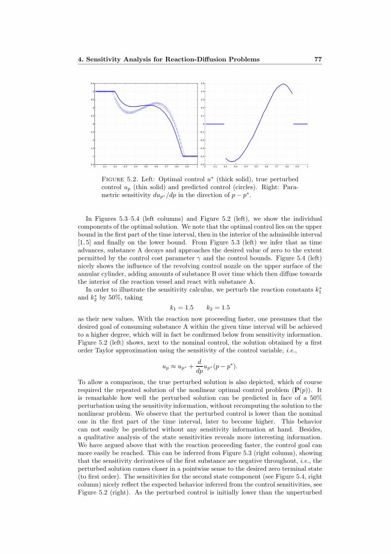
0 0.1 0.2 0.3 0.4 0.5 0.6 0.7 0.8 0.9 10.5

1

1.5

2

2.5

3

3.5

4

4.5

5

5.5

0 0.1 0.2 0.3 0.4 0.5 0.6 0.7 0.8 0.9 1−0.5

−0.4

−0.3

−0.2

−0.1

0

0.1

0.2

0.3

0.4

0.5

Figure 5.2. Left: Optimal control u∗ (thick solid), true perturbedcontrol up (thin solid) and predicted control (circles). Right: Para-metric sensitivity dup∗/dp in the direction of p− p∗.

In Figures 5.3–5.4 (left columns) and Figure 5.2 (left), we show the individualcomponents of the optimal solution. We note that the optimal control lies on the upperbound in the first part of the time interval, then in the interior of the admissible interval[1, 5] and finally on the lower bound. From Figure 5.3 (left) we infer that as timeadvances, substance A decays and approaches the desired value of zero to the extentpermitted by the control cost parameter γ and the control bounds. Figure 5.4 (left)nicely shows the influence of the revolving control nozzle on the upper surface of theannular cylinder, adding amounts of substance B over time which then diffuse towardsthe interior of the reaction vessel and react with substance A.

In order to illustrate the sensitivity calculus, we perturb the reaction constants k∗1and k∗2 by 50%, taking

k1 = 1.5 k2 = 1.5

as their new values. With the reaction now proceeding faster, one presumes that thedesired goal of consuming substance A within the given time interval will be achievedto a higher degree, which will in fact be confirmed below from sensitivity information.Figure 5.2 (left) shows, next to the nominal control, the solution obtained by a firstorder Taylor approximation using the sensitivity of the control variable, i.e.,

up ≈ up∗ +d

dpup∗(p− p∗).

To allow a comparison, the true perturbed solution is also depicted, which of courserequired the repeated solution of the nonlinear optimal control problem (P(p)). Itis remarkable how well the perturbed solution can be predicted in face of a 50%perturbation using the sensitivity information, without recomputing the solution to thenonlinear problem. We observe that the perturbed control is lower than the nominalone in the first part of the time interval, later to become higher. This behaviorcan not easily be predicted without any sensitivity information at hand. Besides,a qualitative analysis of the state sensitivities reveals more interesting information.We have argued above that with the reaction proceeding faster, the control goal canmore easily be reached. This can be inferred from Figure 5.3 (right column), showingthat the sensitivity derivatives of the first substance are negative throughout, i.e., theperturbed solution comes closer in a pointwise sense to the desired zero terminal state(to first order). The sensitivities for the second state component (see Figure 5.4, rightcolumn) nicely reflect the expected behavior inferred from the control sensitivities, seeFigure 5.2 (right). As the perturbed control is initially lower than the unperturbed


Figure 5.3. Concentrations of substance A (left) and its sensitivity(right) at times t = 0.25, t = 0.50, t = 0.75, and t = 1.00.


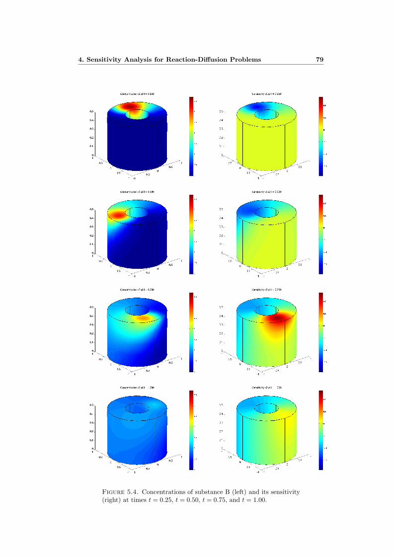
Figure 5.4. Concentrations of substance B (left) and its sensitivity(right) at times t = 0.25, t = 0.50, t = 0.75, and t = 1.00.


one after leaving the upper bound, the sensitivity of the second substance is belowzero there. Later, it becomes positive, as does the sensitivity for the control variable.

References

[1] R. Adams. Sobolev Spaces. Academic Press, New York, 1975.[2] M. Bergounioux, M. Haddou, M. Hintermuller, and K. Kunisch. A comparison of a Moreau-

Yosida-based active set strategy and interior point methods for constrained optimal controlproblems. SIAM Journal on Optimization, 11(2):495–521, 2000.

[3] C. Buskens and R. Griesse. Parametric sensitivity analysis of perturbed PDE optimal controlproblems with state and control constraints. Journal of Optimization Theory and Applications,131(1):17–35, 2006.

[4] E. DiBenedetto. Degenerate Parabolic Equations. Springer, Berlin, 1993.[5] A. Dontchev. Implicit function theorems for generalized equations. Mathematical Programming,

70:91–106, 1995.[6] R. Griesse. Parametric sensitivity analysis in optimal control of a reaction-diffusion system—

Part I: Solution differentiability. Numerical Functional Analysis and Optimization, 25(1–2):93–117, 2004.

[7] R. Griesse. Parametric sensitivity analysis in optimal control of a reaction-diffusion system—Part II: Practical methods and examples. Optimization Methods and Software, 19(2):217–242,2004.

[8] R. Griesse and S. Volkwein. A semi-smooth Newton method for optimal boundary control of anonlinear reaction-diffusion system. In Proceedings of the Sixteenth International Symposium onMathematical Theory of Networks and Systems (MTNS), Leuven, Belgium, 2004.

[9] R. Griesse and S. Volkwein. A primal-dual active set strategy for optimal boundary control of anonlinear reaction-diffusion system. SIAM Journal on Control and Optimization, 44(2):467–494,2005.

[10] M. Hintermuller, K. Ito, and K. Kunisch. The primal-dual active set strategy as a semismoothNewton method. SIAM Journal on Optimization, 13(3):865–888, 2002.

[11] K. Malanowski. Sensitivity analysis for parametric optimal control of semilinear parabolic equa-tions. Journal of Convex Analysis, 9(2):543–561, 2002.

[12] K. Malanowski. Solution differentiability of parametric optimal control for elliptic equations. InE. W. Sachs and R. Tichatschke, editors, System Modeling and Optimization XX, Proceedingsof the 20th IFIP TC 7 Conference, pages 271–285. Kluwer Academic Publishers, 2003.

[13] K. Malanowski and F. Troltzsch. Lipschitz stability of solutions to parametric optimal controlfor parabolic equations. Journal of Analysis and its Applications, 18(2):469–489, 1999.

[14] K. Malanowski and F. Troltzsch. Lipschitz stability of solutions to parametric optimal controlfor elliptic equations. Control and Cybernetics, 29:237–256, 2000.

[15] S. Robinson. Strongly regular generalized equations. Mathematics of Operations Research,5(1):43–62, 1980.

[16] T. Roubıcek and F. Troltzsch. Lipschitz stability of optimal controls for the steady-state Navier-Stokes equations. Control and Cybernetics, 32(3):683–705, 2003.

[17] R. Temam. Navier-Stokes Equations, Theory and Numerical Analysis. North-Holland, Amster-dam, 1984.

[18] F. Troltzsch. Lipschitz stability of solutions of linear-quadratic parabolic control problems withrespect to perturbations. Dynamics of Continuous, Discrete and Impulsive Systems Series AMathematical Analysis, 7(2):289–306, 2000.

[19] M. Ulbrich. Semismooth Newton methods for operator equations in function spaces. SIAM Jour-nal on Control and Optimization, 13(3):805–842, 2003.


CHAPTER 2

Numerical Methods and Applications

Besides their theoretical interest, the concepts of stability and sensitivity of optimiza-tion and of optimal control problems in particular have a number of applications. Weaddress some of them in this chapter, along with numerical methods for the compu-tation of sensitivity derivatives and related quantities.

First of all, Newton’s method, when applied to a generalized equation, exhibits localquadratic convergence whenever the generalized equation

0 ∈ F (w) +N (w)

is strongly regular (see Definition 0.7 on p. 11) and F is sufficiently smooth. In thecontext of optimal control problems, Newton’s method amounts to an SQP (sequentialquadratic programming) approach. Based on our Lipschitz stability results for optimalcontrol problems with mixed control-state constraints (Section 2), we establish thelocal quadratic convergence of SQP for semilinear problems with such constraints inSection 5 below.

In addition, we have considered in Chapter 1 the differentiability of local optimalsolutions of various optimal control problems with control constraints. These problemscan be written in abstract form as

(Pcc(π))

Minimize J(y, u;π)

subject to e(y, u;π) = 0and ua ≤ u ≤ ub a.e.

Using the Implicit Function Theorem 0.6, we have shown in various cases the existenceof a local map

π 7→ Ξ(π) = (Ξy(π),Ξu(π),Ξp(π))

near the nominal parameter π0, which is Lipschitz and directionally differentiable.The computation of one directional derivative DΞ(π0; δπ) amounts to the solution ofa linear-quadratic optimal control problem with the same type of control constraints,compare (DQP(δ, δ)) on p. 9, Theorem 4.1 of Griesse, Hintermuller, and Hinze [2005](Section 3), or Theorem 4.1 of Griesse and Volkwein [2006] (Section 4).

We address in this chapter a number of questions related to these sensitivity deriva-tives:

(1) How can the solution of a perturbed problem Ξ(π) be recovered from thesolution of the nominal problem Ξ(π0) and derivative information, as accu-rately as possible? (Section 6)

(2) What is the worst-case perturbation which has the greatest impact on thesolution or a quantity of interest depending on the solution? (Section 7)

(3) How can first and second-order derivatives of such a quantity of interest beevaluated efficiently? (Section 8)

(4) What is the relationship between the sensitivity derivatives of (Pcc(π)) andof its relaxation arising in interior point approaches? (Section 9)

82 Numerical Methods and Applications

5. Local Quadratic Convergence of SQP for Elliptic Optimal ControlProblems with Mixed Control-State Constraints

R. Griesse, N. Metla and A. Rosch: Local Quadratic Convergence of SQP for El-liptic Optimal Control Problems with Mixed Control-State Constraints, submitted to:ESAIM: Control, Optimisation, and Calculus of Variations, 2007

In this paper, we show the local quadratic convergence behavior of the sequentialquadratic programming (SQP) approach for the solution of semilinear elliptic optimalcontrol problems of the type

(Pmcc)

Minimize∫

Ω

φ(x, y, u) dx

subject toAy + d(x, y) = u in Ω,

y = 0 on Γ.

and

u ≥ 0 in Ω,ε u+ y ≥ yc in Ω,

where A is a uniformly elliptic second-order differential operator and d is a monotonenonlinearity. The SQP method was considered previously for optimal control prob-lems with control constraints only, see for instance Unger [1997], Heinkenschloss andTroltzsch [1998], Troltzsch [1999], Troltzsch and Volkwein [2001], Hintermuller andHinze [2006] and Wachsmuth [2007].

The first-order optimality system for (Pmcc) is a generalization of the system (2.1)for the linear-quadratic problem given on p. 29. It is re-written (see Section 4 of thepaper) as a generalized equation

(5.1) 0 ∈ F (w) +N (w),

where in contrast to the previous cases, F now comprises also the inequality con-straints, and w = (y, u, p, µ1, µ2) comprises state, control and adjoint variables as wellas Lagrange multipliers. This approach would allow nonlinear inequality constraintsas well, which will be considered in an upcoming publication.

Given a current iterate wk, Newton’s method, applied to (5.1), produces the newiterate as a solution of

(5.2) 0 ∈ F (wk) + F ′(wk)(wk+1 − wk) +N (wk+1).

It can be verified that (5.2) is equivalent to one step of the SQP method (see Section 5of the paper). However, for the convergence analysis it is convenient to think in termsof Newton’s method. Let us briefly outline how the local quadratic convergence isshown, compare Alt [1990, 1994]. Suppose that w∗ is a solution of (5.1). We write theNewton step (5.2) as a perturbed step taken at w∗:

(5.3) δk+1 ∈ F (w∗) + F ′(w∗)(wk+1 − w∗) +N(wk+1)

where

δk+1 := F (w∗)− F (wk) + F ′(w∗)(wk+1 − w∗)− F ′(wk)(wk+1 − wk).

By the fact that w∗ is a solution of (5.1), it also solves

(5.4) 0 ∈ F (w∗) + F ′(w∗)(w∗ − w∗) +N(w∗),

Under the condition that (5.1) is strongly regular at w∗, we get from (5.3) and (5.4)that

(5.5) ‖wk+1 − w∗‖ ≤ L ‖δk+1‖It remains to show that

‖δk+1‖ ≤ c1 ‖wk+1 − wk‖2 + c2 ‖wk − w∗‖‖wk+1 − w∗‖,

5. SQP for Mixed-Constrained Optimal Control Problems 83

which follows from differentiability and Lipschitz properties of F , i.e., from the prop-erties of d and φ. Given that ‖wk − w∗‖ is sufficiently small, the second term can behidden in the left hand side of (5.5), which yields the local quadratic convergence.

The strong regularity of (5.1) at w∗ follows from our results in Alt et al. [2006], seeSection 2 of this thesis, under the assumption that the active sets at the solution w∗

are well separated and that second-order sufficient conditions hold, see Theorem 6.7of the paper under discussion.

LOCAL QUADRATIC CONVERGENCE OF SQP FOR ELLIPTICOPTIMAL CONTROL PROBLEMS WITH MIXED

CONTROL-STATE CONSTRAINTS

ROLAND GRIESSE, NATALIYA METLA, AND ARND ROSCH

Abstract. Semilinear elliptic optimal control problems with pointwise control

and mixed control-state constraints are considered. Necessary and sufficient op-

timality conditions are given. The equivalence of the SQP method and Newton’s

method for a generalized equation is discussed. Local quadratic convergence of

the SQP method is proved.

1. Introduction

This paper is concerned with the local convergence analysis of the sequential qua-dratic programming (SQP) method for the following class of semilinear optimal controlproblems:

Minimize f(y, u) :=∫

Ω

φ(ξ, y(ξ), u(ξ)) dξ (P)

subject to u ∈ L∞(Ω) and the elliptic state equation

A y + d(ξ, y) = u in Ω,

y = 0 on ∂Ω,(1.1)

as well as pointwise constraints

u > 0 in Ω,

εu + y > yc in Ω.(1.2)

Here and throughout, Ω is a bounded domain in RN , N ∈ 2, 3, which is convex orhas a C1,1 boundary ∂Ω. In (1.1), A is an elliptic operator in H1

0 (Ω) specified below,and ε is a positive number. The bound yc is a function in L∞(Ω).

Problems with mixed control-state constraints are important as Lavrientiev-typeregularizations of pointwise state-constrained problems [10–12], but they are also in-teresting in their own right. In the former case, ε is a small parameter tending tozero. For the purpose of this paper, we consider ε to be fixed. Note that in additionto the mixed control-state constraint, a pure control constraint is present on the samedomain. Since problem (P) is nonconvex, different local minima may occur.

SQP methods have proved to be fast solution methods for nonlinear programmingproblems. A large body of literature exists concerning the analysis of these methodsfor finite-dimensional problems. For a convergence analysis in a general Banach spacesetting with equality and inequality constraints, we refer to [2, 3].

The main contribution of this paper is the proof of local quadratic convergence ofthe SQP method, applied to (P). To our knowledge, such convergence results in thecontext of PDE-constrained optimization are so far only available for purely control-constrained problems [7, 17, 19]. Following [2], we exploit the equivalence betweenthe SQP and the Lagrange-Newton methods, i.e., Newton’s method, applied to ageneralized (set-valued) equation representing necessary conditions of optimality. Weconcentrate on specific issues arising due to the semilinear state equation, e.g., the


careful choice of suitable function spaces. An important step is the verification of theso-called strong regularity of the generalized equation, which is made difficult by thesimultaneous presence of pure control and mixed control-state constraints (1.2). Thekey idea was recently developed in [4].

We remark that strong regularity is known to be closely related to second-ordersufficient conditions (SSC). For problems with pure control constraints, SSC are wellunderstood and they are close to the necessary ones when so-called strongly activesubsets are used, see, e.g., [17, 19, 20]. However, the situation is more difficult forproblems with mixed control-state constraints [14, 16] or even pure state constraints.In order to avoid a more technical discussion, we presently employ relatively strongSSC and refer to future work for their refinement. We also refer to an upcomingpublication concerning the numerical application of the SQP method to problems oftype (P).

The material in this paper is organized as follows. In Section 2, we state ourmain assumptions and recall some properties about the state equation. Necessaryand sufficient optimality conditions for problem (P) are stated in Section 3, and theirreformulation as a generalized equation is given in Section 4. Section 5 addresses theequivalence of the SQP and Lagrange-Newton methods. Section 6 is devoted to theproof of strong regularity of the generalized equation. Finally, Section 7 completes theconvergence analysis of the SQP method. A number of auxiliary results have beencollected in the Appendix.

We denote by Lp(Ω) and Hm(Ω) the usual Lebesgue and Sobolev spaces [1], and(·, ·) is the scalar product in L2(Ω) or [L2(Ω)]N , respectively. H1

0 (Ω) is the subspace ofH1(Ω) with zero boundary traces, and H−1(Ω) is its dual. The continuous embeddingof a normed space X into a normed space Y is denoted by X → Y . Throughout, wedenote by BX

r (x) the open ball of radius r around x, in the topology of X. In particular,we write B∞

r (x) for the open ball with respect to the L∞(Ω) norm. Throughout, c,c1 etc. denote generic positive constants whose value may change from instance toinstance.

2. Assumptions and Properties of the State Equation

The following assumptions (A1)–(A4) are taken to hold throughout the paper.

Assumption.(A1) Let Ω be a bounded domain in RN , N ∈ 2, 3 which is convex or has C1,1

boundary ∂Ω. The bound yc is in L∞(Ω), and ε > 0.

(A2) The operator A : H10 (Ω) → H−1(Ω) is defined as A y(v) = a[y, v], where

a[y, v] = ((∇v), A0∇y) + (b>∇y, v) + (cy, v).

A0 is an N × N matrix with Lipschitz continuous entries on Ω such thatρ>A0(ξ) ρ > m0 |ρ|2 holds with some m0 > 0 for all ρ ∈ RN and almost allξ ∈ Ω. Moreover, b ∈ L∞(Ω)N and c ∈ L∞(Ω). The bilinear form a[·, ·] is notnecessarily symmetric but it is assumed to be continuous and coercive, i.e.,

a[y, v] 6 c ‖y‖H1(Ω) ‖v‖H1(Ω)

a[y, y] > c ‖y‖2H1(Ω)

for all y, v ∈ H10 (Ω) with some positive constants c and c. A simple example

is a[y, v] = (∇y,∇v), corresponding to A = −∆.

(A3) d(ξ, y) belongs to the C2-class of functions with respect to y for almost allξ ∈ Ω. Moreover, dyy is assumed be a locally bounded and locally Lipschitz-continuous function with respect to y, i.e., the following conditions hold true:


there exists K > 0 such that

|d(ξ, 0)|+ |dy(ξ, 0)|+ |dyy(ξ, 0)| 6 Kd,

and for any M > 0, there exists Ld(M) > 0 such that

|dyy(ξ, y1)− dyy(ξ, y2)| 6 Ld(M) |y1 − y2| a.e. in Ω

for all y1, y2 ∈ R satisfying |y1|, |y2| 6 M .

Additionally dy(ξ, y) > 0 a.e. in Ω, for all y ∈ R.

(A4) The function φ = φ(ξ, y, u) is measurable with respect to ξ ∈ Ω for eachy and u, and of class C2 with respect to y and u for almost all ξ ∈ Ω.Moreover, the second derivatives are assumed to be locally bounded and lo-cally Lipschitz-continuous functions, i.e., the following conditions hold: thereexist Ky,Ku,Kyu > 0 such that

|φ(ξ, 0, 0)|+ |φy(ξ, 0, 0)|+ |φyy(ξ, 0, 0)| 6 Ky, |φyu(ξ, 0, 0)| 6 Kyu,

|φ(ξ, 0, 0)|+ |φu(ξ, 0, 0)|+ |φuu(ξ, 0, 0)| 6 Ku,

Moreover, for any M > 0, there exists Lφ(M) > 0 such that

|φyy(ξ, y1, u1)− φyy(ξ, y2, u2)| 6 Lφ(M)(|y1 − y2|+ |u1 − u2|

),

|φyu(ξ, y1, u1)− φyu(ξ, y2, u2)| 6 Lφ(M)(|y1 − y2|+ |u1 − u2|

),

|φuy(ξ, y1, u1)− φuy(ξ, y2, u2)| 6 Lφ(M)(|y1 − y2|+ |u1 − u2|

),

|φuu(ξ, y1, u1)− φuu(ξ, y2, u2)| 6 Lφ(M)(|y1 − y2|+ |u1 − u2|

)for all yi, ui ∈ R satisfying |yi|, |ui| 6 M , i = 1, 2.

In addition, φuu(ξ, y, u) > m > 0 a.e. in Ω, for all (y, u) ∈ R2.

In the sequel, we will simply write d(y) instead of d(ξ, y) etc. As a consequence of(A3)–(A4), the Nemyckii operators d(·) and φ(·) are twice continuously Frechet differ-entiable with respect to the L∞(Ω) norms, and their derivatives are locally Lipschitzcontinuous, see Lemma A.1.

The necessity of using L∞(Ω) norms for general nonlinearities d and φ motivatesour choice

Y := H2(Ω) ∩H10 (Ω)

as a state space, since Y → L∞(Ω).

Remark 2.1. In case Ω has only a Lipschitz boundary, our results remain true whenY is replaced by H1

0 (Ω) ∩ L∞(Ω).

Recall that a function y ∈ H10 (Ω)∩L∞(Ω) is called a weak solution of (1.1) with

u ∈ L2(Ω) if a[y, v] + (d(y), v) = (u, v) holds for all v ∈ H10 (Ω).

Lemma 2.2. Under assumptions (A1)–(A3) and for any given u ∈ L2(Ω), the semi-linear equation (1.1) possesses a unique weak solution y ∈ Y . It satisfies the a prioriestimate

‖y‖H1(Ω) + ‖y‖L∞(Ω) 6 CΩ

(‖u‖L2(Ω) + 1)

with a constant CΩ independent of u.

Proof. The existence and uniqueness of a weak solution y ∈ H10 (Ω) ∩ L∞(Ω) is a

standard result [18, Theorem 4.8]. It satisfies

‖y‖H1(Ω) + ‖y‖L∞(Ω) 6 CΩ (‖u‖L2(Ω) + 1) =: M

with some constant CΩ independent of u. Lemma A.1 implies that d(y) ∈ L∞(Ω).Using the embedding L∞(Ω) → L2(Ω), we conclude that the difference u−d(y) belongsto L2(Ω). Owing to assumption (A1), y ∈ H2(Ω), see for instance [6, Theorem 2.2.2.3].


We will frequently also need the corresponding result for the linearized equation

A y + dy(y) y = u in Ω,

y = 0 on ∂Ω.(2.1)

Lemma 2.3. Under assumptions (A1)–(A3) and given y ∈ L∞(Ω), the linearizedPDE (2.1) possesses a unique weak solution y ∈ Y for any given u ∈ L2(Ω). Itsatisfies the a priori estimate

‖y‖H2(Ω) 6 CΩ(y) ‖u‖L2(Ω)

with a constant CΩ(y) independent of u.

Proof. According to (A3) and Lemma A.1, dy(y) is a nonnegative coefficient in L∞(Ω).The claim thus follows again from standard arguments, see, e.g., [6, Theorem 2.2.2.3].

3. Necessary and Sufficient Optimality Conditions

In this section, we introduce necessary and sufficient optimality conditions for prob-lem (P). For convenience, we define the Lagrange functional

L : Y × L∞(Ω)× Y × L∞(Ω)× L∞(Ω) → R

as

L(y, u, p, µ1, µ2) = f(y, u) + a[y, p] + (p, d(y)− u)− (µ1, u)− (µ2, εu + y − yc).

Here, µi are Lagrange multipliers associated to the inequality constraints, and p isthe adjoint state. The existence of regular Lagrange multipliers µ1, µ2 ∈ L∞(Ω) wasshown in [15, Theorem 7.3], which implies the following lemma:

Lemma 3.1. Suppose that (y, u) ∈ Y × L∞(Ω) is a local optimal solution of (P).Then there exist regular Lagrange multipliers µ1, µ2 ∈ L∞(Ω) and an adjoint statep ∈ Y such that the first-oder necessary optimality conditions

Ly(y, u, p, µ1, µ2) = 0, Lu(y, u, p, µ1, µ2) = 0, Lp(y, u, p, µ1, µ2) = 0,

u > 0, µ1 > 0, µ1u = 0,

εu + y − yc > 0, µ2 > 0, µ2(εu + y − yc) = 0

(FON)

hold.

Remark 3.2. The Lagrange multipliers and adjoint state associated to a local optimalsolution of (P) need not be unique if the active sets ξ ∈ Ω : u = 0 and ξ ∈ Ω : εu+y− yc = 0 intersect nontrivially. This situation will be excluded by Assumption (A6)below.

Conditions (FON) are also stated in explicit form in (4.1) below. To guaranteethat x = (y, u) with associated multipliers λ = (µ1, µ2, p) is a local solution of (P),we introduce the following second-order sufficient optimality condition (SSC):

There exists a constant α > 0 such that

Lxx(x, λ)(δx, δx) > α ‖δx‖2[L2(Ω)]2 (3.1)

for all δx = (δy, δu) ∈ Y × L∞(Ω) which satisfy the linearized equation

Aδy + dy(y) · δy = δu in Ω,

δy = 0 on ∂Ω.(3.2)

In (3.1), the Hessian of the Lagrange functional is given by

Lxx(x, λ)(δx, δx) :=∫

Ω

(δy

δu

)>(φyy(y, u) + dyy(y) p φyu(y, u)

φuy(y, u) φuu(y, u)

)(δy

δu

)dξ.


For convenience, we will use the abbreviation

X := Y × L∞(Ω) = H2(Ω) ∩H10 (Ω)× L∞(Ω)

in the sequel.

Assumption.

(A5) We assume that x∗ = (y∗, u∗) ∈ X, together with associated Lagrange multi-pliers λ∗ = (p∗, µ∗1, µ

∗2) ∈ Y × [L∞(Ω)]2, satisfies both (FON) and (SSC).

As mentioned in the introduction, we are aware of the fact that there exist weakersufficient conditions which take into account strongly active sets. However, this furthercomplicates the convergence analysis of SQP and is therefore postponed to later work.

Definition 3.3.

(a) A pair x = (y, u) ∈ X is called an admissible point if it satisfies (1.1) and(1.2).

(b) A point x ∈ X is called a strict local optimal solution in the sense ofL∞(Ω) if there exists ε > 0 such that the inequality f(x) < f(x) holds for alladmissible x ∈ X \ x with ‖x− x‖[L∞(Ω)]2 6 ε.

Theorem 3.4. Under Assumptions (A1)–(A5), there exists β > 0 and ε > 0 suchthat

f(x) > f(x∗) + β ‖x− x∗‖2[L2(Ω)]2

holds for all admissible x ∈ X with ‖x− x∗‖[L∞(Ω)]2 6 ε. In particular, x∗ is a strictlocal optimal solution in the sense of L∞(Ω).

Proof. The proof uses the two-norm discrepancy principle, see [8, Theorem 3.5]. Letx ∈ X be an admissible point, which implies

a[y, p∗] + (p∗, d(y)− u) = 0and u > 0, εu + y − yc > 0 a.e. in Ω.

In view of µ∗1, µ∗2 > 0, we can estimate the cost functional f by the Lagrange functional:

f(x) > f(x) + a[y, p∗] + (p∗, d(y)− u)− (µ∗1, u)− (µ∗2, εu + y − yc) = L(x, λ∗). (3.3)

The Lagrange functional is twice continuously differentiable with respect to the L∞(Ω)norms, as is easily seen from Lemma A.1. Hence it possesses a Taylor expansion

L(x, λ∗) = L(x∗, λ∗) + Lx(x∗, λ∗)(x− x∗) + Lxx(x + θ(x− x∗), λ∗)(x− x∗, x− x∗)

for all x ∈ X, where θ ∈ (0, 1). Since the pair (x∗, λ∗) satisfies (FON), we have

f(x∗) = L(x∗, λ∗) + Lx(x∗, λ)(x− x∗),

which implies

L(x, λ∗) = f(x∗) + Lxx(x∗, λ∗)(x− x∗, x− x∗)

+(Lxx(x∗ + θ(x− x∗), λ∗)− Lxx(x∗, λ∗)

)(x− x∗, x− x∗).

We cannot use (SSC) directly since x satisfies the semilinear equation (1.1) insteadof the linearized one (3.2). However, Lemma A.2 implies that there exist ε > 0 andα′ > 0 such that

L(x, λ∗) > f(x∗) + α′ ‖x− x∗‖2[L2(Ω)]2

+(Lxx(x∗ + θ(x− x∗), λ∗)− Lxx(x∗, λ∗)

)(x− x∗, x− x∗), (3.4)


given that ‖x− x∗‖[L∞(Ω)]2 6 ε. Moreover, the Hessian of the Lagrange functional sat-isfies the following local Lipschitz condition (see Lemma A.1 and also [18, Lemma 4.24]):

|(Lxx(x∗ + θ(x− x∗), λ∗)− Lxx(x∗, λ∗))(x− x∗, x− x∗)|6 c ‖x− x∗‖[L∞(Ω)]2 ‖x− x∗‖2

[L2(Ω)]2 (3.5)

for all ‖x− x∗‖[L∞(Ω)]2 6 ε. Summarizing (3.3)–(3.5), we can estimate

f(x) > f(x∗) + β ‖x− x∗‖2[L2(Ω)]2 ,

where

β := α′ − c ‖x− x∗‖[L∞(Ω)]2 > α′ − c ε > 0

when ε is taken sufficiently small.

4. Generalized Equation

We recall the necessary optimality conditions (FON) for problem (P), which readin explicit form

a[v, p] + (dy(y)p, v) + (φy(y, u), v)− (µ2, v) = 0, v ∈ H10 (Ω)

(φu(y, u), v)− (p, v)− (µ1, v)− (εµ2, v) = 0, v ∈ L2(Ω)

a[y, v] + (d(y), v)− (u, v) = 0, v ∈ H10 (Ω)

µ1 > 0, u > 0, µ1u = 0

µ2 > 0, εu + y − yc > 0, µ2(εu + y − yc) = 0

a.e. in Ω.

(4.1)

As was mentioned in the introduction, the local convergence analysis of SQP is basedon its interpretation as Newton’s method for a generalized (set-valued) equation

0 ∈ F (y, u, p, µ1, µ2) + N(y, u, p, µ1, µ2) (4.2)

equivalent to (4.1). We define

K := µ ∈ L∞(Ω) : µ > 0 a.e. in Ω,the cone of nonnegative functions in L∞(Ω), and the dual cone N1 : L∞(Ω) −→P (L∞(Ω)),

N1(µ) :=

z ∈ L∞(Ω) : (z, µ− ν) > 0 ∀ν ∈ K if µ ∈ K,

∅ if µ 6∈ K.

Here P (L∞) denotes the power set of L∞(Ω), i.e., the set of all subsets of L∞(Ω).In (4.2), F contains the single-valued part of (4.1), i.e.,

F (y, u, p, µ1, µ2)(·) =

a[·, p] + (dy(y) p, ·) + (φy(y, u), ·)− (µ2, ·)

φu(y, u)− p− µ1 − εµ2

a[y, ·] + (d(y), ·)− (u, ·)u

εu + y − yc

and N is a set-valued function

N(y, u, p, µ1, µ2) = (0, 0, 0, N1(µ1), N1(µ2))>.

Note that the generalized equation (4.2) is nonlinear, since it contains the nonlinearfunctions d, dy, φy and φu.


Remark 4.1. Let

W := Y × L∞(Ω)× Y × L∞(Ω)× L∞(Ω),

Z := L2(Ω)× L∞(Ω)× L2(Ω)× L∞(Ω)× L∞(Ω).

Then F : W −→ Z and N : W −→ P (Z). Owing to Assumptions (A3) and (A4), F iscontinuously Frechet differentiable with respect to the L∞(Ω) norms, see Lemma A.1.

Lemma 4.2. The first-order necessary conditions (4.1) and the generalized equation(4.2) are equivalent.

Proof. (4.2) ⇒ (4.1): This is immediate for the first three components. For the fourthcomponent we have

− u ∈ N1(µ1)

⇒ µ1 ∈ K and (−u, µ1 − ν) > 0 for all ν ∈ K

⇒ µ1(ξ) > 0 and − u(ξ)(µ1(ξ)− ν) > 0 for all ν > 0, a.e. in Ω.

This impliesµ1(ξ) = 0 ⇒ u(ξ) > 0

µ1(ξ) > 0 ⇒ u(ξ) = 0,

which shows the first complementarity system in (4.1). The second follows analogously.(4.1) ⇒ (4.2): This is again immediate for the first three components. From the

first complementarity system in (4.1) we infer that

u(ξ) ν > 0 for all ν > 0, a.e. in Ω

⇒ − u(ξ)(µ1(ξ)− ν) > 0 for all ν > 0, a.e. in Ω

⇒ − (u, µ1 − ν) > 0 for all ν ∈ K.

In view of µ1 ∈ K, this implies −u ∈ N1(µ1). Again, −(εu + y − yc) ∈ N1(µ2) followsanalogously.

5. SQP Method

In this section we briefly recall the SQP (sequential quadratic programming) methodfor the solution of problem (P). We also discuss its equivalence with Newton’s method,applied to the generalized equation (4.2), which is often called the Lagrange-Newtonapproach. Throughout the rest of the paper we use the notation

wk := (xk, λk) = (yk, uk, pk, µk1 , µk

2) ∈ W

to denote an iterate of either method. SQP methods break down the solution of (P)into a sequence of quadratic programming problems. At any given iterate wk, onesolves

Minimize fx(xk)(x− xk) +12Lxx(xk, λk)(x− xk, x− xk) (QPk)

subject to x = (y, u) ∈ Y × L∞(Ω), the linear state equation

A y + d(yk) + dy(yk)(y − yk) = u in Ω,

y = 0 on ∂Ω,(5.1)

and inequality constraints

u > 0 in Ω,

εu + y − yc > 0 in Ω.(5.2)

The solution (which needs to be shown to exist)

x = (y, u) ∈ Y × L∞(Ω),


together with the adjoint state and Lagrange multipliers

λ = (p, µ1, µ2) ∈ Y × L∞(Ω)× L∞(Ω),

will serve as the next iterate wk+1.

Lemma 5.1. There exists R > 0 such that (QPk) has a unique global solution x =(y, u) ∈ X, provided that (xk, pk) ∈ B∞

R (x∗, p∗).

Proof. For every u ∈ L2(Ω), the linearized PDE (5.1) has a unique solution y ∈ Y byLemma 2.3. We define the feasible set

Mk := x = (y, u) ∈ Y × L2(Ω) satisfying (5.1) and (5.2).The set Mk is non-empty, which follows from [4, Lemma 2.3] using δ3 = −d(yk) +dy(yk) yk. The proof uses the maximum principle for the differential operator Ay +dy(yk) y. Clearly, Mk is also closed and convex.

The cost functional of (QPk) can be decomposed into quadratic and affine parts inx. Lemma A.3 shows that there exists R > 0 and α′′ > 0 such that

Lxx(xk, λk)(x, x

)> α′′ ‖x‖2

[L2(Ω)]2

for all (y, u) ∈ X satisfying A y + dy(yk) y = u in Ω with homogeneous Dirichletboundary conditions, provided that (xk, pk) ∈ B∞

R (x∗, p∗). This implies that thecost functional is uniformly convex, continuous (i.e., weakly lower semicontinuous)and radially unbounded, which shows the unique solvability of (QPk) in Y × L2(Ω).Using the optimality system (5.3) below, we can conclude as in [4, Lemma 2.7] thatu ∈ L∞(Ω).

The solution (y, u) of (QPk) and its Lagrange multipliers (p, µ1, µ2) are character-ized by the first order optimality system (compare [4, Lemma 2.5]):

a[v, p] + (dy(yk) p, v) + (φy(yk, uk), v) + (φyu(yk, uk)(u− uk), v)

+((φyy(yk, uk) + dyy(yk) pk)(y − yk), v

)− (µ2, v) = 0, v ∈ H10 (Ω)

(φu(yk, uk), v) + (φuu(yk, uk)(u− uk), v)

+(φuy(yk, uk)(y − yk), v)− (p, v)− (µ1, v)− (εµ2, v) = 0, v ∈ L2(Ω)

a[y, v] + (d(yk), v) + (dy(yk)(y − yk), v)− (u, v) = 0, v ∈ H10 (Ω)

µ1 > 0, u > 0, µ1u = 0

µ2 > 0, εu + y − yc > 0, µ2(εu + y − yc) = 0

a.e. in Ω.

(5.3)

Note that due to the convexity of the cost functional, (5.3) is both necessary andsufficient for optimality, provided that (xk, pk) ∈ B∞

R (x∗, p∗).

Remark 5.2. The Lagrange multipliers (µ1, µ2) and the adjoint state p in (5.3) neednot be unique, compare [4, Remark 2.6]. Non-uniqueness can occur only if µ1 and µ2

are simulateneously nonzero on a set of positive measure.

We recall for convenience the generalized equation (4.2),

0 ∈ F (w) + N(w). (5.4)

Given the iterate wk, Newton’s method yields the next iterate wk+1 as the solution ofthe linearized generalized equation

0 ∈ F (wk) + F ′(wk)(w − wk) + N(w). (5.5)

Analogously to Lemma 4.2, one can show:

Lemma 5.3. System (5.3) and the linearized generalized equation (5.5) are equivalent.


6. Strong Regularity

The local convergence analysis of Newton’s method (5.5) for the solution of (5.4)is based on a perturbation argument. It will be carried out in Section 7. The mainingredient in the proof is the local Lipschitz stability of solutions w = w(η) of

0 ∈ F (η) + F ′(η)(w − η) + N(w) (6.1)

with respect to the parameter η near w∗. The difficulty arises due to the fact that ηenters nonlinearly in (6.1). Therefore, we employ an implicit function theorem due toDontchev [5] to derive this result. This theorem requires the so-called strong regularityof (5.4), i.e., the Lipschitz stability of solutions w = w(δ) of

δ ∈ F (w∗) + F ′(w∗)(w − w∗) + N(w) (6.2)

with respect to the new perturbation parameter δ, which enters linearly. The param-eter δ belongs to the image space of F

Z := L2(Ω)× L∞(Ω)× L2(Ω)× L∞(Ω)× L∞(Ω),

see Remark 4.1. Note that w∗ is a solution of both (5.4) and (6.2) for δ = 0.

Definition 6.1 (see [13]). The generalized equation (5.4) is called strongly regularat w∗ if there exist radii r1 > 0, r2 > 0 and a positive constant Lδ such that for allperturbations δ ∈ BZ

r1(0), the following hold:

(1) the linearized equation (6.2) has a solution wδ = w(δ) ∈ BWr2

(w∗)(2) wδ is the only solution of (6.2) in BW

r2(w∗)

(3) wδ satisfies the Lipschitz condition

‖wδ − wδ′‖W 6 Lδ ‖δ − δ′‖Z for all δ, δ′ ∈ BZr1

(0).

The verification of strong regularity is based on the interpretation of (6.2) as theoptimality system of the following QP problem, which depends on the perturbation δ:

Minimize fx(x∗)(x− x∗) +12Lxx(x∗, λ∗)

(x− x∗, x− x∗

)(LQP(δ))

− ([δ1, δ2], x− x∗)

subject to x = (y, u) ∈ Y × L∞(Ω), the linear state equation

A y + d(y∗) + dy(y∗)(y − y∗) = u + δ3 in Ω,

y = 0 on ∂Ω,(6.3)

and inequality constraints

u > δ4 in Ω,

εu + y − yc > δ5 in Ω.(6.4)

As before, it is easy to check that the necessary optimality conditions of (LQP(δ))are equivalent to (6.2).

Lemma 6.2. For any δ ∈ Z, problem (LQP(δ)) possesses a unique global solutionxδ = (yδ, uδ) ∈ X. If λδ = (pδ, µ1,δ, µ2,δ) ∈ Y × L∞(Ω) × L∞(Ω) are associatedLagrange multipliers, then (xδ, λδ) satisfies (6.2). On other hand, if any (xδ, λδ) ∈ Wsatisfies (6.2), then xδ is the unique global solution of (LQP(δ)), and λδ are associatedadjoint state and Lagrange multipliers.

Proof. For any given δ ∈ Z, let us denote by Mδ the set of all x = (y, u) ∈ Y ×L2(Ω)satisfying (6.3) and (6.4). Then Mδ is nonempty (as can be shown along the lines


of [4, Lemma 2.3]), convex and closed. Moreover, (A5) implies that the cost functionalfδ(x) of (LQP(δ)) satisfies

fδ(x) > α

2‖x‖2

[L2(Ω)]2 + linear terms in x

for all x satisfying (6.3). As in the proof of Lemma 5.1, we conclude that (LQP(δ))has a unique solution xδ = (yδ, uδ) ∈ X.

Suppose that λδ = (pδ, µ1,δ, µ2,δ) ∈ Y × L∞(Ω) × L∞(Ω) are associated Lagrangemultipliers, i.e., the necessary optimality conditions of (LQP(δ)) are satisfied. Asargued above, it is easy to check that then (6.2) holds. On the other hand, suppose thatany (xδ, λδ) ∈ W satisfies (6.2), i.e., the necessary optimality conditions of (LQP(δ)).As fδ is strictly convex, these conditions are likewise sufficient for optimality, and theminimizer xδ is unique.

The proof of Lipschitz stability of solutions for problems of type (LQP(δ)) hasrecently been achieved in [4]. The main difficulty consisted in overcoming the non-uniqueness of the associated adjoint state and Lagrange multipliers. We follow thesame technique here.

Definition 6.3. Let σ > 0 be real number. We define two subsets of Ω,

Sσ1 = ξ ∈ Ω : 0 6 u∗(ξ) 6 σ

Sσ2 = ξ ∈ Ω : 0 6 εu∗(ξ) + y∗(ξ)− yc(ξ) 6 σ,

called the security sets of level σ for (P).

Assumption.

(A6) We require that Sσ1 ∩ Sσ

2 = ∅ for some fixed σ > 0.

From now on, we suppose (A1)–(A6) to hold. Assumption (A6) implies that theactive sets

A∗1 = ξ ∈ Ω : u∗(ξ) = 0A∗2 = ξ ∈ Ω : εu∗(ξ) + y∗(ξ)− yc(ξ) = 0

are well separated. This in turn implies the uniqueness of the Lagrange multipliersand adjoint state (p∗, µ∗1, µ

∗2). Due to a continuity argument, the same conclusions

hold for the solution and Lagrange multipliers of (LQP(δ)) for sufficiently small δ, asproved in the following theorem.

Theorem 6.4. There exist G > 0 and Lδ > 0 such that ‖δ‖Z 6 G σ implies:(1) The Lagrange multipliers λδ = (pδ, µ1,δ, µ2,δ) for (LQP(δ)) are unique.(2) For any such δ and δ′, the corresponding solutions and Lagrange multipliers

of (LQP(δ)) satisfy

‖xδ′ − xδ‖Y×L∞(Ω) + ‖λδ′ − λδ‖Y×L∞(Ω)×L∞(Ω) 6 Lδ ‖δ′ − δ‖Z . (6.5)

Proof. The proof employs the technique introduced in [4], so we will only revisit themain steps here. In contrast to the linear quadratic problem considered in [4], the costfunctional and PDE in (LQP(δ)) are slightly more general. To overcome potentialnon-uniqueness of Lagrange multipliers, one introduces an auxiliary problem withsolutions (yaux

δ , uauxδ ), in which the inequality constraints (6.4) are considered only on

the disjoint sets Sσ1 and Sσ

2 , respectively. Then the associated Lagrange multipliersµaux

i,δ , i = 1, 2, and adjoint state pauxδ are unique, see [4, Lemma 3.1]. For any two

perturbations δ, δ′ ∈ Z we abbreviate

δu := uauxδ − uaux

δ′


and similarly for the remaining quantitites. From the optimality conditions of theauxiliary problem one deduces

α (‖δy‖2L2(Ω) + ‖δu‖2

L2(Ω))(A5)

6 Lxx(y∗, u∗)(δx, δx)

= (δ′1 − δ1, δy) + (δ′2 − δ2, δu)− (δ′3 − δ3, δp)

+ (δµ2, δy) + (δµ1, δu) + ε (δµ2, δu)

6 (δ′1 − δ1, δy) + (δ′2 − δ2, δu)− (δ′3 − δ3, δp)

+ (δµ1, δ′4 − δ4) + (δµ2, δ

′5 − δ5).

The last inequality follows from [4, Lemma 3.3]. Young’s inequality yields

α

2(‖δy‖2

L2(Ω) + ‖δu‖2L2(Ω))

6 max 2

α,

14κ

‖δ − δ′‖2[L2(Ω)]5 + κ

( ‖δp‖2L2(Ω) + ‖δµ1‖2

L2(Ω) + ‖δµ2‖2L2(Ω)

), (6.6)

where κ > 0 is specified below. The difference of the adjoint states satisfies

a[v, δp] + (dy(y∗) δp, v) = −(φyy(y∗, u∗) δy, v)− (dyy(y∗) p∗ δy, v)

− (φyu(y∗, u∗) δu, v) + (δ1 − δ′1, v) + (δµ2, v) (6.7)

for all v ∈ H10 (Ω). The differences in the Lagrange multipliers are given by

δµ1 =

φuu(y∗, u∗) δu + φuy(y∗, u∗) δy − δp− (δ2 − δ′2) in Sσ1

0 in Ω \ Sσ1

(6.8)

and

εδµ2 =

φuu(y∗, u∗) δu + φuy(y∗, u∗) δy − δp− (δ2 − δ′2) in Sσ2 ,

0 in Ω \ Sσ2

(6.9)

The substitution of δµ2 into (6.7) yields

a[v, δp] + (dy(y∗) δp, v) +1ε(δp, χSσ

2· v)

= −(φyy(y∗, u∗) δy, v)− (dyy(y∗) p∗, δy)− φyu(y∗, u∗) δu + (δ1 − δ′1, v)

+1ε(φuu(y∗, u∗) δu, χSσ

2· v) +

1ε(φuy(y∗, u∗) δy, χSσ

2· v)− (δ2 − δ′2, χSσ

2· v).

A standard a priori estimate (compare Lemma 2.3) implies

‖δp‖L2(Ω) 6 ‖δp‖Y 6 c( ‖δy‖L2(Ω) + ‖δu‖L2(Ω) + ‖δ1 − δ′1‖L2(Ω) + ‖δ2 − δ′2‖L2(Ω)

).

From (6.8) and (6.9), we infer that ‖δµ1‖L2(Ω) and ‖δµ2‖L2(Ω) can be estimated asimilar expression. Plugging these estimates into (6.6), and choosing κ sufficientlysmall, we get

‖δy‖2L2(Ω) + ‖δu‖2

L2(Ω) 6 caux ‖δ − δ′‖2[L2(Ω)]5 .

By a priori estimates for the linearized and adjoint PDEs, we immediately obtainLipschitz stability for δy and thus for δp with respect to the H2(Ω)-norm.

The projection formula (compare [4, Lemma 2.7] and also Lemma A.1)

µaux1,δ + εµaux

2,δ = max

0, φuu(y∗, u∗)(max

δ4,

yc + δ5 − yauxδ

ε

− u∗)

+ φuy(y∗, u∗) (yauxδ − y∗) + φu(y∗, u∗)− paux

δ − δ2

yields the L∞(Ω)-regularity for the Lagrange multipliers (µaux

1,δ , µaux2,δ ) and the control

uauxδ . As in [4, Lemma 3.5], we conclude

‖δµ1 + ε δµ2‖L∞(Ω) 6 c ‖δ′ − δ‖Z .


From the optimality system we have

φuu(y∗, u∗) δu = δµ1 + ε δµ2 − φuy(y∗, u∗) δy + δp + (δ2 − δ′2),

which implies by Assumption (A4)

m ‖δu‖L∞(Ω) 6 c( ‖δµ1 + ε δµ2‖L∞(Ω) + ‖δy‖L∞(Ω) + ‖δp‖L∞(Ω) + ‖δ2 − δ′2‖L∞(Ω)

)and yields the desired L∞-stability for the control of the auxiliary problem.

As in [4, Lemma 4.1], one shows that for ‖δ‖Z 6 G σ (for a certain constantG > 0), the solution (yaux

δ , uauxδ ) of the auxiliary problem coincides with the solution

of (LQP(δ)). Likewise, the Lagrange multipliers and adjoint states of both problemscoincide and are Lipschitz stable in L∞(Ω) and Y , respectively (see [4, Lemma 4.4]).

Remark 6.5. Theorem 6.4, together with Lemma 6.2, proves the strong regularity of(5.4) at w∗.

In order to apply the implicit function theorem, we verify that (6.1) satisfies aLipschitz condition with respect to η, uniformly in a neighborhood of w∗.

Lemma 6.6. For any radii r3 > 0, r4 > 0 there exists L > 0 such that for anyη1, η2 ∈ BW

r3(w∗) and for all w ∈ BW

r4(w∗) there holds the Lipschitz condition

‖F (η1) + F ′(η1)(w − η1)− F (η2)− F ′(η2)(w − η2)‖Z 6 L ‖η1 − η2‖W . (6.10)

Proof. Let us denote ηi = (yi, ui, pi, µi1, µ

i2) ∈ BW

r3(w∗) and w = (y, u, p, µ1, µ2) ∈

BWr4

(w∗), with r3, r4 > 0 arbitrary. A simple calculation shows

F (η1) + F ′(η1)(w − η1)− F (η2)− F ′(η2)(w − η2)

= (f1(y1, u1)− f1(y2, u2), f2(y1, u1)− f2(y2, u2), f3(y1)− f3(y2), 0, 0)>,

wheref1(yi, ui) = dy(yi) p + φy(yi, ui) + [φyy(yi, ui) + dyy(yi) pi](y − yi)

+ φyu(yi, ui)(u− ui)

f2(yi, ui) = φu(yi, ui) + φuy(yi, ui)(y − yi) + φuu(yi, ui)(u− ui)

f3(yi) = d(yi) + dy(yi)(y − yi).

We consider only the Lipschitz condition for f3, the rest follows analogously. Usingthe triangle inequality, we obtain

‖f3(y1)− f3(y2)‖L2(Ω) 6 ‖d(y1)− d(y2)‖L2(Ω) + ‖dy(y1)(y2 − y1)‖L2(Ω)

+ ‖(dy(y1)− dy(y2))(y − y2)‖L2(Ω)

6 ‖d(y1)− d(y2)‖L2(Ω) + ‖dy(y1)‖L∞(Ω) ‖y2 − y1‖L2(Ω)

+ ‖dy(y1)− dy(y2)‖L∞(Ω) ‖y − y2‖L2(Ω) .

The properties of d, see Lemma A.1, imply that ‖dy(y1)‖L∞(Ω) is uniformly boundedfor all y1 ∈ B∞

r3(y∗). Moreover, ‖y − y2‖L2(Ω) 6 ‖y − y∗‖L2(Ω) + ‖y∗ − y2‖L2(Ω) 6

c (r3 + r4) holds. Together with the Lipschitz properties of d and dy, see againLemma A.1, we obtain

‖f3(y1)− f3(y2)‖L2(Ω) 6 L ‖y1 − y2‖L∞(Ω)

for some constant L > 0.

Using Theorem 6.4 and Lemma 6.6, the main result of this section follows directlyfrom Dontchev’s implicit function theorem [5, Theorem 2.1]:


Theorem 6.7. There exist radii r5 > 0, r6 > 0 such that for any parameter η ∈BW

r5(w∗), there exists a solution w(η) ∈ BW

r6(w∗) of (6.1), which is unique in this

neighborhood. Moreover, there exists a constant Lη > 0 such that for each η1, η2 ∈BW

r5(w∗), the Lipschitz estimate

‖w(η1)− w(η2)‖W 6 Lη ‖η1 − η2‖W

holds.

7. Local Convergence Analysis of SQP

This section is devoted to the local quadratic convergence analysis of the SQPmethod. As was shown in Section 5, the SQP method is equivalent to Newton’smethod (5.5), applied to the generalized equation (5.4). It is convenient to carry outthe convergence analysis on the level of generalized equations. As mentioned in theprevious section, the key property is the local Lipschitz stability of solutions w(η) of(6.1) and w(δ) of (6.2), as proved in Theorems 6.7 and 6.4, respectively. In the proofof our main result, the iterates wk are considered perturbations of the solution w∗ of(5.4) and play the role of the parameter η. We recall the function spaces

W := Y × L∞(Ω)× Y × L∞(Ω)× L∞(Ω)

Y := H2(Ω) ∩H10 (Ω)

Z := L2(Ω)× L∞(Ω)× L2(Ω)× L∞(Ω)× L∞(Ω)

Theorem 7.1. There exists a radius r > 0 and a constant CSQP > 0 such that foreach starting point w0 ∈ BW

r (w∗), the sequence of iterates wk generated by (5.5) iswell-defined in BW

r (w∗) and satisfy∥∥wk+1 − w∗∥∥

W6 CSQP

∥∥wk − w∗∥∥2

W.

Proof. Suppose that the iterate wk ∈ BWr (w∗) is given. The radius r satisfying r5 >

r > 0 will be specified below. From Theorem 6.7, we infer the existence of a solutionwk+1 of (5.5) which is unique in BW

r6(w∗). That is, we have

0 ∈ F (w∗) + F ′(w∗)(w∗ − w∗) + N(w∗), (7.1a)

0 ∈ F (wk) + F ′(wk)(wk+1 − wk) + N(wk+1). (7.1b)

Adding and subtracting the terms F ′(w∗)(wk+1−w∗) and F (w∗) to (7.1b), we obtain

δk+1 ∈ F (w∗) + F ′(w∗)(wk+1 − w∗) + N(wk+1) (7.2)

where

δk+1 := F (w∗)− F (wk) + F ′(w∗)(wk+1 − w∗)− F ′(wk)(wk+1 − wk).

From Lemma 6.6 with η1 := w∗, η2 := wk, w := wk+1, and r3 := r5, r4 := r6, we get∥∥δk+1∥∥

Z6 L

∥∥wk − w∗∥∥

W< Lr, (7.3)

where L depends only on the radii. That is,∥∥δk+1

∥∥Z

6 G σ holds whenever

r 6 G σ

L,

which we impose on r.Lemma 6.2 shows that (7.1a) and (7.2) are equivalent to problem (LQP(δ)) for

δ = 0 and δ = δk+1, respectively. From Theorem 6.4, we thus obtain∥∥wk+1 − w∗∥∥

W6 Lδ

∥∥δk+1 − 0∥∥

Z. (7.4)


It remains to verify that∥∥δk+1

∥∥Z

is quadratic in∥∥wk − w∗

∥∥W

. We estimate∥∥δk+1∥∥

Z6∥∥F (w∗)− F (wk)− F ′(wk)(w∗ − wk)

∥∥Z

+∥∥(F ′(w∗)− F ′(wk))(wk+1 − w∗)

∥∥Z

.

As in the proof of Theorem 3.4, the first term is bounded by a constant times∥∥wk − w∗∥∥2

[L∞(Ω)]5. Moreover, the Lipschitz properties of the terms in F ′ imply that

the second term is bounded by a constant times∥∥wk − w∗

∥∥[L∞(Ω)]5

∥∥wk+1 − w∗∥∥

[L2(Ω)]5.

We thus conclude∥∥δk+1∥∥

Z6 c1

∥∥wk − w∗∥∥2

W+ c2

∥∥wk − w∗∥∥

W

∥∥wk+1 − w∗∥∥

W, (7.5)

where the constants depend only on the radius r5. We finally choose r as

r = min

r5,G σ

L,

1Lδ max2 c2, c1 + c2LδL

.

Then (7.3)–(7.5) imply wk+1 ∈ BWr (w∗) since∥∥wk+1 − w∗

∥∥W

< Lδ

[c1 r + c2

∥∥wk+1 − w∗∥∥

W

]r

6 Lδ

[c1 + c2LδL

]r2 6 r.

Moreover, (7.4)–(7.5) yield∥∥wk+1 − w∗∥∥

W6 Lδ c1

∥∥wk − w∗∥∥2

W+ c2 Lδ r

∥∥wk+1 − w∗∥∥

W

and thus ∥∥wk+1 − w∗∥∥

W6 CSQP

∥∥wk − w∗∥∥2

W

holds with CSQP = Lδ c11−c2 Lδ r .

Clearly, Theorem 7.1 proves the local quadratic convergence of the SQP method.Recall that the iterates wk are defined by means of Theorem 6.7, as the local uniquesolutions, Lagrange multipliers and adjoint states of (QPk). Indeed, we can now provethat wk+1 = (xk+1, λk+1) is globally unique, provided that wk is already sufficientlyclose to w∗.

Corollary 7.2. There exists a radius r′ > 0 such that wk ∈ BWr′ (w∗) implies that

(QPk) has a unique global solution xk+1. The associated Lagrange multipliers andadjoint state λk+1 = (µk+1

1 , µk+12 , pk+1) are also unique. The iterate wk+1 lies again

in BWr′ (x∗, λ∗).

Proof. We first observe that Theorem 7.1 remains valid (with the same constant CSQP )if r is taken to be smaller than chosen in the proof. Here, we set

r′ = min

σ,σ

c∞ + ε,R, r

,

where R and r are the radii from Lemma 5.1 and Theorem 7.1, respectively, and c∞is the embedding constant of H2(Ω) → L∞(Ω).

Suppose that wk ∈ BWr′ (w∗) holds. Then Lemma 5.1 implies that (QPk) possesses

a globally unique solution xk+1 ∈ Y × L∞(Ω). The corresponding active sets aredefined by

Ak+11 := ξ ∈ Ω : uk+1(ξ) = 0

Ak+12 := ξ ∈ Ω : εuk+1(ξ) + yk+1(ξ)− yc(ξ) = 0.

We show that Ak+11 ⊂ Sσ

1 and Ak+12 ⊂ Sσ

2 . For almost every ξ ∈ Ak+11 , we have

u∗(ξ) = u∗(ξ)− uk+1(ξ) 6∥∥u∗ − uk+1

∥∥L∞(Ω)

6 r′ 6 σ,


since Theorem 7.1 implies that wk+1 ∈ BWr′ (w∗) and thus in particular uk+1 ∈ B∞

r′ (u∗).

By the same argument, for almost every ξ ∈ Ak+12 we obtain

y∗(ξ) + ε u∗(ξ)− yc(ξ) = y∗(ξ) + ε u∗(ξ)− yk+1(ξ)− ε uk+1(ξ)

6∥∥y∗ − yk+1

∥∥L∞(Ω)

+ ε∥∥u∗ − uk+1

∥∥L∞(Ω)

6 (c∞ + ε) r′ 6 σ.

Owing to Assumption (A6), the active sets Ak+11 and Ak+1

2 are disjoint, and one canshow as in [4, Lemma 3.1] that the Lagrange multipliers µk+1

1 , µk+12 and adjoint state

pk+1 are unique.

8. Conclusion

We have studied a class of distributed optimal control problems with semilinearelliptic state equation and a mixed control-state constraint as well as a pure con-trol constraint on the domain Ω. We have assumed that (y∗, u∗) is a solution and(p∗, µ∗1, µ

∗2) are Lagrange multipliers which satisfy second-order sufficient optimality

conditions (A5). Moreover, the active sets at the solution were assumed to be wellseparated (A6). We have shown the local quadratic convergence of the SQP methodtowards this solution. In particular, we have proved that the quadratic subproblemspossess global unique solutions and unique Lagrange multipliers.

Appendix A. Auxiliary Results

In this appendix we collect some auxiliary results. We begin with a standard re-sult for the Nemyckii operators d(·) and φ(·) whose proof can be found, e.g., in [18,Lemma 4.10, Satz 4.20]. Throughout, we impose Assumptions (A1)–(A5).

Lemma A.1. The Nemyckii operator d(·) maps L∞(Ω) into L∞(Ω) and it is twicecontinuously differentiable in these spaces. For arbitrary M > 0, the Lipschitz condi-tion

‖dyy(y1)− dyy(y2)‖L∞(Ω) 6 Ld(M) ‖y1 − y2‖L∞(Ω)

holds for all yi ∈ L∞(Ω) such that ‖yi‖L∞(Ω) 6 M , i = 1, 2. In particular,

‖dyy(y)‖L∞(Ω) 6 Kd + Ld(M) M

holds for all y ∈ L∞(Ω) such that ‖y‖L∞(Ω) 6 M . The same properties, with differentconstants, are valid for dy(·) and d(·). Analogous results hold for φ and its derivativesup to second-order, for all (y, u) ∈ [L∞(Ω)]2 such that ‖yi‖L∞(Ω) + ‖ui‖L∞(Ω) 6 M .

The remaining results address the coercivity of the second derivative of the La-grangian, considered at different lienarization points and for perturbed PDEs. Recallthat (x∗, λ∗) ∈ W satisfies the second-order sufficient conditions (SSC) with coercivityconstant α > 0, see (3.1).

Lemma A.2. There exists ε > 0 and α′ > 0 such that

Lxx(x∗, λ∗)(x− x∗, x− x∗) > α′ ‖x− x∗‖2[L2(Ω)]2 (A.1)

holds for all x = (y, u) ∈ Y × L∞(Ω) which satisfy the semilinear PDE (1.1) and‖x− x∗‖[L∞(Ω)]2 6 ε.

Proof. Let x = (y, u) satisfy (1.1). We define δx = (δy, δu) ∈ Y × L∞(Ω) as

A δy + dy(y∗) δy = δu on Ω

with homogeneous Dirichlet boundary conditions. Then the error e := y∗ − y − δysatisfies the linear PDE

A e + dy(y∗) e = f on Ω (A.2)


with homogeneous Dirichlet boundary conditions and

f := d(y)− d(y∗)− dy(y∗)(y − y∗).

We estimate

‖f‖L2(Ω) =∥∥∥∥∫ 1

0

[dy(y∗ + s(y − y∗))− dy(y∗)

]ds (y − y∗)

∥∥∥∥L2(Ω)

6 L

∫ 1

0

s ds ‖y − y∗‖L∞(Ω) ‖y − y∗‖L2(Ω)

6 L

2‖y − y∗‖L∞(Ω)

( ‖δy‖L2(Ω) + ‖e‖L2(Ω)

).

In view of Lemma A.1, dy(y∗) ∈ L∞(Ω) holds and it is a standard result that theunique solution e of (A.2) satisfies an a priori estimate

‖e‖L∞(Ω) 6 c ‖f‖L2(Ω) .

In view of the embedding L∞(Ω) → L2(Ω) we obtain

‖e‖L2(Ω) 6 c′Lε

2( ‖δy‖L2(Ω) + ‖e‖L2(Ω)

).

For sufficiently small ε > 0, we can absorb the last term in the left hand side andobtain

‖e‖L2(Ω) 6 c′′(ε) ‖δy‖L2(Ω)

where c′′(ε) 0 as ε 0. A straightforward application of [9, Lemma 5.5] concludesthe proof.

Lemma A.3. There exists R > 0 and α′′ > 0 such that

Lxx(xk, λk)(x, x) > α′′ ‖x‖2[L2(Ω)]2

holds for all (y, u) ∈ Y × L2(Ω):

A y + dy(yk) y = u in Ω (A.3)y = 0 on ∂Ω,

provided that∥∥xk − x∗

∥∥L∞(Ω)

+∥∥pk − p∗

∥∥L∞(Ω)

< R.

Proof. Let (y, u) be an arbitrary pair satisfying (A.3) and define y ∈ Y as the uniquesolution of

A y + dy(y∗) y = u in Ωy = 0 on ∂Ω,

for the same control u as above. Then δy := y − y satisfies

A δy + dy(y∗) δy =(dy(y∗)− dy(yk)

)y in Ω

with homogeneous boundary conditions. A standard a priori estimate and the triangleinequality yield

‖δy‖L2(Ω) 6∥∥dy(y∗)− dy(yk)

∥∥L∞(Ω)

‖y‖L2(Ω)

6∥∥dy(y∗)− dy(yk)

∥∥L∞(Ω)

( ‖y‖L2(Ω) + ‖δy‖L2(Ω)

).

Due to the Lipschitz property of dy(·) with respect to L∞(Ω), there exists a functionc(R) tending to 0 as R → 0, such that

∥∥dy(y∗)− dy(yk)∥∥

L∞(Ω)6 c(R), provided that∥∥yk − y∗

∥∥L∞(Ω)

< R. For sufficiently small R, the term ‖δy‖L2(Ω) can be absorbed inthe left hand side, and we obtain

‖δy‖L2(Ω) 6 c′(R) ‖y‖L2(Ω) ,


where c′(R) has the same property as c(R). Again, [9, Lemma 5.5] implies that thereexists α0 > 0 and R > 0 such that

L′′xx(x∗, λ∗)(x, x) > α0 ‖x‖2L2(Ω) ,

provided that∥∥yk − y∗

∥∥L∞(Ω)

< R.Note that L′′xx depends only on x and the adjoint state p. Owing to its Lipschitz

property, we further conclude that

L′′xx(xk, λk)(x, x) = L′′xx(x∗, λ∗)(x, x) +[L′′xx(xk, λk)− L′′xx(x∗, λ∗)

](x, x)

> α0 ‖x‖2L2(Ω) − L

∥∥(xk, pk)− (x∗, p∗)∥∥

L∞(Ω)‖x‖2

L2(Ω)

>(α0 − LR

) ‖x‖2L2(Ω) =: α′′ ‖x‖2

L2(Ω) ,

given that (xk, pk) ∈ B∞R (x∗, p∗). For sufficiently small R, we obtain α′′ > 0, which

completes the proof.

Acknowledgement

This work was supported by the Austrian Science Fund FWF under project numberP18056-N12.

References

[1] R. Adams. Sobolev Spaces. Academic Press, New York-London, 1975. Pure and Applied Mathe-

matics, Vol. 65.

[2] W. Alt. The Lagrange-Newton method for infinite-dimensional optimization problems. Numerical

Functional Analysis and Optimization, 11:201–224, 1990.

[3] W. Alt. Local convergence of the Lagrange-Newton method with applications to optimal control.

Control and Cybernetics, 23(1–2):87–105, 1994.

[4] W. Alt, R. Griesse, N. Metla, and A. Rosch. Lipschitz stability for elliptic optimal control

problems with mixed control-state constraints. submitted, 2006.

[5] A. Dontchev. Implicit function theorems for generalized equations. Mathematical Programming,

70:91–106, 1995.

[6] P. Grisvard. Elliptic Problems in Nonsmooth Domains. Pitman, Boston, 1985.

[7] M. Heinkenschloss and F. Troltzsch. Analysis of the Lagrange-SQP-Newton Method for the

Control of a Phase-Field Equation. Control Cybernet., 28:177–211, 1998.

[8] H. Maurer. First and Second Order Sufficient Optimality Conditions in Mathematical Program-

ming and Optimal Control. Mathematical Programming Study, 14:163–177, 1981. Mathematical

programming at Oberwolfach (Proc. Conf., Math. Forschungsinstitut, Oberwolfach, 1979).

[9] H. Maurer and J. Zowe. First and second order necessary and sufficient optimality conditions for

infinite-dimensional programming problems. Mathematical Programming, 16:98–110, 1979.

[10] C. Meyer, U. Prufert, and F. Troltzsch. On two numerical methods for state-constrained elliptic

control problems. Optimization Methods and Software, to appear.

[11] C. Meyer, A. Rosch, and F. Troltzsch. Optimal control of PDEs with regularized pointwise state

constraints. Computational Optimization and Applications, 33(2–3):209–228, 2005.

[12] C. Meyer and F. Troltzsch. On an elliptic optimal control problem with pointwise mixed control-

state constraints. In A. Seeger, editor, Recent Advances in Optimization. Proceedings of the 12th

French-German-Spanish Conference on Optimization, volume 563 of Lecture Notes in Economics

and Mathematical Systems, pages 187–204, New York, 2006. Springer.

[13] S. Robinson. Strongly regular generalized equations. Mathematics of Operations Research,

5(1):43–62, 1980.

[14] A. Rosch and F. Troltzsch. Sufficient second-order optimality conditions for a parabolic opti-

mal control problem with pointwise control-state constraints. SIAM Journal on Control and

Optimization, 42(1):138–154, 2003.

[15] A. Rosch and F. Troltzsch. Existence of regular Lagrange multipliers for elliptic optimal control

problems with pointwise control-state constraints. SIAM Journal on Control and Optimization,

45(2):548–564, 2006.

[16] A. Rosch and F. Troltzsch. Sufficient second-order optimality conditions for an elliptic opti-

mal control problem with pointwise control-state constraints. SIAM Journal on Optimization,

17(3):776–794, 2006.


[17] F. Troltzsch. On the Lagrange-Newton-SQP method for the optimal control of semilinear para-

bolic equations. SIAM Journal on Control and Optimization, 38(1):294–312, 1999.

[18] F. Troltzsch. Optimale Steuerung partieller Differentialgleichungen. Theorie, Verfahren und An-

wendungen. Vieweg, Wiesbaden, 2005.

[19] F. Troltzsch and S. Volkwein. The SQP method for control constrained optimal control of the

Burgers equation. ESAIM: Control, Optimisation and Calculus of Variations, 6:649–674, 2001.

[20] F. Troltzsch and D. Wachsmuth. Second-order sufficient optimality conditions for the optimal

control of Navier-Stokes equations. ESAIM: Control, Optimisation and Calculus of Variations,

12(1):93–119, 2006.



6. Update Strategies for Perturbed Nonsmooth Equations

R. Griesse, T. Grund and D. Wachsmuth: Update Strategies for Perturbed NonsmoothEquations, to appear in: Optimization Methods and Software, 2007

This paper addresses the question how the optimal control of a perturbed problem(with parameter π) can be recovered from the optimal control of the nominal problem(with parameter π0), and from derivative information. Our analysis is carried out in ageneral setting where the unknown function u is the solution of a nonsmooth equation

(6.1) u = ΠUad

(g(π)−G(π)u

).

Here G(π) is a linear and monotone operator with smoothing properties, and π isa perturbation parameter. We denote the unique solution of (6.1) by Ξu(π), seeLemma 3.1.

Example:In the context of an optimal control problem such as (Pcc(δ)) on p. 7, δ plays the roleof π and we have G(π) = S?S/γ, where S is the solution operator of the PDE, S? isits adjoint, and g(π) = S?yd/γ.

One of the results of this paper (see Theorem 4.2) is the Bouligand differentiability ofthe projection ΠUad between Lp spaces with a norm gap, which generalizes a previousresult in Malanowski [2003b]. The directional derivative of the projection ΠUad isgiven by another projection whose upper and lower bounds are either zero or ±∞,depending on whether the projection is active or not. This was already observed inTheorem 0.4, see p. 9. This norm gap is responsible for the observation that the Taylorexpansion

(6.2) Ξu(π0) +DΞu(π0;π − π0)

does not yield error estimates in L∞, and neither does the modification

(6.3) ΠUad

(Ξu(π0) +DΞu(π0;π − π0)

),

see Theorem 7.1. Note that, in contrast to (6.2), the expression (6.3) produces afeasible estimate for the solution Ξu(π) of the perturbed problem.

We propose in this paper an alternative update strategy, which uses an adjoint variablegiven by the solution of

(6.4) φ = g(π)−G(π)ΠUad(φ).

The essential observation here is that the order of the projection and smoothing op-erations is reversed with respect to (6.1). Primal and adjoint variables are related byu = ΠUad(φ), and φ = g(π)−G(π)u. We denote the unique solution of (6.4) by Ξφ(π)and propose the update formula

(6.5) ΠUad

(Ξφ(π0) +DΞφ(π0;π − π0)

).

We are then able to prove L∞ error estimates for (6.5), see Theorem 7.1 of the paper.

We also show that the nominal solution Ξu(π0) of (6.1) as well as the derivativeDΞu(π0;π − π0) can be efficiently computed by a generalized (semismooth) Newtonmethod, see Bergounioux, Ito, and Kunisch [1999], Hintermuller, Ito, and Kunisch[2002], Ulbrich [2003]. It turns out that the adjoint quantities Ξφ(π0) and DΞφ(π0;π−π0) appear naturally in the Newton iterations and thus incur no additional work, seeSection 6 of the paper.

As our main application, we re-interpret these update strategies in the context of op-timal control problems with control constraints (Section 8). Suppose that the optimalcontrol u and the adjoint state p are related by u = ΠUad(p/γ), as for instance in the

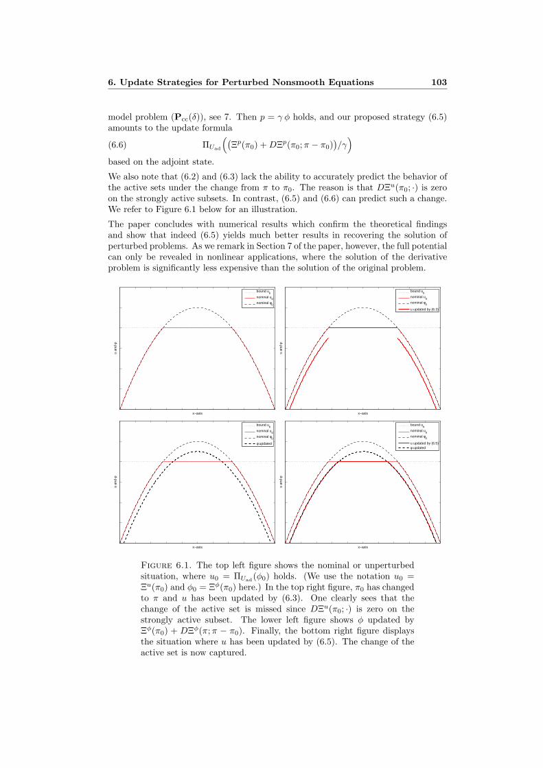
6. Update Strategies for Perturbed Nonsmooth Equations 103

model problem (Pcc(δ)), see 7. Then p = γ φ holds, and our proposed strategy (6.5)amounts to the update formula

(6.6) ΠUad

((Ξp(π0) +DΞp(π0;π − π0)

)/γ)

based on the adjoint state.

We also note that (6.2) and (6.3) lack the ability to accurately predict the behavior ofthe active sets under the change from π to π0. The reason is that DΞu(π0; ·) is zeroon the strongly active subsets. In contrast, (6.5) and (6.6) can predict such a change.We refer to Figure 6.1 below for an illustration.

The paper concludes with numerical results which confirm the theoretical findingsand show that indeed (6.5) yields much better results in recovering the solution ofperturbed problems. As we remark in Section 7 of the paper, however, the full potentialcan only be revealed in nonlinear applications, where the solution of the derivativeproblem is significantly less expensive than the solution of the original problem.

x−axis

u an

d φ

bound u

b

nominal u0

nominal φ0

x−axis

u an

d φ

bound u

b

nominal u0

nominal φ0

u updated by (6.3)

x−axis

u an

d φ

bound u

b

nominal u0

nominal φ0

φ updated

x−axis

u an

d φ

bound u

b

nominal u0

nominal φ0

u updated by (6.5)φ updated

Figure 6.1. The top left figure shows the nominal or unperturbedsituation, where u0 = ΠUad(φ0) holds. (We use the notation u0 =Ξu(π0) and φ0 = Ξφ(π0) here.) In the top right figure, π0 has changedto π and u has been updated by (6.3). One clearly sees that thechange of the active set is missed since DΞu(π0; ·) is zero on thestrongly active subset. The lower left figure shows φ updated byΞφ(π0) + DΞφ(π;π − π0). Finally, the bottom right figure displaysthe situation where u has been updated by (6.5). The change of theactive set is now captured.

UPDATE STRATEGIES FOR PERTURBED NONSMOOTHEQUATIONS

ROLAND GRIESSE, THOMAS GRUND AND DANIEL WACHSMUTH

Abstract. Nonsmooth operator equations in function spaces are considered,which depend on perturbation parameters. The nonsmoothness arises from aprojection onto an admissible interval. Lipschitz stability in L∞ and Bouliganddifferentiability in Lp of the parameter-to-solution map are derived. An adjointproblem is introduced for which Lipschitz stability and Bouligand differentiabilityin L∞ are obtained. Three different update strategies, which recover a perturbedfrom an unperturbed solution, are analyzed. They are based on Taylor expansionsof the primal and adjoint variables, where the latter admits error estimates in L∞.Numerical results are provided.

1. Introduction

In this work we consider nonsmooth operator equations of the form

u = Π[a,b](g(θ)−G(θ)u), (Oθ)

where the unknown u ∈ L2(D) is defined on some bounded domain D ⊂ RN , and θ isa parameter. Moreover, Π[a,b] denotes the pointwise projection onto the set

Uad = u ∈ L2(D) : a(x) ≤ u(x) ≤ b(x) a.e. on D.Such nonsmooth equations appear as a reformulation of the variational inequality

Find u ∈ Uad s.t. 〈u + G(θ)u − g(θ), v − u〉 ≥ 0 for all v ∈ Uad. (VIθ)

Applications of (VIθ) abound, and we mention in particular control-constrained opti-mal control problems.

Throughout, G(θ) : L2(D) → L2+δ(D) is a bounded and monotone linear operatorwith smoothing properties, such as a solution operator to a differential equation, andg(θ) ∈ L∞(D). Both G and g may depend nonlinearly and also in a nonsmooth wayon a parameter θ in some normed linear space Θ. Under conditions made precise inSection 2, (Oθ) has a unique solution u[θ] for any given θ. We are concerned herewith the behavior of u[θ] under perturbations of the parameter. In particular, weestablish the directional differentiability of the nonsmooth map u[·] with uniformlyvanishing remainder, a concept called Bouligand differentiability (B-differentiabilityfor short). We prove B-differentiability of u[·] : Θ → Lp(D) for p ∈ [1,∞), which isa sharp result and allows a Taylor expansion of u[·] around a reference parameter θ0

with error estimates in Lp(D).Based on this Taylor expansion, we analyze three update strategies

C1(θ) := u0 + u′[θ0](θ − θ0)

C2(θ) := Π[a,b]

(u0 + u′[θ0](θ − θ0)

)C3(θ) := Π[a,b]

(φ0 + φ′[θ0](θ − θ0)

)which allow to recover approximations of the perturbed solution u[θ] from the referencesolution u0 = u[θ0] and derivative information. Our main result is that (C3), which


involves a dual (adjoint) variable satisfying

φ = g(θ)−G(θ)Π[a,b]φ,

allows error estimates in L∞(D) while the other strategies do not. We thereforeadvocate to use update strategy (C3).

As an important application, our setting accomodates linear–quadratic optimalcontrol problems, where u is the control variable, S represents the control–to–state mapassociated to a linear elliptic or parabolic partial differential equation and G = S⋆S.Then (Oθ) are necessary and sufficient optimality conditions. We shall elaborate onthis case later on.

In the context of optimal control, B-differentiability of optimal solutions for semi-linear problems has been investigated in [4, 6]. We provide here a simplified proof inthe linear case.

The outline of the paper is as follows: In Section 2, we specify the problem settingand recall the concept of B-differentiability. In Sections 3 and 4, we prove the Lipschitzstability of the solution map u[·] into L∞(D) and its B-differentiability into Lp(D),p < ∞. Section 5 is devoted to the analysis of the adjoint problem, for which weprove B-differentiability into L∞(D). In Section 6, we discuss the application of thesemismooth Newton method to the original problem and the problem associated withthe derivative. We analyze the three update strategies (C1)–(C3) in Section 7 andprove error estimates. In Section 8 we apply our results to the optimal control of alinear elliptic partial differential equation and report on numerical results confirmingthe superiority of the adjoint-based strategy (C3).

Throughout, c and L denote generic positive constants which take different valuesin different locations.

2. Problem Setting

Let us specify the standing assumptions for problem (Oθ) taken to hold throughoutthe paper. We assume that D ⊂ RN is a bounded and measurable domain, N ≥ 1.By Lp(D), 1 ≤ p ≤ ∞, we denote the Lebuesge spaces of p-integrable or essentiallybounded functions on D. We write 〈u, v〉 to denote the scalar product of two functionsu, v ∈ L2(D). The norm in Lp(D) is denoted by ‖ · ‖p or simply ‖ · ‖ in the casep = 2. The space of bounded linear operators from Lp(D) to Lq(D) is denoted byL(Lp(D), Lq(D)) and its norm by ‖ · ‖p→q.

The lower and upper bounds a, b : D → [−∞,∞] for the admissible set are functionssatisfying a(x) ≤ b(x) a.e. on D. We assume the existence of an admissible functionu∞ ∈ L∞(D) ∩ Uad. Hence, the admissible set

Uad = u ∈ L2(D) : a(x) ≤ u(x) ≤ b(x) a.e. on Dis nonempty, convex and closed but not necessarily bounded in L2(D). Π[a,b] denotesthe pointwise projection of a function on D onto Uad, i.e.,

Π[a,b]u = maxa, minu, bpointwise on D. Note that Π[a,b] : Lp(D) → Lp(D) is Lipschitz continuous withLipschitz constant 1 for all p ∈ [1,∞].

Finally, let Θ be the normed linear space of parameters with norm ‖ · ‖ and letθ0 ∈ Θ be a given reference parameter. We recall two definitions:

Definition 2.1. A function f : X → Y is said to be locally Lipschitz continuous atx0 ∈ X if there exists an open neighborhood of x0 and L > 0 such that

‖f(x)− f(y)‖Y ≤ L‖x− y‖X

holds for all x, y in the said neighborhood of x0. In addition, f is said to be locallyLipschitz continuous if it is locally Lipschitz continuous at all x0 ∈ X.


Definition 2.2. A function f : X → Y between normed linear spaces X and Y issaid to be B-differentiable at x0 ∈ X if there exists ε > 0 and a positively homogeneousoperator f ′(x0) : X → Y such that

f(x) = f(x0) + f ′(x0)(x− x0) + r(x0; x− x0)

holds for all x ∈ X, where the remainder satisfies ‖r(x0; x− x0)‖Y /‖x− x0‖X → 0 as‖x− x0‖X → 0. In addition, f is said to be B-differentiable if it is B-differentiable atall x0 ∈ X.

The B-derivative is also called a directional Frechet derivative, see [1]. Recall thatan operator A : X → Y is said to be positively homogeneous if A(λx) = λA(x) holdsfor all λ ≥ 0 and all x ∈ X .

Let us specify the standing assumptions for the function g:

(1) g is locally Lipschitz continuous from Θ to L∞(D)(2) g is B-differentiable from Θ to L∞(D).

Moreover, we assume that G : Θ → L(L2(D), L2(D)) satisfies the following smoothingproperties with some δ > 0:

(3) G(θ) is bounded from Lp(D) to Lp+δ(D) for all p ∈ [2,∞) and all θ ∈ Θ(4) G(θ) is bounded from Lp(D) to L∞(D) for all p > p0 and all θ ∈ Θ.

In addition, we demand that G(θ) : L2(D) → L2(D) is monotone for all θ ∈ Θ:

〈G(θ)(u − v), u − v〉 ≥ 0 for all u, v ∈ L2(D),

and that

(5) G is locally Lipschitz continuous from Θ to L(L2(D), L2(D))(6) G is locally Lipschitz continuous from Θ to L(L∞(D), L∞(D)).

Finally, we assume that

(7) G is B-differentiable from Θ to L(Lp0+δ(D), L∞(D)).

Remark 2.3. For control-constrained optimal control problems, G = S⋆S where S isthe solution operator of the differential equation involved. An example is presented inSection 8. If assumptions (1)–(2) and (5)–(7) hold only at a specified parameter θ0

and (3)–(4) hold only in a neighborhood of θ0, the subsequent analysis remains validlocally.

Remark 2.4. The assumptions (1)–(7) can be changed if G does not map into L∞(D)but only into Ls(D) for some s ∈ (2,∞).

(1’) g is locally Lipschitz continuous from Θ to Ls(D)(2’) g is B-differentiable from Θ to Ls(D).(3’) G(θ) is bounded from Lp(D) to Lp+δ(D) for all p ∈ [2, s− δ] and all θ ∈ Θ(5’) G is locally Lipschitz continuous from Θ to L(L2(D), L2(D))(6’) G is locally Lipschitz continuous from Θ to L(Ls(D), Ls(D)).(7’) G is B-differentiable from Θ to L(Ls(D), Ls(D)).

In this case, the results of Proposition 3.2 and Theorems 4.5 and 5.2 change accord-ingly. In particular, our main result Theorem 7.1 remains true if ∞ is replaced bys.

In the sequel, we will need the B-derivative of a composite function. A similar resultfor a related differentiation concept can be found in [8, Prop. 3.6].

Lemma 2.5. Consider normed linear spaces X, Y, Z and mappings F : Y → Z,G : X → Y . Assume that the mapping G is B-differentiable at θ0 ∈ X and that F is B-differentiable at G(θ0). Furthermore assume that G is locally Lipschitz continuous at θ0


and that F ′(G(θ0)) is locally Lipschitz continuous at 0. Then the mapping H : X → Zdefined by H = F G is B-differentiable at θ0 with the derivative

H ′(θ0) = F ′(G(θ0)) G′(θ0).

Proof. Applying B-differentiability of F and G we obtain

F (G(θ)) − F (G(θ0)) = F ′(G(θ0)) (G(θ)−G(θ0)) + rF ,

= F ′(G(θ0)) (G′(θ0)(θ − θ0) + rG) + rF

(2.1)

with the remainder terms rF and rG satisfying‖rF ‖Z

‖G(θ)−G(θ0)‖Y→ 0 as ‖G(θ)−G(θ0)‖Y → 0

and‖rG‖Y

‖θ − θ0‖X→ 0 as ‖θ − θ0‖X → 0

respectively. Now let us write

F ′(G(θ0)) (G′(θ0)(θ − θ0) + rG) = F ′(G(θ0))G′(θ0)(θ − θ0)

+ F ′(G(θ0)) (G′(θ0)(θ − θ0) + rG)− F ′(G(θ0))G′(θ0)(θ − θ0). (2.2)

Putting (2.1) and (2.2) together, we get an expression for the remainder term

F (G(θ)) − F (G(θ0))− F ′(G(θ0))G′(θ0)(θ − θ0)

= rF + F ′(G(θ0)) (G′(θ0)(θ − θ0) + rG)− F ′(G(θ0))G′(θ0)(θ − θ0) (2.3)

Note that G′(θ0)(θ−θ0) and rG are small in the norm of Y whenever θ−θ0 is small inthe norm of X . Since F ′(G(θ0)) is locally Lipschitz continuous at 0, we can estimate

‖F (G(θ))− F (G(θ0))− F ′(G(θ0))G′(θ0)(θ − θ0)‖Z ≤ ‖rF ‖Z + cF ′‖rG‖Y .

It remains to prove that the right-hand side, divided by ‖θ − θ0‖X , vanishes for ‖θ −θ0‖X → 0. This is true for ‖rG‖Y . So we have to investigate ‖rF ‖Z :

‖rF ‖Z

‖θ − θ0‖X=

‖rF ‖Z

‖G(θ)−G(θ0)‖Y

‖G(θ)−G(θ0)‖Y

‖θ − θ0‖X≤ cG

‖rF ‖Z

‖G(θ)−G(θ0)‖Y

by the local Lipschitz continuity of G at θ0. For ‖θ − θ0‖X → 0 it follows ‖G(θ) −G(θ0)‖Y → 0. Hence, the right-hand side vanishes for ‖θ − θ0‖X → 0. And the proofis complete.

Combining locally Lipschitz continuity and B-differentiability, we can prove a usefulcontinuity result for the B-derivative.

Lemma 2.6. Consider normed linear spaces X, Y and the mapping G : X → Y .Let G be B-differentiable and locally Lipschitz continuous at θ0 ∈ X. Then it holds‖G′(θ0)(θ − θ0)‖Y → 0 for ‖θ − θ0‖X → 0, i.e. the B-derivative is continuous in theorigin with respect to the direction.

Proof. By local Lipschitz continuity of G at θ0, there exist ǫ > 0 and L > 0 such that

‖G(θ)−G(θ0)‖Y ≤ L‖θ − θ0‖X ∀θ ∈ X : ‖θ − θ0‖X < ǫ.

Let us writeG(θ) = G(θ0) + G′(θ0)(θ − θ0) + rG

with the remainder rG satisfying‖rG‖Y

‖θ − θ0‖X→ 0 as ‖θ − θ0‖X → 0.

Then, we have‖G′(θ0)(θ − θ0)‖Y ≤ L‖θ − θ0‖X + ‖rG‖Y ,


and it follows that the right-hand side tends to zero as ‖θ − θ0‖X → 0.

3. Lipschitz Stability of the Solution Map

In this section we draw some simple conclusions from the assumptions made inSection 2. We recall that our problem (Oθ) is equivalent to the following variationalinequality:

Find u ∈ Uad s.t. 〈u + G(θ)u − g(θ), v − u〉 ≥ 0 for all v ∈ Uad. (VIθ)

We begin by proving the Lipschitz stability of solutions u[θ] with respect to the L2(D)norm.

Lemma 3.1. For any given θ ∈ Θ, (Oθ) has a unique solution u[θ] ∈ L2(D). Thesolution map u[·] is locally Lipschitz continuous from Θ to L2(D).

Proof. Let θ ∈ Θ be given and let F (u) = u + G(θ)u− g(θ). By monotonicity of G(θ)it follows that 〈F (u1)− F (u2), u1 − u2〉 ≥ ‖u1 − u2‖2, hence F is strongly monotone.This implies the unique solvability of (VIθ) and thus of (Oθ), see, for instance, [3].

If θ′ ∈ Θ is another parameter, then we obtain from (VIθ)

〈u + G(θ)u − g(θ), u′ − u〉+ 〈u′ + G(θ′)u′ − g(θ′), u − u′〉 ≥ 0.

Inserting the term G(θ′)u−G(θ′)u and using the monotonicity of G(θ′), we obtain

‖u′ − u‖2 ≤ (‖G(θ)−G(θ′)‖2→2‖u‖+ ‖g(θ)− g(θ′)‖) ‖u′ − u‖.

This proves the local Lipschitz continuity of u[·] at any given parameter θ: Supposethat θ and θ′ are in some ball of radius ε around θ0 such that, by Assumption (5),‖G(θ)−G(θ′)‖2→2 ≤ L‖θ−θ′‖. If we set u0 = u[θ0], then ‖u−u0‖ ≤ L‖θ−θ0‖‖u0‖ ≤εL‖u0‖ and thus ‖u‖ ≤ εL‖u0‖+ ‖u0‖. Hence ‖u′− u‖ ≤ L‖θ− θ′‖(1 + εL)‖u0‖.

By exploiting the smoothing properties of G(θ), this result can be strenghtened:

Proposition 3.2. The solution map u[·] is locally Lipschitz continuous from Θ toL∞(D).

Proof. We use a bootstrapping argument to show that the solution u[θ] lies in L∞(D).The fact that g(θ) ∈ L∞(D) and the smoothing property (3) of G(θ) yield g(θ) −G(θ)u[θ] ∈ L2+δ(D). By the properties of the projection, it follows from (Oθ) thatu[θ] ∈ L2+δ(D). Repeating this argument until 2 + nδ > p0, we find u[θ] ∈ L∞(D) byAssumption (4).

We prove without loss of generality the local Lipschitz continuity of u[·] at thereference parameter θ0. Let θ and θ′ be any two parameters in a ball of radius εaround θ0 such that ‖G(θ)−G(θ′)‖∞→∞ ≤ L‖θ−θ′‖ and ‖g(θ)−g(θ′)‖∞ ≤ L‖θ−θ′‖hold. Using the Lipschitz continuity of the projection, we obtain

‖u− u′‖2+δ ≤ ‖g(θ)− g(θ′)‖2+δ + ‖G(θ)u −G(θ′)u′‖2+δ

≤ c ‖g(θ)− g(θ′)‖∞ + ‖G(θ)(u − u′)‖2+δ + ‖(G(θ)−G(θ′))u′‖2+δ

≤ c L ‖θ− θ′‖+ c ‖u− u′‖+ c L ‖θ− θ′‖‖u′‖∞for some c > 0 and hence the local Lipschitz stability for u[·] in L2+δ(D) follows.Repeating this argument until 2 + nδ > p0, we obtain the local Lipschitz stability foru[·] in L∞(D).


4. B-Differentiability of the Solution Map

In this section we study the differentiability properties of the solution map u[·],which depend on the properties of the projection. We extend the results of [5]. Let usdefine a set I[a, b, u0] by

I[a, b, u0] =

u ∈ L2(D) :

u(x) = 0 u0(x) 6∈ [a(x), b(x)]u(x) = 0 if u0(x) = a(x) = b(x)u(x) ≥ 0 u0(x) = a(x)u(x) ≤ 0 u0(x) = b(x)

.

The pointwise projection on this set is denoted by ΠI[a,b,u0]. By construction it holdsfor u0, u, a, b ∈ L2(D), a ≤ b

ΠI[a,b,u0](u) = −ΠI[−b,−a,−u0](−u),

ΠI[a,+∞,u0](u) = ΠI[0,+∞,u0−a](u),

ΠI[a,b,u0](u) = ΠI[a,+∞,u0]

(ΠI[−∞,b,u0](u)

).

(4.1)

It turns out that ΠI[a,b,u0] is the B-derivative of the projection onto the admissibleset Π[a,b]. We start with the proof of B-differentiability of the projection on the coneof non-negative functions.

Theorem 4.1. The projection Π[0,+∞] is B-differentiable from Lp(D) to Lq(D) for1 ≤ q < p ≤ ∞. And it holds

Π[0,+∞](u) = Π[0,+∞](u0) + ΠI[0,+∞,u0](u − u0) + r1 (4.2a)

where‖r1‖q

‖u− u0‖p→ 0 as ‖u− u0‖p → 0. (4.2b)

Remark 4.2. The claim for the case p = ∞ was proven in [5]. A counterexamplewas given there, which shows that the projection is not B-differentiable from L∞(D)to L∞(D).

Proof of Theorem 4.1. Clearly, the function ΠI[0,+∞,u0] is positively homogeneous.Let us define the function r as the remainder term

r = Π[0,+∞](u)−Π[0,+∞](u0)−ΠI[0,+∞,u0](u− u0). (4.3)

A short calculation shows that

r(x) =

|u(x)| if u(x)u0(x) < 00 otherwise

(4.4)

holds, see also the discussion in [5]. It implies the estimate r(x) ≤ |u(x)−u0(x)|. Nowsuppose that 1 ≤ q < p ≤ ∞. It remains to prove

‖r‖q

‖u− u0‖p→ 0 as ‖u− u0‖p → 0. (4.5)

We will argue by contradiction. Assume that (4.5) does not hold. Then there existsǫ > 0 such that for all δ > 0 there is a function uδ with ‖uδ − u0‖p < δ and satisfying

‖rδ‖q

‖uδ − u0‖p≥ ǫ. (4.6)

Here, rδ is the remainder term defined as in (4.3). Let us choose a sequence δk withlimk→∞ δk = 0, uk = uδk

, and rk := rδk. By Egoroff’s Theorem, for each σ > 0 there


exists a set Dσ ⊂ D with meas(D \ Dσ) < σ such that the convergence uk → u0 isuniform on Dσ. It allows us to estimate

‖rk‖q ≤(∫

D\Dσ

|uk(x) − u0(x)|qdx

)1/q

+(∫

Dσ

|rk(x)|qdx

)1/q

≤ σ1q− 1

p ‖uk − u0‖p +(∫

Dσ

|rk(x)|qdx

)1/q

.

Here, the second addend needs more investigation. Let us define a subset Dσ,k of Dσ

by

Dσ,k =

x ∈ Dσ : 0 < |u0(x)| < supx′∈Dσ

|uk(x′)− u0(x′)|

.

Then by construction it holds rk(x) = 0 on Dσ \ Dσ,k, compare (4.4). Observe thatmeas(Dσ,k) → 0 as k → ∞ due to the uniform convergence of uk to u0 on Dσ. Andwe can proceed with

‖rk‖q ≤ σ1q− 1

p ‖uk − u0‖p +(∫

Dσ

|rk(x)|qdx

)1/q

= σ1q− 1

p ‖uk − u0‖p +

(∫Dσ,k

|rk(x)|qdx

)1/q

≤ σ1q− 1

p ‖uk − u0‖p + meas(Dσ,k)1q− 1

p ‖uk − u0‖p,

which is a contradiction to (4.6).

Now, we calculate the B-derivative of Π[a,b] using the chain rule developed inLemma 2.5.

Theorem 4.3. The projection Π[a,b] is B-differentiable from Lp(D) to Lq(D) for1 ≤ q < p ≤ ∞. And it holds

Π[a,b](u) = Π[a,b](u0) + ΠI[a,b,u0](u− u0) + r1 (4.7a)

where‖r1‖q

‖u− u0‖p→ 0 as ‖u− u0‖p → 0. (4.7b)

Proof. The projection Π[a,b] can be written as a composition of two projections on theset of non-negative functions as

Π[a,b](u) = Π[0,+∞]

(b−Π[0,+∞](b− u)− a

)+ a.

The projection Π[0,+∞] and its B-derivative ΠI[0,+∞,u0] are Lipschitz continuous.Thus, the B-differentiability of Π[a,b] follows by Lemma 2.5.

The chain rule yields the derivative

Π′[a,b](u0)(u − u0) = ΠI[0,+∞,b−Π[0,+∞](b−u0)−a]

(−ΠI[0,+∞,b−u0](−(u− u0)))

= ΠI[0,+∞,b−Π[0,+∞](b−u0)−a]

(ΠI[−∞,b,u0](u− u0)

)= ΠI[a,+∞,Π[−∞,b](u0)]

(ΠI[−∞,b,u0](u− u0)

).

Here, we used the properties (4.1) of the projection ΠI . It remains to prove that theright-hand side is equal to ΠI[a,b,u0](u−u0). To this end, let us introduce the followingdisjoint subsets of D:

D1 := x ∈ D : u0(x) ≤ b(x),D2 := x ∈ D : b(x) < u0(x).


Let us denote by χDi the characteristic function of the set Di. The projection ΠI isadditive with respect to functions with disjoint support, i.e.

ΠI[a,b,u0](v) = ΠI[a,b,u0](χD1v) + ΠI[a,b,u0](χD2v)

holds for all a, b, u0, v. Since Π′[a,b](u0)(u − u0) is a composition of such projections,

we can split

Π′[a,b](u0)(u − u0) = Π′

[a,b](u0)(χD1(u− u0)) + Π′[a,b](u0)(χD2(u − u0)).

Furthermore, it holds ΠI[a,b,u0](χDiv) = ΠI[a,b,χDiu0](χDiv). At first, we have

χD1Π[−∞,b](χD1u0) = χD1u0.

Π′[a,b](u0)(χD1(u− u0)) = ΠI[a,+∞,Π[−∞,b](u0)]

(ΠI[−∞,b,u0](χD1(u− u0))

)= ΠI[a,+∞,u0]

(ΠI[−∞,b,u0](χD1(u− u0))

)= ΠI[a,b,u0](χD1(u− u0)).

The last equality follows from the third property of ΠI in (4.1).For the second set D2, we have

ΠI[−∞,b,u0](χD2(u− u0)) = 0,

since u0(x) is not admissible for x ∈ D2. For the same reason, we get also

ΠI[a,b,u0](χD2(u− u0)) = 0,

which gives

Π′[a,b](u0)(χD2 (u− u0)) = 0 = ΠI[a,b,u0](χD2(u − u0)).

Consequently, we obtain

Π′[a,b](u0)(u− u0) = Π′

[a,b](u0)(χD1(u − u0)) + Π′[a,b](u0)(χD2(u− u0))

= ΠI[a,b,u0](χD1(u − u0)) + ΠI[a,b,u0](χD2(u− u0))

= ΠI[a,b,u0](u − u0),

and the claim is proven.

Let us remark that the result of the last two Theorems is sharp with respect to thechoice of function spaces:

Remark 4.4. The projection is not B-differentiable from Lp(D) to Lp(D) for anyp, as the following example shows. Take a = 0, b = +∞, D = (0, 1). We chooseu0(x) = −1 and

uk(x) =

1 if x ∈ (0, 1/k)−1 otherwise.

In this case, the remainder term given by (4.4) is r1,k = (uk − u0)/2. Therefore itholds

‖r1,k‖p

‖uk − u0‖p=

126→ 0 for k →∞.

As a side result of the previous theorem, however, we get for α ∈ (−∞, 1)

‖r1,k‖p

‖uk − u0‖αp

→ 0 for k →∞.

We are now in the position to prove B-differentiability of the solution mapping u[θ]of our non-smooth equation (Oθ).


Theorem 4.5. The solution mapping u[θ] of problem (Oθ) is B-differentiable from Θto Lp(D), 2 ≤ p < ∞. The Bouligand derivative of u[·] at θ0 in direction θ, henceforthcalled u′[θ0]θ, is the unique solution of the non-smooth equation

u = ΠI[a,b,φ0](g′(θ0)θ −G(θ0)u− (G′(θ0)θ)u0) (O′

θ0;θ)

where u0 = u[θ0] and φ0 = g(θ0)−G(θ0)u0.

Proof. The problem (O′θ0;θ

) is equivalent to finding a solution u ∈ I[a, b, φ0] of thevariational inequality

〈u + G(θ0)u + (G′(θ0)θ)u0 − g′(θ0)θ, v − u〉 ≥ 0 ∀v ∈ I[a, b, φ0].

By monotonicity of G(θ0) this variational inequality is uniquely solvable, compareLemma 3.1. Moreover, the projection ΠI[a,b,φ0] is positively homogeneous. So themapping θ 7→ u′[θ0]θ is positively homogeneous as well.

Now, let us take θ1 ∈ Θ and u1 := u[θ1]. Let p ∈ [2,∞) be fixed. Further, let ud

be the solution of (O′θ0;θ

) for θ = θ1 − θ0, i.e.

ud = ΠI[a,b,φ0](g′(θ0)(θ1 − θ0)−G(θ0)ud −G′(θ0)(θ1 − θ0)u0). (4.8)

Let us investigate the difference u1 − u0. We obtain by B-differentiability of theprojection from Lp+δ(D) to Lp(D)

u1 − u0 = Π[a,b](g(θ1)−G(θ1)u1)−Π[a,b](g(θ0)−G(θ0)u0)

= ΠI[a,b,g(θ0)−G(θ0)u0](g(θ1)−G(θ1)u1 − g(θ0) + G(θ0)u0) + r1

= ΠI[a,b,φ0](g(θ1)−G(θ1)u1 − g(θ0) + G(θ0)u0) + r1.

(4.9)

The remainder term r1 satisfies‖r1‖p

‖g(θ1)−G(θ1)u1 − g(θ0) + G(θ0)u0‖p+δ→ 0

as ‖g(θ1)−G(θ1)u1− g(θ0)+ G(θ0)u0‖p+δ → 0. Applying Lipschitz continuity of u[·],G, and g, we get

‖g(θ1)−G(θ1)u1 − g(θ0) + G(θ0)u0‖p+δ ≤ c (‖θ1 − θ0‖+ ‖u1 − u0‖p)

≤ c ‖θ1 − θ0‖.Hence, we find for the remainder term

‖r1‖p

‖θ1 − θ0‖ → 0 as ‖θ1 − θ0‖ → 0. (4.10)

Let us rewrite (4.9) as

u1 − u0 − r1 = ΠI[a,b,φ0]

(g(θ1)− g(θ0)−G(θ0)(u1 − u0)− (G(θ1)−G(θ0))u1

)= ΠI[a,b,φ0]

(g′(θ0)(θ1 − θ0) + rg

1 −G(θ0)(u1 − u0)

− (G′(θ0)(θ1 − θ0) + rG1 )u1

)= ΠI[a,b,φ0]

(g′(θ0)(θ1 − θ0)−G(θ0)(u1 − u0 − r1)

−G′(θ0)(θ1 − θ0)u1 + rg1 + rG

1 u1 −G(θ0)r1

)= ΠI[a,b,φ0]

(g′(θ0)(θ1 − θ0)−G(θ0)(u1 − u0 − r1)

−G′(θ0)(θ1 − θ0)u1 + r∗1)

with a remainder term r∗1 = rg1 + rG

1 u1 −G(θ0)r1 satisfying

‖r∗1‖p

‖θ1 − θ0‖ → 0 as ‖θ1 − θ0‖ → 0. (4.11)

We can interpret ur := u1 − u0 − r1 as the solution of the non-smooth equation

ur = ΠI[a,b,φ0]

(g′(θ0)(θ1 − θ0)−G(θ0)ur −G′(θ0)(θ1 − θ0)u1 + r∗1

),


which is similar to (4.8) but perturbed by −G′(θ0)(θ1 − θ0)(u1 − u0) + r∗1 . Analo-gously as in Section 3, it can be shown that the solution mapping of that equationis Lipschitz continuous in the data, i.e., the map r ∋ Lp(D) 7→ u ∈ Lp(D), whereu = ΠI[a,b,φ0](−G(θ0)u + r), is Lipschitz continuous.

So we can estimate

‖u1 − u0 − r1 − ud‖p = ‖ur − ud‖p ≤ c ‖G′(θ0)(θ1 − θ0)(u1 − u0)‖p + c ‖r∗1‖p

≤ c ‖G′(θ0)(θ1 − θ0)(u1 − u0)‖∞ + c ‖r∗1‖p. (4.12)

Using the assumptions on G, we obtain by Lemma 2.6

‖G′(θ0)(θ1 − θ0)‖∞→∞ → 0 as ‖θ1 − θ0‖ → 0.

The mapping θ 7→ u[θ] is locally Lipschitz continuous from Θ to L∞(D), see Proposi-tion 3.2. Both properties imply

‖G′(θ0)(θ1 − θ0)(u1 − u0)‖∞‖θ1 − θ0‖ → 0 as ‖θ1 − θ0‖ → 0. (4.13)

Combining (4.11)–(4.13) yields in turn

‖u1 − u0 − r1 − ud‖p

‖θ1 − θ0‖ → 0 as ‖θ1 − θ0‖ → 0. (4.14)

Finally, we have

‖u1 − (u0 + ud)‖p ≤ ‖u1 − u0 − r1 − ud‖p + ‖r1‖p

and consequently by (4.10) and (4.14)

‖u1 − (u0 + ud)‖p

‖θ1 − θ0‖ → 0 as ‖θ1 − θ0‖ → 0. (4.15)

Hence, ud is the Bouligand derivative of u[·] at θ0 in the direction θ1 − θ0.

Remark 4.6. This result cannot be strengthened. The map u[θ] cannot be Bouligandfrom Θ to L∞(D). To see this, consider the case G = 0. It trivially fulfills allrequirements of Section 2. Then u[θ] = Π[a,b](g(θ)) holds, but the projection Π[a,b] isnot B-differentiable from L∞(D) to L∞(D), see Remark 4.4.

Lemma 4.7. The B-derivative u′[θ0] satisfies for all α ∈ (−∞, 1)

‖u[θ0] + u′[θ0](θ1 − θ0)− u[θ1]‖∞‖θ1 − θ0‖α

→ 0 as ‖θ1 − θ0‖ → 0.

Proof. Here, we will follow the steps of the proof of the previous theorem. Let α beless than 1. The limiting factors in the proof are the remainder terms r1 and r∗1 . Weobtain for r1 and r∗1 due to Remark 4.4 the property

‖r1‖∞‖θ1 − θ0‖α

→ 0 and‖r∗1‖∞

‖θ1 − θ0‖α→ 0 as ‖θ1 − θ0‖ → 0.

Combining these with estimates (4.12)–(4.15) completes the proof.

5. Properties of the Adjoint Problem

In this section we investigate an adjoint problem defined by

φ = g(θ)−G(θ)Π[a,b](φ). (Dθ)

If we interpret (Oθ) as an optimal control problem with control constraints, see Sec-tion 8, then problem (Dθ) is an equation for the adjoint state. The primal and adjointformulations are closely connected: If u[θ] is the unique solution of (Oθ) then

φ := g(θ)−G(θ)u[θ] (5.1)


is a solution of (Dθ), which means that (Dθ) admits at least one solution. And if φ isa solution of the dual (adjoint) equation (Dθ) then the projection u = Π[a,b](φ[θ]) isthe unique solution of the original problem (Oθ).

Now, let us briefly answer the question of uniqueness of adjoint solutions. If φ1 andφ2 are two solutions of (Dθ), then both Π[a,b](φ1) and Π[a,b](φ2) are solutions of (Oθ).By Lemma 3.1 this problem has a unique solution, hence Π[a,b](φ1) = Π[a,b](φ2). Forthe difference φ1 − φ2 we have

φ1 − φ2 = g(θ)−G(θ)Π[a,b](φ1)−(g(θ)−G(θ)Π[a,b](φ2)

)= −G(θ)(Π[a,b](φ1)−Π[a,b](φ2)) = 0,

which implies in fact the unique solvability of (Dθ). In the following, we denote thisunique solution by φ[θ]. An immediate conclusion of the considerations in Section 3is the Lipschitz property of φ[·].Corollary 5.1. The mapping φ[θ] is locally Lipschitz from Θ to L∞(D).

Thus, we found that φ[·] inherits Lipschitz continuity from u[·]. However, in contrastto the primal map u[·], the adjoint map φ[·] is B-differentiable into L∞(D). Theproperty which allows us to prove this result is that in (Dθ), the smoothing operatorG(θ) is applied after the projection Π[a,b].

Theorem 5.2. The mapping φ[θ] is B-differentiable from Θ to L∞(D). The B-derivative of φ[·] at θ0 in direction θ, henceforth called φ′[θ0]θ, is the solution of thenon-smooth equation

φ = g′(θ0)θ −G(θ0)ΠI[a,b,φ0](φ) − (G′(θ0)θ)Π[a,b](φ0), (5.2)

where φ0 = φ[θ0] = g(θ0)−G(θ0)u[θ0].

Proof. Due to the linearity of G, the B-derivative of H(θ) := G(θ)u[θ] at θ0, in thedirection of θ, can be written as

H ′(θ0)θ = G(θ0)u′[θ0]θ + (G′(θ0)θ)u0,

where u0 = u[θ0]. By Theorem 4.5, u[·] is B-differentiable from Θ to Lp0+δ(D).Together with the B-differentiability of G(·) from Θ to L(Lp0+δ(D), L∞(D)), the re-lationship φ[θ] = g(θ) −G(θ)u[θ] implies B-differentiability of φ[·] from Θ to L∞(D).The formula (5.2) is obtained by differentiating equation (Dθ).

We now discuss the use of the derivative of φ[θ] to obtain an update rule for theprimal variable u[θ]. Suppose that u0 = u[θ0] and φ0 = φ[θ0] are the solutions ofthe primal and dual problems at the reference parameter θ0. We use the followingconstruction as a first-order approximation of u[θ]:

u[θ0, θ − θ0] := C3(θ) = Π[a,b]

(φ0 + φ′[θ0](θ − θ0)

). (5.3)

We can prove that the L∞-norm of the remainder u[θ] − u[θ0, θ − θ0], divided by‖θ − θ0‖, vanishes as θ → θ0. This is a stronger result than can be obtained usingmerely the B-differentiability. There, the remainder u[θ]−u[θ0]−u′[θ0](θ−θ0), dividedby ‖θ−θ0‖, vanishes only in weaker Lp-norms. We refer to Section 7 for a comparisonof this advanced update rule with the conventional rules (C1) and (C2).

Corollary 5.3. Let u[θ0, θ − θ0] be given by (5.3). Then

‖u[θ]− u[θ0, θ − θ0]‖∞‖θ − θ0‖ → 0 as θ → θ0.

Proof. By construction, we have

u[θ]− u[θ0, θ − θ0] = Π[a,b](φ[θ]) −Π[a,b]

(φ[θ0] + φ′[θ0](θ − θ0)

).


The projection is Lipschitz from L∞(D) to L∞(D), hence we can estimate

‖u[θ]− u[θ0, θ − θ0]‖∞ ≤ ‖φ[θ]− φ[θ0]− φ′[θ0](θ − θ0)‖∞.

We know already by Theorem 5.2 that φ[θ] is B-differentiable at θ0 from Θ to L∞(D).Thus, it holds for ‖θ − θ0‖ → 0

‖φ[θ]− φ[θ0] + φ′[θ0](θ − θ0)‖∞‖θ − θ0‖ → 0.

for θ − θ0 → 0. Consequently, we get the same behavior for the remainder u[θ] −u[θ0, θ − θ0], which proves the claim.

In the next section we discuss how the quantities u[θ0], φ[θ0] and the requireddirectional derivatives of these quantities can be computed. It turns out that thederivative φ′[θ0](θ−θ0) is available at no additional cost when evaluating u′[θ0](θ−θ0),so the new update rule (C3) incurs no additional cost.

On the other hand, it is also easily possible to obtain φ′[θ0](θ−θ0) a posteriori fromu′[θ0](θ − θ0). Once u′[θ0](θ − θ0) is known, φ′[θ0](θ − θ0) can be computed from

φ′[θ0](θ − θ0) = g′(θ0)(θ − θ0)−G(θ0)u′[θ0](θ − θ0)− (G′(θ0)(θ − θ0))u0.

Hence the a posteriori computation of φ′ involves only the application of G and G′

and it is not necessary to solve any additional non-smooth equations. For optimalcontrol problems the quantity φ′[θ0](θ − θ0) is closely related to the adjoint state ofthe problem belonging to u′[θ0](θ − θ0).

6. Computation of the Solution and its Derivative

In this section we address the question how to solve problem (Oθ) for the nominalparameter θ0 and the derivative problem (O′

θ0;θ) algorithmically. In the recent past,generalized Newton methods in function spaces have been developed [2, 10], where ageneralized set-valued derivative plays the role of the Frechet derivative in the classicalNewton method. The semismooth Newton concept can be applied here, in view of thesmoothing properties of the operator G(θ0).

Let us consider the following nonsmooth equation:

F (u) := −u + g(θ0)−G(θ0)u−max0, g(θ0)−G(θ0)u − b−min0, g(θ0)−G(θ0)u− a = 0. (6.1)

It is easy to check that (6.1) holds if and only if u solves (Oθ) at θ0.Following [2], we infer that F is Newton differentiable as a map from Lp(D) to

Lp(D) for any p ∈ [2,∞]. The usual norm gap in the min and max functions iscompensated by the smoothing properties of G(θ0). The generalized derivative of Fis set-valued, and we take

F ′(u) δu = −G(θ0) δu− δu + χA+(u)G(θ0) δu + χA−(u)G(θ0) δu

as a particular choice. Here,

A+(u) = x ∈ D : g(θ0)−G(θ0)u− b ≥ 0 A(u) = A+(u) ∪A−(u)

A−(u) = x ∈ D : g(θ0)−G(θ0)u− a ≤ 0 I(u) = D \ A(u)

are the so-called active and inactive sets, and χA is the characteristic function of ameasurable set A. A generalized Newton step F ′(u) δu = −F (u) can be computed


by splitting the unknown δu into its parts supported on the active and inactive sets.Then a simple calculation shows that

on A+(u) : δu|A+(u) = b− u

on A−(u) : δu|A−(u) = a− u

on I(u) : (G(θ0) + I) δu|I(u) = g(θ0)−G(θ0)u− u−G(θ0) δu|A(u).

Lemma 6.1. For given u ∈ Lp(D) where 2 ≤ p ≤ ∞, the generalized Newton stepF ′(u) δu = −F (u) has a unique solution δu ∈ Lp(D).

Proof. We only need to verify that the step on the inactive set I(u) is indeed uniquelysolvable. This follows from the strong monotonicity of G(θ0) + I, considered as anoperator from L2(I(u)) to itself, compare the proof of Lemma 3.1. Hence the uniquesolution has an a priori regularity δu ∈ L2(D). The terms of lowest regularity on theright hand sides are the terms −u. Hence δu inherits the Lp(D) regularity of u. Notethat in case b or a are equal to ±∞ on a subset of D, this subset can not intersectA+(u) or A−(u) and thus the update δu lies in L∞(D), provided that u ∈ L∞(D),even if the bounds take on infinite values.

By the previous lemma, the generalized Newton iteration is well-defined. For aconvergence analysis, we refer to [2, 10]. For completeness, we state the semismoothNewton method for problem (Oθ) below (Algorithm 1). Note that the dual variable

Algorithm 1 Semismooth Newton algorithm to compute u0 and φ0.

1: Choose u0 ∈ L∞(D) and set n := 02: Set φn := g(θ0)−G(θ0)un

3: Set rn := F (un) = φn − un −max0, φn − b −min0, φn − a4: while ‖rn‖∞ > tol do5: Set δu|A+(un) := b− un on A+(un)6: Set δu|A−(un) := a− un on A−(un)7: Solve (G(θ0) + I) δu|I(un) = φn − un −G(θ0)δu|A(un) on I(un)8: Set un+1 := un + δu9: Set φn+1 := g(θ0)−G(θ0)un+1

10: Set rn+1 := F (un+1) = φn+1 − un+1 −max0, φn+1 − b −min0, φn+1 − a11: Set n := n + 112: end while13: Set u0 := un and φ0 := φn

φ0 appears naturally as an auxiliary quantity in the iteration, so it is available at noextra cost. With minor modifications, the same routine solves the derivative problems(O′

θ0;θ) for u′[θ0](θ) and (5.2) for φ′[θ0](θ) simultaneously. Similarly as before, we

consider the nonsmooth equation

F (u) := −u + g′(θ0)θ −G(θ0)u − (G′(θ0)θ)u0

−max0, g′(θ0)θ −G(θ0)u− (G′(θ0)θ)u0 − b−min0, g′(θ0)θ −G(θ0)u − (G′(θ0)θ)u0 − a = 0. (6.2)

Hats indicate variables that are associated with derivatives. The new bounds a andb depend on the solution and adjoint solution u0 and φ0 of the reference problem,through the definition of I[a, b, φ0] in Section 4:

a =

0 where u0 = a or φ0 6∈ [a, b]−∞ elsewhere

b =

0 where u0 = b or φ0 6∈ [a, b]∞ elsewhere.

(6.3)


The active and inactive sets A+(u) etc. for the derivative problem are taken withrespect to the bounds a and b. For the ease of reference, we also state the semis-mooth Newton method for the derivative problems u = u′[θ0]θ and φ = φ′[θ0]θ, seeAlgorithm 2. Note that these quantities satisfy

u′[θ0](θ) = ΠI[a,b,φ0]φ′[θ0]θ

φ′[θ0](θ) = g′(θ0)θ −G(θ0)u′[θ0]θ − (G′(θ0)θ)u0,

so each can be computed from the other.

Algorithm 2 Semismooth Newton algorithm to compute u′[θ0]θ and φ′[θ0]θ.

1: Choose u0 ∈ L∞(D) and set n := 02: Set the bounds a and b according to (6.3)3: Set φn := g′(θ0)θ −G(θ0)un − (G′(θ0)θ)u0

4: Set rn := F (un) = φn − un −max0, φn − b −min0, φn − a5: while ‖rn‖∞ > tol do6: Set δu| bA+(bun) := b− un on A+(un)

7: Set δu| bA−(bun) := a− un on A−(un)

8: Solve (G(θ0) + I) δu|bI(bun) = φn − un −G(θ0)δu| bA(bun) on I(un)9: Set un+1 := un + δu

10: Set φn+1 := g′(θ0)θ −G(θ0)un+1 − (G′(θ0)θ)u0

11: Set rn+1 := F (un+1) = φn+1 − un+1 −max0, φn+1 − b −min0, φn+1 − a12: Set n := n + 113: end while14: Set u′[θ0]θ := un and φ′[θ0]θ := φn

7. Update Strategies and Error Estimates

In this section, we analyze three different update strategies for the solution of (Oθ).Suppose that θ0 ∈ Θ is a given reference parameter, and that u0 = u[θ0] is the uniquesolution of (Oθ) associated to this parameter. Our goal is to analyze strategies toapproximate the perturbed solution u[θ] using the known reference solution u0 andderivative information u′[θ0] or φ′[θ0]. Such strategies are particularly useful if theyprovide a reasonable approximation of the perturbed solution at lower numerical effortthan is required by the repeated solution of the perturbed problem. We will see belowthat our strategies fulfill this condition to some degree. However, the full potentialof these update schemes can only be revealed in nonlinear applications, where thesolution of the derivative problem is significantly less expensive then the solution ofthe original problem. This deserves further investigation.

The three strategies we are considering are:

C1(θ) := u0 + u′[θ0](θ − θ0) (C1)

C2(θ) := Π[a,b]

(u0 + u′[θ0](θ − θ0)

)(C2)

C3(θ) := Π[a,b]

(φ0 + φ′[θ0](θ − θ0)

). (C3)

Apparently, all of the above yield approximations of u[θ] in the vicinity of θ0. Strate-gies (C1)–(C2) are based exclusively on primal quantities, while (C3) invokes adjointquantities. Note that in the equations (Oθ) and (Dθ), the orders of the smoothingoperation G and the projection Π are reversed.

Our main result is:


Theorem 7.1. The update strategies (C1)–(C3) admit the following approximationproperties:

‖C1(θ)− u[θ]‖p

‖θ − θ0‖ → 0 as ‖θ − θ0‖ → 0 for all p ∈ [2,∞) (7.1)

‖C2(θ)− u[θ]‖p

‖θ − θ0‖ → 0 as ‖θ − θ0‖ → 0 for all p ∈ [2,∞) (7.2)

‖C3(θ)− u[θ]‖p

‖θ − θ0‖ → 0 as ‖θ − θ0‖ → 0 for all p ∈ [2,∞]. (7.3)

Strategies (C2) and (C3) yield feasible approximations, i.e., Ci(θ) ∈ Uad for i = 2, 3.The error term for (C2) is not larger than the term for (C1).

Proof. Equation (7.1) follows immediately from the B-differentiability result for u[·],Theorem 4.5. For the second strategy, we have

‖C2(θ) − u[θ]‖p = ‖Π[a,b]

(u0 + u′[θ0](θ − θ0)

)− u[θ]‖p

= ‖Π[a,b]

(u0 + u′[θ0](θ − θ0)

)−Π[a,b](u[θ])‖p

≤ ‖u0 + u′[θ0](θ − θ0)− u[θ]‖p

= ‖C1(θ)− u[θ]‖p,

by the Lipschitz property of the projection, and the result follows as before. Finally,(7.3) was proven in Corollary 5.3.

Note that (C3) admits an estimate for the remainder quotient in L∞(D), while theothers do not. However, the remainder itself can be estimated in L∞ as the followingcorollary shows:

Corollary 7.2. Strategies (C1)–(C3) admit the following approximation property:

‖Ci(θ) − u[θ]‖∞ → 0 as ‖θ − θ0‖ → 0, for i = 1, 2, 3.

Proof. For strategy (C1), the claim was proven in Lemma 4.7 with α = 0. For (C2),we estimate as in the proof of Theorem 7.1 and obtain

‖C2(θ) − u[θ]‖∞ = ‖Π[a,b]

(u0 + u′[θ0](θ − θ0)

)− u[θ]‖∞= ‖Π[a,b]

(u0 + u′[θ0](θ − θ0)

)−Π[a,b](u[θ])‖∞≤ ‖u0 + u′[θ0](θ − θ0)− u[θ]‖∞= ‖C1(θ)− u[θ]‖∞

The claim for (C3) follows directly from (7.3). All three update strategies come at practically the same numerical cost, namely the

solution of one derivative problem. Note that both u′[θ0](θ − θ0) and φ′[θ0](θ − θ0)are computed simultaneously by Algorithm 2. The additional projection in (C2) and(C3) is inexpensive. However, only (C2) and (C3) yield feasible approximations of theperturbed solution, and only for (C3) the remainder quotient (7.3) goes to zero inL∞(D) as θ → θ0. Therefore, we advocate the use of the (C3) strategy to computecorrections of the nominal solution u0 in the presence of perturbations.

In the next section, our findings are supported by numerical experiments.

8. Applications in Optimal Control

In this section, we present some applications of our results in the context of optimalcontrol and report on numerical experiments. As an example, we treat a class of ellipticboundary control problems. The case of distributed control is simpler and thereforeomitted. Numerical results are given which illustrate the performance of the updatestrategies analyzed in Section 7 and support the superiority of scheme (C3).


8.1. Boundary Control of an Elliptic Equation. Let us suppose that Ω ⊂ RN ,N ∈ 2, 3 is a bounded domain with Lipschitz continuous boundary Γ. We define theelliptic differential operator

Ay(x) = −∇ · (A(x)∇y(x))

where A(x) = A(x)⊤ ∈ RN×N has entries in L∞(Ω) such that A is uniformly elliptic,i.e., y⊤A(x)y ≥ |y|2 holds uniformly in Ω with some > 0. We consider the ellipticpartial differential equation with boundary control

Ay + c0y = 0 on Ω∂y

∂nA+ αy = u on Γ

(8.1)

where c0 ∈ L∞(Ω), c0 ≥ 0, α ∈ L∞(Γ), α ≥ 0 such that ‖α‖L2(Γ) + ‖c0‖L2(Ω) > 0.It is well known that (8.1) has a unique solution y = Su for every u ∈ L2(Γ). Theadjoint operator S⋆ maps a given f to the trace of the unique solution of

Ap + c0p = f on Ω∂p

∂nA+ αp = 0 on Γ.

(8.2)

Lemma 8.1 (see [9]). The following are bounded linear operators:(1) S : L2(Γ) → Lp(Ω) for all p ∈ [2,∞).(2) S⋆ : Lr(Ω) → L∞(Γ) for all r ∈ (N/2,∞].

We set D = Γ and consider the elliptic boundary optimal control problem:

Find u ∈ Uad which minimizes12‖Su− θ‖2

L2(Ω) +γ

2‖u‖2 (Eθ)

with γ > 0. For the parameter space, i.e., desired states, it is sufficient to chooseΘ = L2(Ω) in order to satisfy the assumptions of Section 2. It is well known that forany given θ ∈ Θ, a necessary and sufficient optimality condition for (Eθ) is

u = Π[a,b]

(− 1γS⋆(Su − θ)

)(8.3)

which fits our setting (Oθ) with the choice

g(θ) =1γS⋆θ G(θ) =

1γS⋆S.

Using Lemma 8.1, one readily verifies the conditions of Section 2. Note that

p[θ] := γ(g(θ)−G(θ)u[θ]

)= −S⋆(Su[θ] − θ) = γφ[θ]

is the usual adjoint state belonging to problem (Eθ), which satisfies (8.2) with f =−(Su[θ]− θ).

8.2. Numerical Results. We will verify our analytical results by means of the fol-lowing example: We consider as a specific choice of (8.1)

−∆y + y = 0 on Ω∂y

∂n= u on Γ

on Ω = (0, 1)× (0, 1). As bounds, we have a = −10 and b = 2. The control cost factoris γ = 0.1 and the nominal parameter is θ0(x1, x2) = x2

1 + x22.

The discretization is carried out with piecewise linear and globally continuous finiteelements on a grid with 3121 vertices and 5600 triangles, which is refined near theboundary of Ω, see Figure 8.1. We refer to the corresponding finite element space asVh ⊂ H1(Ω) and its restriction to the boundary is Bh. During the optimization loop(Algorithm 1), the discretized variables u and φ are taken as elements of Bh while the


intermediate quantities Su as well as the adjoint state −S⋆(Su− θ), before restrictionto the boundary, are taken in Vh. The computation of the active sets in the generalizedNewton’s method is done in a simple way, by determining those vertices of the givengrid at which φ ≥ b (or ≤ a) are satisfied.

As a caveat, we remark that our convergence results (7.1)–(7.3) for the updatestrategies (C1) through (C3) cannot be observed when all quantities are confined toany fixed grid. The reason is that in this entirely static finite-dimensional problem,all Lp-norms are equivalent and hence the numerical results show no difference in theapproximation qualities of the different strategies.

In order to obtain more accurate results while keeping a fixed grid for the easeof implementation, we apply three postprocessing steps during the computation, see[7]. The exact procedure used is outlined below as Algorithm 3 and we explain theindividual steps. Once the nominal solution u0 ∈ Bh is computed as described above(step 1:), the final u0 6∈ Bh is obtained by a postprocessing step, i.e., by a pointwiseexact projection of the piecewise linear function φ0 ∈ Bh to the interval [a, b], observingthat the intersection of φ0 with the bounds does not usually coincide with boundaryvertices of the finite element grid (step 2:). The nominal solution is shown in Figure 8.1and 8.2.

−1 −0.5 0 0.5 1−1

−0.5

0

0.5

1

0 1 2 3 40.8

1

1.2

1.4

1.6

1.8

2

2.2

Nominal Control

Figure 8.1. Mesh refined near the boundary (left). The right figureshows the nominal control u0 (solid) and dual quantity φ0 (dashed),unrolled from the lower left corner of the domain in counterclockwisedirection.

−1−0.5

00.5

1

−1

0

10

0.5

1

1.5

2

Nominal State

−1−0.5

00.5

1

−1

0

10

0.5

1

1.5

2

Nominal Desired State

Figure 8.2. Nominal state Su0 (left) and nominal desired state θ0 (right).


A sequence of perturbed solutions u[θi] corresponding to parameters θini=1 near θ0

is computed in the same way (step 3:), i.e., with the simple active set strategy on thefixed grid and a postprocessing step. In the numerical experiments, every parameter θi

is obtained by a random perturbation of the finite element coordinates of the desiredstate θ0. This allows us to verify that the error estimates of Theorem 7.1 are indeeduniform with respect to the perturbation direction. The perturbations have specifiednorms, namely

‖θi − θ0‖2ni=1 = logspace(0,-2.5,n)= 10−2.5· i−1

n−1 , i = 1, . . . , n,

where n = 61.The derivative problems for u′[θ0](θi− θ0) and φ′[θ0](θi− θ0) involve bounds which

take only the values a, b ∈ 0,±∞ and depend on the nominal solution u0 and adjointquantity φ0, see (6.3). These bounds are expressed in terms of constant values on theintervals of the boundary grid (step 4:), and again the simple active set strategy on theoriginal grid is used to solve the derivative problems u′[θ0](θ − θ0) and φ′[θ0](θ − θ0),see (step 5:), for the various perturbation directions θi − θ0. Then two postprocessingsteps follow. In the first (step 6:), a and b are determined from (6.3) more accuratelythan before, using the true intersection points of the nominal adjoint variable φ0 withthe original bounds a and b. In the second (step 7:), the derivative u′[θ0](θ − θ0) ispostprocessed and set to the true projection of φ′[θ0](θ − θ0) to the improved boundsa and b. The exact procedure used to verify our theoretical results is outlined belowas Algorithm 3.

Algorithm 3 The discretized procedure used to obtain the numerical results.

1: Run Algorithm 1 on the fixed grid (Figure 8.1). Active sets are determined byboundary mesh points. The results u0 and φ0 are elements of Bh. The state Su0

and adjoint state −S⋆(Su0 − θ0) are elements of Vh.2: Obtain an improved solution u0 = Π[a,b](φ0) by carrying out the exact projection

(postprocessing) of the adjoint quantity φ0 ∈ Bh to the bounds a and b. u0 is nolonger in Bh.

3: Repeat steps 1: and 2: for a sequence of perturbations θini=1 near θ0 to obtain

solutions ui and, by postprocessing, improved solutions ui, i = 1, . . . , n. (This isto form the difference quotients (7.1)–(7.3) later.)

4: Compute the bounds a and b by (6.3) as functions which are constant (possibly±∞) on the intervals of the boundary grid.

5: Run Algorithm 2 on the fixed grid (Figure 8.1), for the given sequence of pertur-bation directions θi − θ0, i = 1. . . . , n. One obtains the derivatives u′[θ0](θi − θ0)and dual derivatives φ′[θ0](θi − θ0), both elements of Bh.

6: Obtain an improved choice for the bounds a and b by determining the exact tran-sition points in (6.3).

7: Obtain an improved derivative u′[θ0](θi − θ0) by carrying out the exact projection(postprocessing) of the dual derivative φ′[θ0](θ − θ0) to the improved bounds a

and b.

Figure 8.3 (left) shows the behavior of the approximation errors

‖approximation errori‖p = ‖C1(θi − θ0)− u[θi]‖p,

while Figure 8.3 (right) shows the behavior of the error quotients

‖approximation errori‖p

‖size of perturbation‖L2(Ω)=‖Ci(θi − θ0)− u[θi]‖p

‖θi − θ0‖L2(Ω)


10−2

10−1

100

10−25

10−20

10−15

10−10

10−5

C1 approximation errors in different norms

perturbation size ||θ − θ0||

2

appr

oxim

atio

n er

ror

L∞

L2

10−2

10−1

100

10−25

10−20

10−15

10−10

10−5

100

C1 error quotients in different norms


2

appr

oxim

atio

n er

ror

L∞

L2

10−2

10−1

100

10−25

10−20

10−15

10−10

10−5



2

appr

oxim

atio

n er

ror

L∞

L2

10−2

10−1

100

10−25

10−20

10−15

10−10

10−5

100



2

appr

oxim

atio

n er

ror

L∞

L2

10−2

10−1

100

10−25

10−20

10−15

10−10

10−5



2

appr

oxim

atio

n er

ror

L∞

L2

10−2

10−1

100

10−25

10−20

10−15

10−10

10−5

100



2

appr

oxim

atio

n er

ror

L∞

L2

Figure 8.3. Approximation errors ‖Ci(θ) − u[θ]‖p (left) and errorquotients (7.1)–(7.3) (right) in different Lp(Γ) norms, plotted againstthe size of the perturbation ‖θi − θ0‖2 in a double logarithmic scale.Top row refers to strategy (C1), middle row to (C2), bottom row to(C3). In each plot, the upper line corresponds to p = ∞, the lower top = 2.

as in (7.1)–(7.3). In the enumerator, the Lp(Γ) norms for p ∈ 2,∞ are used. Thescales in Figure 8.3 are doubly logarithmic and they are the same for each of the plots.

Using the procedure for the discretized problems outlined in Algorithm 3, we observethe following results:

(1) The approximation error for strategy (C2) is indeed smaller (approximatelyby a factor of 2) than the error using strategy (C1), see Figure 8.3 (first andsecond row), as expected from Theorem 7.1.


(2) The approximation error for strategy (C3) is in turn smaller (approximatelyby a factor of 7) than the error using strategy (C2), see Figure 8.3 (second andthird row).

(3) As predicted by Theorem 7.1, the error quotient in the L∞(Γ) norm does nottend to zero for strategies (C1) and (C2), see Figure 8.3 (top right and middleright).

(4) Theorem 7.1 predicts the approximation error and its quotient for strategy(C3) to tend to zero in particular in the L∞(Γ)-norm. In the experiments,we observe that the approximation error tends to a constant (approximately6.3 · 10−14, see Figure 8.3 (bottom left)). This is to be expected as we reachthe discretization limit on the given grid.

To summarize, Theorem 7.1 is confirmed by the numerical results. The updatestrategy (C3), which involves the dual variable φ, performs significantly better than thestrategies based on the primal variable u. We can also offer a geometric interpretationfor this: The derivative u′[θ0] of the primal variable u0 is given by a projection and it iszero on the so-called strongly active sets, i.e., where φ0 6∈ [a, b], compare Theorem 4.5and (6.3). Consequently, the primal-based strategies (C1) and (C2) can only predict apossible growth of the active sets from u0 to u[θ], and not their shrinking. On the otherhand, the derivative of the dual variable φ′[θ0] (Theorem 5.2) has a different structureand it can capture the change of active sets more accurately. Since u′[θ0] and φ′[θ0]are available simultaneously, see Algorithm 2, we advocate the use of strategy (C3) torecover a perturbed from an unperturbed solution.

References

[1] F. Bonnans and A. Shapiro. Perturbation Analysis of Optimization Problems. Springer, Berlin,2000.


[3] D. Kinderlehrer and G. Stampacchia. An Introduction to Variational Inequalities and their Ap-plications. Academic Press, New York, 1980.


[5] K. Malanowski. Remarks on differentiability of metric projections onto cones of nonnegativefunctions. Journal of Convex Analysis, 10(1):285–294, 2003.

[6] K. Malanowski. Solution differentiability of parametric optimal control for elliptic equations. InSystem modeling and optimization, Proceedings of the IFIP TC7 Conference, volume 130, pages271–285. Kluwer, 2003.

[7] C. Meyer and A. Rosch. Superconvergence properties of optimal control problems. SIAM Journalon Control and Optimization, 43(3):970–985, 2004.

[8] A. Shapiro. On concepts of directional differentiability. Journal of Optimization Theory andApplications, 66(3):477–487, 1990.

[9] F. Troltzsch. Optimale Steuerung partieller Differentialgleichungen. Vieweg, Wiesbaden, 2005.[10] M. Ulbrich. Semismooth Newton methods for operator equations in function spaces. SIAM Jour-

nal on Optimization, 13:805–842, 2003.



7. Quantitative Stability Analysis of Optimal Solutions inPDE-Constrained Optimization

K. Brandes and R. Griesse: Quantitative Stability Analysis of Optimal Solutions inPDE-Constrained Optimization, Journal of Computational and Applied Mathematics,206(2), p.809–826, 2007

The derivative of an optimal solution with respect to parameter perturbations nat-urally lends itself to the quantitative assessment of that solution’s stability. In thispaper, we address the question on how to identify the perturbation direction whichhas the greatest impact on the solution, or on a quantity of interest depending on thesolution. We address only the case without inequality constraints, because we exploitin particular the linearity of the map δπ 7→ DΞ(π0; δπ). However, the results canbe easily extended to problems with inequality constraints if strict complementarityholds, compare Remark 0.5 on p. 10.

We employ here the setting of a generic optimal control problem in Banach spaces,

(7.1) min(y,u)

J(y, u, π) subject to e(y, u, π) = 0.

with LagrangianL(y, u, p;π) = J(y, u, π) + 〈p, e(y, u, π)〉 .

Under differentiability and constraint qualification assumptions, a local optimal so-lution of (7.1) for the nominal parameter π0 ∈ P satisfies, together with its adjointstate,

Ly(y0, u0, p0;π0) = Lu(y0, u0, p0;π0) = Lp(y0, u0, p0;π0) = 0.Differentiating totally with respect to π yieldsδyδu

δp

:= Ξ′(π0) δπ = K−1B δπ,

where

K =

Lyy Lyu e?yLuy Luu e?uey eu 0

B = −LyπLuπeπ

and everything is evaluated at Ξ(π0) = (y0, u0, p0) and parameter π0. The ImplicitFunction Theorem justifies the existence and representation of the derivative sinceK is indeed boundedly invertible under (assumed) second-order sufficient optimalityconditions.

As stated above, it is our goal to analyze the rate of change of an observed quantityq(y, u, p) ∈ H which depends on the optimal solution, which in turn depends on theparameter π. Here, the space of observations H may be a finite or infinite dimensionalHilbert space, and the same holds for the space of parameters P . Let us denote thederivative of q at (y0, u0, p0) by Π. By the chain rule, q is totally differentiable withrespect to the parameter π, and our operator of interest is

(7.2) A := ΠK−1BNote that A is the Frechet derivative of the map π 7→ q(Ξ(π)) at π0. In other words, itrepresents the linear relation between a perturbation direction δπ and the first orderchange in the observed quantity q, when π changes from π0 + δπ.

The desired information regarding perturbation directions of greatest impact is con-tained in A and can be retrieved by a (partial) singular value decomposition (SVD)of A. (This requires A to be compact, which is naturally the case in many situations,see Example 2.9 in the paper.) The right singular vectors, in descending order with

7. Quantitative Stability Analysis 125

respect to the singular values, disclose the perturbation directions of greatest impacton the observed quantity q, in the norm of the observation space H. The correspond-ing left singular values yield the respective directional derivatives of q under theseperturbations. The largest singular value allows to quantify the first-order stability ofq, which may be an important piece of information in practical applications.

The remainder of the paper deals with the practical evaluation of a partial and ap-proximate SVD of A, after a Galerkin discretization. One of the challenges consistsin overcoming the occurrence of Cholesky factors of mass matrices, which naturallyappear when one computes with respect to given bases of finite dimensional subspacesof P and H. We achieve this goal by exchanging the SVD for an eigen decompositionof the associated Jordan-Wielandt matrix, to which we apply a suitable similaritytransformation, see Section 3 of the paper. We describe an algorithm which allowsto construct, using standard iterative eigen decomposition software such as Matlab’seigs routine, a partial SVD entirely in terms of coordinate vectors with respect to thechosen bases, and without the need of modifying any scalar products.

In Section 4 of the paper, we present numerical examples. We deal explicitly with thecases of low and high dimensional parameter and observation spaces P and H.

QUANTITATIVE STABILITY ANALYSIS OF OPTIMALSOLUTIONS IN PDE-CONSTRAINED OPTIMIZATION

KERSTIN BRANDES AND ROLAND GRIESSE

Abstract. PDE-constrained optimization problems under the influence of per-turbation parameters are considered. A quantitative stability analysis for localoptimal solutions is performed. The perturbation directions of greatest impact onan observed quantity are characterized using the singular value decomposition of

a certain linear operator. An efficient numerical method is proposed to computea partial singular value decomposition for discretized problems, with an emphasison infinite-dimensional parameter and observation spaces. Numerical examplesare provided.

1. Introduction

In this work we consider nonlinear infinite-dimensional equality-constrained opti-mization problems, subject to a parameter p in the problem data:

minxf(x, p) subject to e(x, p) = 0. (1.1)

The optimization variable x and the parameter p are in some Banach and Hilbertspaces, respectively, and f and e are twice continuously differentiable. In particular, wehave in mind optimal control problems for partial differential equations (PDE). Whensolving practical optimal control problems which describe the behavior of physicalsystems, uncertainty in the physical parameters is virtually unavoidable. In (1.1), theuncertain data is expressed in terms of a parameter p for which a nominal or expectedvalue p0 is available but whose actual value is unknown. Having solved problem (1.1)for p = p0, it is thus natural and sometimes crucial to assess the stability of the optimalsolution with respect to unforeseen changes in the problem data.

In this contribution we quantify the first-order stability properties of a local op-timal solution of (1.1), and more generally, the stability properties of an observedquantity depending on the solution. We make use of the singular value decomposition(SVD) for compact operators. Moreover, we propose a practical and efficient proce-dure to approximate the corresponding singular system. The right singular vectorscorresponding to the largest singular values represent the perturbation directions ofgreatest impact on the observed quantity. The singular values themselves provide anupper bound for the influence of unit perturbations. Altogether, this information al-lows practitioners to assess the stability properties of any given optimal solution, andto avoid the perturbations of greatest impact.

Let us briefly relate our effort to previous results in the field. The differentiabilityproperties of optimal solutions with respect to p in the context of PDE-constrainedoptimization were studied in, e.g., [4,10]. The impact of given perturbations on optimalsolutions and the optimal value of the objective has also been discussed there. Forthe dependence of a scalar quantity of interest on perturbations we refer to [6]. Allof these results admit pointwise inequality constraints for the control variable. Forsimplicity of the presentation, we elaborate on the case without inequality constraints.However, our results extend to problems with inequality (control) constraints in thepresence of strict complementarity, see Remark 3.6.


The material is organized as follows: In Section 2, we perform a first order per-turbation analysis of solutions for (1.1) in the infinite-dimensional setting of PDE-constrained optimization, and discuss their stability properties using the singular valuedecomposition of a certain compact linear map. In Section 3 we focus on the discretizedproblem and propose a practical and efficient method to compute the most significantpart of the singular system. Finally, we present numerical examples in Section 4.

For normed linear spaces X and Y , L(X,Y ) denotes the space of bounded linearoperators from X into Y . The standard notation Lp(Ω) and H1(Ω) for Sobolev spacesis used, see [1].

2. Infinite-Dimensional Perturbation Analysis

As mentioned in the introduction, we are mainly interested in the analysis of optimalcontrol problems involving PDEs. Hence we re-state problem (1.1) as

miny,u

f(y, u, p) subject to e(y, u, p) = 0 (2.1)

where the optimization variable x = (y, u) splits into a state variable y ∈ Y and acontrol or design variable u ∈ U and where e : Y × U → Z⋆ represents the weak formof a stationary or non-stationary partial differential equation. Throughout, Y , U andZ are reflexive Banach spaces and Z⋆ denotes the dual of Z. Problem (2.1) dependson a parameter p taken from a Hilbert space P , which is not optimized for but whichrepresents perturbations or uncertainty in the problem data. We emphasize that pmay be finite- or infinite-dimensional.

For future reference, it will be convenient to define the Lagrangian of problem (2.1)as

L(y, u, λ, p) = f(y, u, p) + 〈λ, e(y, u, p)〉 . (2.2)

The following two results are well known [11]:

Lemma 2.1 (First-Order Necessary Conditions). Let f and e be continuously dif-ferentiable with respect to (y, u). Moreover, let (y, u) be a local optimal solution forproblem (2.1) for some given parameter p. If ey(y, u, p) ∈ L(Y, Z⋆) is onto, then thereexists a unique Lagrange multiplier λ ∈ Z such that the following optimality system issatisfied:

Ly(y, u, λ, p) = fy(y, u, p) + 〈λ, ey(y, u, p)〉 = 0 (2.3)

Lu(y, u, λ, p) = fu(y, u, p) + 〈λ, eu(y, u, p)〉 = 0 (2.4)

Lλ(y, u, λ, p) = e(y, u, p) = 0. (2.5)

In the context of optimal control, λ is called the adjoint state. A triple (y, u, λ)satisfying (2.3)–(2.5) is called a critical point.

Lemma 2.2 (Second-Order Sufficient Conditions). Let (y, u, λ) be a critical point suchthat ey(y, u, p) is onto and let f and e be twice continuously differentiable with respectto (y, u). Suppose that there exists ρ > 0 such that Lxx(y, u, λ, p)(x, x) ≥ ρ ‖x‖2

Y×U

holds for all x ∈ ker ex(y, u, p). Then (y, u) is a strict local optimal solution of (2.1).

Let us fix the standing assumptions for the rest of the paper:

Assumption 2.3.(1) Let f and e be twice continuously differentiable with respect to (y, u, p).(2) Let p0 be a given nominal or expected value of the parameter, and let (y0, u0)

be a local optimal solution of (2.1) for p0.(3) Suppose that ey(y0, u0, p0) is onto and that λ0 is the unique adjoint state.(4) Suppose that the second-order sufficient conditions of Lemma 2.2 hold at (y0, u0, λ0).


Remark 2.4. For the sake of the generality of the presentation, we abstain fromusing more specific, i.e., weaker, second-order sufficient conditions for optimal controlproblems with PDEs, see, e.g., [16, 17]. In case the setting of a specific problem athand requires refined second-order conditions and a careful choice of function spaces,the subsequent ideas still remain valid, compare Example 2.5.

Let us define now the Karush-Kuhn-Tucker (KKT) operator

K =

Lyy Lyu e⋆y

Luy Luu e⋆u

ey eu 0

(2.6)

where all terms are evaluated at the nominal solution (y0, u0, λ0) and the nominalparameter p0, and e⋆

y and e⋆u denote the adjoint operators of ey and eu, respectively.

Note that K is self-adjoint. Here and in the sequel, when no ambiguity arises, we willfrequently omit the function arguments.

Under the conditions of Assumption 2.3, K is boundedly invertible as an elementof L(Y × U × Z, Y ⋆ × U⋆ × Z⋆).

Example 2.5 (Optimal Control of the Stationary Navier-Stokes System). As men-tioned in Remark 2.4, nonlinear PDE-constrained problems may require refined second-order sufficient conditions. Consider, for instance, the distributed optimal controlproblem for the stationary Navier-Stokes equations,

miny,u

12‖y − yd‖2

[L2(Ω)]N +γ

2‖u‖2

[L2(Ω)]N

s.t.

−ν∆y + (y · ∇)y +∇p = u on Ω

div y = 0 on Ωy = 0 on ∂Ω

on some bounded Lipschitz domain Ω ⊂ RN , N ∈ 2, 3. Suitable function spaces forthe problem are

Y = Z = closure in [H1(Ω)]N of v ∈ [C∞0 (Ω)]N : div v = 0, U = [L2(Ω)]N .

In [17, Theorem 3.16] it was proved that the condition

‖y‖2[L2(Ω)]N + γ‖u‖2

[L2(Ω)]N + 2∫

Ω

(y · ∇)yλ0 ≥ ρ ‖u‖2[L4/3(Ω)]N

for some ρ > 0 and all (y, u) satisfying the linearized state equation at (y0, u0) is asecond-order sufficient condition of optimality for a critical point (y0, u0, λ0). Hencethis weaker condition may replace Assumption 2.3(4) for this problem. Still, it canbe proved along the lines of [4, 10] that K is boundedly invertible as an element ofL(Y × [L4/3(Ω)]N ×Z, Y ⋆ × [L4(Ω)]N ×Z⋆). The subsequent ideas remain valid whenU is replaced by L4/3(Ω).

From the bounded invertibility of K, we can easily derive the differentiability of theparameter-to-solution map from the implicit function theorem [2]:

Lemma 2.6. There exist neighborhoods B1 of p0 and B2 of (y0, u0, λ0) and a contin-uously differentiable function Ψ : B1 → B2 such that for all p ∈ B1, Ψ(p) is the uniquesolution in B2 of (2.3)–(2.5). The Frechet derivative of Ψ at p0 is given by

Ψ′(p0) = −K−1

Lyp

Lup

ep

(2.7)

where the right hand side is evaluated at the nominal solution (y0, u0, λ0) and p0.


In particular, we infer from Lemma 2.6 that for a given perturbation direction p,the directional derivatives of the nominal optimal state and optimal control and thecorresponding adjoint state (y, u, λ) are given by the unique solution of the linearsystem in Y ⋆ × U⋆ × Z⋆

Kyuλ

= B p where B = −Lyp

Lup

ep

. (2.8)

These directional derivatives are called the parametric sensitivities of the state, controland adjoint variables. They describe the first-order change in these variables as pchanges from p0 to p0 + p.

It is worth noting that these sensitivities can be characterized alternatively as theunique solution x = (y, u) and adjoint state of the following auxiliary problem withquadratic objective and linear constraint:

miny,u

12Lxx(y0, u0, λ0, p0)(x, x) + Lxp(y0, u0, λ0, p0)(x, p)

subject to ey(y0, u0, p0) y + eu(y0, u0, p0)u = −ep(y0, u0, p0) p. (2.9)

Hence, computing the parametric sensitivity in a given direction p amounts to solvingone linear-quadratic problem (2.9).

We recall that it is our goal to analyze the stability properties of an observedquantity

q : Y × U × Z ∋ (y, u, λ) 7→ q(y, u, λ) ∈ Hdepending on the solution, where H is another finite- or infinite-dimensional Hilbertspace and q is differentiable. By the chain rule, the first-order change in the observedquantity, as p changes from p0 to p0 + p, is given by

Π(y, u, λ) := q′(y0, u0, λ0)(y, u, λ). (2.10)

We refer to Π = q′(y0, u0, λ0) ∈ L(Y ×U ×Z,H) as the observation operator. Due to(2.8), we have the following linear relation between perturbation direction p and firstorder change in the observed quantity:

Π(y, u, λ) = ΠK−1B p.Example 2.7 (Observation Operators).

(i) If one is interested in the impact of perturbations on the optimal state on somesubset Ω′ of the computational domain Ω, one has q(y, u, λ) = y|Ω′ and, dueto linearity, Π = q holds.

(ii) If the quantity of interest is the impact of perturbations on the average valueof the control variable, one chooses q(y, u, λ) =

∫u where the integral extends

over the control domain.

It is the bounded linear map ΠK−1B that we now focus our attention on. Themaximum impact of all perturbations (of unit size) on the observed quantity is givenby the operator norm

‖ΠK−1B‖L(P,H) = supp6=0

‖ΠK−1B p‖H

‖p‖P. (2.11)

To simplify the notation, we will also use the abbreviation

A := ΠK−1B.In general, the operator norm need not be attained for any direction p. Therefore,and in order to perform the singular value decomposition, we make the followingassumption:


Assumption 2.8. Suppose that A is compact from P to H.

To demonstrate that this assumption is not overly restrictive, we discuss severalimportant examples. Recall that in PDE-constrained optimization, Y and Z areinfinite-dimensional function spaces. Hence, K−1 cannot be compact since then itsspectrum would contain 0 which entails non-invertibility of K−1. (Of course, if all ofY , U and Z are finite-dimensional, Assumption 2.8 holds trivially.)

Example 2.9 (Compactness of A).(i) If at least one of the parameter or observation spaces P or H is finite-dimensional,

A is trivially compact.(ii) For sufficiently regular perturbations, B and thus A is compact: Consider the

standard distributed optimal control problem with Y = Z = H10 (Ω), U =

L2(Ω), where Ω is a bounded domain with Lipschitz boundary in RN , N ≥ 1,yd, ud ∈ L2(Ω), and

f(y, u) =12‖y − yd‖2

L2(Ω) +γ

2‖u− ud‖2

L2(Ω)

e(y, u, p)(ϕ) = (∇y,∇ϕ)− (u, ϕ)− 〈p, ϕ〉H−1(Ω),H10 (Ω), ϕ ∈ H1

0 (Ω),

which corresponds to −∆y = u+p on Ω and y = 0 on ∂Ω. It is straightforwardto verify that B = (0, 0, id)⊤. By compact embedding, see [1], B is compactfrom P = L(N+2)/(2N)+ε(Ω) into Y ⋆×U⋆×Z⋆ for any ε > 0, and in particularfor the Hilbert space P = L2(Ω) in any dimension N . Hence A = ΠK−1B iscompact for P = L2(Ω) and arbitrary linear and bounded observation operatorsΠ.

(iii) In the previous example, neither B nor K−1B is compact if P = H−1(Ω). Inthat case, one has to choose an observation space of sufficiently low regularity,so that Π and hence A is compact. For instance, in the previous example,Π(y, u, λ) = y is compact into H = L2(Ω) due to the compact embedding ofH1

0 (Ω) into L2(Ω).

We refer to Section 4 for more examples and return to the issue of computing theoperator norm (2.11). This can be achieved by the singular value decomposition [3,Ch. 2.2]:

Lemma 2.10. There exists a countable system (σn, vn, un)n∈N such that σnn∈N isnon-increasing and non-negative, (σ2

n, vn) ⊂ R×P is a complete orthonormal systemof eigenpairs for AHA (spanning the closure of the range of AH), and (σ2

n, un) ⊂R×H is a complete orthonormal system of eigenpairs for AAH (spanning the closureof the range of A). In addition, Avn = σnun holds and we have

A p = ΠK−1B p =∞∑

n=1

σn(p, vn)Pun (2.12)

for all p ∈ P , where the series converges in H. Every value in σnn∈N appears withfinite multiplicity.

In Lemma 2.10, AH : H → P denotes the Hilbert space adjoint of A and (·, ·)P

is the scalar product of P . A system according to Lemma 2.10 is called a singularsystem for A, with singular values σn, left singular vectors un ∈ H , and right singularvectors vn ∈ P . Knowledge of the singular system will not only allow us to computethe operator norm (2.11) and the direction(s) p for which this bound is attained, butin addition, we obtain a complete sequence of perturbation directions in decreasingorder of importance with regard to the perturbations in the observed quantity. Thisis formulated in the following proposition:


Proposition 2.11. Let (σn, vn, un)n∈N be a singular system for A. Then the oper-ator norm in (2.11) is given by σ1. Moreover, the supremum is attained exactly for allnon-zero vectors p ∈ spanv1, . . . , vk =: V1, where k is the largest integer such thatσ1 = σk. Similarly, when A is restricted to V ⊥

1 , its operator norm is given by σk+1

and it is attained exactly for all non-zero vectors p ∈ spanvk+1, . . . , vl, where l isthe largest integer such that σk+1 = σl, and so on.

Proof. The claim follows directly from the properties of the singular system.

Proposition 2.11 shows that the question of greatest impact of arbitrary perturba-tions on the observed quantity is answered by the singular value decomposition (SVD)of A. It is well known that SVD is closely related to principal components analysis(PCA) in statistics and image processing [8], and proper orthogonal decomposition(POD) in dynamical systems, compare [13,18]. To our knowledge, however, this tech-nique has not been exploited for the quantitative stability analysis of optimizationproblems.

In the following section we focus on an efficient algorithm for the numerical compu-tation of the largest singular values and left and right singular vectors for a discretizedversion of problem (2.1).

3. Numerical Stability Analysis

In this section, we propose an efficient algorithm for the numerical computation ofthe singular system for a discretized (matrix) version of ΠK−1B. The convergence ofthe singular system of the discretized problem to the singular system of the continuousproblem will be discussed elsewhere. In practice, it will be sufficient to compute onlya partial SVD, starting with the largest singular value, down to a certain threshold,in order to collect the perturbation directions of greatest impact with respect to theobserved quantity. The method we propose makes use of existing standard softwarewhich iteratively approximates the extreme eigenpairs of non-symmetric matrices, andit will be efficient in the following sense: It is unnecessary to assemble the (discretized)matrix ΠK−1B, which is prohibitive for high-dimensional parameter and observationspaces. Only matrix–vector products with K−1B are required, i.e., the solution ofsensitivity problems (2.8), and the inexpensive application of the observation operatorΠ. In particular, we avoid the computation of certain Cholesky factors which relate theEuclidean norms of coordinate vectors and the function space norms of the functionsrepresented by them, see below.

We discretize problem (2.1) by a Galerkin procedure, e.g., the finite element orwavelet method. To this end, we introduce finite-dimensional subspaces Yh ⊂ Y ,Uh ⊂ U and Zh ⊂ Z, which inherit the norms from the larger spaces. The discretizedproblem reads

miny,u

f(y, u, p) subject to e(y, u, p)(ϕ) = 0 for all ϕ ∈ Zh, (3.1)

where (y, u) ∈ Yh×Uh. In the general case of an infinite-dimensional parameter space,we also choose a finite-dimensional subspace Ph ⊂ P . Should any of the spaces befinite-dimensional in the first place, we leave it unchanged by discretization.

Suppose that for the given parameter p0 ∈ Ph, a critical point for the discretizedproblem has been computed by a suitable method, for instance, by sequential quadraticprogramming (SQP) methods [12, 15]. That is, (yh, uh, λh) ∈ Yh × Uh × Zh satisfiesthe discretized optimality system, compare (2.3)–(2.5):

fy(yh, uh, p0)(δyh) + 〈λh, ey(yh, uh, p0)(δyh)〉 = 0 for all δyh ∈ Yh (3.2)

fu(yh, uh, p0)(δuh) + 〈λh, eu(yh, uh, p0)(δuh)〉 = 0 for all δuh ∈ Uh (3.3)

e(yh, uh, p0)(δzh) = 0 for all δzh ∈ Zh. (3.4)


We consider the discrete analog of the sensitivity system (2.8), i.e.,

⟨Kh

yh

uh

λh

,

δyh

δuh

δzh

⟩ =⟨Bh ph,

δyh

δuh

δzh

⟩ for all (δyh, δuh, δzh) ∈ Yh × Uh × Zh,

(3.5)

where Kh and Bh are defined as before in (2.6) and (2.8), evaluated at the critical point(yh, uh, λh). The perturbation direction ph is taken from the discretized parameterspace Ph.

Assumption 3.1. Suppose that the critical point (yh, uh, λh) is sufficiently close to thelocal solution of the continuous problem (y0, u0, λ0), such that second-order sufficientconditions hold for the discretized problem. That is, ey(yh, uh, p0) maps Yh onto Zh,and there exists ρ′ > 0 such that Lxx(yh, uh, λh, p0)(x, x) ≥ ρ′ ‖x‖2

Y×U for all x ∈Yh × Uh satisfying 〈ex(yh, uh, p0)x, ϕ〉 = 0 for all ϕ ∈ Zh.

Under Assumption 3.1, the KKT operator Kh at the discrete solution is invertibleand equation (3.5) gives rise to a linear map

(Kh)−1Bh : Ph → Yh × Uh × Zh

which acts between finite-dimensional spaces and thus is automatically bounded.There is no need to discretize the observation space H since ΠK−1B, restricted toPh, has finite-dimensional range. Nevertheless, we define for convenience the subspaceof H ,

Rh = range of Πh(Kh)−1Bh considered as a map Ph → H,

where Πh = q′(yh, uh, λh), compare (2.10).We recall that it is our goal to calculate the portion of the singular system for

Πh(Kh)−1Bh : Ph → Rh which belongs to the largest singular values. At this point,we introduce a basis for the discretized parameter space Ph, say

Ph = span ϕ1, . . . , ϕm.Likewise, we define a space Hh by

Hh := span ψ1, . . . , ψn such that Hh ⊃ Rh.

Both the systems ϕi and ψj are assumed linearly independent without loss ofgenerality. As the range space Rh is usually not known exactly, we allow the functionsψj to span a larger space Hh. For instance, in case of the state observation operatorΠh(yh, uh, λh) = yh, we may choose ψjn

j=1 to be identical to the finite element basisof the state space Yh, which certainly contains the range space Rh.

For the application of numerical procedures, we need to switch to a coordinaterepresentation of the elements of the discretized parameter and observation spaces Ph

and Hh. Note that a function p ∈ Ph can be identified with its coordinate vectorp = (p1, . . . ,pm)⊤ with respect to the given basis. In other words, Rm and Ph

are isomorphic, and the isomorphism and its inverse are given by the expansion andcoordinate maps

EP : Rm ∋ p 7→m∑

i=1

piϕi ∈ Ph

CP = E−1P : Ph → Rm.

We also introduce the mass matrix associated to the chosen basis of Ph,

MP = (mij)mi,j=1, mij = (ϕi, ϕj)P .


In case of a discretization by orthogonal wavelets, MP is the identity matrix, while inthe finite element case, MP is a sparse symmetric positive definite matrix. In any case,we have the following relation between the Euclidean norm of the coordinate vector pand the norm of the element p ∈ Ph represented by it:

‖p‖2P = p⊤MPp = ‖M1/2

P p‖22,

where M1/2P is the Cholesky factor of MP = M

1/2⊤P M

1/2P , and ‖ · ‖2 denotes the

Euclidean norm of vectors in Rm or Rn. Similarly as above, we define expansion andcoordinate maps EH : Rn → Hh and CH = E−1

H and the mass matrix

MH = (mij)ni,j=1, mij = (ψi, ψj)H

to obtain

‖h‖2H = h

⊤MHh = ‖M1/2

H h‖22

for an element h =∑n

j=1 hjψj ∈ Hh with coordinate vector h = (h1, . . . ,hn)⊤.Any numerical procedure which solves the sensitivity problem (3.5) and applies

the observation operator Πh does not directly implement the operator Πh(Kh)−1Bh.Rather, it realizes its representation in the coordinate systems given by the bases ofPh and Hh, i.e.,

Ah := CHΠh(Kh)−1BhEP ∈ Rn×m.

As mentioned earlier, the proposed method will employ matrix-vector products withAh. Every matrix-vector product requires the solution of a discretized sensitivityequation (3.5) followed by the application of the observation operator.

Note that there is a discrepancy in the operator Ah being given in terms of coordi-nate vectors and the requirement that the SVD should respect the norms of the spacesPh and Hh. One way to overcome this discrepancy is to exchange the Euclidean scalarproducts in the SVD routine at hand by scalar products with respect to the massmatrices MP and Mh, respectively. In the sequel, we describe an alternative approachbased on iterative eigen decomposition software, without the need of modifying anyscalar products.

By the relations between coordinate vectors and functions, we have

‖Πh(Kh)−1Bh‖L(Ph,Hh) = supph∈Ph\0

‖Πh(Kh)−1Bh ph‖H

‖ph‖P

= supp∈Rm\0

‖Πh(Kh)−1BhEP p‖H

‖EPp‖P= sup

p∈Rm\0

‖EHAh p‖H

‖M1/2P p‖2

= supp∈Rm\0

‖M1/2H Ah p‖2

‖M1/2P p‖2

= supp′∈Rm\0

‖M1/2H AhM

−1/2P p′‖2

‖p′‖2. (3.6)

The last manipulation is a coordinate transformation in Ph, and M−1/2P denotes

the inverse of the Cholesky factor of MP . This transformation shows that a finite-dimensional SVD procedure which employs the standard Euclidean vector norms inthe image and pre-image spaces should target the matrix M1/2

H AhM−1/2P .

Coordinate vectors referring to the new coordinate systems will be indicated by aprime. We have the relationships

p′ = M1/2P p and ‖p′‖2 = ‖M1/2

P p‖2 = ‖p‖P .

Hence the Euclidean norm of the transformed coordinate vector equals the norm ofthe function represented by it. The corresponding basis can in principle be obtainedby an orthonormalization procedure with respect to the scalar product in P , startingfrom the previously chosen basis ϕi. Assembling the mass matrices and forming the


Cholesky factors M1/2H and M

1/2P , however, will be too costly in general. Therefore,

we propose the following strategy which avoids the Cholesky factors altogether. It isbased on the following Jordan-Wielandt Lemma, see, e.g., [14, Theorem I.4.2]:

Lemma 3.2. The singular value decomposition of M1/2H AhM

−1/2P is equivalent to the

eigen decomposition of the symmetric Jordan-Wielandt matrix

J =

(0 M

1/2H AhM

−1/2P

M−1/2⊤P Ah⊤M1/2⊤

H 0

)∈ R(m+n)×(m+n)

in the following sense: The eigenvalues of J are exactly ±σi, where σiminm,ni=1 are

the singular values of M1/2H AhM

−1/2P , plus a suitable number of zeros. The eigen-

vectors v′i belonging to the nonnegative eigenvalues σi, i = 1, . . . ,minm,n, can bepartitioned into v′i = (l′i, r

′i)⊤, where r′i ∈ Rm and l′i ∈ Rn. After normalization, r′i

and l′i are the right and left singular vectors of M1/2H AhM

−1/2P .

Exchanging the singular value decomposition ofM1/2H AhM

−1/2P for an eigen decom-

position of the Jordan-Wielandt matrix J does not resolve the issue of forming theCholesky factors M1/2

H and M1/2P . To this end, we apply a similarity transform to J

using the similarity matrices

X =

(M

−1/2H 00 M

−1/2P

), X−1 =

(M

1/2H 00 M

1/2P

).

Then the transformed matrix

XJX−1 =(

0 Ah

M−1P Ah⊤MH 0

)(3.7)

has the same eigenvalues as J , including the desired singular values of M1/2H AhM

−1/2P .

Lemma 3.3. The transformed matrix has the form

XJX−1 =(

0 CHΠh(Kh)−1BhEP

CP (Bh)⋆(Kh)−1(Πh)⋆EH 0

), (3.8)

where (Bh)⋆ : Yh × Uh × Zh → Ph and (Πh)⋆ : Hh → Yh × Uh × Zh are the adjointoperators of Bh and Πh, respectively.

Proof. We only need to consider the lower left block. By transposing Ah, we obtain

Ah⊤ = E⋆P (Bh)⋆(Kh)−1(Πh)⋆C⋆

H

since Kh is symmetric. By definition, the adjoint operator E⋆P satisfies 〈E⋆

P ξ,p〉Rm =〈ξ, EP p〉P for all ξ ∈ Ph and p ∈ Rm. Hence, we obtain

p⊤(E⋆P ξ) = 〈ξ,

m∑i=1

piϕi〉P = p⊤MP (CP ξ)

and thus E⋆P = MPCP . Moreover,

C⋆H = (E−1

H )⋆ = (E⋆H)−1 = (MHCH)−1 = C−1

H M−1H = EHM

−1H

holds. Consequently,

M−1P Ah⊤MH = CP (Bh)⋆(Kh)−1(Πh)⋆EH

as claimed.

Remark 3.4. Algorithmically, evaluating a matrix-vector product with (3.8) and agiven coordinate vector (h,p)⊤ ∈ Rn×Rm amounts to solving two sensitivity problems:

(1) The first problem is (3.5) with the perturbation direction p = EPp ∈ Ph.


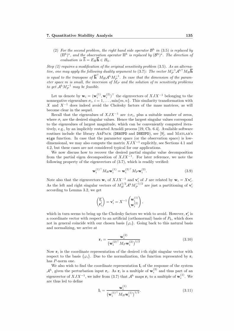
(2) For the second problem, the right hand side operator Bh in (3.5) is replaced by(Πh)⋆, and the observation operator Πh is replaced by (Bh)⋆. The direction ofevaluation is h = EHh ∈ Hh.

Step (2) requires a modification of the original sensitivity problem (3.5). As an alterna-tive, one may apply the following duality argument to (3.7): The vector M−1

P Ah⊤MHh

is equal to the transpose of h⊤MHAhM−1

P . In case that the dimension of the param-eter space m is small, the inversion of MP and the solution of m sensitivity problemsto get AhM−1

P may be feasible.

Let us denote by wi = (w(1)i ,w(2)

i )⊤ the eigenvectors of XJX−1 belonging to thenonnegative eigenvalues σi, i = 1, . . . ,minm,n. This similarity transformation withX and X−1 does indeed avoid the Cholesky factors of the mass matrices, as willbecome clear in the sequel.

Recall that the eigenvalues of XJX−1 are ±σi, plus a suitable number of zeros,where σi are the desired singular values. Hence the largest singular values correspondto the eigenvalues of largest magnitude, which can be conveniently computed itera-tively, e.g., by an implicitly restarted Arnoldi process [19, Ch. 6.4]. Available softwareroutines include the library ArPack (DNAUPD and DNEUPD), see [9], and Matlab’seigs function. In case that the parameter space (or the observation space) is low-dimensional, we may also compute the matrix XJX−1 explicitly, see Sections 4.1 and4.2, but these cases are not considered typical for our applications.

We now discuss how to recover the desired partial singular value decompositionfrom the partial eigen decomposition of XJX−1. For later reference, we note thefollowing property of the eigenvectors of (3.7), which is readily verified:

w(1)⊤i MHw(1)

i = w(2)⊤i MPw(2)

i . (3.9)

Note also that the eigenvectors wi of XJX−1 and v′i of J are related by wi = Xv′i.As the left and right singular vectors of M1/2

H AhM−1/2P are just a partitioning of v′i

according to Lemma 3.2, we get(l′ir′i

)= v′i = X−1

(w(1)

i

w(2)i

),

which in turn seems to bring up the Cholesky factors we wish to avoid. However, r′i isa coordinate vector with respect to an artificial (orthonormal) basis of Ph, which doesnot in general coincide with our chosen basis ϕi. Going back to this natural basisand normalizing, we arrive at

ri =w(2)

i(w(2)⊤

i MPw(2)i

)1/2(3.10)

Now ri is the coordinate representation of the desired i-th right singular vector withrespect to the basis ϕi. Due to the normalization, the function represented by ri

has P -norm one.We also wish to find the coordinate representation li of the response of the system

Ah, given the perturbation input ri. As ri is a multiple of w(2)i and thus part of an

eigenvector of XJX−1, we infer from (3.7) that Ah maps ri to a multiple of w(1)i . We

are thus led to define

li =w(1)

i(w(1)⊤

i MHw(1)i

)1/2. (3.11)


Despite the individual normalizations of w(1)i and w(2)

i , li and ri are still related bythe same proportionality constant:

Ahri = σili, (3.12)

as can be easily verified using (3.9). We have thus proved our main result:

Theorem 3.5. Suppose that σi > 0 is an eigenvalue of the matrix XJX−1 witheigenvector wi = (w(1)

i ,w(2)i )⊤. Let ri and li be given by (3.10) and (3.11), respectively

and let ri = EP ri ∈ Ph and li = EH li ∈ Hh be the functions represented by them.Then the following relations are satisfied:

(a) ‖ri‖P = ‖li‖H = 1.(b) The perturbation ri invokes the first order change σili of magnitude σi in the

observed quantity. In terms of coordinate vectors, Ahri = σili.

Based on these considerations, we propose to compute the desired singular valuedecomposition of M1/2

H AhM−1/2P by iteratively approximation the extreme eigenvalues

and corresponding eigenvectors of XJX−1. This avoids the Cholesky factors of themass matrices, as desired. We summarize the proposed procedure in Algorithm 1.

Algorithm 1

Given: discretized spaces Yh, Uh, Zh and Ph, Hh,a discrete critical point (yh, uh, λh) satisfying (3.2)–(3.4) for p0 ∈ Ph,a routine evaluating XJX−1(h,p)⊤ for any given coordinate vector(h,p)⊤, see Remark 3.4

Desired: a user-defined number s of singular values and perturbation directions(right singular vectors) in coordinate representation, which are of great-est first order impact with respect to the observed quantity

1: Call a routine which iteratively computes the 2s eigenvalues λ1 ≥ λ2 ≥ . . . ≥ λs ≥0 ≥ λs+1 ≥ . . . ≥ λ2s of largest absolute value and corresponding eigenvectors wi

of XJX−1.2: Set σi := λi for i = 1, . . . , s.3: Split wi into (w(1)

i ,w(2)i ) of lengths n and m, respectively, for i = 1, . . . , s.

4: Compute vectors ri and li for i = 1, . . . , s according to (3.10) and (3.11).

Remark 3.6. The singular value decomposition of A and Ah relies on the linearityof the map p 7→ (y, u, λ), which maps a perturbation direction p to the directionalderivative of the optimal solution and adjoint state, compare (2.7)–(2.8). For opti-mal control problems with pointwise control constraints a(x) ≤ u(x) ≤ b(x) almosteverywhere on the control domain, the derivative need not be linear with respect tothe direction, see [4, 10]. The presence of strict complementarity, however, restoresthe linearity. The procedure outlined above carries over to this case, with only minormodifications of the operators Kh and Bh on the so-called active sets, compare also [6].

4. Numerical Examples

We consider as an example the optimal control problem

minimize − 14

∫Ω

y(x) dx+γ

2‖u‖2

L2(C)

s.t.

−κ∆y = χC u on Ω

κ∂

∂ny = α (y − y∞) on ∂Ω.

(4.1)


It represents the optimal heating of a room Ω = (−1, 1)2 ⊂ R2 to maximal averagetemperature y, subject to quadratic control costs. Heating is achieved through tworadiators on some part of the domain C ⊂ Ω, and the heating power u serves as adistributed control variable. κ denotes the constant heat diffusivity, while α is theheat transfer coefficient with the environment. The latter has constant temperaturey∞. α is taken to be zero at the walls but greater than zero at the two windows, seeFigure 4.1.

window 1

window 2

radiator 1

radiator 2

−1 −0.8 −0.6 −0.4 −0.2 0 0.2 0.4 0.6 0.8 1−1

−0.8

−0.6

−0.4

−0.2

0

0.2

0.4

0.6

0.8

1FEM Mesh

Figure 4.1. Layout of the domain and an intermediate finite elementmesh with 4225 vertices (degrees of freedom).

In the sequel, we consider the window heat transfer coefficients as perturbationparameters. As its nominal value, we take

α(x) =

0 at the walls1 at the lower (larger) window # 22 at the upper (smaller) window # 1.

We will explore how the optimal temperature y changes under changes of α. Ourexample fits in the framework of Section 2 with

f(y, u) = −14

∫Ω

y(x) dx +γ

2‖u‖2

L2(C)

e(y, u, p)(ϕ) = κ(∇y,∇ϕ)Ω − (u, ϕ)C − (α(y − y∞), ϕ)∂Ω.

Suitable function spaces for the problem are

Y = H1(Ω), U = L2(C), Z = H1(Ω), P = L2(W1)× L2(W2).

f and e are infinitely differentiable w.r.t. (y, u, p). For any given (y, u, p) ∈ Y ×U ×P ,ey(y, u, p) : Y → Z⋆ is onto and even boundedly invertible. Moreover, the problem isstrictly convex and thus has a unique global solution which satisfies the second-ordercondition. The KKT operator is boundedly invertible. As state observation operator,we will use Π(y, u, λ) = y ∈ H = L2(Ω). Compactness of A then follows from com-pactness of the embedding Y → H . Hence the example satisfies the Assumptions 2.3and 2.8. Note that the parameter enters only in the PDE and not in the objective.

The problem is discretized using standard linear continuous finite elements for thestate and adjoint, and discontinuous piecewise constant elements for the control. Inorder to estimate the order of convergence for the singular values, a hierarchy ofuniformly refined triangular meshes is used. An intermediate mesh is shown in Fig-ure 4.1 (right).

Since the problem has a quadratic objective and a linear PDE constraint, its solutionrequires the solution of only one linear system involving K. Here and throughout,


systems involving K were solved using the conjugate gradient method applied to thereduced Hessian operator

Kred =(−e−1

y eu

id

)⋆(Lyy Lyu

Luy Luu

)(−e−1y eu

id

),

see, e.g., [5,7] for details. The state and adjoint partial differential equations are solvedusing a sparse direct solver.

Figure 4.2 shows the nominal solution (yh, uh) in the case

κ = 1, γ = 0.005, y∞ = 0

C = (−0.8, 0.0)× (0.4, 0.8) ∪ (−0.75, 0.75)× (−0.8,−0.6)

W1 = (−0.75, 0)× 1, W2 = (−0.75, 0.75)× −1.This setup describes the goal to heat up the room to a maximal average temperature(taking control costs into account) at an environmental temperature of 0C. Oneclearly sees how heat is lost through the two windows.

−1 −0.8 −0.6 −0.4 −0.2 0 0.2 0.4 0.6 0.8 1−1

−0.8

−0.6

−0.4

−0.2

0

0.2

0.4

0.6

0.8

1Nominal control

80

85

90

95

100

Figure 4.2. Nominal solution: Optimal state (left) and optimal con-trol (right).

In the sequel, we consider three variations of this problem. In every case, theinsulation of the two windows, i.e., the heat transfer coefficient α restricted to thewindow areas, serves as a perturbation parameter. In Problem 1, this parameter isconstant for each window and it is a spatial function in Problems 2 and 3. The optimaltemperature y is the basis of the observation in all cases. In Problems 1 and 3, weobserve the temperature at every point. In Problem 2, we consider only the averagetemperature throughout the room. Hence, these problems cover all cases where atleast one of the parameter or observation spaces P and H is infinite-dimensional andhigh-dimensional after discretization.

All examples are implemented using Matlab’s PDE toolbox. In every case, weuse Matlab’s eigs function with standard tolerances to compute a partial eigendecomposition of the matrix XJX−1. For Problems 1 and 2, we assemble this matrixexplicitly according to (3.7). For Problem 3, we provide matrix-vector products withXJX−1 according to (3.8). Every matrix-vector product comes at the expense of thesolution of two sensitivity problems (3.5), compare Remark 3.4.

4.1. Problem 1: Few Parameters, Large Observation Space. We begin byconsidering perturbations of the heat transfer coefficient on each window, i.e.,

p = (α|W1 , α|W2) ∈ R2.


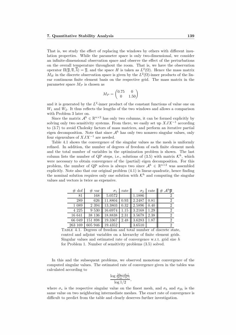
That is, we study the effect of replacing the windows by others with different insu-lation properties. While the parameter space is only two-dimensional, we consideran infinite-dimensional observation space and observe the effect of the perturbationson the overall temperature throughout the room. That is, we have the observationoperator Π(y, u, λ) = y, and the space H is taken as L2(Ω). Hence the mass matrixMH in the discrete observation space is given by the L2(Ω)-inner products of the lin-ear continuous finite element basis on the respective grid. The mass matrix in theparameter space MP is chosen as

MP =(

0.75 00 1.50

)and it is generated by the L2-inner product of the constant functions of value one onW1 and W2. It thus reflects the lengths of the two windows and allows a comparisonwith Problem 3 later on.

Since the matrix Ah ∈ Rn×2 has only two columns, it can be formed explicitly bysolving only two sensitivity systems. From there, we easily set up XJX−1 accordingto (3.7) to avoid Cholesky factors of mass matrices, and perform an iterative partialeigen decomposition. Note that since Ah has only two nonzero singular values, onlyfour eigenvalues of XJX−1 are needed.

Table 4.1 shows the convergence of the singular values as the mesh is uniformlyrefined. In addition, the number of degrees of freedom of each finite element meshand the total number of variables in the optimization problem is shown. The lastcolumn lists the number of QP steps, i.e., solutions of (3.5) with matrix Kh, whichwere necessary to obtain convergence of the (partial) eigen decomposition. For thisproblem, the number of QP solves is always two since Ah ∈ Rn×2 was assembledexplicitly. Note also that our original problem (4.1) is linear-quadratic, hence findingthe nominal solution requires only one solution with Kh and computing the singularvalues and vectors is twice as expensive.

# dof # var σ1 rate σ2 rate # Ahp81 168 5.0572 1.1886 2

289 626 11.8804 0.93 2.2487 0.81 21 089 2 394 13.3803 0.32 2.5896 0.40 24 225 9 530 16.6974 1.15 3.2168 1.29 2

16 641 38 136 18.8838 2.31 3.5678 2.38 266 049 151 898 19.3367 2.48 3.6283 1.87 2

263 169 605 946 19.4352 3.6510 2Table 4.1. Degrees of freedom and total number of discrete state,control and adjoint variables on a hierarchy of finite element grids.Singular values and estimated rate of convergence w.r.t. grid size hfor Problem 1. Number of sensitivity problems (3.5) solved.

In this and the subsequent problems, we observed monotone convergence of thecomputed singular values. The estimated rate of convergence given in the tables wascalculated according to

log |σh−σ∗||σ2h−σ∗|

log 1/2,

where σ∗ is the respective singular value on the finest mesh, and σh and σ2h is thesame value on two neighboring intermediate meshes. The exact rate of convergence isdifficult to predict from the table and clearly deserves further investigation.


On the finest mesh, we obtain as singular values and right singular vectors

σ1 = 19.3367 r1 =(−0.5103−0.7324

)σ2 = 3.6283 r2 =

(−1.03580.3609

).

Recall that r1 and r2 represent piecewise constant functions r1 and r2 on W1 ∪W2

whose values on W1 and W2 are given by the upper and lower entries, respectively,see Figure 4.3 (right). The corresponding left singular vectors are shown in Fig-ure 4.3 (left). These results can be interpreted as follows: Of all perturbations of

−0.8 −0.6 −0.4 −0.2 0 0.2 0.4 0.6 0.8−0.75

−0.7

−0.65

−0.6

−0.55

−0.5Problem 3: First right singular vector (windows 1 and 2)

x position

−0.8 −0.6 −0.4 −0.2 0 0.2 0.4 0.6 0.8−1.2

−1

−0.8

−0.6

−0.4

−0.2

0

0.2

0.4Problem 3: Second right singular vector (windows 1 and 2)

x position

Figure 4.3. Problem 1: First and second left singular vectors l1and l2 (left) and first and second right singular vectors (right), lowerwindow (red) and upper window (blue).

unit size (with respect to the scalar product given by MP ), the nominal state (fromFigure 4.2) is perturbed most (in the L2(Ω)-norm) when both windows are better in-sulated with the ratio of the improvement given by the ratio of the entries of the rightsingular vector r1. The effect of this perturbation direction on the observed quantity(the optimal state) is represented by the first left singular vector l1 = EH l1, multipliedby σ1, compare (3.12). Due to the improved insulation at both windows, l1 is positive,i.e., the optimal temperature increases throughout the domain Ω when p changes fromp0 to p0 + r1. Since the second entry in r1 is greater in magnitude, the effect on theoptimal temperature is more pronounced near the lower window, see Figure 4.3 (topleft).

Since the parameter space is only two-dimensional, the second right singular vec-tor r2 represents the unit perturbation of lowest impact on the optimal state. Fig-ure 4.3 (bottom left) shows the corresponding second left singular vector. Note that


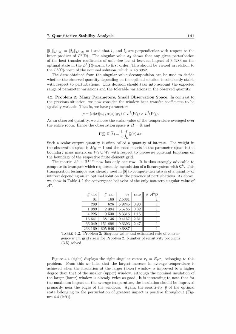
‖l1‖L2(Ω) = ‖l2‖L2(Ω) = 1 and that l1 and l2 are perpendicular with respect to theinner product of L2(Ω). The singular value σ2 shows that any given perturbationof the heat transfer coefficients of unit size has at least an impact of 3.6283 on theoptimal state in the L2(Ω)-norm, to first order. This should be viewed in relation tothe L2(Ω)-norm of the nominal solution, which is 48.3982.

The data obtained from the singular value decomposition can be used to decidewhether the observed quantity depending on the optimal solution is sufficiently stablewith respect to perturbations. This decision should take into account the expectedrange of parameter variations and the tolerable variations in the observed quantity.

4.2. Problem 2: Many Parameters, Small Observation Space. In contrast tothe previous situation, we now consider the window heat transfer coefficients to bespatially variable. That is, we have parameters

p = (α(x)|W1 , α(x)|W2 ) ∈ L2(W1)× L2(W2).

As an observed quantity, we choose the scalar value of the temperature averaged overthe entire room. Hence the observation space is H = R and

Π(y, u, λ) =14

∫Ω

y(x) dx.

Such a scalar output quantity is often called a quantity of interest. The weight inthe observation space is MH = 1 and the mass matrix in the parameter space is theboundary mass matrix on W1 ∪W2 with respect to piecewise constant functions onthe boundary of the respective finite element grid.

The matrix Ah ∈ R1×m now has only one row. It is thus strongly advisable tocompute its transpose which requires only one solution of a linear system withKh. Thistransposition technique was already used in [6] to compute derivatives of a quantity ofinterest depending on an optimal solution in the presence of perturbations. As above,we show in Table 4.2 the convergence behavior of the only non-zero singular value ofAh.

# dof # var σ1 rate # Ahp81 168 2.5381 1

289 626 5.9245 0.93 11 089 2 394 6.6786 0.32 14 225 9 530 8.3316 1.15 1

16 641 38 136 9.4157 2.31 166 049 151 898 9.6393 2.47 1

263 169 605 946 9.6887 1Table 4.2. Problem 2: Singular value and estimated rate of conver-gence w.r.t. grid size h for Problem 2. Number of sensitivity problems(3.5) solved.

Figure 4.4 (right) displays the right singular vector r1 = EP r1 belonging to thisproblem. From this we infer that the largest increase in average temperature isachieved when the insulation at the larger (lower) window is improved to a higherdegree than that of the smaller (upper) window, although the nominal insulation ofthe larger (lower) window is already twice as good. It is interesting to note that forthe maximum impact on the average temperature, the insulation should be improvedprimarily near the edges of the windows. Again, the sensitivity y of the optimalstate belonging to the perturbation of greatest impact is positive throughout (Fig-ure 4.4 (left)).


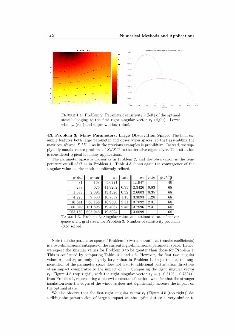
−0.8 −0.6 −0.4 −0.2 0 0.2 0.4 0.6 0.8−0.9

−0.85

−0.8

−0.75

−0.7

−0.65

−0.6

−0.55

−0.5


x position

Figure 4.4. Problem 2: Parametric sensitivity y (left) of the optimalstate belonging to the first right singular vector r1 (right). Lowerwindow (red) and upper window (blue).

4.3. Problem 3: Many Parameters, Large Observation Space. The final ex-ample features both large parameter and observation spaces, so that assembling thematrices Ah and XJX−1 as in the previous examples is prohibitive. Instead, we sup-ply only matrix-vector products of XJX−1 to the iterative eigen solver. This situationis considered typical for many applications.

The parameter space is chosen as in Problem 2, and the observation is the tem-perature on all of Ω as in Problem 1. Table 4.3 shows again the convergence of thesingular values as the mesh is uniformly refined.

# dof # var σ1 rate σ2 rate # Ahp81 168 5.0771 1.1947 40

289 626 11.9262 0.93 2.3426 0.83 681 089 2 394 13.4326 0.32 2.6603 0.35 684 225 9 530 16.7587 1.15 3.3093 1.20 68

16 641 38 136 18.9500 2.31 3.7092 2.31 6866 049 151 898 19.4037 2.48 3.7896 2.31 68

263 169 605 946 19.5024 3.8099 68Table 4.3. Problem 3: Singular values and estimated rate of conver-gence w.r.t. grid size h for Problem 3. Number of sensitivity problems(3.5) solved.

Note that the parameter space of Problem 1 (two constant heat transfer coefficients)is a two-dimensional subspace of the current high-dimensional parameter space. Hence,we expect the singular values for Problem 3 to be greater than those for Problem 1.This is confirmed by comparing Tables 4.1 and 4.3. However, the first two singularvalues σ1 and σ2 are only slightly larger than in Problem 1. In particular, the aug-mentation of the parameter space does not lead to additional perturbation directionsof an impact comparable to the impact of r1. Comparing the right singular vectorr1, Figure 4.5 (top right), with the right singular vector r1 = (−0.5103,−0.7324)⊤

from Problem 1, representing a piecewise constant function, we infer that the strongerinsulation near the edges of the windows does not significantly increase the impact onthe optimal state.

We also observe that the first right singular vector r1 (Figure 4.5 (top right)) de-scribing the perturbation of largest impact on the optimal state is very similar to


−0.8 −0.6 −0.4 −0.2 0 0.2 0.4 0.6 0.8−0.95

−0.9

−0.85

−0.8

−0.75

−0.7

−0.65

−0.6

−0.55

−0.5


x position

−0.8 −0.6 −0.4 −0.2 0 0.2 0.4 0.6 0.8−1.5

−1

−0.5

0

0.5

1

1.5Problem 3: Second right singular vector (windows 1 and 2)

x position

Figure 4.5. Problem 3: First and second left singular vectors (left)and first and second right singular vectors (right), lower window (red)and upper window (blue).

the right singular vector in Problem 2, see Figure 4.4 (right), although the observedquantities are different in Problems 2 and 3.

Finally, we present in Figure 4.6 the distribution of the largest 20 singular values.Their fast decay shows that only a few singular values and the corresponding right sin-gular vectors capture the practically significant perturbation directions of high impactfor the problem at hand.

0 2 4 6 8 10 12 14 16 18 200

2

4

6

8

10

12

14

16

18

20Distribution of the largest singular values

Figure 4.6. Problem 3: First 20 singular values.


5. Conclusion

In this paper, we presented an approach for the quantitative stability analysis oflocal optimal solutions in PDE-constrained optimization. The singular value decom-position of a compact linear operator was used in order to determine the perturbationdirection of greatest impact on an observed quantity which in turn depends on thesolution. After a Galerkin discretization, mass matrices and their Cholesky factorsnaturally appear in the singular value decomposition of the discretized operator. Inorder to avoid forming these Cholesky factors, we described a similarity transformationof the Jordan-Wielandt matrix. A matrix-vector multiplication with this transformedmatrix amounts to the solution of two sensitivity problems. The desired (partial)singular value decomposition can be obtained using standard iterative eigen decom-position software, e.g., implicitly restarted Arnoldi methods.

We presented a number of numerical examples to validate the proposed method andto explain the results in the context of a concrete problem. The order of convergenceof the singular values deserves further investigation. We observed that the numericaleffort even for the computation of few singular values may be large compared to thesolution of the nominal problem itself. In order to accelerate the computation of thedesired singular values and vectors, however, it may be sufficient to compute them ona coarser grid. In addition, parallel implementations of eigen solvers can be used.

References

[1] R. Adams and J. Fournier. Sobolev Spaces. Academic Press, New York, second edition, 2003.[2] K. Deimling. Nonlinear Functional Analysis. Springer, Berlin, 1985.[3] H. Engl, M. Hanke, and A. Neubauer. Regularization of Inverse Problems. Kluwer Academic

Publishers, Boston, 1996.[4] R. Griesse. Parametric sensitivity analysis in optimal control of a reaction-diffusion system—

Part I: Solution differentiability. Numerical Functional Analysis and Optimization, 25(1–2):93–117, 2004.

[5] R. Griesse. Parametric sensitivity analysis in optimal control of a reaction-diffusion system—Part II: Practical methods and examples. Optimization Methods and Software, 19(2):217–242,2004.

[6] R. Griesse and B. Vexler. Numerical sensitivity analysis for the quantity of interest in PDE-constrained optimization. SIAM Journal on Scientific Computing, 29(1):22–48, 2007.

[7] M. Hinze and K. Kunisch. Second order methods for optimal control of time-dependent fluidflow. SIAM Journal on Control and Optimization, 40(3):925–946, 2001.

[8] I. Jolliffe. Principal Component Analysis. Springer, New York, second edition, 2002.[9] R. B. Lehoucq, D. C. Sorensen, and C. Yang. Arpack User’s Guide: Solution of Large-Scale

Eigenvalue Problems with Implicitly Restarted Arnoldi Methods. Software, Environments, andTools. SIAM, Philadelphia, 1998.



infinite-dimensional programming problems. Mathematical Programming, 16:98–110, 1979.[12] J. Nocedal and S. Wright. Numerical Optimization. Springer, New York, 1999.[13] L. Sirovich. Turbulence and the dynamics of coherent structures. I. Quarterly of Applied Math-

ematics, 45(3):561–571, 1987.[14] G. Stewart and J.-G. Sun. Matrix Perturbation Thoery. Academic Press, New York, 1990.[15] F. Troltzsch. On the Lagrange-Newton-SQP method for the optimal control of semilinear para-

bolic equations. SIAM Journal on Control and Optimization, 38(1):294–312, 1999.[16] F. Troltzsch. Optimale Steuerung partieller Differentialgleichungen. Vieweg, Wiesbaden, 2005.[17] F. Troltzsch and D. Wachsmuth. Second-order sufficient optimality conditions for the optimal

control of Navier-Stokes equations. ESAIM: Control, Optimisation and Calculus of Variations,12(1):93–119, 2006.

[18] S. Volkwein. Interpretation of proper orthogonal decomposition as singular value decompositionand HJB-based feedback design. In Proceedings of the Sixteenth International Symposium onMathematical Theory of Networks and Systems (MTNS), Leuven, Belgium, 2004.

[19] D. Watkins. Fundamentals of Matrix Computations. Wiley-Interscience, New York, 2002.


8. Numerical Sensitivity Analysis for the Quantity of Interest 145

8. Numerical Sensitivity Analysis for the Quantity of Interest inPDE-Constrained Optimization

R. Griesse and B. Vexler: Numerical Sensitivity Analysis for the Quantity of Interest inPDE-Constrained Optimization, SIAM Journal on Scientific Computing, 29(1), p.22–48, 2007

As in the previous section, we consider the situation of an observed quantity whichdepends on the solution of an optimization problem subject to perturbations. Thisquantity of interest I, or output functional, is real-valued and and may differ from thecost functional J used during optimization.

Using the notation of the previous section, we introduce the Lagrangian L(y, u, p;π) =J(y, u, π) + 〈p, e(y, u;π)〉 and the reduced cost functional

j(π) = (J Ξ)(π).

We recall that the first-order directional derivatives of j with respect to perturbationssatisfy

(8.1) Dj(π0; δπ) = D(J Ξ)(π0; δπ) = Lπ(Ξ(π0)) δπ.

This is due to the fact that the partial derivatives of Ly, Lu and Lp vanish at Ξ(π0).Moreover, (8.1) continues to hold in the presence of control constraints, see, e.g.Malanowski [2002], or Proposition 3.16 of the paper.

The situation is different for a quantity of interest I 6= J , since the evaluation of itsdirectional derivative D(I Ξ)(π0; δπ) requires the solution of one sensitivity problemto find DΞ(π0; δπ), see Proposition 3.5 and Theorem 3.6 below.

The focus of the present paper is on the efficient evaluation of the gradient and Hessianof the reduced quantity of interest

i(π) = (I Ξ)(π).

It extends results from Becker and Vexler [2005], where the gradient case was in-vestigated. Naturally, the gradient and Hessian information of i and j can be used,for instance, to predict the value of these quantities for perturbed problem settings(compare Section 6).

From the discussion above we conclude that the straightforward evaluation of the gra-dient i′(π0) requires the solution of dim P sensitivity problems (one for each direction),where dim P is the dimension of the parameter space. Using a duality (transposition)argument, we are able to reduce this effort to only one sensitivity problem. With thesame idea, the evaluation of the Hessian can be accomplished by solving 1 + dim Psensitivity problems, rather than O

((dim P )2

)in a straightforward approach. The

duality trick is outlined in Section 3.1 of the paper, and it is elaborated on in Sec-tions 3.2 and 3.3 for problems with and without control constraints. In the controlconstrained case, we need to assume strict complementarity, and, in order for the sec-ond derivative of Ξ(π) to exist, we need to make the additional assumption that theactive sets do not change when moving from the nominal to the perturbed problem,see the text before Theorem 3.19.

The paper concludes with the presentation of an algorithm for the evaluation of thegradient and Hessian of the reduced cost functional and quantity of interest j(π)and i(π), and with two numerical examples which verify the proposed method. Thefirst example is a parameter estimation problem for the incompressible Navier-Stokesequation, and the quantity of interest is either the parameter to be identified, or thedrag of cylinder located in the flow. The scalar perturbation parameter enters oneof the boundary conditions, and no inequality constraints are present. The secondexample is the control constrained boundary optimal control problem for the reaction


diffusion system considered in Section 4 of this thesis. The quantity of interest is thetotal amount of control action over time, and the infinite-dimensional parameter isone of the initial states of the system.

NUMERICAL SENSITIVITY ANALYSIS FOR THE QUANTITY OFINTEREST IN PDE-CONSTRAINED OPTIMIZATION

ROLAND GRIESSE AND BORIS VEXLER

Abstract. In this paper, we consider the efficient computation of derivatives of

a functional (the quantity of interest) which depends on the solution of a PDE-

constrained optimization problem with inequality constraints and which may be

different from the cost functional. The optimization problem is subject to per-

turbations in the data. We derive conditions under with the quantity of inter-

est possesses first and second order derivatives with respect to the perturbation

parameters. An algorithm for the efficient evaluation of these derivatives is de-

veloped, with considerable savings over a direct approach, especially in the case

of high-dimensional parameter spaces. The computational cost is shown to be

small compared to that of the overall optimization algorithm. Numerical exper-

iments involving a parameter identification problem for Navier-Stokes flow and

an optimal control problem for a reaction-diffusion system are presented which

demonstrate the efficiency of the method.

1. Introduction

In this paper we consider PDE-constrained optimization problems with inequalityconstraints. The optimization problems are formulated in a general setting includingoptimal control as well as parameter identification problems. The problems are subjectto perturbation in the data. We suppose to be given a quantity of interest (outputfunctional), which depends on both the state and the control variables and which maybe different from the cost functional used during the optimization.

The quantity of interest is shown to possess first and, under tighter assumptions,second order derivatives with respect to the perturbation parameters. In the presenceof control constraints, strict complementarity and compactness of certain derivativesof the state equation are assumed; for second order derivatives, stability of the activeset is required in addition. The precise conditions are given in Section 3. The maincontribution of this paper is to devise an efficient algorithm to evaluate these sensitivityderivatives, which offers considerable savings over a direct approach, especially inthe case of high-dimensional parameter spaces. We show that the derivatives of thequantity of interest can be computed with only little additional numerical effort incomparison to the corresponding derivatives of the cost functional. Moreover, thecomputational cost for the evaluation of the gradient of the quantity of interest isindependent of the dimension of the parameter space and low compared to that of theoverall optimization algorithm. The cost to evaluate the Hessian grows linearly withthe dimension of the parameter space. We refer to Table 3.1 for details.

The parametric derivatives of the quantity of interest offer a significant amount ofadditional information on top of an optimal solution. The derivative information canbe used to assess the stability of an optimal solution, or to compute a Taylor expansionwhich allows the fast prediction of the perturbed value of the quantity of interest in aneighborhood of a reference parameter.We note that a quantity of interest different from the cost functional is often natural.For instance, an optimization problem in fluid flow may aim at minimizing the dragof a given body, e.g., by adjusting the boundary conditions. The quantity of interest,


however, may be the lift coefficient of the optimal configuration. We also mention theapplicability of our results to bi-level optimization problems where the outer variable isthe ”perturbation” parameter and the outer objective is the output functional, whosederivatives are needed to employ efficient optimization algorithms.

The necessity to compute higher order derivatives may impose possible limitationsto the applicability of the methods presented in this paper. Second order derivativesof the cost functional and the PDE constraint are required to evaluate the gradientof the quantity of interest, and third order derivatives are required to evaluate theHessian.

Let us put our work into perspective. The existence of first and second ordersensitivity derivatives of the objective function (cost functional) in optimal control ofPDEs with control constraints has been proved in [7, 17]. Moreover, [8] addresses thenumerical computation of these derivatives. Recently, the computation of the gradientof the quantity of interest in the absence of inequality constraints has been discussedin [3].

Problem Setting. We consider the PDE-constrained optimization problem in thefollowing abstract form: The state variable u in an appropriate Hilbert space V withscalar product (·, ·)V is determined by a partial differential equation (state equation)in weak form:

a(u, q, p)(φ) = f(φ) ∀φ ∈ V, (1.1)where q denotes the control, or more generally, design variable in the Hilbert spaceQ = L2(ω) with the standard scalar product (·, ·). Typically, ω is a subset of thecomputational domain Ω or a subset of its boundary ∂Ω. In case of finite dimensionalcontrols we set Q = Rn and identify this space with L2(ω) where ω = 1, 2, . . . , n tokeep the notation consistent. The parameter p from a normed linear space P describesthe perturbations of the data.

For fixed p ∈ P, the semi-linear form a(·, ·, p)(·) is defined on the Hilbert spaceV × Q × V. Semi-linear forms are written with two parentheses, the first one refersto the nonlinear arguments, whereas the second one embraces all linear arguments.The partial derivatives of the semi-linear form a(·, ·, p)(·) are denoted by a′u(·, ·, p)(·, ·),a′q(·, ·, p)(·, ·) etc. The linear functional f ∈ V ′ represents the right hand side of thestate equation, where V ′ denotes the dual space of V. For the cost functional (objectivefunctional) we assume the form

J(u, p) +α

2‖q − q‖2Q, (1.2)

which is typical in PDE-constrained optimization problems. Here, α > 0 is a regular-ization parameter and q ∈ Q is a reference control. The functional J : V × P → Ris also subject to perturbation. It is possible to extend our analysis to more generalcost functionals than (1.2). In particular, only notational changes are necessary if Jcontains linear terms in q, and if α and q also depend on the perturbation parame-ter. However, full generality of the cost functional comes at the expense of additionalassumptions which would unnecessarily complicate the discussion.

In order to cover additional control constraints we introduce a nonempty closedconvex subset Qad ⊂ Q by:

Qad = q ∈ Q | b−(x) ≤ q(x) ≤ b+(x) a.e. on ω,with bounds b− ≤ b+ ∈ Q. In the case of finite dimensional controls the inequalityb− ≤ q ≤ b+ is meant to hold componentwise.

The problem under consideration is to

minimize (1.2) over Qad × V (OP(p))

subject to the state equation (1.1)


for fixed p ∈ P. We assume that in a neighbourhood of a reference parameter p0,there exist functions u = U(p) and q = Q(p), which map the perturbation parameterp to a local solution (u, q) of the problem (OP(p)). In Section 3, we give sufficientconditions ensuring the existence and differentiability of these functions. Our resultscomplement previous findings in [7, 10,17].

The quantity of interest is denoted by a functional

I : V ×Q× P → R. (1.3)

This gives rise to the definition of the reduced quantity of interest i : P → R,

i(p) = I(U(p), Q(p), p). (1.4)

Likewise, we denote by j : P → R the reduced cost functional:

j(p) = J(U(p), p) +α

2‖Q(p)− q‖2Q. (1.5)

As stated above, the main contribution of this paper is to devise an efficient algo-rithm to evaluate the first and second derivatives of the reduced quantity of interesti(p).

The outline of the paper is as follows: In the next section we specify the first or-der necessary optimality conditions for the problem under consideration. We recalla primal-dual active set method for its solution. The core step of this method isdescribed to some detail since it is also used for the problems arising during the sensi-tivity computation. In Section 3 we use duality arguments for the efficient evaluationof the first and second order sensitivities of the quantity of interest with respect toperturbation parameters. Throughout, we compare the standard sensitivity analy-sis for the reduced cost functional j(p) with our analysis for the reduced quantity ofinterest i(p). In the last section we discuss two numerical examples illustrating our ap-proach. The first example deals with a parameter identification problem for a channelflow described by the incompressible Navier-Stokes equations. In the second exam-ple we consider the optimal control of time-dependent three-species reaction-diffusionequations under control constraints.

2. Optimization algorithm

In this section we recall the first order necessary conditions for the problem (OP(p))and describe the optimization algorithm with active set strategy which we use in ournumerical examples. In particular, we specify the Newton step taking into account theactive sets since the sensitivity problems arising in Section 3 are solved by the sametechnique.

Throughout the paper we make the following assumption:

Assumption 2.1. (1) Let a(·, ·, ·)(·) be three times continuously differentiable withrespect to (u, q, p).

(2) Let J(·, ·) be three times continuously differentiable with respect to (u, p).(3) Let I(·, ·, ·) be twice continuously differentiable with respect to (u, q, p).

In order to establish the optimality system, we introduce the Lagrangian L : V ×Q× V × P → R as follows:

L(u, q, z, p) = J(u, p) +α

2‖q − q‖2Q + f(z)− a(u, q, p)(z), (2.1)


where z ∈ V denotes the adjoint state. The first order necessary conditions for theproblem (OP(p)) read:

L′u(u, q, z, p)(δu) = 0 ∀δu ∈ V, (2.2)L′q(u, q, z, p)(δq − q) ≥ 0 ∀δq ∈ Qad, (2.3)

L′z(u, q, z, p)(δz) = 0 ∀δz ∈ V. (2.4)

They can be explicitly rewritten as follows:

J ′u(u, p)(δu)− a′u(u, q, p)(δu, z) = 0 ∀δu ∈ V, (2.5)α(q − q, δq − q)− a′q(u, q, p)(δq − q, z) ≥ 0 ∀δq ∈ Qad, (2.6)

f(δz)− a(u, q, p)(δz) = 0 ∀δz ∈ V. (2.7)

For given u, q, z, p, we introduce an additional Lagrange multiplier µ ∈ L2(ω) by thefollowing identification:

(µ, δq) := −L′q(u, q, z, p)(δq)

= −α(q − q, δq) + a′q(u, q, p)(δq, z) ∀δq ∈ L2(ω).

The variational inequality (2.6) is known to be equivalent to the following pointwiseconditions almost everywhere on ω :

q(x) = b−(x) ⇒ µ ≤ 0, (2.8)q(x) = b+(x) ⇒ µ ≥ 0, (2.9)

b−(x) < q(x) < b+(x) ⇒ µ = 0. (2.10)

In addition to the necessary conditions above, in the following lemma we recallsecond order sufficient optimality conditions:

Lemma 2.2 (Sufficient optimality conditions). Let x = (u, q, z) satisfy the first ordernecessary conditions (2.2)–(2.4) of (OP(p)). Moreover, let a′u(u, q, p) : V → V ′ besurjective. If there exists ρ > 0 such that

(δu δq

) [L′′uu(x, p) L′′uq(x, p)L′′qu(x, p) L′′qq(x, p)

](δuδq

)≥ ρ

(‖δu‖2V + ‖δq‖2Q)

holds for all (δu, δq) satisfying the linear (tangent) PDE

a′u(u, q, p)(δu, ϕ) + a′q(u, q, p)(δq, ϕ) = 0 ∀ϕ ∈ V,

then (u, q) is a strict local optimal solution of (OP(p)).

For the proof we refer to [18].For the solution of the first order necessary conditions (2.5)–(2.7) for fixed p ∈ P, we

employ a nonlinear primal-dual active set strategy, see [4, 12, 15, 20]. In the followingwe sketch the corresponding algorithm on the continuous level:


Nonlinear primal-dual active set strategy

(1) Choose initial guess u0, q0, z0, µ0 and c > 0 and set n = 1

(2) While not converged

(3) Determine the active sets An+ and An

−

An− = x ∈ ω | qn−1 + µn−1/c− b− ≤ 0

An+ = x ∈ ω | qn−1 + µn−1/c− b+ ≥ 0

(4) Solve the equality-constrained optimization problem

Minimize J(un, p) +α

2‖qn − q‖2Q over V ×Q

subject to (1.1) and to

qn(x) = b−(x) on An− qn(x) = b+(x) on An

+

with adjoint variable zn

(5) Set µn = −α(qn − q) + a′q(un, qn, p)(·, zn)

(6) Set n = n + 1 and go to 2.

Remark 2.3. (1) The initial guess for the Lagrange multiplier µ0 can be takenaccording to step 5. Another possibility is choosing µ0 = 0 and q0 ∈ Qad, whichleads to solving the optimization problem (step 4) without control constraintsin the first iteration.

(2) The convergence in step 2 can determined conveniently from agreement of theactive sets in two consecutive iterations.

Later on, the above algorithm is applied on the discrete level. The concrete dis-cretization schemes are described in Section 4 for each individual example.

Clearly, the main step in the primal-dual algorithm is the solution of the equality-constrained nonlinear optimization problem in step 4. We shall describe the LagrangeNewton SQP method for its solution in some detail since exactly the same proceduremay be used to solve the sensitivity problems in Section 3, which are the main focusof our paper.

For given active and inactive sets A = A+ ∪ A− and I = ω \ A, let us define the”restriction” operator RI : L2(ω) → L2(ω) by

RI(q) = q · χI ,

where χI is a characteristic function of the set I. Similarly, the operators RA, RA+

and RA− are defined. Note that RI etc. are obviously self-adjoint.


The first order necessary conditions for the purely equality-constrained problem instep 4 are (compare (2.2)–(2.4), respectively (2.5)–(2.7)):

L′u(u, q, z, p)(δu) = 0 ∀δu ∈ V, (2.11)L′q(u, q, z, p)(δq) = 0 ∀δq ∈ L2(In), (2.12)

q − b− = 0 on An− (2.13)

q − b+ = 0 on An+ (2.14)

L′z(u, q, z, p)(δz) = 0 ∀δz ∈ V, (2.15)

with the inactive set In = ω\(An−∪An

+). Using the restriction operators, (2.12)–(2.14)can be reformulated as

L′q(u, q, z, p)(RInδq) + (q − b−, RAn−δq) + (q − b+, RAn

+δq) = 0 ∀δq ∈ Q.

The Lagrange Newton SQP method is defined as Newton’s method, applied to (2.11)–(2.15). To this end, we define B as the Hessian operator of the Lagrangian L, i.e.

B(x, p) =

L′′uu(x, p)(·, ·) L′′uq(x, p)(·, ·) L′′uz(x, p)(·, ·)L′′qu(x, p)(·, ·) L′′qq(x, p)(·, ·) L′′qz(x, p)(·, ·)L′′zu(x, p)(·, ·) L′′zq(x, p)(·, ·) 0

(2.16)

To shorten the notation, we abbreviate x = (u, q, z) and X = V × Q × V. Notethat B(x, p) is a bilinear operator on the space X . By ”multiplication” of B with anelement δx ∈ X from the left, we mean the insertion of the components of δx into thefirst argument. Similarly we define the ”multiplication” of B with an element δx ∈ Xfrom the right as insertion of the components of δx into the second argument. Whenonly one element is inserted, B is interpreted as a linear operator B : X → X ′. In thesequel, we shall omit the (·, ·) notation if no ambiguity arises.In the absence of control constraints, the Newton update (∆u, ∆q, ∆z) for (2.11)–(2.15) at the current iterate (uk, qk, zk) is given by the solution of

B(xk, p)

∆u∆q∆z

= −L′u(xk, p)L′q(xk, p)L′z(xk, p)

. (2.17)

With non-empty active sets An− and An

+, however, (2.17) is replaced by

B(xk, p)

∆u∆q∆z

= − L′u(xk, p)

RInL′q(xk, p) + RAn−(qk − b−) + RAn

+(qk − b+)

L′z(xk, p)

(2.18)

where

B(xk, p) =

idRIn

id

B(xk, p)

idRIn

id

+

0RAn

0

. (2.19)

In other words, B is obtained from B by replacing those components in the derivativeswith respect to the control q by the identity which belong to the active set. In ourpractical realization, we reduce the system (2.18) to the control space L2(ω) usingSchur complement techniques, see, e.g., [16]. The reduced system is solved iterativelyusing the conjugate gradient method, where each step requires the evaluation of amatrix–vector product for the reduced Hessian, which in turn requires the solution ofone tangent and one dual problem, see, e.g., [13], or [2] for a detailed description of thisprocedure in the context of space-time finite element discretization of the problem. Infact, the reduced system needs to be solved only on the currently inactive part L2(In)of the control space since on the active sets, the update ∆q satisfies the trivial relationRAn

±(∆q) = RAn±(b± − qk−1).


The Newton step is completed by applying the update (uk+1, qk+1, zk+1) = (uk, qk, zk)+(∆u, ∆q, ∆z).

3. Sensitivity analysis

In this section we analyze the behavior of local optimal solutions for (OP(p)) underperturbations of the parameter p. We derive formulas for the first and second orderderivatives of the reduced quantity of interest and develop an efficient method for theirevaluation.

To set the stage, we outline the main ideas in Section 3.1 by means of a finite-dimensional optimization problem, without partitioning the optimization variablesinto states and controls, and in the absence of control constraints. To facilitate thediscussion of the infinite-dimensional case, we treat the case of no control constraintsin Section 3.2 and turn to problems with these constraints in Section 3.3. Throughout,we compare the standard sensitivity analysis for the reduced cost functional j(p) (1.5)with our analysis for the reduced quantity of interest i(p) (1.4). The main results canbe found in Theorems 3.6 for the unconstrained case and Theorems 3.18 and 3.21 forthe case with control constraints. An algorithm at the end of Section 3 summarizesthe necessary steps to evaluate the various sensitivity quantities.

3.1. Outline of ideas. Let us consider the nonlinear finite-dimensional equality-constrained optimization problem

Minimize J(x, p) s.t. g(x, p) = 0, (3.1)

where x ∈ Rn denotes the optimization variable, p ∈ Rd is the perturbation parameter,and g : Rn × Rd → Rm collects a number of equality constraints. The Lagrangian of(3.1) is L(x, p) = J(x, p) − z>g(x, p), and under standard constraint qualifications, alocal minimizer x0 of (3.1) at the reference parameter p0 has an associated Lagrangemultiplier z0 ∈ Rm such that

L′x(x0, z0, p0) = J ′x(x0, p0)− z>0 g′x(x0, p0) = 0

L′z(x0, z0, p0) = g(x0, p0) = 0(3.2)

holds. If we assume second order sufficient conditions to hold in addition, then theimplicit function theorem yields the local existence of functions X(p) and Z(p) whichsatisfy (3.2) with p instead of p0, and X(p0) = x0 and Z(p0) = z0 hold. Moreover,(3.2) can be differentiated totally with respect to the parameter and we obtain(L′′xx(x0, z0, p0) g′x(x0, p0)>

g′x(x0, p0) 0

)(X ′(p0) δpZ ′(p0) δp

)= −

(L′′xp(x0, z0, p0) δpg′p(x0, p0) δp

). (3.3)

The solution of (3.3) is a directional derivative of X(p) (and Z(p)) at p = p0, and wenote that it is equivalent to the solution of a linear-quadratic optimization problem.Hence the evaluation of the full Jacobian X ′(p0) requires d = dim P solves of (3.3)with different δp. In our context of large-scale problems, iterative solvers need tobe used and the numerical effort to evaluate the full Jacobian scales linearly with thenumber of right hand sides, i.e., with the dimension of the parameter space d = dim P.

We adapt the definition of the reduced cost functional and the reduced quantityof interest to our current setting, j(p) = J(X(p), p) and i(p) = I(X(p), p). Since wewish to compare the effort to compute the first and second order derivatives of both,we begin by recalling the following result:


Lemma 3.1. Under the conditions above, the reduced cost functional is twice differ-entiable and

j′(p0) δp = L′p(x0, z0, p0) δp

δp>j′′(p0) δp = δp>[L′′px(x0, z0, p0)X ′(p0) δp + L′′pz(x0, z0, p0)Z ′(p0) δp

+ L′′pp(x0, z0, p0) δp].

Proof. We have j(p) = L(X(p), Z(p), p) and hence by the chain rulej′(p0) = L′x(x0, z0, p0)X ′(p0)+L′z(x0, z0, p0)Z ′(p0)+L′p(x0, z0, p0), where the first twoterms vanish in view of (3.2). Differentiating again totally with respect to p yields theexpression for the second derivative.

Lemma 3.1 shows that the evaluation of the gradient of j(·) does not require anylinear solves of the sensitivity system (3.3), while the evaluation of the Hessian requiresd = dim P such solves. The corresponding results for the infinite-dimensional casecan be found below in Propositions 3.5 and 3.16 for the unconstrained and controlconstrained cases.

We will show now that the derivatives of the reduced quantity of interest i(·) can beevaluated efficiently, requiring just one additional system solve. This is a significantimprovement over a direct approach, compare Table 3.1.

From a first look at

i′(p0) δp = I ′x(x0, p0)X ′(p0) δp + I ′p(x0, p0) δp

it seems that the evaluation of the gradient i′(p0) requires d = dim P solves of thesystem (3.3). This is referred to as the direct approach in Table 3.1. However, using(3.3), we may rewrite this as

i′(p0) δp =[−(I ′x(x0, p0), 0

)B−1

0

](L′′xp(x0, z0, p0) δpg′p(x0, p0) δp

)+ I ′p(x0, p0) δp,

where B0 is the matrix on the left hand side of (3.3). Realizing that I ′x(x0, p0) has justone row, evaluating the term in square brackets amounts to only one linear systemsolve. We define the dual quantities (v, y) by

B>0

(vy

)= −

(I ′x(x0, p0)

0

)and finally obtain

i′(p0) δp = v>L′′xp(x0, z0, p0) δp + y>L′′zp(x0, z0, p0) δp + I ′p(x0, p0) δp. (3.4)

We refer to this as a dual approach. In our context, B0 is symmetric and hence thecomputation of the dual quantities requires just one solve of (3.3) with a modifiedright hand side, see again Table 3.1.

For the second derivative, we differentiate (3.4) totally with respect to p. Fromthe chain rule we infer that the sensitivities X ′(p0) and Z ′(p0) now come into play.In addition, v and y need to be differentiated with respect to p, but again a dualitytechnique can be used in order to avoid computing these extra terms. Hence the extracomputational cost to evaluate the Hessian of i(·) amounts to d = dim P solves forthe evaluation of the sensitivity matrices X ′(p0) and Z ′(p0), see Table 3.1. Details canbe found in the proofs of Theorems 3.6 for the unconstrained case and Theorems 3.18and 3.21 for the case with control constraints.


3.2. The case of no control constraints. Throughout this and the following sec-tion, we denote by p0 ∈ P a given reference parameter and by x0 = (u0, q0, z0) asolution to the corresponding first order optimality system (2.11)–(2.15). Moreover,we make the following regularity assumption which we require throughout:

Assumption 3.2. Let the derivative a′u(u0, q0, p0) : V → V ′ be both surjective andinjective, so that it possesses a continuous inverse.

In the case of no control constraints, i.e., Qad = Q, the first order necessary condi-tions (2.11)–(2.15) simplify to

L′u(u, q, z, p)(δu) = 0 ∀δu ∈ V, (3.5)L′q(u, q, z, p)(δq) = 0 ∀δq ∈ Q, (3.6)

L′z(u, q, z, p)(δz) = 0 ∀δz ∈ V. (3.7)

The analysis in this subsection is based on the classical implicit function theorem.We denote by B0 = B(x0, p0) the previously defined Hessian operator at the givenreference solution. For the results in this section we require that B0 is boundedlyinvertible. This property follows from the second order sufficient conditions, see forinstance [14]:

Lemma 3.3. Let the second order sufficient conditions set forth in Lemma 2.2 holdat x0 for OP(p0). Then B0 is boundedly invertible.

The following lemma is a direct application of the implicit function theorem (see [5])to the first order optimality system (3.5)–(3.7).

Lemma 3.4. Let B0 be boundedly invertible. Then there exist neighborhoods N (p0) ⊂P of p0 and N (x0) ⊂ X of x0 and a continuously differentiable function (U,Q,Z) :N (p0) → N (x0) with the following properties:

(a) For every p ∈ N (p0), (U(p), Q(p), Z(p)) is the unique solution to the sys-tem (3.5)–(3.7) in the neighborhood N (x0).

(b) (U(p0), Q(p0), Z(p0)) = (u0, q0, z0) holds.(c) The derivative of (U,Q,Z) at p0 in the direction δp ∈ P is given by the unique

solution of

B0

U ′(p0)(δp)Q′(p0)(δp)Z ′(p0)(δp)

= −L′′up(x0, p0)(·, δp)L′′qp(x0, p0)(·, δp)L′′zp(x0, p0)(·, δp)

. (3.8)

In the following proposition we recall the first and second order sensitivity deriva-tives of the cost functional j(p), compare [17].

Proposition 3.5. Let B0 be boundedly invertible. Then the reduced cost functionalj(p) = J(U(p), p) + α

2 ‖Q(p)− q‖2Q is twice continuously differentiable in N (p0). Thefirst order derivative at p0 in the direction δp ∈ P is given by

j′(p0)(δp) = L′p(x0, p0)(δp). (3.9)

For the second order derivative in the directions of δp and δp, we have

j′′(p0)(δp, δp) = L′′up(x0, p0)(U ′(p)(δp), δp) + L′′qp(x0, p0)(Q′(p)(δp), δp)

+L′′zp(x0, p0)(Z ′(p)(δp), δp) + L′′pp(x0, p0)(δp, δp). (3.10)

Proof. Since (U(p), Q(p)) satisfies the state equation, we have

j(p) = L(U(p), Q(p), Z(p), p)


for all p ∈ N (p0). By the chain rule, the derivative of j(p) reads

j′(p0)(δp) = L′u(x0, p0)(U ′(p0)(δp)) + L′q(x0, p0)(Q′(p0)(δp)) + L′z(x0, p0)(Z ′(p0)(δp))

+L′p(x0, p0)(δp).

The three terms in the first line vanish in view of the optimality system (3.5)–(3.7).Differentiating (3.9) again totally with respect to p in the direction of δp yields (3.10),which completes the proof.

The previous proposition allows to evaluate the first order derivative of the reducedcost functional without computing the sensitivity derivatives of the state, control andadjoint variables. That is, the effort to evaluate j′(p0) is negligible compared to theeffort required to solve the optimization problem. In order to obtain second orderderivative j′′(p0), however, the sensitivity derivatives have to be computed accordingto formula (3.8). This corresponds to the solution of one additional linear-quadraticoptimization problem per perturbation direction δp, whose optimality system is givenby (3.8).

We now turn to our main result in the absence of control constraints. In thefollowing theorem, we show that the first and second order derivatives of the quantityof interest can be evaluated at practically the same effort as those of the cost functional.To this end, we use a duality technique (see Section 3.1) and formulate the followingdual problem for the dual variables v ∈ V, r ∈ Q and y ∈ V:

B0

vry

= −I ′u(q0, u0, p0)

I ′q(q0, u0, p0)0

. (3.11)

We remark that this dual problem involves the same operator matrix B0 as the sensi-tivity problem (3.8) since B0 is self-adjoint.

Theorem 3.6. Let B0 be boundedly invertible. Then the reduced quantity of interesti(p) defined in (1.4) is twice continuously differentiable in N (p0). The first orderderivative at p0 in the direction δp ∈ P is given by

i′(p0)(δp) = L′′up(x0, p0)(v, δp) + L′′qp(x0, p0)(r, δp) + L′′zp(x0, p0)(y, δp)

+ I ′p(u0, q0, p0)(δp). (3.12)

For the second order derivative in the directions of δp and δp, we have

i′′(p0)(δp, δp) = 〈v, η〉V×V′ + 〈r, κ〉Q×Q′ + 〈y, σ〉V×V′

+

U ′(p0)(δp)Q′(p0)(δp)

δp

>I ′′uu(q0, u0, p0) I ′′uq(q0, u0, p0) I ′′up(q0, u0, p0)I ′′qu(q0, u0, p0) I ′′qq(q0, u0, p0) I ′′qp(q0, u0, p0)I ′′pu(q0, u0, p0) I ′′pq(q0, u0, p0) I ′′pp(q0, u0, p0)

U ′(p0)(δp)

Q′(p0)(δp)δp

.

(3.13)


Here, (η, κ, σ) ∈ V ′ ×Q′ × V ′ is given byηκσ

=

L′′′upp()(·, δp, δp)L′′′qpp()(·, δp, δp)L′′′zpp()(·, δp, δp)

+

L′′′upu()(·, δp, U ′(p0)(δp)) + L′′′upq()(·, δp,Q′(p0)(δp) + L′′′upz()(·, δp, Z ′(p0)(δp)L′′′qpu()(·, δp, U ′(p0)(δp)) + L′′′qpq()(·, δp,Q′(p0)(δp) + L′′′qpz()(·, δp, Z ′(p0)(δp)

L′′′zpu()(·, δp, U ′(p0)(δp)) + L′′′zpq()(·, δp,Q′(p0)(δp)

+(B′u()(U ′(p0)(δp)) + B′q()(Q

′(p0)(δp)) + B′z()(Z′(p0)(δp)) + B′p()(δp)

)U ′(p0)(δp)Q′(p0)(δp)Z ′(p0)(δp)

.

Remark 3.7. (a) In the definition of (η, κ, σ) we have abbreviated the evaluationat the point (x0, p0) by ().

(b) The bracket 〈·, ·〉V×V′ in (3.13) denotes the duality pairing between V and itsdual space V ′. For instance, the evaluation of 〈v, η〉V×V′ amounts to pluggingin v instead of · in the definition of η. A similar notation is used for thecontrol space Q.

(c) It is tedious but straightforward to check that (3.13) coincides with (3.10) ifthe quantity of interest is chosen equal to the cost functional. In this case, itfollows from (3.11) that the dual quantities v and r vanish and y = z0 holds.

Proof. (of Theorem 3.6) From the definition of the reduced quantity of interest (1.4),we infer that

i′(p0)(δp) = I ′u(u0, q0, p0)(U ′(p0)(δp)) + I ′q(u0, q0, p0)(Q′(p0)(δp)) + I ′p(u0, q0, p0)(δp)(3.14)

holds. In virtue of (3.8) and (3.11), the sum of the first two terms equals

−I ′u(u0, q0, p0)

I ′q(u0, q0, p0)0

>B−10

L′′up(x0, p0)(·, δp)L′′qp(x0, p0)(·, δp)L′′zp(x0, p0)(·, δp)

=

vry

>L′′up(x0, p0)(·, δp)L′′qp(x0, p0)(·, δp)L′′zp(x0, p0)(·, δp)

which implies (3.12). In order to obtain the second derivative, we differentiate (3.14)totally with respect to p in the direction of δp. This yields

i′′(p0)(δp, δp) =U ′(p0)(δp)Q′(p0)(δp)

δp


U ′(p0)(δp)

Q′(p0)(δp)δp

+

I ′u(u0, q0, p0)I ′q(u0, q0, p0)

0

>U ′′(p0)(δp, δp)

Q′′(p0)(δp, δp)Z ′′(p0)(δp, δp)

. (3.15)

From differentiating (3.8) totally with respect to p in the direction of δp, we obtain

B0

U ′′(p0)(δp, δp)Q′′(p0)(δp, δp)Z ′′(p0)(δp, δp)

= −η

κσ

. (3.16)

From here, (3.13) follows.

The main statement of the previous theorem is that the first and second orderderivatives of the reduced quantity of interest can be evaluated at the additional


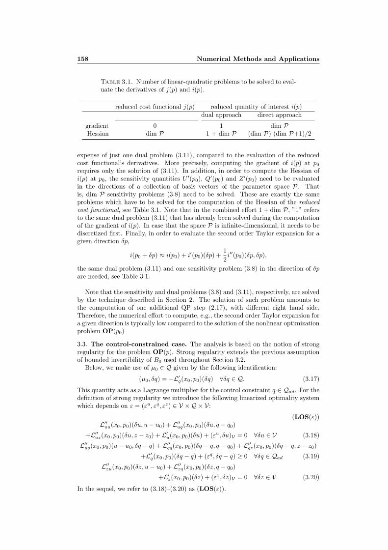
Table 3.1. Number of linear-quadratic problems to be solved to eval-uate the derivatives of j(p) and i(p).

reduced cost functional j(p) reduced quantity of interest i(p)dual approach direct approach

gradient 0 1 dim PHessian dim P 1 + dim P (dim P) (dim P+1)/2

expense of just one dual problem (3.11), compared to the evaluation of the reducedcost functional’s derivatives. More precisely, computing the gradient of i(p) at p0

requires only the solution of (3.11). In addition, in order to compute the Hessian ofi(p) at p0, the sensitivity quantities U ′(p0), Q′(p0) and Z ′(p0) need to be evaluatedin the directions of a collection of basis vectors of the parameter space P. Thatis, dim P sensitivity problems (3.8) need to be solved. These are exactly the sameproblems which have to be solved for the computation of the Hessian of the reducedcost functional, see Table 3.1. Note that in the combined effort 1 + dim P, ”1” refersto the same dual problem (3.11) that has already been solved during the computationof the gradient of i(p). In case that the space P is infinite-dimensional, it needs to bediscretized first. Finally, in order to evaluate the second order Taylor expansion for agiven direction δp,

i(p0 + δp) ≈ i(p0) + i′(p0)(δp) +12i′′(p0)(δp, δp),

the same dual problem (3.11) and one sensitivity problem (3.8) in the direction of δpare needed, see Table 3.1.

Note that the sensitivity and dual problems (3.8) and (3.11), respectively, are solvedby the technique described in Section 2. The solution of such problem amounts tothe computation of one additional QP step (2.17), with different right hand side.Therefore, the numerical effort to compute, e.g., the second order Taylor expansion fora given direction is typically low compared to the solution of the nonlinear optimizationproblem OP(p0)

3.3. The control-constrained case. The analysis is based on the notion of strongregularity for the problem OP(p). Strong regularity extends the previous assumptionof bounded invertibility of B0 used throughout Section 3.2.

Below, we make use of µ0 ∈ Q given by the following identification:

(µ0, δq) = −L′q(x0, p0)(δq) ∀δq ∈ Q. (3.17)

This quantity acts as a Lagrange multiplier for the control constraint q ∈ Qad. For thedefinition of strong regularity we introduce the following linearized optimality systemwhich depends on ε = (εu, εq, εz) ∈ V ×Q× V:

(LOS(ε))L′′uu(x0, p0)(δu, u− u0) + L′′uq(x0, p0)(δu, q − q0)

+L′′uz(x0, p0)(δu, z − z0) + L′u(x0, p0)(δu) + (εu, δu)V = 0 ∀δu ∈ V (3.18)

L′′uq(x0, p0)(u− u0, δq − q) + L′′qq(x0, p0)(δq − q, q − q0) + L′′qz(x0, p0)(δq − q, z − z0)

+L′q(x0, p0)(δq − q) + (εq, δq − q) ≥ 0 ∀δq ∈ Qad (3.19)

L′′zu(x0, p0)(δz, u− u0) + L′′zq(x0, p0)(δz, q − q0)

+L′z(x0, p0)(δz) + (εz, δz)V = 0 ∀δz ∈ V (3.20)

In the sequel, we refer to (3.18)–(3.20) as (LOS(ε)).


Definition 3.8 (Strong Regularity). Let p0 ∈ P be a given reference parameter and letx0 = (u0, q0, z0) be a solution to the corresponding first order optimality system (2.5)–(2.7). If there exist neighborhoods N (0) ⊂ X = V ×Q× V of 0 and N (x0) ⊂ X of x0

such that the following conditions hold:

(a) For every ε ∈ N (0), there exists a solution (uε, qε, zε) to the linearized opti-mality system (3.18)–(3.20).

(b) (uε, qε, zε) is the unique solution of (3.18)–(3.20) in N (x0).(c) (uε, qε, zε) depends Lipschitz-continuously on ε, i.e., there exists L > 0 such

that

‖uε1 − uε2‖V + ‖qε1 − qε2‖Q + ‖zε1 − zε2‖V ≤ L ‖ε1 − ε2‖X (3.21)

holds for all ε1, ε2 ∈ N (0),

then the first order optimality system (2.5)–(2.7) is called strongly regular at x0.

Note that (u0, q0, z0) solves (3.18)–(3.20) for ε = 0. It is not difficult to see that inthe case of no control constraints, i.e., Q = Qad, strong regularity is nothing else thanbounded invertibility of B0 which we had to assume in Section 3.2. In the followinglemma we show that strong regularity holds under suitable second order sufficientoptimality conditions, in analogy to Lemma 3.3. The proof can be carried out usingthe techniques presented in [21].

Lemma 3.9. Let the second order sufficient optimality conditions set forth in Lemma 2.2hold at x0 for OP(p0). Then for any ε ∈ X , (3.18)–(3.20) has a unique solution(uε, qε, zε) and the map

X 3 ε 7→ (uε, qε, zε) ∈ X (3.22)

is Lipschitz continuous. That is, the optimality system is strongly regular at x0.

In the next step, we proceed to prove that the solution (uε, qε, zε) of the linearizedoptimality system (3.18)–(3.20) is directionally differentiable with respect to the per-turbation ε. To this end, we need the following assumption:

Assumption 3.10. At the reference point (u0, q0, z0), let the following linear operatorsbe compact:

(1) V 3 u 7→ a′′qu(u0, q0, p0)(·, u, z0) ∈ Q′

(2) Q 3 q 7→ a′′qq(u0, q0, p0)(·, q, z0) ∈ Q′

(3) V 3 z 7→ a′q(u0, q0, p0)(·, z) ∈ Q′

Remark 3.11. The previous assumption is satisfied for the following important classesof PDE-constrained optimization problems on bounded domains Ω ⊂ Rd, d ∈ 1, 2, 3:

(a) If (OP(p)) is a distributed optimal control problem for a semilinear ellipticPDE, e.g.,

−∆u = f(u) + q on Ω

with V = H10 (Ω) and Q = L2(Ω), then a′′qu = a′′qq = 0 and a′q is the compact

injection of V into Q.(b) In the case of Neumann boundary control on ∂Ω, e.g.,

−∆u = f(u) on Ω and∂

∂nu = q on ∂Ω,

we have V = H1(Ω) and Q = L2(∂Ω). Again, a′′qu = a′′qq = 0 and a′q is thecompact Dirichlet trace operator from V to Q.


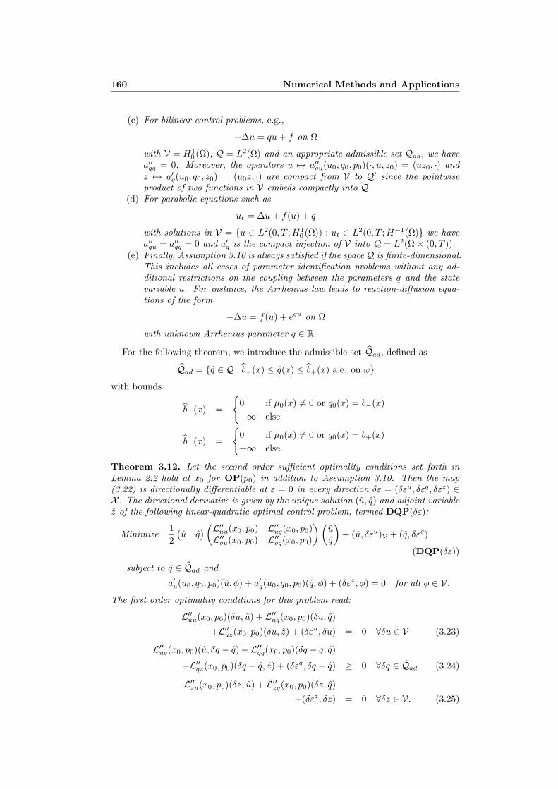
(c) For bilinear control problems, e.g.,

−∆u = qu + f on Ω

with V = H10 (Ω), Q = L2(Ω) and an appropriate admissible set Qad, we have

a′′qq = 0. Moreover, the operators u 7→ a′′qu(u0, q0, p0)(·, u, z0) = (uz0, ·) andz 7→ a′q(u0, q0, z0) = (u0z, ·) are compact from V to Q′ since the pointwiseproduct of two functions in V embeds compactly into Q.

(d) For parabolic equations such as

ut = ∆u + f(u) + q

with solutions in V = u ∈ L2(0, T ;H10 (Ω)) : ut ∈ L2(0, T ;H−1(Ω) we have

a′′qu = a′′qq = 0 and a′q is the compact injection of V into Q = L2(Ω× (0, T )).(e) Finally, Assumption 3.10 is always satisfied if the space Q is finite-dimensional.

This includes all cases of parameter identification problems without any ad-ditional restrictions on the coupling between the parameters q and the statevariable u. For instance, the Arrhenius law leads to reaction-diffusion equa-tions of the form

−∆u = f(u) + equ on Ω

with unknown Arrhenius parameter q ∈ R.

For the following theorem, we introduce the admissible set Qad, defined as

Qad = q ∈ Q : b−(x) ≤ q(x) ≤ b+(x) a.e. on ωwith bounds

b−(x) =

0 if µ0(x) 6= 0 or q0(x) = b−(x)−∞ else

b+(x) =

0 if µ0(x) 6= 0 or q0(x) = b+(x)+∞ else.

Theorem 3.12. Let the second order sufficient optimality conditions set forth inLemma 2.2 hold at x0 for OP(p0) in addition to Assumption 3.10. Then the map(3.22) is directionally differentiable at ε = 0 in every direction δε = (δεu, δεq, δεz) ∈X . The directional derivative is given by the unique solution (u, q) and adjoint variablez of the following linear-quadratic optimal control problem, termed DQP(δε):

Minimize12(u q

)(L′′uu(x0, p0) L′′uq(x0, p0)L′′qu(x0, p0) L′′qq(x0, p0)

)(uq

)+ (u, δεu)V + (q, δεq)

(DQP(δε))

subject to q ∈ Qad and

a′u(u0, q0, p0)(u, φ) + a′q(u0, q0, p0)(q, φ) + (δεz, φ) = 0 for all φ ∈ V.

The first order optimality conditions for this problem read:

L′′uu(x0, p0)(δu, u) + L′′uq(x0, p0)(δu, q)

+L′′uz(x0, p0)(δu, z) + (δεu, δu) = 0 ∀δu ∈ V (3.23)

L′′uq(x0, p0)(u, δq − q) + L′′qq(x0, p0)(δq − q, q)

+L′′qz(x0, p0)(δq − q, z) + (δεq, δq − q) ≥ 0 ∀δq ∈ Qad (3.24)

L′′zu(x0, p0)(δz, u) + L′′zq(x0, p0)(δz, q)

+(δεz, δz) = 0 ∀δz ∈ V. (3.25)


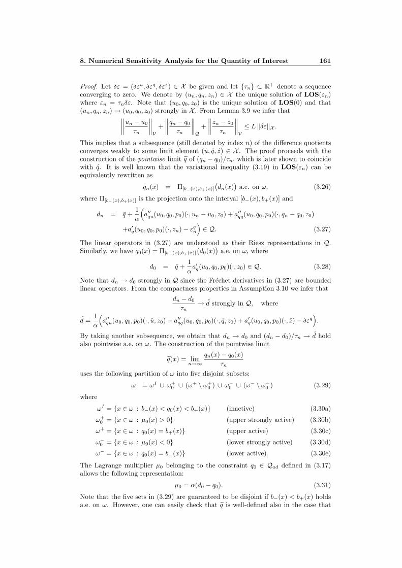
Proof. Let δε = (δεu, δεq, δεz) ∈ X be given and let τn ⊂ R+ denote a sequenceconverging to zero. We denote by (un, qn, zn) ∈ X the unique solution of LOS(εn)where εn = τnδε. Note that (u0, q0, z0) is the unique solution of LOS(0) and that(un, qn, zn) → (u0, q0, z0) strongly in X . From Lemma 3.9 we infer that∥∥∥∥un − u0

τn

∥∥∥∥V

+∥∥∥∥qn − q0

τn

∥∥∥∥Q

+∥∥∥∥zn − z0

τn

∥∥∥∥V≤ L ‖δε‖X .

This implies that a subsequence (still denoted by index n) of the difference quotientsconverges weakly to some limit element (u, q, z) ∈ X . The proof proceeds with theconstruction of the pointwise limit q of (qn − q0)/τn, which is later shown to coincidewith q. It is well known that the variational inequality (3.19) in LOS(εn) can beequivalently rewritten as

qn(x) = Π[b−(x),b+(x)]

(dn(x)

)a.e. on ω, (3.26)

where Π[b−(x),b+(x)] is the projection onto the interval [b−(x), b+(x)] and

dn = q +1α

(a′′qu(u0, q0, p0)(·, un − u0, z0) + a′′qq(u0, q0, p0)(·, qn − q0, z0)

+a′q(u0, q0, p0)(·, zn)− εqn

)∈ Q. (3.27)

The linear operators in (3.27) are understood as their Riesz representations in Q.Similarly, we have q0(x) = Π[b−(x),b+(x)]

(d0(x)

)a.e. on ω, where

d0 = q +1α

a′q(u0, q0, p0)(·, z0) ∈ Q. (3.28)

Note that dn → d0 strongly in Q since the Frechet derivatives in (3.27) are boundedlinear operators. From the compactness properties in Assumption 3.10 we infer that

dn − d0

τn→ d strongly in Q, where

d =1α

(a′′qu(u0, q0, p0)(·, u, z0) + a′′qq(u0, q0, p0)(·, q, z0) + a′q(u0, q0, p0)(·, z)− δεq

).

By taking another subsequence, we obtain that dn → d0 and (dn − d0)/τn → d holdalso pointwise a.e. on ω. The construction of the pointwise limit

q(x) = limn→∞

qn(x)− q0(x)τn

uses the following partition of ω into five disjoint subsets:

ω = ωI ∪ ω+0 ∪ (ω+ \ ω+

0 ) ∪ ω−0 ∪ (ω− \ ω−0 ) (3.29)

where

ωI = x ∈ ω : b−(x) < q0(x) < b+(x) (inactive) (3.30a)

ω+0 = x ∈ ω : µ0(x) > 0 (upper strongly active) (3.30b)

ω+ = x ∈ ω : q0(x) = b+(x) (upper active) (3.30c)

ω−0 = x ∈ ω : µ0(x) < 0 (lower strongly active) (3.30d)

ω− = x ∈ ω : q0(x) = b−(x) (lower active). (3.30e)

The Lagrange multiplier µ0 belonging to the constraint q0 ∈ Qad defined in (3.17)allows the following representation:

µ0 = α(d0 − q0). (3.31)

Note that the five sets in (3.29) are guaranteed to be disjoint if b−(x) < b+(x) holdsa.e. on ω. However, one can easily check that q is well-defined also in the case that


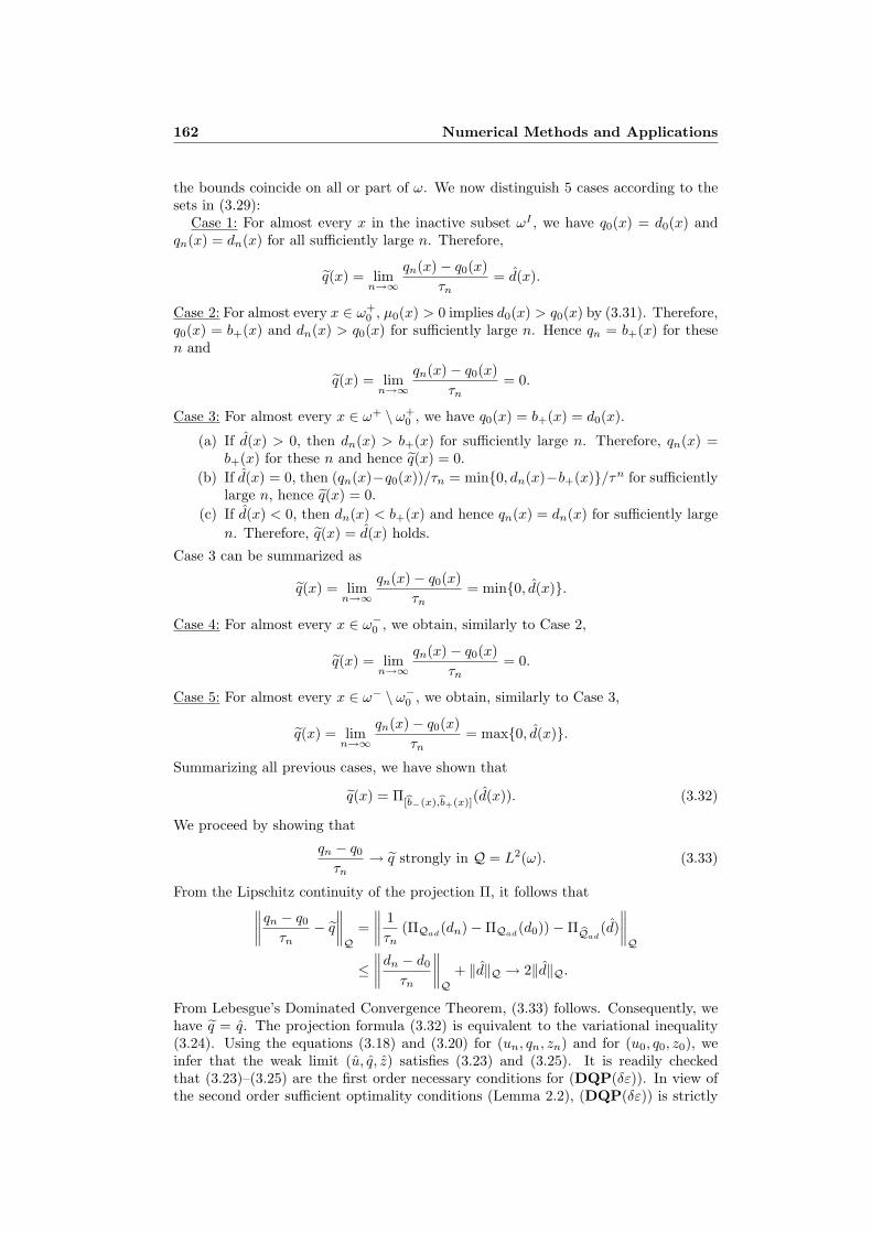
the bounds coincide on all or part of ω. We now distinguish 5 cases according to thesets in (3.29):

Case 1: For almost every x in the inactive subset ωI , we have q0(x) = d0(x) andqn(x) = dn(x) for all sufficiently large n. Therefore,

q(x) = limn→∞

qn(x)− q0(x)τn

= d(x).

Case 2: For almost every x ∈ ω+0 , µ0(x) > 0 implies d0(x) > q0(x) by (3.31). Therefore,

q0(x) = b+(x) and dn(x) > q0(x) for sufficiently large n. Hence qn = b+(x) for thesen and

q(x) = limn→∞

qn(x)− q0(x)τn

= 0.

Case 3: For almost every x ∈ ω+ \ ω+0 , we have q0(x) = b+(x) = d0(x).

(a) If d(x) > 0, then dn(x) > b+(x) for sufficiently large n. Therefore, qn(x) =b+(x) for these n and hence q(x) = 0.

(b) If d(x) = 0, then (qn(x)−q0(x))/τn = min0, dn(x)−b+(x)/τn for sufficientlylarge n, hence q(x) = 0.

(c) If d(x) < 0, then dn(x) < b+(x) and hence qn(x) = dn(x) for sufficiently largen. Therefore, q(x) = d(x) holds.

Case 3 can be summarized as

q(x) = limn→∞

qn(x)− q0(x)τn

= min0, d(x).

Case 4: For almost every x ∈ ω−0 , we obtain, similarly to Case 2,

q(x) = limn→∞

qn(x)− q0(x)τn

= 0.

Case 5: For almost every x ∈ ω− \ ω−0 , we obtain, similarly to Case 3,

q(x) = limn→∞

qn(x)− q0(x)τn

= max0, d(x).

Summarizing all previous cases, we have shown that

q(x) = Π[bb−(x),bb+(x)](d(x)). (3.32)

We proceed by showing that

qn − q0

τn→ q strongly in Q = L2(ω). (3.33)

From the Lipschitz continuity of the projection Π, it follows that∥∥∥∥qn − q0

τn− q

∥∥∥∥Q

=∥∥∥∥ 1

τn(ΠQad

(dn)−ΠQad(d0))−Π bQad

(d)∥∥∥∥Q

≤∥∥∥∥dn − d0

τn

∥∥∥∥Q

+ ‖d‖Q → 2‖d‖Q.

From Lebesgue’s Dominated Convergence Theorem, (3.33) follows. Consequently, wehave q = q. The projection formula (3.32) is equivalent to the variational inequality(3.24). Using the equations (3.18) and (3.20) for (un, qn, zn) and for (u0, q0, z0), weinfer that the weak limit (u, q, z) satisfies (3.23) and (3.25). It is readily checkedthat (3.23)–(3.25) are the first order necessary conditions for (DQP(δε)). In view ofthe second order sufficient optimality conditions (Lemma 2.2), (DQP(δε)) is strictly


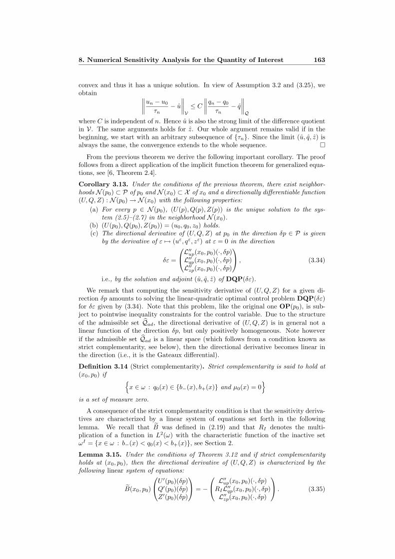
convex and thus it has a unique solution. In view of Assumption 3.2 and (3.25), weobtain ∥∥∥∥un − u0

τn− u

∥∥∥∥V≤ C

∥∥∥∥qn − q0

τn− q

∥∥∥∥Q

where C is independent of n. Hence u is also the strong limit of the difference quotientin V. The same arguments holds for z. Our whole argument remains valid if in thebeginning, we start with an arbitrary subsequence of τn. Since the limit (u, q, z) isalways the same, the convergence extends to the whole sequence.

From the previous theorem we derive the following important corollary. The prooffollows from a direct application of the implicit function theorem for generalized equa-tions, see [6, Theorem 2.4].

Corollary 3.13. Under the conditions of the previous theorem, there exist neighbor-hoods N (p0) ⊂ P of p0 and N (x0) ⊂ X of x0 and a directionally differentiable function(U,Q,Z) : N (p0) → N (x0) with the following properties:

(a) For every p ∈ N (p0), (U(p), Q(p), Z(p)) is the unique solution to the sys-tem (2.5)–(2.7) in the neighborhood N (x0).

(b) (U(p0), Q(p0), Z(p0)) = (u0, q0, z0) holds.(c) The directional derivative of (U,Q,Z) at p0 in the direction δp ∈ P is given

by the derivative of ε 7→ (uε, qε, zε) at ε = 0 in the direction

δε =

L′′up(x0, p0)(·, δp)L′′qp(x0, p0)(·, δp)L′′zp(x0, p0)(·, δp)

, (3.34)

i.e., by the solution and adjoint (u, q, z) of DQP(δε).

We remark that computing the sensitivity derivative of (U,Q,Z) for a given di-rection δp amounts to solving the linear-quadratic optimal control problem DQP(δε)for δε given by (3.34). Note that this problem, like the original one OP(p0), is sub-ject to pointwise inequality constraints for the control variable. Due to the structureof the admissible set Qad, the directional derivative of (U,Q,Z) is in general not alinear function of the direction δp, but only positively homogeneous. Note howeverif the admissible set Qad is a linear space (which follows from a condition known asstrict complementarity, see below), then the directional derivative becomes linear inthe direction (i.e., it is the Gateaux differential).

Definition 3.14 (Strict complementarity). Strict complementarity is said to hold at(x0, p0) if

x ∈ ω : q0(x) ∈ b−(x), b+(x) and µ0(x) = 0

is a set of measure zero.

A consequence of the strict complementarity condition is that the sensitivity deriva-tives are characterized by a linear system of equations set forth in the followinglemma. We recall that B was defined in (2.19) and that RI denotes the multi-plication of a function in L2(ω) with the characteristic function of the inactive setωI = x ∈ ω : b−(x) < q0(x) < b+(x), see Section 2.

Lemma 3.15. Under the conditions of Theorem 3.12 and if strict complementarityholds at (x0, p0), then the directional derivative of (U,Q,Z) is characterized by thefollowing linear system of equations:

B(x0, p0)

U ′(p0)(δp)Q′(p0)(δp)Z ′(p0)(δp)

= − L′′up(x0, p0)(·, δp)

RIL′′qp(x0, p0)(·, δp)L′′zp(x0, p0)(·, δp)

. (3.35)


Moreover, the operator B(x0, p0) : X → X ′ is boundedly invertible.

Proof. In virtue of the strict complementarity property, the admissible set Qad definedin Theorem 3.12 becomes

Qad =

q ∈ Q : q(x) = 0 where q0(x) ∈ b−(x), b+(x)

.

Consequently, the variational inequality (3.24) simplifies to the following equation forQ′(p0)(δp) ∈ Qad:

L′′qu(x0, p0)(δq, U ′(p0)(δp)) + L′′qq(x0, p0)(δq,Q′(p0)(δp))

+ L′′qz(x0, p0)(δq, Z ′(p0)(δp)) = −L′′qp(x0, p0)(δq, δp) ∀δq ∈ Qad,

which is equivalent to the middle equation in (3.35). The first and third equation in(3.35) coincide with (3.23) and (3.25), which proves the first claim. From Theorem 3.12we conclude that B(x0, p0) is bijective. Since it a continuous linear operator fromX → X ′, so is its inverse.

We are now in the position to recall the first and second order sensitivity derivativesof the reduced cost functional j(p), compare again [17]. Note that we do not make useof strict complementarity in the following proposition.

Proposition 3.16. Under the conditions of Theorem 3.12, the reduced cost functional

j(p) = J(U(p), p) +α

2‖Q(p)− q‖2Q

is continuously differentiable in N (p0). The derivative at p0 in the direction δp ∈ Pis given by

j′(p)(δp) = L′p(x0, p0)(δp). (3.36)Additionally, the second order directional derivatives of the reduced cost function jexist, and are given by the following formula:

j′′(p0)(δp, δp) = L′′up(x0, p0)(U ′(p0)(δp), δp) + L′′qp(x0, p0)(Q′(p0)(δp), δp)

+ L′′zp(x0, p0)(Z ′(p0)(δp), δp) + L′′pp(x0, p0)(δp, δp). (3.37)

Proof. As in the unconstrained case there holds:

j′(p0)(δp) = L′u(x0, p0)(U ′(p0)(δp)) + L′q(x0, p0)(Q′(p0)(δp))

+ L′z(x0, p0)(Z ′(p0)(δp)) + L′p(x0, p0)(δp).

and the terms L′u and L′z vanish. Moreover,

L′q(x0, p0)(Q′(p0)(δp)) = −(µ0, Q′(p0)(δp) = 0

since Q′(p0)(δp) is zero on the strongly active set and µ0 vanishes on its complement.The formula for the second order derivative follows as in Proposition 3.5 by totaldirectional differentiation of the first order formula.

Remark 3.17. We note that the expressions for the first and second order derivativesin Proposition 3.16 are the same as in the unconstrained case, see Proposition 3.5.

We now turn to our main result in the control-constrained case, concerning thedifferentiability and efficient evaluation of the sensitivity derivatives for the reducedquantity of interest (1.4). We recall that in the unconstrained case, we have madeuse of a duality argument for the efficient computation of the first and second orderderivatives, see Section 3.2. However, in the presence of control constraints, thistechnique seems to be applicable only in the case of strict complementarity sinceotherwise, the derivatives (U ′(p0)(δp), ξ′(p0)(δp), Z ′(p0)(δp)) do not depend linearly


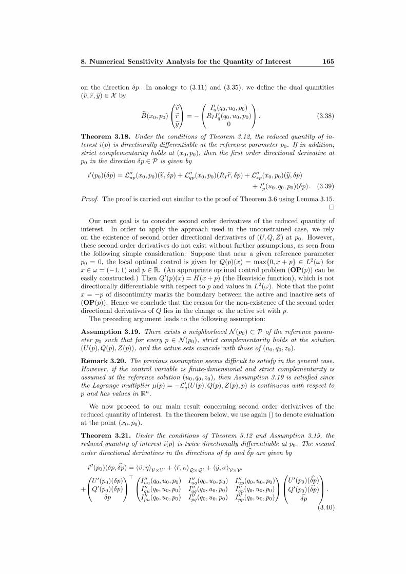
on the direction δp. In analogy to (3.11) and (3.35), we define the dual quantities(v, r, y) ∈ X by

B(x0, p0)

vry

= − I ′u(q0, u0, p0)

RII′q(q0, u0, p0)

0

. (3.38)

Theorem 3.18. Under the conditions of Theorem 3.12, the reduced quantity of in-terest i(p) is directionally differentiable at the reference parameter p0. If in addition,strict complementarity holds at (x0, p0), then the first order directional derivative atp0 in the direction δp ∈ P is given by

i′(p0)(δp) = L′′up(x0, p0)(v, δp) + L′′qp(x0, p0)(RI r, δp) + L′′zp(x0, p0)(y, δp)

+ I ′p(u0, q0, p0)(δp). (3.39)

Proof. The proof is carried out similar to the proof of Theorem 3.6 using Lemma 3.15.

Our next goal is to consider second order derivatives of the reduced quantity ofinterest. In order to apply the approach used in the unconstrained case, we relyon the existence of second order directional derivatives of (U,Q,Z) at p0. However,these second order derivatives do not exist without further assumptions, as seen fromthe following simple consideration: Suppose that near a given reference parameterp0 = 0, the local optimal control is given by Q(p)(x) = max0, x + p ∈ L2(ω) forx ∈ ω = (−1, 1) and p ∈ R. (An appropriate optimal control problem (OP(p)) can beeasily constructed.) Then Q′(p)(x) = H(x + p) (the Heaviside function), which is notdirectionally differentiable with respect to p and values in L2(ω). Note that the pointx = −p of discontinuity marks the boundary between the active and inactive sets of(OP(p)). Hence we conclude that the reason for the non-existence of the second orderdirectional derivatives of Q lies in the change of the active set with p.

The preceding argument leads to the following assumption:

Assumption 3.19. There exists a neighborhood N (p0) ⊂ P of the reference param-eter p0 such that for every p ∈ N (p0), strict complementarity holds at the solution(U(p), Q(p), Z(p)), and the active sets coincide with those of (u0, q0, z0).

Remark 3.20. The previous assumption seems difficult to satisfy in the general case.However, if the control variable is finite-dimensional and strict complementarity isassumed at the reference solution (u0, q0, z0), then Assumption 3.19 is satisfied sincethe Lagrange multiplier µ(p) = −L′q(U(p), Q(p), Z(p), p) is continuous with respect top and has values in Rn.

We now proceed to our main result concerning second order derivatives of thereduced quantity of interest. In the theorem below, we use again () to denote evaluationat the point (x0, p0).

Theorem 3.21. Under the conditions of Theorem 3.12 and Assumption 3.19, thereduced quantity of interest i(p) is twice directionally differentiable at p0. The secondorder directional derivatives in the directions of δp and δp are given by

i′′(p0)(δp, δp) = 〈v, η〉V×V′ + 〈r, κ〉Q×Q′ + 〈y, σ〉V×V′

+

U ′(p0)(δp)Q′(p0)(δp)

δp


U ′(p0)(δp)

Q′(p0)(δp)δp

.

(3.40)


Here, (η, κ, σ) ∈ V ′ ×Q′ × V ′ is given, as in the unconstrained case, by

ηκσ

=

L′′′upp()(·, δp, δp)L′′′qpp()(·, δp, δp)L′′′zpp()(·, δp, δp)

+

L′′′upu()(·, δp, U ′(p0)(δp)) + L′′′upq()(·, δp,Q′(p0)(δp) + L′′′upz()(·, δp, Z ′(p0)(δp)L′′′qpu()(·, δp, U ′(p0)(δp)) + L′′′qpq()(·, δp,Q′(p0)(δp) + L′′′qpz()(·, δp, Z ′(p0)(δp)

L′′′zpu()(·, δp, U ′(p0)(δp)) + L′′′zpq()(·, δp,Q′(p0)(δp)

+(B′u()(U ′(p0)(δp)) + B′q()(Q

′(p0)(δp)) + B′z()(Z′(p0)(δp)) + B′p()(δp)

)U ′(p0)(δp)Q′(p0)(δp)Z ′(p0)(δp)

.

(3.41)

Proof. The proof uses the same argument as the proof of Theorem 3.6. Note that inview of Assumption 3.19, B(U(p), Q(p), Z(p), p) is totally directionally differentiablewith respect to p at p0. In the direction δp, the derivative is

B′u()(U ′(p0)(δp)) + B′q()(Q′(p0)(δp)) + B′z()(Z

′(p0)(δp)) + B′p()(δp).

Due to the constant active sets, these partial derivatives have the following form:

B′u() =

idRI

id

B′u(x0, p0)

idRI

id

,

etc. In view of the bounded invertibility of B(x0, p0), see Lemma 3.15, the secondorder partial derivatives of (U,Q,Z) at p0 exist by the Implicit Function Theorem.They satisfy the analogue of equation (3.16).

We conclude this section by outlining an algorithm which collects the necessary stepsto evaluate the first and second order sensitivity derivatives j′(p0) δp and j′′(p0)(δp, δp)as well as i′(p0) δp and i′′(p0)(δp, δp) for given δp, δp ∈ P. We suppose that the originaloptimization problem (OP(p)) has been solved, e.g., by the primal-dual active setapproach in Section 2, for the nominal parameter p0. We denote by A± and I theactive and inactive sets belonging to the nominal solution (u0, q0) and adjoint statez0. For the definition of B(x0, p0) appearing in equations (3.35) and (3.38), we referto (2.19).


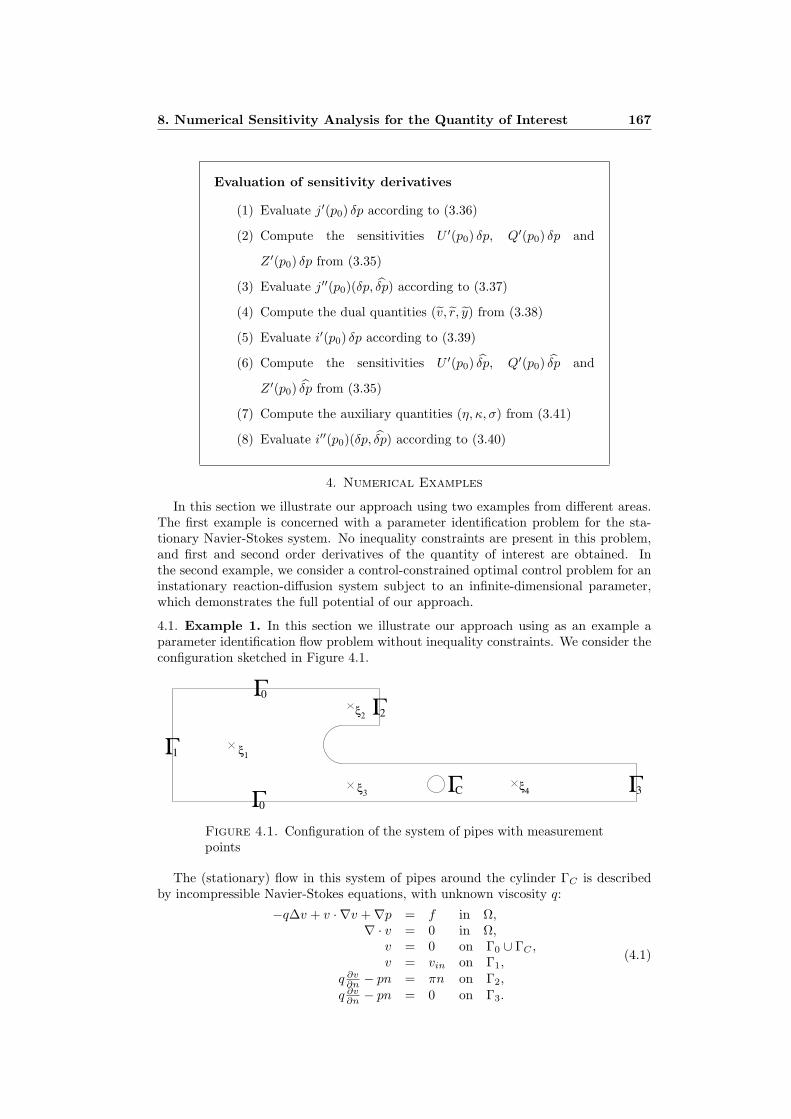
Evaluation of sensitivity derivatives

(1) Evaluate j′(p0) δp according to (3.36)

(2) Compute the sensitivities U ′(p0) δp, Q′(p0) δp and

Z ′(p0) δp from (3.35)

(3) Evaluate j′′(p0)(δp, δp) according to (3.37)

(4) Compute the dual quantities (v, r, y) from (3.38)

(5) Evaluate i′(p0) δp according to (3.39)

(6) Compute the sensitivities U ′(p0) δp, Q′(p0) δp and

Z ′(p0) δp from (3.35)

(7) Compute the auxiliary quantities (η, κ, σ) from (3.41)

(8) Evaluate i′′(p0)(δp, δp) according to (3.40)


In this section we illustrate our approach using two examples from different areas.The first example is concerned with a parameter identification problem for the sta-tionary Navier-Stokes system. No inequality constraints are present in this problem,and first and second order derivatives of the quantity of interest are obtained. Inthe second example, we consider a control-constrained optimal control problem for aninstationary reaction-diffusion system subject to an infinite-dimensional parameter,which demonstrates the full potential of our approach.

4.1. Example 1. In this section we illustrate our approach using as an example aparameter identification flow problem without inequality constraints. We consider theconfiguration sketched in Figure 4.1.

ΓC

Γ1

Γ0

Γ0

Γ2

Γ3

ξ2

ξ

ξ ξ

1

3 4

Figure 4.1. Configuration of the system of pipes with measurementpoints

The (stationary) flow in this system of pipes around the cylinder ΓC is describedby incompressible Navier-Stokes equations, with unknown viscosity q:

−q∆v + v · ∇v +∇p = f in Ω,∇ · v = 0 in Ω,

v = 0 on Γ0 ∪ ΓC ,v = vin on Γ1,

q ∂v∂n − pn = πn on Γ2,

q ∂v∂n − pn = 0 on Γ3.

(4.1)


Here, the state variable u = (v, p) consists of the velocity v = (v1, v2) ∈ H1(Ω)2 andthe pressure p ∈ L2(Ω). The inflow Dirichlet boundary condition on Γ1 is given bya parabolic inflow vin. The outflow boundary conditions of the Neumann type areprescribed on Γ2 and Γ3 involving the perturbation parameter π ∈ P = R. (unlikeprevious sections, we denote the perturbation parameter by π to avoid the confusionwith the pressure p.) Physically, the perturbation parameter π describes the pressuredifference between Γ2 and Γ3, see [11] for detailed discussion of this type of outflowboundary conditions. The reference parameter is chosen π0 = 0.029.

The aim is to estimate the unknown viscosity q ∈ Q = R using the measurementsof the velocity in four given points, see Figure 4.1. By the least squares approach, thisresults in the following parameter identification problem:

Minimize4∑

i=1

2∑j=1

(vj(ξi)− vji )

2 + αq2, subject to (4.1).

Here, vji are the measured values of the components of the velocity at the point ξi

and α is a regularization parameter. For a priori error analysis for finite elementdiscretization of parameter identification problems with pointwise measurements werefer to [19].

The sensitivity analysis of previous sections allows to study the dependence on theperturbation parameter π. To illustrate this, we define two functionals describing thepossible quantities of interest:

I1(u, q) = q, I2(u, q) = cd(u),

where cd(u) is the drag coefficient on the cylinder ΓC defined as:

cd(u) = c0

∫ΓC

n · σ · d ds, (4.2)

with a chosen direction d = (1, 0), given constant c0, and the stress tensor σ given by:

σ =ν

2(∇v + (∇v)T )− pI.

For the discretization of the state equation we use conforming finite elements on ashape-regular quadrilateral mesh Th. The trial and test spaces consist of cell-wise bilin-ear shape-functions for both pressure and velocities. We add further terms to the finiteelement formulation in order to obtain a stable formulation with respect to both thepressure-velocity coupling and convection dominated flow. This type of stabilizationtechniques is based on local projections of the pressure (LPS-method) first introducedin [1]. The resulting parameter identification problem is solved by Newton’s methodon the parameter space as described in [3] which is known to be mesh-independent.The nonlinear state equation is likewise solved by Newton’s method, whereas the lin-ear sub-problems are computed using a standard multi-grid algorithm. With theseingredients, the total numerical cost for the solution of this parameter identificationproblem on a given mesh behaves like O(N), where N is the number of degrees offreedom (dof) for the state equation.

For the reduced quantities of interest i1(π) and i2(π) we compute the first andsecond derivatives using the representations from Theorem 3.6. In Table 4.1 we collectthe values of these derivatives for a sequence of uniformly refined meshes.

In order to verify the computed sensitivity derivatives, we make a comparison withthe derivatives computed by the second order difference quotients. To this end wechoose ε = 10−4 and compute:

dil =il(π0 + ε)− il(π0 − ε)

2 ε, ddil =

il(π0 + ε)− 2il(π0) + il(π0 − ε)ε2

,


Table 4.1. The values of i1(π) and its derivatives on a sequence ofuniformly refined meshes

cells dofs i1(π) i′1(π) i′′1(π)

60 270 1.0176e–2 –3.9712e–1 1.4065e–1240 900 1.0086e–2 –3.9386e–1 –3.2022e–1960 3240 1.0013e–2 –3.9613e–1 –8.5278e–13840 12240 1.0003e–2 –3.9940e–1 –1.0168e–015360 47520 1.0000e–2 –4.0030e–1 –1.0601e–0

Table 4.2. The values of i2(π) and its derivatives on a sequence ofuniformly refined meshes

cells dofs i2(π) i′2(π) i′′2(π)

60 270 3.9511e–1 –13.4846 9.89988240 900 3.9106e–1 –13.8759 –4.09824960 3240 3.9293e–1 –13.8151 16.52393840 12240 3.9242e–1 –13.7357 19.391615360 47520 3.9235e–1 –13.7144 19.9385

by solving the optimization problem additionally for π = π0 − ε and π = π0 + ε. Theresults are shown in Table 4.3.

Remark 4.1. The relative errors in Table 4.3 are of the order of the estimated finitedifference truncation error. We therefore consider the correctness of our method tohave been verified to within the accuracy of this test. The same holds for Example 2and Table 4.4 below.

Table 4.3. Comparison of the computed derivatives of il (l = 1, 2)with difference quotients, on the finest grid

l i′l dildil−i′l

i′li′′l ddil

ddil−i′′li′′l

1 –0.399403 –0.399404 2.5e–6 –1.01676 –1.01678 2.0e–52 –13.73574 –13.73573 –7.3e–7 19.3916 19.3917 5.2e–6

4.2. Example 2. The second example concerns a control-constrained optimal controlproblem for an instationary reaction-diffusion model in 3 spatial dimensions. As theproblem setup was described in detail in [9], we will be brief here. The reaction-diffusion state equation is given by

(c1)t = D1∆c1 − k1c1c2 in Ω× (0, T ), (4.3a)

(c2)t = D2∆c2 − k2c1c2 in Ω× (0, T ), (4.3b)

where ci denotes the concentration of the i-th substance, hence u = (c1, c2) is thestate variable. Ω is a domain in R3, in this case an annular cylinder (Figure 4.2), andT is the given final time. The control q enters through the inhomogeneous boundary


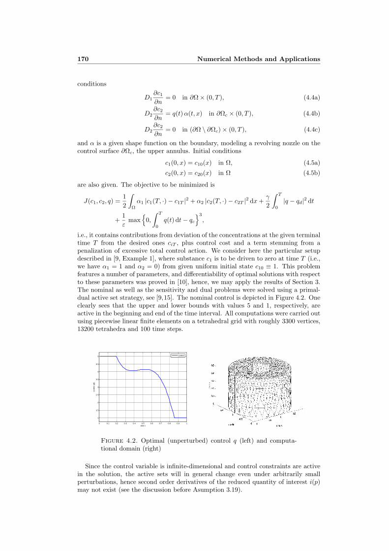
conditions

D1∂c1

∂n= 0 in ∂Ω× (0, T ), (4.4a)

D2∂c2

∂n= q(t) α(t, x) in ∂Ωc × (0, T ), (4.4b)

D2∂c2

∂n= 0 in (∂Ω \ ∂Ωc)× (0, T ), (4.4c)

and α is a given shape function on the boundary, modeling a revolving nozzle on thecontrol surface ∂Ωc, the upper annulus. Initial conditions

c1(0, x) = c10(x) in Ω, (4.5a)

c2(0, x) = c20(x) in Ω (4.5b)

are also given. The objective to be minimized is

J(c1, c2, q) =12

∫Ω

α1 |c1(T, ·)− c1T |2 + α2 |c2(T, ·)− c2T |2 dx +γ

2

∫ T

0

|q − qd|2 dt

+1ε

max

0,

∫ T

0

q(t) dt− qc

3

,

i.e., it contains contributions from deviation of the concentrations at the given terminaltime T from the desired ones ciT , plus control cost and a term stemming from apenalization of excessive total control action. We consider here the particular setupdescribed in [9, Example 1], where substance c1 is to be driven to zero at time T (i.e.,we have α1 = 1 and α2 = 0) from given uniform initial state c10 ≡ 1. This problemfeatures a number of parameters, and differentiability of optimal solutions with respectto these parameters was proved in [10], hence, we may apply the results of Section 3.The nominal as well as the sensitivity and dual problems were solved using a primal-dual active set strategy, see [9,15]. The nominal control is depicted in Figure 4.2. Oneclearly sees that the upper and lower bounds with values 5 and 1, respectively, areactive in the beginning and end of the time interval. All computations were carried outusing piecewise linear finite elements on a tetrahedral grid with roughly 3300 vertices,13200 tetrahedra and 100 time steps.

0 0.1 0.2 0.3 0.4 0.5 0.6 0.7 0.8 0.9 1

1

1.5

2

2.5

3

3.5

4

4.5

5

time t

cont

rol q

(t)

control

Figure 4.2. Optimal (unperturbed) control q (left) and computa-tional domain (right)

Since the control variable is infinite-dimensional and control constraints are activein the solution, the active sets will in general change even under arbitrarily smallperturbations, hence second order derivatives of the reduced quantity of interest i(p)may not exist (see the discussion before Asumption 3.19).


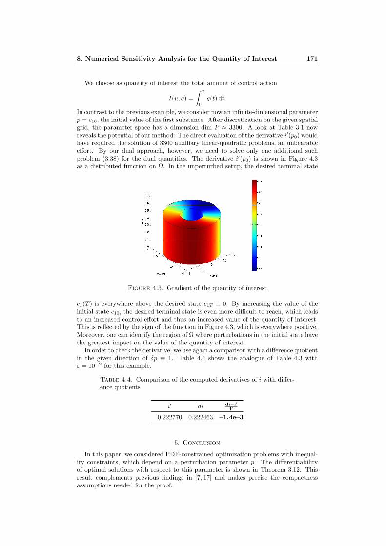
We choose as quantity of interest the total amount of control action

I(u, q) =∫ T

0

q(t) dt.

In contrast to the previous example, we consider now an infinite-dimensional parameterp = c10, the initial value of the first substance. After discretization on the given spatialgrid, the parameter space has a dimension dim P ≈ 3300. A look at Table 3.1 nowreveals the potential of our method: The direct evaluation of the derivative i′(p0) wouldhave required the solution of 3300 auxiliary linear-quadratic problems, an unbearableeffort. By our dual approach, however, we need to solve only one additional suchproblem (3.38) for the dual quantities. The derivative i′(p0) is shown in Figure 4.3as a distributed function on Ω. In the unperturbed setup, the desired terminal state

Figure 4.3. Gradient of the quantity of interest

c1(T ) is everywhere above the desired state c1T ≡ 0. By increasing the value of theinitial state c10, the desired terminal state is even more difficult to reach, which leadsto an increased control effort and thus an increased value of the quantity of interest.This is reflected by the sign of the function in Figure 4.3, which is everywhere positive.Moreover, one can identify the region of Ω where perturbations in the initial state havethe greatest impact on the value of the quantity of interest.

In order to check the derivative, we use again a comparison with a difference quotientin the given direction of δp ≡ 1. Table 4.4 shows the analogue of Table 4.3 withε = 10−2 for this example.

Table 4.4. Comparison of the computed derivatives of i with differ-ence quotients

i′ di di−i′i′

0.222770 0.222463 –1.4e–3

5. Conclusion

In this paper, we considered PDE-constrained optimization problems with inequal-ity constraints, which depend on a perturbation parameter p. The differentiabilityof optimal solutions with respect to this parameter is shown in Theorem 3.12. Thisresult complements previous findings in [7, 17] and makes precise the compactnessassumptions needed for the proof.


We obtained sensitivity results for a quantity of interest which depends on theoptimal solution and is different from the cost functional. The main contribution ofthis paper is to devise an efficient algorithm to evaluate these sensitivity derivatives.Using a duality technique, we showed that the numerical cost of evaluating the gradientor the Hessian of the quantity of interest is only marginally higher than the evaluationof the gradient or the Hessian of the cost functional. The small additional effort is spentfor the solution of one additional linear-quadratic optimization problem for a suitabledual quantity. A comparison with a direct approach for the evaluation of the gradientand the Hessian revealed the tremendous savings of the dual approach especially in thecase of a high-dimenensional parameter space. Two numerical examples confirmed thecorrectness of our derivative formulae and illustrated the applicability of our results.

References

[1] R. Becker and M. Braack. A finite element pressure gradient stabilization for the stokes equations

based on local projections. Calcolo, 38(4):173–199, 2001.

[2] R. Becker, D. Meidner, and B. Vexler. Efficient numerical solution of parabolic optimization

problems by finite element methods. submitted, 2005.

[3] R. Becker and B. Vexler. Mesh refinement and numerical sensitivity analysis for parameter

calibration of partial differential equations. Journal of Computational Physics, 206(1):95–110,

2005.

[4] M. Bergounioux, K. Ito, and K. Kunisch. Primal-dual strategy for constrained optimal control

problems. SIAM Journal on Control and Optimization, 37(4):1176–1194, 1999.

[5] J. Dieudonne. Foundations of Modern Analysis. Academic Press, New York, 1969.

[6] A. Dontchev. Implicit function theorems for generalized equations. Math. Program., 70:91–106,

1995.


Part I: Solution differentiability. Numerical Functional Analysis and Optimization, 25(1–2):93–

117, 2004.


Part II: Practical methods and examples. Optimization Methods and Software, 19(2):217–242,

2004.

[9] R. Griesse and S. Volkwein. A primal-dual active set strategy for optimal boundary control of a

nonlinear reaction-diffusion system. SIAM Journal on Control and Optimization, 44(2):467–494,

2005.

[10] R. Griesse and S. Volkwein. Parametric sensitivity analysis for optimal boundary control of

a 3D reaction-diffusion system. In G. Di Pillo and M. Roma, editors, Large-Scale Nonlinear

Optimization, volume 83 of Nonconvex Optimization and its Applications, pages 127–149, Berlin,

2006. Springer.

[11] J. Heywood, R. Rannacher, and S. Turek. Artificial boundaries and flux and pressure conditions

for the incompressible navier–stokes equations. International Journal for Numerical Methods in

Fluids, 22(5):325–352, 1996.

[12] M. Hintermuller, K. Ito, and K. Kunisch. The primal-dual active set strategy as a semismooth

Newton method. SIAM Journal on Optimization, 13(3):865–888, 2002.

[13] M. Hinze and K. Kunisch. Second Order Methods for Optimal Control of Time-Dependent Fluid

Flow. SIAM Journal on Control and Optimization, 40(3):925–946, 2001.

[14] K. Ito and K. Kunisch. Augmented Lagrangian-SQP Methods in Hilbert Spaces and Application

to Control in the Coefficients Problem. SIAM Journal on Optimization, 6(1):96–125, 1996.

[15] K. Ito and K. Kunisch. The primal-dual active set method for nonlinear optimal control problems

with bilateral constraints. SIAM Journal on Control and Optimization, 43(1):357–376, 2004.

[16] F. Kupfer. An infinite-dimensional convergence theory for reduced SQP methods in Hilbert space.

SIAM Journal on Optimization, 6:126–163, 1996.

[17] K. Malanowski. Sensitivity analysis for parametric optimal control of semilinear parabolic equa-

tions. Journal of Convex Analysis, 9(2):543–561, 2002.


infinite-dimensional programming problems. Mathematical Programming, 16:98–110, 1979.

[19] R. Rannacher and B. Vexler. A priori error estimates for the finite element discretization of elliptic

parameter identification problems with pointwise measurements. SIAM Journal on Control and

Optimization, 44(5):1844–1863, 2005.

[20] A. Rosch and K. Kunisch. A primal-dual active set strategy for a general class of constrained

optimal control problems. SIAM Journal on Optimization, 13(2):321–334, 2002.


[21] F. Troltzsch. Lipschitz stability of solutions of linear-quadratic parabolic control problems with

respect to perturbations. Dynamics of Continuous, Discrete and Impulsive Systems Series A

Mathematical Analysis, 7(2):289–306, 2000.



9. On the Interplay Between Interior Point Approximation andParametric Sensitivities in Optimal Control

R. Griesse and M. Weiser: On the Interplay Between Interior Point Approximation andParametric Sensitivities in Optimal Control, to appear in: Journal of MathematicalAnalysis and Applications, 2007

In all previous publications in this thesis, the primal-dual active set method (seeBergounioux et al. [1999], Hintermuller et al. [2002]) was routinely used in order tocompute optimal solutions and sensitivity derivatives. Interior point methods offer analternative approach to this task. We consider here the classical variant which employsa relaxation (u− ua) η = µ of the complementarity conditions arising in the presenceof, say, a one-sided control constraint u ≥ ua. When the homotopy parameter µ tendsto zero, the corresponding solutions define the so-called central path.

We investigate the interplay between the function space interior point method andparametric sensitivity derivatives for optimization problems of the following kind:

(9.1)Minimize J(u;π) =

12

∫Ω

u(Ku) dx+12

∫Ω

αu2 dx+∫

Ω

f u dx

subject to u− ua ≥ 0 a.e. in Ω.

Here, K is a self-adjoint and positive semidefinite operator in L2(Ω), which mapscompactly into L∞(Ω), f ∈ L∞(Ω), and α ≥ α0 > 0. The perturbation parameterπ may enter K, α and f in a Lipschitz and differentiable way, see Assumption 2.1 ofthe paper. This setting accommodates in particular optimal control problems, whereK = S?S and S is the solution operator of the underlying PDE.

The interior point approach leads to the following relaxed optimality system for (9.1):

(9.2) F (u, η;π, µ) =[Ju(u : π)− η(u− ua) η − µ

]= 0.

The solutions of (9.2) are considered to be functions of both the homotopy parameterµ, viewed as an inner parameter, and the outer parameter π:

Ξ(π, µ) = (Ξu(π, µ),Ξη(π, µ)) = v(π, µ).

Our main results are the following estimates for the convergence of the interior pointapproximations v(π, µ) and their sensitivity derivatives vπ(π, µ) to the exact counter-parts at µ = 0:

‖v(π, µ)− v(π, 0)‖Lq(Ω) ≤ c µ(1+q)/(2q) (Theorem 4.6)

‖vπ(π, µ)− vπ(π, 0)‖Lq(Ω) ≤ cµ1/(2q) (Theorem 4.8)

for all µ < µ0 and q ∈ [2,∞). In other words, the sensitivity derivatives lag behind bya factor of

√µ as µ 0. By excluding a neighborhood of the boundary of the active

set, the convergence rates can be improved by an order of 1/4 (see Theorem 4.9).

These findings are confirmed by three numerical examples in Section 5 of the paper.The first example is a simple problem with K ≡ 0. An elliptic optimal control problemserves as a second example, where the parameter π shifts the desired state. As a thirdexample, we consider an obstacle problem, which fits our setting after switching to itsdual formulation with regularization.

ON THE INTERPLAY BETWEEN INTERIOR POINTAPPROXIMATION AND PARAMETRIC SENSITIVITIES IN

OPTIMAL CONTROL

ROLAND GRIESSE AND MARTIN WEISER

Abstract. Infinite-dimensional parameter-dependent optimization problems ofthe form ’minJ(u; p) subject to g(u) ≥ 0’ are studied, where u is sought in an L∞function space, J is a quadratic objective functional, and g represents pointwiselinear constraints. This setting covers in particular control constrained optimalcontrol problems. Sensitivities with respect to the parameter p of both, optimalsolutions of the original problem, and of its approximation by the classical primal-dual interior point approach are considered. The convergence of the latter to theformer is shown as the homotopy parameter µ goes to zero, and error bounds invarious Lq norms are derived. Several numerical examples illustrate the results.

1. Introduction

In this paper we study infinite-dimensional optimization problems of the form

minuJ(u; p) s.t. g(u) ≥ 0 (1.1)

where u denotes the optimization variable, and p is a parameter in the problem whichis not optimized for. The optimization variable u will be called the control vari-able throughout. It is sought in a suitable function space defined over a domain Ω.The function g(u) represents a pointwise constraint for the control. For simplicity ofthe presentation, we restrict ourselves here to the case of a scalar control, quadraticfunctionals J , and linear constraints. The exact setting is given in Section 2 andaccomodates in particular optimal control of elliptic partial differential equations.

Let us set the dependence of (1.1) on the parameter aside. In the recent past, alot of effort has been devoted to the development of infinite-dimensional algorithmscapable of solving such inequality-constrained problems. Among them are active setstrategies [1, 5–7, 11] and interior point methods [12, 14, 15]. In the latter class, thecomplementarity condition holding for the constraint g(u) ≥ 0 and the correspondingLagrange multiplier η ≥ 0 is relaxed to g(u)η = µ almost everywhere with µ denotingthe duality gap homotopy parameter. When µ is driven to zero, the correspondingrelaxed solutions (u(µ), η(µ)) define the so-called central path.

In a different line of research, the parameter dependence of solutions for optimalcontrol problems with partial differential equations and pointwise control constraintshas been investigated. Differentiability results have been obtained for elliptic [9] andfor parabolic problems [4, 8]. Under certain coercivity assumptions for second orderderivatives, the solutions u(p) were shown to be at least directionally differentiable withrespect to the parameter p. These derivatives, often called parametric sensitivities,allow to assess a solution’s stability properties and to design real-time capable updateschemes.

This paper intends to investigate the interplay between function space interior pointmethods and parametric sensitivity analysis for optimization problems. The solutionsv(p, µ) = (u(p, µ), η(p, µ)) of the interior-point relaxed optimality systems dependon both the homotopy parameter µ, viewed as an inner parameter, and the outer

9. Parametric Sensitivities and Interior Point Methods 175

parameter p. Our main results are, under appropriate assumptions, convergence of theinterior point approximation and its parametric sensitivity to their exact counterparts:

‖v(p, µ)− v(p, 0)‖Lq ≤ c µ(1+q)/(2q) (Theorem 4.6)

‖vp(p, µ)− vp(p, 0)‖Lq ≤ cµ1/(2q) (Theorem 4.8)

for all µ < µ0 and q ∈ [2,∞). By excluding a neighborhood of the boundary ofthe active set, the convergence rates can be improved by an order of 1/4 (Theo-rem 4.9). These convergence rates are confirmed by several numerical examples. Theexamples include a distributed elliptic optimal control problem with pointwise controlconstraints as well as a dualized and regularized obstacle problem.

The outline of the paper is as follows: In Section 2 we define the setting for our prob-lem. Section 3 is devoted to the parametric sensitivity analysis of problem (1.1). InSection 4 we establish our main convergence results, which are confirmed by numericalexamples in Section 5.

Throughout, c denotes a generic positive constant which is independent of thehomotopy parameter µ and the choice of the norm q. It has different values in differentlocations. In case q = ∞, expressions like (r − q)/(2q) are understood in the sense oftheir limit.

By L(X,Y ), we denote the space of linear and continuous operators from X to Y .The (partial) Frechet derivatives of a function G(u, p) are denoted by Gu(u, p) andGp(u, p), respectively. In contrast, we denote the (partial) directional derivative of Gin the direction δp by Dp(G(u, p); δp).

2. Problem Setting

In this section, we define the problem setting and standing assumptions taken tohold throughout the paper. We consider the infinite-dimensional optimization problem

minuJ(u; p) s.t. g(u) ≥ 0. (2.1)

Here, u ∈ L∞(Ω) is the control variable, defined on a bounded domain Ω ⊂ Rd. Forease of notation, we shall denote the standard Lebesgue spaces Lq(Ω) by Lq.

The problem depends on a parameter p from some normed linear space P . Theobjective J : L∞ × P → R is assumed to have the following form:

J(u; p) =12

∫Ω

u(x)((K(p)u)(x)) dx +12

∫Ω

α(x, p)[u(x)]2 dx+∫

Ω

f(x, p)u(x) dx

(2.2)

Assumption 2.1. We assume that p∗ ∈ P is a given reference parameter and thatthe following holds for p in a fixed neighborhood V of p∗:

(a) K(p) : L2 → L∞ is a linear compact operator which is self-adjoint and positivesemidefinite as an operator L2 → L2,

(b) p 7→ K(p) ∈ L(L∞, L∞) is Lipschitz continuous and differentiable,(c) p 7→ α(p) ∈ L∞ is Lipschitz continuous and differentiable,(d) α := infess inf α(p) : p ∈ V > 0,(e) p 7→ f(p) ∈ L∞ is Lipschitz continuous and differentiable.

Note that since∫Ωα(x, p)[u(x)]2 dx ≥ α ‖u‖2L2

, J is strictly convex. In addition, J isweakly lower semicontinuous and radially unbounded and hence (2.1) admits a globalunique minimizer u(p) ∈ L∞ over any nonempty convex closed subset of L∞. Thissetting accomodates in particular optimal control problems with parameter-dependentdesired state yd and objective

J(u; p) =12‖Su− yd(p)‖2L2

+α

2‖u‖2L2


where Su is the unique solution of, e.g., a second-order elliptic partial differentialequation with distributed control u and K = S⋆S. For simplicity of notation, we willfrom now on omit the argument p from K, α and f .

From (2.2) we infer that the objective is differentiable with respect to the norm ofL2 and we identify Ju with its Riesz representative, i.e., we have

Ju(u; p) = Ku+ αu + f.

Note that for u ∈ Lq, Ju(u; p) ∈ Lq holds for all q ∈ [2,∞]. Likewise, we writeJuu(u; p) = K + αI for the second derivative, meaning that

Juu(u; p)(v1, v2) =∫

Ω

v2(Kv1) +∫

Ω

αv1v2.

Let us now turn to the constraints which are given in terms of a Nemyckii operatorinvolving a twice differentiable real function g : R → R with Lipschitz continuousderivatives. For simplicity, we restrict ourselves here to linear control constraints

g(u) = u− a ≥ 0 a.e. on Ω (2.3)

with lower bound a ∈ L∞. The general case is commented on when appropriate. Forlater reference, we define the admissible set

Uad = u ∈ L∞ : g(u) ≥ 0 a.e. on Ω.In this setting, the existence of a regular Lagrange multiplier can be proved:

Lemma 2.2. u is the unique global optimal solution for problem (2.1) if and only ifthere exists a Lagrange multiplier η ∈ L∞ such that the optimality conditions[

Ju(u; p)− gu(u)⋆ηg(u) η

]= 0, g(u) ≥ 0, and η ≥ 0 (2.4)

hold.

Proof. The minimizer u is characterized by the variational inequality

Ju(u; p)(u− u) ≥ 0 for all u ∈ Uad

which can be pointwisely decomposed as Ju(u; p) = 0 where g(u) > 0 and Ju(u; p) ≥ 0where g(u) = 0. Hence, η := Ju(u; p) ∈ L∞ is a multiplier for problem (2.1) suchthat (2.4) is satisfied.

In the general case, the derivative gu(u) extends to a continuous operator from Lq

to Lq (see [14]) and gu(u)⋆ above denotes its L2 adjoint. In view of our choice (2.3)we have gu(u)⋆ = I.

3. Parametric Sensitivity Analysis

In this section we derive a differentiability result for the unrelaxed solution v(p, 0)with respect to changes in the parameter. K, α and f are evaluated at p∗. Moreover,(u∗, η∗) = v(p∗, 0) ∈ L∞ × L∞ is the unique solution of (2.4).

In order to formulate our result, it is useful to define the weakly/strongly activeand inactive subsets for the reference control u∗:

Ω0 = x ∈ Ω : g(u∗) = 0 and η∗ = 0Ω+ = x ∈ Ω : g(u∗) = 0 and η∗ > 0Ωi = x ∈ Ω : g(u∗) > 0 and η∗ = 0

which form a partition of Ω unique up to sets of measure zero. In addition, we define

Uad = u ∈ L∞ : u = 0 a.e. on Ω+ and u ≥ 0 a.e. on Ω0.


Theorem 3.1. Suppose that Assumption 2.1 holds. Then there exist neighborhoodsV ⊂ V of p∗ and U of u∗ and a map

V ∋ p 7→ (u(p), η(p)) ∈ L∞ × L∞

such that u(p) is the unique solution of (2.1) in U and η(p) is the unique Lagrangemultiplier. Moreover, this map is Lipschitz continuous (in the norm of L∞) anddirectionally differentiable at p∗ (in the norm of Lq for all q ∈ [2,∞)). For any givendirection δp, the derivatives δu and δη are the unique solution and Lagrange multiplierin L∞ × L∞ of the auxiliary problem

minδu

12

∫Ω

δu(x)((Kδu)(x)) dx +12

∫Ω

α(x)[δu(x)]2 dx+ Jup(u∗; p∗)(δu, δp)

s.t. δu ∈ Uad. (3.1)

That is, δu and δη satisfy

Kδu+ αδu− δη = −Jup(u∗; p∗)(δu, δp) δu δη = 0 a.e. on Ω,

δu ∈ Uad δη ≥ 0 a.e. on Ω0.(3.2)

Proof. The main tool in deriving the result is the implicit function theorem for gen-eralized equations [3], see Appendix A, which we apply with X = L∞, X = Lq andW = Z = L∞. We formulate (2.4) as a generalized equation. To this end, let

G(u; p) = Ju(u; p)

and

N(u) = ϕ ∈ L∞ :∫

Ω

ϕ (u− u) ≤ 0 for all u ∈ Uad if u ∈ Uad

while N(u) = ∅ otherwise. It is readily seen that (2.4) is equivalent to the generalizedequation

0 ∈ G(u; p) +N(u). (3.3)

Conditions (i) and (ii) of Theorem A.1 are a direct consequence of Assumption 2.1.The verification of conditions (iii) and (iv) proceeds in three steps: constructionof the function ξ, the proof of its Lipschitz continuity, and the proof of directionaldifferentiability.

Step 1: We set up the linearization of (3.3) with respect to u,

δ ∈ G(u∗; p∗) +Gu(u∗; p∗)(u− u∗) +N(u),

which can be written as

δ ∈ Ku+ αu + f +N(u). (3.4)

These are the first order necessary conditions for a perturbation of problem (2.1) withan additional linear term − ∫

Ωδ(x)u(x) dx in the objective, which does not disturb

the strict convexity. Consequently, (3.4) is sufficient for optimality and thus uniquelysolvable for any given δ. This defines the map ξ : L∞ ∋ δ 7→ u = ξ(δ) ∈ L∞ inTheorem A.1.

Step 2: In order to prove that ξ is Lipschitz, let u′ and u′′ be the unique solutionsof (3.4) belonging to δ′ and δ′′. Then (3.4) readily yields∫

Ω

(αu′ +Ku′ + f − δ′)(u′′ − u′) +∫

Ω

(αu′′ +Ku′′ + f − δ′′)(u′ − u′′) ≥ 0.

From there, we obtain

α ‖u′′ − u′‖2L2≤

∫Ω

α (u′′ − u′)2 ≤ ‖δ′′ − δ′‖L2‖u′′ − u′‖L2 −∫

Ω

(u′′ − u′)K(u′′ − u′).


Due to positive semidefiniteness of K,

‖u′′ − u′‖L2 ≤1α‖δ′ − δ′′‖L2 ≤

c

α‖δ′ − δ′′‖L∞

follows. To derive the L∞ estimate, we employ a pointwise argument. Let us denoteby Pu(x) = maxu(x), a(x) the pointwise projection of a function to the admissibleset Uad. As (3.4) is equivalent to

u(x) = P(δ(x) − (Ku)(x)− f(x)

α(x)

),

and the projection is Lipschitz with constant 1, we find that

|u′′(x) − u′(x)| ≤ 1α(x)

(|δ′′(x)− δ′(x)|+ |(K(u′′ − u′))(x)|

)≤ 1α

(‖δ′′ − δ′‖L∞ + ‖K‖L2→L∞‖u′′ − u′‖L2

),

from where the desired ‖u′′ − u′‖L∞ ≤ c ‖δ′ − δ′′‖L∞ follows. Since

‖η′′ − η′‖L∞ = ‖Ju(u′′; p∗)− Ju(u′; p∗)− δ′ + δ′′‖L∞

≤ ‖K(u′′ − u′)‖L∞ + ‖α‖L∞ ‖u′′ − u′‖L∞ + ‖δ′′ − δ′‖L∞

holds, we have Lipschitz continuity also for the Lagrange multiplier.In Step 3 we deduce that u = ξ(δ) in (3.4) depends directionally differentiably on

δ. To this end, let δ ∈ L∞ be a given direction, let τn be a real sequence such thatτn ց 0 and let us define un to be the solution of (3.4) for δn = τnδ. We considerthe difference quotient (un − u∗)/τn which, by the Lipschitz stability shown above, isbounded in L∞ and thus in L2 by a constant times ‖δ‖L∞ . Hence we can extract asubsequence such that

un − u∗

τn u in L2.

By compactness, K((un − u∗)/τn) → Ku in L∞ holds. Hence the sequence dn =−(Kun + f − δn)/α converges uniformly to d∗ = −(Ku∗ + f)/α and (dn − d∗)/τnconverges uniformly to d = (δ − Ku)/α. We now construct a pointwise limit of thedifference quotient taking advantage of the decomposition of Ω. Note that α(u∗−d∗) =η∗ and un = Pdn and likewise u∗ = Pd∗ hold. On Ωi, we have d∗ > a and thus dn > afor sufficiently large n, which entails that

un − u∗

τn=Pdn − Pd∗

τn=dn − d∗

τn→ d on Ωi.

On Ω+, η∗ > 0 implies d∗ < a, hence dn < a for sufficiently large n and thusun − u∗

τn=Pdn − Pd∗

τn=

0− 0τn

→ 0 on Ω+.

Finally on Ω0 we have η∗ = 0 and thus d∗ = a so thatun − u∗

τn=Pdn − Pd∗

τn=Pdn − a

τn→ max

d, 0

on Ω0.

Hence we have constructed a pointwise limit u = lim(un − u∗)/τn on Ω. As∣∣∣∣un − u∗

τn− u

∣∣∣∣ ≤ ∣∣∣∣un − u∗

τn

∣∣∣∣ + |u| ≤∣∣∣∣dn − d∗

τn

∣∣∣∣ + |d|

and the right hand side converges pointwise and in Lq to 2 |d| for any q ∈ [2,∞), weinfer from Lebesgue’s Dominated Convergence Theorem that

un − u∗

τn→ u in Lq for all q ∈ [2,∞)


and hence u = u must hold. As for the Lagrange multiplier, we observe that

ηn − η∗

τn=Ju(un; p∗)− Ju(u∗; p∗)− δn

τn= K

(un − u∗

τn

)+ α

un − u∗

τn− δ

−→ η := Ku+ αu − δ in Lq for all q ∈ [2,∞).

It is straightforward to check that (u, η) are the unique solution and Lagrange multi-plier in L∞ × L∞ of the auxiliary problem

minu

12

∫Ω

u(x)((Ku)(x)) dx +12

∫Ω

α(x)[u(x)]2 dx−∫

Ω

δ(x)u(x) dx s.t. u ∈ Uad.

(3.5)

We are now in the position to apply Theorem A.1 with X = L∞, X = Lq andZ = L∞. It follows that there exists a map V ∋ p 7→ u(p) ∈ U ⊂ L∞ mapping p tothe unique solution of (3.3). Lemma 2.2 shows that u(p) is also the unique solution ofour problem (2.1). Moreover, u(p∗) = u∗ holds, and u(p) is directionally differentiableat p∗ into Lq for any q ∈ [2,∞). By the first equation in (2.4), i.e., η(p) = Ju(u(p); p),the same holds for η(p). The derivative (δu, δη) in the direction of δp is given by theunique solution and Lagrange multiplier of (3.5) with δ = −Jup(u∗; p∗)(·, δp), whosenecessary and sufficient optimality conditions coincide with (3.2). This completes theproof.

Remark 3.2. (1) The directional derivative map

P ∋ δp 7→ (δu, δη) ∈ L∞ × L∞ (3.6)

is positively homogeneous in the direction δp but may be nonlinear. However,‖(δu, δη)‖∞ ≤ c ‖δp‖P holds with c independent of the direction.

(2) In case of Ω0 being a set of measure zero, we say that strict complementarityholds at the solution u(p∗, 0). As a consequence, the admissible set for thesensitivities Uad is a linear space and the map (3.6) is linear.

4. Convergence of Solutions and Parametric Sensitivities

As mentioned in the introduction, we consider an interior point regularization ofproblem (2.1) by means of the classical primal-dual relaxation of the first order neces-sary conditions (2.4). That is, we introduce the homotopy parameter µ ≥ 0 and definethe relaxed optimality system by

F (u, η; p, µ) =[Ju(u; p)− ηg(u) η − µ

]= 0. (4.1)

As opposed to the previous section, we write again p instead of p∗ for the fixed referenceparameter.

Lemma 4.1. For each µ > 0 there exists a unique admissible solution of (4.1).

Proof. A proof is given in [10]. For convenience, we sketch the main ideas here. Theinterior point equation (4.1) is the optimality system for the primal interior pointformulation

min J(u; p)− µ

∫Ω

ln(g(u)) dx

of (1.1). For each ǫ > 0, this functional is lower semicontinuous on the set Mǫ :=u ∈ L∞ : g(u) ≥ ǫ, such that by convexity and coercivity a unique minimizer uǫ(µ)exists. Moreover, if ǫ is sufficiently small, uǫ(µ) = u(µ) ∈ intMǫ holds, such that u(µ)and the associated multiplier satisfy (4.1).


We denote the solution of (4.1) by

v(p, µ) :=(u(p, µ)η(p, µ)

).

It defines the central path homotopy as µց 0 for fixed parameter p.This section is devoted to the convergence analysis of v(p, µ) → v(p, 0) and of

vp(p, µ) → vp(p, 0) as µց 0. We will establish orders of convergence for the full scaleof Lq norms.

In order to avoid cluttered notation with operator norms, we assume throughoutthat δp is an arbitrary parameter direction of unit norm, and we use

vp(p, µ) =(up(p, µ)ηp(p, µ)

)to denote the directional derivative of v(p, µ) in this direction, whose existence isguaranteed by Theorem 3.1 in case µ = 0 and by Lemma 4.7 below for µ > 0.Moreover, we shall omit function arguments when appropriate.

To begin with, we establish the invertibility of the Karush-Kuhn-Tucker operatorbelonging to problem (2.1). Note that gη = µ implies that g + η ≥ 2

√µ.

Lemma 4.2. For any µ > 0, the derivative Fv(v(p, µ); p, µ) is boundedly invertiblefrom Lq → Lq for all q ∈ [2,∞] and satisfies

‖F−1v (·)(a, b)‖Lq ≤ c

(‖a‖Lq +

∥∥∥ b

g + η

∥∥∥Lq

).

Proof. Obviously, F is differentiable with respect to v = (u, η). In view of linearity ofthe inequality constraint, we need to consider the system[

Juu −g⋆u

η gu g

] [uη

]=

[ab

]where the matrix elements are evaluated at u(p, µ) and η(p, µ), respectively. Weintroduce the almost active set ΩA = x ∈ Ω : g ≤ η and its complement ΩI = Ω\ΩA,the almost inactive set. The associated characteristic functions χA and χI = 1− χA,respectively, can be interpreted as orthogonal projectors onto the subspaces L2(ΩA)and L2(ΩI). Dividing the second row by η, we obtain[

Juu −g⋆u

gu (χA + χI) gη

] [u

(χA + χI)η

]=

[a

(χA + χI) bη

].

Eliminating

χI η = χIη

g

(b

η− guu

)and multiplying the second row by −1 leads to the reduced system[

Juu + g⋆uχI

ηg gu −g⋆

u

−gu −χAgη

] [uχAη

]=

[a+ g⋆

uχIbg

−χAbη

].

This linear saddle point problem satisfies the assumptions of Lemma B.1 in [2] (seealso Appendix B) with V = L2(Ω) and M = L2(ΩA): the upper left block is uniformlyelliptic (with constant α independent of µ) and uniformly bounded since η/g ≤ 1 onΩI , the off-diagonal blocks satisfy an inf-sup-condition (independently of µ), and thenegative semidefinite lower right block is uniformly bounded since g/η ≤ 1 on ΩA.Therefore, the operator’s inverse is bounded independently of µ. Using that g ≤ η onΩA and η ≤ g on ΩI , we obtain

‖(u, χAη)‖L2 ≤ c ‖(a+ g⋆uχIb/g, χAb/η)‖L2

≤ c (‖a‖L2 + ‖b/(g + η)‖L2) .


Having the L2-estimate at hand, we can move the spatially coupling operator K tothe right hand side and apply the saddle point lemma pointwisely (with V = M = R)to [

α+ g⋆uχI

ηg gu −g⋆

u

gu χAgη

] [uχAη

]=

[a+ g⋆

uχIbg −Ku

χAbη

].

Since K : L2 → L∞ is compact, we obtain

|(u, χAη)(x)| ≤ c|(a+ g⋆uχIb/g −Ku, χAb/η)|

≤ c (|a|+ |b|/(g + η) + ‖K‖L2→L∞‖u‖L2)

≤ c (|a|+ |b|/(g + η) + ‖a‖L2 + ‖b/(g + η)‖L2)

for almost all x ∈ Ω. From this we conclude that

‖(u, χAη)‖Lq ≤ c(‖a‖Lq + ‖b/(g + η)‖Lq

for all q ≥ 2. Moreover,

‖χI η‖Lq =∥∥∥∥χI

η

g

(b

η− guu

)∥∥∥∥Lq

≤ 2‖b/(g + η)‖Lq + c(‖a‖Lq + ‖b/(g + η)‖Lq)

≤ c(‖a‖Lq + ‖b/(g + η)‖Lq)

holds, which proves the claim.

Remark 4.3. For more complex settings with multicomponent u ∈ Ln∞ and g : Rn →Rm, the proof is essentially the same. The almost active and inactive sets ΩA and ΩI

have to be defined for each component of g separately. The only nontrivial change isto show the inf-sup-condition for gu.

In order to prove convergence of the parametric sensitivities, we will need the strongcomplementarity (cf. [12]) of the non-relaxed solution.

Assumption 4.4. Suppose there exists c > 0 such that the solution v(p, 0) satisfies

|x ∈ Ω : g(u(p, 0)) + η(p, 0) ≤ ǫ| ≤ c ǫr (4.2)

for all ǫ > 0 and some 0 < r ≤ 1.

Note that Assumption 4.4 entails that the set Ω0 of weakly active constraints hasmeasure zero, as

|Ω0| = |⋂ǫ>0

x ∈ Ω : g(u(p, 0)) + η(p, 0) ≤ ǫ| ≤ limǫց0

c ǫr = 0.

In other words, strict complementarity holds at the solution u(p, 0). In our examples,Assumption 4.4 is satisfied with r = 1.

For convenience, we state a special case of Theorem 8.8 from [13] for use in thecurrent setting.

Lemma 4.5. Assume that f ∈ Lq, 1 ≤ q <∞ satisfies∣∣∣x ∈ Ω : |f(x)| > s∣∣∣ ≤ ψ(s), 0 ≤ s <∞,

for some integrable function ψ. Then,

‖f‖qLq≤ q

∫ ∞

0

sq−1ψ(s) ds.

We now prove a bound for the derivative vµ of the central path with respect to theduality gap parameter µ.


Theorem 4.6. Suppose that Assumption 4.4 holds. Then the map µ 7→ v(µ, p) isdifferentiable and the slope of the central path is bounded by

‖vµ(p, µ)‖Lq ≤ c µ(r−q)/(2q), q ∈ [2,∞]. (4.3)

In particular, the a priori error estimate

‖v(p, µ)− v(p, 0)‖Lq ≤ c µ(r+q)/(2q) (4.4)

holds.

Proof. By the implicit function theorem, the derivative vµ is given by

Fv(v(p, µ); p, µ) vµ(p, µ) = −Fµ(v(p, µ); p, µ) =[01

].

Hence from Lemma 4.2 above we obtain

‖vµ(p, µ)‖L∞ ≤ c ‖(g + η)−1‖L∞ ≤ c µ−1/2.

The latter inequality holds since gη = µ implies that g + η ≥ 2√µ.

Now let µn, n ∈ N be a positive sequence converging to zero. We may estimate forn > m

‖v(p, µn)− v(p, µm)‖L∞ ≤∫ µm

µn

‖vµ(p, µ)‖L∞ dµ ≤ c

∫ µm

µn

µ−1/2 dµ

≤ c(µ1/2

m − µ1/2n

)≤ c

√µm,

which is less than any ǫ > 0 for sufficiently large m ≥ mǫ. Thus, v(p, µn) is a Cauchysequence with limit point v. Using continuity of L∞ ∋ v 7→ (Ju(u; p) − η, g(u)η) wefind v = v(p; 0). The limit n→∞ now yields

‖v(p, µ)− v(p, 0)‖L∞ ≤ c√µ, (4.5)

which proves (4.3) and (4.4) for the case q = ∞. From (4.5) and (4.2) we obtain

|x ∈ Ω : g(u(p, µ)) + η(p, µ) < ǫ|

≤

0, if ǫ ≤ 2√µ

|x ∈ Ω : g(u(p, 0)) + η(p, 0) < ǫ+ c√µ| otherwise

≤

0, if ǫ ≤ 2√µ

c (ǫ+ c√µ)r otherwise

with c independent of r. Using Lemmas 4.2 and 4.5 we estimate for q ∈ [2,∞)

‖vµ‖qLq≤ cq ‖(g + η)−1‖q

Lq≤ cqq

∫ ∞

0

sq−1ψ(s) ds

with

ψ(s) =

0, if s ≥ (2

√µ)−1

c (s−1 +√µ)r otherwise


and obtain

‖vµ‖qLq≤ cq+1q

∫ (2√

µ)−1

0

sq−1(s−1 +√µ)r ds

≤ cq+1q

∫ (2√

µ)−1

0

sq−1

(32s−1

)r

ds

= cq+1q(3

2

)r∫ (2

√µ)−1

0

sq−1−r ds

= cq+1 q

q − r

(32

)r [sq−r

](2√µ)−1

0

≤ cq+1 q

q − r3r 2−qµ(r−q)/2.

This implies (4.3). As before in the proof of Theorem 4.6, integration over µ thenyields (4.4).

Lemma 4.7. Along the central path, the solutions v(p, µ) are Frechet differentiablew.r.t. p. There exists µ0 > 0 such that the parametric sensitivities are bounded inde-pendently of µ:

‖vp(p, µ)‖L∞ ≤ c for all µ < µ0.

Proof. By the implicit function theorem and Lemma 4.2, vp exists and satisfies

Fv(v(p, µ); p, µ) vp(p, µ) = −Fp(v(p, µ); p, µ) = −[Jup(u(p, µ); p)

0

]. (4.6)

and ‖vp‖L∞ ≤ c ‖Jup(u(p, µ); p)‖L∞ holds. By (4.4), ‖u(p, µ)‖L∞ is bounded, and byAssumption 2.1, the same holds for ‖Jup(u(p, µ); p)‖L∞ .

Theorem 4.8. Suppose that Assumption 4.4 holds. Then there exist constants µ0 > 0and c independent of µ such that

‖vp(p, µ)− vp(p, 0)‖Lq ≤ cµr/(2q) for all µ < µ0 and q ∈ [2,∞),

where vp(p, 0) is the parametric sensitivity of the original problem.

Proof. We begin with the sensitivity equation (4.6) and differentiate it totally withrespect to µ, which yields

Fvv(vp, vµ) + Fvµvp + Fvvpµ = −Fpvvµ − Fpµ. (4.7)

First we observe Fvµ = 0, Fpµ = 0 and

−Fvv(vp, vµ)− Fpµvµ = −[

Jupuuµ

ηpguuµ + upg⋆uηµ

]=:

[ab

]. (4.8)

In view of Assumption 2.1, Jupu is a fixed element of L(Lq, Lq). Hence by Theorem 4.6,we have

‖a‖Lq ≤ c µ(r−q)/(2q) for all q ∈ [2,∞).

The quantities (uµ, ηµ) and (up, ηp) can be estimated by Theorem 4.6 and Lemma 4.7,respectively, which entails

‖b‖Lq ≤ c(‖ηp‖L∞‖uµ‖Lq + ‖up‖L∞‖ηµ‖Lq

)≤ c µ(r−q)/(2q) for all q ∈ [2,∞)


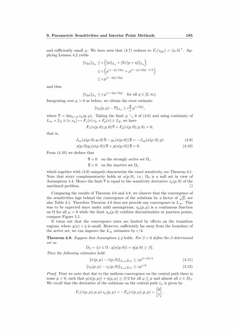
and sufficiently small µ. We have seen that (4.7) reduces to Fv(vpµ) = (a, b)⊤. Ap-plying Lemma 4.2 yields

‖vpµ‖Lq ≤ c(‖a‖Lq + ‖b/(g + η)‖Lq

)≤ c

(µ(r−q)/(2q) + µ(r−q)/(2q)−1/2

)≤ c µ(r−2q)/(2q)

and thus

‖vpµ‖Lq ≤ c µ(r−2q)/(2q) for all q ∈ [2,∞).

Integrating over µ > 0 as before, we obtain the error estimate

‖vp(p, µ)− v‖Lq ≤ cq

rµr/(2q),

where v = limµց0 vp(p, µ). Taking the limit µ ց 0 of (4.6) and using continuity ofL∞ × L2 ∋ (v, vp) 7→ Fv(v) vp + Fp(v) ∈ L2, we have

Fv(v(p, 0); p, 0) v + Fp(v(p, 0); p, 0) = 0,

that is,

Juu(u(p, 0); p, 0)u− gu(u(p; 0)) η = −Jup(u(p, 0); p) (4.9)

η(p, 0)gu(u(p, 0))u+ g(u(p, 0)) η = 0. (4.10)

From (4.10) we deduce that

u = 0 on the strongly active set Ω+

η = 0 on the inactive set Ωi,

which together with (4.9) uniquely characterize the exact sensitivity, see Theorem 3.1.Note that strict complementarity holds at u(p, 0), i.e., Ω0 is a null set in view ofAssumption 4.4. Hence the limit v is equal to the sensitivity derivative vp(p, 0) of theunrelaxed problem.

Comparing the results of Theorem 4.6 and 4.8, we observe that the convergence ofthe sensitivities lags behind the convergence of the solutions by a factor of

√µ, see

also Table 4.1. Therefore Theorem 4.8 does not provide any convergence in L∞. Thiswas to be expected since under mild assumptions, up(p, µ) is a continuous functionon Ω for all µ > 0 while the limit up(p, 0) exhibits discontinuities at junction points,compare Figure 5.1.

It turns out that the convergence rates are limited by effects on the transitionregions, where g(u) + η is small. However, sufficiently far away from the boundary ofthe active set, we can improve the L∞ estimates by r/4:

Theorem 4.9. Suppose that Assumption 4.4 holds. For β > 0 define the β-determinedset as

Dβ = x ∈ Ω : g(u(p, 0)) + η(p, 0) ≥ β.Then the following estimates hold:

‖v(p, µ)− v(p, 0)‖L∞(Dβ) ≤ cµ(r+2)/4 (4.11)

‖vp(p, µ)− vp(p, 0)‖L∞(Dβ) ≤ cµr/4 (4.12)

Proof. First we note that due to the uniform convergence on the central path there issome µ > 0, such that g(u(p, µ)) + η(p, µ) ≥ β/2 for all µ ≤ µ and almost all x ∈ Dβ.We recall that the derivative of the solutions on the central path vµ is given by

Fv(v(p, µ); p, µ) vµ(p, µ) = −Fµ(v(p, µ); p, µ) =[01

].


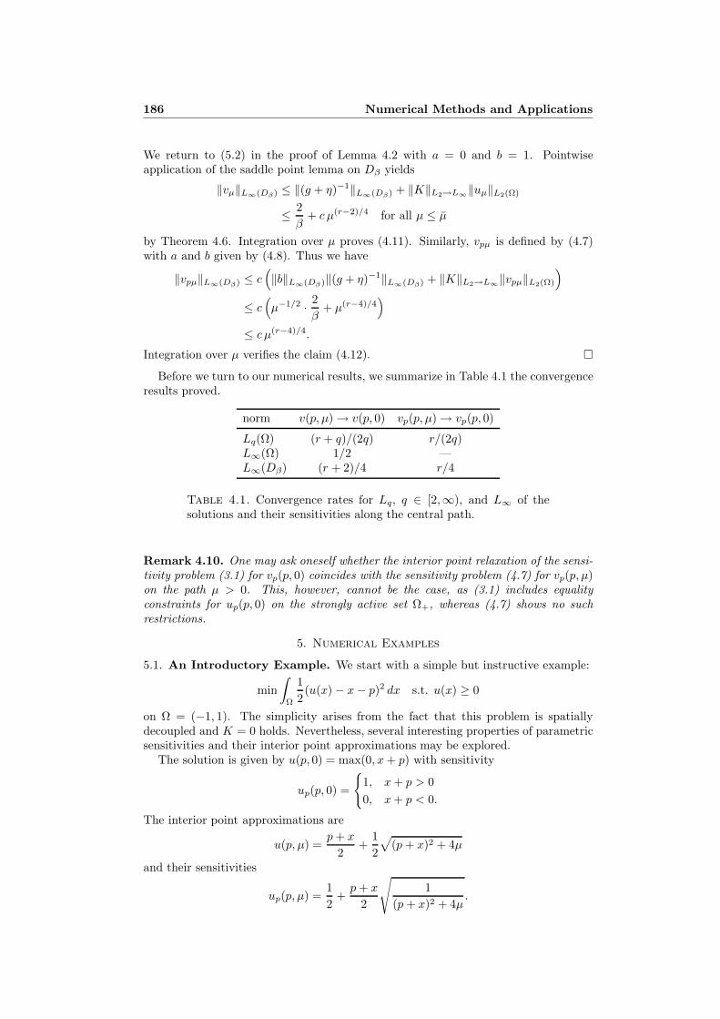
We return to (5.2) in the proof of Lemma 4.2 with a = 0 and b = 1. Pointwiseapplication of the saddle point lemma on Dβ yields

‖vµ‖L∞(Dβ) ≤ ‖(g + η)−1‖L∞(Dβ) + ‖K‖L2→L∞‖uµ‖L2(Ω)

≤ 2β

+ c µ(r−2)/4 for all µ ≤ µ

by Theorem 4.6. Integration over µ proves (4.11). Similarly, vpµ is defined by (4.7)with a and b given by (4.8). Thus we have

‖vpµ‖L∞(Dβ) ≤ c(‖b‖L∞(Dβ)‖(g + η)−1‖L∞(Dβ) + ‖K‖L2→L∞‖vpµ‖L2(Ω)

)≤ c

(µ−1/2 · 2

β+ µ(r−4)/4

)≤ c µ(r−4)/4.

Integration over µ verifies the claim (4.12). Before we turn to our numerical results, we summarize in Table 4.1 the convergence

results proved.

norm v(p, µ) → v(p, 0) vp(p, µ) → vp(p, 0)

Lq(Ω) (r + q)/(2q) r/(2q)L∞(Ω) 1/2 —L∞(Dβ) (r + 2)/4 r/4

Table 4.1. Convergence rates for Lq, q ∈ [2,∞), and L∞ of thesolutions and their sensitivities along the central path.

Remark 4.10. One may ask oneself whether the interior point relaxation of the sensi-tivity problem (3.1) for vp(p, 0) coincides with the sensitivity problem (4.7) for vp(p, µ)on the path µ > 0. This, however, cannot be the case, as (3.1) includes equalityconstraints for up(p, 0) on the strongly active set Ω+, whereas (4.7) shows no suchrestrictions.


5.1. An Introductory Example. We start with a simple but instructive example:

min∫

Ω

12(u(x) − x− p)2 dx s.t. u(x) ≥ 0

on Ω = (−1, 1). The simplicity arises from the fact that this problem is spatiallydecoupled and K = 0 holds. Nevertheless, several interesting properties of parametricsensitivities and their interior point approximations may be explored.

The solution is given by u(p, 0) = max(0, x+ p) with sensitivity

up(p, 0) =

1, x+ p > 00, x+ p < 0.

The interior point approximations are

u(p, µ) =p+ x

2+

12

√(p+ x)2 + 4µ

and their sensitivities

up(p, µ) =12

+p+ x

2

√1

(p+ x)2 + 4µ.


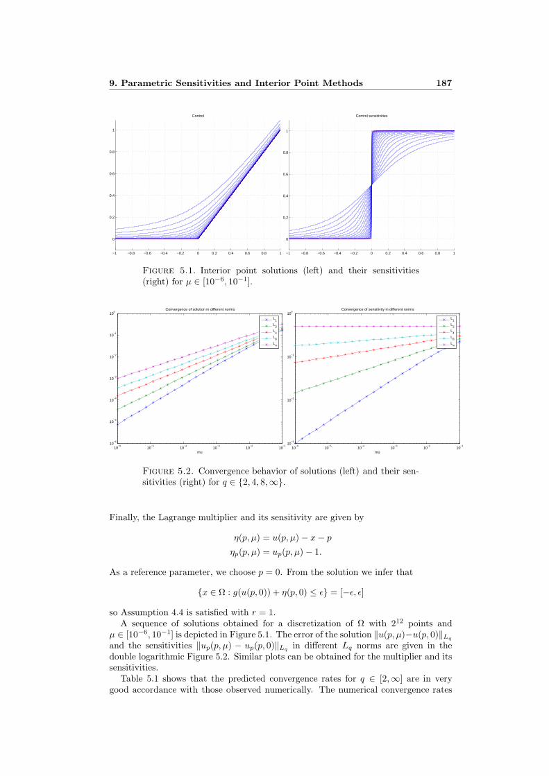
−1 −0.8 −0.6 −0.4 −0.2 0 0.2 0.4 0.6 0.8 1

0

0.2

0.4

0.6

0.8

1

Control

−1 −0.8 −0.6 −0.4 −0.2 0 0.2 0.4 0.6 0.8 1

0

0.2

0.4

0.6

0.8

1

Control sensitivities

Figure 5.1. Interior point solutions (left) and their sensitivities(right) for µ ∈ [10−6, 10−1].

10−6

10−5

10−4

10−3

10−2

10−1

10−6

10−5

10−4

10−3

10−2

10−1

100

Convergence of solution in different norms

mu

L1

L2

L4

L8

L∞

10−6

10−5

10−4

10−3

10−2

10−1

10−3

10−2

10−1

100

Convergence of sensitivity in different norms

mu

L1

L2

L4

L8

L∞

Figure 5.2. Convergence behavior of solutions (left) and their sen-sitivities (right) for q ∈ 2, 4, 8,∞.

Finally, the Lagrange multiplier and its sensitivity are given by

η(p, µ) = u(p, µ)− x− p

ηp(p, µ) = up(p, µ)− 1.

As a reference parameter, we choose p = 0. From the solution we infer that

x ∈ Ω : g(u(p, 0)) + η(p, 0) ≤ ǫ = [−ǫ, ǫ]

so Assumption 4.4 is satisfied with r = 1.A sequence of solutions obtained for a discretization of Ω with 212 points and

µ ∈ [10−6, 10−1] is depicted in Figure 5.1. The error of the solution ‖u(p, µ)−u(p, 0)‖Lq

and the sensitivities ‖up(p, µ) − up(p, 0)‖Lq in different Lq norms are given in thedouble logarithmic Figure 5.2. Similar plots can be obtained for the multiplier and itssensitivities.

Table 5.1 shows that the predicted convergence rates for q ∈ [2,∞] are in verygood accordance with those observed numerically. The numerical convergence rates


control control sensitivityq predicted observed predicted observed

1 — 0.9132 — 0.49602 0.7500 0.7476 0.2500 0.24814 0.6250 0.6221 0.1250 0.12148 0.5625 0.5571 0.0625 0.0565∞ 0.5000 0.5000 — —

Table 5.1. Predicted and observed convergence rates in different Lq

norms for the control and its sensitivity.

are estimated from

log ‖u(p,µ1)−u(p,0)‖Lq

‖u(p,µ2)−u(p,0)‖Lq

log µ1µ2

(5.1)

and the same expression with u replaced by up, where µ1 and µ2 are the smallest andthe middle value of the sequence of µ values used. The corresponding rates for themultiplier are identical. Our theory does not provide Lq estimates for q < 2. However,since exact solutions are available here, we can calculate

‖u(p, µ)− u(p, 0)‖L1 =12

(√1 + 4µ− 1

)+ µ ln

√1 + 4µ+ 1√1 + 4µ− 1

‖up(p, µ)− up(p, 0)‖L1 = 1 +√

4µ−√

1 + 4µ.

Hence the L1 convergence orders approach 1 and 1/2, respectively, as µ ց 0, seeTable 5.1.

5.2. An Optimal Control Example. In this section, we consider a linear-quadraticoptimal control problem involving an elliptic partial differential equation:

minuJ(u; p) =

12‖Su− yd + p‖2L2

+α

2‖u‖2L2

s.t. u− a ≥ 0 and b− u ≥ 0

where Ω = (0, 1) ⊂ R and y = Su is the unique solution of the Poisson equation

−∆y = u on Ω

y(0) = y(1) = 0.

The linear solution operator maps u ∈ L2 into Su ∈ H2 ∩ H10 . Moreover, S⋆ = S

holds and K = S⋆S is compact from L2 into L∞ so that the problem fits into oursetting. To complete the problem specification, we choose α = 10−4, a ≡ −40, b ≡ 40and yd = sin(3πx) as desired state. The reference parameter is p = 0. The presenceof upper and lower bounds for the control requires a straightforward extension of ourconvergence results which is readily obtained and verified by this example.

To illustrate our results, we discretize the problem using the standard 3-point finitedifference stencil on a uniform grid with 512 points. The interior point relaxed prob-lem is solved for a sequence of duality gap parameters µ ∈ [10−7, 10−1] by applyingNewton’s method to the discretized optimality system. The corresponding sensitivityproblems require only one additional Newton step each since p ∈ R. To obtain a ref-erence solution, the unrelaxed problem for µ = 0 is solved using a primal-dual activeset strategy [1, 5], which is also used to find the solution of the sensitivity problem atµ = 0. The sequence of solutions u(p, µ) and sensitivity derivatives up(p, µ) is shown inFigure 5.3. As in the previous example, the error of the solution ‖u(p, µ)− u(p, 0)‖Lq

and the sensitivities ‖up(p, µ) − up(p, 0)‖Lq in different Lq norms are given in the


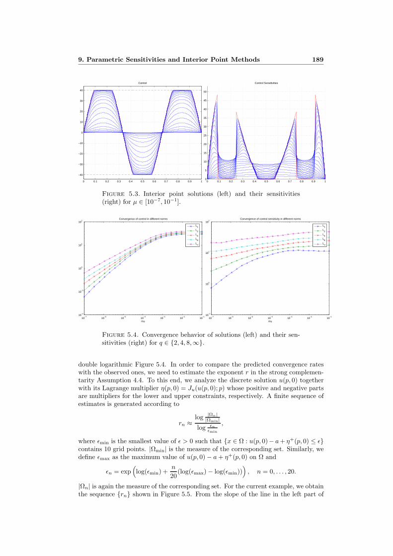
0 0.1 0.2 0.3 0.4 0.5 0.6 0.7 0.8 0.9 1

−40

−30

−20

−10

0

10

20

30

40

Control

0 0.1 0.2 0.3 0.4 0.5 0.6 0.7 0.8 0.9 10

5

10

15

20

25

30

35

40

45

50

Control Sensitivities

Figure 5.3. Interior point solutions (left) and their sensitivities(right) for µ ∈ [10−7, 10−1].

10−7

10−6

10−5

10−4

10−3

10−2

10−1

10−2

10−1

100

101

102

Convergence of control in different norms

mu

L1

L2

L4

L8

L∞

10−7

10−6

10−5

10−4

10−3

10−2

10−1

10−1

100

101

102

Convergence of control sensitivity in different norms

mu

L1

L2

L4

L8

L∞

Figure 5.4. Convergence behavior of solutions (left) and their sen-sitivities (right) for q ∈ 2, 4, 8,∞.

double logarithmic Figure 5.4. In order to compare the predicted convergence rateswith the observed ones, we need to estimate the exponent r in the strong complemen-tarity Assumption 4.4. To this end, we analyze the discrete solution u(p, 0) togetherwith its Lagrange multiplier η(p, 0) = Ju(u(p, 0); p) whose positive and negative partsare multipliers for the lower and upper constraints, respectively. A finite sequence ofestimates is generated according to

rn ≈log |Ωn|

|Ωmin|log ǫn

ǫmin

,

where ǫmin is the smallest value of ǫ > 0 such that x ∈ Ω : u(p, 0)− a+ η+(p, 0) ≤ ǫcontains 10 grid points. |Ωmin| is the measure of the corresponding set. Similarly, wedefine ǫmax as the maximum value of u(p, 0)− a+ η+(p, 0) on Ω and

ǫn = exp(log(ǫmin) +

n

20(log(ǫmax)− log(ǫmin))

), n = 0, . . . , 20.

|Ωn| is again the measure of the corresponding set. For the current example, we obtainthe sequence rn shown in Figure 5.5. From the slope of the line in the left part of


10−4

10−3

10−2

10−1

100

101

102

10−2

10−1

100

Measure of set

ε

Figure 5.5. Sequence of estimates rn for the exponent in the strongcomplementarity assumption.

control control sensitivity state state sensitivityq predicted observed predicted observed observed observed

1 — 0.8403 — 0.4894 0.8731 0.50962 0.7500 0.7136 0.2500 0.2470 0.8739 0.49344 0.6250 0.5961 0.1250 0.1169 0.8739 0.47108 0.5625 0.5387 0.0625 0.0484 0.8765 0.4482∞ 0.5000 0.4978 — — 0.8801 0.4015

Table 5.2. Predicted and observed convergence rates in different Lq

norms for the control and its sensitivity, and observed rates for thestate and its sensitivity.

the figure, we deduce the estimate r = 1. The same result is found for the upperbound.

Table 5.2 shows again the predicted and observed convergence rates for the controland its sensitivity, as well as the observed rates for the state y = Su and its sensitivity.All observed rates are estimated using (5.1) with µ1 and µ2 being the two smallestnonzero values of µ used. Again, the observed convergence rates for the control are ingood agreement with the predicted ones and confirm our analysis for q ∈ [2,∞]. Sincein 1D, the solution operator S is continuous from L1 to L∞, the observed rates for thecontrol in L1 carry over to the state variables in Lq for all q ∈ [2,∞], and likewise tothe adjoint states. Similarly, the L1 rates for the control sensitivity carry over to theLq rates for the state and adjoint sensitivities.

5.3. A Regularized Obstacle Problem. Here we consider the obstacle problem

minu∈H1

0

‖∇u‖2L2+ p〈u, l〉 s.t. u ≥ −1 (5.2)

on Ω = (0, 1)2 ⊂ R2, which, however, does not fit into the theoretical frame set inSection 2. Formally dualizing (5.2) leads to

minη∈H−1

〈η,−∆−1η〉+ p〈η,∆−1l〉 s.t. η ≥ 0,


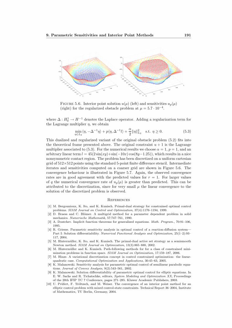
0

0.2

0.4

0.6

0.8

1

00.1

0.20.3

0.40.5

0.60.7

0.80.9

1

−1

−0.5

0

0.5

0

0.2

0.4

0.6

0.8

1

00.1

0.20.3

0.40.5

0.60.7

0.80.9

1

−1

−0.5

0

0.5

Figure 5.6. Interior point solution u(µ) (left) and sensitivities up(µ)(right) for the regularized obstacle problem at µ = 5.7 · 10−4.

where ∆ : H10 → H−1 denotes the Laplace operator. Adding a regularization term for

the Lagrange multiplier η, we obtain

minη∈L2

〈η,−∆−1η〉+ p〈η,∆−1l〉+α

2‖η‖2L2

s.t. η ≥ 0. (5.3)

This dualized and regularized variant of the original obstacle problem (5.2) fits intothe theoretical frame presented above. The original constraint u + 1 is the Lagrangemultiplier associated to (5.3). For the numerical results we choose α = 1, p = 1, and anarbitrary linear term l = 45(2 sin(xy)+sin(−10x) cos(8y−1.25)), which results in a nicenonsymmetric contact region. The problem has been discretized on a uniform cartesiangrid of 512×512 points using the standard 5-point finite difference stencil. Intermediateiterates and sensitivities computed on a coarser grid are shown in Figure 5.6. Theconvergence behaviour is illustrated in Figure 5.7. Again, the observed convergencerates are in good agreement with the predicted values for r = 1. For larger valuesof q the numerical convergence rate of up(µ) is greater than predicted. This can beattributed to the discretization, since for very small µ the linear convergence to thesolution of the discretized problem is observed.

References

[1] M. Bergounioux, K. Ito, and K. Kunisch. Primal-dual strategy for constrained optimal controlproblems. SIAM Journal on Control and Optimization, 37(4):1176–1194, 1999.

[2] D. Braess and C. Blomer. A multigrid method for a parameter dependent problem in solidmechanics. Numerische Mathematik, 57:747–761, 1990.

[3] A. Dontchev. Implicit function theorems for generalized equations. Math. Program., 70:91–106,1995.

[4] R. Griesse. Parametric sensitivity analysis in optimal control of a reaction-diffusion system—Part I: Solution differentiability. Numerical Functional Analysis and Optimization, 25(1–2):93–117, 2004.


[6] M. Hintermuller and K. Kunisch. Path-following methods for for a class of constrained mini-

mization problems in function space. SIAM Journal on Optimization, 17:159–187, 2006.[7] M. Hinze. A variational discretization concept in control constrained optimization: the linear-

quadratic case. Computational Optimization and Applications, 30:45–63, 2005.[8] K. Malanowski. Sensitivity analysis for parametric optimal control of semilinear parabolic equa-

tions. Journal of Convex Analysis, 9(2):543–561, 2002.[9] K. Malanowski. Solution differentiability of parametric optimal control for elliptic equations. In

E. W. Sachs and R. Tichatschke, editors, System Modeling and Optimization XX, Proceedingsof the 20th IFIP TC 7 Conference, pages 271–285. Kluwer Academic Publishers, 2003.

[10] U. Prufert, F. Troltzsch, and M. Weiser. The convergence of an interior point method for anelliptic control problem with mixed control-state constraints. Technical Report 36–2004, Instituteof Mathematics, TU Berlin, Germany, 2004.


0

0.1

0.2

0.3

0.4

0.5

0.6

0.7

0.8

0.9

1 10 100 1000

Figure 5.7. Numerically observed convergence rates of interior pointiterates (top markers) and sensitivities (bottom markers) for differentvalues of q ∈ [1, 1000]. Thin lines denote the analytically predictedvalues.

[11] M. Ulbrich. Semismooth Newton methods for operator equations in function spaces. SIAM Jour-nal on Optimization, 13:805–842, 2003.

[12] M. Ulbrich and S. Ulbrich. Superlinear convergence of affine-scaling interior-point Newton meth-ods for infinite-dimensional nonlinear problems with pointwise bounds. SIAM Journal on Controland Optimization, 38(6):1938–1984, 2000.

[13] M. Vath. Integration Theory. A second course. World Scientific, Singapore, 2002.[14] M. Weiser. Interior point methods in function space. SIAM Journal on Control and Optimization,

44(5):1766–1786, 2005.[15] M. Weiser, T. Ganzler, and A. Schiela. Control reduced primal interior point methods. Report

04-38, ZIB, 2004.

Appendix A. An Implicit Function Theorem

For the sake of easy reference we state here an implicit function theorem which isan adaptation of Theorem [3, Theorem 2.4].

Theorem A.1 (Implicit Function Theorem). Let X be a Banach space and let P,Zbe normed linear spaces. Suppose that G : X × P → Z is a function and N : X → Zis a set-valued map. Let u∗ ∈ X be a solution to

0 ∈ G(u, p) +N(u) (A.1)

for p = p∗, and let W be a neighborhood of 0 ∈ Z. Suppose that(i) G is Lipschitz in p, uniformly in u at (u∗, p∗), and G(u∗, ·) is directionally

differentiable at p∗ with directional deriative Dp(G(u∗, p∗); δp) for all δp ∈ P ,(ii) G is partially Frechet differentiable with respect to u in a neighborhood of

(u∗, p∗), and its partial derivative Gu is continuous in both u and p at (u∗, p∗),(iii) there exists a function ξ : W → X such that ξ(0) = u0, δ ∈ G(u∗, p∗) +

Gu(u∗, p∗)(ξ(δ)− u∗) +N(ξ(δ)) for all δ ∈ W, and ξ is Lipschitz continuous.Then there exist neighborhoods U of u∗ and V of p∗ and a function p 7→ u(p) from Vto U such that u(p∗) = u∗, u(p) is a solution of (A.1) for every p ∈ V , and u(·) isLipschitz continuous.


If in addition, X ⊃ X is a normed linear space such that(iv) ξ : W → X is directionally differentiable at 0 with derivative Dξ(0; δ) for all

δ ∈ Z,then p 7→ u(p) ∈ X is also directionally differentiable at p∗ and the derivative is givenby Dξ(0;−DpG(u∗, p∗; δp)) for all δp ∈ P .

Appendix B. A Saddle Point Lemma

For convenience we state here the saddle point lemma by Braess and Blomer [2,Lemma B.1].

Lemma B.1. Let V and M be Hilbert spaces. Assume the following conditions hold:(1) The continuous linear operator B : V → M∗ satisfies the inf-sup-condition:

There exists a constant β > 0 such that

infζ∈M

supv∈V

〈ζ, Bv〉‖v‖V ‖ζ‖M

≥ β .

(2) The continuous linear operator A : V → V ∗ is symmetric positive definite onthe nullspace of B and positive semidefinite on the whole space V : There existsa constant α > 0 such that

〈v,Av〉 ≥ α‖v‖2V for all v ∈ kerB

and〈v,Av〉 ≥ 0 for all v ∈ V .

(3) The continuous linear operator D : M → M∗ is symmetric positive semi-definite.

Then, the operator [A B∗

B −D]

: V ×M → V ∗ ×M∗

is invertible. The inverse is bounded by a constant depending only on α, β, and thenorms of A, B, and D.


Bibliography

W. Alt. The Lagrange-Newton method for infinite-dimensional optimization problems.Numerical Functional Analysis and Optimization, 11:201–224, 1990.

W. Alt. Local convergence of the Lagrange-Newton method with applications tooptimal control. Control and Cybernetics, 23(1–2):87–105, 1994.

W. Alt, R. Griesse, N. Metla, and A. Rosch. Lipschitz stability for elliptic optimalcontrol problems with mixed control-state constraints. submitted, 2006.

R. Becker and B. Vexler. Mesh refinement and numerical sensitivity analysis forparameter calibration of partial differential equations. Journal of ComputationalPhysics, 206(1):95–110, 2005.

M. Bergounioux, K. Ito, and K. Kunisch. Primal-dual strategy for constrained optimalcontrol problems. SIAM Journal on Control and Optimization, 37(4):1176–1194,1999.

F. Bonnans and A. Shapiro. Perturbation Analysis of Optimization Problems. Springer,Berlin, 2000.

K. Brandes and R. Griesse. Quantitative stability analysis of optimal solutions in PDE-constrained optimization. Journal of Computational and Applied Mathematics, 206(2):908–926, 2007. doi: http://dx.doi.org/10.1016/j.cam.2006.08.038.

E. Casas. Control of an elliptic problem with pointwise state constraints. SIAMJournal on Control and Optimization, 24(6):1309–1318, 1986.

A. Dontchev. Implicit function theorems for generalized equations. MathematicalProgramming, 70:91–106, 1995.

R. Griesse. Lipschitz stability of solutions to some state-constrained elliptic optimalcontrol problems. Journal of Analysis and its Applications, 25:435–455, 2006.

R. Griesse and B. Vexler. Numerical sensitivity analysis for the quantity of interestin PDE-constrained optimization. SIAM Journal on Scientific Computing, 29(1):22–48, 2007.

R. Griesse and S. Volkwein. A primal-dual active set strategy for optimal boundarycontrol of a nonlinear reaction-diffusion system. SIAM Journal on Control and Opti-mization, 44(2):467–494, 2005. doi: http://dx.doi.org/10.1137/S0363012903438696.

R. Griesse and S. Volkwein. Analysis for optimal boundary control for a three-dimensional reaction-diffusion system. Report No. 277, Special Research CenterF003, Project Area II: Continuous Optimization and Control, University of Graz &Technical University of Graz, Austria, 2003.

R. Griesse and S. Volkwein. Parametric sensitivity analysis for optimal boundarycontrol of a 3D reaction-diffusion system. In G. Di Pillo and M. Roma, editors,Large-Scale Nonlinear Optimization, volume 83 of Nonconvex Optimization and itsApplications, pages 127–149, Berlin, 2006. Springer.

R. Griesse and M. Weiser. On the interplay between interior pointapproximation and parametric sensitivities in optimal control. Journalof Mathematical Analysis and Applications, 337(2):771–793, 2008. doi:http://dx.doi.org/10.1016/j.jmaa.2007.03.106.

196 Bibliography

R. Griesse, M. Hintermuller, and M. Hinze. Differential stability of controlconstrained optimal control problems for the Navier-Stokes equations. Nu-merical Functional Analysis and Optimization, 26(7–8):829–850, 2005. doi:http://dx.doi.org/10.1080/01630560500434278.

R. Griesse, N. Metla, and A. Rosch. Local quadratic convergence of SQP for ellipticoptimal control problems with mixed control-state constraints. submitted, 2007.

R. Griesse, T. Grund, and D. Wachsmuth. Update strategies for perturbed nonsmoothequations. Optimization Methods and Software, to appear.

M. Heinkenschloss and F. Troltzsch. Analysis of the Lagrange-SQP-Newton Methodfor the Control of a Phase-Field Equation. Control Cybernet., 28:177–211, 1998.

M. Hintermuller and M. Hinze. An SQP Semi-Smooth Newton-Type Algorithm Ap-plied to the Instationary Navier-Stokes System Subject to Control Constraints.SIAM Journal on Optimization, 16(4):1177–1200, 2006.

M. Hintermuller, K. Ito, and K. Kunisch. The primal-dual active set strategy as asemismooth Newton method. SIAM Journal on Optimization, 13(3):865–888, 2002.

K. Malanowski. Sensitivity analysis for parametric optimal control of semilinear par-abolic equations. Journal of Convex Analysis, 9(2):543–561, 2002.

K. Malanowski. Solution differentiability of parametric optimal control for ellipticequations. In E. W. Sachs and R. Tichatschke, editors, System Modeling and Opti-mization XX, Proceedings of the 20th IFIP TC 7 Conference, pages 271–285. KluwerAcademic Publishers, 2003a.

K. Malanowski. Remarks on differentiability of metric projections onto cones of non-negative functions. Journal of Convex Analysis, 10(1):285–294, 2003b.

K. Malanowski and F. Troltzsch. Lipschitz stability of solutions to parametric optimalcontrol for elliptic equations. Control and Cybernetics, 29:237–256, 2000.

K. Malanowski and F. Troltzsch. Lipschitz stability of solutions to parametric optimalcontrol for parabolic equations. Journal of Analysis and its Applications, 18(2):469–489, 1999.

S. Robinson. Strongly regular generalized equations. Mathematics of Operations Re-search, 5(1):43–62, 1980.

A. Rosch and F. Troltzsch. Existence of regular Lagrange multipliers for a nonlinearelliptic optimal control problem with pointwise control-state constraints. SIAMJournal on Control and Optimization, 45(2):548–564, 2006.

T. Roubıcek and F. Troltzsch. Lipschitz stability of optimal controls for the steady-state Navier-Stokes equations. Control and Cybernetics, 32(3):683–705, 2003.

F. Troltzsch. Lipschitz stability of solutions of linear-quadratic parabolic control prob-lems with respect to perturbations. Dynamics of Continuous, Discrete and ImpulsiveSystems Series A Mathematical Analysis, 7(2):289–306, 2000.

F. Troltzsch. Optimale Steuerung partieller Differentialgleichungen. Vieweg, Wies-baden, 2005.

F. Troltzsch. On the Lagrange-Newton-SQP method for the optimal control of semilin-ear parabolic equations. SIAM Journal on Control and Optimization, 38(1):294–312,1999.

F. Troltzsch and S. Volkwein. The SQP method for control constrained optimal controlof the Burgers equation. ESAIM: Control, Optimisation and Calculus of Variations,6:649–674, 2001.

M. Ulbrich. Semismooth Newton methods for operator equations in function spaces.SIAM Journal on Control and Optimization, 13(3):805–842, 2003.

A. Unger. Hinreichende Optimalitatsbedingungen zweiter Ordnung und Konvergenzdes SQP-Verfahrens fur semilineare elliptische Randsteuerpeobleme. PhD thesis,Chemnitz University of Technology, Germany, 1997.

197

D. Wachsmuth. Regularity and stability of optimal controls of instationary Navier-Stokes equations. Control and Cybernetics, 34:387–410, 2005.

D. Wachsmuth. Analysis of the SQP method for optimal control problems governedby the instationary Navier-Stokes equations based on Lp theory. SIAM Journal onControl and Optimization, 46:1133–1153, 2007.

stability and sensitivity analysis in optimal control of ... · pdf filepreface the topic of...

Documents