stability and optimality in parametric convex programming

Mathematical Communications 6(2001), 107-121 107

Stability and optimality in parametric convexprogramming models∗

R.Trujillo-Cortez†

and S. Zlobec‡

Abstract. Equivalent conditions for structural stability are givenfor convex programming models in terms of three point-to-set mappings.These mappings are then used to characterize locally optimal parameters.For Lagrange models and, in particular, LFS models the characteriza-tions are given relative to general (possibly unstable) perturbations.

Key words: stable convex model, unstable convex model, optimalparameter, Lagrange multiplier function, LFS function

AMS subject classifications: 90C25, 90C31

Received June 4, 2001 Accepted July 20, 2001

1. Introduction

“Stability” and “optimality” are the fundamental notions in optimization andapplied mathematics. Although not uniquely defined, they are often expressedin terms of each other. For example “structural optima” is defined for “stable”perturbations [21], while “stable” models require that the set of optimal solutionsbe non-empty and bounded [18, 19, 20]. This paper studies both stability andoptimality in convex models using three point-to-set mappings.

Stability is essentially defined as lower semi-continuity of the feasible set map-ping. New equivalent conditions for stability are established here using two otherpoint-to-set mappings. The conditions are useful, in particular, when one wantsto know whether the feasible set mapping is continuous for a specific type of per-turbations of specific coefficients. Let us recall that stability, relative to arbitrary

∗Research supported in part by the “Direccion General de Asuntos del Personal Academico”,UNAM, Mexico and the National Science and Engineering Research Council of Canada. The paperwas presented to the Sixth Conference of Approximation and Optimization in the Caribbean heldin Guatemala City, Guatemala, March, 2001.

†Instituto de Matematicas, UNAM, Area de la Investigacion Cientıfica, Circuito Exterior, Ciu-dad Universitaria, Coyoacan 04510, Mexico, D.F. Mexico, e-mail: [email protected]. Contribu-tion of this author is based in part on his Ph.D. thesis at McGill University.

‡Department of Mathematics and Statistics, Burnside Hall, McGill University, Montreal, Que-bec, Canada H3A 2K6, e-mail: [email protected]

108 R.Trujillo-Cortez and S. Zlobec

perturbations of all coefficients in the system is equivalent to the existence of aSlater point, which is also equivalent to the notions of “regularity” [14, 15] and“C-stability”, as recently shown in [17]. These results for linear systems were givenin [8]. For construction of stable perturbations in perturbed linear systems andapplications see [24].

The basic optimality problem in the study of convex parametric models (hence-forth abbreviated: models) is to describe, and possibly calculate, the parametersthat optimize the optimal value function. These parameters have been characterizedfor stable perturbations in [18, 19, 20]. Under “input constraint qualifications” thenecessary conditions for locally optimal parameter are simplified [20]. Some of theoptimality conditions have been recently extended to abstract settings in [1]. Thisextension has many potential applications from dynamic formulations of manage-ment and operations research problems to control theory [4, 7]. Our contributionto the topic of optimality is a characterization of locally optimal parameters in theabsence of stability. We show that such characterization is possible for “Lagrangemodels”. Such models include all convex models for which the constraints have“locally flat surfaces” (the so-called LFS constraints, e.g., [11, 12]) and, in partic-ular, all linear models. It is important to observe that characterizations of locallyoptimal parameters are different for stable and unstable perturbations.

In view of the Liu-Floudas transformation [10], every mathematical programwith twice continuously differentiable functions can be transformed into a partlyconvex program and these can be considered and studied as convex models, e.g.,[22, 23, 25]. This means that our results are applicable to the general optimizationproblems.

2. Stability

Consider the system of perturbed constraints

f i(x, θ) ≤ 0, i ∈ P = {1, . . . , q},A(θ)x = b(θ), (C,θ)

x ≥ 0

where f i : Rn+p −→ R are continuous functions defined (with finite values) on

the entire Rn+p, i ∈ P , A(θ) is an m × n matrix and b(θ) is an m-tuple, both

with elements that are continuous functions of θ ∈ Rp. We assume that f i(·, θ) :

Rn −→ R, i ∈ P , are convex functions for every θ. The vector θ is referred to as

the parameter and x ∈ Rn is the decision variable. As θ varies so does the set of

feasible decisions

F : θ −→ F(θ) = {x ∈ Rn : f i(x, θ) ≤ 0, i ∈ P, A(θ)x = b(θ), x ≥ 0}.

The changes are described by the point-to-set mapping F : Rp −→ R

n defined asF : θ −→ F(θ). With every point (vector) θ, the mapping F associates the feasibleset F(θ). The set of all θ’s for which F(θ) is not empty is called the feasible set ofparameters and it is denoted by F = {θ : F(θ) �= ∅}. As θ ∈ F varies so do many

Stability and optimality in parametric convex programming 109

other objects that can be described by point-to-set mappings. These include theindex mappings

P= : θ −→ P

=(θ) = {i ∈ P : x ∈ F(θ) ⇒ f i(x, θ) = 0}

andN

= : θ −→ N=(θ) = {i ∈ N : x ∈ F(θ) ⇒ xi = 0}

where N = {1, . . . , n}. By analogy with the terminology used in [20, 24], for everyθ, we call these indices, respectively, the minimal index set of inequality constraintsand the minimal index set of variables. We will also use F= : θ −→ F=(θ) where

F=(θ) = {x : f i(x, θ) = 0, i ∈ P=(θ), A(θ)x = b(θ), xj = 0, j ∈ N

=(θ)}.

This mapping is used in characterizations of optimal variables, e.g., [3, 18, 25].Stability of a system of constraints and optimality of parameters will be studiedaround an arbitrary but fixed θ� ∈ F. For this purpose we also need F=

� : θ −→ F=� (θ)

where

F=

� (θ) = {x : f i(x, θ) ≤ 0, i ∈ P=(θ�), A(θ)x = b(θ), xj ≥ 0, j ∈ N

=(θ�)}.

This mapping is also important in the study of Lagrange multiplier functions, e.g.,[18, 25]. Let us recall how lower semi-continuity of a general point-to-set mappingΓ : R

p −→ Rn is defined (see, e.g., [2, 5, 9]): The mapping Γ is lower semi-continuous

at θ� ∈ Rp if for each open set A ⊂ R

n, satisfying A ∩ Γ(θ�) �= ∅, there exists aneighborhood N(θ�) of θ� such that A ∩ Γ(θ) �= ∅ for each θ ∈ N(θ�).

Definition 1. The perturbed convex system (C,θ) is said to be structurallystable at θ� ∈ F if the point-to-set mapping F : θ −→ F(θ) is lower semi-continuousat θ�.

Remark 1. It is well known that Γ is lower semi-continuous if, and only if, itis open. Since the mapping F is closed, F is continuous if, and only if, it is lowersemi-continuous.

In mathematical programming models describing real-life situations not neces-sarily all coefficients are perturbed. Typically, one wants to study the effect ofsome specific perturbations on the system. For example, one may be interested inhow changes of certain technological coefficients in linear programs influence thesystem. In this case θ = θ(t) can be specified to be one or more elements suchas θ = (a1,2, a4,3, b2). It is also meaningful to talk only about perturbations thatpreserve lower semi-continuity of the feasible set mapping. In this case we mayrestrict the notion of lower semi-continuity and structural stability to only a partof the neighborhood. Following [19, 20] we say that the mapping is lower semi-continuous at θ� ∈ R

p, relative to a set S that contains θ�, if for each open setA ⊂ R

n, satisfying A ∩ Γ(θ�) �= ∅, there exists a neighborhood N(θ�) of θ� suchthat A ∩ Γ(θ) �= ∅ for each θ ∈ N(θ�) ∩ S. We also say that the system (C,θ) isstructurally stable at θ� ∈ F, relative to a set S that contains θ�, if F : θ −→ F(θ)is lower semi-continuous at θ� relative to S. Such S is called a region of stability atθ�, e.g., [18, 25]. For the sake of simplicity we assume, throughout the paper, thatS is a connected set.


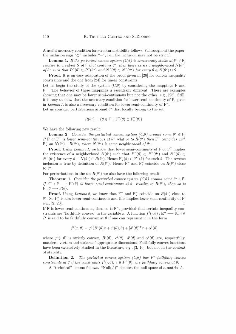
A useful necessary condition for structural stability follows. (Throughout the paper,the inclusion sign “⊂” includes “=”, i.e., the inclusion may not be strict.)

Lemma 1. If the perturbed convex system (C,θ) is structurally stable at θ� ∈ F,relative to a subset S of F that contains θ�, then there exists a neighborhood N(θ�)of θ� such that P

=(θ) ⊂ P=(θ�) and N

=(θ) ⊂ N=(θ�) for every θ ∈ N(θ�) ∩ S.

Proof. It is an easy adaptation of the proof given in [20] for convex inequalityconstraints and the one from [24] for linear constraints. ✷

Let us begin the study of the system (C,θ) by considering the mappings F andF=. The behavior of these mappings is essentially different. There are examplesshowing that one may be lower semi-continuous but not the other, e.g., [25]. Still,it is easy to show that the necessary condition for lower semi-continuity of F, givenin Lemma1, is also a necessary condition for lower semi-continuity of F=.Let us consider perturbations around θ� that locally belong to the set

R(θ�) = {θ ∈ F : F=(θ) ⊂ F=

� (θ)}.

We have the following new result:Lemma 2. Consider the perturbed convex system (C,θ) around some θ� ∈ F.

If F or F= is lower semi-continuous at θ� relative to R(θ�) then F= coincides withF=

� on N(θ�) ∩R(θ�), where N(θ�) is some neighborhood of θ�.Proof. Using Lemma1, we know that lower semi-continuity of F or F= implies

the existence of a neighborhood N(θ�) such that P=(θ) ⊂ P=(θ�) and N=(θ) ⊂N

=(θ�) for every θ ∈ N(θ�) ∩R(θ�). Hence F=� (θ) ⊂ F=(θ) for such θ. The reverse

inclusion is true by definition of R(θ�). Hence F= and F=� coincide on R(θ�) close

to θ�. ✷

For perturbations in the set R(θ�) we also have the following result:Theorem 1. Consider the perturbed convex system (C,θ) around some θ� ∈ F.

If F= : θ −→ F=(θ) is lower semi-continuous at θ� relative to R(θ�), then so isF : θ −→ F(θ).

Proof. Using Lemma 2, we know that F= and F=� coincide on R(θ�) close to

θ�. So F=� is also lower semi-continuous and this implies lower semi-continuity of F;

e.g., [2, 20]. ✷

If F is lower semi-continuous, then so is F=, provided that certain inequality con-straints are “faithfully convex” in the variable x. A function f i(·, θ) : R

n −→ R, i ∈P, is said to be faithfully convex at θ if one can represent it in the form

f i(x, θ) = ϕi(Bi(θ)x + ci(θ), θ) + [di(θ)]Tx + αi(θ)

where ϕi(·, θ) is strictly convex, Bi(θ), ci(θ), di(θ) and αi(θ) are, respectfully,matrices, vectors and scalars of appropriate dimensions. Faithfully convex functionshave been extensively studied in the literature, e.g., [3, 16], but not in the contextof stability.

Definition 2. The perturbed convex system (C,θ) has P=-faithfully convex

constraints at θ if the constraints f i(·, θ), i ∈ P=(θ), are faithfully convex at θ.

A “technical” lemma follows. “Null(A)” denotes the null-space of a matrix A.


Lemma 3. Consider the perturbed convex system (C,θ) with P=-faithfully con-

vex constraints at some θ ∈ F. If x ∈ F=(θ) and y ∈ F(θ), then

x− y ∈ Null

⋂

i∈P=(θ)

[Bi(θ)

(di(θ))T

] .

Proof. Since F(θ) ⊂ F=(θ) and F=(θ) is a convex set, it follows that x + α(y −x) ∈ F=(θ) for all α ≥ 0 sufficiently small. Hence f i(x+α(y−x), θ) = 0, i ∈ P

=(θ).This means that y− x is in the cone of directions of constancy of f i(·, θ) at x (e.g.,[3, 25]). But the latter, for faithfully convex functions, is the null-space of thematrix [[Bi(θ)]T, di(θ)]T, e.g., [3]. (An alternative proof of this lemma is given in[17].) ✷

The following result was proved for linear systems in [6]. We prove it here forP=-faithfully convex constraints.

Theorem 2. Consider the perturbed convex system (C,θ) around some θ� ∈ Fand some subset S of F that contains θ�. Assume that the system has P

=-faithfullyconvex constraints at every θ ∈ S. If F is lower semi-continuous at θ� relative toS, then so is F=.

Proof. Take an x� ∈ F=(θ�) and a sequence θk ∈ S. There exists a y ∈ F(θ�)such that

f i(y, θ�) < 0, i ∈ P \ P=(θ�),

A(θ�)y = b(θ�),yi > 0, i ∈ N \N

=(θ�).

Hence there exists 0 < ε < 1 such that z = y + ε(x� − y) satisfies

f i(z, θ�) < 0, i ∈ P \ P=(θ�),

A(θ�)z = b(θ�), because A(θ�)x� = b(θ�),zi > 0, i ∈ N \N

=(θ�).

Also, by convexity, we have

f i(z, θ�) ≤ (1− ε)f i(y, θ�) + εf i(x�, θ�) ≤ 0, i ∈ P=(θ�),

zi = (1− ε)yi + εx�

i ≥ 0, i ∈ N=(θ�).

This means that z ∈ F(θ�). Since F is lower semi-continuous, there exist sequencesyk ∈ F(θk), yk −→ y and zk ∈ F(θk), zk −→ z. For the same ε construct the newsequence xk = yk + (zk−yk)

ε . Clearly xk −→ x�. In order to complete the proofwe have to show that xk ∈ F=(θk) for large k’s. This is true because, for every


i ∈ P=(θk), we have

f i(xk, θk) = ϕi(Bi(θk)[yk +(zk − yk)

ε] + ci(θk), θk) + [di(θk)]T[yk +

(zk − yk)ε

]

+ αi(θk)

= ϕi(Bi(θk)yk + ci(θk), θk) + [di(θk)]Tyk + αi(θk), by Lemma 3,

= f i(yk, θk), by definition,

= 0, because yk ∈ F(θk) ⊂ F=(θk).

AlsoA(θk)xk = b(θk), since A(θk)yk = A(θk)zk = b(θk).

Finally, since F is lower semi-continuous, for every large k, we have N=(θk) ⊂

N=(θ�) and hence yk

i = zki = 0, i ∈ N

=(θk). ✷

The faithful convexity is a crucial assumption in Theorem 2. Without it the theoremdoes not hold. This is confirmed by the next example.

Example 1. Consider the system

f(x, θ) ≤ 0, 0 ≤ x ≤ 1

where f(x, θ) = θ2(|x| − 1), if |x| > 1, and 0 otherwise. Here F(θ) is the same forevery θ and hence F is lower semi-continuous at θ� = 0. But F=(θ) = R for θ = θ�,and −1 ≤ x ≤ 1 otherwise. Hence F= is not lower semi-continuous. Note that theconstraint f is not faithfully convex at θ �= θ�. ✷

Let us now include the mapping F=� in our study. Lower semi-continuity of this

mapping is required in many statements related to input constraint qualifications,optimality conditions, and Lagrange multiplier functions; e.g., [18, 19, 20]. It isused to characterize structurally stable convex and linear systems; e.g., [18, 20].(See also Theorem 6 below.) The mappings F= and F=

� coincide for the system in-troduced in Example 1 but generally these mappings are different. The assumptionsof Theorem 2 alone do not guarantee that F=

� is lower semi-continuous. However,this is the case if perturbations are restricted to the set R(θ�):

Theorem 3. Consider the perturbed convex system (C,θ) around some θ� ∈ F.Assume that the system has P

=-faithfully convex constraints at every θ ∈ R(θ�). IfF is lower semi-continuous at θ� relative to R(θ�), then so is F=

�.Proof. Again, using Lemma 2, we have that F= and F=

� coincide on R(θ�) closeto θ�. The proof now follows from Theorem 2. ✷

Finally, let us now focus on the mappings F=� and F=. If the former is lower semi-

continuous then so is the latter:Theorem 4. Consider the perturbed convex system (C,θ) around some θ� ∈ F.

If F=

� is lower semi-continuous at θ� then so is F=.Proof. Take an open set A such that A ∩ F=(θ�) �= ∅. Since F=(θ�) = F=

� (θ�),also A ∩ F=

� (θ�) �= ∅. But lower semi-continuity of F=� implies that so is F; e.g.,

[2, 20]. Hence P=(θ) ⊂ P

=(θ�) and N=(θ) ⊂ N

=(θ�) for every θ ∈ N(θ�), byLemma1. This further implies F=

� (θ) ⊂ F=(θ) and hence A ∩ F=(θ) �= ∅ for everyθ ∈ N(θ�). ✷


The lower semi-continuity implications between the three mappings, proved in thissection, are depicted in Figure 1. They are stated at an arbitrary but fixed θ� ∈ F.The signs, if any, along an arrow denote the assumptions that are needed in theproof of the implications. Thus “fc=” stands for the assumption that the system(C,θ) has P=-faithfully convex constraints at every perturbation θ, while “R” meansthat the implication holds relative to the set R(θ�). Since lower semi-continuity isa local property, only perturbations in some neighborhood of θ� are considered.

Figure 1. Lower semi-continuity implications

3. Optimality

So far, we have studied perturbed systems of constraints. Now we include an ob-jective function in the study. Consider the convex parametric programming model

min(x)

f(x, θ)

s.t.(P,θ)

f i(x, θ) ≤ 0, i ∈ P = {1, . . . , q}.For the sake of simplicity we only consider inequality constraints in this section.The objective function f and all the constraints f i : R

n+p −→ R are assumed tobe continuous functions defined (with finite values) on the entire R

n+p, i ∈ P . Itis assumed that f(·, θ), f i(·, θ) : R

n −→ R, i ∈ P , are convex functions for everyθ. The notation related to the new formulation is easily adjusted. For instance,given θ, the feasible set is F(θ) = {x ∈ R

n : f i(x, θ) ≤ 0, i ∈ P}. Notation forthe feasible set of parameters F and for the minimal index set of active constraintsP

=(θ) remains the same, while F=(θ) = {x ∈ Rn : f i(x, θ) = 0, i ∈ P

=(θ)} andF=

� (θ) = {x ∈ Rn : f i(x, θ) ≤ 0, i ∈ P=(θ�)} around an arbitrary but fixed θ� ∈ F.

A new point-to-set player is the mapping

Fo : θ −→ Fo(θ) = {xo(θ)}


where xo(θ) denotes an optimal solution of the convex (fixed θ) program (P,θ).(This mapping associates, with every θ, the set of all optimal solutions.) Withthe introduction of the objective function we also have the optimal value functionfo(θ) = f(xo(θ), θ). The main objective of this section is to characterize parametersθ that locally minimize the function fo(θ):

Definition 3. Consider the convex model (P,θ). A parameter θ� ∈ F is a locallyoptimal parameter if fo(θ�) ≤ fo(θ) for every θ ∈ N(θ�) ∩ F, where N(θ�) is someneighborhood of θ�.

Locally optimal parameters can be characterized using the Lagrangian

L(x, u; θ) = f(x, θ) +∑i∈P

uifi(x, θ).

Given θ ∈ F we say that (x�, u�), x� ∈ Rn, u� ∈ R

q, u� ≥ 0, is a saddle point ofthe Lagrangian if

L(x�, u; θ) ≤ L(x�, u�; θ) ≤ L(x, u�; θ)

for every x ∈ Rn and every u = (ui), ui ≥ 0, i ∈ P . It is well known that the set of

all multipliers u� = uo(θ) is the same at every optimal solution x� = xo(θ). Hencewe can study the point-to-set mapping

L : θ −→ L(θ) = {uo(θ)}.Definition 4. Consider the convex model (P,θ) and some subset S of F. If at

every θ ∈ S there exists an optimal solution xo(θ) and if L(θ) �= ∅, then the modelis said to be a Lagrange model on S.

There are convex models that are not Lagrange at any θ ∈ F. The next exampleillustrates a model that is a Lagrange model at only one parameter.

Example 2. Consider

min(x1,x2,x3)

x1 − θx3

s.t.(NL,θ)

(x1 − 1)2 + (x2 − 1)2 − 1 ≤ 0,

(x1 − 1)2 + (x2 + 1)2 − 1 ≤ 0,

−(1 + θ2)x1 + x3 ≤ 0,−x3 ≤ 0.

One can show that this is a Lagrange model only at the root of θ3+θ = 1 (call it θ�).The optimal value function here is fo(θ) = 1 − θ3 − θ, for θ ≥ 0, and 1 otherwise.The feasible set mapping is lower semi-continuous around θ�. Indeed, one can findthat F(θ) = {(1, 0, x3)T ∈ R

3 : 0 ≤ x3 ≤ 1 + θ2}. Later we will check, using anoptimality condition, that θ� is an optimal parameter relative to the set (−∞, θ�].✷

For Lagrange models one can characterize locally optimal parameters withoutrequiring any stability assumption.

Theorem 5. (Characterization of Local Optimality for Lagrange Models Re-lative to Arbitrary Perturbations.) Consider the convex model (P,θ). Assume that


(P,θ) is a Lagrange model on some nonempty set S ⊂ Rp. Take θ� ∈ S and let x� be

an optimal solution of the program (P,θ�). Then θ� is a locally optimal parameterof fo relative to S if, and only if, there exists a neighborhood N(θ�) of θ� such that,for every θ in N(θ�) ∩ S, there exists an element uo(θ) in L(θ) such that

L(x�, u; θ�) ≤ L(x�, uo(θ�); θ�) ≤ L(x, uo(θ); θ) (LSP)

for all x in Rn and all u = (ui), ui ≥ 0, i ∈ P .

Proof. Let us first prove the necessity part first. We know that θ� is a locallyoptimal parameter of fo relative to S, so there exists a neighborhood N(θ�) of θ�

such thatfo(θ�) ≤ fo(θ) for all θ ∈ N(θ�) ∩ S.

Since L(θ�) �= ∅, we have

fo(θ�) = f(x�, θ�) = L(x�, uo(θ�); θ�) for all uo(θ�) ∈ L(θ�).

So

L(x�, uo(θ�); θ�) = fo(θ�) ≤ fo(θ) (3.1)

for all θ in N(θ�)∩S and all uo(θ�) in L(θ�). Now, since (P,θ) is a Lagrange modelon N(θ�)∩S, we know that, for every θ ∈ N(θ�)∩S, there exist an optimal solutionxo(θ) ∈ Fo(θ) and an element uo(θ) in L(θ) such that

fo(θ) = f(xo(θ), θ)= L(xo(θ), uo(θ); θ)≤ L(x, uo(θ); θ) for all x ∈ R

n.

Thus, using (3.1), we conclude that

L(x�, uo(θ�); θ�) ≤ L(x, uo(θ); θ) for all x ∈ Rn.

The left-hand side of the “Lagrange saddle point inequality” (LSP) follows by thefact that x� is a feasible point of (P,θ�).Now, let us prove the sufficiency part. We are going to prove that θ� is a locallyoptimal parameter of fo on the set N(θ�)∩S. Take an arbitrary θ in N(θ�)∩S. Takea saddle point uo(θ�) in L(θ�) and use the left-hand side of (LSP) with u = 0 to getL(x�, uo(θ�); θ�) ≥ 0. By feasibility of the point x� we also have L(x�, uo(θ�); θ�) ≤ 0.Thus ∑

i∈P

uoi(θ

�)f i(x�, θ�) = 0

and consequently, using the right-hand side of (LSP), we get

f(x�, θ�) ≤ f(x, θ) +∑i∈P

uoi(θ)f

i(x, θ)


for some uo(θ) in L(θ) and all x in Rn. In particular

f(x�, θ�) ≤ f(x, θ) +∑i∈P

uoi(θ)f

i(x, θ) ≤ f(x, θ) for all x ∈ F(θ).

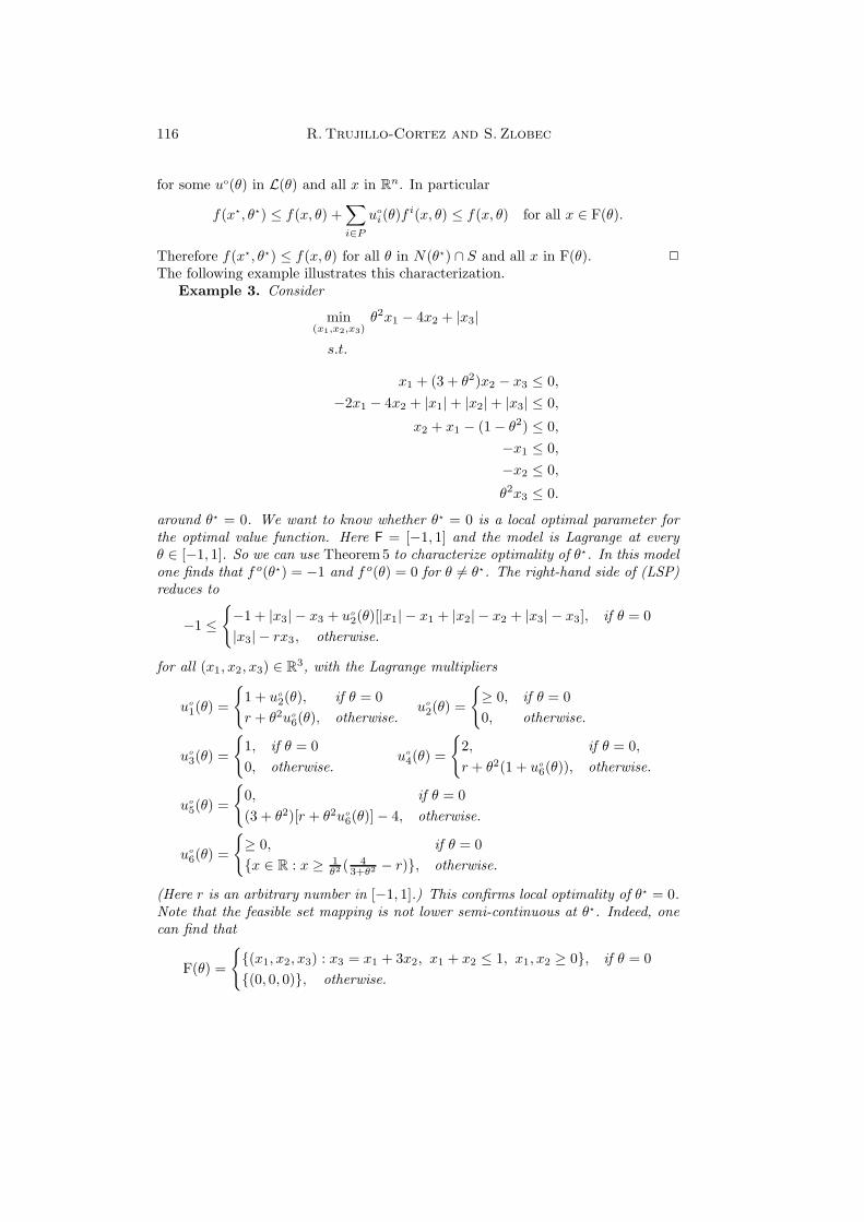
Therefore f(x�, θ�) ≤ f(x, θ) for all θ in N(θ�) ∩ S and all x in F(θ). ✷

The following example illustrates this characterization.Example 3. Consider

min(x1,x2,x3)

θ2x1 − 4x2 + |x3|

s.t.

x1 + (3 + θ2)x2 − x3 ≤ 0,−2x1 − 4x2 + |x1| + |x2|+ |x3| ≤ 0,

x2 + x1 − (1− θ2) ≤ 0,−x1 ≤ 0,−x2 ≤ 0,

θ2x3 ≤ 0.

around θ� = 0. We want to know whether θ� = 0 is a local optimal parameter forthe optimal value function. Here F = [−1, 1] and the model is Lagrange at everyθ ∈ [−1, 1]. So we can use Theorem5 to characterize optimality of θ�. In this modelone finds that fo(θ�) = −1 and fo(θ) = 0 for θ �= θ�. The right-hand side of (LSP)reduces to

−1 ≤{−1 + |x3| − x3 + uo

2(θ)[|x1| − x1 + |x2| − x2 + |x3| − x3], if θ = 0|x3| − rx3, otherwise.

for all (x1, x2, x3) ∈ R3, with the Lagrange multipliers

uo

1(θ) =

{1 + uo

2(θ), if θ = 0r + θ2uo

6(θ), otherwise.uo

2(θ) =

{≥ 0, if θ = 00, otherwise.

uo

3(θ) =

{1, if θ = 00, otherwise.

uo

4(θ) =

{2, if θ = 0,r + θ2(1 + uo

6(θ)), otherwise.

uo

5(θ) =

{0, if θ = 0(3 + θ2)[r + θ2uo

6(θ)] − 4, otherwise.

uo

6(θ) =

{≥ 0, if θ = 0{x ∈ R : x ≥ 1

θ2 ( 43+θ2 − r)}, otherwise.

(Here r is an arbitrary number in [−1, 1].) This confirms local optimality of θ� = 0.Note that the feasible set mapping is not lower semi-continuous at θ�. Indeed, onecan find that

F(θ) =

{{(x1, x2, x3) : x3 = x1 + 3x2, x1 + x2 ≤ 1, x1, x2 ≥ 0}, if θ = 0{(0, 0, 0)}, otherwise.


This means that the results from, e.g., [19, 20], are not applicable here.How to check optimality for the models that are not Lagrange? In particular,

Theorem 5 cannot be applied to the convex model given in Example 2 to checkwhether θ� is an optimal parameter relative to the set (−∞, θ�]. For this kind ofmodels one could check optimality of the parameters using a result given in, e.g.,[18, 19, 20]. That result can be applied to general convex models (not necessarilyLagrange), but it requires stable perturbations. Let us recall this characterization.We denote the cardinality of P< (θ�) = P \ P

=(θ�) by c = card(P< (θ�)). Withoutloss of generality, we assume that P

< (θ�) = {1, . . . , c}. In this case, to test localoptimality for the convex model (P,θ) on some set S containing θ�, we can use the“reduced” Lagrangian function

L<

� (x, u, w; θ) = f(x, θ) +∑

i∈P < (θ�)

uifi(x, θ).

Such a characterization also requires that objective function of the convex model(P,θ) be “realistic” (see, e.g., [20]):

Definition 5. Consider the convex model (P,θ) around some θ� ∈ F. Theobjective function is said to be realistic at θ� if Fo(θ�) �= ∅ and bounded.

In the following result, borrowed from [18], we denote Rc+ = {x ∈ R

c : x ≥ 0}.Theorem 6. (Characterization of Local Optimality for Arbitrary Models on

a Region of Stability.) Consider the convex model (P,θ) with a realistic objectivefunction f at some θ� in F. Let x� be an optimal solution of the program (P,θ�)and let S be a subset of F containing θ�. Assume that the mapping F is lower semi-continuous at θ� relative to S. Then θ� is a locally optimal parameter of fo relativeto S if, and only if, there exists a neighborhood N(θ�) of θ� and a non-negativevector function u� : N(θ�) ∩ S −→ R

c+ such that

L<

� (x�, u; θ�) ≤ L<

� (x�, u�(θ�); θ�) ≤ L<

� (x, u�(θ); θ) (SSP)

for all θ in N(θ�) ∩ S, u in Rc+ and all x in F=

�(θ).Note that (P,θ) is not assumed to be a Lagrange model in this characterization,

but the price we have to pay is lower semi-continuity of F at θ�. Now, we applythis result to the model given in Example 2.

Example 4. Consider the model given in Example 2. The model is not Lagrangearound θ� (the root of θ3 + θ = 1), but it is stable at θ�. Hence Theorem6 applies.We have P

=(θ) = {1, 2} and F=

�(θ) = {(1, 0, x3) ∈ R3 : x3 ∈ R} for every θ ∈ R.

The right-hand side of the “stable saddle point inequality” (SSP) is

0 ≤ x1 − θx3 + u�

3(θ)[−(1 + θ)x1 + x3] + u�

4(θ)[−x3]

for all (x1, x2, x3) ∈ F=

�(θ). It holds, for every θ ∈ (−∞, θ�], with

u�

3(θ) = {u�

3 ∈ R : max{θ, 0} ≤ u�

3 ≤ 11 + θ2

} and u�

4(θ) = u�

3(θ) − θ.

Hence θ� is locally optimal for θ ≤ θ�.It is clear that we cannot use Theorem 6 to check optimality of the parame-

ter θ� = 0 for the model given in Example 3 because the feasible set mapping F,associated to that model, is not lower semi-continuous at θ� = 0.


Remark 2. One can replace the usual Lagrangian L in Theorem5 by the reducedLagrangian L

<

� from Theorem6.If a convex model is not a Lagrange model and if it is unstable at θ�, then none ofthe above characterizations works. One can see this using the example from, e.g.,[1, Example 5.4].

4. Optimality in LFS Models

We have seen in the preceding section that one can characterize locally optimalparameters in convex Lagrange models (regardless of whether perturbations arestable or not). In this section we will show that there is a class of easily identifiableLagrange models. These are models whose constraint functions have “locally flatsurfaces” at every θ. (They are also known as “LFS models”.) We recall these func-tions from [11, 12]. First, given a function f : R

n −→ R, the cones of directions ofconstancy, non-ascent and descent of f at a given x� ∈ R

n are defined, respectively,by

D=f (x�) = {d ∈ R

n : ∃ α0 such that f(x� + αd) = f(x�), 0 < α < α0},D�

f(x�) = {d ∈ R

n : ∃ α0 such that f(x� + αd) � f(x�), 0 < α < α0}

and

D<

f(x�) = {d ∈ R

n : ∃ α0 such that f(x� + αd) < f(x�), 0 < α < α0}.

We recall that the directional derivative of a function f : Rn −→ R at x� ∈ R

n inthe direction d ∈ R

n is

f ′(x�; d) = limλ−→0+

f(x� + λd) − f(x�)λ

.

It is well known that for a convex function f : Rn −→ R the directional derivative

exists for any direction d and any point x� ∈ Rn (see, e.g., [16]). The following

definition was introduced in [11, 12].Definition 6. A convex function f : R

n −→ R is said to have a locally flatsurface at x� ∈ R

n if

D�f (x�) is polyhedral when D<

f(x�) �= ∅, or if

D=f (x�) = {d ∈ R

n : f ′(x�; d) = 0} and polyhedral when D<f (x�) = ∅.

We refer to such a function as an LFS function or a function having the LFSproperty. Such functions are, for example, all linear functions f(x) = aTx + α,a ∈ R

n, α ∈ R, at every x ∈ Rn. So is the l1-norm ‖x‖1 = |x1| + |x2| + . . . + |xn|,

f(x) = aTx + ‖x‖1, at every x ∈ Rn, the exponential function et at every t ∈ R,

etc. Now, we introduce the LFS models.Definition 7. Consider the convex model (P,θ) and some subset S of F. If at

every θ ∈ S there exists an optimal solution xo(θ) such that f i(·, θ) : Rn −→ R, i ∈

P , is LFS at xo(θ), then (P,θ) is called an LFS model on S.


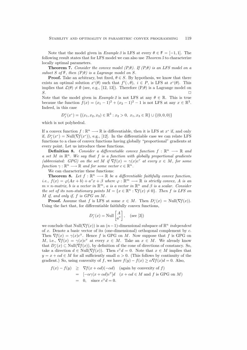
Note that the model given in Example 3 is LFS at every θ ∈ F = [−1, 1]. Thefollowing result states that for LFS model we can also use Theorem 5 to characterizelocally optimal parameters.

Theorem 7. Consider the convex model (P,θ). If (P,θ) is an LFS model on asubset S of F, then (P,θ) is a Lagrange model on S.

Proof. Take an arbitrary, but fixed, θ ∈ S. By hypothesis, we know that thereexists an optimal solution xo(θ) such that f i(·, θ), i ∈ P , is LFS at xo(θ). Thisimplies that L(θ) �= ∅ (see, e.g., [12, 13]). Therefore (P,θ) is a Lagrange model onS. ✷

Note that the model given in Example 2 is not LFS at any θ ∈ R. This is truebecause the function f(x) = (x1 − 1)2 + (x2 − 1)2 − 1 is not LFS at any x ∈ R

3.Indeed, in this case

D�f(x�) = {(x1, x2, x3) ∈ R

3 : x2 > 0, x1, x3 ∈ R} ∪ {(0, 0, 0)}which is not polyhedral.

If a convex function f : Rn −→ R is differentiable, then it is LFS at x� if, and only

if, D=f (x�) = Null(∇f (x�)), e.g., [12]. In the differentiable case we can relate LFS

functions to a class of convex functions having globally “proportional” gradients atevery point. Let us introduce these functions.

Definition 8. Consider a differentiable convex function f : Rn −→ R and

a set M in Rn. We say that f is a function with globally proportional gradients

(abbreviated: GPG) on the set M if ∇f(x) = γ(x)cT at every x ∈ M , for somefunction γ : R

n −→ R and for some vector c ∈ Rn.

We can characterize these functions:Theorem 8. Let f : R

n −→ R be a differentiable faithfully convex function,i.e., f(x) = ϕ(Ax + b) + aTx + β where ϕ : R

m −→ R is strictly convex, A is anm× n-matrix, b is a vector in R

m, a is a vector in Rn and β is a scalar. Consider

the set of its non-stationary points M = {x ∈ Rn : ∇f(x) �= 0}. Then f is LFS on

M if, and only if, f is GPG on M .Proof. Assume that f is LFS at some x ∈ M . Then D=

f (x) = Null(∇f(x)).Using the fact that, for differentiable faithfully convex functions,

D=f (x) = Null

[AaT

], (see [3])

we conclude that Null(∇f(x)) is an (n−1)-dimensional subspace of Rn independent

of x. Denote a basic vector of its (one-dimensional) orthogonal complement by c.Then ∇f(x) = γ(x)cT. Hence f is GPG on M . Now suppose that f is GPG onM , i.e., ∇f(x) = γ(x)cT at every x ∈ M . Take an x ∈ M . We already knowthat D=

f (x) ⊂ Null(∇f(x)), by definition of the cone of directions of constancy. So,take a direction d ∈ Null(∇f(x)). Then cTd = 0. Note that x ∈ M implies thaty = x + αd ∈ M for all sufficiently small α > 0. (This follows by continuity of thegradient.) So, using convexity of f , we have f(y)− f(x) ≥ α∇f (x)d = 0. Also,

f(x) − f(y) ≥ ∇f(x + αd)(−αd) (again by convexity of f)= [−αγ(x + αd)cT]d (x + αd ∈ M and f is GPG on M)= 0, since cTd = 0.


Hence f(x) = f(y) = f(x+αd), i.e., d ∈ D=f (x). This means that f is LFS at x. ✷

5. Conclusions

In view of Section 2 (Figure 1) we have given three equivalent definitions of struc-turally stable convex systems. Then we have observed that optimality conditionsare different in the presence of stability and in its absence. Characterizations oflocally optimal parameters relative to stable perturbations do exist in the litera-ture for convex programming models. Here characterizations are given for generalperturbations (not necessary stable) but only for Lagrange models. In particular,all LFS and linear models are Lagrange models. It remains an open question howto characterize locally optimal parameters for general convex models relative togeneral perturbations.

References

[1] M.Asgharian, S. Zlobec, Convex parametric programming in abstractspaces, Tech. rep., Department of Mathematics and Statistics, McGill Uni-versity, June 2000., to be published.

[2] B.Bank, J.Guddat, D.Klatte, B.Kummer, K.Tammer, Non-LinearParametric Optimization, Akademie-Verlag, Berlin, 1982.

[3] A.Ben-Israel, A.Ben-Tal, S. Zlobec, Optimality in Nonlinear Program-ming: A Feasible Direction Approach, Wiley-Interscience, New York, 1984.

[4] A.Bensoussan, P.Kleindorfer, Ch. S. Tapiero (Eds.), Applied OptimalControl, Studies in the Management Sciences, vol. 9, Kluwer Academic, Ams-terdam: North Holand, 1978.

[5] C.Berge, Topological Spaces, Oliver and Boyd, London, 1963.

[6] M.J.Canovas, M.A.Lopez, J. Parra, Stability of the feasible set for li-near inequality systems: A carrier index set approach, Tech. rep., Departmentof Statistics and Operations Research, University of Alicante, Alicante, Spain,January 2000., to be published.

[7] M.M.Connors, D.Teichroew, Optimal Control of Dynamic OperationsResearch Models, Scranton, Penn: Int. Textbook Company, 1967.

[8] M.A.Goberna, M.A.Lopez, M.Todorov, Stability theory for linear in-equality systems, SIAM Journal on Matrix Analysis and Applications 17(1996),730–743.

[9] W.W.Hogan, Point-to-set maps in mathematical programming, SIAM15(1973), 591–603.

[10] W.B. Liu, C.A.Floudas, A remark on the GOP algorithm for global opti-mization, Journal of Global Optimization 3(1993), 519–521.


[11] S. F.Mokhtarian, Mathematical Programming with LFS Functions, Master’sthesis, Department of Mathematics and Statistics, McGill University, Mon-treal, 1992.

[12] S. F.Mokhtarian, S. Zlobec, LFS functions in nonsmooth programming,Utilitas Mathematica 45(1994), 3–15.

[13] L.Neralic, S. Zlobec, LFS functions in multi-objective programming, Ap-plications of Mathematics 41(1996), 347–366.

[14] S.M.Robinson, Stability theory for system of inequalities, Part I: Linear sys-tems, SIAM Journal on Numerical Analysis 12(1975), 754–769.

[15] S.M.Robinson, Stability theory for system of inequalities, Part II: Differ-entiable nonlinear systems, SIAM Journal on Numerical Analysis 13(1976),497–513.

[16] T. Rockafellar, Convex Analysis, Princeton University Press, New Jersey,1970.

[17] R. Trujillo-Cortez, Stable Convex Parametric Programming and Applica-tions, PhD thesis, Department of Mathematics and Statistics, McGill Univer-sity, Montreal, 2000.

[18] M.Van Rooyen, S. Zlobec, A complete characterization of optimal eco-nomic systems with respect to stable perturbations, Glasnik Matematicki25(1990), 235–253.

[19] S. Zlobec, Input optimization: I. Optimal realizations of mathematical mod-els, Mathematical Programming 31(1985), 245–268.

[20] S. Zlobec, Characterizing optimality in mathematical programming models,Acta Applicandae Mathematicae 12(1988), 113–180.

[21] S. Zlobec, Structural optima in nonlinear programming, In: Advances inMathematical Optimization, (J.Guddat, et al., eds.), vol. 45. Kluwer Acad-emic, Berlin, 1988, pp. 218–226.

[22] S. Zlobec, Partly convex programming and Zermelo’s navigation problems,Journal of Global Optimization 7(1995), 229–259.

[23] S. Zlobec, Lagrange duality in partly convex programming, In: State of theArt in Global Optimization, (C.A. Floudas and P.M.Pardalos, eds.), KluwerAcademic, 1996, pp. 1–18.

[24] S. Zlobec, Stability in linear programming models: An index set approach,Annals of Operations Research 101(2001). (Forthcoming).

[25] S. Zlobec, Stable Parametric Programming, Series: Applied Optimization.Kluwer Academic, 2001. (Forthcoming).

stability and optimality in parametric convex programming

Documents