stability and dynamical systems -...
TRANSCRIPT

Beatrice Venturi 1
STABILITY AND
DINAMICAL SYSTEMS
Lesson # 4
prof. Beatrice Venturi
PhD in Economics and Business
Course:
Quantitative Methods
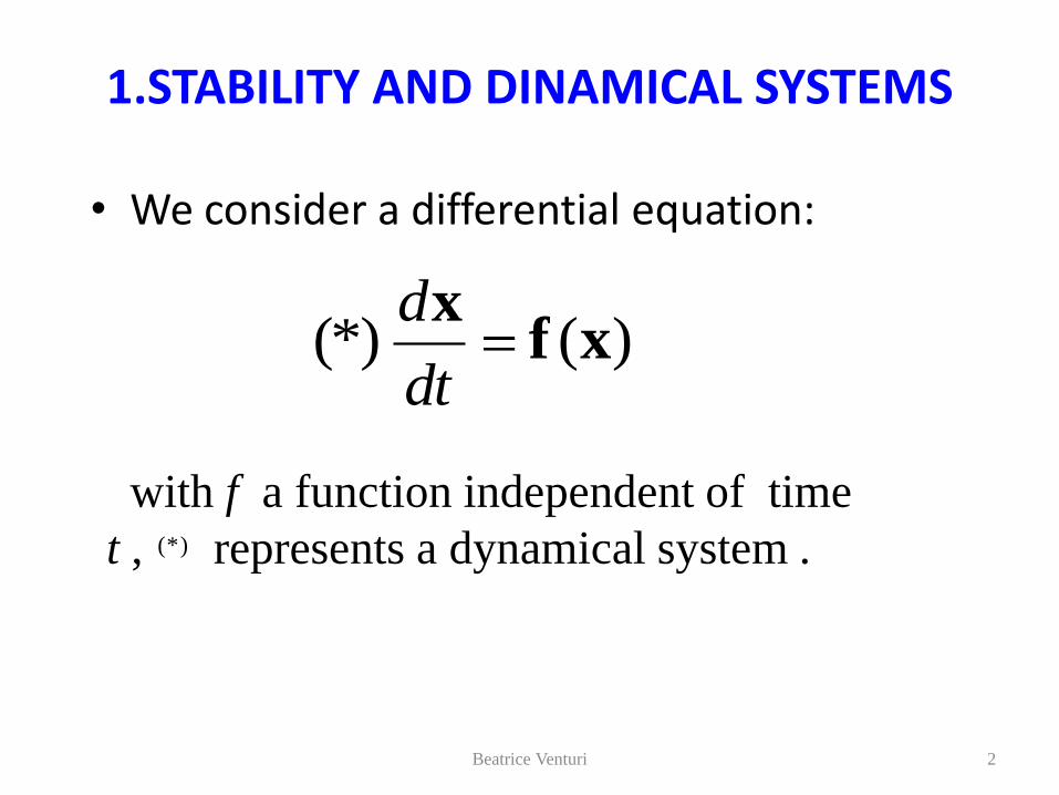
1.STABILITY AND DINAMICAL SYSTEMS
• We consider a differential equation:
Beatrice Venturi 2
)((*) xfx
dt
d
with f a function independent of time
t , represents a dynamical system . (*)

Beatrice Venturi 3
a = is an equilibrium point of our system
x(t) = a is a constant value.
such that
f(a)=0
The equilibrium points of our system are the
solutions of the equation
f(x) = 0
1.STABILITY AND DINAMICAL SYSTEMS
(*)

Market Price
Beatrice Venturi 4
)]()([ padt
dp
)()( apadt
dp
( )d s
dpa Q Q
dt
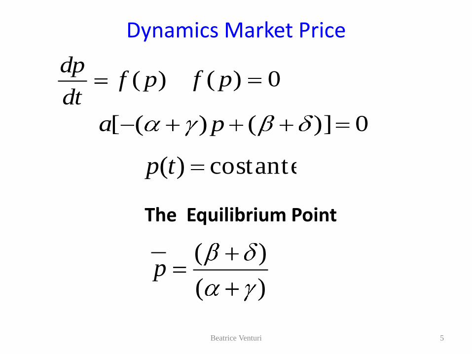
Dynamics Market Price
The Equilibrium Point
Beatrice Venturi 5
costante)(tp
)( pfdt
dp0)( pf
0)]()([ pa
)(
)(p

Dynamics Market Price
)(
,))0(()(
akdove
pepptp kt
Beatrice Venturi 6
The general solution with k>0 (k<0) converges to
(diverges from) equilibrium asintotically stable
(unstable)

The Time Path of the Market Price
Beatrice Venturi 7
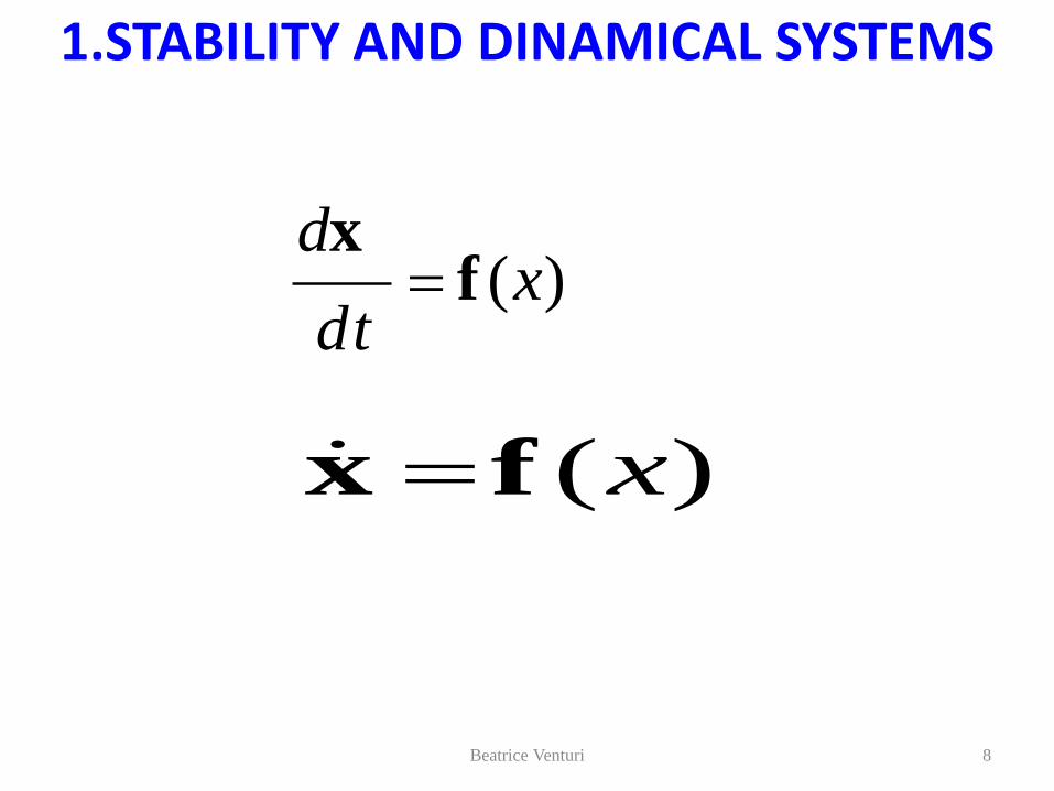
1.STABILITY AND DINAMICAL SYSTEMS
Beatrice Venturi 8
)(xdt
df
x
)(xfx
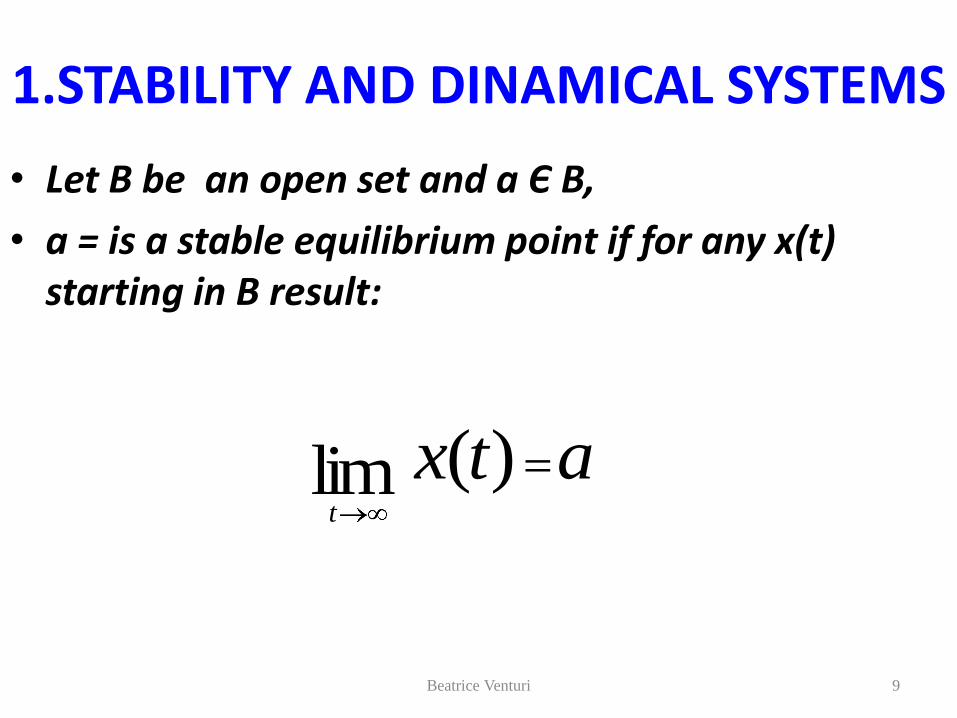
1.STABILITY AND DINAMICAL SYSTEMS
• Let B be an open set and a Є B,
• a = is a stable equilibrium point if for any x(t) starting in B result:
Beatrice Venturi 9
atxt
)(lim
A Market Model with Time
Expectation
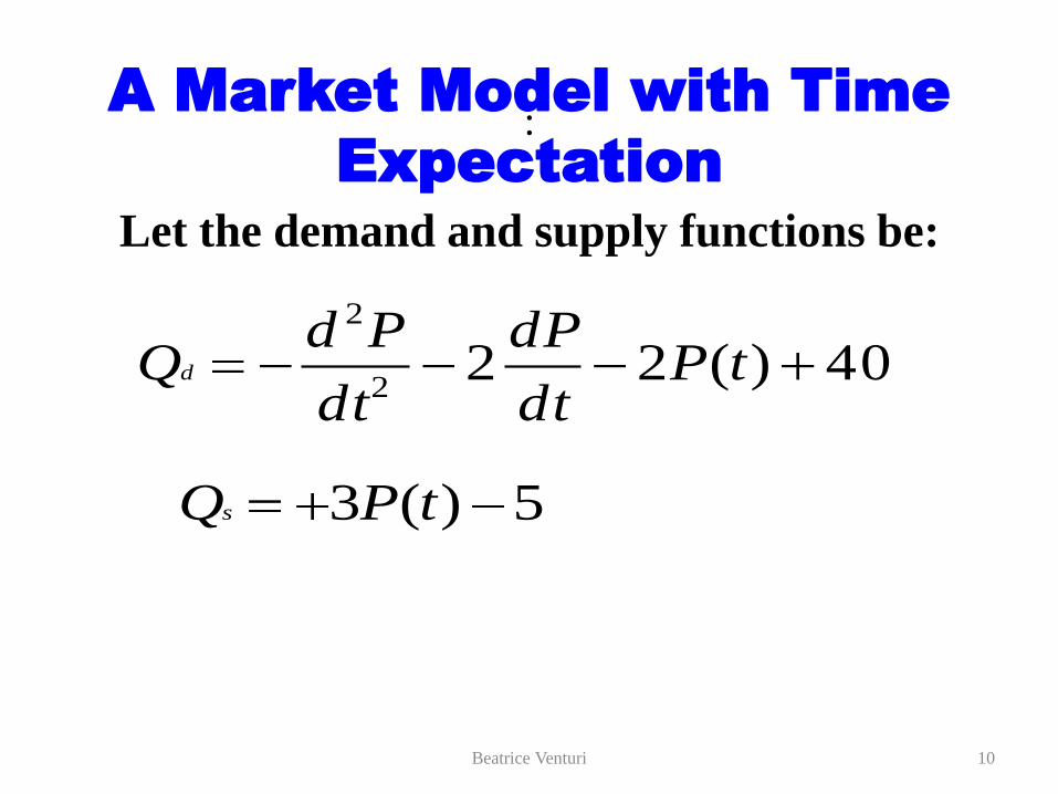
Beatrice Venturi 10
:
Let the demand and supply functions be:
40)(222
2
tPdt
dP
dt
PdQd
5)(3 tPQs

A Market Model with Time
Expectation
45)(522
2
tPdt
dP
dt
Pd
Beatrice Venturi 11
In equilibrium we have
sD QQ

A Market Model with Time
Expectation
Beatrice Venturi 12
tCetP )(
tt eCdt
PdandeC
dt
dP 2
2
2
We adopt the trial solution:
In the first we find the solution of the homogenous equation
tt eCdt
PdandeC
dt
dP 2
2
2

A Market Model with Time
Expectation
Beatrice Venturi 13
We get:
0)52( 2teC
The characteristic equation
0522
A Market Model with Time
Expectation
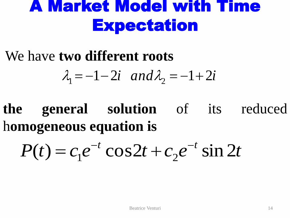
Beatrice Venturi 14
We have two different roots
iandi 2121 21
the general solution of its reduced
homogeneous equation is
tectectP tt 2sin2cos)( 21
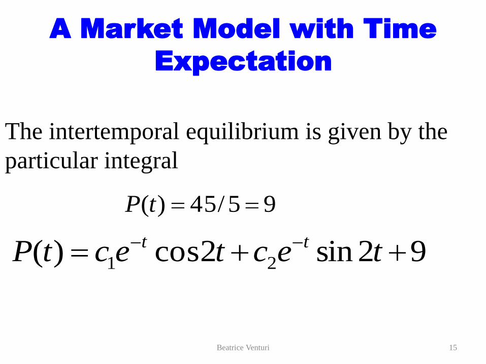
A Market Model with Time
Expectation
95/45)(tP
Beatrice Venturi 15
The intertemporal equilibrium is given by the
particular integral
92sin2cos)( 21 tectectP tt

A Market Model with Time
Expectation
• With the following initial conditions
Beatrice Venturi 16
12)0(P
1)0('P
The solution became
92sin22cos3)( tetetP tt

The equilibrium points of the system
Beatrice Venturi 17
))(),((
))(),((
)1(
2122
2111
xyxyfdx
dy
xyxyfdx
dy
STABILITY AND DINAMICAL
SYSTEMS

STABILITY AND DINAMICAL SYSTEMS
• Are the solutions :
Beatrice Venturi 18
0))(),((
0))(),(()2(
212
211
xyxyf
xyxyf

The Linear Case
Beatrice Venturi 19
)()(
)()(
(*)
tdytcxdt
dy
tbytaxdt
dx

We remember that
x'' = ax' + bcx + bdy
• by = x' − ax • x'' = (a + d)x' + (bc − ad)x
x(t) is the solution (we assume z=x)
z'' − (a + d)z' + (ad − bc)z = 0. (*)
Beatrice Venturi 20

The Characteristic Equation
If x(t), y(t) are solution of the linear system then x(t) and y(t) are solutions
of the equations (*).
The characteristic equation of (*) is
p(λ) = λ2 − (a + d)λ + (ad − bc) = 0
Beatrice Venturi 21

Knot and Focus The stable case
Beatrice Venturi 22
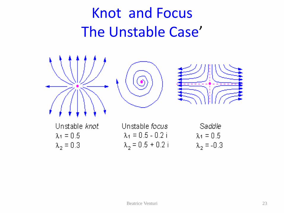
Knot and Focus The Unstable Case’
Beatrice Venturi 23

Some Examples Case a)λ1= 1 e λ2 = 3
Beatrice Venturi 24
)(2)(
)()(2
)1(
212
211
txtxdt
dx
txtxdt
dx

Case b) λ1= -3 e λ2 = -1
Beatrice Venturi 25
)(2)(
)()(2
)2(
212
211
txtxdt
dx
txtxdt
dx
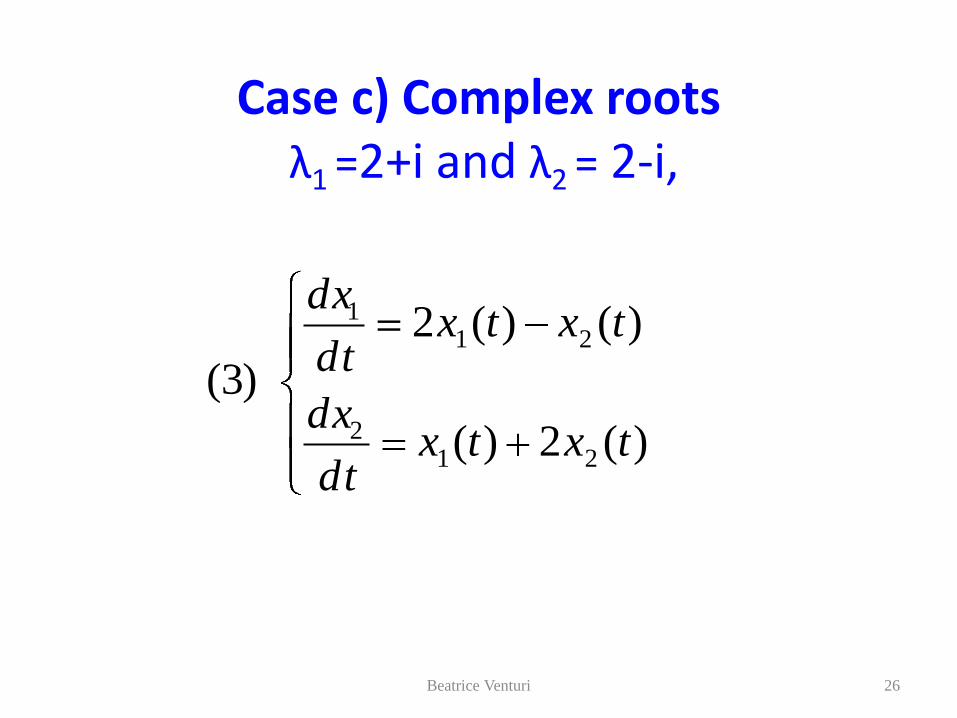
Case c) Complex roots λ1 =2+i and λ2 = 2-i,
Beatrice Venturi 26
)(2)(
)()(2
)3(
212
211
txtxdt
dx
txtxdt
dx
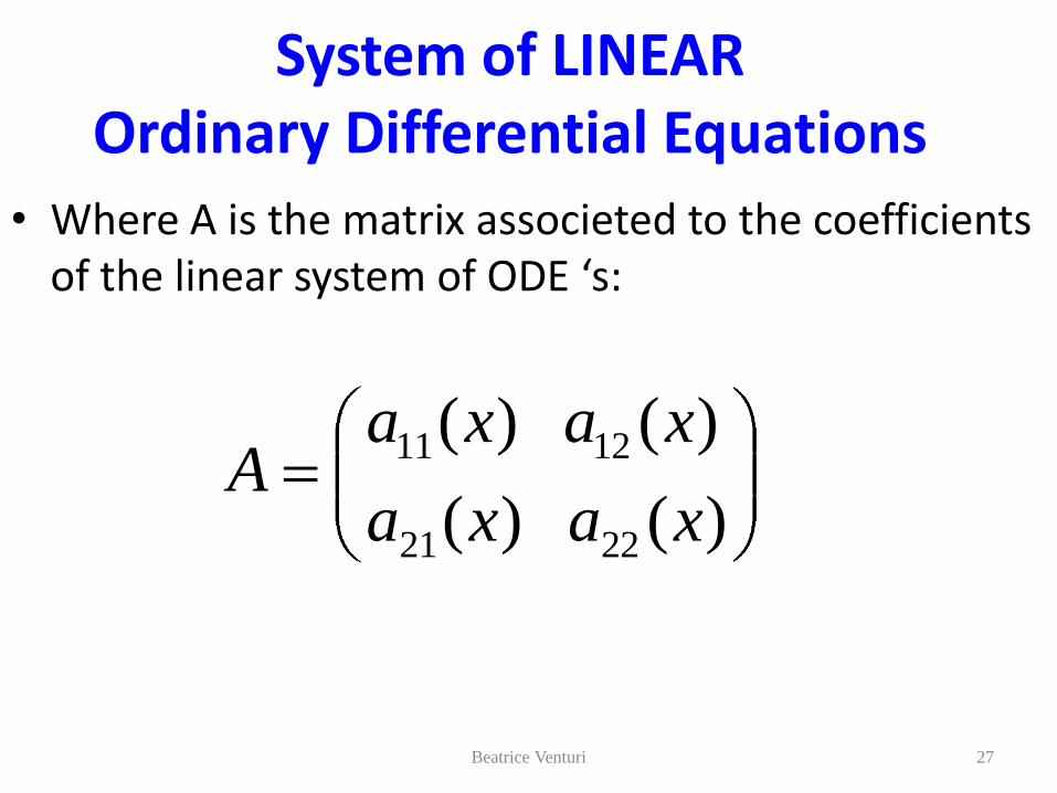
System of LINEAR Ordinary Differential Equations
• Where A is the matrix associeted to the coefficients of the linear system of ODE ‘s:
Beatrice Venturi 27
)()(
)()(
2221
1211
xaxa
xaxaA
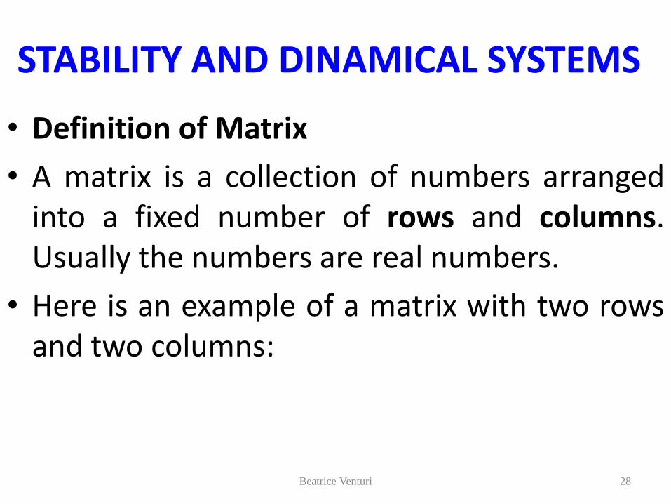
STABILITY AND DINAMICAL SYSTEMS
• Definition of Matrix
• A matrix is a collection of numbers arranged into a fixed number of rows and columns. Usually the numbers are real numbers.
• Here is an example of a matrix with two rows and two columns:
Beatrice Venturi 28
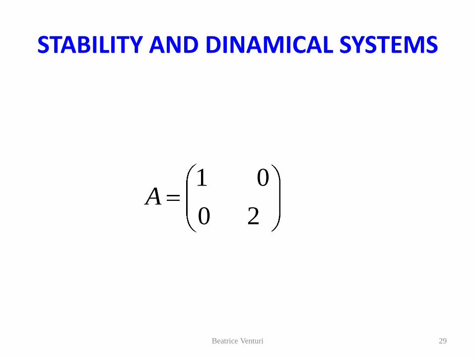
STABILITY AND DINAMICAL SYSTEMS
20
01A
Beatrice Venturi 29

STABILITY AND DINAMICAL SYSTEMS
• Examples
Beatrice Venturi 30
)(2
)(
)1(
22
11
txdt
dx
txdt
dx
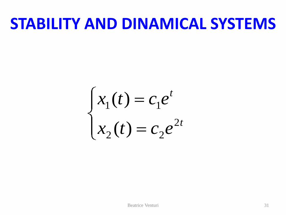
STABILITY AND DINAMICAL SYSTEMS
Beatrice Venturi 31
t
t
ectx
ectx
2
22
11
)(
)(

STABILITY AND DINAMICAL SYSTEMS
Beatrice Venturi 32
)(2
)(
)2(
22
11
txdt
dx
txdt
dx
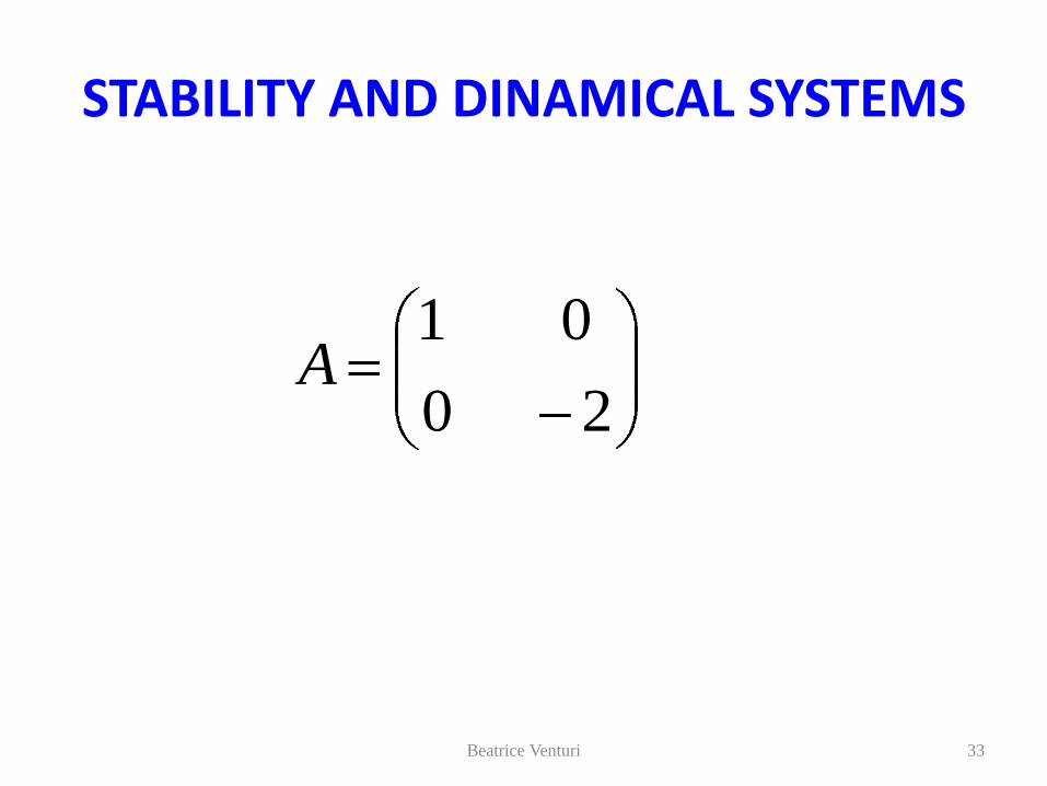
STABILITY AND DINAMICAL SYSTEMS
20
01A
Beatrice Venturi 33

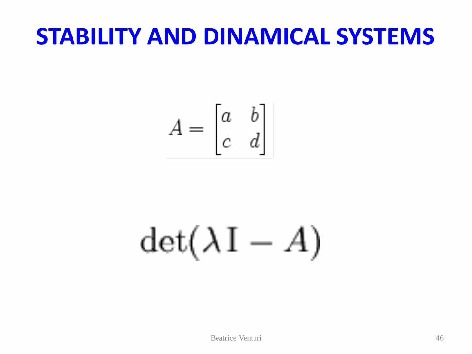
Eigenvectors and Eigenvalues of a Matrix
The eigenvectors of a square matrix are the non-zero vectors that after being multiplied by the matrix, remain parellel to the original vector.
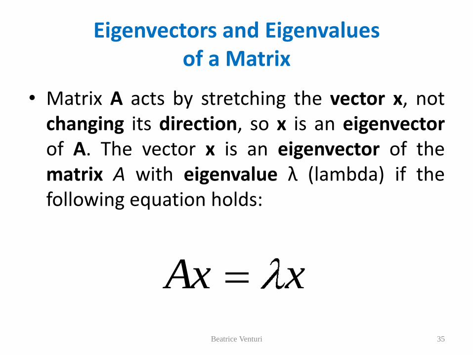
Eigenvectors and Eigenvalues of a Matrix
• Matrix A acts by stretching the vector x, not changing its direction, so x is an eigenvector of A. The vector x is an eigenvector of the matrix A with eigenvalue λ (lambda) if the following equation holds:
Beatrice Venturi 35
xAx

Eigenvectors and Eigenvalues of a Matrix
• This equation is called the eigenvalues equation.
Beatrice Venturi 36
xAx

Eigenvectors and Eigenvalues of a Matrix
• The eigenvalues of A are precisely the solutions λ to the equation:
• Here det is the determinant of matrix formed by
A - λI ( where I is the 2×2 identity matrix).
• This equation is called the characteristic equation (or, less often, the secular equation) of A. For example, if A is the following matrix (a so-called diagonal matrix):
Beatrice Venturi 37
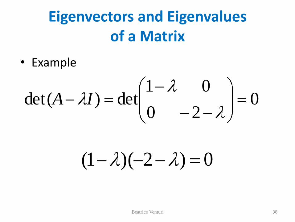
Eigenvectors and Eigenvalues of a Matrix
• Example
Beatrice Venturi 38
020
01det)det( IA
0)2)(1(

• We consider
Beatrice Venturi 39
)()()1( 212
2
xfxyadx
yda
dx
yd
STABILITY AND DINAMICAL SYSTEMS

• We get the system:
Beatrice Venturi 40
)sin(
)2(
pydt
dp
ydt
dp
STABILITY AND DINAMICAL SYSTEMS
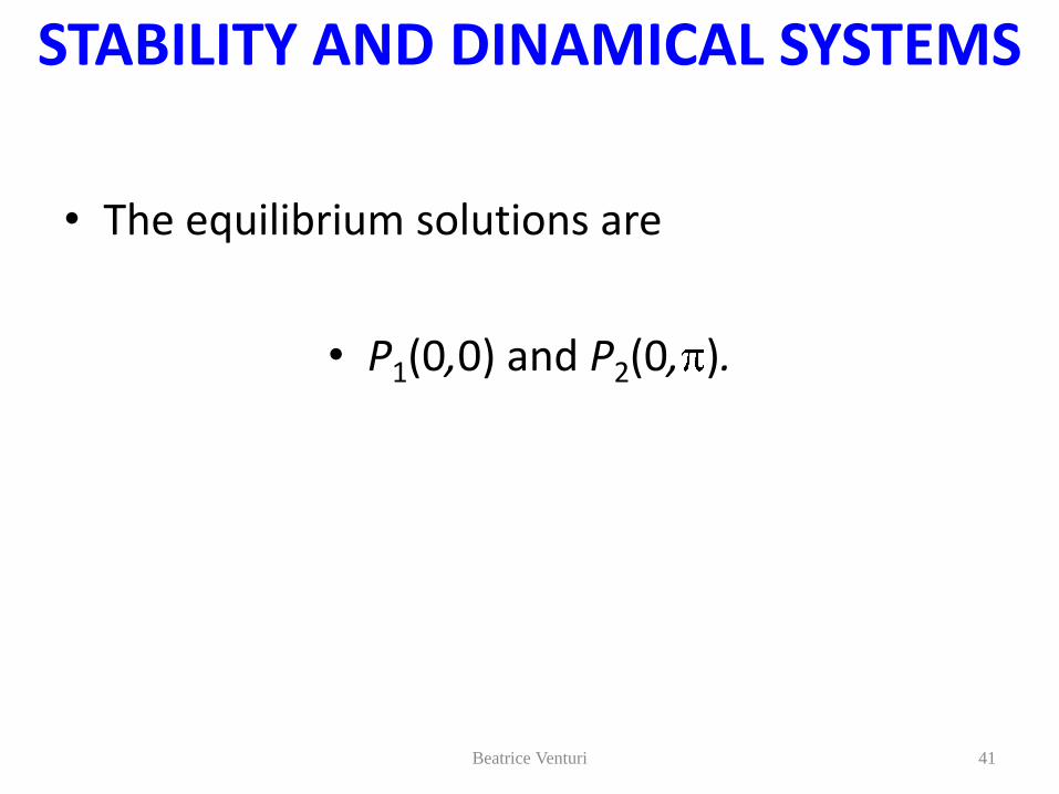
STABILITY AND DINAMICAL SYSTEMS
• The equilibrium solutions are
• P1(0,0) and P2(0, ).
Beatrice Venturi 41

STABILITY AND DINAMICAL SYSTEMS
Beatrice Venturi 42
)()(
10
12 xaxaA
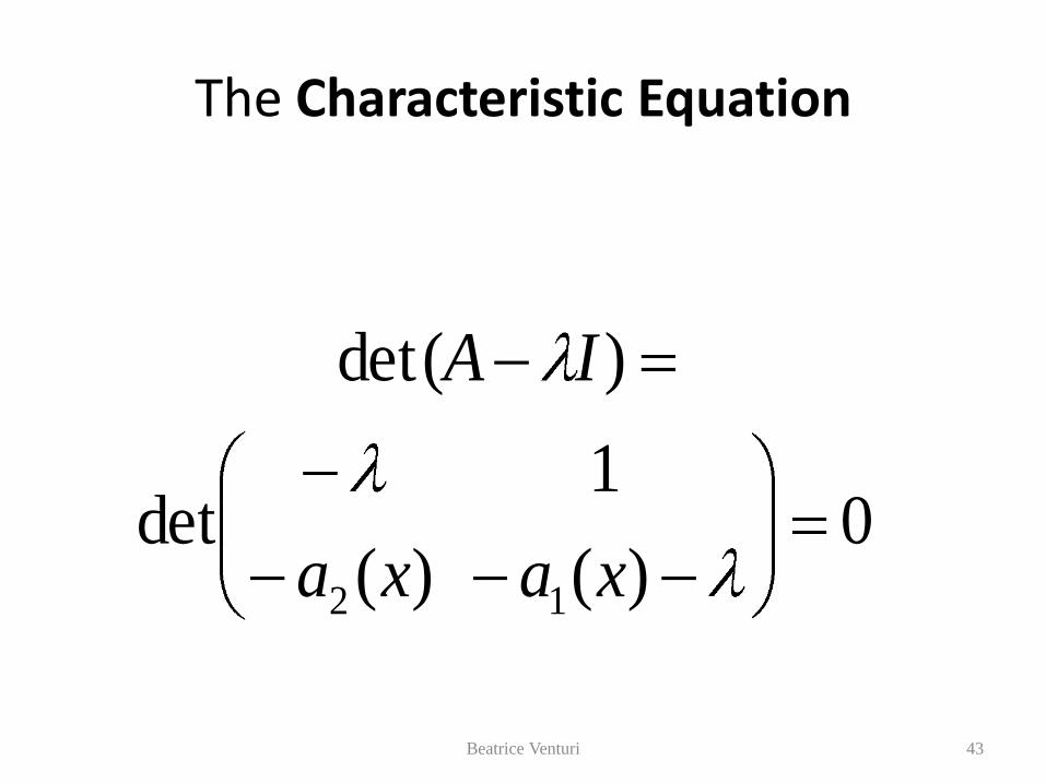
The Characteristic Equation
Beatrice Venturi 43
0)()(
1det
)det(
12 xaxa
IA
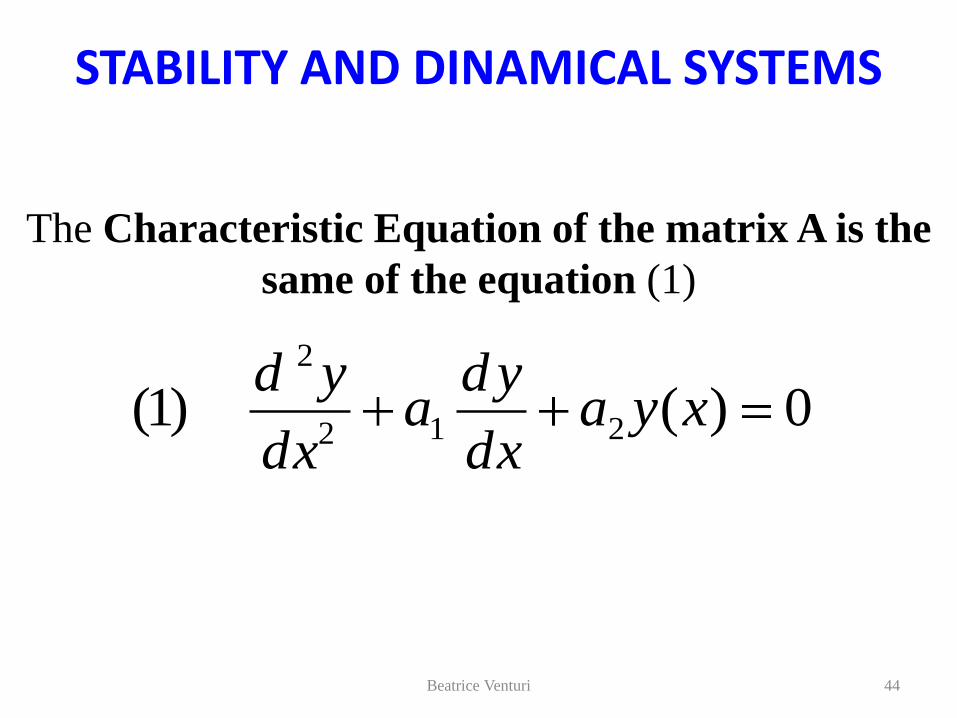
STABILITY AND DINAMICAL SYSTEMS
Beatrice Venturi 44
The Characteristic Equation of the matrix A is the
same of the equation (1)
0)()1( 212
2
xyadx
yda
dx
yd
STABILITY AND DINAMICAL SYSTEMS
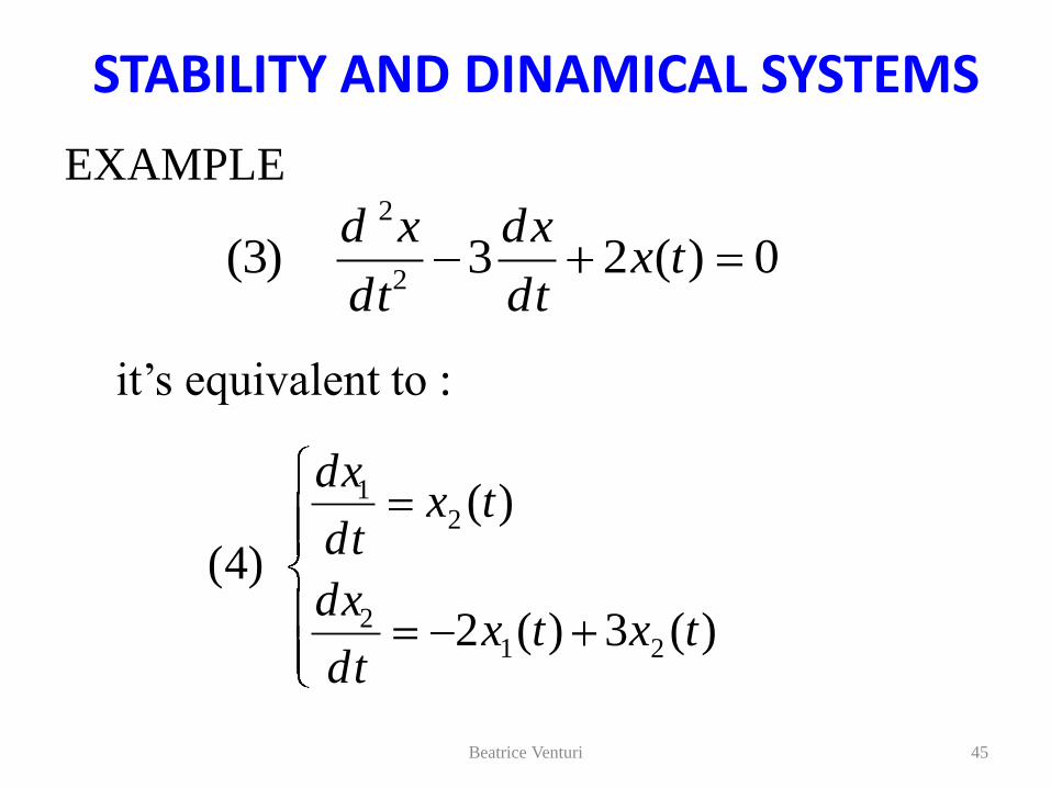
Beatrice Venturi 45
0)(23)3(2
2
txdt
xd
dt
xd
)(3)(2
)(
)4(
212
21
txtxdt
dx
txdt
dx
it’s equivalent to :
EXAMPLE
STABILITY AND DINAMICAL SYSTEMS
Beatrice Venturi 46

Eigenvalues
• p( λ) = λ2 − (a + d) λ + (ad − bc) = 0
Beatrice Venturi 47
The solutions
are the eigenvalues of the matrix A.

STABILITY AND DINAMICAL SYSTEMS
Beatrice Venturi 48
)(3
1)()(
)()(2)(
)3(
2212
2111
txtxtxdt
dx
txtxtxdt
dx

STABILITY AND DINAMICAL SYSTEMS
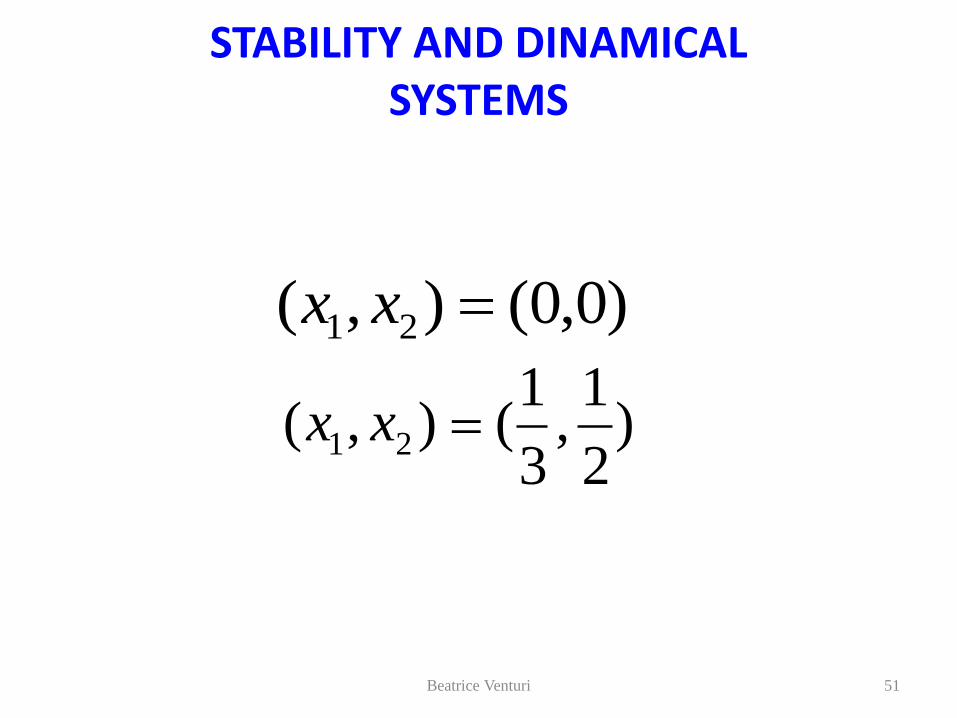
Solving this system we find the equilibrium point of the non-linear system (3):
:
Beatrice Venturi 49
0)(3
1)()(
0)()(2)(
)4(221
211
txtxtx
txtxtx
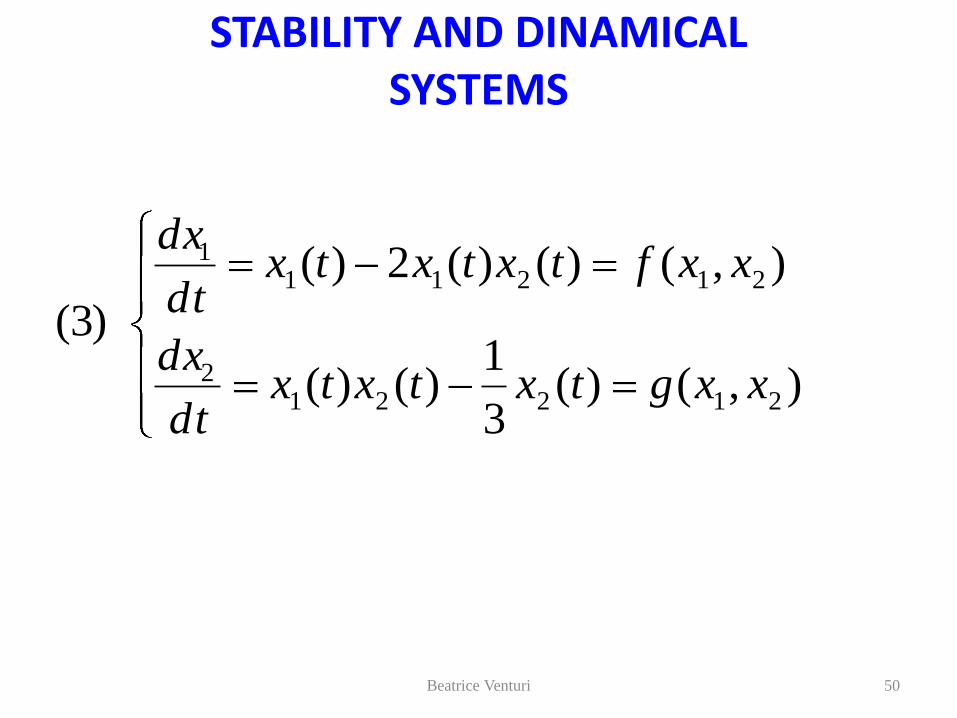
STABILITY AND DINAMICAL SYSTEMS
Beatrice Venturi 50
),()(3
1)()(
),()()(2)(
)3(
212212
212111
xxgtxtxtxdt
dx
xxftxtxtxdt
dx
STABILITY AND DINAMICAL SYSTEMS
Beatrice Venturi 51
)0,0(),( 21 xx
)2
1,
3
1(),( 21 xx

Jacobian Matrix
Beatrice Venturi 52
21
2
1
1
21 ),(
x
g
x
g
x
f
x
f
xxJ
3
1
221
),(12
12
21xx
xx
xxJ
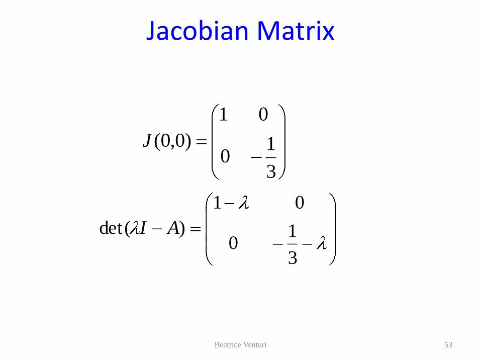
Jacobian Matrix
Beatrice Venturi 53
3
10
01
)0,0(J
3
10
01
)det( AI

Jacobian Matrix
??
??)2/1,3/1(J
Beatrice Venturi 54

Stability and Dynamical Systems
.
Beatrice Venturi 55
01
dt
dx02
dt
dx

Stability and Dynamical Systems
• Given the non linear system:
Beatrice Venturi 56
1)()(
)()(
)4(
2
2
12
211
txtxdt
dx
txtxdt
dx

Stability and Dynamical Systems
Beatrice Venturi 57
01
dt
dx
)()(
0)()(
12
21
txtx
txtx

Stability and Dynamical Systems
Beatrice Venturi 58
02
dt
dx
1)()(
01)()(
2
2
2
2
1
1
txtx
txtx

Stability and Dynamical Systems
Beatrice Venturi 59
f(x)=(x^2)-1
f(x)=x
-4.5 -4 -3.5 -3 -2.5 -2 -1.5 -1 -0.5 0.5 1 1.5 2 2.5 3 3.5 4 4.5
-4
-3
-2
-1
1
2
3
4
x
f(x)

Stability and Dynamical Systems
Beatrice Venturi 60
f(x)=e^x
f(x)=e^(-2x)
-4.5 -4 -3.5 -3 -2.5 -2 -1.5 -1 -0.5 0.5 1 1.5 2 2.5 3 3.5 4 4.5
-4
-3
-2
-1
1
2
3
4
x
f(x)
61
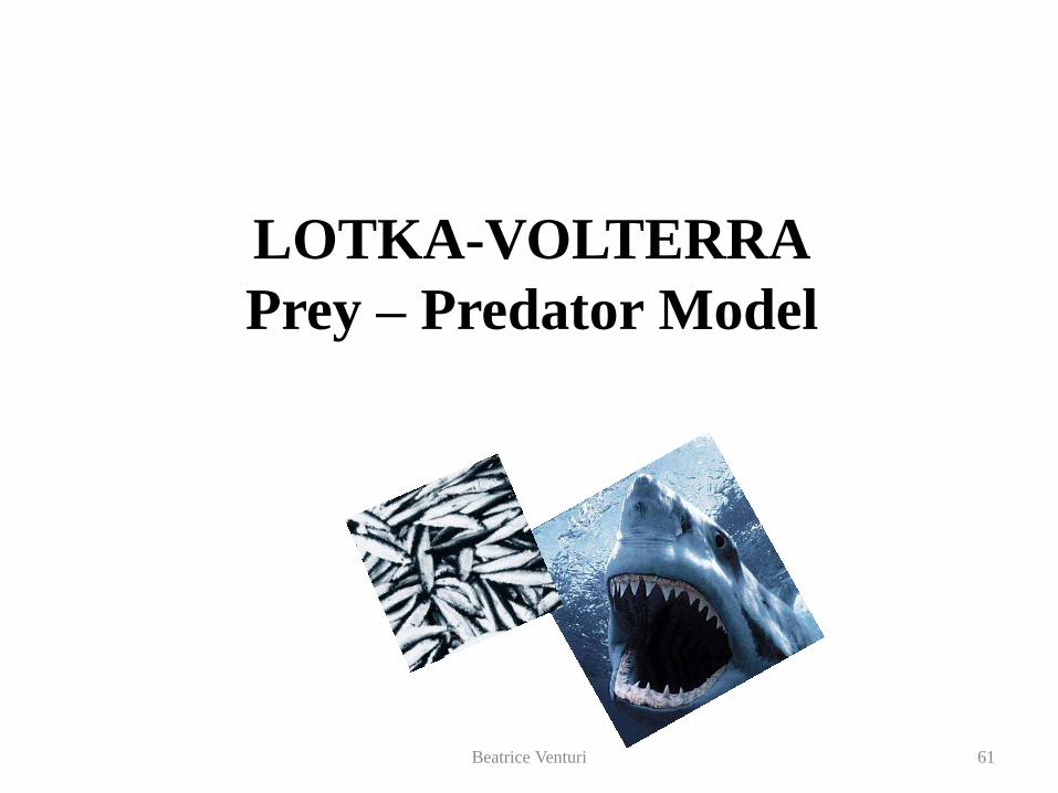
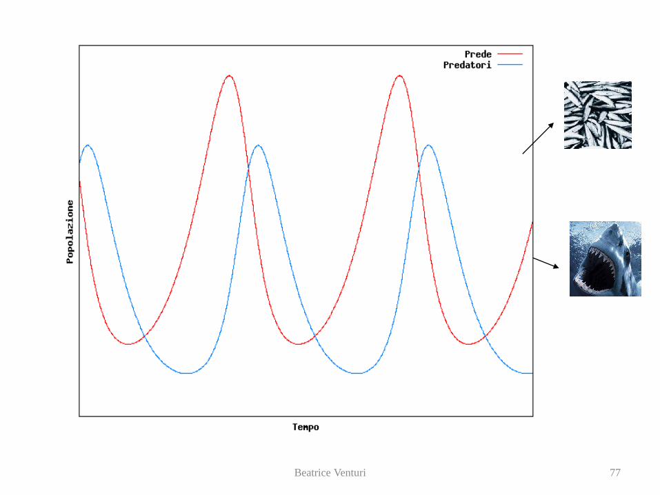
LOTKA-VOLTERRA
Prey – Predator Model
Beatrice Venturi

The Lotka-Volterra Equations,

63
We shall consider an ecologic system
PREy PREDATOR
Beatrice Venturi

Predator-Prey cycles
1
1
dFa b S
F dtdS
c d FS dt
Rate of growth of Fish
Food supply Interactions with Sharks
Rate of growth of Sharks
Rate of death in absence of Fish to eat
Interactions with Fish
• Generates a cycle: – Lots of fish—>lots of interactions with Sharks—>rapid growth of Sharks—>Fall in Fish numbers—>less interactions with Sharks —>Fall in Shark numbers—>Lots of fish again...
dFa F b S F
dtdS
c S d F Sdt
Linear bits unstable
near equilibrium
Nonlinear bits stabilise far from
equilibrium

Beatrice Venturi 65
),()()()(
),()()()(
(*)
SFgtStdFtcSdt
dS
SFftStbFtaFdt
dF
The Model
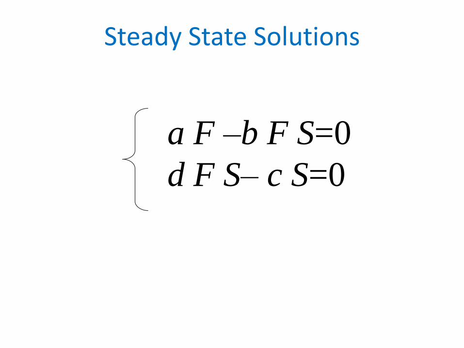
Steady State Solutions
a F –b F S=0
d F S– c S=0

The Jacobian Matrix
J =
∂f/∂F ∂f/∂S
∂g/∂F ∂g/∂S

Eigenvalues
p( λ) = λ2 − Tr J λ + det J = 0
Beatrice Venturi 68
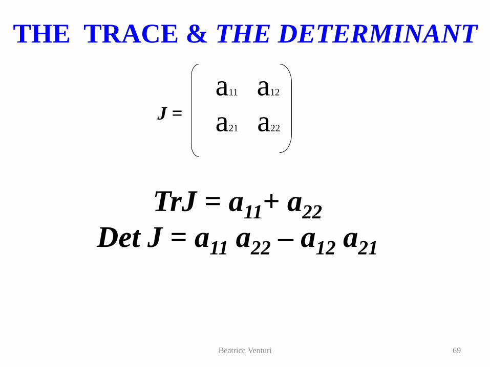
69
TrJ = a11+ a22
Det J = a11 a22 – a12 a21
a11 a12
a21 a22 J =
THE TRACE & THE DETERMINANT
Beatrice Venturi
70
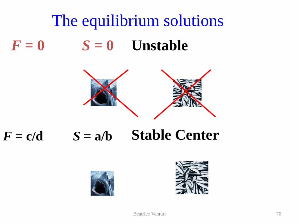
The equilibrium solutions
F = 0 S = 0 Unstable
F = c/d S = a/b Stable Center
Beatrice Venturi
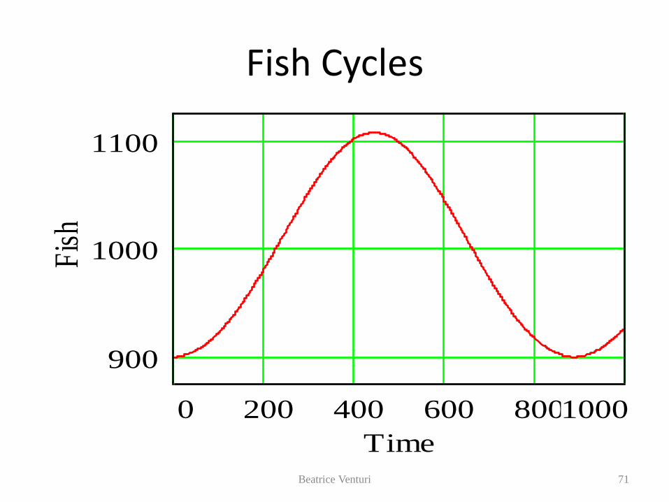
Fish Cycles
Beatrice Venturi 71
0 200 400 600 8001000
900
1000
1100
Time
Fis
h
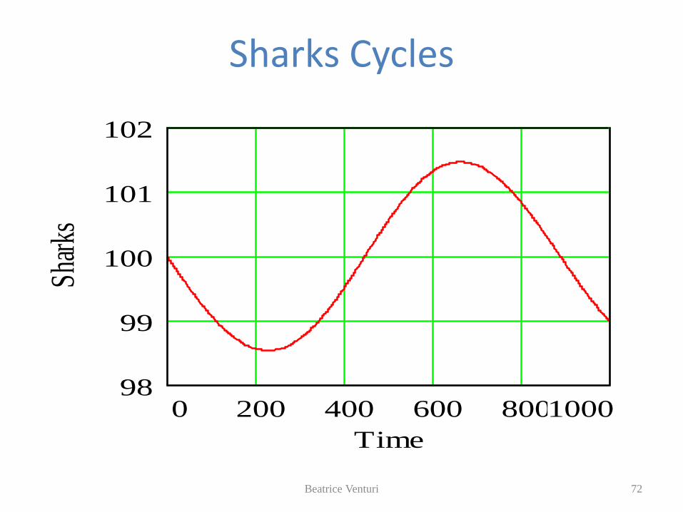
Sharks Cycles
Beatrice Venturi 72
0 200 400 600 800100098
99
100
101
102
Time
Shar
ks
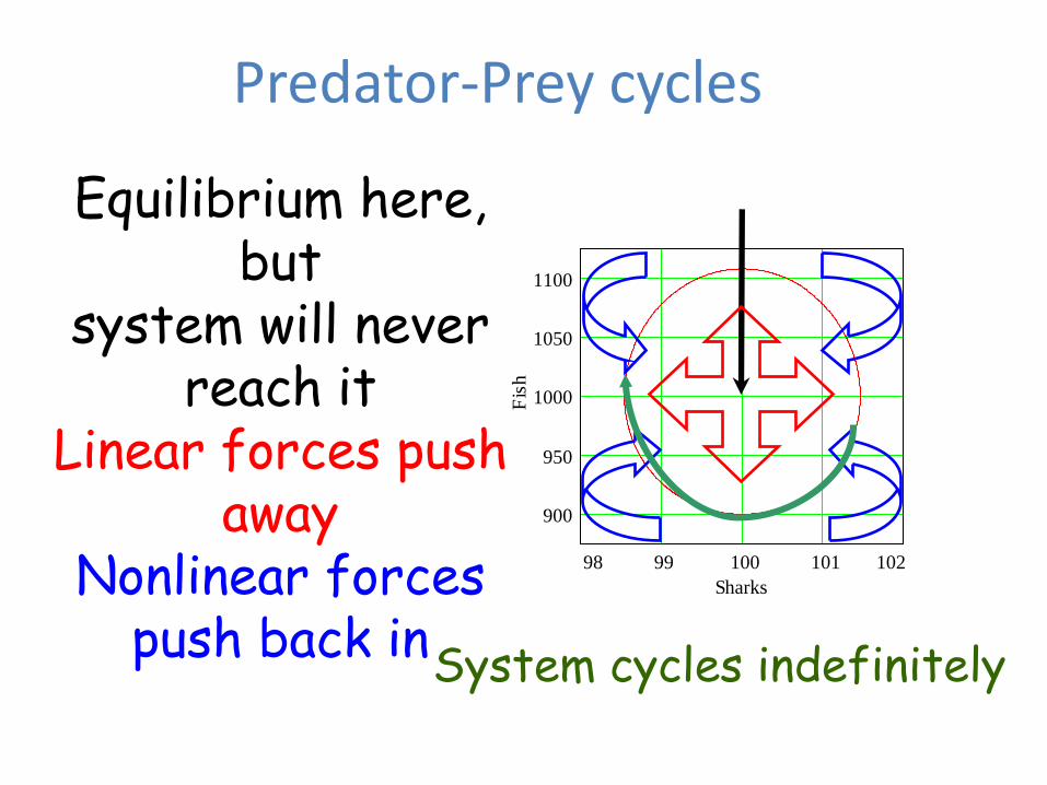
Predator-Prey cycles
98 99 100 101 102
900
950
1000
1050
1100
Sharks
Fis
h
Equilibrium here, but
system will never reach it
Linear forces push away
Nonlinear forces push back in
System cycles indefinitely
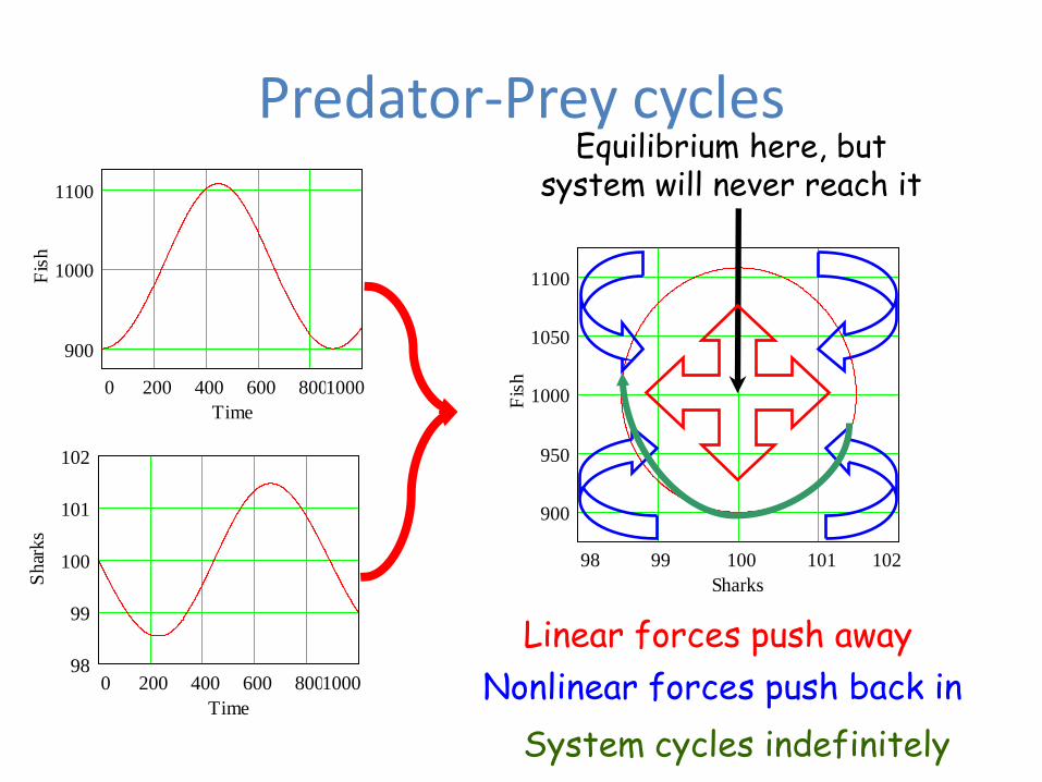
Predator-Prey cycles
0 200 400 600 8001000
900
1000
1100
Time
Fis
h
0 200 400 600 800100098
99
100
101
102
Time
Shar
ks
98 99 100 101 102
900
950
1000
1050
1100
Sharks
Fis
h
Equilibrium here, but system will never reach it
Linear forces push away
Nonlinear forces push back in
System cycles indefinitely
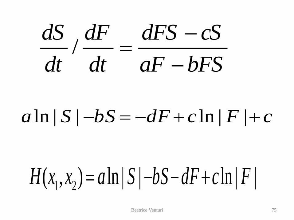
75
bFSaF
cSdFS
dt
dF
dt
dS/
cFcdFbSSa ||ln||ln
||ln||ln),( 21 FcdFbSSaxxHBeatrice Venturi
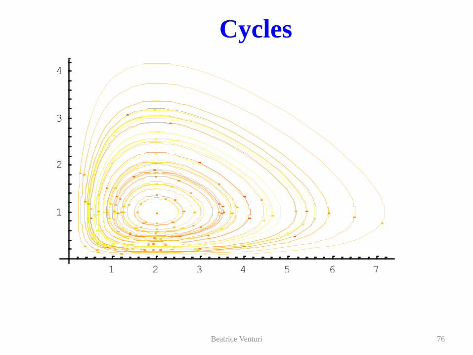
76
1 2 3 4 5 6 7
1
2
3
4
Cycles
Beatrice Venturi
77 Beatrice Venturi