stability analysis of linear multistep methods for classical elastodynamics

Comput. Methods Appl. Mech. Engrg. 193 (2004) 2169–2189

www.elsevier.com/locate/cma

Stability analysis of linear multistep methodsfor classical elastodynamics

Ignacio Romero *

Departamento de Mecanica de Medios Continuos y Teorıa de Estructuras, E.T.S. Ingenieros de Caminos,

C/Profesor Aranguren s/n, Ciudad Universitaria, 28040 Madrid, Spain

Received 8 August 2002; received in revised form 13 May 2003; accepted 2 January 2004

Abstract

We propose an analysis of the stability of linear multistep methods when they are employed for the numerical

integration in time of the equations resulting from the finite element spatial discretization of the problem of linear

elastodynamics. First, the notion of stability is defined for the global equations of the space–time discrete problem.

Second, a spectral analysis is employed to identify simpler modal criteria that are necessary and sufficient for stability.

These new criteria are stronger than the classical spectral stability criterion which, furthermore, is shown not to be

sufficient for global energy stability. The results of the analysis are applied to the study of several widely employed

linear multistep integrators.

2004 Elsevier B.V. All rights reserved.

Keywords: Linear elastodynamics; Stability; Modal analysis; Finite elements; Linear multistep methods

1. Introduction

Semidiscretization techniques are widely employed for the numerical approximation of the equations ofelastodynamics. They consist of two successive steps: a spatial discretization of the partial differential

equations that govern the problem––by finite elements or a similar method––and the numerical integration

in time of the ordinary differential equations resulting from the first step. The solution to the spatial

projection is called the semidiscrete approximation, and when the latter is numerically integrated in time,

results in the fully discrete solution.

In solid and structural engineering, the most commonly used time integrators can be formulated as linear

multistep methods for the second order differential equations of elastodynamics [10]. These general class of

algorithms include, among others, Newmarks method [19], Houbolts method [15], Parks method [20],Wilsons h-method [24], the HHT method [14], Hulberts a-method [5], Bazzis q-method [3], etc. See, e.g.,

* Tel.: +91-336-5394; fax: 91-336-6702.

E-mail address: [email protected] (I. Romero).

0045-7825/$ - see front matter 2004 Elsevier B.V. All rights reserved.

doi:10.1016/j.cma.2004.01.012

mail to: [email protected]

2170 I. Romero / Comput. Methods Appl. Mech. Engrg. 193 (2004) 2169–2189

[4,16,17] for a review of many of them and the semidiscretization approach to the solution of linear elasto-dynamics.

The convergence of this type of space–time discretizations depends on the convergence of both the

spatial and time approximations. The convergence of the first approximation has been addressed, for

example, in [1,11,23, p. 254]. On the other hand, the convergence of the time integration phase has been

extensively studied in the engineering literature, mostly making use of spectral techniques which simplify

the analysis and provide systematic ways to asses the performance of specific time stepping schemes, such as

the ones mentioned in the previous paragraph. Among the most useful results provided by this type of

analysis is the so-called spectral stability criterion. This condition, which will be referred hereafter as theclassical spectral stability criterion, determines the stability of a linear multistep method applied to the

equations of elastodynamics by examining only the eigenvalues of the corresponding modal amplification

matrices. Other full convergence analysis of finite elements in space and linear multistep methods in time for

second order hyperbolic equations can be found in [7,9]. The approach followed in the convergence analysis

of these last articles is different from the one described above: instead of using the semidiscrete solution as a

intermediate step between the exact and fully discrete solutions, a different energy projection of the exact

solution is employed which simplifies the analysis.

In [22], we presented an analysis of the convergence of the space–time discretization of the equations ofelastodynamics, when the spatial approximation is done with finite elements and the time integration with

one-step methods. After reexamination of the global and modal conditions for stability and convergence of

the time integration scheme, sufficient conditions for global and modal energy stability of the integrators

considered were identified. Remarkably, the modal stability criteria found were more stringent than the

classical spectral stability condition. When applied to the analysis of Newmarks method, we concluded that

some members of the family which are stable according to the classical spectral stability criterion are not

globally (energy) stable when both the mesh and time step sizes go to zero.

In this article we extend some of the results of [22], proposing a stability analysis in the energy norm of amore general class of linear multistep methods, which include the time stepping schemes most commonly

employed in solid and structural elastodynamics. As in [22], the starting point is the study of the global

equations of the method and in this context an appropriate notion of energy stability is defined. Two

aspects are important for this stability analysis: first, the multistep methods have to be formulated only in

terms of the displacements and velocities, avoiding the presence of acceleration variables or higher order

rates; second, the constants appearing throughout the analysis cannot depend on the number of equations

of the semidiscrete problem. This last condition, which can be ignored when analyzing the integration of

any single system of ordinary differential equations, must be taken into account in the problem of interestsince we are ultimately interested in proving that the total error goes to zero when the number of equations

in the discrete model goes to infinity (and the time step size goes to zero).

Once the general stability concept is stated, our analysis employs the modal decomposition of the

algorithmic equations to obtain simpler conditions which are necessary and sufficient for the stability of the

time integration of the global problem. The analysis presented reveals that the stability bounds obtained

with the spectral analysis of the algorithms must be uniform (i.e. do not depend on the modal frequency or

the number of modes) or otherwise they will not guarantee the convergence of the global solution under

arbitrary loading and initial conditions. In essence, this statement is equivalent to the fact that the stabilitybounds in the global solution cannot depend on the mesh size of the spatial discretization, as discussed

above. The main practical consequence of this fundamental result is that the modal stability criteria pro-

posed are stronger that the classical spectral stability criterion, which does not imply the uniformity of the

stability bounds. For this reason, it is shown that the classical spectral stability criterion is a necessary but

insufficient condition for energy stability of the time integration phase.

The results obtained in the stability analysis are employed for the study of three commonly used mul-

tistep time integration algorithms: the HHT method, Houbolts method, and Parks method. Remarkably,

I. Romero / Comput. Methods Appl. Mech. Engrg. 193 (2004) 2169–2189 2171

the stability conditions identified throughout the analysis can only guarantee the unconditional energystability of the last of these methods, in contrast with what is usually accepted.

An outline of the rest of the article is as follows. In Section 2 the equations of linear elastodynamics are

summarized and the space–time discretization procedure is reviewed. In Section 3 the main notion of energy

stability for linear multistep methods is defined. The modal stability analysis of the time integration

algorithms is addressed in Section 4, where modal stability conditions are identified which are necessary and

sufficient for energy stability. The results obtained are employed in Section 5 to study the stability of three

commonly used time integration schemes. Section 6 closes the article, summarizing the main results and

conclusions obtained.

2. The spatial and time discretization of the equations of linear elastodynamics

A review of the equations of linear elastodynamics is presented in this section and their full space–time

discretization is summarized. The discretizations discussed are based on finite elements in space and linear

multistep integrators in time and the analysis of this particular combination of numerical techniques will be

addressed in Section 3. The notation employed in this section follows closely [22] and we refer to this workand references therein for more details on the theory and discretization of the problem of interest.

2.1. The weak form of the equations of linear elastodynamics

First, the initial boundary value problem of linear elastodynamics is presented in weak form, since the

numerical methods considered in this work are based directly on this variational statement of the equations.

For this, consider a domain X in Rndim , where ndim can be 2 or 3, and points inside it labeled by x with

displacement function uðx; tÞ 2 Rndim at time t. The set X represents the space occupied by an elastic body,assumed homogeneous and isotropic, of density q and elasticity tensor C. Let C be the boundary of X and nthe unit vector normal to C in the outward direction. The boundary consists of two disjoint parts Cu and Ct

such that C ¼ Cu [ Ct. The displacement of points on the boundary Cu is zero and the tractions are known

to have value t on Ct. The dynamical problem is studied on the time interval I ¼ ½0; T .In order to formulate the variational equations, define the set of trial functions

S ¼ fu : XI ! Rndim ; uð; tÞ 2 ½H 1ðXÞndim ; _uðx; Þ; €uðx; Þ 2 ½L2ðXÞndim ; u ¼ 0 on Cu Ig; ð2:1Þand the set of weighting functions

V ¼ fw : X ! Rndim ; w 2 ½H1ðXÞndim ; w ¼ 0 on Cug: ð2:2ÞGiven some known external body force b, the weak solution of the equations of elastodynamics is the

displacement function uðx; tÞ in the trial space S that verifiesZXr e½wdXþ

ZXq _v wdX ¼

ZXb wdXþ

ZCt

t wdC; v ¼ _u ð2:3Þ

with r ¼ rT, for all weighting functions w in V. Also, the solution u must satisfy the following initial

conditions:

uðx; 0Þ ¼ u0ðxÞ; _uðx; 0Þ ¼ v0ðxÞ; x 2 X; ð2:4Þwhere u0, v0 are the known initial displacement and velocity, respectively. The strain operator e and the

stress tensor r are defined respectively as

e½u ¼ 1

2ðruþ ðruÞTÞ; rðeÞ ¼ Ce: ð2:5Þ


We have employed the notation ðÞ_ ¼ oðÞot for the time derivative. The dot product in (2.3) and hereafter

denotes the inner product between tensors of any order resulting from the contraction of all their indices.

A pair ðuðx; tÞ; vðx; tÞÞ will be referred to as a configuration and will be denoted by the symbol U. Given

any configuration U, its energy EðUÞ is defined as the sum of kinetic and potential energy of a body with

displacement uðx; tÞ and velocity vðx; tÞ, i.e.,

EðUÞ ¼ZX

1

2e½uðx; tÞ Ce½uðx; tÞdXþ

ZX

1

2qvðx; tÞ vðx; tÞdX: ð2:6Þ

Using the concept of energy, the energy norm of a configuration is defined as

kUkE ¼ffiffiffiffiffiffiffiffiffiffiffiEðUÞ

p: ð2:7Þ

The properties of the potential and kinetic energy guarantee that the function k kE has indeed all the

properties of a norm. Moreover, it is a natural norm for the problem (2.3) which is reasonable for studying

the convergence and stability of solutions.

2.2. The spatial discretization

The variational problem (2.3) is discretized in space using finite elements. For this, define a mesh on Xconsisting on nel elements, connected at nnode nodes. The mesh is assumed to be regular and let h denote the

mesh size parameter. In the Galerkin method, the trial space S and the weighting space V are replaced in

the weak form by corresponding finite dimensional subsets of the form

Sh ¼ uhðx; tÞ(

¼Xnnodea¼1

NaðxÞuaðtÞ with uaðtÞ 2 ½C2ðIÞndim ; uhðx; tÞ ¼ 0 on Cu

);

Vh ¼ whðxÞ(

¼Xnnodea¼1

NaðxÞwa; with wa 2 Rndim ; whðxÞ ¼ 0 on Cu

);

ð2:8Þ

where C2ðIÞ is the space of continuous functions in I, with continuous derivatives up to order 2. Theshape functions Na : X ! R are piecewise polynomials with compact support and sufficient smoothness

properties. The vectors uaðtÞ are the nodal displacement functions and likewise, wa are the nodal values of

the variations. The semidiscrete solution uhðx; tÞ is the displacement function in Sh that verifies (2.3) for

every whðxÞ in the space Vh. Denoting by ndof the number of unknown nodal components of the dis-

placement uh, the weak equation (2.3) can be written, after a standard manipulation, in matrix form as

system of ndof ordinary differential equations:

M€UðtÞ þKUðtÞ ¼ fðtÞ; t 2 I;

Uð0Þ ¼ U0;

_Uð0Þ ¼ V0:

ð2:9Þ

where M is the mass matrix, K the stiffness matrix, f the vector of external forces and U the vector of nodal

displacements, which collects in a single vector all the unknown nodal components ua. The solution to the

system of ordinary differential equations (2.9) is denoted Uh ¼ ðuh; vhÞ with vhðx; tÞ ¼ _uðx; tÞ. By abuse ofnotation, the same symbol will sometimes refer to the vector form of the semidiscrete displacement and

velocity, i.e., Uh ¼ ðU; _UÞ.

2.3. The time discretization

To complete the numerical approximation of the equations of motion, the system of ordinary differential

equations (2.9) needs to be solved and a numerical method is used to integrate it. In this work we consider a


certain type of linear multistep algorithms which includes the most commonly employed integrators forlinear elastodynamics, namely Newmarks method, the HHT method, the Wilsons h-method, Hulberts a-method, and other. Before defining this class of methods, consider a partition of the time interval I into Nclosed subintervals ½tn; tnþ1 of constant size Dt ¼ tnþ1 tn, where 0 ¼ t0 < t1 < < tN1 < tN ¼ T and de-

note by yn the numerical approximation at time tn of a variable y. With this notation, we have the following:

Definition 2.1. ([10]) A linear k-step method for the second order differential equation (2.9) is a rule of the

formXki¼0

½aiMUnþi þ Dt2biðKUnþi þ fðtnþiÞÞ ¼ 0; ð2:10Þ

together with the initial conditions

Ui ¼ UðiDtÞ; i ¼ 1 k; . . . ; 0: ð2:11ÞThe scalars ai; bi are constants and define each method.

The initial conditions (2.11) are given at negative time instants for simplicity of notation and to simplify

the proofs of the analysis in Section 3 but are equivalent to the usual initial conditions at positive time

instants, up to a time shift.As noted above, the most commonly used integration schemes in elastodynamics are linear multistep

methods for the second order equation (2.9) and therefore may be formulated as in equation (2.10).

However, the standard way of presenting these time-marching algorithms is not the one described in the

previous definition but rather employing a velocity approximation Vn and an acceleration approximation

An. After eliminating these two fields from the equations (by expressing them in terms of the displacements

Un at different time instants) the form (2.10) is recovered.

For the analysis presented in Section 3 it proves convenient to use yet a different but equivalent

description of linear multistep methods. This third formulation can be obtained from the standard for-mulation of the integrators by eliminating the acceleration field, or any other high order rate, and leaving

the recursive equations of the method in terms of the displacement and velocity vectors. In this way only the

configuration approximations Uhn ¼ ðUn;VnÞ appear in the formulation and we have the following alter-

native definition of a linear multistep method:

Definition 2.2. Let Uhn denote the algorithmic approximation to UhðtnÞ, the solution of the system of dif-

ferential equations (2.9). The k-step methods of Definition 2.1 are those in which the approximate solution

Uhnþk can be obtained from the solutions at previous steps with the recursive formulaXk

i¼0

LhiU

hnþi þ Dtgh

nþi ¼ 0; ð2:12Þ

together with the initial conditions

Uhi ¼ UhðiDtÞ; i ¼ 1 k; . . . ; 0: ð2:13Þ

The matrices Lhi are constant, have dimension 2ndof 2ndof and can be partitioned into four square blocks

of dimension ndof , each of these depending linearly on the mass, stiffness and identity matrices. Similarly,

ghnþi are vectors of size 2ndof which can be partitioned into two vectors of size ndof and consisting on the

force vector fðtnþiÞ possibly multiplied by a scalar, the mass matrix or the stiffness matrix.

In the following section we will consider integration schemes of the form (2.12) for the semidiscrete

equations of elastodynamics (2.9).


Remark 2.3

ii(i) The choice of initial conditions (2.11) and (2.13) is useful for the analysis but it is not the only one

possible. There are other ways to provide initial conditions for a multistep method such as using a

one step method or a Runge–Kutta method. We refer to standard books on the topic (e.g.

[8,13,18]) for details.

i(ii) Since Eq. (2.12) is used to solve for the configuration Uhnþk the square matrix Lh

k must be invertible.

(iii) The particular form of Eqs. (2.12) is key for the analysis. Since we will be interested in obtaining errors

in the energy norm, the acceleration field must be eliminated from the formulation while the velocityfield must remain.

Example 2.4. To show two of the possible formulations of a linear multistep method, consider for example

the HHT method [14]. This widely used method is usually formulated in terms of three fields: the dis-

placement vector Un, the velocity vector Vn and the acceleration vector An. The equations that define this

algorithm are

MAnþ1 þKUnþa ¼ fnþa;

Unþ1 ¼ Un þ DtVn þDt2

2½ð1 2bÞAn þ 2bAnþ1;

Vnþ1 ¼ Vn þ Dt½ð1 cÞAn þ cAnþ1:

ð2:14Þ

In these equations, and for the rest of the article, the notation ðÞnþa denotes the convex combination

ð1 aÞðÞn þ aðÞnþ1, for any scalar 06 a6 1. The scalars a;b; c that determine each of the members of the

HHT family must satisfy

0:76 a6 1; b ¼ 1

a2

2; c ¼ 3

2 a: ð2:15Þ

If the acceleration is eliminated from Eqs. (2.14), the HHT method can be written in the form (2.12) to-

gether with the definitions

Lh2 ¼

1þ abDt2M1K 0

acDtM1K 1

" #;

Lh1 ¼

a2þ b 2ab

Dt2M1K 1 Dt1

ðaþ c 2acÞDtM1K 1

264

375;

Lh0 ¼

ð1 aÞ 1

2 b

Dt2M1K 0

ð1 aÞð1 cÞDtM1K 0

264

375;

ghnþ2 ¼

abDtM1fnþ2;

acM1fnþ2

( );

ghnþ1 ¼

2ab a2 b

DtM1fnþ1

ð2ac a cÞM1fnþ1

8<:

9=;;

ghn ¼

ð1 aÞ b 1

2

DtM1fn

ð1 aÞðc 1ÞM1fn

8<:

9=;;

ð2:16Þ


By further eliminating the velocity field, one arrives, after a lengthy but straightforward manipulation, to

the linear multistep form (2.10) of the HHT method in terms of the displacement vector Un at different time

instants. This last form of the method will not be used in the analysis hence we do not present it here.

3. Stability of fully discrete solutions

The space–time discretization described in Section 2 can only be useful in practice if it can be shown thatthe fully discrete solution Uh

n converges to the exact solution U at time tn as the mesh parameter h and the

time step size Dt tend to zero. In the same spirit of [22], we define precise notions of convergence of the

space–time discretization and focus on the definition and verification of the stability in the time integration.

The convergence and stability notions proposed are based on the energy norm (2.7). In this particular

norm, we define the total error of the discretization at time tn as

kenkE ¼ kUðx; tnÞ UhnðxÞkE: ð3:1Þ

Accordingly, a space–time discretization of the equations of elastodynamics will be convergent if the error

(3.1) goes to zero as the space mesh is refined and the time intervals are reduced, i.e.,

limDt;h!0

sup06 n6N

kenkE ¼ 0: ð3:2Þ

The analysis follows by splitting the error in two contributions using the triangle inequality

kenkE 6 kUðx; tnÞ Uhðx; tnÞ|fflfflfflfflfflfflfflfflfflfflfflfflfflfflfflzfflfflfflfflfflfflfflfflfflfflfflfflfflfflffleð1Þn

kE þ kUhðx; tnÞ UhnðxÞ|fflfflfflfflfflfflfflfflfflfflfflfflfflzfflfflfflfflfflfflfflfflfflfflfflfflffl

eð2Þn

kE: ð3:3Þ

The first part of the error is the contribution due to the spatial discretization and the second part is due to

the time integration of the semidiscrete equations. If both of these errors go to zero as the mesh is refined

and the time step size tends to zero then the full space–time discretization will be convergent. To see this

observe that under these hypothesis one gets

limDt;h!0

sup06 n6N

kenkE 6 limDt;h!0

sup06 n6N

keð1Þn kE þ limDt;h!0

sup06 n6N

keð2Þn kE ¼ 0: ð3:4Þ

From this observation it follows that the two sources of error can be analyzed independently and must be

combined as above to obtain the global rate of convergence.Several bounds for the error eð1Þn have been proposed in the literature. See for example [1,11], [23, p. 254],

or [17, p. 456].

The analysis of the second error eð2Þn is the main contribution of this section. More specifically, we focus

on the stability of the time integration. If a time integration scheme is stable, in the sense defined below, one

can use the techniques of [1,11] to prove its convergence. See also [7] or [9] for a different convergence proof

not based on the split (3.3).

The notion of stability that concerns the time integration measures the growth of the fully discrete

solution in the energy norm. For multistep integrators of the type (2.12) its precise definition is given asfollows:

Definition 3.1. Let Uhn be the solution to the differential equations (2.9) obtained by a linear k-step method

(2.12) with initial conditions Uh0;U

h1; . . . ;U

h1k. This scheme is energy stable if for every set of initial

conditions with finite energy norm there exists a constant Cs < 1, independent of Dt and h such that

kUhnkE 6Cs

Xk1

i¼0

kUhi kE

"þ Dt

Xni¼1

kghi kE

#ð3:5Þ

for all n with 06 n6N .


The Courant number of the discretization is defined as the non-dimensional quantity CCFL ¼ cDt=h, forsome characteristic wave velocity c of the material. If (3.5) holds independently of the Courant number the

integration method is said to be unconditionally stable. If this condition only holds for certain values of the

Courant number then the method is conditionally stable.

The key aspect of the definition of stability is the requirement that the constant Cs must not depend

neither on the time step size nor the dimension ndof of the system of equations. One must keep in mind that

the ultimate goal of the analysis of the time integration is to proof the convergence of the whole space–time

discretization and that the dimension of the semidiscrete system of equations (2.9) increases as the mesh size

h goes to zero. Ignoring this fact in the analysis of time stepping algorithms for elastodynamics might leadto integrators which are stable for any fixed system of ordinary differential equations but whose stability

constant Cs grows as the mesh is refined. If a space–time discretization is convergent, the total error, and

therefore the error in the time integration, must go to zero when the time step size and the mesh size are

refined and hence the stability must be uniformly in both h and Dt.Definition 3.1 is in agreement with the classical definition of stability for evolution problems [21]. In

Section 4 we examine it in more detail and propose practical criteria for verifying the energy stability of the

multistep methods.

4. Modal stability analysis

In this section we employ the modal decomposition of the fully discrete solution to find convenient ways

to check the energy stability of linear multistep integration schemes. In essence, the analysis advocated uses

spectral techniques to obtain uniform modal conditions that guarantee stability bounds of the global

solution. A crucial aspect for the success of the analysis is to start from the two field form (2.12) of the

linear multistep method, which simplifies the evaluation of the energy in the discrete solution. The methodproposed extends to multistep methods the results presented in [22] and we refer to this work and references

therein for further details on the spectral analysis.

4.1. Modal stability

The starting point of the spectral analysis is the fact that the 2ndof equations of the multistep method

(2.12) can be decoupled into ndof pairs of recursive equations. Let lðmÞn ; mðmÞn denote respectively the amplitude

and rate of the mth mode vhm of the discrete solution Uhn and let xm denote the corresponding natural

frequency which verifies

0 < x0 6x1 6 6xm 6xmþ1 6 6xndof : ð4:1Þ

Define the modal vector uðmÞn ¼ hlðmÞ

n ; mðmÞn iT. Then, by exploiting the modal orthogonality conditions

vhi Mvhj ¼ dij; vhi Kvhj ¼ dijx2j ; ð4:2Þ

where dij is the delta of Kroneker, the equations of the multistep method decouple into ndof recursive

expressions of the form

Xki¼0

LðmÞi u

ðmÞnþi þ DtgðmÞnþi ¼ 0; ð4:3Þ


each of them determining the evolution of the mth mode uðmÞn in the fully discrete solution. The 2-by-2

matrices LðmÞi and the vectors gðmÞn are the modal amplification matrices and forces, respectively. See [17,22]

for more details on this decomposition.

Example 4.1. The modal amplification matrices LðmÞi for the HHT method can easily be obtained from

(2.16). They have the form

LðmÞ2 ¼ 1þ abðDtxmÞ2 0

acDtx2m 1

" #;

LðmÞ1 ¼

a2þ b 2ab

ðDtxmÞ2 1 Dt

ðaþ c 2acÞDtx2m 1

264

375;

LðmÞ0 ¼

ð1 aÞ 1

2 b

ðDtxmÞ2 0

ð1 aÞð1 cÞDtx2m 0

264

375:

ð4:4Þ

In this section we concentrate on providing simple conditions on the modal solution uðmÞn which are suf-

ficient for the stability of the linear multistep method in the sense of Definition 3.1. Before this, we recall

from [22] the relation between the energy of a solution Uhn and its modal components uðmÞ

n :

kUhnk

2

E ¼Xndofm¼1

kuðmÞn k2Em

; ð4:5Þ

where the mth modal energy norm is defined by

kuðmÞn k2Em

¼ 1

2ðmðmÞn Þ2 þ 1

2ðlðmÞ

n xmÞ2: ð4:6Þ

The concept of modal energy is needed to define the modal stability of a multistep integration scheme asfollows:

Definition 4.2. Let uðmÞn be the mth modal vector of the fully discrete solution obtained with a linear

multistep method. This integration algorithm is modally stable if there exists a constant CM , independent of

h and m such that the energy of all the modes satisfies

kuðmÞn kEm

6CM

Xk1

i¼0

kuðmÞi kEm

"þ Dt

Xni¼0

kgðmÞi kEm

#ð4:7Þ

for all n with 06 n6N . The importance of this concept is that it is equivalent to global stability as the

following lemma shows.

Lemma 4.3. A linear multistep method (2.12) is stable in the sense of (2.12) if and only if it is modally stable.

Proof. First, to prove that modal stability is necessary for global stability observe that from Definition 3.1 a

stable method must satisfy (3.5) for any set of initial conditions. In particular, choosing initial conditions

that have only one modal component and using (4.5), expression (4.7) follows.

To prove that modal stability is sufficient for global stability, assume (4.7) holds and note the elementary

bound


Xndofm¼1

kuðmÞkEm

!2

¼Xndofm¼1

kuðmÞk2Emþ 2

Xndofi;m¼1

kuðiÞkEikuðmÞkEm

6

Xndofm¼1

kuðmÞk2EmþXndofi;m¼1

ðkuðiÞk2Eiþ kuðmÞk2Em

Þ

¼ 3Xndofm¼1

kuðmÞk2Em¼ 3kUhk2E: ð4:8Þ

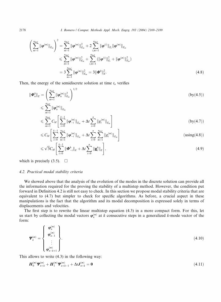
Then, the energy of the semidiscrete solution at time tn verifies

kUhnkE ¼

Xndofm¼1

kuðmÞn k2Em

!1=2

ðbyð4:5ÞÞ

6

Xndofm¼1

kuðmÞn kEm

6

Xndofm¼1

CM

Xk1

i¼0

kuðmÞi kEm

"þ Dt

Xni¼0

kgðmÞi kEm

#ðbyð4:7ÞÞ

6CM

Xk1

i¼0

Xndofm¼1

kuðmÞi kEm

"þ Dt

Xni¼0

Xndofm¼1

kgðmÞi kEm

#ðusingð4:8ÞÞ

6

ffiffiffi3

pCM

Xk1

i¼0

kUhikE

"þ Dt

Xni¼0

kghi kE

#; ð4:9Þ

which is precisely (3.5).

4.2. Practical modal stability criteria

We showed above that the analysis of the evolution of the modes in the discrete solution can provide all

the information required for the proving the stability of a multistep method. However, the condition put

forward in Definition 4.2 is still not easy to check. In this section we propose modal stability criteria that are

equivalent to (4.7) but simpler to check for specific algorithms. As before, a crucial aspect in these

manipulations is the fact that the algorithm and its modal decomposition is expressed solely in terms of

displacements and velocities.The first step is to rewrite the linear multistep equation (4.3) in a more compact form. For this, let

us start by collecting the modal vectors uðmÞn at k consecutive steps in a generalized k-mode vector of the

form:

WðmÞn ¼

uðmÞn

uðmÞn1

..

.

uðmÞnkþ1

8>>>>><>>>>>:

9>>>>>=>>>>>;: ð4:10Þ

This allows to write (4.3) in the following way:

HðmÞ0 W

ðmÞnþk þH

ðmÞ1 W

ðmÞnþk1 þ DtJ ðmÞ

nþk ¼ 0 ð4:11Þ


for two matrices HðmÞ1 ;H

ðmÞ1 of even dimension in terms of the modal amplification matrices LðmÞ

i :

HðmÞ0 ¼

LðmÞk LðmÞ

k1 LðmÞk2 . . . LðmÞ

1

0 1 0 . . . 0

0 0 1 . . . 0

..

. ... ..

. . .. ..

.

0 0 0 . . . 1;

266666664

377777775; H

ðmÞ1 ¼

0 0 . . . 0 LðmÞ0

1 0 . . . 0 0

0 1 . . . 0 0

..

. ... . .

.0 ..

.

0 0 . . . 1 0;

2666664

3777775; ð4:12Þ

and one vector Jnþk of modal forces:

JðmÞnþk ¼

gðmÞnþk þ gðmÞnþk1 þ þ gðmÞn

0

..

.

0

8>>><>>>:

9>>>=>>>;: ð4:13Þ

With this notation, one can write the solution at time tnþk as

WðmÞnþk ¼ AðmÞW

ðmÞnþk1 þ DtG ðmÞ

nþk; ð4:14Þ

where the modal amplification matrix AðmÞ and the forcing vector GðmÞnþk are of the form

AðmÞ ¼ ðH ðmÞ0 Þ1

HðmÞ1 ; G

ðmÞnþk ¼ ðH ðmÞ

0 Þ1JðmÞnþk: ð4:15Þ

Example 4.4. For the HHT method, the amplification matrix takes the form

AðmÞ ¼ ðLðmÞ2 Þ1 ðLðmÞ

2 Þ1LðmÞ1

0 1

0 LðmÞ

0

1 0

; ð4:16Þ

where the 2 · 2 blocks LðmÞi are given in (4.4).

Since every generalized k-mode vector contains the amplitude and velocity of the corresponding mode at

k successive steps, its total energy can be defined as

kWðmÞn k2Em

¼Xk1

i¼0

kuðmÞnik

2Em: ð4:17Þ

By abuse of notation we have employed the same symbol k kEmto denote the mth modal norm of one mode

and also of k consecutive modes. The notation introduced allows to write the modal formulation of the

multistep method in a very compact form but, more importantly, to prove Theorem 4.5 which will be the

basis of the stability criteria to be proposed. This theorem gives a simple condition on the amplification

matrix which guarantees modal stability of the time integration scheme.

Theorem 4.5. A time integration scheme of the type (2.12) is unconditionally modal stable if and only if thereexists a constant Ca, independent of h;m and N such that

kðAðmÞÞnkEm6Ca ð4:18Þ

for all n, with 06 n6N . The norm employed is the matrix norm associated with (4.17).


Proof. The proof employs, once more, standard arguments for the analysis of multistep methods and takes

into account the fact that the integration takes place in the context of the discretization of a partial dif-

ferential equation. In order to obtain the correct bounds in the modal energy norm k kEm, it is crucial to

have the method expressed as in (4.14) with no modal accelerations or higher order derivatives coming into

play.

To prove that condition (4.18) is sufficient for unconditional modal stability note that by applying

recursively (4.14), the generalized modal vector WðmÞn can be expressed as

WðmÞn ¼ AðmÞW

ðmÞn1 þ DtGn

¼ AðmÞðAðmÞWðmÞn2 þ DtG ðmÞ

n1Þ þ DtG ðmÞn :

¼ ðAðmÞÞ2ðAðmÞWðmÞn3 þ DtG ðmÞ

n2Þ þ DtðG ðmÞn þ AðmÞG

ðmÞn1Þ

..

.

¼ ðAðmÞÞnWðmÞ0 þ DtðG ðmÞ

n þ AðmÞGðmÞn1 þ þ ðAðmÞÞn1

GðmÞ1 Þ:

ð4:19Þ

Taking norms of both sides and using the triangle inequality it follows that

kWðmÞkEm6 kðAðmÞÞnkEm

kWðmÞ0 kEm

þ DtðkG ðmÞn kEm

þ þ kðAðmÞÞn1kEmkG ðmÞ

1 kEmÞ: ð4:20Þ

Using the definitions of the generalized modal vector WðmÞ and forcing vector G ðmÞn , the bound (4.18), and

employing (4.20) one gets

kuðmÞn kEm

6 kWðmÞn kEm

6Ca kWðmÞ0 kEm

þ Dtðk þ 1Þ

Xni¼0

kgðmÞi kEm

!

6Caðk þ 1ÞXk1

i¼0

kuðmÞi kEm

þ Dt

Xni¼0

kgðmÞi kEm

!: ð4:21Þ

Taking the supremum with respect to n and m of both sides we obtain precisely the condition for modal

stability (4.7).

We prove that condition (4.18) is also necessary for unconditional modal stability by contradiction.

Assume that a multistep scheme verifies (4.7) but not (4.18). If this last condition is not met, for a certainmesh size h there exists a mode m and a time step n such that

kðAðmÞÞnk2Em> 2kC2

M ; ð4:22Þ

where k is the number of steps of the method and CM is the constant appearing in (4.7). Let WðmÞ be the k-

modal vector of unit energy norm that maximizes the energy norm of the matrix ðAðmÞÞn, i.e., the vector suchthat

kðAðmÞÞnkEm:¼ max

kWkEm¼1kðAðmÞÞnWkEm

¼ kðAðmÞÞnWðmÞ kEm

: ð4:23Þ

Also, define WðmÞn as the vector of modal solutions at times t ¼ tn; tn1; . . . ; tnkþ1 with initial conditions WðmÞ

and zero external forces. If the integration method is modally stable then, according to Definition 4.2 and

the fact that the external forces are zero,


kuðmÞn k2Em

6C2M

Xk1

i¼0

kuðmÞi kEm

" #2¼ C2

MkWðmÞ kEm

¼ C2M ð4:24Þ

for all 06 n6N . Finally, starting from Eq. (4.22), using the definitions of the vector WðmÞn , the energy norm

(4.17) and the inequality (4.24) we obtain

2kC2M < kðAðmÞÞnk2Em

¼ kðAðmÞÞnWðmÞ k2Em

¼ kWðmÞn k2Em

¼Xk1

i¼0

kuðmÞn1k

2

Em6 kC2

M ð4:25Þ

which is a contradiction. We conclude that if a linear multistep method is modally stable then (4.18) must

hold. h

The previous theorem tells that the stability of linear multistep methods can be determined if a uniform

bound is found for the powers of every amplification matrix AðmÞ and, in particular, when h and Dt go to

zero or equivalently when N and ndof go to infinity. If the bound (4.18) holds only for certain values of theCourant number then the method is said to be conditionally modal stable.

To facilitate the algebra and avoid using the modal energy norm, a diagonal matrix Cm of dimensions

2k 2k is defined as Cm ¼ diag½1;xm; 1;xm; . . . ; 1;xm. It can be verified that

kðAðmÞÞnkEm¼ kðCmAmC

1m ÞnkEm

¼ kCmðAmÞnC1m kEm

¼ kðAmÞnk2 ð4:26Þ

for a modified modal amplification matrix Am ¼ C1m AðmÞCm which is non-dimensional and depends only on

the non-dimensional frequency Xm ¼ xmDt. Writing Am ¼ AðXmÞ and using the identity (4.26), the sta-

bility condition (4.18) can be rewritten in an equivalent form which instead of the modal energy norm

employs the matrix two-norm:

ð4:18Þ () sup16m6 ndof06 n6N

kAðXmÞnk2 6Ca: ð4:27Þ

Theorem 4.5, or the equivalent condition (4.27), states that the problem of determining the stability of a

linear multistep method is equivalent to determining if the set of all the possible modal amplification

matrices is uniformly power-bounded. Since the modified amplification matrices depend only on the non-

negative parameter X ¼ xDt, to verify stability it suffices to study the uniform power boundedness of the

matrix set

M1 ¼ fAðXÞ;X 2 ð0;1Þg: ð4:28ÞThe power boundedness of a matrix set was addressed, for example, in [21, Chapter 4], [22] and [6]. We

refer to these references for an extended discussion. The only sufficient condition for uniform power

boundedness that will be needed for the examples of Section 5 is based in the following theorem of [6].

Theorem 4.6. Let M be a set (finite or infinite) of matrices with finite dimensions. If

SC1: all the matrices A in M are spectrally stable 1andSC2: the set M is closed and bounded, then the set M is uniformly power-bounded, i.e., there exists a constant

C such that

1 A matrix is spectrally stable if its spectral radius q (the maximum modulus of its eigenvalues) is less or equal to 1 and eigenvalues of

modulus 1 are simple.


kAkn2 6C ð4:29Þfor all nP 0 and all A in M.

The previous theorem provides a sufficient condition for the stability analysis of specific time-steppingalgorithms, as the examples in Section 5 show. Given a time integration algorithm, one needs to calculate

the modified amplification matrix A as a function of the non-dimensional frequency X and possibly some

algorithmic parameters and then establish the power boundedness of the corresponding set M1 with the

aid of Theorem 4.6.

Remark 4.7

ii(i) In some practical applications of stability analysis it might be simpler to study the power boundedness

of a larger set thanM1, for example its closure. The power boundedness of the larger set will imply thesame property of its subset M1.

i(ii) The classical spectral stability criterion referred to in Section 1 is precisely condition SC1. Since con-

dition SC2 cannot be ignored for Theorem 4.6 to hold, one must conclude that the classical spectral

stability condition is not enough for power boundedness of the set of amplification matrices (and hence

stability) unless this set is closed and bounded.

(iii) Another difference between the stability criteria presented in this section and the classical spectral sta-

bility condition is that the latter has been applied to a different amplification matrix relating successive

modal displacement, velocities and higher order rates. See, for example, [2,14] and [5].

In summary, in this section we have shown that the uniform energy stability of a time stepping algorithm

can be equivalently expressed in terms of the its modal stability which, in turn, can be stated as the property

of uniform power boundedness of a certain matrix set. Theorem 4.6 is employed as an example of a suf-

ficient condition for modal (and hence global) stability.

5. Examples

In this section we apply some of the criteria of Section 4 to study the uniform modal stability of

three linear multistep schemes when they are applied to the integration of the equations of elastodynam-

ics. The results presented differ in some cases from those obtained with the classical spectral stability cri-

terion.

5.1. Stability of the HHT method

The first example considered examines the HHT method [14]. This method, already presented in

Examples 2.4, 4.1 and 4.4, is, according to the classical spectral analysis, unconditionally stable for the

parameter choice 126 a6 1. In practical use, only the range 0:76 a6 1 is employed since it is for these

parameter values that the numerical dissipation of the method is maximized. When a ¼ 1 the HHT method

reduces to the trapezoidal rule, which can be written as a one-step method and was analyzed in [22] and will

not be considered hereafter.

To study the stability of the HHT method we will first consider the sufficient condition (4.27). Before

this, we need to obtain the modified amplification matrix A which can be calculated from its definition(4.26) and the expression of the amplification matrix AðmÞ given in (4.16). After some straightforward

manipulations, the one-step amplification matrix obtained is


AðXÞ ¼

1 bX2 þ að2b 1=2ÞX2

1þ abX2

X

1þ abX2

ð1 aÞðb 1=2ÞX2

1þ abX20

X aðc 1Þ cþ a2ðc=2 bÞX2

1þ abX2

1þ aðb cÞX2

1þ abX2

Xð1 aÞ c 1þ aðc=2 bÞX2

1þ abX20

1 0 0 0

0 1 0 0

26666666664

37777777775;

ð5:1Þwhere the parameters ðb; cÞ are related to a according to (2.15) and X ¼ xDt.

To decide whether the matrix AðXÞ verifies the stability condition (4.27) we make use of Theorem 4.6.

To test the condition SC1, we start by calculating the spectral radius q of the amplification matrix A as a

function of the algorithmic parameter a and the non-dimensional frequency X. Fig. 1 plots the value of the

spectral radius of matrix AðXÞ for three values of the parameter a. The results obtained are identical tothose of the spectral analysis of the original paper [14] which proved that the method is spectrally stable for126 a6 1. However, the set M1 of all the possible amplification matrices is not bounded when a 6¼ 1, which

is needed for condition SC2 to hold. To see this, observe that for this choice of the parameter a, the ð2; 1Þand ð2; 3Þ components of the amplification matrix grow without bound as X goes to infinity. We conclude

that even though each of the amplification matrices of the HHT method is spectrally stable when

1=26 a < 1, we cannot guarantee the unconditional stability of the method for this parameter choice.

To further analyze the method, we consider now the modal stability condition (4.27) directly. It is

difficult to work analytically with this expression but numerical computations can be used to verify it. InFig. 2 the 2-norm of powers of the modal amplification matrix AðXÞ is depicted when a ¼ 0:8. The figureillustrates that for any given non-dimensional frequency X the norm of the corresponding amplification

matrix is bounded, but a uniform bound does not exist for all values of X. The first fact is a consequence of

the spectral stability of each individual amplification matrix. The second aspect results from the

unboundedness of the set M1. Similar results hold for other values of the parameter a in the interval of

interest 1=26 a < 1.

These results show that the HHT method is not unconditionally energy stable in the sense of Definition

3.1 when a < 1. For any given spatial discretization of the governing equations the energy of the fully

0.5

0.6

0.7

0.8

0.9

1

0 50 100 150 200

Ω

α = 0 .9α = 0 .8α = 0 .7

ρ

Fig. 1. Spectral radius q of the amplification matrix (5.1) of the HHT method for three values of the parameter a.

0 50 100 150 200 250 300 350 400Ω

Ω

010

2030

4050

048

121620

Fig. 2. HHT method with a ¼ 0:8. Two-norm of amplification matrix (5.1) powers.


discrete solution obtained with this method will always remain bounded. However, for arbitrary initial

conditions and forces, this bound can grow without control as the spatial mesh is refined.This fact is closely related to the so-called overshoot phenomenon (see e.g. [12]), which appears in the first

time steps of the integration when certain time-stepping algorithms, such as the HHT, are employed.

Considering again a fixed system of semidiscrete equations, the energy of high frequency modes tends to

grow during the first time steps (see Fig. 2 for large X and small n), but eventually is damped out (see again

Fig. 2 for large values of X and n) by means of artificial numerical dissipation. This undesired initial

growth––the overshoot––can be alleviated if, for the same spatial discretization, the time step size Dt isreduced. In this case, the maximum value of X is reduced proportionally to Dt and also the growth of the

high frequency modes (observe how in Fig. 2 the bounds of the amplification matrix are smaller for smallerX). However if the spatial mesh is refined, higher frequency modes can appear in the solution. If the time

step size is kept constant then the overshoot effect of the new solution will become even stronger since the

maximum value of X will increase and Fig. 2 shows that the maximum modal growth increases with X.If only a finite number of frequencies takes part of the solution, then the closure of the set of all possible

amplification matrices is closed and bounded, hence spectral stability of the individual amplification

matrices is sufficient for unconditional stability of the method according to Theorem 4.6. This happens, for

example, in the solution of any ordinary differential equation of the form (2.9). In this case, we have shown

that when the time step Dt goes to zero, the discrete solution obtained with the HHT method will convergeto the exact solution of the ordinary differential equation. However, after the analysis presented, the same

result cannot be extrapolated to the solution of the IBVP of elastodynamics. Under arbitrary initial con-

ditions and forces, it cannot be claimed that the solution obtained with the HHT as both h and Dt go to zero

is unconditionally energy stable, and hence it converges to the exact solution of the partial differential

equations.

In practical computations, the analyst often chooses only one mesh for the calculations. In this case,

irrespective of the time step size selected, the energy of the solution computed with the HHT method and

1=26 a6 1 will remain bounded in accordance with the classical spectral stability analysis. However, theanalysis presented shows that the errors in the solution may be larger than those obtained with a coarser

mesh or, in other words, that refining the spatial mesh could make the fully discrete solution worse.

5.2. Stability of Houbolt’s method

As a second example, we consider Houbolts method, another linear multistep for the second order

equation of elastodynamics. Following the same strategy as in Section 5.1, we study if the method satisfies a

necessary and sufficient condition for unconditional modal stability.


The method is usually presented in the form of a three field method with equations:

MAnþ1 þKUnþ1 ¼ fnþ1;

Dt2Anþ1 ¼ 2Unþ1 5Un þ 4Un1 Un2;

DtVnþ1 ¼11

6Unþ1 3Un þ 3

2Un1 3Un2: ð5:2Þ

The equations can be rewritten in the form of a linear three step method of the type (2.12). The modal

amplification matrices obtained after a straightforward manipulation are

LðmÞ3 ¼

2þ X2m 0

11

6Dt1

24

35; LðmÞ

2 ¼5 0

3

Dt0

24

35; LðmÞ

1 ¼4 0

3

2Dt0

24

35; LðmÞ

0 ¼1 0

1

3Dt0

24

35;

ð5:3Þand the modal amplification matrix is

AðmÞ ¼LðmÞ3 LðmÞ

2 LðmÞ1

0 1 0

0 0 1

24

351

0 0 LðmÞ0

1 0 0

0 1 0

24

35

¼ðLðmÞ

3 Þ1LðmÞ2 ðLðmÞ

3 Þ1LðmÞ1 ðLðmÞ

3 Þ1LðmÞ0

1 0 00 1 0

24

35: ð5:4Þ

The modified amplification matrix A can be obtained from this last equation and its definition (4.26). After

some algebraic manipulations, one gets

AðXÞ ¼ 1

2þ X2

5 0 4 0 1 0

19 18X2

6X0

26þ 9X2

6X0

7 2X2

6X0

1 0 0 0 0 0

0 1 0 0 0 0

0 0 1 0 0 0

0 0 0 1 0 0

26666666666664

37777777777775: ð5:5Þ

To see if Houbolts method is spectrally stable we start by considering the conditions of Theorem 4.6 which

are sufficient for stability. For every value of X the spectral radius q is less than 1, which verifies the stability

condition SC1. Fig. 3 depicts the value of the spectral radius of the method for an interval of the non-

dimensional frequency X ¼ xDt. To prove the uniform stability of the method it suffices now to show that

the set M1 of all amplification matrices is closed and bounded. But, for this method, the amplificationmatrix A becomes unbounded when X ! 0 since its terms ð2; 1Þ, ð2; 3Þ and ð2; 5Þ grow without control in

this limit. We conclude that the spectral analysis of Houbolts method alone does not guarantee its

unconditional stability.

As in Section 5.1, the modal condition (4.27) cannot be checked analytically and Fig. 4 depicts the norm

of the powers of the amplification matrix for an interval of the non-dimensional frequency X. The figure

confirms that, even though for each value of X the corresponding amplification matrix is power-bounded,

these norms grow when X approaches zero. Hence, the set M1 is not uniformly power bounded and the

method cannot be unconditionally stable.

0

0.2

0.4

0.6

0.8

1

0 40 80 120 160 200Ω

ρ

Fig. 3. Spectral radius q of the amplification matrix of Houbolts method.

0 0.002 0.004 0.006 0.008 0.01Ω 010

2030

4050

0

2500

5000

7500

10000

Fig. 4. Houbolts method. Two-norm of amplification matrix (5.5) powers.


5.3. Stability of Park’s method

Finally, we consider Parks method which can be formulated as a linear three step method for the second

order equation (2.12) defining the matrices

Lh3 ¼

1 3

5Dt1

3

5DtM1K 1

264

375; Lh

2 ¼ 3

21; Lh

1 ¼3

51; Lh

0 ¼1

101: ð5:6Þ

The form of the modal amplification matrix is identical to (5.4) and, after substitution of the modal matrices

corresponding to (5.6), one obtains the modified amplification matrix for the one step form of the method:

AðXÞ ¼

75

50þ 18X2

45X

50þ 18X2

15

25þ 9X2

9X

25þ 9X2

5

50þ 18X2

3X

50þ 18X2

45X

50þ 18X2

75

50þ 18X2

9X

25þ 9X2

15

25þ 9X2

3X

50þ 18X2

5

50þ 18X2

1 0 0 0 0 0

0 1 0 0 0 0

0 0 1 0 0 0

0 0 0 1 0 0

26666666666664

37777777777775

ð5:7Þ

0

0.2

0.4

0.6

0.8

1

0 40 80 120 160 200Ω

ρ

Fig. 5. Spectral radius q of the modal amplification matrix for Parks method.

050

100150

200 Ω

010

2030

4050

012345

Fig. 6. Parks method. Two-norm of amplification matrix (5.7) powers.


As in the previous two examples, we start by considering the conditions provided by Theorem 4.6. In Fig. 5,

the spectral radius of (5.7) is depicted and confirms SC1, i.e., the unconditional spectral stability of every

matrix in the set of amplification matrices M1. Moreover, in this case, the closure of the infinite matrix set

M1 is closed and bounded, and thus SC2 is verified. By Theorem 4.6, the set M1 is uniformly power

bounded and by Theorem 4.5 the method is stable. Fig. 6 shows the 2-norm of the powers of the matrix

AðXÞ verifying that there is a uniform bound for all these norms, in contrast with the amplification

matrices of the previous two methods.

6. Summary and conclusions

We have presented an analysis of the numerical discretization of the problem of elastodynamics resulting

from the use of finite elements in space and linear multistep methods in time with emphasis in the stability

of the time integration. The results generalize some of those presented in [22] allowing the analysis of the

most common time integration schemes employed in linear solid and structural dynamics which are often

linear multistep methods for the second order differential equation of the problem.


The stability of the time integration is done in the context of the energy norm and an appropriatestability notion is given as a the uniform bound of the fully discrete solution.

The spectral decomposition of the equations provides useful criteria that can be applied to specific time

stepping methods. The fundamental observation is that in order to obtain valid modal stability conditions the

equations must be written only in terms of the displacements and velocities of the solution and the bounds

obtained must be uniform in the mesh size and time step. Starting from these considerations and employing

standard error analysis techniques for multistep methods, necessary and sufficient conditions for uniform

stability are obtained. These conditions are valid for arbitrary loading and initial conditions, and are stronger

than the classical spectral stability criterion, which is shown to be necessary but not sufficient for stability.Using the modal criteria obtained, we analyze the stability of three specific multistep integrators: the

HHT method, Houbolts method and Parks method. Previous spectral analysis claimed that the three

methods are unconditionally stable but the stability criteria identified through the analysis indicate that

only the third of these schemes can be shown to be unconditionally stable and thus convergent.

Acknowledgements

The author would like to thank Prof. Juan C. Garcıa Orden and Prof. Jose M. Goicolea for their

interest, suggestions and helpful comments.

References

[1] G.A. Baker, J.H. Bramble, Semidiscrete and single step fully discrete approximations for second order hyperbolic equations,

RAIRO Numer. Anal. 13 (1979) 75–100.

[2] K.J. Bathe, E.L. Wilson, Stability and accuracy analysis of direct integration methods, Earthquake Engrg. Struct. Dynam. 1

(1973) 283–291.

[3] G. Bazzi, E. Anderheggen, The q-family of algorithms for time-step integration with improved numerical dissipation, Earthquake

Engrg. Struct. Dynam. 10 (1982) 537–550.

[4] T. Belytschko, An overview of semidiscretization and time integration procedures, in: T. Belytschko, T.J.R. Hughes (Eds.),

Computational Methods for Transient Analysis, Elsevier Scientific Publishing Co., Amsterdam, 1983, pp. 67–155.

[5] J. Chung, G. Hulbert, A time integration algorithm for structural dynamics with improved numerical dissipation: the generalized-

a method, J. Appl. Mech. 60 (1993) 371–375.

[6] G. Dahlquist, H. Mingyou, R. LeVeque, On the uniform power-boundedness of a family of matrices and the application to one-

leg and linear multistep methods, Numer. Math. 42 (1983) 1–13.

[7] V.A. Dougalis, Multistep-Galerkin methods for hyperbolic equations, Math. Comput. 33 (1979) 563–584.

[8] C.W. Gear, Numerical initial value problems in ordinary differential equations, in: Automatic Computation, Prentice-Hall,

Englewood Cliffs, NJ, 1971.

[9] E. Gekeler, Linear multistep methods and Galerkin procedures for initial boundary value problems, SIAM J. Numer. Anal. 13

(1976) 536–548.

[10] M. Geradin, A classification and discussion of integration operators for transient structural response, Technical Report, AIAA

paper 74-105, AIAA 12th Aerospace Sciences Meeting, Washington, DC, 1974.

[11] T. Geveci, On the convergence of Galerkin approximation schemes for second-order hyperbolic equations in energy and negative

norms, Math. Comput. 42 (1984) 393–415.

[12] G.L. Goudreau, R.L. Taylor, Evaluation of numerical methods in elastodynamics, Comput. Methods Appl. Mech. Engrg. 2

(1973) 69–97.

[13] E. Hairer, S.P. Nørsett, G. Wanner, Solving ordinary differential equations. I. Nonstiff problems, in: Springer Series in

Computational Mathematics, vol. 8, 1st ed., Springer-Verlag, 1987.

[14] H.M. Hilber, T.J.R. Hughes, R.L. Taylor, Improved numerical dissipation for time integration algorithms in structural dynamics,

Earthquake Engrg. Struct. Dynam. 5 (1977) 283–292.

[15] J.C. Houbolt, A recurrence matrix solution for the dynamic response of elastic aircraft, J. Aeronaut. Sci. 17 (1950) 540–550.

[16] T.J.R. Hughes, Analysis of transient algorithms with particular reference to stability behavior, in: T. Belytschko, T.J.R. Hughes

(Eds.), Computational Methods for Transient Analysis, Elsevier Scientific Publishing Co., Amsterdam, 1983, pp. 67–155.


[17] T.J.R. Hughes, The Finite Element Method, Prentice-Hall Inc., Englewood Cliffs, NJ, 1987.

[18] J.D. Lambert, Numerical Methods for Ordinary Differential Systems, Wiley, Chichester, 1991.

[19] N.M. Newmark, A method of computation for structural dynamics, J. Engrg. Mech. Div., ASCE 85 (1956) 67–94.

[20] K.C. Park, Evaluating time integration methods for nonlinear dynamic analysis, in: T. Belytschko, T.L. Geers (Eds.), Finite

Element Analysis of Transient Nonlinear Behavior, AMD 14, ASME, New York, 1975, pp. 35–58.

[21] R.D. Richtmyer, K. Morton, Difference Methods for Initial Value Problems, John Wiley & Sons, Inc., New York, 1967.

[22] I. Romero, On the stability and convergence of fully discrete solutions in linear elastodynamics, Comput. Methods Appl. Mech.

Engrg. 191 (2002) 3857–3882.

[23] G. Strang, G.J. Fix, An Analysis of the Finite Element Method, Prentice-Hall, Englewood Cliffs, NJ, 1973.

[24] E. Wilson, A computer program for the dynamic stress analysis of underground structures, Technical Report, EERC Report No.

68-1, Division of Structural Engineering and Structural Mechanics, University of California, Berkeley, 1968.

stability analysis of linear multistep methods for classical elastodynamics

Documents