STABILITY ANALYSIS AND CONTROL DESIGN FOR HYBRID AC-DC MORE-

ELECTRIC AIRCRAFT POWER SYSTEMS

by

Xiao Li

Submitted to the Graduate Faculty of

Swanson School of Engineering in partial fulfillment

of the requirements for the degree of

Master of Science

University of Pittsburgh

2013

ii

UNIVERSITY OF PITTSBURGH

SWANSON SCHOOL OF ENGINEERING

This thesis was presented

by

Xiao Li

It was defended on

April 1, 2013

and approved by

Zhi-Hong Mao, Ph.D., Associate Professor, Department of Electrical and Computer Engineering

Gregory Reed, Ph.D., Associate Professor, Department of Electrical and Computer Engineering

Thomas McDermott, Ph.D., Assistant Professor, Department of Electrical and Computer Engineering

Thesis Advisor: Zhi-Hong Mao, Ph.D., Associate Professor, Department of Electrical and Computer

Engineering

iii

Copyright © by Xiao Li

2013

iv

STABILITY ANALYSIS AND CONTROL DESIGN FOR HYBRID AC-DC MORE-

ELECTRIC AIRCRAFT POWER SYSTEMS

Xiao Li, M.S.

University of Pittsburgh, 2013

This thesis studies the stability of a more-electric aircraft (MEA) power system with hybrid

converters and loads, and proposes a control design method using state feedback. The MEA is

aimed to replace the conventional nonelectric power in aircraft with electric power in order to

reduce the size and weight of the aircraft power system. This thesis considers a model of the

MEA power system consisting of the following components: converters with uncontrolled diodes

and controlled rectifiers, ideal constant power loads (CPL), and non-ideal CPL driven by

electromechanical actuators. The system has narrow stability range under the conventional two-

loop PI control. To improve control performance, a full-state feedback control method is

developed that can significantly increase the stability margin of the MEA power system.

v

TABLE OF CONTENTS

ACKNOWLEDGMENT ............................................................................................................. X

1.0 INTRODUCTION ........................................................................................................ 1

1.1 BACKGROUND .................................................................................................. 1

1.2 LITERATURE REVIEW ................................................................................... 3

1.2.1 General points ................................................................................................... 3

1.2.2 Generalized aircraft AC electrical power system architecture .................... 4

1.3 THESIS CONTRIBUTION ................................................................................ 6

2.0 METHMETICAL MODEL OF THE MEA POWER SYSTEM ............................ 8

2.1 POWER SYSTEM DEFINITIION .................................................................... 8

2.2 MODELLING OF SUB-SYSTEMS ................................................................... 9

2.2.1 Diode rectifier models .................................................................................... 10

2.2.2 Controlled rectifier model .............................................................................. 17

2.2.3 Electromechanical Actuator (EMA) models ................................................ 21

2.2.4 Ideal CPL load ................................................................................................ 27

2.2.5 Combined model of the whole studied system ............................................. 29

3.0 SIMULATION AND RESULTS ............................................................................... 32

3.1 STABILITY ANALYSIS .................................................................................. 32

3.2 APPLYING STATE FEEDBACK CONTROLLER ...................................... 36

vi

4.0 CONCLUSION ........................................................................................................... 38

APPENDIX A .............................................................................................................................. 39

APPENDIX B .............................................................................................................................. 43

BIBLIOGRAPHY ....................................................................................................................... 44

vii

LIST OF TABLES

Table 1. The parameters in the MEA architecture .......................................................................... 4

Table 2. Real part of the system eigenvalues with different power levels ................................... 33

Table 3. The system parameters.................................................................................................... 43

viii

LIST OF FIGURES

Figure 1. Generalized aircraft AC electrical power system architecture ....................................... 5

Figure 2. The power system studied ............................................................................................... 9

Figure 3. Diode rectifier ................................................................................................................ 10

Figure 4. 3-phase diode rectifier with overlap angle resistance.................................................... 12

Figure 5. The rectifier switching signal ........................................................................................ 13

Figure 6. The vector diagram for DQ transformation ................................................................... 14

Figure 7. The equivalent circuit of rectifier in dq frame ............................................................... 15

Figure 8. The equivalent circuit on d-q frame rotating at ωt+ϕ ................................................... 16

Figure 9. The simplified equivalent circuit of the power system ................................................. 16

Figure 10. The switching signal of a controlled rectifier .............................................................. 17

Figure 11. The vector diagram for DQ transformation ................................................................. 18

Figure 12. The combination system of the two rectifiers ............................................................. 19

Figure 13. The considered system ................................................................................................ 20

Figure 14. The schematic of the controllers .................................................................................. 20

Figure 15. The model for the motor .............................................................................................. 24

Figure 16. The standard motor drive control structure ................................................................. 24

Figure 17. The control structure neglecting d-axis current dynamic ............................................ 25

ix

Figure 18. Modulation index calculator ........................................................................................ 26

Figure 19. Block diagram of the non-linear EMA model for PM machine .................................. 27

Figure 20. DC source feeding a CPL load through a low-pass filter ............................................ 27

Figure 21. Ideal CPL load represented by a current source .......................................................... 28

Figure 22. The stable and unstable region for varying the power level ........................................ 33

Figure 23. Step response of the system at (PEMA=7kW, PCPL=25kW) .......................................... 34

Figure 24. Step response of the system at (PEMA=6kW, PCPL=26kW) .......................................... 35

Figure 25. Instability line for changing frequencies ..................................................................... 36

Figure 26. Step response after applying state feedback at PCPL=10kW and PEMA=50kW ............ 37

x

ACKNOWLEDGMENT

At the beginning, I would like to express my sincerely appreciate to my adviser Dr. Zhi-Hong

Mao. He always has a way to make me enjoy the research, and give me a strong support on

writing this paper. His journal club is excellent and instructive, from which I acquire countless

experience.

Secondly, I would like to express my sincerely appreciate to my committee members Dr.

Reed and Dr. McDermott for their support on my research. I learned a lot from Dr. Reed last two

years. His dedication and concentration affect me a lot.

Thirdly, I have to thank my parents for their great support on both financial and spiritual

aspect. Word cannot express my gratitude.

Last but not least, I would like to express my sincerely appreciate to my friends who

always encourage me and help me.

1

1.0 INTRODUCTION

1.1 BACKGROUND

The More-electric aircraft (MEA) concept is presented by military designer in World War II. It

underlines to use electric power to replace the conventional power energizing the non-propulsive

aircraft system. MEA is a trend for the future development of aircraft.

In a traditional aircraft, fossil energy is mainly converted into propulsive power to move

the aircraft. The remainder converted into four parts to power the non-propulsive aircraft system,

including hydraulic power, pneumatic power, mechanical power, and electrical power.

Hydraulic power, which is transferred from the central hydraulic pump, has to sustain its heavy

and inflexible piping, and the serious potential corrosive fluids leakage. Pneumatic power, which

is generated from the engines’ high pressure compressors, has the disadvantages of low

efficiency and difficult leak detection. In addition, each of these four systems has become more

and more complex, therefore the connections between them reduce the flexibility and become

more difficult. As a consequence, MEA tends to be a solution to reduce the aircraft power

systems’ size and weight and improve the fuel efficiency. It is believed that to develop an

electrical system have far more potential than a conventional one, in order to increase the energy

efficiency.

2

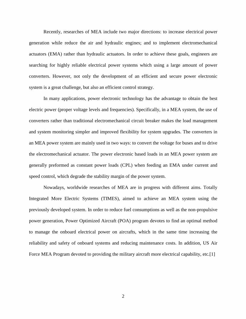
Recently, researches of MEA include two major directions: to increase electrical power

generation while reduce the air and hydraulic engines; and to implement electromechanical

actuators (EMA) rather than hydraulic actuators. In order to achieve these goals, engineers are

searching for highly reliable electrical power systems which using a large amount of power

converters. However, not only the development of an efficient and secure power electronic

system is a great challenge, but also an efficient control strategy.

In many applications, power electronic technology has the advantage to obtain the best

electric power (proper voltage levels and frequencies). Specifically, in a MEA system, the use of

converters rather than traditional electromechanical circuit breaker makes the load management

and system monitoring simpler and improved flexibility for system upgrades. The converters in

an MEA power system are mainly used in two ways: to convert the voltage for buses and to drive

the electromechanical actuator. The power electronic based loads in an MEA power system are

generally preformed as constant power loads (CPL) when feeding an EMA under current and

speed control, which degrade the stability margin of the power system.

Nowadays, worldwide researches of MEA are in progress with different aims. Totally

Integrated More Electric Systems (TIMES), aimed to achieve an MEA system using the

previously developed system. In order to reduce fuel consumptions as well as the non-propulsive

power generation, Power Optimized Aircraft (POA) program devotes to find an optimal method

to manage the onboard electrical power on aircrafts, which in the same time increasing the

reliability and safety of onboard systems and reducing maintenance costs. In addition, US Air

Force MEA Program devoted to providing the military aircraft more electrical capability, etc.[1]

3

1.2 LITERATURE REVIEW

This chapter reviews some important previous modeling works of power electronics and MEA

power systems.

1.2.1 General points

Power electronic loads are generally viewed as the constant power load having small-signal

negative impedance which degrades the system stability margin [2][3]. Many literatures studied

the model of ideal CPL without dynamics, but few of them consider about the dynamic CPL. In

reference [4], it studied controlled electromechanical actuators performed as a CPL having

dynamics.

There are three majority methods commonly used for analyzing the performance of

power converter systems: state space averaging (SSA) modeling method, average-value

modeling (AVM) method, and DQ transformation method. The generalized SSA modeling

method, using for analyzing many power converters in DC and AC distribution systems, has

represented by [5][6] in DC distribution systems, in the uncontrolled and controlled rectifiers in

single-phase [7], and in the 6 and 12 pulse diode rectifiers in three phase ac systems [8]. The

AVM method, which has been used for 6 and 12 pulse diode rectifiers, represented in [9].

Another widely used modeling methods for power converters and electromechanical actuator

control is the DQ-transformation method [10]. The priority of using DQ transformation method

can be seen by comparison with other two methods. The SSA modeling method leads to a

complex high-order mathematical model when applied to three-phase AC systems. The AVM

method is not easily applicable for vector-controlled converters because it cannot offer the

4

information on the AC side. The DQ transformation provides lower order system models than

SSA and is much easier to apply to a converter controlled in terms of rotation DQ frame aligned

with the grid voltage, and represents the converter as a transformer [11],

1.2.2 Generalized aircraft AC electrical power system architecture

Reference [12] presents an aircraft EPS architecture candidate, which is defined in the European

MOET project [13], as shown in Figure 1 (see next page). The parameters in this architecture are

described in Table 1.

Table 1. The parameters in the MEA architecture

Parameters Description

Req1, Leq1, Ceq1 the equivalent circuit of the transmission cable linking the generator bus

Gen bus and the HVAC bus

RTRUj, LTRUj, CTRUj AC cable linking HVAC bus and input terminal of the diode rectifier bus

rLFj, LFj, rCFj and CFj DC link filters for diode rectifiers

PidealCPL,De Ideal CPLs (represent other DC loads with regulated DC/DC power

converters by assuming an infinitely fast controller action)

PdynCPL,Dn Dynamics of CPL (represent the environmental control system fed

through the diode rectifiers)

Req2, Leq2, Ceq2 Transmission line linking the HVAC and the AC essential bus (AC ESS)

Rconk, Lconk Input circuit for active PWM controlled rectifiers

5

Table 1 (continued).

PidealCPL,Pg ,

PdynCPL,Pa

The ideal and dynamic CPLs represent other aircraft loads and EMAs

(ailerons, rudders, flaps, spoilers, and elevators, etc.)

RLb, LLb The wing de-icing connected to HVAC bus

Figure 1. Generalized aircraft AC electrical power system architecture [12]

6

In this architecture, the diode rectifiers convert the power for the environmental control

systems (ECS), which can be viewed as dynamics of CPL PdynCPL,Dn, and other DC loads. By

assuming an extremely small time constant of controller action, these DC loads can be viewed as

ideal CPLs PidealCPL,De. The pulse width modulation (PWM) controlled rectifiers feed the other

aircraft loads and electromechanical actuators (EMAs) such as elevators, ailerons, rudders, flaps,

and spoilers. The model of the controlled PWM rectifier was presented by K-N Areerak in [14].

1.3 THESIS CONTRIBUTION

As we mentioned in the previous section, the prospect of application for MEA are board and

many researches have been already in process. However, due to the huge power level

requirement in the modern aircraft power system, not only an efficient and secure power

electronics technology need to be developed but also a reliable control system of the power

electronics.

One of the big challenges for achieving MEA power system is the constant power load

(CPL). As we all known, the loads of the power electronic system can be viewed as constant

power loads, which significantly degrade the power system stability. A greater power level of

MEA system has narrower stability margin which causes the implementation of the MEA

impossible at present stage. The widely used control method for improve the system stability is

the conventional two-loop PI controller, which typically contains a current control loop as the

inner loop and a voltage or power control loop as the outer loop. However, when the two-loop PI

controller applies in the MEA system, it only provides a narrow stability margin. In this thesis, a

full-state feedback control method is used to enlarge the stability margin, and the result is

7

verified by MATLAB. Although it is a preliminary and theoretical work, it shows some

advantages for using the full-state feedback method to improve the system stability margin.

8

2.0 METHMETICAL MODEL OF THE MEA POWER SYSTEM

This Chapter presents the derivation of the mathematical model of the studied MEA power

system in detail.

2.1 POWER SYSTEM DEFINITIION

The power system studied is shown in Figure 2, which is simplified from the generalized aircraft

electrical power system architecture presented in [12]. To reduce the work of the modeling, this

thesis uses a controlled rectifier under double loop PI controllers rather than a PWM controller

and neglects the parameters of the transmission line between the AC bus and rectifiers. In Figure

2, the controlled rectifier drives an ideal constant load and the uncontrolled diode rectifier drives

a PM machine which can be viewed as a dynamic constant load.

9

Figure 2. The power system studied

2.2 MODELLING OF SUB-SYSTEMS

In this section, the specified process of the sub-systems modeling will be presented. There are

four components in the studied system:

1. Diode rectifier model;

2. Controlled rectifier model;

3. MEA model;

4. Ideal CPL model;

The diode rectifier model and the controlled rectifier model can be constructed as a

transformer by applying DQ transformation, which simplifies the analysis process.

10

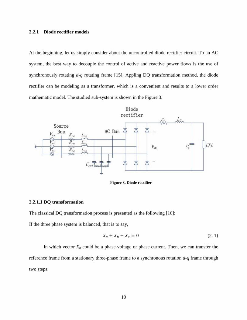
2.2.1 Diode rectifier models

At the beginning, let us simply consider about the uncontrolled diode rectifier circuit. To an AC

system, the best way to decouple the control of active and reactive power flows is the use of

synchronously rotating d-q rotating frame [15]. Appling DQ transformation method, the diode

rectifier can be modeling as a transformer, which is a convenient and results to a lower order

mathematic model. The studied sub-system is shown in the Figure 3.

Figure 3. Diode rectifier

2.2.1.1 DQ transformation

The classical DQ transformation process is presented as the following [16]:

If the three phase system is balanced, that is to say,

𝑋𝑎 + 𝑋𝑏 + 𝑋𝑐 = 0 (2. 1)

In which vector Xn could be a phase voltage or phase current. Then, we can transfer the

reference frame from a stationary three-phase frame to a synchronous rotation d-q frame through

two steps.

11

Firstly, applying Clark transformation equation,

𝑋𝛼𝛽 = 𝑋𝛼 + 𝑗𝑋𝛽 = 𝑘 �𝑋𝑎 + 𝑋𝑏𝑒−𝑗2𝜋3 + 𝑋𝑐𝑒

−𝑗4𝜋3 � (2. 2)

Where k is a constant number, we achieve the stationary 𝛼-𝛽 frame. In the matrix form:

�𝑋𝛼𝑋𝛽� = 𝑘 �

1 −12

− 12

0 √32

− √32

� �𝑋𝑎𝑋𝑏𝑋𝑐� (2. 3)

Secondly, applying Park transformation obtains the rotating d-q reference frames:

𝑿𝒅𝒒 = 𝑿𝜶𝜷𝑒−𝑗𝜃 (2. 4)

Now, we have the matrix form transformation equation of transferring directly from 𝑎𝑏𝑐 frame

to d-q frame by substitute (2.3) into (2.4):

�𝑋𝛼𝑋𝛽� = 𝑘 �

cos θ cos(θ − 2π3

) cos(θ + 2π3

)

−sinθ − sin(θ − 2π3

) − sin(θ + 2π3

)� �𝑋𝑎𝑋𝑏𝑋𝑐� = 𝑘𝑻 �

𝑋𝑎𝑋𝑏𝑋𝑐� (2. 5)

To calculate the vectors in d-q frame from 𝑎𝑏𝑐 frame, one can simply do the calculation:

𝑿𝜶𝜷 = 𝑘−1𝑻−1𝑿𝒂𝒃𝒄 (2. 6)

There are two typical value of k: 23 and�2

3. Each of them has corresponding physical meaning.

If k is chosen to be�23, which is usually called power invariant, or power conserving

convention, this result to the power calculated in the d-q reference frame and the power

calculated from 𝑎𝑏𝑐 reference frame will have the same magnitude. If k is chosen to be 23, which

is usually named as voltage invariant, or peak convention, this result to the vector quantity in d-q

reference frame is equal to the peak of phase quantity in 𝑎𝑏𝑐 reference frame.

The next section shows the process of using DQ transformation method to get the

equivalent circuit of the uncontrolled diode rectifier.

12

2.2.1.2 The equivalent circuit on d-q frame

It is best to begin with the analyzing of the rectifier with inductance effect on current

commutation. Then the whole equivalent circuit will be easily get by transfer the elements in the

𝑎𝑏𝑐 frame to d-q frame.

It is assumed that the converter is operating under the continues-conduction mode and the

three phases are balanced. According to Mohan’s power electronic text book [17], the inductance

Leq in the AC side causes an average DC voltage drop. This is because the inductance current

cannot change instantaneous when Leq is finite, which cause an overlap angle during the current

commutation process. This voltage drop can be represented as a resistance rμ located on the DC

side, depending on the system frequency ω, as shown in Figure 4.

Figure 4. 3-phase diode rectifier with overlap angle resistance [11]

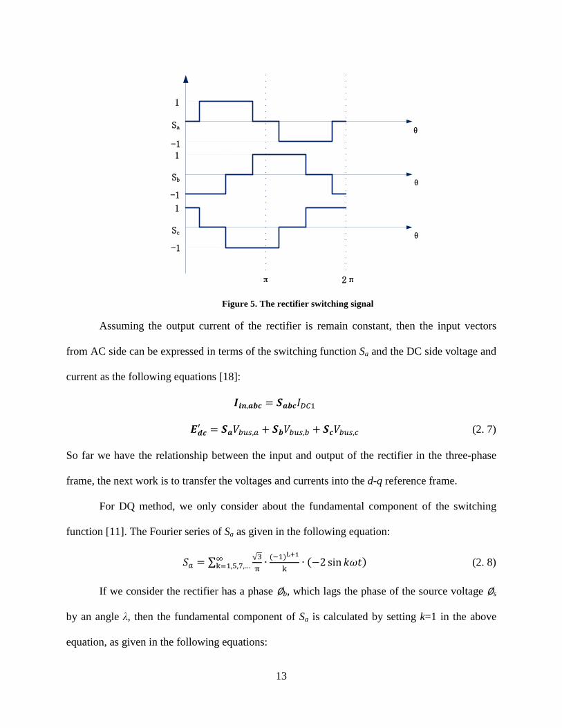
After introducing the equivalent variable resistance rμ, we can simply consider the diode

rectifier without concerning the effect of the overlap angle. The switching signal can be present

as shown in Figure 5.

13

1

1

1

-1

-1

-1

Sa

Sb

Sc

π 2π

θ

θ

θ

Figure 5. The rectifier switching signal

Assuming the output current of the rectifier is remain constant, then the input vectors

from AC side can be expressed in terms of the switching function Sa and the DC side voltage and

current as the following equations [18]:

𝑰𝒊𝒏,𝒂𝒃𝒄 = 𝑺𝒂𝒃𝒄𝐼𝐷𝐶1

𝑬𝒅𝒄′ = 𝑺𝒂𝑉𝑏𝑢𝑠,𝑎 + 𝑺𝒃𝑉𝑏𝑢𝑠,𝑏 + 𝑺𝒄𝑉𝑏𝑢𝑠,𝑐 (2. 7)

So far we have the relationship between the input and output of the rectifier in the three-phase

frame, the next work is to transfer the voltages and currents into the d-q reference frame.

For DQ method, we only consider about the fundamental component of the switching

function [11]. The Fourier series of Sa as given in the following equation:

𝑆𝑎 = ∑ √3π∙ (−1)L+1

k∙ (−2 sin𝑘𝜔𝑡)∞

k=1,5,7,… (2. 8)

If we consider the rectifier has a phase ∅b, which lags the phase of the source voltage ∅s

by an angle λ, then the fundamental component of Sa is calculated by setting k=1 in the above

equation, as given in the following equations:

14

𝑆𝑎 =2√3π

∙ (sin𝜔𝑡 − ∅𝑏)

𝑆𝑏 =2√3π

∙ �sin𝜔𝑡 −2𝜋3− ∅𝑏�

𝑆𝑐 = 2√3π∙ �sin𝜔𝑡 − 4𝜋

3−∅𝑏� (2. 9)

The vector diagram below shows the phase relationship among the voltage source Vs, switching

signal S and the input current Iin:

Figure 6. The vector diagram for DQ transformation

Notice that in the input current Iin is in phase with the input voltage Vbus. Vs is the peak amplitude

phase voltage of the source. S is the peak amplitude of switching signal. Now the vectors VS, Iin

and S can be presented into the DQ frame at rotating frequency ωt+ϕ using the power conserving

convention given in (2.10).

𝑽𝑺,𝒅𝒒 = �32𝑉𝑆𝑒𝑗(𝜙𝑠−𝜙)

𝑺𝒅𝒒 = �32�2√3

π� 𝑒𝑗(𝜙𝑠−𝜙)

𝑰𝒊𝒏,𝒅𝒒 = �32𝐼𝑖𝑛𝑒𝑗(𝜙𝑠−𝜙) (2. 10)

15

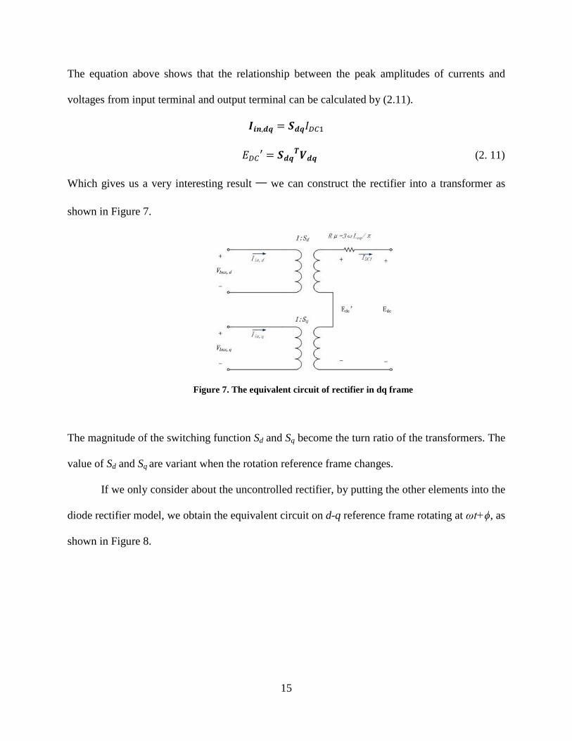
The equation above shows that the relationship between the peak amplitudes of currents and

voltages from input terminal and output terminal can be calculated by (2.11).

𝑰𝒊𝒏,𝒅𝒒 = 𝑺𝒅𝒒𝐼𝐷𝐶1

𝐸𝐷𝐶′ = 𝑺𝒅𝒒𝑻𝑽𝒅𝒒 (2. 11)

Which gives us a very interesting result ─ we can construct the rectifier into a transformer as

shown in Figure 7.

Figure 7. The equivalent circuit of rectifier in dq frame

The magnitude of the switching function Sd and Sq become the turn ratio of the transformers. The

value of Sd and Sq are variant when the rotation reference frame changes.

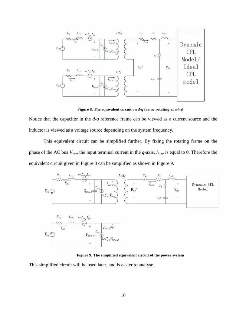
If we only consider about the uncontrolled rectifier, by putting the other elements into the

diode rectifier model, we obtain the equivalent circuit on d-q reference frame rotating at ωt+ϕ, as

shown in Figure 8.

16

Figure 8. The equivalent circuit on d-q frame rotating at ωt+ϕ

Notice that the capacitor in the d-q reference frame can be viewed as a current source and the

inductor is viewed as a voltage source depending on the system frequency.

This equivalent circuit can be simplified further. By fixing the rotating frame on the

phase of the AC bus Vbus, the input terminal current in the q-axis, Iin,q, is equal to 0. Therefore the

equivalent circuit given in Figure 8 can be simplified as shown in Figure 9.

Figure 9. The simplified equivalent circuit of the power system

This simplified circuit will be used later, and is easier to analyse.

17

2.2.2 Controlled rectifier model

This section presents the modeling of the controlled rectifier part applying DQ transformation

method. The analytical procedure of a controlled rectifier is very much like the procedure of the

diode rectifier. The different between them is the switching function [19] and the double PI

controller [20].

2.2.2.1 The equivalent circuit of controlled rectifier

By introducing an equivalent resistance rμ located in the DC side as we did in the last section, we

can simply apply the switching signal without considering the inductor effect. Assuming that the

harmonics of the actual switching signal can be ignored, the switching function of the controlled

rectifier is shown in Figure 10, in which α is the firing angle of thyristors.

Figure 10. The switching signal of a controlled rectifier

Mathematically, the fundamental component of the switching function can be written as:

𝑆𝑎 =2√3π

∙ (sin𝜔𝑡 + ∅ − α)

18

𝑆𝑏 = 2√3π∙ �sin𝜔𝑡 − 2𝜋

3+ ∅ − α�

𝑆𝑐 = 2√3π∙ �sin𝜔𝑡 − 4𝜋

3+ ∅ − α� (2. 12)

in which ∅ is a phase angle of the AC bus. The vector diagram for the DQ transformation is

shown in Figure 11.

Figure 11. The vector diagram for DQ transformation

The relationship between input and output terminal of the controlled rectifier is as the same as

the diode rectifier presented in the equation (2.10), (2.11). The switching function in the d-q

reference frame is given by:

𝐒𝐝𝐪𝟐 = �32∙ 2√3π� cos(ϕb − ϕ + α)− sin(ϕb − ϕ + α)� (2. 13)

The equivalent circuit of a controlled is the same as the model shown in Figure 7, except for the

turn ratio of the transformer Sdq. In a controlled rectifier, the firing angle α need to be taken into

consideration. The equivalent circuit for a controlled rectifier and other elements without

considering the uncontrolled diode rectifier subsystem can also be represented by Figure 8. The

difference is in a controlled rectifier model, the d-q frame is rotating at ωt+ϕ-α. This equivalent

circuit can also be simplified to eliminate the transformer in the q-axis by align the vector of

switching function S and the AC input current Iin with the d-axis. However, in order to get the

19

mathematic model for the whole system, we need to combine the two kinds of converters

together, which require that both the diode rectifier and the thyristor rectifier select a same d-q

reference frame. Then the model for the combination system of the two rectifiers can be

presented as shown in Figure 12

.

Figure 12. The combination system of the two rectifiers

From Figure 12 we can see that the total input current in d-q frame Iin,d and Iin,q are equal to the

sum of the diode rectifier input terminal current and the controlled rectifier input terminal current

in d-q frame correspondingly

2.2.2.2 Controllers of the system

This section presents the mathematic model for the controllers of the controlled rectifier system

[20]. The subsystem studied is as shown in Figure 13.

20

Figure 13. The considered system

The schematic of the controllers is as shown in Figure 14. It has two PI controllers cascaded, the

first one regulates the output voltage of the converter, and the second one regulates the DC

current.

Figure 14. The schematic of the controllers

In Figure 14, V* represents the reference voltage across the DC side resistor rF and inductor LF.

This schematic contains two control loops: the inner loop is the current loop, and the outer loop

is the voltage loop. Parameters Idc and Idc* represents the actual and reference value of the current

in DC side current, respectively. Vout and Vout* represents the actual and reference value of the

DC voltage, respectively. The parameters Kpv and Kiv are the proportional and integral gains of

the voltage, and Kpi and Kii are gains of the current. These gains of the PI controller can be

21

determined by classical method [19], or using ATS (Adaptive Tabu Search) and ABC (Artificial

Bee Colony) method [21].

2.2.3 Electromechanical Actuator (EMA) models

In this section, the EMA model with controllers is illustrated. The first part gives the physical

model of the motor and the second part provides the vector-controller of EMA.

2.2.3.1 Physical model of the PM machine

At the beginning, let us take a review on the principle of AC machine.

In an AC machine, assuming a three-phase balanced power supply in the three-phase

stator winding, the magnetic field is rotating and sinusoidally distributed in the air gap [22]. If

we give the definition for the following parameters:

P=number of poles of the machine;

ωr=the rotor mechanical speed (r/s);

ωe=the stator electrical speed (r/s);

ia,b,c= phase currents in the three-phase stator winding;

Im=the magnitude of the phase current;

N=number of turns in a phase winding;

Then ia,b,c are given as:

𝑖𝑎 = 𝐼𝑚cos𝜔𝑒𝑡

𝑖𝑏 = 𝐼𝑚cos �𝜔𝑒𝑡 −2𝜋3�

𝑖𝑐 = 𝐼𝑚cos �𝜔𝑒𝑡 + 2𝜋3� (2. 14)

22

Each phase of currents results in a magnetomotive force (MMF). At a particular angle θ, the

MMFs generated by phase currents are given in (2.15):

𝐹𝑎(𝜃) = 𝑁𝑖𝑎cos𝜃

𝐹𝑏(𝜃) = 𝑁𝑖𝑏cos �𝜃 − 2𝜋3�

𝐹𝑐(𝜃) = 𝑁𝑖𝑐cos �𝜃 + 2𝜋3� (2. 15)

Therefore, the total MMF at angle θ is given as:

F(θ) = 𝐹𝑎(𝜃) + 𝐹𝑏(𝜃) + 𝐹𝑐(𝜃)

= 𝑁𝑖𝑎cos𝜃 + 𝑁𝑖𝑏co s �𝜃 − 2𝜋3� + 𝑁𝑖𝑐cos �𝜃 + 2𝜋

3� (2. 16)

Substitute (2.14) into (2.16) gives:

𝐹(𝜃, 𝑡) = 𝑁𝐼𝑚[cos𝜔𝑒𝑡cos𝜃 + cos �𝜔𝑒𝑡 −2𝜋3� cos �𝜃 − 2𝜋

3�

+ cos �𝜔𝑒𝑡 + 2𝜋3� cos �𝜃 + 2𝜋

3�] (2. 17)

Simplifying equation (2.17) results in:

𝐹(𝜃, 𝑡) = 32𝑁𝐼𝑚 cos(𝜔𝑒𝑡 − 𝜃) (2. 18)

This sweeping magnetic field subjects the rotation of the rotor.

In this study case, we use a PM machine as the driver. A PM synchronous machine uses a

permanent magnet as the rotor instead of the dc field windings in the IM machine. It can be

viewed as a special case of inductor drives. There are several advantages to apply a PM machine:

to eliminate the field copper loss, has higher power density, has lower rotor inertia, and has more

robust construction of the rotor. In general, although its cost is higher, a PM machine has higher

efficiency than an IM machine.

To analyse the dynamic model of the PM drive, the DQ transformation is applying again.

The steady-state analysis of PM machine is the same as a wound field machine except that the

23

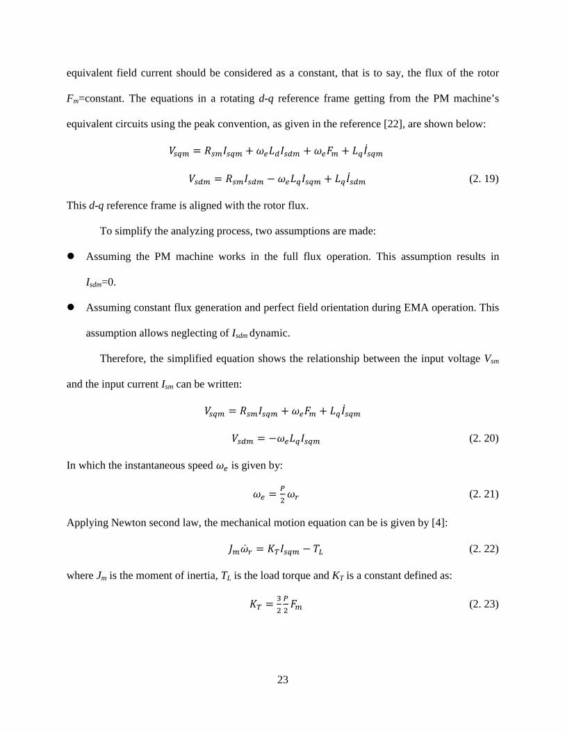
equivalent field current should be considered as a constant, that is to say, the flux of the rotor

Fm=constant. The equations in a rotating d-q reference frame getting from the PM machine’s

equivalent circuits using the peak convention, as given in the reference [22], are shown below:

𝑉𝑠𝑞𝑚 = 𝑅𝑠𝑚𝐼𝑠𝑞𝑚 + 𝜔𝑒𝐿𝑑𝐼𝑠𝑑𝑚 + 𝜔𝑒𝐹𝑚 + 𝐿𝑞𝐼�̇�𝑞𝑚

𝑉𝑠𝑑𝑚 = 𝑅𝑠𝑚𝐼𝑠𝑑𝑚 − 𝜔𝑒𝐿𝑞𝐼𝑠𝑞𝑚 + 𝐿𝑞𝐼�̇�𝑑𝑚 (2. 19)

This d-q reference frame is aligned with the rotor flux.

To simplify the analyzing process, two assumptions are made:

Assuming the PM machine works in the full flux operation. This assumption results in

Isdm=0.

Assuming constant flux generation and perfect field orientation during EMA operation. This

assumption allows neglecting of Isdm dynamic.

Therefore, the simplified equation shows the relationship between the input voltage Vsm

and the input current Ism can be written:

𝑉𝑠𝑞𝑚 = 𝑅𝑠𝑚𝐼𝑠𝑞𝑚 + 𝜔𝑒𝐹𝑚 + 𝐿𝑞𝐼�̇�𝑞𝑚

𝑉𝑠𝑑𝑚 = −𝜔𝑒𝐿𝑞𝐼𝑠𝑞𝑚 (2. 20)

In which the instantaneous speed 𝜔𝑒 is given by:

𝜔𝑒 = 𝑃2𝜔𝑟 (2. 21)

Applying Newton second law, the mechanical motion equation can be is given by [4]:

𝐽𝑚�̇�𝑟 = 𝐾𝑇𝐼𝑠𝑞𝑚 − 𝑇𝐿 (2. 22)

where Jm is the moment of inertia, TL is the load torque and KT is a constant defined as:

𝐾𝑇 = 32𝑃2𝐹𝑚 (2. 23)

24

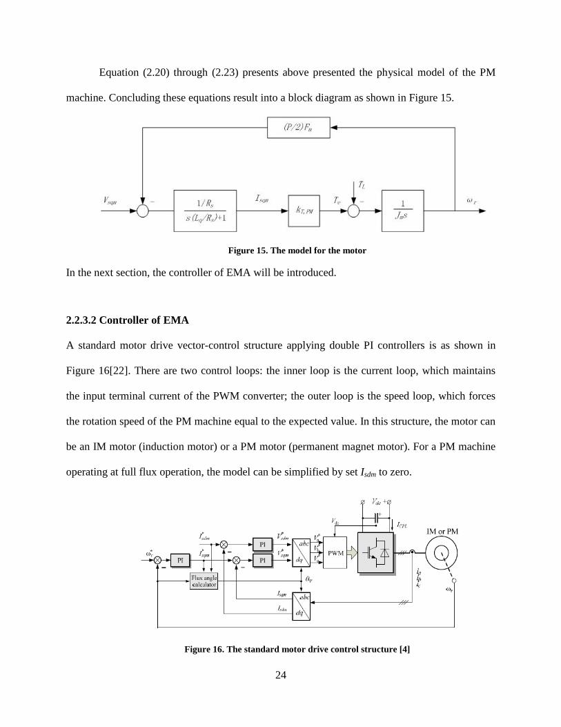
Equation (2.20) through (2.23) presents above presented the physical model of the PM

machine. Concluding these equations result into a block diagram as shown in Figure 15.

Figure 15. The model for the motor

In the next section, the controller of EMA will be introduced.

2.2.3.2 Controller of EMA

A standard motor drive vector-control structure applying double PI controllers is as shown in

Figure 16[22]. There are two control loops: the inner loop is the current loop, which maintains

the input terminal current of the PWM converter; the outer loop is the speed loop, which forces

the rotation speed of the PM machine equal to the expected value. In this structure, the motor can

be an IM motor (induction motor) or a PM motor (permanent magnet motor). For a PM machine

operating at full flux operation, the model can be simplified by set Isdm to zero.

Figure 16. The standard motor drive control structure [4]

25

Without considering the d-axis current, the control structure can be simplified as only the

q-axis current loop is analysed. The simplified control structure can be drawing as:

PI PI ConverterPM

machine

dq/abc

ωr* ωr

IabcIsqm

Isqm* Vsqm*

Vdc

Vsqm

Figure 17. The control structure neglecting d-axis current dynamic

The two PI controllers in the

Figure 17 are defined as:

Speed controller: 𝑘𝑃𝜔 + 𝑘𝐼𝜔𝑆

, and q-axis current controller: 𝑘𝑃𝑖 + 𝑘𝐼𝑖𝑆

.

Then the following equations describing the speed and q-current dynamic PI controllers

can be derived from the control structure:

𝑘𝑃𝜔𝑘𝐼𝜔−1𝜔�̇� + 𝑘𝐼𝜔−1𝐼�̇�𝑞𝑚∗ − 𝑘𝑃𝜔𝑘𝐼𝜔−1�̇�𝑟∗ = −𝜔𝑟 + 𝜔𝑟∗

𝑘𝑃𝐼𝑘𝐼𝑖−1𝐼�̇�𝑞𝑚 + 𝑘𝐼𝑖−1�̇�𝑠𝑞𝑚∗ − 𝑘𝑃𝑖𝑘𝐼𝑖−1𝐼�̇�𝑞𝑚∗ = −𝐼𝑠𝑞𝑚 + 𝐼𝑠𝑞𝑚∗ (2. 24)

The controller output signal is the q-axis reference voltage Vsqm* feeding Vsqm

* into the converter

and through a PWM process result in the voltage Vsqm. This PWM process should be derived

accurately in order to model the dynamic impact of DC-link voltage changes, especially on the

DC link current. Figure 18 illustrates the non-linear block structure for the PWM process.

26

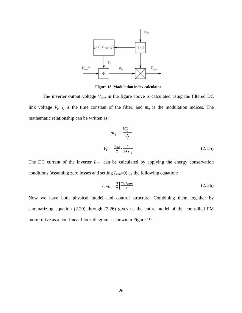
Figure 18. Modulation index calculator

The inverter output voltage Vsqm in the figure above is calculated using the filtered DC

link voltage Vf. τf is the time constant of the filter, and mq is the modulation indices. The

mathematic relationship can be written as:

𝑚𝑞 =𝑉𝑠𝑞𝑚∗

𝑉𝑓

𝑉𝑓 = 𝑉𝑑𝑐2∙ 11+𝑠𝜏𝑓

(2. 25)

The DC current of the inverter ICPL can be calculated by applying the energy conservation

conditions (assuming zero losses and setting Isdm=0) as the following equation:

𝐼𝐶𝑃𝐿 = 32�𝑚𝑞𝐼𝑠𝑞𝑚

2� (2. 26)

Now we have both physical model and control structure. Combining them together by

summarizing equation (2.20) through (2.26) gives us the entire model of the controlled PM

motor drive as a non-linear block diagram as shown in Figure 19.

27

Figure 19. Block diagram of the non-linear EMA model for PM machine [4]

2.2.4 Ideal CPL load

When a motor is tightly controlled, it behaves as a constant power load. In other words, if the

angular speed and the torque of the motor remain constant, the power of the motor will stay as a

constant:

𝑃 = 𝑇 × 𝛺 = 𝐼 × 𝑉 (2. 27)

Let us consider about the following circuit:

Figure 20. DC source feeding a CPL load through a low-pass filter

28

In Figure 20, due to the constant power, a small increment of current ICPL will cause a small

decrement of voltage VCPL, and vise versa. Mathematically:

𝑑𝑉𝐶𝑃𝐿𝑑𝐼𝐶𝑃𝐿

< 0 = −𝑅𝑐𝑝𝑙 (2. 28)

That is to say that a CPL causes a negative resistance.

A negative resistance will degrade the system stability. The dynamic model of Figure 20

can be written as:

𝑉𝐶𝑃𝐿 =𝑉𝑑𝑐 ∙ �

1𝑠𝐶 ∥ −𝑅𝑐𝑝𝑙�

𝑠𝐿 + 1𝑠𝐶 ∥ −𝑅𝑐𝑝𝑙

𝑉𝐶𝑃𝐿𝑉𝑑𝑐

= 𝑅𝑐𝑝𝑙𝑠2𝐶𝐿𝑅𝑐𝑝𝑙−𝑠𝐿

(2. 29)

It is clearly showing that the transfer function above has non-negative poles, which

means the system could not be stable without a controller. The double PI controllers have already

been introduced in the section 2.2.2.2, and they not only keep the output voltage equal to the

reference, but also remain the DC current at a proper level.

An ideal CPL load can be modeled as a voltage-dependent current source:

Figure 21. Ideal CPL load represented by a current source

In which Vout is the voltage across the DC-link capacitor and PCPL is the power level of CPL.

29

2.2.5 Combined model of the whole studied system

So far we have analysed every part of the studied system in detail, now we can combine them

together to get the mathematic model for the whole studied MEA power system.

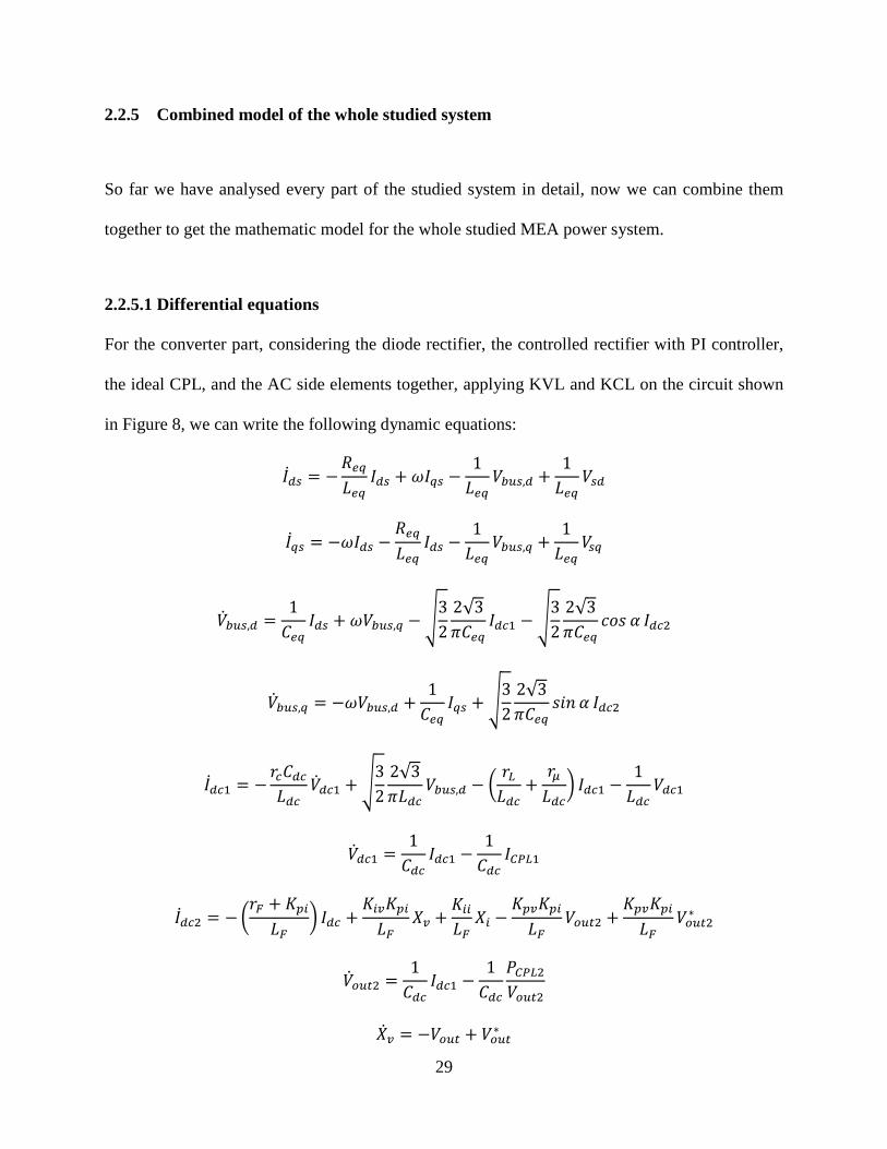
2.2.5.1 Differential equations

For the converter part, considering the diode rectifier, the controlled rectifier with PI controller,

the ideal CPL, and the AC side elements together, applying KVL and KCL on the circuit shown

in Figure 8, we can write the following dynamic equations:

𝐼�̇�𝑠 = −𝑅𝑒𝑞𝐿𝑒𝑞

𝐼𝑑𝑠 + 𝜔𝐼𝑞𝑠 −1𝐿𝑒𝑞

𝑉𝑏𝑢𝑠,𝑑 +1𝐿𝑒𝑞

𝑉𝑠𝑑

𝐼�̇�𝑠 = −𝜔𝐼𝑑𝑠 −𝑅𝑒𝑞𝐿𝑒𝑞

𝐼𝑑𝑠 −1𝐿𝑒𝑞

𝑉𝑏𝑢𝑠,𝑞 +1𝐿𝑒𝑞

𝑉𝑠𝑞

�̇�𝑏𝑢𝑠,𝑑 =1𝐶𝑒𝑞

𝐼𝑑𝑠 + 𝜔𝑉𝑏𝑢𝑠,𝑞 − �32

2√3𝜋𝐶𝑒𝑞

𝐼𝑑𝑐1 − �32

2√3𝜋𝐶𝑒𝑞

𝑐𝑜𝑠 𝛼 𝐼𝑑𝑐2

�̇�𝑏𝑢𝑠,𝑞 = −𝜔𝑉𝑏𝑢𝑠,𝑑 +1𝐶𝑒𝑞

𝐼𝑞𝑠 + �32

2√3𝜋𝐶𝑒𝑞

𝑠𝑖𝑛 𝛼 𝐼𝑑𝑐2

𝐼�̇�𝑐1 = −𝑟𝑐𝐶𝑑𝑐𝐿𝑑𝑐

�̇�𝑑𝑐1 + �32

2√3𝜋𝐿𝑑𝑐

𝑉𝑏𝑢𝑠,𝑑 − �𝑟𝐿𝐿𝑑𝑐

+𝑟𝜇𝐿𝑑𝑐

� 𝐼𝑑𝑐1 −1𝐿𝑑𝑐

𝑉𝑑𝑐1

�̇�𝑑𝑐1 =1𝐶𝑑𝑐

𝐼𝑑𝑐1 −1𝐶𝑑𝑐

𝐼𝐶𝑃𝐿1

𝐼�̇�𝑐2 = −�𝑟𝐹 + 𝐾𝑝𝑖𝐿𝐹

� 𝐼𝑑𝑐 +𝐾𝑖𝑣𝐾𝑝𝑖𝐿𝐹

𝑋𝑣 +𝐾𝑖𝑖𝐿𝐹

𝑋𝑖 −𝐾𝑝𝑣𝐾𝑝𝑖𝐿𝐹

𝑉𝑜𝑢𝑡2 +𝐾𝑝𝑣𝐾𝑝𝑖𝐿𝐹

𝑉𝑜𝑢𝑡2∗

�̇�𝑜𝑢𝑡2 =1𝐶𝑑𝑐

𝐼𝑑𝑐1 −1𝐶𝑑𝑐

𝑃𝐶𝑃𝐿2𝑉𝑜𝑢𝑡2

�̇�𝑣 = −𝑉𝑜𝑢𝑡 + 𝑉𝑜𝑢𝑡∗

30

�̇�𝑖 = −𝐼𝑑𝑐2 − 𝐾𝑝𝑣𝑉𝑜𝑢𝑡 + 𝐾𝑖𝑣𝑋𝑣 + 𝐾𝑝𝑣𝑉𝑜𝑢𝑡∗ (2. 30)

Note that both the equivalent circuit of diode rectifier and the controlled rectifier in the rotating

d-q frame are fixed on the phase of Vbus. This makes the d-axis input current of the diode rectifier

equals to �322√3π𝐼𝑑𝑐1, and q-axis input current equals to 0; and makes the d-axis input current of

the controlled rectifier equals to �322√3π

cos𝛼 𝐼𝑑𝑐2 , and q-axis input current equals to

�322√3π

sin𝛼 𝐼𝑑𝑐2. Therefore the total input current in d-q frame Iin,d and Iin,q are equal to the sum

of the diode rectifier input terminal current and controlled rectifier input terminal current in d-q

frame correspondingly, as shown in the 3rd and 4th equation in (2.30). The last two equations of

(2.30) describe the double PI control structure of the controlled rectifier in Figure 14. ICPL1 in the

above equation corresponds to the DC current of EMA model calculated in (2.26), and PCPL2

corresponds to the power level of the ideal CPL load driving by the controlled rectifier.

For the EMA part, following equations summaries the dynamics of the PWM controlled

PM motor:

𝐽𝑚�̇�𝑟 = 𝐾𝑇𝐼𝑠𝑞𝑚 − 𝑇𝐿

𝐼�̇�𝑞𝑚 = −𝑃𝐹𝑚𝜔𝑟

2𝐿𝑞−𝑅𝑠𝑚𝐿𝑞

𝐼𝑠𝑞𝑚 +𝑉𝑠𝑞𝑚𝐿𝑞

𝜏𝑓�̇�𝑓 = −𝑉𝑓 +𝑉𝑑𝑐2

𝐾𝑃𝑖𝑚𝐾𝐼𝑖𝑚

𝐼�̇�𝑞𝑚 +�̇�𝑠𝑞𝑚∗

𝐾𝐼𝑖𝑚−𝐾𝑃𝑖𝑚𝐼�̇�𝑞𝑚∗

𝐾𝐼𝑖𝑚= −𝐼𝑠𝑞𝑚 + 𝐼𝑠𝑞𝑚∗

𝐾𝑃𝜔𝐾𝐼𝜔

�̇�𝑟 +𝐼�̇�𝑞𝑚∗

𝐾𝐼𝜔−𝐾𝑃𝜔�̇�𝑟∗

𝐾𝐼𝜔= −𝜔𝑟 + 𝜔𝑟∗

(2. 31)

31

The first three equations describe the physical model of EMA, which derived in section 2.2.3.1.

The last two equations describe the vector controller of EMA, which derived in section 2.2.3.2.

2.2.5.2 Linearization and the state space model

For stability analysis, the set of equations (2.30)-(2.31) is linearized using the first order terms of

the Taylor expansion. The general state space equations have the representation as the following

matrix form:

δ�̇� = 𝐀(x0, u0)δ𝐱 + 𝐁(x0, u0)δ𝐮

δ𝐲 = 𝐂(x0, u0)δ𝐱 + 𝐃(x0, u0)δ𝐮 (2. 32)

where the state variables are:

𝐱 = [Ids, Iqs, Vbus,d, Vbus,q, Idc1, Vdc1,ωr, Isqm, Vf, Vsqm∗ , Isqm∗ , Idc2, Vout2, Xv, Xi]T (2. 33)

The matrix x has the dimension of 15×1.

The input matrix is written as:

𝐮 = [ωr∗, TL, Vout2∗ ]T (2. 34)

The matrix u has the dimension of 3×1.

The output matrix is written as:

𝐲 = [Vdc1, Vout2]T (2. 35)

Which has the dimension of 2×1.

The detailed matrix A, B, C, and D are given in the appendix A.

32

3.0 SIMULATION AND RESULTS

In this chapter, the simulation applying MATLAB and the simulation results are presented. It is

necessary to sort the fixed parameters at the beginning as shown in the appendix B. The result of

applying the full state feedback controller is also presented in this chapter.

3.1 STABILITY ANALYSIS

In the simulation part, due to the difficulty of calculating the equilibrium point of the EMA

model, it will only focus on the power levels of the EMA load rather than considering the

parameter changes in the EMA model, and only consider about the DC output voltage of the

controller rectifier. Now the system is simplified to a single input single output system.

The method for stability analysis in this chapter is using the eigenvalue theorem. The

eigenvalue of the system can be calculated from the matrix A(x0,u0) in (2.32) by solving the

eigenfunction:

det[λI-A]=0 (3. 1)

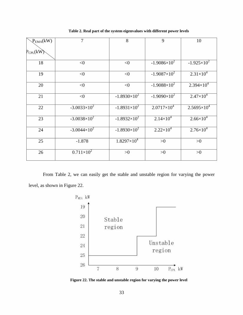
The stability region of the system can be influenced by the system parameters. Table 2

shows the real part of the dominate eigenvalues of the system corresponding to different power

levels.

33

Table 2. Real part of the system eigenvalues with different power levels

PEMA(kW)

PCPL(kW)

7 8 9 10

18 <0 <0 -1.9086×102 -1.925×102

19 <0 <0 -1.9087×102 2.31×104

20 <0 <0 -1.9088×102 2.394×104

21 <0 -1.8930×102 -1.9090×102 2.47×104

22 -3.0033×102 -1.8931×102 2.0717×104 2.5695×104

23 -3.0038×102 -1.8932×102 2.14×104 2.66×104

24 -3.0044×102 -1.8930×102 2.22×104 2.76×104

25 -1.878 1.8297×104 >0 >0

26 0.711×102 >0 >0 >0

From Table 2, we can easily get the stable and unstable region for varying the power

level, as shown in Figure 22.

Figure 22. The stable and unstable region for varying the power level

34

A critical stable case at the point PEMA=7kW, PCPL=25kW has the step response as shown

in Figure 23.

Figure 23. Step response of the system at (PEMA=7kW, PCPL=25kW)

An unstable case at the point PEMA=6kW, PCPL=26kW has the step response as shown in Figure

24.

35

Figure 24. Step response of the system at (PEMA=6kW, PCPL=26kW)

From the stable region in the Figure 22, it can be seen that increasing CPL load can significantly

degrade the system stability.

The frequency of the system can also influence the system stability region. Figure 25

shows the stability region of the system by fixing PCPL=23000kW.

36

Figure 25. Instability line for changing frequencies

As we can see in the Figure 25, high system frequency upgrades the system stability.

3.2 APPLYING STATE FEEDBACK CONTROLLER

The theorem of the state feedback can be described as following [24]: If (A, b) is controllable,

then by state feedback u=r-kx, the eigenvalues of A-bk can arbitrarily be assigned.

The principles for pole-placement and the procedures of k matrix calculation can be

found in any modern control theory textbook, or we can get k using MATLAB function

place/acker, therefore it is not necessary to put it in this thesis.

For the selection of feedback vector k, a classical method is to applying the linear

quadratic regulator method. MATLAB offers a function to use this method and select the optimal

coefficients k to stabilize the system.

Now let us design a state feedback controller for the case when PCPL=10kW and

PEMA=50kW. The original system has the eigenvalues of 10014, -373.37±j9.1494×107, -

37

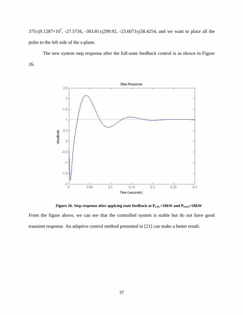
375±j9.1287×107, -27.5716, -303.81±j299.92, -23.6073±j58.4254, and we want to place all the

poles to the left side of the s-plane.

The new system step response after the full-state feedback control is as shown in Figure

26.

Figure 26. Step response after applying state feedback at PCPL=10kW and PEMA=50kW

From the figure above, we can see that the controlled system is stable but do not have good

transient response. An adaptive control method presented in [21] can make a better result.

38

4.0 CONCLUSION

This thesis deals with the modeling and stability study of a MEA power system with hybrid

converters and loads, and proposes a control design method using state feedback. DQ

transformation method is used to derive the dynamic models of the diode rectifier and the

controlled rectifier, and it is a convenient bridge to combine each subsystem. The EMA model is

represented as a PM machine drive under the standard vector-control, however the equilibrium

point is hard to evaluate and need a further study. An ideal CPL load degrades the system

stability and modeled as a voltage-dependent current source. The results are validated by

MATLAB, and the system stability region is analysed by calculating the system eigenvalues. To

improve control performance, a full-state feedback control method is developed that can

significantly increase the stability margin of MEA power system, however the transient response

of the system is not as expected and more advanced control strategy need to be implemented as

the future work.

39

APPENDIX A

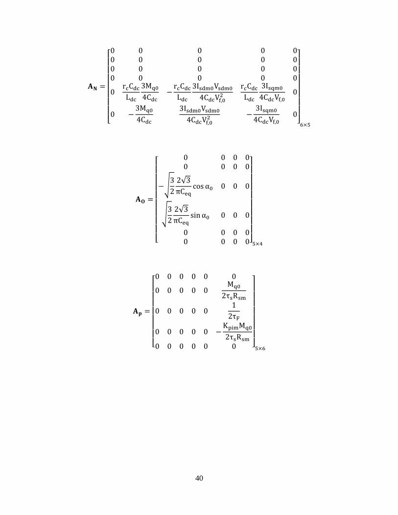
THE DETAILS OF MATRICES OF THE STATE SPACE MODEL

The detail of matrix A:

𝐀(𝐱𝟎,𝐮𝟎) = �𝐀𝐌 𝐀𝐍 𝐀𝐎𝐀𝐏 𝐀𝐐 00 0 𝐀𝐑

�

15×15

where

𝐀𝐌 =

⎣⎢⎢⎢⎢⎢⎢⎢⎢⎢⎢⎢⎢⎢⎢⎡−

Req

Leqω −

1Leq

0 0 0

−ω −Req

Leq0 −

1Leq

0 0

1Ceq

0 0 ω −�32

2√3πCeq

0

01

Ceq−ω 0 0 0

0 0 �32

2√3πLdc

0 −�rL + rµ + rC

Ldc� −

1Ldc

0 0 0 01

Cdc0

⎦⎥⎥⎥⎥⎥⎥⎥⎥⎥⎥⎥⎥⎥⎥⎤

6×6

40

𝐀𝐍 =

⎣⎢⎢⎢⎢⎢⎢⎢⎡0 0 0 0 00 0 0 0 00 0 0 0 00 0 0 0 0

0rcCdcLdc

3Mq0

4Cdc−

rcCdcLdc

3Isdm0Vsdm04CdcVf,02

rcCdcLdc

3Isqm04CdcVf,0

0

0 −3Mq0

4Cdc3Isdm0Vsdm0

4CdcVf,02−

3Isqm04CdcVf,0

0⎦⎥⎥⎥⎥⎥⎥⎥⎤

6×5

𝐀𝐎 =

⎣⎢⎢⎢⎢⎢⎢⎢⎢⎡

0 0 0 00 0 0 0

−�32

2√3πCeq

cosα0 0 0 0

�32

2√3πCeq

sinα0 0 0 0

0 0 0 00 0 0 0⎦

⎥⎥⎥⎥⎥⎥⎥⎥⎤

5×4

𝐀𝐩 =

⎣⎢⎢⎢⎢⎢⎢⎢⎡0 0 0 0 0 0

0 0 0 0 0Mq0

2τsRsm

0 0 0 0 01

2τF

0 0 0 0 0 −KpimMq0

2τsRsm0 0 0 0 0 0 ⎦

⎥⎥⎥⎥⎥⎥⎥⎤

5×6

41

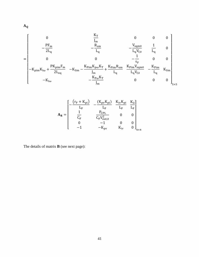
𝐀𝐐

=

⎣⎢⎢⎢⎢⎢⎢⎢⎢⎢⎢⎡ 0

KT

Jm0 0 0

−PFm2Lq

−Rsm

Lq−

Vsqm0LqVf,0

1Lq

0

0 0 −1τF

0 0

−KpimKlω +PKpimFm

2Leq−KIim −

KPimKpωKT

Jm+

KPimRsm

Lq

KPimVsqm0LqVf,0

−KPim

LqKIim

−KIω −KPωKT

Jm0 0 0

⎦⎥⎥⎥⎥⎥⎥⎥⎥⎥⎥⎤

5×5

𝐀𝐑 =

⎣⎢⎢⎢⎢⎢⎡−

�rF + Kpi�LF

−(KpvKpi)

LF

KivKpi

LFKii

LF1

CFPCPL

CFVout,02 0 0

0 −1 0 0−1 −Kpv Kiv 0 ⎦

⎥⎥⎥⎥⎥⎤

4×4

The details of matrix B (see next page):

42

𝐁(𝐱𝟎,𝐮𝟎) =

⎣⎢⎢⎢⎢⎢⎢⎢⎢⎢⎢⎢⎢⎢⎢⎢⎢⎢⎢⎡

0 0 00 0 00 0 00 0 00 0 00 0 0

0 −1

Jm0

0 0 00 0 0

KPImKIωKPImKpω

Jm0

KIωKpω

Jm0

0 0KPvKPi

LF0 0 00 0 10 0 Kpv ⎦

⎥⎥⎥⎥⎥⎥⎥⎥⎥⎥⎥⎥⎥⎥⎥⎥⎥⎥⎤

15×3

The detail of matrix C:

𝐂(𝐱𝟎,𝐮𝟎) = [0 0 0 0 0 1 0 0 0 0 0 0 1 0 0]1×15

The detail of matrix D:

𝐃(x0, u0) = [0 0 0]1×3

43

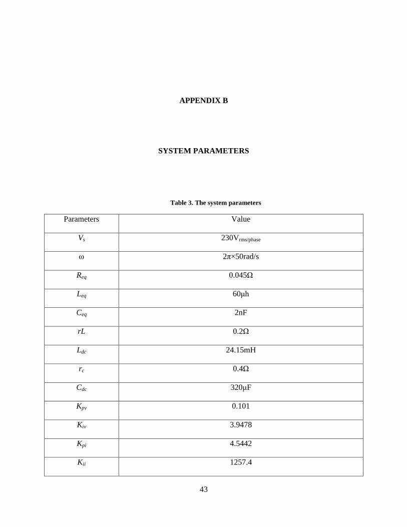
APPENDIX B

SYSTEM PARAMETERS

Table 3. The system parameters

Parameters Value

Vs 230Vrms/phase

ω 2π×50rad/s

Req 0.045Ω

Leq 60μh

Ceq 2nF

rL 0.2Ω

Ldc 24.15mH

rc 0.4Ω

Cdc 320μF

Kpv 0.101

Kiv 3.9478

Kpi 4.5442

Kii 1257.4

44

BIBLIOGRAPHY

[1] J.A.Rosero, J.A. Ortega, E. Aldabas, and L. Romeral, “Moving Towards a More Electric Aircraft”, IEEE A&E Systems Magzine, March 2007.

[2] A.Emadi, A. Khaligh, C. H. Rivetta, and G.A. Williamson, “Constant Power Loads and Negtive Impedance Instability in Automotive Systems: Definition, Modeling, Stability, and Control of Power Electronic Converters and Motor Drives,” IEEE Trans. On Vehicular Tech., vol. 55, no.4, pp. 1112-1125, July 2006.

[3] A. Emadi, B. Fahimi and M. Ehsani, “On the concept of Negtive Impedance Instability in the More Electric Aircraft Power Systems with Constant Power Loads,” Soc. Automotive Eng. J., pp.689-699, 1999

[4] Areerak, K-N, S.V. Bozhko, L. de Lillo, G.M. Asher, D.W.P. Thomas, A. Watson, T. Wu, “The Stability Analysis of AC-DC Systems Including Actuator Dynamics for Aircraft Power Systems,” In Proceedings of the 13th European Conference on Power Electronics and Applications, (EPE 2009), Barcelona, Spain, Sept. pp.8-10,2009

[5] J. Mahdavi, A. Emadi, M.D. Bellar and M. Ehsani, “Analysis of Power Electronic Converters Using the Generalized State-Space Averaging Approach,” IEEE Trans. On circuit and Systems, vol. 44, pp.767-770, August 1997.

[6] Emadi, A., “Modeling and Analysis of Multi-converter DC Power Electronic Systems Using the Generalized State-space Averaging Method,” IEEE Trans. On Indus. Elect., vol. 51. No. 3, pp.661-668, June 2004.

[7] Emadi, A., “Modeling of Power Electronic Loads in AC Distribution Systems Using the generalized State-space Averaging Method,” IEEE Transactions on Indus. Elect., vol. 51. No. 5, pp.992-1000, Oct. 2004.

[8] Han, L., Wang, J. and Howe, D., “State-space Average Modeling of 6 and 12 pulse Diode Rectifiers,” In Proceedings of the 12th European Conference on Power Electronics and Applications, Aalborg, Denmark, Sept. 2007

[9] Glover, S. F., “Modeling and Stability Analysis of Power Electronics Based Systems,” Ph.D. dissertation, Purdue University, West Lafayette, IN, May 2003.

45

[10] Rim, C. T., Hu, D. Y., and Cho, G. H. “Transformers as Equivalent Circuits for Switches: General Proofs and DQ Transformation- based Analyses,” IEEE Transactions on Industry Applications, vol. 26, No. 4, pp.777-785, July/Aug. 1990.

[11] Areerak, K-N, S.V. Bozhko, G.M.Asher, and D. W.P. Thomas, “Stability analysis and modeling of AC-DC System with Mixed Load Using DQ Transformation Method.” In Proceedings of the IEEE International Symposium on Industrial Electronics (ISIE08)., Cambridge, UK, vol.29, pp.19-24, June-2/July 2008

[12] Areerak, K-N, S.V. Bozhko, G.M.Asher, L. De Lillo and D. W.P. Thomas, “Stability Study for a Hybrid AC-DC More-Electric Aircraft Power System”, IEEE Transactions on Aerospace and Electronic Systems, vol.48, No.1 Jan. 2012

[13] “More Open Electrical Technologies European FP6 Project: http://www.moetproject.eu.

[14] T.Wu, S. Bozhko, G.Asher, P. Wheeler, and D. Thomas, “Fast Reduced Functional Models of Eletromechanical Actuators for More-Electric Aircraft Power System Study”, SAE International Conference 2008, Seattle, USA, November 2008.

[15] Kundur P. “Power system stability and control [M]”. New York: McGraw-hill, 1994.

[16] Temesgen Mulugeta Haileselassie, “Control of Multi-terminal VSC-HVDC Systems”, Master of Science in Energy and Environment, Department of Electrical Power Engineering, Norwegian University of Science and Technology, Trondheim, 2008.

[17] N.Mohan, T.M. Underland, and W.P. Robbins, Power Electronics: Converters, Applications, and Design, John Wiley & son, USA, 2003, pp. 106-108.

[18] M. Sakui, H. Fujita, and M. Shioya, “A Method for Calculating Harmonic Currents of a Three-Phase Bridge Uncontrolled Rectifier with DC Filter,” IEEE Trans. On Indus. Elect., vol. 36, no.3 pp. 434-440, August 1989.

[19] Koson Chaijaroenudomrung, Kongpan Areeak, Kongpol Areeak, “The Stability Study of AC-DC Power System with Controlled Rectifier Including Effect of Voltage Control”, European Journal of Scientific Research, ISSN 1450-216X Vol.62 No.4 (2011), pp. 463-480, EuroJorunals Publishing, Inc. 2011

[20] Chaijaroenudomrung, K., K-N., Areerak, and K-L., Areerak, 2010. “Modeling of Three-phase Controlled Rectifier using a DQ method”, 2010 International Conference on Advances in Energy Engineering (ICAEE 2010), Beijing, China: June 19-20, pp.56-59.

[21] Koson Chaijarurnudomrung, Kongpan Areerak, Kongpol Areerak, and Umaporn Kwannetr, “Optimal Controller Design of Three-Phase Controlled Rectifier Using Artificial Intelligence Techniques”, ECTI Transactions on Electrical Eng., Electronics, and Communications, Vol. 10, No.1 Feb. 2012

[22] B. K. Bose: Modern Power Electronics and AC Drives, Prentice Hall, 2002

46

[23] K-N Areerak, S. V. Bozhko, G.M. Asher, and D. W. P. Thomas, “DQ-Transformation Approach for Modelling and Stability Analysis of AC-DC Power System with Controlled PWM Rectifier and Constant Power Loads” In Proceedings of the 13 th International Power Electronics and Motion Control Conference (EPE-PEMC 2008), pp.2070-2077 Poznan, Poland, Sept. 1-3, 2008,.

[24] C.-T. Chen. Linear System Theory and Design, 3rd Edition, Oxford University Press, 1999.