ssc-368 probability-based ship design ... probability-based ship design procedures: a demonstration....
TRANSCRIPT

SSC-368
PROBABILITY-BASED SHIPDESIGN PROCEDURES:
A DEMONSTRATION
.
This document has been approvedfor public releaseand sale; its
distribution is unkn.ited
SHIP STRUCTURE COMMITTEE
1993

,-.–.._,<._ ,.,-..
,,‘1

SHIP STRUCTURECOMMllTE~
The SHIPSTRUCTURECOMMllTEE isconstituted to prosecutea researchprogramto improvethehullstructuresofshipsandothermarinestructuresbyanextensionofknowledgepertainingtodesign,materials,andmethodsofconstruction.
RADMA E. Henn,USCG(Chairman)Chief,OffrceofMarineSafety,SecurityandEnvironmentalProtection
U.S. CoastGuard
Mr.ThomasH, Peirce Mr.H.T. Hailer Dr.DonaldIiuMarineResearchandDevelopment ,+sociateAdministratorforShip-
CoordinatorSeniorVicePresident
buil$ngandShipOperations AmericanBureauofShippingTransportationDevelopmentCenter Marit]meAdministrationTransportCanada
Mr.AlexanderMalakhoff Mr.ThomasW.Allen Mr.WarrenNethercoteDirector,StructuralIntegrity EngineeringOfticer(N7)Subgroup(SEA05P)
Head,Hydronauti=SectionMilitarySealiftCommand
NavalSeaSystemsCommandDefenceResearchEstablishment-Atlantic
FXFCUTlVFi31RFCTOR CONTRACTINGOFFICFRTFCHNICAI RFPRFS~NTATlVE
CDRStephenE. Sharpe,USCGShi StructureComm”tiee
Mr.kWliamJ, SiekierkaSEA05P4
U,! CoastGuard NavalSea SystemsCommand
SHIP STRUCTURESUBCOMMllTEE
TheSHIPSTRUCTURESUBCOMMllTEEactsfortheShipStructureCommitteeontechnicalmattersbyprovidingtechnicalcoordinationfordeterminatingthegoalsandobjectivesoftheprogramandbyevaluatingandinterpretingtheresultsintermsofstructuraldesign,construction,andoperation.
AMERICANBUREAUOF SHIPPING NAVALSFA SYSTFMS COMMAND TRANSPORTCANADA
Mr.StephenG.Arntson(Chairman) Mr.W. ThomasPackardMr.JohnF. ConIon
Mr.JohnGrinsteadMr.CharlesL Null
Mr.PhillipG. RynnMr. IanBayly
Mr.EdwardKadalaMr.WilliamHanzelek
Mr.DavidL.StocksMr.AHenH. Engle Mr.Peter17monin
MILITARYSEALIFTCOMMAND MARITIMFADJvflNISTRATION U. S. COASTGUARD
Mr.RobertE.VanJones Mr.FrederickSeibold CAPTT. E.ThompsonMr.RickardA Anderson Mr.NormanO. HammerMr.MichaelW. Touma
CAPTW. E. Colburn,Jr.Mr.ChaoH. Lin
Mr.JeffreyE. BeachMr.RubinScheinberg
Dr.WalterM. Maclean Mr.H. PaulCojeen
DEFE~NTIC
Dr.NeilPegg
IAISONMFMRFRs
U, S. COASTGUARDACADFMY
LCDRBruceR. Mustain
U. S. MERCHANTMARINEACADEMY
Dr.C. B. Kim
U. S. NAVALACADEMY
~s -Dr.RobertSielski
NATIONALACADEMY OF SCIENCES-~s
Mr.PeterM. Palermo

MemberAgencies:
United States Coast GuardNaval Sea Systems Command
Maritime AdministrationAmerican Bureau of Sh@ping
Military Sealift CommandTranspoti Canada
ShipStructure
CommitteeAn InteragencyAdvisoryCommittee
August 13, 1993
AddressCorrespondenceto:
ExecutiveDirectorShipStructureCommitteeU.S. CoastGuard(G-Ml/R)2100SecondStreet,S.W.Washington,D.C. 20593-0001PH:(202)267-0003FAX:(202)267-4677
SSC-368SR-1330
PROBABILITY BASED SHIP DESIGN PROCEDURES:A DEMONSTRATION
This report provides a demonstration on the use of probabilitybased ship structural design and compares its benefits versusthose of traditional methods. Relative to other traditionalapproaches, reliability methods hold the promise of a betterunderstanding of engineering design. It is anticipated that inthe future the use of these methods will result in a balancebetween reduced structure weight and life cycle cost andincreased reliability. Other fields of engineering such civilengineering and offshore structures have lead the way indemonstrating the benefit of these methods.
This report gives two basic demonstrations which illustrate thedevelopment and calibration of design criteria for uniform safetyover a wide range of basic parameters involved in design andapplies the state of the art reliability techniques to hullgirder safety analysis of existing vessels. In doing so astandardized structural reliability terminology, limit states andload extrapolation techniques are defined for future projects.The report concludes with and evaluation of benefits anddrawbacks of using the method and gives recommendations forfuture research.
G.E.7&A. E. HENN
Rear Admiral, U.S. Coast GuardChairmanr Ship Structure Committee

TechnicalReportDocumentationPage
1. ReponNo. I 2 GwemmentAooassionNo. I 3, RedplenrsCatiogNo.
SSC-368 I I
PROBABILITY-BASED SHIP DESIGN (PHASE 1)A DEMONSTMTION
~1
7. Author(s) I 8. PerformingOrganizationRe~rlNo.A. Mansour, M. Lin, L. Hovem, A. Thayarnballi SR-1330
9. PerformingOrganizationNamsendAddress 10.WorkUnitNo.~RAIS)
Mansour Engineering, Inc.14 Maybeck Twin Dr. 11.ContractorGtamNo.
Berkeley, CA 94708 DTCG23-9O-C-2OO1O12.SponsoringAgenq’NameandAddress 13.TYoeofRanmtandParlodCovered
Ship Structure Committee-.
U.S. Coast Guard (G-M) Final Report
2100 Second Street, SW 14. SponsoringAgerqCoda
Washington, D.C. 20593 G-M15.Supplemen~Notes
I Sponsored by the Ship Structure Committee and its Member Agencies I16. Abstraot
The report provides a demonstration on the use of probability based ship structural design methodsand enumerates the benefits in comparison to traditional methods. Two basic demonstrations areprovided. The fist illustrates the development and calibration of design criteria that produce uniformsafety over a wide range of basic parameters involved in design. The second applies state of the artreliability techniques to detemine safety levels of existing vessels, tsking into considerationuncertainties in loads, strength and calculation procedures. In addition, structural reliabilityterminology, limit states and load extrapolation techniques pertinent to ships are defined anddescribed.
Available from:Probability National Technical Information ServiceStructural ReliabilityShip Design
U.S. Department of CommerceSprin@eld, VA 22151
19. SecurilyClassif.(ofthisreprt) I 20. SW@ GISSslf.(ofthispage) 21. No. of Paaes I 22. Price
I Unclassified I Unclassified I 111 +-App. I II I I I
FormDOTF 1700.7 (B-7.2)J
Reproduction of completed page authorized
3
______ ________ _____ ____
METRICCONVERSIONFACTORS
Approxi6nstc Convm40rks to Metric Measures Approrimmtt Conversions from Metric MoasuIes
Whan YOM Know Mfllti#lr hf
LENGTH
miilinwters 0.04cantimmtem 0.4matews 3.3meters 1.1
kihmmt~s 0.6
AREA
zquafc cenfiwietws 0.16
aquam mmwn 1.2squwa ki Iometera 0.4rlactmresIIo,ooo!+ 2.s
MASS ~wciflht]
la Find
inches
inchm
leer
~arda
miles
aqwme Inclms
Squavm Vmds
aquem miles
screa
wncea
pwtmda
short tons
fluid wncoa
pinra
qunrts
gallons
cubbc feal
Cuwlc Vmrds
Fnhrad?eil
tenwrmture
Svmbot
mcm
\mmkm
C##
km’
ha
To Find S~mbd
lEHGTH
in
fr
@
mi
inches
Ieet
wzta
“2.5
300.91.6
centimtwa
cenl irwwrs
malers
kitmmatms
cmcmmkm
.2~z
n?
kmz
hm
akg
t
ml
ml
ml
I
I
I
I~3
~3
“c
mi Ias
AtlEA
in2f!’yr?miz
squm4 hlcfmm 6.5
Cqumm feet 0.0s,qUmymds 0.89wW6mil*s 2.sScm m 0.4
squara cenlimelera
squar. mews
Muava matera
heclama
MASS (weight]
wncea 28
pmda 0.45short [mm 0.9
120W lb)
VOLUME
arms01
lb
9kg
t
or
lbglmml 0.035kilqm!ns 2.2
tcmnea 11000 kg] *.1
VOLUME
milliliters 0.03Iimrs 2.1
liters 1.06
liters 0.26cubic nmara 35
cubic meler~ 1.3
TEMPERATURE [wmet]
Celsius 9/5 Ithen
f! 02
Pqt
gal
662
Vdz
m.aapnma 5
Iabl.apwns 15
fIuid ouncma 30cvpa 0,24
pints 0.47quarts 0.95Omllms 3,8cubicfeet 0.03cubicVafda O.m
TEMPERATURE (axsct~
milliliters
milliliter
mi!li litem
lilers
liters
lilets
I item
cubic melera
cubic mews
“F
‘F Fafwanhail 5/9 Iaftar
mmparalure subtract ing
321
Celsiusten-pmature “F
‘F 32 90.6 262
-40 0 40 aol,, ,1, :i{l, it, t~
!20 160 200t’; 1 1 1 4 , , , * # 1 *
I 1 I-:: -20 0 20 40 60 ‘ 00 IOD
37 ‘JC- ! m : 2.54 Enacll y!. F<. other ● xxl co.vers~.?m and mm del. aled MtIles. see NBS h!E.c. P$vbl.2W3.
Unds d Weights and. Measures. Pr,ce S2.25. SD CaIalcm No. C! 3.! 0286.
1 1

TABLE OF CONTENTS
1. Introduction, Scope and Objectives
PART 1- Demonstration of Probahilitv-Based Rule Calibration
2. Preliminary Assessment of Reliability Levels Implied in ABS Rules
2.1 Limit State Formulation
2.2 General Characteristics of “ABS Ships”
2.3 Strength Considerations of “ABS Ships”
2.3.1 Section Modulus
2.3.2 Yield Stress
2.4 Loads Applied to “ABS Ships”
2.4.1 Stil[water Bending Moment
2.4.2 Wave Bending Moment
2.4.3 Comments on the Ratio of Wave Bending Moment to Stillwuter
Bending Moment Given by ABS Rules
2.5 Safety Indices and Tim-get Reliability
2.5.1 Reliability Analysis -- First ond Second Order
2.6 Comments on ABS Rules Regarding Ship Section Modulus Calculation
3. Calibration Procedure
3.1 Procedure of Calculating Pnrtitil Sufety Factors for “ABS Ships”
3.2 Redesign of “ABS Ships” and Resulting Safety Indices
3.3 Benefits ot’the Calibrtition
1
5
5
6
6
7
7
8
10
11
12
14
14
17
25
25
26
29
PART 2- Demonstration of Prohtibilitv-Bilsed Hull Girder Stifetv Analvsis
4. Development of’Limit States for an Example Ship 31
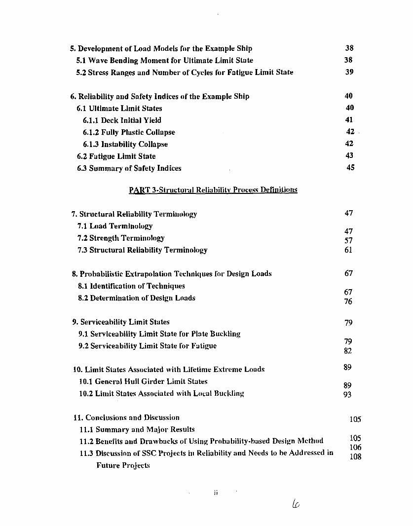
5. Development of Load Models for the Example Ship
5.1 Wave Bending Moment for Ultimate Limit State
5.2 Stress Ranges and Number of Cycles for Fatigue Limit State
6. Reliability and Safety Indices of the Example Ship
6.1 Ultimate Limit States
6.1.1 Deck Initial Yield
6.1.2 Fully Plastic Collapse
6.1.3 Instability Collapse
6.2 Fatigue Limit State
6.3 Summary of Safety Indices
38
38
39
40
40
41
42
42
43
45
PART 3-Structuriil Relitihilitv Process Definitions
7. Structural Reliability Terminology 47
7.1 Load Terminology47
7.2 Strength Terminology 577.3 Structural Reliability Terminology 61
S. Probabilistic Extrapolation Techniques fm- Design Loads 67
8.1 Identification of Techniques
8.2 Determination of Design Loads6776
9. Serviceability Limit States 79
9.1 Serviceability Limit State for Plate Buckling
9.2 Serviceability Limit State for Futigue7982
10. Limit S&~tesAssncitited with Lifetime Extreme Lotids 89
10.1 Generiil Hull Girder Limit Sttites 8910,2 Limit States Assocititwl with Loctil Buckling 93
11. Conclusions and Discussion 105
11.1 Summary and Major Results
11.2 Benefits and Drawback of Using Prohtihility.btised Design Method 105
11.3 Discussion of SSC Pro,jects in Reliability and Needs to be Addressed in106108
Future Pro,jects
ii
b

12. References110
APPENDICES
1. M~w,Mw, Mw/M~wand SM of “ABS Ships”2. Means and Standard Devi~}ticmsof M5W,MIV:lnd SM of “ABS Ships”3. Calculntions of Plastic Momtint Cripwity, Criticnl Buckling Stresses nnd Effective
Section Modulus4. C~lcuIations of Compressive Strength Fnctm-nnd the Hull Girder lnst[lhi!ity Collapse.
Moment5. Calculations of the RMS Values of the Wnve Bending Moment for the Example Ship6. Fatigue Reliability Calculations7. Typical Input/Output File.of CALREL
...Ill

Nomenclature
Shipbreadthblosckcoe5cicntshiplength
constantsdctcrmincdfromS-NcuwestillwaterIxndingmomenttotalbeudingmomentultimatemomentcapacitywavebendingmomentnumhr of waveIxndingmomentpeaksprobabilityof failuresectionmoduluselasticsectionmoduluseffectivesectionmodulusplasticsectionmodulusmodeluncertaintyassociatedwiththevariabk“i”safetyindexpartialsafetyfactortaaociatedwitha loadvariable“i”
damageindexstressrangemeanof thevariable“i”standarddeviationofvariable“i”criticalstressyieldstrengthsewicclifeof theshippartialsafetyfactorassociatedwith a resistancevariabk “i”stressparameter
Note: othersymbols are defined whereused
iv

1. Introduction, Scope and Objectives
This report, titled “Probability Based Ship Design Procedures - a Demonstration”, is
the second in the series of projects undertaken by the Ship Structure Committee in the
thrust area of reliability based ship design. The fwst was the development of a
comprehensive primer to structural reliability theory as applied to ships and marine
structures, Ref. 6. The work in this project assumes that the reader is familiar with the
various concepts and applications discussed in Ref. 6, “An Introduction to Structural
Reliability Theo@’, SSC Report 351.
The immediate objective of this project is to provide a demonstration of the use of
probability-based ship design methods and to compare the results with ~ditional design
methods. Based on the results of the demons~tion, the following conclusions and
information are provided:
L The benefits and drawbacks of the use of probability-based design methods compared
to the traditional methods
2. The additional information necessary to conduct probability-based ship designs
3. A summary of the proposed probability-based method showing how it can be applied
to generate new designs of uniform safety and how it can be used to assess the safety
of an existing design
4. A discussion of the current and future SSC projects in reliability and loads.
Two basic demonstrations are provided in this report (Part 1 and Part 2) together with
reliability process definitions (Rut 3). These are summarized as follows:
1. Probability-based design procedure -- code calibration:
The objective of this part is to provide an illustration of how probability-based
methods can be used to develop and calibrate a code (or design criteria) in order to
produce designs with uniform safety over a wide range of the basic parameters involved
in the design. For this purpose, ABS primary hull girder longitudinal strength criterion is
considered. A formulation for the minimum required section modulus that satisfies this
1

requirement (uniform safety) is develope& A demonstration is made of how partial
safety factors are determined, calibrated and used in new designs that have uniform
safety.
2. Probability-based ship safety analysis:
The objective of this part is to provide an illustration of how to apply state-of-the-art
reliability techniques in order to det.enrine the safety level of an existing ship or an
existing design, i.e., to develop the ship safety indices taking into considemtion the
uncertainties associated with the environment loads, materials and analytical models.
For this purpose a tanker was selected in consultation with the Project Technical
Committee (PTC) for use in an example to illustrate the safety assessment procedure.
Several limit states were formulated, namely ultimate, sewiceability, and fatigue limit
states, and applied to the tanker. The loads corresponding to these limit states were
developed and a safety index was calculated for each limit state using both fwst and
second order reliability methods.,
3. Structural reliability process clefmitions:
An extension of the work of this project (SR-1330) was approved by the PTC.
The additional work is described in the following tasks:
(a) Definition of terminology associated with structural reliability of ships and offshore
structures. This includes terminology related to loads, strength and structural
reliability.
(b) Identification and description of appropriate ultimate limit states associated with
lifetime extreme design loads. These include global (hull girder) initial yield, fully
plastic and collapse limit states, and local ones related to column, beam/column and
torsional/flexural buckling of longitudinal, and grillage buckling of longitudinal
together with transverse beams.
(c) Identification and description of serviceability limit states associated with plate
buckling and fatigue.
(d) A review of probabilistic extrapolation techniques for lifetime extreme loads..
2

A NOTE ON NOTATION
A distinction needs to be made between random variables and their characteristic or
nominal values, although this may often be evident from the context. In this repo~u
where necessary, random vtiables are denoted with a ‘tilde’ on the top, e.g. 6Y is a
random variable, while Oyis a nominal or characteristic value.
3
4J?)

2. Preliminary Assessment of Reliability Levels Implied in ABS Rules
As a demonstration of a probability-based calibration procedure of a code, the safety
level implied in ABS Rules for hull girder longitudinal strength is determined by
calculating the reliability indices (~s) for 300 ships designed acconi.ing to the Rules.
ne mnge of safety (~nge) was then calculated as the difference between the largest
and smallest safety indices of all the designs considered. AII avemge s~ety ~dex (~av)
was also calculated. The objective of the calibration process is to determine partial safety
factors to be used in a modified fonmdation for longitudinal strength such that the
resulting safety level of all designs is approximately constant wit-ha v~ue equal to ~av
and such that the resulting safety range (~ngJ among the new designs is minimum.
The details of the calibration process is illustrated in the following sections.
2.1 Limit State Formulation
The section modulus requirements for a ship according to ABS Rules is based on a
permissible stress which k based on the yield strength of the material. For this mson,
only the initial yield limit state will be formulated which is similar to ABS minimum
section modulus requirement. Only vertical bending moment, composed of stillwater
and wave bending moments, is considered. The initial yield limit state is expressed as:
m-
(2.1)g~ =S-M*;Y-MSW-MW
d
where X is a vector of the random variables, ( S-M,;Y, fisw, and Mw ), and
SM is the section modulus amidship,
‘Yis the yield stress,
MSw is the stillwater bending moment,and
Mw is the wave bending moment.
5
These variables are taken to be random or uncertain and are assumed to be statistically
independent.

2J General Characteristics of “ABS Ships”
The general characteristics of several ships designed to the minimum requirements of
ABS Rules (including minimum section modulus requirements) will be determined
These ships will be called “ABS Ships”. Since the initial yield limit state is the only
failure mode to be considere~ and the variables in Eq. 2.1 depend only on L, L/B, and
Cb, these three parameters seine as the factors on which the reliability level depends.
They are specified as follows:
L : from 91.5m ( 300 ft ) to 366 m ( 1200 ft )
L/B : from 5.0 to 9.0
Cb : from 0.60 to 0.85
These ranges cover most ships to which ABS Rules are meant to apply. The value
without ‘tilde’indicate deterministic characteristic values.
23 Strength Considerations of “ABS Ships”
Because of variability of properties of steel and other materials used in marine
structures and because of variability in production and fabrication of their components,
the strength of identical ships will not, in general, be identical. In addition, uncertainties
associated with residual stresses arising from welding, the presence of small holes, etc.
may affect the strength of the ship. These limitations and uncertainties indicate that a
certain variability in strength or hull capacity about some mean value will result.
Additional uncertainties in the strength will arise due to uncertainties associated with
the assumptions and methods of analysis used to calculate the strength. Further
uncertainties are associated with possible numerical errors in the analysis. These errors
may accumulate in one direction or possibly tend to cancel each other. Whatever the
case, the above uncertainties have to be reflected in any reliability or failure analysis.

~.d.f.
12567
13512
14457
17292
1B237
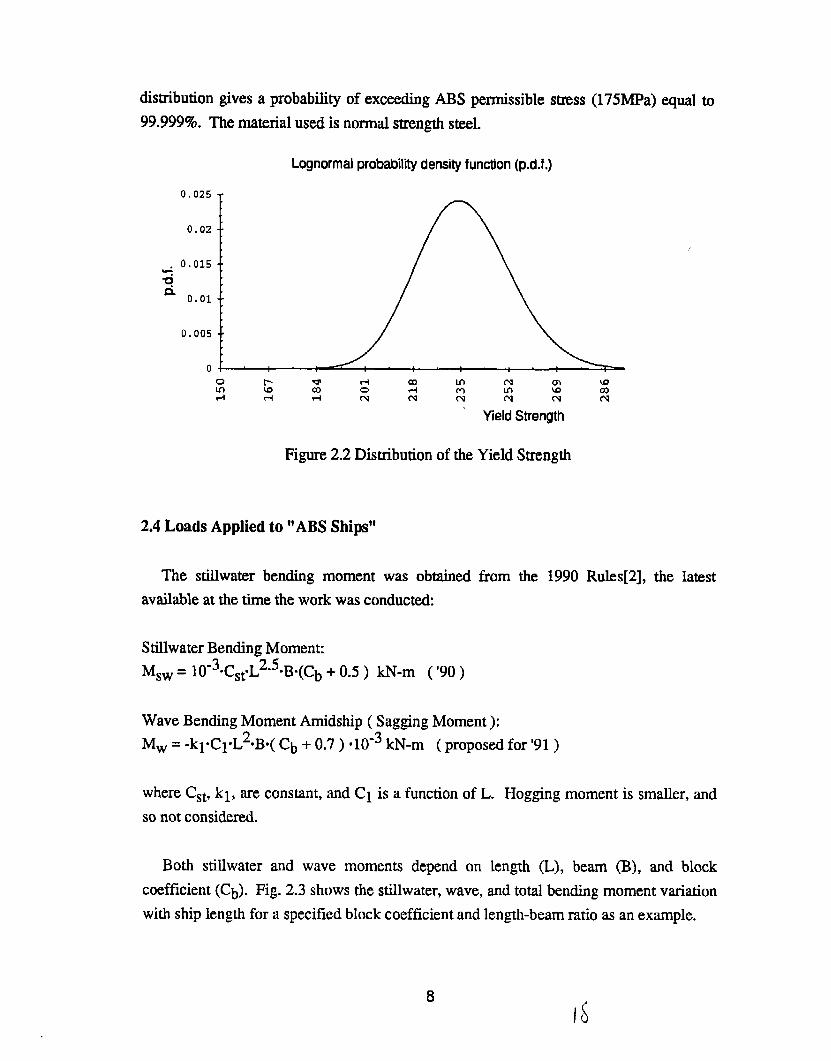
distribution gives a probability of exceeding AIM permissible stress (175MPa) equal to
99.999%J. The material used is normal strength steel.
0.025
0.02
~ 0.015
u
a 0.01
0.005
0
Lognormalprobabil”~densityfundon (p.d.f.)
YieldStrength
Figure 2.2 Distribution of the Yield Strength
2.4 Loads Applied to “ABS Ships”
The stillwater bending moment was obtained from the 1990 Rules[2], the latest
available at the time the work was conducted:
Stillwater Bending Moment
10-30Cst”L2“5.B.(Cb + ().5 ) kN-m ( ’90)MSw=
Wave Bending Moment Arnidship ( Sagging Moment):
Mw = -kl*Cl*L2*B*(Cb + 0.7 ) ●10-3 kN-m ( proposed for ’91 )
where C~t, kl, are constant, and Cl is a function of L. Hogging moment is smaller, and
so not considered.
Both stillwater and wave moments depend on length (L), beam (B), and block
coefficient (Cb). Fig. 2.3 shows the stillwater, wave, and total bending moment variation
with ship length for a specified block coefficient and length-beam ratio as an example.

3.5e+07
3M)7
2.5c+)7
2e+07
1
~..x..x MW
1.5e+07
I
,,F
,01, ply”
//’ %’
1C+07 ,d” “/,
/ .%’” y
/d’ ‘“. ,x”
5e+06 –,
a “ x’”0
.
---
0 a--.-= .1 1 1 1 1 I 1 I I 1 I 1 1 I 1 I
I1 1 1 1 1 1 z 1 1 I 1 1 1 1 1 1 T
o 100.0
Fig.2.3Total
200.0 300.0Length of Ship(m)
Bending Moment (Cb=O.6L/B=5)
fux).o
9

Appendix 1 shows the values of the stillwater moment, the wave momen~ the ratio of the
wave to stillwater moments and the minimum section modulus, all calculated according
to ABS Rules as described earlier for the selected ranges of length, length to beam ratio,
and block cmfficient.
2.4.1 Stillwater Bending Moment Distribution
According to Soares and Moan[3], the stillwater bending moment fits to a normal
distribution. In this investigation it is assumed that the value given by ABS is the
maximum value with a probability of exceedance of 5 %. The large variability in the
stillwater bending moment calls for a coefficient of variation of 4070[3] which gives the
mean value of the distribution to
PSw=0“6“%W,ABS
be:
(2.2)
where Msw,~s is the stillwater bending moment given in ABS Rules . The
distribution is shown in Fig. 2.4.
Normal Probability Density Function (p.d.f.)
o.m14
o.m12
no.-
O.-
0
Figure 2.4. Distribution of the Still Water Bending Moment
10

2.4.2 Wave Bendm~ M.
oment Distribution
If the wave loads acting on a marine structure can be represented as a stationary
Gaussian process (short-term analysis), then at least four methods are available to predict
the distribution of the maximum load. These methods are developed for application to
marine structures and are given in more detail in [4]. In this report, extreme value
distribution based on upcmssing analysis [6] is used.
The wave induced bending moment
following the distribution function[4]:
2Fw (w)= exp (-N exp (- ~ ) )
given by ABS is modeled as an extreme value
where Kw is the mean of the distribution and
number of wave bending moment peaks and k.
moment process. The value given by ABS is
(2.3)
aw is the standard deviation. N is the
is the mean square of the wave bending
assumed to be the mean value of the
distribution [6], and Table 2.1 shows how the coefficient of variation varies with N.
Choosing N to be 1000, which is equivalent to a 3 hour storm gives a coefficient of
variation of 9 %. Fig. 2.5 shows the distribution.
N C.o.v.
500 10%
1000 9%
2000 8%
Table 2.1
11

Extremevalue probabilitydensity function (p.d.f.)
0.050.0450,04
0.035. 0.03
~ 0.025Osx?
0.0150.01
0.0050120000 142500 165000 187500 210000 232500 255000
Extreme Wave Moment
Figure 2.5 Distribution of the Extreme Wave Bending Moment
Appendix 2 gives the calculated means and standard deviations of the stillwater
moment, wave moment, and the section modulus according to the distributions described
above for the selected ranges of L, L/B and Cb.
2.4.3 Comments on the Ratio of Wave to Stillwater Bending Moments
Given by ABS Rules
Inspection of the calculated values of Msw, Mw, and Mw/Msw according to ABS
Rules (Appendix 1), leads to the following conclusions:
1. M JMsw ratio does not depend on IJB. Hence, M w/Msw can be written as a
function of L and Cb only.
2. Fig. 2.6 shows the ratio Mw/Msw as a function of L for two extreme values of Cb (0.6
and 0.85). The resulting curves are more or less parallel, and each has a maximum at
L=152.5 m and a minimum at L=366.O m.
3. When L is held constant, M w/Msw ratio decreases monotonically as Cb increases.
4.& a result of the above observations, all M#fw values fall in the area bounded by

the two lines shown in Fig. 2.6. The minimum and maximum values of this ratio are
1.507 and 1.681, respectively.
1.7
1.65
~
“\\
\\
\
\
\
‘x,\\\\‘k
1.5 1 ! I I I 1 1 I 1I
1 1 1 I 1 1 1 1 1I
1 1 1 I 1 I I 1I
I 1 ,,, [ I
o 100.0 200.0 300.0 4m.oLength of Ship(m)
Fig. 2.6 MWIMSW( Cb=O.6Cb=O.8S)
as a function of length
13
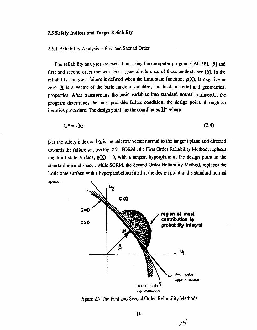
2.S Safety Indicti and Target Reliability
2.5.1 Reliability Analysis -- First and Second Gdcr
The reliability analyses arc carried out using tie computer progr~ CALREL [5] snd
f~st md second order methods. For a gene~ ~femnce of thc~ methods see [6]. In the
reliability analyses, ftilwe is defin~ when the limit s~~ function? g~, is negative or
zero. X is a vector of the bmic r~dom v~ablest i.c- 10~, ma~~~ and geometrical
properties. After transfoting the basic v~abl= in~ s~~ now wrhtes~, the
program determines the most probable failure contition, the design poin~ through an
iterative procedure. The design point has the coordinates U* where
L!*=-MI (2.4)
~ is the safety index and g is the unit row vector normal to the tangent plane and direeted
towards the failure seti see Fig. 2.7. FORM, the First Order Reliability Method, replaces
the limit state surface, gw = O, with a tangent hjpcrplane at the design point in the
standard normal space, while SORM, t.hcSecond Order Reliability Method, replaces the
limit state surface with a hypcrparaboloid fitted at the clesign point in the standard normal
space. \
m/
region of most
Contribution to
~ probability intogrol
—%
~ fust- orderapproximation
isecond-orderapproximation
Figure 2.7 The First and Second Order Reliability Methods
14
(Jq

The fwst order probability of failure, Pf, is determined from
Pf = @ (-p) (2.5)
where O is the standard nom-d distribution function. Fig. 2.8 shows the relation
between ~ and PF ‘~ is so called safety or reliability index. The higher the ~ value, the
lower the probability of failure, and the higher the safety margin between strength and
load. The relationship between ~ and Pf given in Eq. 2.5 can be determined numerically
from the properties of the standard normal distribution function [15].
CALREL was used to calculate reliability indices for the “ABS ships” covering the
entire range of L, L/B and Cb described earlier. For this purpose, the limit state equation
(2.1) and the probability distributions given in sections 2.3.1,2.3.2,2.4.1, and 2.4.2 were
used in the analysis. Based on these results the following conclusions are made:
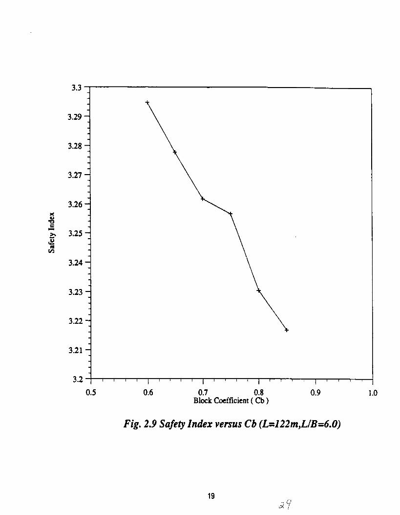
1.
2.
Holding L, L/13fixed, and varying Cb from 0.6 to 0.85
As shown in Fig 2.9, the safety index (j3)decreases monotonically as the block
coefficient increases.
Holding L, Cb freed, and varying L/B from 5.0 to 9.()
Fig 2.10 shows that ~ is almost constamt. It suggests that the impact of L/B on ~ can
be neglected.
3. Range of ~ for different L
From observations 1 and 2 above, we can conclude that within our dimensions, ~
varies between the two parallel lines shown in Fig. 2.1 l,which shows the relation
between ~ and L for the two extreme cases (Cb = 0.6 and 0.85). It is also seen
that these lines have the same pattern as M#sw lines in Fig.2.6. Fig. 2.12 and Fig.
2.13 ae plotted to illustrate the relation between ~ and Mw/M~w. The two lines
representing the boundaries of the safety indices in Figs. 2.12 and 2.13 are plotted
again in Fig. 2.14, which shows that they fall on each other. This suggests that ~ can
be treated as a function of Mw/Msw only.
4. Table 2.2 shows the upper and lower bounds of ~ for ship length varying from
152.5m to 366m. ~ ranges from 3.0236 to 3.3276 (see also Fig. 2. 14), and its average
is 3.1918.
15

L(m) Ch
91.5 0.600.85
122.0 0.600.85
152.5 0.600.85
183.0 0.600.85
213.5 0.600,85
244.0 0.600.85
274.5 0.60
0.85
305.5 0.60
0.85
353.5 0.600.85
366.0 0.60
0.85
p(L/13=5.o) p(L/B=9.o)
3.2434 3.2434
3.1635 3.1635
3.2953 3.3070
3.2165 32165
3.3276 3.3272
3.2490 3.2489
3.3200 3.3200
3.2416 3.2416
3.2933 3.2933
3.2143 3.2143
3.2148 3.2147
3.1343 3.1343
3.1992 3.1992
3.1185 3.1185
3.1774 3.1774
3.0962 3.0962
3.1389 3.1389.
3.0571 3.0571
3.1060 3.1060
3.0236 3.0236
Table 2.2 Safety Indices of ABS Ships
The safety check equation used in the calculations of ~ is given by Eq. 2.1.
16
2.6 Comments on ABS Rules Regarding Ship Section Modulus Calculation
The following conclusions can be drawn based on the results obtained in
2.5.1:
section
1. Safety implied in ABS Rules for longitudinal strength is very consistent because ~
varies within a very small range. However, the corresponding ratio of the upper and
lower values of probability of failure is 2.85. This means that some room for
improvement still exists.
2. The safety index depends only on the ratio of wave bending moment to stillwater
bending moment This makes the calibmtion procedure easier.
3. The target reliability level is set to be ~ = 3.20, which is approximately the average
value of ~ determined earlier for the “ABS Ships”.
17..--1

2Ja
aw
CA>0&
b 1
%
.
.-
fig.2.8 Probability of Failure versus Safety Index
18
3.3
3.29-
3.28-
3.27 –
3.26-
3.25-
3.24-
3.23-
3.22-
3.21 –
3.2 i 1 I 1I
1 1 I 1I
I 1 1 I1
1 1 1 I I 1 1
0.5 0.6 0.7 0.8 0.9 1.0Blwk Cmfficicnt ( Cb )
Fig. 2.9 Safety Index versus Cb (L=122m,L/B=6.0)

,.
i
3.29 –
3.28-
3.27 –
3.26-x
*ch 3.25-
~
z
3.24-
3.23-
3.22-
3.21 –
3.2 T1 11 I I 1 1 T l“’’’’’ ’’1 ’’’’’’’’’1’” “’’’ ’1 ’1 ’’’’’’’1’’” I T
4.0 5.0 6.0 7.0 8.0 9.0 10.0W@-BeamRatio( UB)
Fig. 2.10 Safety In&x versus LIB ( L=122m,Cb=0.6)
20

3.5 I
/
i
x--x--x
3.44
CIJ4.6
Cb=O.85
3.11
“\\
k -.%‘-%.,
‘.%, \
x,\\\
‘x
3.0 # I 1 1 1 I 1 r T T I T 1 1 1 1 1 i 1 I 1 6 ! i 1 I 1 I 1I
i I 1 I
o 100.0 2CHI.O 3CKL0 4M.OLength of Ship(m)
Fig. 2.11 Safety Index ( L/B=5 )
as a function of length
21.3I

3.s
3.4
3.3
3.2
3.1
3.0 I 1 I 1I
I T 1 1I
1 I I 1I
1 1 I 11
I I 1
1.5
Fig. 2.12
1.54,
Saf’tyindex
1.58 1.62 ) .66 1.7MwiWw ,
versus MWIMSW(UB=5.0,C6=0.6)
—..
22
32

3.s
3A
3.2
3.1
3.0
J
I 1 r 1I
1 T 1 II
I I I II
1 I I II
1 1 T 1
1.5 1.54 1.58 1,62 1.66 1.7
Fig. 2.13 Safety index versus Mw/Msw ( LJB=S.O,Cb=O.85)

3.5 I
CbdMs
Cb=O.6
I,J”
/
,X”,//x“
3.0 ~, , 1 1 T 1 1 I I 1I
I 1 I 1 ! 1 1 1 1I
1 1 1 i 1 I 1 1 !I
T 1 1 1
1.5 1.55 1.6Mw/Msw
Fig. 2.14 Safty index versus
1.65 1.7
MWIMSW(L/B=5.0)
3.0 Calibration Procedure
Safety factors such as those applied to yield strength and to loads are an essential part
of the design process. In the probabilistic methods, this need resulted in the introduction
of partial safety factors. The cumulative effect of those factors is such that the resulting
design will have a certain reliability level. ‘Thus, code developers and classification
societies may determine these partial safety factors that ensure that the resulting design
will have a speciiied reliability level. The method of determiningg these partial safety
factors for a given safety index is discussed in Reference[6].
The objective of this section is to detmmine partial safety factors such that when
applied to the characteristic values of stillwater moment, the wave moment and yield
strength, the resulting hull girder section moduli for all ship sizes produce constant
reliability index equal to the target reliability determined earlier, i.e., ~wget=3.2. This
value is an average value of the computered safety indices for the ABS ships and is
selected as target reliability for illustrative purposes only.
3.1 Procedure of Calculating Partial Safety Factors for “ABS Ships”
As described above, partial safety factors are used
assure a specified reliability level. For the current case,
M~W+ywMwSM = ‘Sw
$y~y
in the calibration procedure to
(3.1)
where ysw , Yw, ~d by
Mw, Oy respectively.
are the partial safety factors for the characteristic values Msw,
The following
Ships” :
procedure is used to determine the partial safety factors for the “ABS
1. By trial and error determine ~s and $ in Eq. 3.1 that gives the ~target.
2. Find out for different ratios of Mw/M sw, the value of ~ determined from FORM (or
SORM) using the ys and $ obtained in the fust step, and check if
a. the obtained ~’sare close to the target ~, and
b. the obtained ~range is smaller than that of ABS rules.
25
+0

3. If the determined ys and $ give ~s close to ~mget and ~mnge is smaller, then they
can be used in the new calibrated code, othewise make changes in them to satisfy
the two criteria a. and b. above.
32 Redesign of “ABS Ships” and Resulting Safety Indices
The procedure described above can be implemented as follows. Eq. 3.1 can be
rewritten as:
SM = yqw+mywMSw $y~y
(3.2)
where m is the ratio of wave bending moment to stillwater bending moment.
It is obvious that in Eq. 3.2 $Y is arbitrary, so we set it to be 0.86, i.e. a material or
strength safety factor of 1.15. Therefore, if we can find two ships with safety indices
equal to 3.20, a pair of tentative values for Yswand yw can be determined. One ship can
be directly chosen from Table 2.2; it is the ship with L=274.5m, Cb=0.6, and ~=3.1992.
By trial and error, another ship can be found by changing section modulus of the ship
with L=213.5m, Cb=O.85 from 166690m-cm2 to 166374m-cm2 to make ~ equal to
3.2001. The values of ysw and yw can be obtained by solving the resulting two equations
when the values are substituted in Eq. 3.2. The resulting ~s are:
Ysw= 1.103
Yw = 1.15.
Using these partial safety factors, we can calculate new set of section moduli for
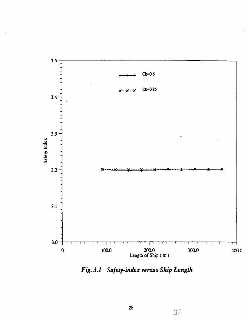
which we perform reliability analysis (CALREL) to determine the safety index for every
ship. The result is listed in Table 3.1 and is also plotted in Fig. 3.1. The ~’s in Fig. 3.1
are very close to each other (3.1980 < ~ < 3.2022), as compared to the range of ~ derived
from ABS Rules. Therefore, the calibrated model for the section modulus that gives
uniform safety for all ship sizes is given by Eq. 3.1 with
Ysw= l,l(j3yw = 1.15
* = 0.86.
26

L(m) Ch p(L/B=5.o)
91.5 0.60 3.1999
0.85 3J?012
122.0 0.60 3.1988
0.85 3.2004
152.5 0.60 3.1980
0.85 3.1998
183.0 0.60 3.1982
0.85 3.2000
213.5 0.60 3.1989
0.85 3.2001
244.0 0.60 3.2005
0.85 3.2015
274.5 0.60 3,1992
0.85 32017
305.5 0.60 32010
0.85 32018
355.5 0.60 3.2015
0.85 3.2020
366.0 0.60 3.2018
0.85 3.2022
Table 3.1 Safety Indices of Redesigned ABS Ships
2737
3.4
3.0 1 1 1 I 1 1 I II
I 1 1 1 T 1 I 1 TI
1 1 T 1 T T I 7 1I
I 1 1 1 I 1 I
o lUI.O 200.0 300.0 400.0Length of Ship(m)
Fig. 3.1 Safety-index versus Ship Length
28

3.3 Benefits of the Calibration
The main benefit that accrues from the redesign exercise according to the new safety
check format is uniform reliability and structural safety among different ship sizes,
whichin some cases could lm.d to weight savings. Code calibration exercises such as this
can highlight sometimes large differences in implicit safety levels for different failure
modes in a structure, a situation that can be rectbled in a new generation reliability based
code.
29

30
4/

4. Development of Limit States for an Example Ship
As stated earlier, the objective of this part of the study is to demonstrate how to use
reliability technology to assess the level of risk associated with an existing ship or with a
“drawing board” design. For this purpose an existing tanker was selected as an example
in consultation with the Project Technical Committee.
Several limit states are formulated and applied to the example ship. These are: the
ultimate limit states (deck yielding, fully plastic collapse, and instability collapse), the
semiceability limit state (local buckling), and the fatigue limit state for one point in the
deck. Because the maximum stillwater bending moment of the example ship occurs in
sagging condition, only this condition is considered for the ultimate and semiceability
limit states. Details of all calculations are given in Appendices 3 through 7.
4.1 Selection of the Example Ship
A tanker designed
characteristics are:
Displacement
L.O.A
L.B.P
Beam
Depth
Draft
CB
accofllng to ABS Rules is selected as the example ship. The main
*149,000 tonnes
273.0 m. ( 895.1 ft )
260.0 m ( 852.5 ft )
42.0 m ( 137.7 ft )
23.5 m ( 77.0 ft )
16.0 m ( 52.5 ft )
0.710
The elastic section modulus at deck is 4.657675”105 m-cm2 (236,851 inz-ft). The
nominal yield strength of the material used is 259 MPa (37.4 ksi).
4.2 Formulation of Limit States
1.
As mentioned earlier the limit states considered in this demonstration are:
Ultimate strength limit state
31L/,3

2. Semiceability limit state
3. Fatigue limit state
For ships, ultimate limit states can be decomposed into two modes of failure:
a. Failure due to spread of plastic deformation, as can be predicted by plastic limit
analysis and fully plastic moment ( initial yield and shake down moments can be also
classified under this category ) [6].
b. Failure due to instability or buckling of longitudinal stiffeners ( flexural or tripping )
or overall buckling of transverse and longitudinal stiffeners of grillage.
Serviceability limit states are associated with constraints on the ship in terms of
functional requirements such as maximum deflection of a member or critical buckling
loads that cause elastic buckling of a plate.
Fatigue limit states are associated with the damaging effect of repeated loading which
may lead to loss of a specific function or to ultimate collapse. This particular limit state
requires an independent type of analysis.
4.2.1 Ultimate Mrerwth Limit States
Three failure modes due to the combined action of wave and stillwater bending
moment are considered. The ultimate limit state can be described as:
C@w-tfw<o (4.1)
where
au is the ultimate hull girder moment capacity as determined by the critical stress of the
respective failure mode and the effective section modulus.
~ is the still-water bending moment.~ SwMw is the wave bending moment.
Mu is determined for each failure mode as follows:
Deck Initial Yield
Because buckling of the plates in the deck occurs before the deck initial yield, the
effective section modulus after buckling is applied. The ratio of the effective section
32

modulus to the elastic section modulus is calculated to be 0.98 (see 3.3 of Appendix 3).
The critical stress is then the material yield strength:
SMeff = 4.57*105 m-cm2
~cr = 259 MPa
‘Y
J?ullv Plastic Co law1
The plastic section modulus for the example ship is calculated according to [7], and
the critical stress is the material yield strength. The details of the calculations are given
in 3.1 of Appendix 3.
SMP = 5.8376*105 m-cm2
acr = 259 MPa
= ay
Bucklinv INa bilitv
The elastic section modulus is used and the critical stress is the buckling stress found
by applying the approximate equations described in [8]. These equations are based on
beam and plate theories for elastic and plastic buckling. The elastic section modulus of
the tanker at deck is:
SMe = 4,657670105 m-cm2
and the critical stress due to buckling depends on the buckling mode as follows:
a. Plates between stiffeners
The plates between the longitudinal stiffeners are considered as simply supported
isotropic plates under uniaxial compressive load. The plate collapse str&s is (see 3.2 of
Appendix 3):
‘cr = 238 MPa ( ~ =0.92 )
33

b, Stiffeners and effective plating
For column buckling of longitudinal stiffeners only the ultimate limit state is
considered because when a column buckles it reaches its ultimate strength immediately.
The effective plating is determined from buckling considerations since the plate is under
edge compression. The calculations shown in 3.2 of Appendix 3 give a critical stress for
pm flexural buckling as:
% = 248 MPa (g = 0.958)
However, coupled torsions.1./flexuralbuckling stress must be also checked. For the
example tanker, deck longitudinal stiffeners have a single plane of symmetry which
means that the ultimate limit state is probably governed by a combination of torsional
and flexural buckling. For this condition, the critical stress is (see 3.2 of Appendix 3):
Ccr = 170 MPa
c. Cross-stiffened panels
Buckling of an entire stiffened panel, including both longitudinal and nansverse
stiffeners is considered assuming uniaxial compressive load. A panel between transverse
and longitudinal bulkheads
buckling stress calculations
stress for the entire panel is
acr = 259 MPa
is shown in section 3.2 of Appendix 3 together with the
according to reference[8]. The resulting critical buckling
d. Summary, Buckling Limit State Strength
Plate between stiffeners 238 MPa
Flexural buckling of stiffeners 248 MPa
Tripping of stiffeners 170 MPa
Cross stiffened panels 259 MPa
34

These are local modes of failure. The ultimate hull girder collapse moment is
calculated in item e. below.
e. Hull Girder Instability Collapse
In the 1991 ISSC proceedings, report of the Committee on Applied Design[9], the
following expression was used for the approximate determination of a hull girder
instability collapse moment in sagging condition:
Mu= (.0.172+ 1.548$Cp-0.368$cp2)~SMe~Y
$CPis the compressive strength factor given by:
%p = (0.960+0.765k2+0.176B2+0.131k2B2+I.046k4)-O”S
where
k is the column slenderness of a critical panel,and
B is the plate slenderness ratio.
Appendix 4 shows the calculations of the factor $Cp for the example tanker and the
resulting ultimate moment “MU”.
$cp= 0.79 and
Mu= 0.82 SMe”~Y
4.2.2 Serviceability Limit States
The serviceability limit state
limit state:
% seN. - Gsw -Gw<o
where
N
These values are
can be expressed in the same form as for the ultimate
(4.2)
MseN. is the hull moment capacity as determined by the critical buckling stress ina serviceability limit state.
35

Gswis the stillwater bending moment.
GW is the wave bending moment.
The critical buckling stress of local plates between stiffeners is calculated for the
example ship in 3.2 of Appendix 3. The elastic section modulus is applied. These values
are:
SMe = 4.65767D105rncm2
=Cr = 227 MPa (a = 0.870 )‘Y
4.2.3 me Limit State
The fatigue limit state is associated with the damaging effect of repeated loading.
There are two approaches to the fatigue problem, the Palmgren-Miner approach based on
S-N cu.wes, that will be used here, and the fracture mechanics approach.
The S-N cues are obtained by experiments and give the number of stress cycles to
failure. Such curves are of the form:
NoASm=C
where
N is the number of cycles to failure
AS is the stress range
m is the inverse slope of the S-N cume
C is determined from the S-N curve by
IOgC = @ a ‘z~I.gN
where
a is a constant referring to the mean S-N cume~logN is the standard deviation of logN
The fatigue life calculation is determined based
cumulative damage (Palmgren-Miner rule). Application
36
(4.3)
(4.4)
on the assumption of linear
of this assumption implies that

the long-term distribution of stress range is replaced by a slress histogram consisting of
an equhmlent set of constant amplitude stress range blocks.
The time to failure of a detail can be expressed as [10] :
(4.5)
where
‘F is the value of the Palmgren-Miner damage index at failure.
~ and m are obtained from the S-N cumes.B is the ratio between actual and estimamd stress range.
!2 is a stress parameter.
T, AF, C and B are random variables. If the long-term distribution of the wave process is
assumed to be a series of short-term sea states that are stationary, zero-mean, Gaussian
and narrow banded, and if, in addition, the structure is linear, the stress range will follow
a Rayleigh distribution and Q is determined from[lO,l 1]:
*=@&(m-1)/2 1/2
~z r(l+~-XPjkOj kjj
(4.6)
where
Pj is the probability of occurrence of the j-th sea state.
hoj , ~j are the zero and second stress spectrum moments in the j-th sea state,
respectively. Note that &4
h is the freqbj
uency of the stress process in the
j-th seastate.
The fatigue limit state function is expressed as :
(4.7)
where ~ is the service life of the ship.
37

5. Development of Load Models for the Example Ship
From the information given on the Tanker example, the maximum stillwater bending
moment is 1.9728*106 kNm and it occurs in sagging condition. The maximum
allowable by ABS for this ship is 3.022-106 kNm.
5.1 Wave Bending Moment for Ultimate Limit State
The r.m.s. value of the wave induced bending moment on a ship can be estimated
from the seakeeping tables in [12]. Using the interpolation procedure described in that
paper, the rrns of the bending moment can be determined when the Froude number, the
sign~lcant wave height ,“Hs”, the beam/draft ratio, the length/beam ratio, and the block
coefficient are given. Knowing B/T, L/B, and CB for the example ship and assuming the
ship’s speed to be
12 knots for Hs ~ 3m
8 knots for 3m c Hs < 6m
5 knots for 6m c Hs.
The rms of the wave bending moment can be,approximately determined for any sea state.
The Wave Bending MornGIIJfor the Ultimate Limit State
For the ultimate limit state, an extreme sea condition is of interest. The most probable
extreme sea condition the ship is likely to encounter during its life time is determined
from the wave data along its route. The ship is assumed to remain in this peak sea
condition for three hours (which corresponds to N=1OOOwave peaks). A detailed
procedure for this short-term analysis is described in reference[6]. The wave loads in
this extreme sea condition are then determined and the corresponding safety indices for
the ultimate failure modes are evaluated.
Following this procedure for the example tanker, the rms of the wave bending
moment is determined for a significant wave height of 12.2 m (40 ft.). Section 5.1 of
Appendix 5 shows
bending moment is
6 =rms=
the calculation procedure. The resulting nns value of the wave
1.25398.106 kNm (5.1)
3851”
Assuming that the wave bending moment follows the same distribution as described in
Section 2.4.2 with N=1OOOpeaks, the mean value is determined by Eq. 2.3 to be
4.855=106kNm. For comparison, the wave bending moment given by 1991 ABS for the
example ship is 4.62*106 kNm.
Note that the above calculations are for a seastate of 12.2 m (40 ft) wave height. This
particular seastate is used for illustrative pruposes. For design, a storm condition with
specified return period should be selected including several pairs of representative
significant wave heights and characteristic periods. The most critical ship response can
be thus determined.
5.2 Stress Ranges and Number of Cycles for Fatigue Limit State
The sea scatter diagram given in the ISSC proceedings[9] and shown in section 6.2 of
Appendix 6 is applied. The rms value for every sea state is determined and the
calculations and the results are included in section 5.2 of Appendix 5. The scatter
diagram used is for the Osebery area of the North Sea.
39
37
6. Reliability and Safety Indices of the Example Ship
In this section, the reliability of the example tanker considering both the ultimate and
fatigue limit states is determined. Model uncertainty will be included in all limit state
formulations in order to reflect errors resulting from assumptions and deficiencies in
analytical or empirical design models and equations.
6.1 Ultimate Limit States
The sagging condition is considered and the limit state is expressed as:
where
S-M is section modulus.~m is the critical failure stress.
fisw is the stillwater bending moment.
~w is the wave induced bending moment.
;U is model uncertainty on strength.
:Sw is uncertainty in the model of predicting the stillwater bending moment.
~w is the error in the wave bending moment due to linear seakeeping analysis.
IS takes into account nonlinearities in sagging.
The tilde denotes random variables.
The distribution of model uncertainty parameters are shown in Table 6.1
random variable distribution mean C.o.viu N (NOllllZd) 1.0 0.15
z-Sw N 1.0 ‘ 0.05
:W N 0.9 0.15XR N 1.15 0.03
(6.1)
Table 6.1 Distributions of Model Uncertainty Parameters
40

6.1.1 Reck ~
Two cases of the stillwater bending moment are considered
In CASE 1, the stillwater bending moment is treated as a deterministic quantity equal
to 3.022”106kN-m, which is the ABS maximum allowable stillwater bending moment
for this ship. The effective section modulus is taken as the mew value. Table 6.2 shows
the means and coefficients of variation from Ref. [6] of the random variables not shown
in Table 6.1.
random variable distribution mean C.o.v
SWM LOgnormal 4.57*105m cm2 0.04~rr Lognormal 25.9 kN/cm2 0.07
%W Extreme 4.855*106kNm 0.09
Table 6.2 Distributions of Random Variables ,CASE 1
Appendix 7 shows the input/output files from CALREL printout. The safety index (~)
equals 1.81, which implies that if the ship,while loaded at its maximum allowable value
of the stillwater bending moment, experiences a three hour storm with significant wave
height of 12.2m (40 ft) the probability of failure due to deck yielding is Pf = 3.5*10-2for
this severe storm.
In CASE 2, the stillwater bending moment is treated as a random variable with mean
equal to 0.6*3.022*106to be consistent with Eq. 2.2. Tables 6.1 and 6.3 give the random
variables and their distributions. From CALREL for this case, the safety index (~) equals
2.25, which implies a probability of deck yielding of Pf = 1.2*10”2.
The effect of correlation between the stillwater bending moment and the wave
bending moment is investigated next. This correlation arises because of a weak
dependence of the wave bending moment on the loading condition. CASE 2 is repeated
with a comelation coefficient of 0.2,0.5, and 0.8. The results are ~= 2.23, ~=2. 18, and&
2.13, respectively for this severe storm. This indicates that the reliability index is not
very sensitive to this correlation and it is therefore neglected in the following analyses.
415.3
random variable distribution mean C.o.v
SmM Log-normal 4.570105 m cm2 0.04Em LOgnormal 25.9 kN/cm2 0.07
G.w Normal 1.8130106 kNm 0.40
%., Extreme 4.855*106 kNm 0.09
Table 6.3. Distributions of Random Variables ,CASE 2
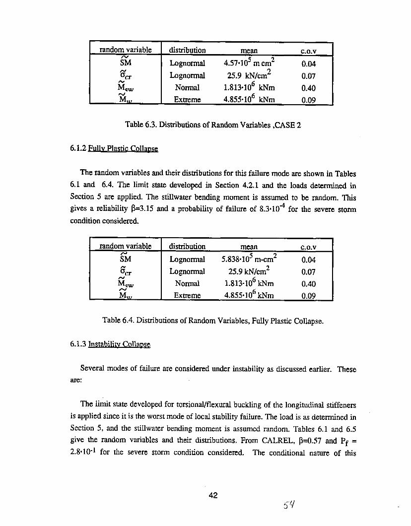
6.1.2 Fullv Plastic Collam~
The random variables and their distributions for this failure mode are shown in Tables
6.1 and 6.4. The limit state developed in Section 4.2.1 and the loads determined in
Section 5 are applied. The stillwater bending moment is assumed to be random. This
gives a reliability ~=3. 15 and a probability of failure of 8.3*104 for the severe storm
conthtion considered.
random variable distribution mean C.o.v
~M Lognormal 5.838*105m-cm2 0.04
Ecr Lognormal 25.9 kN/cm2 0.07
G.w Normal 1.813.106 ENm 0.40
Zw Extreme 4.855*106 kNm 0.09
Table 6.4. Distributions of Random Variables, Fully Plastic Collapse.
6.1.3 Instability CollaDs~
Several modes of failure are considered under instability as discussed earlier. These
are:
The limit state developed for torsional/flexural buckling of the longitudinal stiffeners
is applied since it is the worst mode of local stability failure. The load is as determined in
Section 5, and the stillwater bending moment is assumed random. Tables 6.1 and 6.5
give the random variables and their distributions. From CALREL, ~=0.57 and Pf =
2.8*10-1 for the severe storm Confition conside~d. The ~ondition~ name of this
42

probability is emphasized. It is conditioned on encountering this severe storm condition,
which is small. The mode of failure is also local.
The hull girder instability collapse according to section 4.2. l.d is considered nex~
This gives a mean value of acr = 212 MPa. All other variables remain as given in Table
6.5. The resulting safety index is ~ = 1.49 and Pf = 6.8-10-2, again conditional on the
severe storm condition considered.
random variable distribution mean C.o.v
S$M LOgnormal 4.6580105 m-cm2 0.04Fcr Lognomml 17.0 kN/cm2 0.07fiqw Normal 1.813*106kNm 0.40
%., Extreme 4.855*106 kNm 0.09
Table 6.5. Distributions of Random Variables, Instability Collapse
6.2 Fatigue Limit State
Figore 6.1 shows the analyzed detail, which is a welded deck longitudinal to the deck.
It is classified as class D according to classification given in reference[13]. The analysis
is concerned with one fatigue location. No system aspects are considered. The limit
state function is given as:
(6.2)
d
Xw is included in the limit state as a modeling uncertainty to take into account the error
in wave bending moment prediction using linear analysis. The other variables are as
described in Section 4.2.3. The stress parameter, calculated in section 6.1 of Appendix 6,
is !2 = 852 [ MN/m2]3[sec]-l and from the S-N cue, the mean value of C = 1.52c1012
MN/m2.
The analysis is performed with the random variables distributed as shown in Table
6.6. The reliability index ~ equals 2.44, and the probability of failure is 7.3”10-3 over a
lifetime of 20 years.
43.<”%5-

Ion.giludinalstiffener(450 x 30)
deckpklletz~] mm
-+Ft&+f-1 A
5400mm D Dmsvcrscfrdmc !480x 35
dwk@C
A-A
Figure 6,1 Detail Considerd in the Fatigue Analysis.
random variable distribution C.o.v
~F bgnormal 1.44 0.15
E Lagnormal 1.52”10’2 0.40
5 bgnomud 1.02 0.10.wXw Normal 0.%) O*15
Table 6.6, Dkrnbutions of Random Vtiables, Fatigue
44

6.3 Summary of Safety Indices
The following is a summary of the calculated probabilities of failure:
a) Deck initial yield 0.012 (Global)
b) Fully plastic condition 0.00083 (Global)
c) Instability (tripping) 0.28 (Local)
d) Hull girder ultimate moment 0.068 (Global)
,.
e) Fatigue, 20 years 0.007 (Local)
It is to reemphasized that these values are conditional on the severe scastate assumed,
in the case of items a) through d). The unconditional probabilities of failure are expected
to be lower since the shown Values in items “c” and “d” must be multiplied by the
probability of encountering the severe storm condition used in their calculations. The
fatigue (item e) is unconditional Value calculated for one detail over the 20 year life of
the ship.
45
.5-7

T 3 Stru~v P OCfISS Defnltlw. ., .,
r I
46

7. Terminology Associated with Structural Reliability
The aim of this chapter is to define the terminology associated with the structural
reliabfi~ of ships and offshore structures. The fo~owing are considered
“ Load terminology
- Strength terminology
. Structural reliability terminology
The terminology defined addresses those terms associated wit-bprobability, statistics and
reliability as used in engineering.
7.1 Load Terminology
The following tenus are primarily used with loads, although some of the terminology
is more general, and related to statistics and random processes.
Deterministic Proce~
If sn experiment is perfonmd many times under identical conditions and the records
obtained are always alike, the process is said to be deterministic. For example, sinusoidal
or predominantly sinusoidal time history of a measured quantity are records of a
deterministic process.
Random Process
E the experiment is performed many times when all GanditiQn$under the. Can&d d
the experimenter are kept the same, but the records (usually a time history) continually
differ from one amther, the. process. is-said to be random. TIE. degree. of randomness.
depends on (1) understanding of the factors involved in the experiment results, (2) the
&i& tOWlltPOitkll!l. The OUtC~ Ofa F- PHKeSSat ~~ giWll irlStZ@d ~ iS
a random variable. Time history of wave elevation and strain gage records taken aboard
a ship maybe mmidered as random processes.
Random Variable
Different vahes of a random vm”abIe have different chances (frequencies) of
mxurr~ A random vtible th~ has a pbabili~ density function. Examp.k of
47

random variables are the wave bending moment, the still water bending moment, and
material yield strength.
Probability Densitv Function
The probability density function defines the relative frequencies of occurrence of a
random variable (e.g., wave height or wave bending moment). The function, usually
denoted f(x), where X is the random variable, has the following properties:
x
1)
2)
3)
4)
The probability of occurrence of fraction of the random variable
between x and x+dx is f(x)dx, i.e.,
P[x < X < X+ dx] = f(x)dx
The probability that a sample of the variable lies between a and b is:
The probability that X lies between -= and +Mis unity.
P[x = a] = Owhere a is a constant.
x which lies
Distribution Function
Also called the cumulative distribution function, and denoted F(x), this defines the
probability that the random variable X is less than or equal to a given value x, i.e.,

F(x) = -~~f(x)dx
F(x)
1.0 ——————————
x
Fxceede ce Robabd w..’
n 1
This is the probability that a random variable X (e.g., wave bending moment)
exceeds a specifkd value x, and is given in temns of the probability dismilmtion function
as 1- F(x), since
$()x
x

Percentilg
keentikwdsdi+r*~X amtbsevaitmt Cm=pdbg. to Speeifssvalues of the cumulative disrnbution function F(x). A 50-percentile value thus
corresponds to x such that F(x) = 0.5. This particular percentile is also the median value
of the random variable. A 95-percentile value is a value such that F(x) = 0.95, i.e., only
5% of the outcomes of the random variable are expected to lie above it.
x
Mean. Median and Mode
For a given probability density function f(x) relating to a random variable X, the
mean or average value p is given by
~= E(x)= f~X f(x)dx
where E(x) denotes the “expected value” of X,
The median value of X, denoted ii, is defined from the cumulative distribution
function F(x) as
%= F-l (0.5)
50 [,’/
i.e., it is a value of X corresponding to a cumulative distribution function of 0.5. This
implies that, on the average, 1/2 the outcomes of the random variable will lie below i
and 1/2 above it.
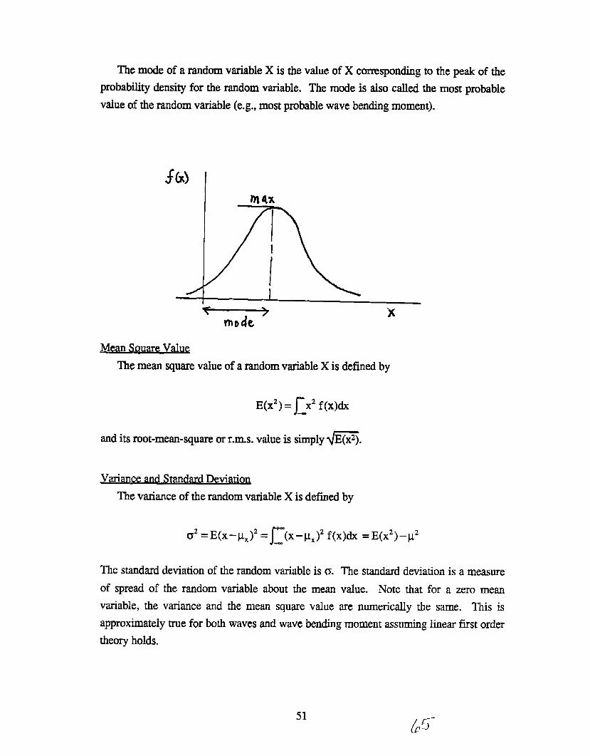
The mode of a random variable X is the value of X corresponding to the peak of the
probability density for the random variable. The mode is also called the most probable
wdue of the random variable (e.g., most probable wave bending moment).
m 4X
Mea Square Va uen 1
The mean square value of a random variable X is defined by
E(x2) = ~X2 f(x)dx
and its root-mean-square or r.m.s. value is simply ~~.
uce and Standard Devi-
The variance of tie random variable X is defined by
a2=E(X+LX)2 = j’jX -~x)2f(x)dx = E(X2)–L2
The standard deviation of the random variable is a. The standard deviation is a measure
of spread of the random variable about the mean value. Note that for a zero mean
variable, the vtiance and the mean square value are numerically the same. This is
approximately true for both waves and wave bending moment assuming linear frost order
theory holds.
51(j5-t

Coefi. .
cient of Vanan on
The coefficient of variation 8 of a random variable X is defined by
6=:n
where ~ and p are the standard deviation and the mean value. The coefficient of
variation is a non-dimensional measure of the spread of the random variable outcomes
about the mean value. The coefficient of variation of wave heights and wave bending
moments over along period of time is expected to be high (80-100%). The coefficient of
variation of the extreme values of these quantities over a short period of time in a severe
sea state is much smaller (7-20%).
Joint Pmbab.
ilitv Densitv Function
The joint probability density function of two random variables xl and Xzdefies the
frequency of mutual occurrence of two random variables and has the following
properties:
1)
2)
3)
A
where n indicates the mutual occurrence (intersection) of two events.
related joint distribution function deftig cumulative probabilities may also be
defined. The deftitions maybe extended to more than two random variables.
The joint density and distribution functions for random variables contain the
occurrence probability and also conflation infomuation.
52

covan~.
The covariance of two random vtiables, Xl and Xz is defined as
= j-~ (x,-Px,)(x2-vx2 )f(x,*x2)~,~2--
where pX,and p.xzare the means of the individual random variables, and f(xl, X2)is their
joint density function.
Indeue@ent Random Variabl~
Two random variables Xl and Xz are independent if their joint density function is
equal to the product of their individual densities
f(x~, X2) = f(x~) f(?@
where f(xl, @ is the joint density function and f(xt] and f(@ are the individual @so
called marginal) density functions. The outcomes of independent random variables occur
without any reference to one another. Normally in reliability analysis, strength and load
are considered independent random variables.
Det)endent Random Variables
Two random variables Xl and X2 are dependent if their joint density function is not
the product of the marginal densities. The outcome of any one of the random variables is
dependent on tie outcome of the other, i.e., there is a correlation between the realization
of one random variable and realizations of the other. For Xl dependent on X2, the
following is true:
fx,x, (xl/ X2)f(xl [X2)=
ftxJ
where f(xl/xz) is the conditional density, f(x2) is a marginal density, and ~x,x~(xl/ Xz) is
the joint density evaluated with xl given X2
53 &---

Bounded Random Vambks.
The deftitions of probability density and distribution functions given in this section
assume that random variable outcomes lie in the interval -= < X e -. Here, the bounds
on the random variable are -= and w. For some rsndom variables, the upper and/or
lower bounds may be different. For example, material yield strength is always a positive
quantity, and its lower bound is zero. An upper bound on a load is sometimes used
resulting in a truncated probability density function.
CoIIelation Coefficien~
The correlation coefficient pq+ for two random vaxiables Xl and Xz is defied by
where V%~ is the covariance of xl and X2,and the o are the standard deviations. The
correlation coefficient always lies between -1 snd +1. If the correlation coefficient is
zerw, the variable outcomes me uucmrdated. The corrdatim coeflk%mt is a frrst order
measure of dependence between outcomes of two random variables. A zero correlation
is a weaker condition than independence. Non-con-elated random variables are not
necessarily independen~ but independent random variables are necessarily uncomelated.
Positive correlation means that, in general, if the outcomes of one random variable
increase, the outcomes of the other will also increase. Negative correlation means that
the outcomes will generally be in opposite directions.
The wave bending moment is weakly correlated to the stillwater bending moment
since both depend on the weight distribution along ship length.
. . . .lhOnd Probabdltv and 13avesTheorem
A conditional probability is denoted P[A/B] when A is one event and B is another
event on whose outcome A depends on. An example of a conditional probability is a
probability of structural failure calculated for a given sea state. The actual lifetime
probability of failure will be different if all the sea states are considered. Bayes’
Theorem applies to conditional events. By Bayes’ Theorem, the probabtity that event A
occurs conditioned on the probability that event B has already occurred is given by
P(A /B)=P(AnB)
P(B)
54

where A and B are the event domains and AnB is their intersection, i.e., the outcome
space that contains both A and B at the same time (mutual occurrence).
~om Proc~
A random process is stationary if the probability density function of its outcomes
does not depend on time, i.e., the same probability density fimction is obtained for an
ensemble of mlizations of the random process at any given time as at any other time.
This also means that statistics that are dependent on the probability density function, e.g.,
mean and mean-square value, are also independent of time. The second order (joint)
probability density function of the outcomes at two instants of time depends on the time
lag between them and not on each individually. Tme history of waves or wave bending
moment are usually considered stationary over a short period of time [up to 3 hours).
@odIc Hypot.
hem
This states that a single sample function is quite typical of all other sample functions
representing realization of a random process. Therefore we can estimate the various
stmistics of interest by averaging over time using the one realization raiher than
averaging over an ensemble of realizations. An ergodic random process is necessarily
stationary. A stationary random process is not necessarily ergodic.
Exteme Value
The extreme value of a random process is the largest value over a period of time.
Each realization of the random process will have an extreme value. Thus there is also a
distribution of extreme values, i.e., the extreme value is a random variable that has its
own special distribution, mean value, variance, etc. One may spe~ therefore, of
extreme value distribution of wave heights or wave bending moments.
Most Probabl e Extreme Value
This is the value of the random variable corresponding to the peak of the extreme
value density function, i.e., the mode. Thus, the most probable extreme wave bending
moment is the mode value of the extreme bending moment density function, i.e., the value
of the moment at the peak of the density function.
Asynmtotic Distributions of the Extreme VaIu~
The extreme value distribution for a random process with defined probabili~
characteristics for the outcome (e.g., a Gaussian random process) is a function of time, or
equivalently, the number of peaks within the time. As time or number of peaks increase,
55
the disrnbution of the extreme value shifts to the right. The asymptotic distribution
corresponds to an infinite length of time or number of peaks. The asymptotic fomn of the
extreme value distribution depends largely on the tail behavior of the “initial” distribution
of outcomes of the random process. Gumbel showed that the asymptotic distribution
takes one of three forms: a double exponential form, an exponential form and an
exponential form with an upper bound.
Order S~. .
The disrnbution of the largest peak (e.g., largest wave bending moment) in a
sequence of N peaks of a random process can be determined using order statistics,
assurohg that the peaks are independent and identically distributed. The cumulative
distribution function of the largest peak is given by
Fz~(Z) = P[max (ZI,%,...,Q *I
= ITZ(X)IN
where FZ(z,e) is the i.qitial cumulative distribution function of the peaks and E is the
spectral bandwidth parameter. The corresponding probability density function is given
by differentiating the cumulative distribution function:
fzN(z) = N~Z(Z,E)]N-l. fZ(z,&)
where fZ(z,&)is the initial p.d.f. of the peaks.
Exnected Maximum Value:
The expected value (average) of the maximum peak (e.g., wave bending moment) in
a sequence of N peaks of a zero mean Gaussian random process was determined by
Cartwright and Longuet-Higgins, and is approximated by
where C = 0.5772 = Euler’s constant. Here, mOis the area under the power spectral
density, i.e., the mean square value of the process.
It should be noted that the most probable extreme value (i.e., the mode) is given by
the above equation, but with the second term on the right hand side deleted.
56
~~
This is a random process whose time realizations are such that there is one peak
between every uperossing and every downerossing of the mean level. Process “cycles”
are thus discernible. The power spectral density function of the process realization has a
central tendency, i.e., it is clustered about a central frequency. The peaks of a zero mean
narrow band Gaussian random process have the Rayleigh distribution function given by
where mOis the mean square value of the process, also equal to the area under the energy
spectrum for the process.
Records of waves and wave bending moments over a short period of time (3 hours)
are usually considered to be narrow-band processes.
Avers ~~
This is the average value of the highest l/m-th peaks in a random process. For a
random process whose peaks are Rayleigh distributed,
Average of 1/3 highest vaIues =26
Average of 1/10 highest values= 2.55&
Average of 1/1000 highest values =3.856
where mO is the mean square value of the process. The multipliers shown are for
amplitudes rather than heights (double amplitudes). The average of 1/3 highest values is
also called the significant value. These multipliers may be used for waves and wave
bending moments and may err slightly on the Ccmservativeside.
7.2 Strength
57“7/
The following terms related to strength are now defined: failure modes, limit state
function, and ultimate, serviceability and fatigue limit states. Limit state exceedence
probability is then defined, and contrasted to the probabWy of failure. Also in this
section, terminology related to the classification of uncertainties is given. Some of this
terminology is geneml, but their use is relevant to strength variability, and illustrated
with strength parameters. System failure modeling is also considered in this section.
Failure Mod&
A failure mode refers to a particular physical mechanism by which a structure or a
part of it fails. Failure mocks for ships address plastication, buckling, fatigue and
fracture. ASan example, buckling failure modes include plate buckling, stiffener flexural
buckling, stiffener tipping, and overall buckling of the gross panel.
Ulhmate Lumt State.. . . .
The ultimate limit state considers structural performance or safety margin under
extreme (typically lifetime maximum) loads. The ultimate limit state can be further
decomposed into two modes of failure:
& Failure due to spread of plastic deformation, e.g., as predicted for beams by plastic
limit analysis. The initial yield moment for a beam can also be classified under
this category.
b. Failure due to instability or buckling, e.g., of panel longitudinal stiffeners in the
flexura.1 and tripping modes, or the overall “gtillage” buckling of a gross panel
consisting of longitudinal and transverse stiffeners.
. .eabtkw Limit Stt@
The serviceability limit states are associated with constraints on the marine structure
in @Tns of functbnal requirements such as the nmirnurn d~ection of a member or
critical buckling loads that cause elastic buclding of plating.
Fatkue Limit Stat%:
The fatigue limit state is associated with the damaging effect of repeated loading
which may lead to a loss of specific function or to ultimate collapse. Fatigue limit state
capacity for structural details is typically defined using S-N curves, while the demand is
defined interns of the lifetime stress range versus number of cycles histogram.
~imit State Funcnoq:
This is a function, often denoted G@ where ~ is a vector of basic variables, that
characterizes the safety margin in a given mode of failure. A simple limit state function
may be
58

G(cy, a) =Uy-a
where aYis the yield strength of the material, and o is the load effeet (stress). Note that
limit state exceedence (“failure”) implies
Limit state functions are traditionally formulated in this capacity minus demand form.
The basic variables in the limit state equation are random because of inherent variability
or model uncertainties.
Limit State Exceedence Probabilim
The probability of reaehing or exceeding a specd%d limit state is determined from
where f=(xJ is the joint probability density function of the basic variable vector X. The
domain of integration F is over the unsafe region of the limit state function where
demand exceeds capabtity. The integral is multi-fold. In temns of the limit state
equation, the domain of integration is defined by G(K) S O. To the extent a limit state
equation may address local phenomena, e.g., yield at a point, serviceability, e.g.,
deflections, etc. in addition to catastrophic events, interpreting the limit state exceedence
probability as the pmbabikty af “failure” of the structure should be done with care.
It Amul.dalso be noted that limit state exceed.ence pmbabiktks calculated =e often
conditional on certain environmental events, e.g., occurrence of a certain severe storm.
babilitv of Failure
Although actuarially speaking, this should refer to the probability that the structure
catastrophically fails, the texm is generally and widely used as a substitute for limit state
exceedence probability, i.e., the probability that the demand exceeds the capability in any
given limit state (including exceedence of deflection and elastic buckling stress).
Uncertaintv Classification
Uncertainties which conrnbute to the variability of physical strength parameters may
be classifwi as
59
● inherent uncertainties
. model unce~ries
They may also be classified as subjective and objective uncertainties. The ckssiiications
while illustrated here with strength parameters, are also relevant to loads and load
llmdels.
Oblectwe lJnc~. . . .
These are uncertainties associated with random variables for which statistical data can
be collected and examinal They can be quantified by a mean, a coefficient of variation,
and a form of the probability distribution function derived from available statistical
information. l%e variability in the yield strength of steel is an example.
$ublecnve U cetia,.
n “ntie$
These are uncertainties associated with the lack of infmmdon and knowledge. They
are typically quantified on the basis of the engineer’s prior experience and judgement.
Examples of these include assumptions in the analysis, error in the design model, and
empirical formulae. The following subjective uncertainties contribute to strength
variability:
a) Effectiveness of plating, e.g., due to shear lag
b) Use of Navier hypothesis in calculating hull girder response
c) Initial deformation and residual stress effects
Inherent Uncertainties
This kind of uncertainty is inherent to the variable, and csnnot be reduced because of
additional information. This is a term that in many cases may involve the same sources
as “objective” uncertainties. Examples are the inherent variability of wave heights,
extreme wave bending moment or the variability in yield strength.
Model lJncertaintie~
These uncertainties arise because of errors in the prediction models as they represent
reality. They can be reduced with additional information. Model uncertainties are
typically estimated based on comparing the analysis procedure with experimental data, or
in some cases using professional judgement or other indirect information such as the non-
occurrence of cracks in reiation to expectation. Some sources of modeI uncertainties are
described under “subjective uncertainties”. The largest model uncertainty in marine
60

structures usually relates to loads such as slarmning loads. Slrength prediction
techniques (e.g., for buckling strength) also have their own model uncertainties. This
type of uncertainty is usually quantifmd in terms of a bias (i.e., actual value to predicted
value ratio) and a coefficient of variation.
Structural Svstem Modeling
The behavior of a structure that can fail in more than one mode of failure is modeled
for structural reliability evaluation purposes using structured representations of system
behavior. Series, parallel or general system representations are usual. A genertd system
~pmsentation may take the form of a cut set (parallel subsystems connected in series)
representation or a link set (series subsystems connected in parallel) representation.
Failure tree representations are also possible. Reference is made to [6].
Series Svstem:
A series system is one that is composed of links connected in series such that failure
of any one or more of these links constitute a failure of the system, i.e., “weakest link”
system. In the case of the primary behavior of a ship hull, for example, occurrence of
any one of a number of modes of failure will constitute failure of the hull. The multiple
failure modes can then be modeled as a series system.
Parallel Svstetq
In a parallel system, @l links along the failure path must fail for the structure to fail.
ArI example is a multicomponent redundant structure such as a freed offshore platform,
in which a fa.dure path is the failure of a group of members which leads to system
collapse. The faiLureevent resulting from one failure path can be modeled by a parallel
system.
Since there typically are many different failure paths, each represented by a parallel
system, and since failure can occur in any one of the failure paths, the entire system can
be modeled as a giant series system with parallel subsystems, each representing a failure
path.
7.3 Structural Reliability
In this section, we consider terminology related structural reliability, reliability
~ ati pmbabilistically based structural desi~ co.des-
61 -/5”

~
T& is the eompkmm d * probability of failure ~ i.e.,reliability k the
probability of survival, given by 1- p~
tvm “n
This is the difference between capacity and demand, or strength and load. Either
mean or characteristic values maybe used to determine the safety margin.
Level L )Sand HI Reliability Method$
The basic concept of Level III reliabtity methods is. that a probability of failure of a
structure always exists, and may be calcula~ by integrating the joint probability density
function of the variabIes invohd in the foad and strength aspects of the structure. The
&main & integmtion is the unsafe regim defined by the variables.
Because of the difficulties involved in determining the joint density function and in
calculating the multiple integration, Level H methods for obtaining the safety index and
the related probability of failure were introduced In Level II methods, the probability
content of the failure domain is obtained using approximations to the failure surface.
FORM and SORM, described elsewhere, are Level II methods. Primarily because of the
approximations made to the failure surface, and also because of approximations involved
in the inclusion of distribution information, the probabilities of failure calculated from
l..evelIImstlmdsmnGtmm. ~ ,themetlmd$ arevery effi&mt*-Esu#ya
good approximation is obtained
Level I refers to safety factor based design formats that are very similar to traditional
design formats and safety check equations, except that the safety factor(s) are obtained
on the basis of Level II methods to assure a certain target reliability level.
Safety Index:
The safety index is a number that is inversely related to the probability of failure.
The safety index ~ and the probability of failure are related by
Pf = W-B}
62
where @ is the standard normal distribution function. A safety index of 2.3 translates
roughly to a probability of failure of 1/100, 3.1 to 1/1000, and 3.7 to 1/10000. A safety
index of zero corresponds to a probability of failure of 0.5.
Hasofer-Lind Safew IndeT
In the history of structural reliability theory, there have been several definitions of the
safety index, some fell from favor because of a problem lmown as lack of invariance. By
this, it is meant that mechanically different limit state functions representing the same
physical f*e rnoderestthed in dWerent * of the safety *. The Hastiw-Liid
index does not suffer from the lack of invariance problem.
First Mcr Reliabilitv Method (FORNQ
The essential steps in this method of reliability analysis for the determination of the
probability of failure are:
a) The basic correlated random variables ~ defining the limit state function G@ =
O, with prescribed probability distributions, are transformed to a set of
independent standard normal variables ~.
b) The limit state surface g~ in the standard normal space is approximated by its
tangent hyperplane at the point of the limit surface closest to the origin. This
point has the highest probability density, and is called the design point or the
most probable failure point.
c) The probability content within the linearized failure domain is found as an
estimate of the actual failure probability. The FORM probability of failure is
where ~ is the reliability index, which is also the distance of the design point from
the origin in the u space. The FORM reliability index is invariant for
mechanically different limit state functions representing the same failure event.
Rackwitz-Fiessler Transformation
In calculating the safety index, it is necessary to include information related to the
form of the distribution of the basic variables. The tail of the distribution of the random
variables is usually the location where most of the contribution to the probability of
failure comes from. In the Rackwitz-Fiessler transformation, an equivalent normal
distribution is fitted to the tail of the nonnonnal distribution at the most Nely failure
point (design point). The method requires the cumulative distributions and the
63-) 7

probability density function of both the actual distribution and the normal distribution be
equal at the design point.
. . .er Re-tv Methods (SOR~
In SORM, the essential steps are similar to FORM, except that the limit state surface
in the standard normal “u” space is approximated by a second order approximation such
as a hyperparaboloid fitted with its apex at the design point. The failure domain
probability content within the second order approximation is then estimated. For
hyperparaboloids, the probability content can be “exactly” estimated.
In structural design, the performance of the structure is checked using safety check
equations. In the working stress approach for f~ed offshore platforms as embodied in
API RP-2A Recommended Practice, for example, the maximum or yield strength isdivided by a safety factor to obtain an allowable stress. Designs are then limited so that
the maximum calculated stress under extreme operating loads does not exceed the
allowable value. This example safety check is of the form
where R =
SF =
D=
L=
w=
R~>D+L+W+o~~lo~eff~ts
nominid component strength
safety factor
nominal gravity loads on components
nominal live load effects on components
nominaI environmental’~oadeffects on components
Nornimd loads are all combined with factors of one, and constant safety factors 1.67 and
1.25 are used for operating and extreme loadings. There are typically many safety check
equations to be satisfied in a design, each of which addresses a different failure mode or
design concern.
P“~~
A safety check equation in a partial safety factor format employs multiple safety
factors, which may address uncertainties in component loads, resistance, and also failure
consequences, non-coincidence of peak loads from different sources, etc. Because there
is more than one safety factor employed, the format is more efficient in that factors of
64 7’s’
safety are placed in a manner more commensurate with individual demands and
uncertainties. Also, the partial safety factors are usually obtained using Level II
reliability methods, consistent with a required target reliabtity level.
A sample psrdal safety factor format is that recommended in the Load and Resistance
Factor (LRl?D) version of API RP-2A. This is given by
@Ri~ > y~D+yLL+y~w+...
nominal strength or resistance of component i
partial resistance factor for component i
nominal gravity or dead load effect
load factor for dead load
nominal live load effect
load factor for live load
nominal environmental effect with prescribed return period
load factor for environmental load
Each resistance factor CDRiis calculated as a product of two factors, one representing
strength uncertain~, and the other taking into account the consequence of failure of the
component and the structural system. The load factors y are also calculated as a product
of two factors, one representing uncertainty in load intensity, and the other, uncertainty
in the related analysis procedures.
A partial safety factor foxmat is a Level I reliability based format if the safety factors
employed are obtained from reliability analysis with a prescribed target reliability.
Nominal or Charactel-lshc V-. .
Traditionally in structural design, nominal or characteristic values are used for the
basic design variables appearing iu safety check equations. For loads, characteristic
values on the high side of the mean are typically used, while for resistance, characteristic
values on the low side of the mean are used. Thus for example, in ship design, safety
check equations involving yield strength use the rule minimum yield, which typically is
about 15% lower than the mean value. The terms “characteristic” and “nominal” are
interchangeable, but sn occasional distinction appears in the literature where a
characteristic value refers to a nominal value that is selected on the basis of a probability.
For example, the characteristic yield strength may be a 5-percentile value, i.e. there is a
95% chance that the actual yield strength is greater than the characteristic value.
65
Code Caldmlam. .
This is the process of selecting a target reliability level and a corresponding set of
partial safety factors for use in a probability based design code. Reliability analyses of
comparable past experience (existing structures, and systematic structural designs to
traditional codes) are useful in the code calibration process.
. . .
This is the process of selecting partial safety factors for use in probabilistically based
safety check equations in such a manner that the scatter in the reliabili~ of structures
built to the code is minimized, and centered around the target value.
66

8. Extrapolation Techniques for Design Loads
In this chapter,extrapolationtechniques for determining lifetime extreme wave loads
ford.esign ase&ntifkL FOI p~O- of discussion I stn&stx “ wfwe hi p_mc~ iS
considered. The effective wave loads give rise to stress at a point, which include stresses
arising from hull girder bending in two planes, torsion, external pressure, internal tank
loads, etc. with proper accounting of phasing.
Extrapolation techniques for the wave load effect are fmt considered. The deftition
of design loads is subsequently investigated.
8.1 Identification of Techniques
There are two broad classes of techniques for the determination of the maximum
wave induced load over the vessel design life. These are:
a)
b)
Short term techniques, in which the short term statistical characteristics of the
wave load process in a stolm condition are used to obtain the distribution of the
extreme load and a characteristic design load.
Long term techniques, in which the long term distribution of the wave induced
load is obtained. That distribution includes within it all load peaks possible
considefig every seastate. A characteristic design load is then defined based on
the long term distribution.
The essential difference between the two classes of methods is that in the short term
approach, the extreme load distribution in a few high seastates is separately obtained for
each, and the characteristic design load is typically taken as the largest among values for
the various seastates, while in the long term approach, the design load corresponds to a
given exceedence probability (e.g., I&g) on the long term distribution. These two classes
of techniques are now described.
8.1.1 Short Term Wave Load Extrapolation
If the wave loads acting on a vessel can be represented as a stationary Gaussian
random process,, which is usually an adequate assumption over the duration of a seast.m
lasting a few hours, then at least two types of methods are available to predict the
67

distribution of the maximum load. These two methods, among others, are described in
detail by Mansour in [6]. In the fist method, the peaks are assumed to be statistically
independent and identicaDy distributed, and the distribution of the largest peak in N-
peaks is determined using classical order statistics. In the second, conventional
uncrossing analysis is used for determiningg the extreme value distribution.
A. Distribution of largest peak by order statistics
The distribution of the largest peak in a sequence of N-peaks can be determined using
Standard order Statistics. Consider a sequence of random variables, Zl, ~, ... ~
representing the peaks of a load on a marine structure. Assuming that these peaks are
identically distributed and statistically independent, the cumulative distribution function
of the largest one is given by
where FZ (z,E) is the initial copulative distribution function of the load peak (maxima)
and Gis the spectral bandwidth parameter defied from
Here, co is the radian frequency. The probability density function (pdf) of the largest
peak is determined by differentiating the c.d.f. with respect to z, thus
fw (z) = N~Z (z,&)]N-l. fZ(Z,&)
where fZ(z,E) is the initial p.d.f. of the load peaks. For an arbitrary bandwidth process,
the initial distribution of peaks within a short term seastate, considering positive maxima
alone, has been derived by Ochi (J. Ship Research, 1973). For a definition of positive
and negative maxima and positive and negative minima, see Figure 8.1. In the narrow
banded case, the conventional Rayleigh density and distribution functions apply.
68
Based on the Ochi distribution and order statistics, it can be shown that the modal
value, i.e., the most probable maximum load in N-peaks is approximated by
J= ‘“)]=FE--N})qnm(z1,z2,...
The qpuxinmtim wasderived by O&i comidering kge N and E <0.9. It can be
shown that there is a 63% chance that the largest response will exceed the modal value.
Other percentile values of the extreme value distribution were also obtained by Ochi, in
terms of a “risk parameter” m He chooses a very small number, u (e.g., 0.01) and
obtains a non-dimensional extreme value ~~ such that
[
~ Extreme value of maximain Npeaks > (N1=a
For E S 0.9, N large, and a small, it can be shown that
,.=f”The dimensional extreme value is equal to the non-dimensional
by ~.
extreme value multiplied
B. Extreme value distribution based on upcrossings
The distribution of the largest peak can be determined from uncrossing analysis of a
time history of a statiomuy random process instead of the peak analysis described above.
Principles behind the uncrossing analysis are described by Mansour (Ship Structure
Committee Report 351) and will not be repeated here. The essential problem is one of
determining the frost passage of a random process x(t) of a level “a” within a given time
interwd T. 13ase.don a level crossing analysis assuming that the individual level arrivals
are independent and Poisson distributed, it can be shown that the cumulative distribution
function of the largest x value, denoted Z, is
Fz (a) = exp (-vX(a) T)
69

where VX(a) is the expected number of level crossings per unit time. This is given by
Ha2
v= (a) = Vaew ,-~%
In the above, VOis the zero crossing rate, which for a namow band process, is
J1 mzVo=— —
27c mO
The above cumulative distribution function for the largest value ignores the tendency for
upcrossings to occur in clumps, because of the assumption of independence. The
solution ove~redicts extreme values. To consider clumping, an upper bound envelope to
the given process can be constructed, and the fiist passage probability for the envelope
process obtained. The uncrossing rate v~(a) for the envelope of a Gaussian process is
given in standard structural reliability textbooks as
) “
In general, this uncrossing rate will not lead to a
a— vx (a)r mO
decreased bound, since the envelope
may have excursions above the level without there being actual process upcrossings.
Such crossings are temzed “empty”, while otherwise they are called “qualilled’
upcrossings, a terminology devised by Vanrnarcke (ASME, J. Applied Mechanics, March
1975). Vanmarcke obtained an estimate of qualiikd excursions, which was later refined
using a Slepian regression model by Ditlevsen and Lindgren (J. Sound and Vibration,
1988).
To date, the Ditlevsen and Lindgren solution is the best available. Based on it, the
cumulative distribution function of the maximum value for an ergodic Gaussian narrow
band wave load p.miess. kcomes. @mer and Friis. Hamezq “Stochastic Modeling of the
Long Term Wave Induced Responses of Ship Structures,” submitted to Journal of Marine
structures):
70
r 1
where VE(a) was previously defied, “a” is the level value, and rv (a) is given, for
moderate spectral skewness, from
where
IImOmz72= ~; u= Q-
ml rmO
The extreme value analysis based on the uncrossing rate, as obtained above, provides
a cumulative distribution function of the extreme value, accounting for clumping of
peaks. It is derived for a murow band ergodic Gaussian wave load process, although
based on simulation comparisons, it seems applicable to relatively wide band processes
also. It is worth stating that the probability density function of the maximum value has
not been obtained.
C. Calculation of the short term extreme values
Short term extreme values based on the peak or level crossing analyses are calculated
seastate by seastate for several extreme wave conditions. Within a seastate, the extreme
values depend on (are conditional on) vessel heading and speed. Typically in treating
low frequency wave induced loads, the speed within a seastate is assumed constant and
extreme values conditional on different wave headings are obtained. The extreme value
for the seastate is obtained by unconditioning with respect to vessel headings, i.e., the
wave load extreme values for each heading are multiplied by the
71
heading probabilities
(&-

and added The largest characttistic extreme load among all seastates considered may
be used as a design load.
8.1.2 J.mIIrTerm . . .Wave Load llstnbu-
In the long term approach to the entire density
induced load is obtained, considering the following
or distribution function of the wave
(i)
(ii)
(iii)
(iv)
(v)
(vi)
(vii)
Frequency of occurrence of various sea states.
Frequency of occumence of various spectral shapes within each sea condition.
Ship route and frequency of encountering each seastate and spectral shape.
Frequency of occurrence of various vessel headings.
Frequency of occumence of various vessel speeds.
Frequency of occurrence of various ship loading conditions.
The expected number of load cycles for a given sea, wave spectral shape,
speed and heading.
The consideration of vatious spectral shapes within a seastate is characteristic of some
procedures based on seastate groups, where the seastates possible in the long term are
grouped into a small number of “weather groups”. An example will be given later.
Taking the various factors noted into consideration, the probability density function
of the load peaks applicable to the long ttmn response can be written for each ship
loading condition as:
where fx(x) is the probability density function for the load peaks in the short term, and
nx is the associated number of peaks per unit time. For a narrow band process, nx is
obtained based on the Rayleigh density for peaks in the short term, as
72

The weighting factor pi represents the expected occurrence probability for the sea
--, pjtitiwaveqlemmrn -~fiheahrgshrwlmesin agivmr sea and
spectrum shape, and pt for speed in a given sea, spectnrm shape and heading. The total
number of responses expected during the vessel life then becomes
‘T=~.~,~,~,(n.pipjpkpl)xTX602ijkl
where T is the total sea exposure time in hours. The formula for the probability density
function and the total number of cycles applies to wide band short term processes also,
with nx and fx(x) appropriately calculate~ The cumulative distribution function of the
wave bad in the long term is also similarly obtained
It is worth reiterating that in the long term approach, distribution and density
functions in the long term are obtained by weighting and adding the short term density
and distribution functions. The short term density and distribution functions
corresponding to the peaks (e.g., -Rayleigh distribution) are generally used For the long
term distribution thus obtained, the probability scale includes each peak or load cycle.
The load corresponding to a l/N~ exceedence level is often used as the design load. If
NT ~ 10s, as is the case in merchant ships, the exceedence level is 10-S, and the
corresponding “I(P load” is used as a design load.
Anproac~
In the typical long term approach, a wave scatter diagram for the long term is used.
Each bin in the scatter diagram characterizes a seastate defined by a si~lcant wave
height, a spectral period, and an associated occurrence probability. In calculating the
wave loads, one analytical seaspectrum such as that due to Bretschneider or 1SSC, is used
for each bin of the scatter diagram
In an alternate approach, the long term wave environment is discretized into weather
groups, with associated probabilities. For the average North Atlantic, Lewis in 1967
suggested the following weather groups and associated frequencies of occurrence:
73

HI;, feet % occurrence
10 84.5420 13.3030 2.0140 0.14
48.2 0.01
In each weather group, more than one preselected wave speetrum (typically about 10)
must be used for the short term wave load calculations. The spectral forms used are
typically based on measurements, and represent a range of wave peak frequencies. The
long term distribution is constructed from the short tam distributions. In the process,
some weather group methods may assume each spectral form within a weather group to
have predefmed probabilities of occurrence. Others may use additional (predefmed)
infcnmation on the spread of short term mean square values within a weather group.
The weather group approach may also be termed a “spectral family” approach.
Spectral families for the North Atlantic, which is the design wave environment for
merchantships, have also been provided by Ochi, SNAME Transactions, 1978. A
weathergroup approach based on wave spectral measurements in the North Atlantic is
used by the American Bureau of Shipping for vessel structural assessment for
unrestricted semice.
74 ‘zx
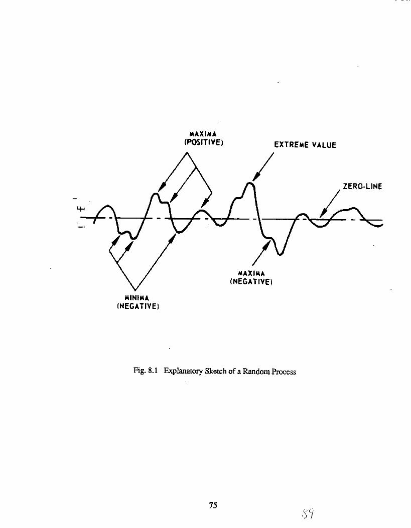
MAXIMA
(POSITIVE) EXTREME VALUE
MINIMA[NEGATIVE)
Fig. 8.1 Explanatory Sketch of a Random Process
75
8.2 Determination of Design Loads
Methods for the extrapolation of wave induced load were considered in the previous
section. In this section we consider how design loads are deii.ned. There essentially are
two possible criteria for the definition of design loads. These are to
a)
b)
Select the loads such that a certain level of exceedence is acceptable on the basis
of either short or long term procedures.
Select the loads such that the structural reliability level considering one or more
limit states is acceptable.
We illustrate the two procedures considering a stillwater load, a wave induced load and a
strength variable. The problem of treating combined loads for the same purpose of
identifying design loads is an advanced one, and is in fact part of a ship structure
committee research project on Load Combinations, SR-1337. Our more basic treatment
considers the stillwater lo~ wave load and strength to be independent of one another.
8.2.1 ~ ction of Maximum h ad Effect for Desi~
With a single wave load presen~ there is a one to one correspondence between the
load and the load effect In this context, the stillwater load is not speciilcally considered.
Because it is essentially constant over voyages that last days or a month, its inclusion or
consideration does not pose a difficult problem. The only question to be answered, then,
is how to determine the maximum expected wave load in the lifetime of the vessel. Such
load is pertinent to structural design for exrreme loads.
We previously described two methods for obtaining the distribution of the largest
wave load peak, either by using order statistics or by level crossing analysis. These two
classes of methods apply to a short term, i.e., seastate by seastate analysis. We also
described methods for the construction of the long term wave load distribution,
considering every load peak in each seastate. The following are the typical ways of
defining the extreme wave load for design, based on the above approaches:
T~
In design, the largest wave load is defined considering the most probable value of the
wave load distributions in each possible seastate. The number of short te.nn wave load
W* N is GO?ZlpUtdbill the ZeFOmtig Peti f~ edl *aS~t& ~ deSigll Wave
76q~

load is the largest among the set of short term most probable extreme wave loads for the
selected seastates.
The seastates should be selected on the basis of an acceptable return period and/or
acceptable probability of the ship encountetig such seastates. The latter depends on the
~~e~~=~ti~. R~erence [6]dmcribes tdmiques fur
computing probability of encountering a seastate of a speciiied return period, as well as
techniques for determining a seastate with a specified return period based on wave k
v Term Anal=
In this method, the design value is taken to be the largest wave load with an
exceedence probabfity of I/N, N being the total number of wave load peaks. In
calculating N, and in obtaining the long term distribution, each wave load peak possible
is considered. If the total number of load peaks is 108 in 20 years, for example, the
design value is the 108 exceedence level value from the long term distribution. This
value is said to occur once in the lifetime of the vessel.
While not usual, risk parameter can also be included in the long term approach. The
design value of the wave loa~ ~~, is then determined such that
where a is the risk parameter, e.g., 0.01, N is the total number of cycles (i.e., wave load
peaks) in the long term, and F(2Q is the cumulative distribution function of the long
term wave load.
8.2.2 ~~et Rellab@ ~vel. . .
Probabilistic methods provide a mechanism for obtaining extreme design loads for a
structure with the required target reliability or failure probability. The design safety
check equation for the limit state may take the conceptual form
o c~Y, D,+YwDw
where @is the strength partial safety factor, and y~and yWare the still water and wave
load partial safety factors. The C, D, and DWare characteristic values of the strength,
still water and wave loads. The seastate that defines DWwas previously identified. The
problem is then one of determiningg $, Y, imd YWconsidering the uncertainties in strength
77

and loads, such that a target reliability level is achieved. Level 1 reliability methods can
be used in this process. The derivation of the partial safety factors asstited with each
design variable, including the loads, for a target reliability level is described in Part 1 of
this report. For additional discussion of such procedures, the reader is referred to
Mansour [6].
78
9. Serviceability Limitstates
This chapter pertains to identii3cation and d~scription of important semiceabiIity limit
states. By definition, a seniceability limit state is associated with constraints on the
structure in terms of requirements such as maximum deflection of a member, critical
buckling loads that cause elastic buckling of a plate elemen~ or local cracking due to
fatigue. The limit state manifestations are typically of aesthetic, functional or
maintenance concern, but do not normally lead to overall edlapse. The following
sewieeabili~ limit states are now considered
(a) semiceability limit state associated with critical buckling stresses
(b) “Wmceab@limifstate awciatdwil.hfaligue
9.1 Serviceability Lhnit State for Plate Buckling
Plate elements in a ship hull, such as between longitudinal, can buckle under applied
loads in either the linear elastic or inelastic range of material behavior. A plate that
buckles in the linear elastic regime will essentially regain its original co@uration when
unloaded. C)nthe other han~ a plate that buckles in the inelastic regime may suffer some
permanent set upon unloading. The applied stress that defines the lower limit of the
inelastic regime is that corresponding to the material proportional limit. Thus the so-
called inelastic regime includes nonlinear elastic and plastic behavior.
Buckling of plate elements in the linear elastic regime is generally accepmble in
longitudinally tied vessel hulls, although it is rare that tie designer intentionally
designs the structure to behave so. The major exceptions to this occur in passenger
vess-els rurdcm-cmriem wherEthepIathrg cmdecksabow? theweathackck frvllTstmss
considerations alone can be relatively thin, their main function being to provide the
required weather and water-tightness. In such cases, it is efficient for the designer to
allow linear elastic plate buckling to occur, the result being a lighter structure than would
otherwise be the case, and also less topside weight.
Depending on the philosophy of the profession and the organizations, buckling of
plate elements in the inelastic regime may or may not be allowed, the primary
consideration being aesthetic. From a material utilization point of view, plate thicknesses
can be reduced if an amount of permanent set is allowed.
In discussing serviceability limit states involving plate buckling in longitudinally
framed vessels, the following nomenclature is adopted: The plate long dimension
79

(length) is assumed to be parallel to the x axis, or the vessel longitudinal direction, and is
labekxl “a”. The plate width or small dimension is taken parallel to the y axis or vessel
Iransvme direction, and is labeled “b”. The plate aspect ratio m is always lsrger than or
equal to unity. The plate thickness is denoted “t”. The plate element is considered under
uniform inplane compression, either in the longitudinal direction (the so-called long plate
case) cmin the transverse direction (the so-called wide plate case]. Another load case
considered is the plate under unif’ edge shesr. The semiceability limit state is reached
when the applied stress equals ~~ or 6P, where the limit c~ applies in the linear elastic
range, and GPapplies in the inelastic range.
IMform cQ~.
i
For long plate compression,
()ZZE t 2~m=k— -
12(1-v2) b
where k = 4 for simply supported edges. For other edge conditions, the buckling
coefficient K can be obtained horn the attached Figure 9.1. If cm s cm, the
P@ond limit,
Otherwise,
In the above, OYis the material yield strength.
For wide plate compression,
~m=k()
Z2E t 2
12(1-V2) ;
-( ~)where k - 1+ b2 z 2 for simply supported edges. If ams Um, the following applies.
ae=om.
80

otherwise,
The critical buckling stress is given by
()Z2E t 2%m=k— —
12(1-v2) b
()2
where k=5.34+4 ~a
for simply supported edges. If the edges can be considered clamped, the buckling
coefficient k takes the furtn
Otherwise, the limitstress is
where ~ is the shear yieId stress, etpil to crY@
The above solutions defining the serviceability limit states under uniform edge
compression or shear are based on classical buckling theory. Further reference is made
to [8]. The. limit stresses beyond the proportional limit are based on tangent modulus
corrections due to Bleich. The interested reader is referred to Bleich’s book on “Buckling
Strength of Metal Structures”, published by McGraw Hill, 1952. With a tangent modulus
correction q included, the limit stress can be written in the following form:
ap=k[)
rc2Eq t 2
12(1-vZ) ~
81

where q = f(E,Z), E, being the tangent modulus. The functional relationships defining q
are different for the long plate, wide plate and shear cases. Hence the corresponding CP
are also of different forms.
9.2 Serviceability Limit State for Fatigue
The fatigue limit state is associated with the damaging effect of repeated loadhg
which may lead to loss of a specific function, maintenance costs, and in certain cases to
ultimate collapse. That fatigue cracks in ships are more a maintenance than a safety
concern is essentially due to the ductility of ship steels. Fatigue cracks do occur in
complex structures, and design against fatigue (i.e., procedures to limit fatigue cracking
to acceptable levels) is important
Them are vtious possible ways of computing the fatigue damage in a vessel subject
to a speciikd long term wave environmen~ According to [61, the different methods may
be classilkd as those based on
(a) wave height history
(b) stress range history
(c) the entire scatter diagram
This mtxhod of classification, further explained in the attached Figure 9.2, is based on the
level of detail in tie treatment of the environment. Other types of classtication are also
possible, e.g., S-N cume based methods as opposed to fracture mechanics based methods,
design _ methods in cmrtrast to design checking rnethodsv and m on. The
fommlation of the fatigue limit state will depend on the details of the method used. In
this section, the formulation described is the one used in section 4.2.3 of this report.
The limit state formulation is based on S-N curves, which describe the number of
constant smplitude stress cycles to failure, as a function of the fluctuating stress
amplitude. The curve is written in the foxm
NASm=C
where N is the number of cycles to fsilure, AS is the constant amplitude stress range, and
m and C are slope and intercept related constants. For design purposes, C is chosen so
that the S-N cuwe forms a “lower bound” to the experimental data. One typical
statistical way of defining C is
82

logc=loge-2a=N
where ? corresponds to the median S-N tune, and clO~~ is the standard deviation of log
N. Each generic structural detail type has an S-N crtme. For a collection of S-N cumes
typical of ship structural detail situations, the reader is referred to Munse’s Ship Structure
Committee report SSC-318, “Fatigue Characterization of Fabricated Details for Design”.
The wave environment is described completely by the set of seastates and their
probabilities Qf ~ asdefine dinasmtterdi- Foreach seastateithemss
disrnbution can be considered Rayleigh distributed, assuming that the wave induced
siress prucess is narrow band and zero mean Gaussian. The Rayleigh density is of the
folm
where kOjis the zero moment of the stress spectrum in seastate ‘~”. ms moment is also
equal to the mean square value of the stms proms. The zero-crossing frequency of the
stress process in hertz (cycles/second) is given by
where ~j is the second moment of the stress spectrum for the seastate. If the time spent
h the seastate is Tpj$ where T is the total time period d pj is the probability of
occurrence of the seastate, the number of stress cycles associated with the seastate is
Also, the number of cycles associated with a stress interval ds is [f,(s)ds] . Tpj $
The fatigue damage associated with the seastate “j” can then be calculated using the
Miner linear cumulative damage hypothesis. The damage is given by
“’g (S$ds’
‘j= [ N,(AS)—Tpjfj
83 n

where N~AS) is the number of cycles to failure at the specified stress range AS as
Wermked fmm the S-N curve. %batitming for N#lS~ the above equation may be
rewriten as follows:
TPj ‘jy J Smf(S)dsDj=—co
Tpjfj
‘c (r I+m
T )
Here, the integral has been evaluated by substituting the Rayleigh density for f(s). From
this, and upon substituting for $ the total tige in time T, for j seastates, may be
obtained as
The above equation defines the fatigue damage from the entire scatter diagram, for
the time period T. If the Palmgren-Miner damage sum at failure is denoted 4, the time
to failure may then be obtained
Equation 4.5 of the text is directly obtainable from the above equation for time to failure.
That equation also includes a stress inaccuracy term B which represents the “modeling
emr” in the procedures used to compute the wave induced stress.
The above definition of the fatigue limit state equation in terms of the time to failure
assumes that the stress process within any seastate in the scatter diagram is narrow
banded. A comection for the possible wide banded nature of the process is available, see
Winching and Light, ASCE Journal of Structural Division, Vol. 106, No. ST7, July
1980. The wide band correction was derived by Wirsching and Light using rainflow
counting on simulated time histories of differing bandwidths to obtain the stress range
histogram and then computing the fatigue darnage, which then was compared to that
predicted from the narrow band assumption. The importance of the refinement obtained
84

by including the. correction is relatively small when compared to the inaccuracies
introduced by the stress modeling error in particular. Also, the come.ction assumes the
estimates obtained by a rainflow count based procedure to be the correct ones.
Nevertheless, the minflow cmrection provides a means for obtaining a fatigue damage
estimate that is somewhat more realistic than that calculated using the narrow band
assumptions. For typical stress time histories in ships, the effect of the comction is to
reduce the calculated damage.
85
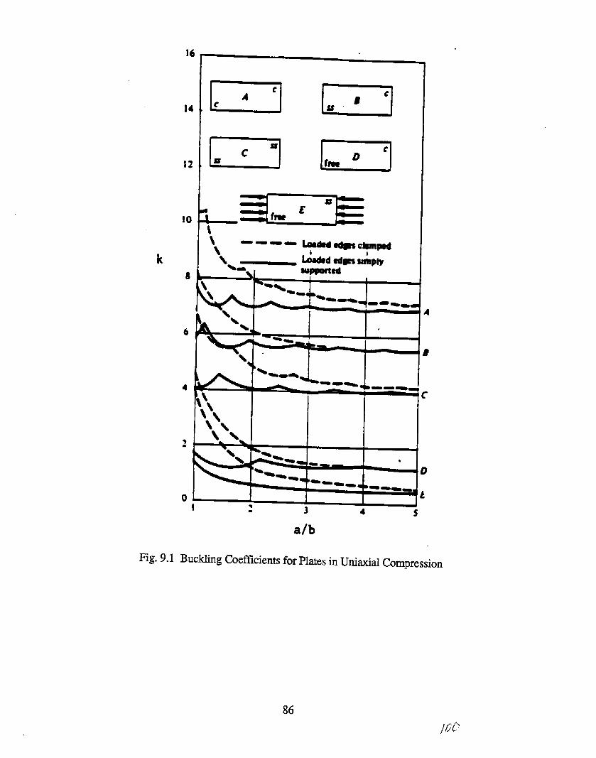
12
10
k8
b
4
0I
I
\ -\=l-
●
11 I 1. I
3
alb
4 s
Fig.9.l Buckling Coefficients for Plates in Utitial Compression
86
/00

SeastateDeflnftlon
1
7-=” -’1w
Have ExceecfanceHistogram (some-tfmcs called the“determfnistlc”method). ThisLechnique used lIyLloyd’s. Damagecomputed fromwave exceedanced!agram
I
IJ
Im
Iiave distributionmethod; stress assunedpm3po~tlonal to waveheight, and waveheight distributiondescrlbedby Iognonnal,tielbull, etc. tiolte-Hansfordmethdoassunes I#elbu?l distri-bution.
Stress Range Dfstrf-bution Method; stressrange model led theore-tically, usuallyWeibull. Stress rangedistribution can bederfved from spectralnethod, wave distri-.bution method, CLC.
Spectral Analysis(Based on a ful I scatter
diagrarndefinlng thelong term seastate)
I I
Spectral flethod(sometfmes calledthe “probabfllstfc”method]. Damagecomputed from eachseastate In scatterdiagram, In whichstress Is consider-ed a stationaryrandom process
The Equivalentkietbu?l Method:This method usedby flnV. Anequivant Melbu?ldlstrfbutlon oflong term stressranges is derivedusing spectralanalysis
Fig.9.2 ClassificationofFourBasicMethods ofComputingFatigueDamage

10. Limit States Associated with Lifetime Extreme Loads
The aim of this chapter is to identify and describe the appropriate limit states
asswtited with lifetime design extreme loads. The following global limit states are
considered:
(a) Hull girder initial yield limit state
(b) Hull girder fully plastic limit state
(c) Hull girder collapse limit state
The strength associated with the following local buckling limit states are also considerd
● Column and beam column buckling of longitudinal
. Torsional/flexural buckling (tripping) of longitudinal
o Grillage buckling of longitudinal together with transverse beams
The global limit states apply to the hull girder as a whole. The local limit states
apply to portions of the hull girder, e.g., longitudinal between transverses, longitudinal
and associated flange plating between transverses, or gross panels consisting of. .
hgmdmds andtrarrsvmses. 14atebncHing p’asei’s noteonsidm@mcept to the
extent it reduces the effective flange plate acting together with the longitudinal.
Global and local behavior are interlink~ and an argument may be made that
consideration of global behavior alone is sufficient provided the consideration is detailed
enough. Nevertheless, a two level approach is used because
(a) Separate consideration of local behavior affords the designer more control over
material deployment.
(b) Local behavior is often indicative of global behavior.
(c) A two level limit state design procedure is more consistent with present
conventional design practice.
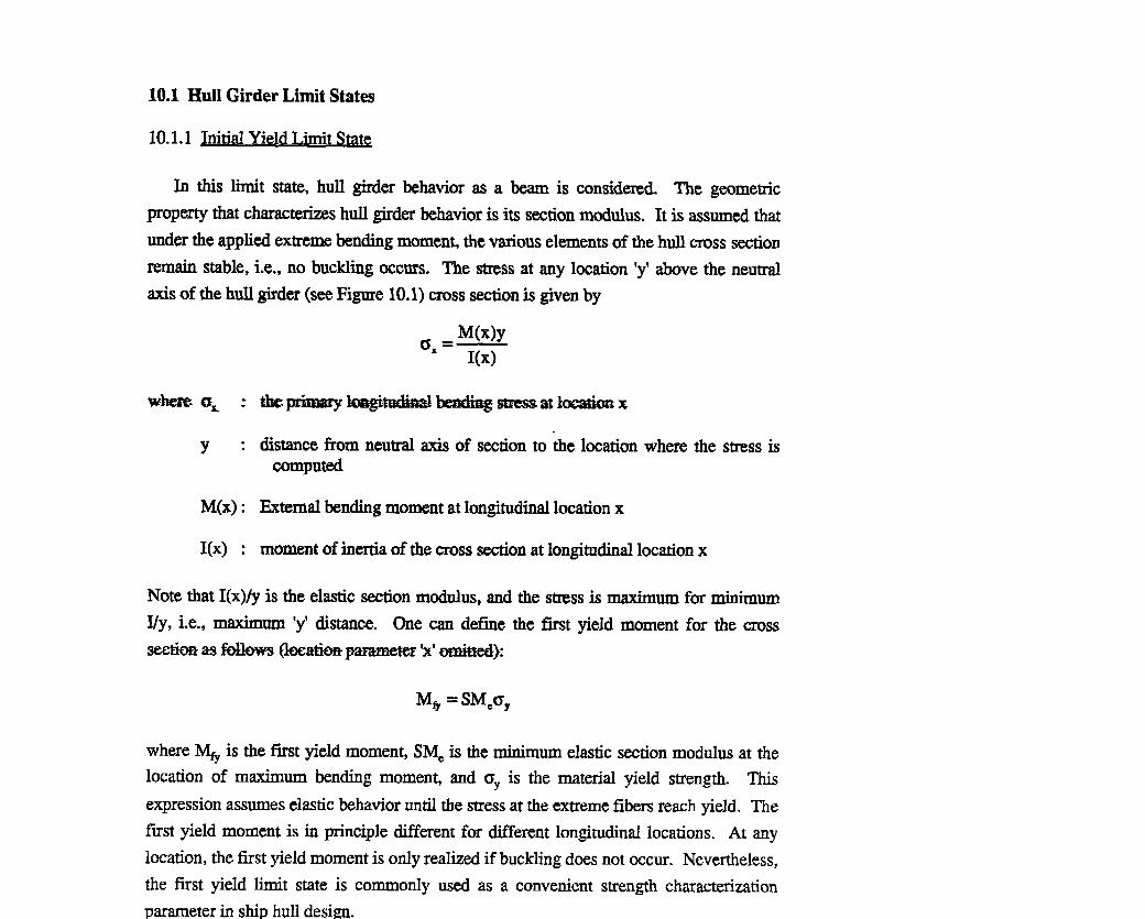
10.1 Hull Girder Limit States
10.1.1 JnitialYield Limit State
In this limit state, hull girder behavior as a beam is considered. The geometric
property that characterizeshull girderbehatior is its section modulus. It is assumed that
underthe applied extreme bending momen~ the various elements of the hull moss section
remain stable, i.e., no buckling occurs. The stress at any location ‘y’above the neutral
axis of the hull girder (see Figure 10.1) cross section is given by
~ = M(x)yx
I(x)
where ax :
Y:
M(x) :
I(x) :
the-bq@udiAk&mdiEg-#~x
distance from neutral axis of section to the location where the stress iscomputed
External bending moment at longitudinal location x
moment of inertia of the moss section at longitudinal location x
Note that I(x)/y is the elastic section modulus, and the stress is maximum for minimum
IJy, i.e., maximum ‘y’ distance. One can define the ftrst yield moment for the cross
section as follews (hmtionprameter ‘x’omitted}
M& = SMeoY
where ~ is the fit yield momen~ S% is the minimum elastic section modulus at the
location of maximum bending moment, and OYis the material yield strength. This
expression assumes elastic behavior until the stress at the extreme fibers reach yield. The
frost yield moment is in principle different for different longitudinal locations. At any
location, the first yield moment is only realized if buckling does not occur. Nevertheless,
the fust yield limit state is commonly used as a convenient strength characterization
parameter in ship hull design.
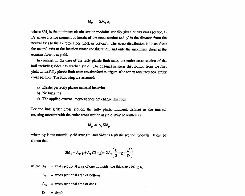
M@ = SM+
where SW is the minimum elastic section modulus, usually given at any cross section as
I/y where I is the moment of inertia of the cross section and ‘y’is the distance from the
neutral axis to the extreme fiber (deck or bottom). The stress distribution is linear from
the neutral axis to the location under consideration, and only the maximum stress at the
extreme fiber is at yiel~
In contrast in the case of the fully plastic limit state, the entire cross section of the
hull including sides has reached yield. The changes in stress distribution from the first
xto&~_M==~k_ifi~ 3a2f~~=ztiti~
moss section. The following am assumwl
a)
b)
c)
Elastic perfectly plastic material behavior
No buckling
The applied external moment does not change direction
For the box girder cross section, the fidly plastic momen~ defined
resisting moment with the entire cross section at yield, maybe written as
as the internal
where q is the material yield strength, and SMp is a plastic section modulus. It can be
shown that
SMP =AD g+ A~(D-g)+2A~();-g+$
where As = cross sectional area of one hull side, the thickness being ~
A~ = cross sectional areaof bottom
AD = cross sectional area of deck
D = depth
&AB+2A~-AD
D - 4A,
For mm compkated moss sections andlim if more than one material is used in the
hull cross section, the fully plastic moment needs to be numerically calculated, i.e., close
form solutions such as that for the box girder are not available.
In general, the fully plastic limit state is not useful in a practical sense as the physical
condition it represents is seldom realized because of buckling. It has been historically
used, however, as a baseline value to which a buckling knockdown factor was applied in
order to obtain the collapse moment for the hull cross section, particularly if the cross
section is multicellular. For unicellular cross sections, a more appropriate baseline value
is given by the first yield moment In current practice, the buckling knockdown factor is
applied to the initial yield moment as indicated in Part 2 of this report.
The fust yield limit state and the fully plastic limit state are both idealizations of hull
girder behavior. In reality, as the external.1~ applied curuature @ moment) on the hull
girder is increased, strains internally will inmease up to a point where either the yield
strength of the material is reache~ or buckling occurs depending on the slenderness of
the structure. Of particular importance in longitudinally framed vessels is the buckling
and post buckling behavior of longitudinal together with asswiated plating, and also in
some cases the overall buckling of the gross panel consisting of longitudinal together
with the transverse beams. When parts of the hull buckle, any additional load is “shed”
to or taken by adjacent stable material, up to the point at which they also buckle or reach
yield. As the externally applied cumature increases, typically the internal resisting
moment calculated with accounting of buckling and yielding in parts of the cross section
wiU increase up to a point, after which it will drop. The maximum internal resisting
moment so calculated is the so-called collapse moment, !MC’.on the tension side of the
hull girder, the unloading,lload shedding is slower and on the compression side, it is more
rapid A typical moment-cmature diagram for a hull cross section is illustrated in
transversely framed situations, the plate effect on collapse moment is comparatively
greater*
of c’—’—
There are various possible methods for calculating the collapse moment. These vary
from approaches where any reserve of stiffened plate compressive strength after its
maximum resistance has been reached is neglected, to nonlinear finite element
calculations which include pla.stification and buckling in a rigorous way. The concept of
dmvnrating or knocking down the fully plastic collapse moment to account for buckling
was suggested by Caldwell [16J. It has been further developed by Mansour [7], but with
knock down factors to be applied to the initial yield momenk Procedures incorporating
an inmemental moment-cumature approach to hull collapse strength have been developed
by Smith, Billingsley [17] and Adamchak [18]. Finite element calculations for ship hull
collapse strength are presented in Thayamballi et al. [19].
It is not the intention to review the different methodologies for ship hti collapse
strength calculation, but we imoduce in brief here, the incremental moment creature
approach. In this method
(i) A cumatureis applied to the hull, and increased incrementally.
(ii) For each value of mature, the internal resisting moment is computed,
accounting for the end shortening of the element resulting from internal
stmi.ns, including any buckling and post buckling, as wtdl as load limitation by
plasticity. Such information is included through load-end shortending ctuves,
an example of which is shown in Figure 10.4.
(iii) A moment cumature relationship for the hull, such as that in Figure 10.3, is
developed, and the collapse moment idendfled.
The most important part of the calculations is the establishment of the load-end
shortening relationships for the hull members, considering the various local failure
modes.
10.2 Limit Statm Associated with Local Buckling
10.2.1 Gener~
Aprevio@y nQte,&*-t&wqr@ ~ Withmlumnardkcolumn buckling of longitudinal together with asswiated plating, tripping of
longitudi.mds, and the grillage buckling of longitudimils together with transverse beams.
The strengths calculated do not account for any post buckling reseme which is typical
small (but existent) in the failure modes noted. Also, the term “local” is used as a
qualiiier to the extent that only one component is considered in the limit state. In the real
structure, here may be several such identical components under nominally identical
loading.
10.2.2 Column and Beam Column Buckling
Column buckling refers to the flexu.ral buckling of longitutials together with
effecting plating. The longitudinal and plating may be part of a stiffened panel between
transverse beams. The panel, and hence the longitudinal and plating are considered to be
under compression. k the beam-column failure mode, in addition to the axial load, there
are also lateral loads present. This latter situation occurs for example in the case of
longitudinal and plating at the vessel bottom. The column idealization is shown in
Figure 10.5.
Column buckling strength, without consideration of lateral pressure, is given by the
following (Mansour, Ref. 8):
acr = (1:)’

The frost equation, valid in the range of O s am S OP,where OPis the proportional
limit stress and mfi is the critical buckling stress, will be recognized as the Euler elastic
column strength equation. In the second equation, a correction is made, based on a factor
Cs, if the calculated elastic buckling stress exceeds the proportional limit stress aP The
correction is such that the limit state strength calculated horn the pair of equations given
will not exceed the material yield strength.
Also, ‘l.’ is the effective column length, which in continuous structures where the
stiffener ends are capable of rotation, may be taken equal to the physical length between
transverse supports, and ‘r’ is the radius of gyration of the cross section consisting of
plating and stiffener. The value of r is given by:
where ~ and ~ am the moment of inertia and - of&e cross sect.kml IW&ti%’dy.
Typically, in computing these quantities, an effective plate flange assuming that the plate
has buckled is used. The plate flange width may be obtained, for short edge
compression, from IWnsour, Ref. 8, as follows:
b 1.9~=_b P
2.25 L25—.—‘PB2
1.0< p <3.5
= 1.0 psl
where ~ is the non-dimensional plate slenderness, defied as:
1? q?d=——t E
where b is the width of the short edge, i.e., the spacing of Iongitudinals.
In the case of beam-column buckling, the lateral pressure results in a reduction in the
critical stress to a value less than that obtained for the column buckling limit state. A
94
relatively simple approach to characterizing limit state strength for this situation is to use
a linear interaction equation.
0= a~—+— =1am ay
where e= is the column buckling strwq$h assuming m kMeralpressure, and 6Y is the
yield strength. aa is the axial stress and ~ is the maximum bending stress over the span
of the longitudinal. This interaction equation assumes that tripping of the moss section,
and local buckling in the moss section (e.g., of the flange or web) are avoided.
The calculation of a, should account for any reduction in plate effectiveness because
of buckling. The calculation of the
lag effects, although fur panels with
neglecti
bending stress should in principle account for shear
closely spaced longitudinal, the effect may often be
In this failure mode, also called torsional/flexural buckling, failure is initiated by
-gdti~h tia~titie ~~k-mmdplmk
not move laterally. A portion of the adjacent plate may participate in the twisting, and
the flange of the stiffener may twist together with the web, or the two may twist
differentially. Tripping is illustrated in Figure 10.5. The tripping phenomenon may
occur under axial loads alone, or under axial loads in combination with lateral pressure
loads.
The ultimate strength for torsional/flexural buckling under axial compressive loading
may be obtained as follows (see Reference 8):
a) Calculate the elastic tripping stress q for the stiffener cross section rotating about
an enforced axis at its toe. This is given by
‘t=;@+*)
where G k. the Shm mmhdus. fm tk. rnateria~ J is the torsion constant, and Cwis.
the warping constant. The length of the longitudinal between supports is denoted
‘1’. Expressions for the torsion and warping constants as a function of cross
95

b)
section shape may be found in the book by Bleich, Ref. 20. ~ is the polar
moment of ineltia of the cross section about an enforced axis at its toe, i.e.,
10= IX+~+Ay2
where ~ and ~ are the principal moments of inertia of the cross section, of area
A, and y is the web depth.
Obtain the elastic tripping stress atiC considering interaction with column
buckling, by solving the following quadratic:
Here, ICis the polar moment of inertia of the cross section of the stiffener, i.e., ~
+ ~, and axis the limit state strength for column buckling under axial loads. If
atfe < OP,where UPis the proportional limit stress, the tripping knit stress Oti=
ode. Otherwise, atfis obtained from
The above determination of limit state strength for tipping of longitudinal under
axial loads is outlined in Mansour, Ref. 8. When lateral pressure is present, the axial
tripping strength should be modified to reflect its influence. Although more detailed
approaches are possible, one way to include the lateral pressure effects is to use a linear
interaction formula similar to that used for the case of the beam-column limit state. Such
an approach will not apply to a case where the pressure loads are the dominant ones, and
additional refinements will be needed.
10.2.4 Grilla~e Buckling
This failure mode and the limit state strength associated with it refer to the buckling
of the gross panel, i.e., longitudinal and transverses, between the major support
96@
members such as bulkheads. A portion of such a gross panel under compression is
shown in Figure 10.5. This problem has been extensively studied by Mansour [21,22]
using orthotropic plate theory. The following, taken from Ref. 22, may be used if the
number of stiffeners in each direction is sufficiently large, e.g., 3 to 5.
For gross panels under uniaxial compression, the critical buckling stress is given from
where B is the width of the gross panel, lq is the effective thiclmess resisting
compressive loads in the x direction, and k is a buckling coefilcient that depends on
boundary conditions. For simply supported gross panels,
the
the
For gross panels with both loaded edges simply supported and both the other edges freed,
m’ 2k= —+2.5q+5~
P2
where m is the number of half waves of the buckled orthotropic plate, to be chosen such
that k is minimizem q and p are the virtual aspect ratio and the torsion coei%cient,
respectively.
The.vktualasp.ectratio mdthemioncoeff* megivmby
r
1P 1Pn
‘~
r
L D,
“E 4~
Here (see Figure 10.6), DXand DYare the flexural rigidities per unit width, given by
‘x=% ; “=&
97
where ~ and ~ are the moments of inertia of the stiffeners extending in the x and y
directions (i.e., about the y, x axes), and IPX,IPYare the moments of inertia of the
effective plate flange alone, acting with the stiffeners in the x, y directions. SXand SYare
the x and y stiffener spacings.
The effective plate thickness
effective plating and stiffeners in
~ is the average cross sectional area per unit width of
the x direction, i.e.
hX=A,+Sct
s,
where As is the stiffener area, t is the plate thickness, and Se is the effective width of the
plate flange, S, S SY.
Reference 21 by Mansour contains an extensive treatment of the behavior of
orthotropic plate panels in the buckling and elastic post buckling range. Design chats
are given, which address, for example, the midplane deflection, critical buckling stress,
and the bending moment at midlength of the edge. The types of loading considered
include combinations of normal pressure, direct inplane stresses in two directions, and
edge shear stress. From the charts, prediction of large deflection behavior up to the onset
of yielding is possible in a practical sense. Alternatively, in a unidirectional load
situation which is a very common case, limit state strength may be obtained from the
previously given close form expressions from Ref. 22. That solution is not valid beyond
the linear elastic regime, unless confections of the type made for column behavior are
also made in this case.
98
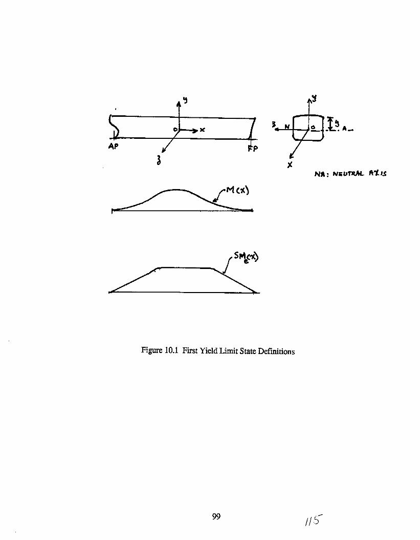
Figure 10.1 First Yield Limit State Deftitions
99
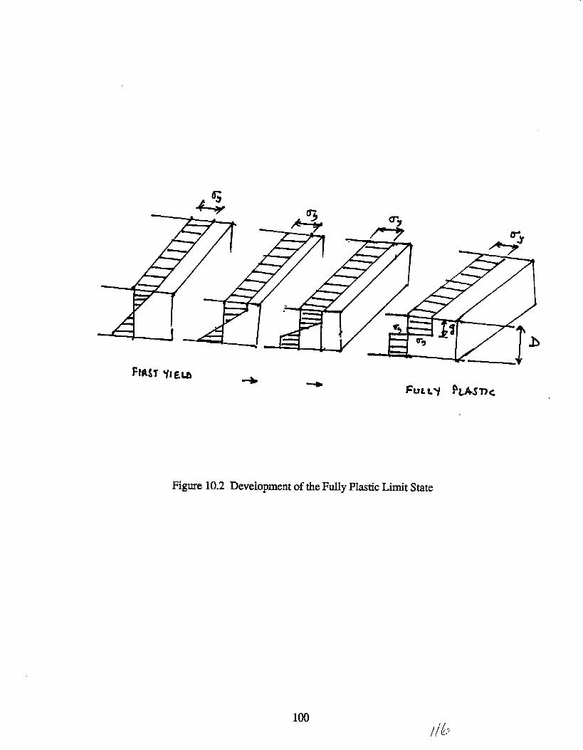
m J= -r”:#
/7-/ 257”-e.“u
Figure 10.2 Development of the Fully Plastic Limit State
100

--—
M’ltrrnf U*M W&
Figure 10.3 Moment-Cuature Diagrams for a Ship Hull
101

IP..
Figure 10.4 Load-End Shortening Curve for a Column
102 /,r

—
Figure 10.5 Stiffener Plate Failure Modes
103,

r x
i
I [ [’ I J i
Figure 10.6 Definition Sketch for Gross Panel Buckling
11. Conclusions and Discussion
11,1 Summary and Major Results
Two demonstrations have been cnrried out in this projec~ a demonstration of
probability-based Rule calibration (Part 1),.and a demonstration of probability-based, hull
girder safety analysis (Part 2). Also, an ‘extension to the projec~ Part 3 defined loads,
strength and structural reliability terminology, identified ultimate and serviceability limit
states, and considered procedures for IGadextrapolation and load definition. ,-
In the first part, the calibration procedure was described and applied to ABS hull
girder longitudinal strength formulation. For this purpose 300 “ABS Ships” are
considered and the minimum required section modulus of each hm been determined
according to ABS Rules (see Appendices 1 and 2). The safety index ~ was then
determined using first and second order reliability methods. It was found that the safety
indices vary slightly and that variation depended only cm the ratio of the wnve bending
moment to the sti]]water bending moment. The range of the safety indices, &lllge=&nax-
~n~., was found to be 0.31. The average value of the safety indices [~nvwas found to be
3.2.
The aim of the calibration procedure, which “is described in detail in Pnrt 1 of the
report, is to eliminate this variation in ~ in order to achieve uniform safety standard for
all ship sizes. The target p value was. taken ns the average value,pl=~av=s.z. The
calibrated formulation, which is bnsed on Pm_tinlsafety factor format, produced the target
value of ~ nnd n f!~nge=0.004.
It should be noted that the cnlibratecl formulation, in m much m the initial ABS
formulation, ensures only a safety level agninst deck yielding. For buckling
considerations, the stiffening system for each of the 300 “ABS Ships” must be designed
and evaluated. Buckling rule calibration is best done at the local level since the Rules
control and specify stiffener spacing, section modulus and plate thickness at a local level.
Similm calibration procedure to that described in Part 1 can be used to calibrate ABS
formulations thnt give minimum required stiffener section modulus nnd plate thickness so
as to produce uniform safety.
In Part 2 of the report a tanker was tnken m an example to demonstmte the use of
probability-based safety rmalysis, i.e., to estimate the reli:lhility in an existing ship (or on
a drawing board design). For this purpose several limit states have been developed
including ultimate strength (buckling collapse, deck initial yield and fully plastic
collapse), serviceability limit state (local plate buckling) and fatigue limit state. More
1 o~

. .— .. ,.
realistic load estimates have been developed for each lim,it state, based on parametric
seakeeping and ship motion analysis. The wave bending moment has been calculated for
the ultimate limit sklte with considerations given to the most probnble extreme sea
condition the ship is likely to encounter. For the fntigue limit state, stress ranges and
number of cycles have been calculated b~ed cmn sea scatter diagram.
A reliability, index @ has been:,calcallated u)ing, ~i~t,,and. second order reliability. ... . ..... ... ... . . . .methods for each limit state. Model, &certainty was included in all limit states. The
resulting safety indices indicate that bticklin”gcol lapse is the “governing mode of failure as
its safet y“index ‘iswell below those of deck~bitial<yi;ld and filly ‘plastic collapse.
11.2 Benetlts and Drawbacks of Using Probability-based Design Method
Use of probabilistic methods in design cim provide seveml benefits nnd some unique
features. Among those are:
1. Explicit consideration and evaluation of uncertainties associated with the design
variables.
2. Inclusion of all available relevant info~~tion in,the design process.
3. Provides a framework of sensitivity rne~sures.. ,.
4. Prcwides means for decomposition of global safety of a structure into partial safety
factors associated with the individual design variables.
5. Provides means for achieving uniformity of safety within a given class of structures
(or specified nonuniformity ).
6. Minimum ambiguity when updating design criterifi,
7. Provides means to weigh variables in terms of their significance.
8. Provides rationale for data gathering.
9. Provides guidance in novel design.
10. Provide the potential to reduce weight without loss of reliability, m improve
reliability without increasing weight. The methods can identify and correct overly
and unduly consewative designs.
106
-—- “,
.. ...
In addition to the above benefits, reliability technology lends itself for certain use for
which it is much more suitable than traditional design methods. In reference[14],
Wirsching lists some of its use, which include:●
1. To compme alternative designs, pm-titularly in the early stages when several
competing design concepp ,are Cons,idefid.. ,.,2. To perform failure analysis of a component or a system.
3. To develop a &ategy for design and maintenance of structures which age (e.g.,
corrosion, fatigue), and to determine inspection intervals.
4. To execute “economic value analysis” or “risk based economics” to produce a design
with a minimum life cycle cost,,.
5. To develop a stmtegy for design, warranties, spree pmh requirements.
6. In general, as a design tool to mnnng,euncertainty in engineering pmhlems.
Use and implementation of probabilistic methods nre not without problems. Some of
the drawbacks are:
1. Use of reliability analysis in safety and design processes requires more information on
the environment, loads and the properties and characteristics of the structure than typical
deterministic analyses. Often some information me not available or may require
considerable time and effort to collect. Time and schedule restrictions on design are
usually limiting factors on the use of such methods.
2. Appliciition of probabilistic and relinhi!ity methods usually require some familiarity of
basic concepts in probability, reliability and statistics. Practitioners and designers are
gaining such familiarity through seminars, symposia and special courses. Educational
institutions are also requiring more prrhbility and statistics courses to be taken by
studen~s it the graduate and undergraduate levels. This, however, is a slow process that
will take some time in order to produce the necessary “infrastructure” for a routine use of
reliability and probribilistic methods in design.
3. On a more technicnl aspect, the reliability ilnnlysis did not deliver what it initially
promised, that is, a true measure of the reliability of a structure by a “true and actual”
probability of failure. Instead what it delivered is “notional probabilities” of failure and
10?
/,2 3

._=. -- - ---- . . .-. ... ..
safety indices which are good cm1y as compamtive measures. Only notional values are
delivered becmse of the many assumptions ml approximations made in the analysis
producing such probabilities and indices. These approximations, deficiencies and
assumptions, however are made, not only in probability-based design, but also in
traditional design. Approximations are made in the determination of loads using
hydrodynamics theory and in the structural rmalysis and. response to the applied loads..,,,. ,. ,., . . ... .. .. ....... ..,,-,..When all such assumptions and deficiencies are removed from the design analysis, the
resulting probabilities of failure will approach the “true” probabilities.,.. . ,. ,-. ,’
11.3 Discussion of SSC Project% in Reliability and Needs to be addressed in
Further Pro,jects
The strategic plan of the Committee on Marine Structures (CMS) m outlined in the
Marine Board report “entitled “Marine Structures--Research Recommendations for FY
1992” has been reviewed. In this document, the CMS states the goals and objectives of
the plan and lists a five-year research program and development which is organized,.
under five technology areas. The technology areas are: reliability, loads and response,
material criteria, fabrication and maintenance, and design methods. The five technology
areas consist of 23 comprehensive and well thought-out subject areas. The projects
outlined in these subject arens will undoubtedly lead townrds fulfilling the goals of the
plan which include improving the safety rind integrity of marine structures, improving
competitiveness of U.S. merchant shipping, and promoting the development of new
marine systems.
Based on the work carried out in this project and the revi~w of CMS research
recommendations, the following areas are suggested for further development. Some of
these areas are very specific and each need to he addressed in depth m a limited scope
project. These ~Ips are:
1. Torsionrd/flexural buckling (tripping failure) of ship stiffeners with effective breadth
of plating -- analysis and development of design formulation.
2, Ultimate strength of ship hull girders due to instability -- mmlysis to determine
strength reduction factors due to instahi Iity tn be used in design,
108
.:-”.- _.
3.
4.
. .
Experiments on hull girder ultimate. strength to verify mxdytically calculated strength
reduction factors.
Selection of wave spectra (or wave data) pertinent to design wave loading on ships.
..-...—-.. .
.,. .,.”
,-
,.,,.:-,,..,,:, . ..... ...”..,. .“””.... ..
5. A study leading to the;determiriation of theratio sag to hog wave bending’ moments,--- .:,....
and the bias associated “withIine.ar.ship motion load prediction. ,.,,, ,..,. ..,. ... .. ..~.,,... .... . ....... . . . ,, ,., . . .
6. Design formulation for combined wave and slamming bending moments.
7. A study of shear forces and moments acting on the fonvard part of a ship including
slamming effects.
8. A study leading to target reliabilities for each hull girder limit state based on existing
ships.
9. Development of reliability procedures and target indices for local structure in ships.
10. A study to develop a,ielihbility-bnsed. cost nnqlysis which aims to nchieve minimum
life cycle costs for ships.
11. Development of a reliability-based strategy for inspection intervals and maintenance
of ships.
12. Inclusion of system reliability considerations in fatigue and multiple failure. modes.
13. Reliability assessment of transverse structures and lateral pressure efi%c~s.
.
109 /,.J.5’

ACKNOWLEDGEMENT
This project has been supported by the Ship Structures Committee. The
authors would like to thank the Project Technical Committee and its chairman, Mr.
Norman Hammer for their advice and suggestions during the project work. Sincere
thanks are expressed to Dr. James Lloyd, Exxon Productions Research Co., for the
information he provided on the calibration procedures used in API guides.
109a

12. References
1. ABS Report to the Technical Committee,’’Proposed Change to Rules for Building and
Classing Steel Vessels”, American Bureau of Shipping, September, 1990
2. “Rules for Building and Classing Steel Vessels”, Americm Bureau of Shipping 1990
3. Sowes, C.G. and Moan, T., “Statistical Amdysis of Stillwater Load EffecL~in Ship
Structures”, SNAME. Trans., Vol. 96, 1988
4. Mansour, A.E., “Extreme Vrdue Distributions of Wave Loads and their Appli&~ticmto
Marine Structures”, ~
Arlington, Virginia,0ctober,1987
5. Liu, P-L., Lin, H-Z., and Kiureghian, A.D., “CALREL User’s Manual”, Technical
Report UCB/SEMM-89/18, Department of Civil Engineering, Univemity of
Gllifornin, Berkeley, )989
6. Mansour, A.E., “An Introduction to Structuml Reliability Theory”, Ship Structure
Committee Report, SSC-351, December, 199(I
7. IMnnsour,A.E. nnd Thaylmhalli, A.,’’Ultimnte Strength of n Ship’s Hull Girder in
Plastic and Buckling Modes”, Shi~ Structure Committee Report, SSC-299, July, 1980
8, Mansour, A.E., “Approxim:lte Formukw for Preliminary Design of Stiffened Plates”,
Proceedings. Fifth lnterrmtional Svmwsium :ind Exhibition on Offshore Mechani~
and Arctic Entzineerin~ Tokyo, Japan, April, 1986, pp.427-434
9. Proceedimzs of the 11th lSSC, Remrt of Committee. Vol. 1, “Applied Design”, Wuxi,
China, 1991
10. Wirsching, P.H.”ilndChen, Y.N., “Fatigue Design Criteria for TLP Tendons”, Journal
of Structural Engineering, 113(7), July, 1987
11. Ximenes, Marin Celia C., “System F;ltigue Relinbiiity: A Stu~iyof Tension Leg
Platform Tendon System”, Ph.D. Dissertation, Navnl Architecture nnd Offshore
Engineering Department, University of Californi~\, Berkeley, Novemlwr, 1990
12. Loukrikis, T.A. and Chryssostornidis, C., “Seakeeping Series for Cruiser-Stern
Ships”, SNAME, Trnns., 1975
13. Gurney, T.R., “Fatigue of Welded Structures”, Cambridge University Press, 1979
14. Privnte Communication with P.H. Wirsching d:~tedNovember 26, 1991
15. Steel, R.G.D. and Torrie, J. H., “Principles }]ndProcedures of Statistics”, McGraw
Hill, New York, 1980
16. Caldwell, J.B. (1965) “Ultimate Longitudinal Strength”, Trmm. RINA, 1965
17. Billingsley, D. (1 980), “HullGirder Response to Extreme Bending Momen~%”,Proc.,
SNAME STAR Symposium, Cmomdo, CA 1980
110

18. Adamchak,J.C.(1982), “ULTSTR: A Pmgrnm for Estimating the Collapse Moment
of a Ship’s Hull Girder Longitudinal Bending”, DTNSRDC Report, October 1982
19. T1-myambnlli,A.K., Kutt, L.M. and Chen, Y.N. (1986) “Advanced Strength and
Structural Reliability Assessment of the Ship’s Hull Girder”, Proc. Sympnsium on
Advances in Marine Structures”, Admirnlty Resenrch lZs~~blishment,Elsevier Applied
Science Publishers, London, 1986
20. Bleich,F.(1952) “Buckling Strength and Metnl Structures” McGraw Hill
21. Mansour, A. (1976) “CharLsfor the Postbuckling Analysis of Stiffened Plntes under
Combined Loads” SNAME T&R Bulletin 2-22, July 1976
22. ManSour, A. (1977) “Gross Panel Strength under Combined Loading” Ship Structure
Committee Report SSC-270, 1977
111
APPENDIX1
MSW, Mw, Mw/Msw, and SM of “ABS Ships”
1-1
-.
,;..,’: .:, ,:,,...,,, .,, ,,. .:.,,:.. .. , .,’. ,, ,:,,, ,
,, .. . .. ... . . ,, ..: ,:, ,,, .,
L (m) L/B91.5 5.091.5 5.091,5 5.091.5 5.091.5 5.091.5 5.091.5 6.091.5 6.0
~+ 91.5 6.091.5 6.0
,’ 91.5 6.0‘]91.5 6.0,—. 91.5 7.0
91.5 7.0“k-”-91.5 7.0
91.5 7.091.5 7.091.5 7.091.5 6.091.5 e.o91.5 S.o91.5 C+.o91.5 S.o91.5 a.o91.5 9.091.5 9.091.5 9.091.5 9.091.5 9.0
+91.5 9.0‘122.0 5.0i~122.0 5.0122.0 5.0122.0 5.0122.0 5.0122.0 5.0122.0 6.0122.0 6.0122.0 6.0122.0 6.0122.0 6.0122.0 6.0122.0 7.0122.0 7.0
- 122.0 7.0lu~zz.o 7,0
:M122.O 7.0122.0 7.0122.0 0.0122.0 a.o122.0 e.o122.0 e.o122.0 8.0122.0 B.o122.0 9.0122.0 9.0122.0 9.0122.0 9.0122.0 9.0122.0 9.0152.5 5.0152.5 5,0152.5 5.0
Cb0.600.650.700.750.800.850.600.650.700.75o.aoo.a50.600.650.’700.750.60o.a50.600.650.700.750.000.s50.600.650.700.750.600.650.600.650.700.750.80o.a50.600.650.700.750.800.850.600.650.700.750.800.1150.600,650.700.750.80O.es0.600.650.700.75O.ao0.850.600.650.70
Msw (kN-m]104026.36700lo8754.02aool134a3.31300lla211 .77300122940.23400127660.72700B66B8.6406090629.0234094569.429709a509.81250
102450.19500106390.6020074304.5469077682.0234081059.50700B4436.9a44087014.4531091191.9453065016. 4a05067971.7656070927.0703073aa2.3594076a37,64E14079792.9531057792.4258060419.3477063046.2052065673.210906B300.1328070927.07030
261790. 6a800273690.25000285509.84400297489.406003093a e.969003212 Ba.56300218159.90600226075.20300237991.53100247907.84400257S24.15600267740.46900186993.35900195493.03100203992.73400212492.43800220992.12500229491.414400163619 .lBaOO171056.40600170493.64100le5930.e7500193360.10900200005.35900145439.20100152050.1410015B661,01600165271 .a9100171002,76600170493.65600540497 .6aBoo565065.750005B9633. U1300
Mu (kN-m)169564.21900176085.90600la2607.62500109129.34400195651.03100202172.71900141303.51600146738.26600152173.03100157607.78100163042.5310016a4??.26600121117.30500125775.65600130434.02300135092 .391ao13975a.73400144409 .a9400lo5977.641aolloo53.695aa114129.766001182a5. a44ao122261 .B9800126357 .953ao94202.3437097825.50700
101448.60000lo5071. a590010a69S.01600112316.18000434950.56300451679.3750046!340e.2aloo4a5137.21900501a66.0310051!1594.8750036245a.-lfJloo376399 .5aaoo390340.219004a42e1.000oo418221 .6BSO0432162.3750031067 B.969OO322628.12500334577.34400346526.56300358475.75000370424.90600271844.094002a2299.62500292755.15600303210.75000313666 .2E1OO324121 .7B1OO241639.20300250932 .9a40a260226.81300269520.65600270014.469002I3U1OO.25OOO900691 .60S00943641.3130097e591.000oo
HM4au1.630011.619111.6a9111.599921.591431.5a3571.630011.619111.609111.599921.591431.5s3s71.630011.619111.609111.599921.591431.583571.630011.619111.609111.599921.591431.583571.630011.619111.609111.599921.591431.583571.661441.650331.640141.630771.622121.614111.661441.650331.640141.630771.622121.614111.661441.650331.640141.630771.622121.614111.661441.650331.640141.630771.622121.614111.661441.650331.640141.630711.622121.614111.6a1211,6699?1.65966
SM {m-cm-m)15414.9297016007.6106016600.6934017193.57620177a6.457001B379.3399012845 .’7744013339 .642ao13U33.9111O14327.9005014a22.0479015316.1162011010.6641011434.15040llo57.63a7012201.1260012704.612301312a .099609634.33105
looo4. aaleo10375.43360lo745.9a54a11116.53610114a7. oa690$563.049610893 .228S19222.607429551.9073098B1.36523
10210.7441039540.9570041061.7617042582.5703044103.3709045624.1797047144.9083032950.7969034218.1367035485.4727036752 .a164036020.15240392U7.4e8302L3243.541OO29329 .S301030416.1211031502.4121032588.7012033674.9922024713.0977025663.6016026614.1055027564.6113028515.1133029465.6172021967.1973022e12.oa99023656.9824024501 .S770025346 .76?6026191.66020a2600.33590e57a5.5wloaa962.02alo
L(m)152.5152.5152.5152.5152.S152.5152.5152.5152.5152.5152.5152.5152.5152.5152.5152.5152.5152.51S2.5152.5152.5152.5152.5152.5152.5152.5152.51413.Ola3.o103.0103.0163.0163.0183.0la3.o183.0103.0183.0la3.o103.0le3.o183.0183.0193.0103.0103.0183.0163.0la3.ole3.o103.0103.0183.0183.0103.0163.0183.0213.5213.5213.5213.5213.5213.5
L/B5.05.05.06.06.06.06.06.06.07.07.07.07.07.07.08.0a.o6.00.08.0a.o9.09.09.09.09.09.05.05.05.05.05.05.06.06.06.06.06.06.07.07,07.07.07.07.0a.o8.00.0a.oa.oa,o9,09.09.09.09.09.05.05.03,05.05.05.0
.,.Cb
0,750.800.050.600.6S0.700.750.800.850.600,650.-1o0.75o.aoo.a50.600.650.700.750.800.s50.600.650.700.750.00o.a50.600.650.700.75O.eo0.850.600.650.700.75o.aoo.a50.600.650.700.75o.ao0.950.600.650.700.75o.ao0.850.600.650.700.15o.aoo.a50.600.650.700.75o.aoo.a5
,,:..,::.. ,,Hsu (kN-m)
614201.9380063a770.000oo66333a.06300450414.75000470eae.15600491361.53100511a34.93800532308.313005527a l.750003a6069.76100403610.40600421167.0310043a715.65600456264.25000473e12.90600337a11 .06300353166.1250036a52i.156003a3E76.18800399231,219004145a6.313003oa276. 5ooao313925 .43aao327574.34400341223.28100354872.2190036U521.15600991459.25000
1036525.4400010$1591.080001126650.130001171724.500001216790 .aaooo
a 26216.00000a 63771.25000901326.5630093aaal. a1300976437.063001013992.380007oala5. 10000740375.31300772565.62500ao4755. a1300a36946,06300869136.31300619662.00000647028,43800675994 .93aoo704161.37500732327 .a1300760494.25000550810 .68aO0575847.500006008S4.37500625921 .la800650950.06300675994.93800
166’7410,250001743201.50000lala993.000oow47a4.250001970575.63000204636 ?.13000
.......;, .,, ,,......,,,,.,,., .
Mu (kf+m}1013540 .?5000lo48490.3aooo1083440.00000757243 .063ao786367.75000815492.50000a44617.31300a73742.000oo902a66.6aa O0649065.50000674029,50000698993.56300723957 .6aaoo74a921.6aaoo773ea5.75000567932.313005a9775,81300611619.37500633463.00000655306.50000677150.00000504a2a.68aoo524245 .1560Q543661.6880056307a.laaoo5a2494 ,6aaoo601911.12500
1662304.630001726322.500001790260.3UOO0185419 a.3aooo1918136.380001982074,0000013a5320.5oooo143a602.130001491a83.750001545165.25000i59a446. eaoooL651720.3aooolla7417.630001233087.50000127a757.5oooo1324427.380001370097.380001415767.13000lo3a990.3aooo1078951.50000llla912.750001150874.00000l19aa35.2sooo123a796.25000923547.00000959060.06300994589.12500
1030110.190001065631.250001101152 .2S000276S129.500002874595.7S00029alo62.5oooo3oa7529.250003193995.750003300462.00000
..””
:........::.,....::.,,,.
,..,
.. .
‘,
,...”. . . ‘ ... ‘,
L (m) LIB213.5 6.0213.5 6.0213.5 6.0213.5 6.0213.5 6,0213.5 6.0213.S 7.0213.5 7.0213.5 7.0213.5 7.0213.5 7.0213.s 7.0213.5 8.0213.5 0.0213.5 B.O213.5 8.0
213.5 8.0213.5 0.0213.5 9.0213.5 9.0213.5 9.0213.5 9.0213.5 9.0213.5 9.0244.0 5.0244.0 5.0244.0 5.0244.0 5.0244.0 5.0
444.0 5.01244.0 6.0444.0 6.0244.0 6.0244.0 6.0244.0 6.0244.0 6.0244.0 7.0244.0 7.0244.0 7.0244,0 7.0244.0 7.0244.0 7.0244.0 6.0244.0 6.0244.0 8.0244,0 B.O
]. 244.0 8,0- 244.0 e.O‘- 244.0 9.0
244.0 9.0244.0 9.0244.0 9.0244.0 9.0244.0 9.0274.5 5.0274.5 5.0274.5 5.0274.5 5.0274.5 S.o274.5 5.0274.5 6.0274.5 6.0274.5 6.0
Cb
0.600.650.700.750.000.850.600.650.-1o0.150.800.050.600.650.700.750.000.850.600.650.700.750.000.850.600.650.700.750.800.030.600.650.700.750.300.050.600.650.700.750.000.050.600.650.700.750.000.850.600.690.700.75O.ao0.650.600.650,700.750.800.47s0.600.650.70
mu IIclz-ln]
13B950B.500001452667.000001515027.50000157S9B6.860001642146.250001705306.000001191007.25!3001245143.8600012992S0.75000135341?.2500014075s4.000001461690.7S0001042131.3000010895OO.I38OOO1136070.630001184240.130001231609.750001270979.50000926339.00000960445,250Ct01010551.690001052657.800001094764 .2S0001136070.630002660012.S00002701750.500002902704.750003023650.S00003144S96.500003265542.750002217343.750002316132.000002410920 .S00002519701Y.750002620491.000002721205.750001900s00.3600019a6970.3aooo2073360.S000021S9750.S00002246140.250002332S30.500001663007.80000173a599.000oo1814190.50000la097al.63000196S372.750002040964.25000147!3229.2S0001545421.3aooo1612613.750001679a05.aaooo174699a.000oo1014I9O.3IIOOO3916920.750004094962.S00004273004.5000044S1046,0!700046290aa.5oooo4a07130.5oooo3264100 .7S0003412468,750003560B37,00000
?4u [k26-m)
2306774.500002395496.5000024a421a.750002572941.000002661663.0000027503a5.000oo1977235.2500020S32212.630002129330.250002205378.0000022B1425.500002357472.750001730060.880001796622.3@OO01!763164.000001929705.750001996247.2500020627a@.?5000ls37a49.630001596997.630001656145.750001715294.000001774442.00000la33590.000oo4292152.S00004457235.0000046223144.000004707401.000004952403.S0000S117566.000003S76793.750003714362.250003as1931 .7500039a9501 .000004127069.S00004264633.50000306sa23.2500031a3739.2500033016S5.750003419572.2500035374ao.250003655404.500002602595.2500027B5771.750002BBB946.750002992125 .7S0003095302.25000319a47a.7500023a4s29.250002476241.S00002567954.5000026S9667.2500027513?9.7S0002#43092.2500062a3013.000oo6524667.000006766321.S00007007976.500007249631.0000074912a5.000oos235a44.000005437222.50000S630601.50000
:.,,:””.”””
Ubllnsw1.660141.649031.63aa51.629491.620841.612a41.660141.649031.6304351.629491.620841.612a41.660141.649031.63aa51.629491.620841.612a41.660141.649031.63ea51.629491.620a41.612a41.613101.602311.592421.5a3321.574921.567141.613101.602311.S92421.sa3321.S74921.567141.613101.602311,592421.5U3321.574921.S67141.613101.602311.S9242}.S~3321.574921.567141.613101.602311.592421.5a3321.574921.567141.604071.s93341.503501.574461.566101.55n371.604071.593341,583s0
,,, ,,,,
SH ire-cm-an)
209706.76600217772.42200225a3a.06300233903.73400241969.3590025003S.000001?9743.65600186662.07300193575.4a400200400.90600201402.2970021431S.719001572ao.07aoo163329.3130016937a.54?oo175427.797001014??.01600la?526.25000139a04.s16001451al.60900150554J.7030015593s.ai300161312.90600166690.00000390195.62500405203.15600420210.6eaoo43521a.2sooo450225.7500046S233.2S000325163.03100337669.2LI1OO3s01?s.594003626al.a750037slan.12soo3a7694.37soo27a711.356002a9430.a13003001s0.50000310070.lnaoo321SU9.01300332309.46900243372.266002532S1.96900262631.63300272011.406002ai391.09400290770.7aioo216775.3440022S112.85900233450.391002417a7.9220025012S.4220025a462.92200571102.93!IOO593151.s000061S120.12S0063700a.611aoo6S9057.2S0006alo25.ai3004759a5.7aloo494292.90600512600.09400
L{ml274.5274.S274.S274.5274.s274.5274.5274.5274.5274.5274.S274.s274.S274.S274.5274.S274.S274.S274.5274.5274.S305.030s.0305.030s.0305.0305.030s.030s.030s.030s.030s.030s.030s.0305.0305.030s.0305.0305.0305.0305.030s.0305.030s.0305.030s.0305.0305.030s.030s,0305.033s.5335.s335.533s.s33s.s335.5335.5335.s33s.5335.5335.5335.s
,’,’ ,,
L1a6.06.06.07.07.07.07.07.07.0a.oa.oa.o0.0a.oa.o9.09.09.09.09.09.0S.oS.o5.05.05.05.06.06.06.06.06.06.07.07.07.07.07.07.0a.o0.0a.o8.08.00.09.09.09.09.09.09.05.05.05.0S.oS.o5.06.06.06.o6.06.06,0
Ckl0.7so.ao0.8s0.600.650.700.75o.aoo.a50.600.650.7041.750.000.0s0.600.650.700.75u.60o.a50.600.6S0.700.7so.ao0.050.600.650.-1o0.7s0.00O.as0.600.650.700.150.000.s50.600.650.100.75o.aoo.a50.600.650.700.75o.aoo.as0.600.6S0.700.75o.aoo.as0.600.650.700.7so.ao0.05
:,,,., .:.. ;..,:’.‘:, : ,.:.:.: .,, ,,,,,,, ,..
Usu {kN-m) Hu fk14-m)3709205.25000 50399L10.5000038S7573.S0000 6041359.00000400S942.00000 6242737.S00002797300.50000 4407866.500002924973.2S000 4660416.500003052146.00000 4033037.000003179310.75000 5005697.500003306491.50000 5173307.500003433664.S0000 535091a.00000244a075.5oooo 3926aa3.000oo25S9351.50000 4077917.000002670627.7S000 42213951.0000027s1903.7s000 13-29985.500002S93100.25000 4S31019.5000030044S6.S0000 4602053.000002176067.25000 3490S62.750002274979.25000 3624315.000002373391.S0000 3759067.500002472003.50000 3a93320.250002571715.75000 4027S72,75000267062a.00000 4161325.0000054S1061.00000 12723164.000005730200.00000 9056669.000005979339.S0000 9394176.00000622a47a.soooo 97296a3.000oo’6477617.50000 100651LIO.OOOOO6726757.00000 10400694.000004S67SS1.00000 7269303.00000477S166.S9000 75461391.0000049a27a3.000oo 7a20400.000oos19039a.soooo alooo69.000oo5398014.S0000 U331651.00000S605630.50000 066724S.000003915043.75000 6230a31.000oo4093000.00000 6470478.000004270957.00000 6710125.50000444a9k3.00000 6949773.500004626369,S0000 7139420.S00004304026.50000 1429067.500003425663.25000 54S1977.000003531375.00000 [email protected] 5371360.000003392799.00000 6001051.S0000404aS11.00000 6290743.000004204223.00000 6500434.000003045034.00000 4a46202.000oo3183444.S0000 S032594.000003321as5.25000 521a9n6.soooo3460265.75000 S40S379.000003S9S676.50000 5591771.500003137067.00000 S77i6163.SOOOO?396435.50000 11610530.000007732609.S0000 120S7089.000000063S94.00000 12S03640,000000405096k.0000012950200.0000043741301.0000013396766.000009077s05.00000 13a43325.000oo6163138.00000 9675441.000006443909.00000 10047574.000006724079.s0000 10419707.000007004249.00000 10791040,000007284419.00000 11163972.000007564S37.50000 11536104.00000
61u/54sw
1.574461.566101.55a371.604071.s93341.593501.S74461.566101.s5a371.604071.s93341.s03s01.574461.566101.55a371.604071.593341.593s01.S?4461.s66101.55a371.591s11.5#OS61.571111.S62131 .553a41.546171.s91511.sBoa61.s71111.562131.553a41.S4617I.s91s11.saoa61.s71111.S62131.553a41.S46171.591511.saoa61.571111.362131.ss3a41.S46171.591s1I.saoa61.57111
Sn {m-al-cm}
530907.2S000S49214.31S00567521.S00004079a7.a1300423679 .6S600439371.s0000455063.34400470755 .laaoo4a6447.000oo3s6999.34400370719 .6aaoo3a44so.0630039alao.43soo411910.7aloo425641.12S00317323.a7soo329S23.62S00341733.37s0035393a.15600366142.90600373347.65600793014.a1300a23sls.37500a5401s.a7500aa4516.62500915017.12500945517.62S00660a4s.6aaoo6a6262.31300711679 .93aoo737097.laaoo762514.2S0007a7931.31300566439.125005aa225.2sooo610011.37S00t31797.563006535a3.a2500675369.614aO049S634.25000514697.09400533759.93aoo5s2922.97500571aa5.6aaoo590948.s0000440s63.79100457soa.s31004744S3,2rn10049139a.12soo5oa342.a44005252a7.s6300
1:S6213l,s53a41.S46171.56974 10SS502.7S0001.559241.S49611.S40761.5325a1.S25011.569741.S59241.549611.540761.532s91.52501
lo9609a,aaooo113669S,2S0001177291.630001217a447.7500012sa4a4,[email protected] .7s000947246.0630090t076.313001014906.500001043736.63000

L (m) MB213.5 6.0213.5 6.0
‘“’213.5 6.0W}““ 213.5 6.0‘-,213.5 6.0.,;213.5 6.0
<.”:;213.5 7.0213.5 7.0
,:,J,..,>..213.5 7.0
213.5 7.0213.5 7.0213.5 7.0213.5 0.0213.5 8.0213.5 9.0213.5 B.O213.5 0.0213.5 B.O213.5 9.0213.5 9.0213.5 9.0213.5 9.0213.5 9.0213.5 9.0244.0 5.0244.0 5.0244.0 5.0244.0 5.0244.0 5.0
444.0 5.01244.0 6.0J244.O 6.ti
244.0 6.0244.0 6.0244.0 6.0244.0 6.0244.0 7.0244.0 7.0244.0 7.0244.0 7.0244.0 7.0244.0 7.0244.0 6.0244.0 8.0244.0 0.0
> 244.0 a.O> 244.0 6.0< ;:; .; :.:
.,244.0 9.0244.0 9.0244.0 9.0244.0 9.0244.? 9.0274.5 5.0274.5 5,0274.5 5.0274.5 5.0274.5 5,0274.5 5.0274.5 6,0274.5 6,02?4.5 6.CI
Cb
0.600.650.700.75O.ao0.050.600.650.700.750,600,050.600.650.700.750.600.850.600.650.700.750.600.850.600.650.700.75O.eo0.650.600.650.700.750.000.850.600.650.700.75O.eo0.650.600.650.700.95O.eo0.050.600.650.700.750.00o.e50.600.650.700.750.00o.a50.600,650.70
24SU {kN-m}
138950 e.5oooo1452667 .FJeOOO1515827.500001578986 .BBOOO1642146.250001705306.000001191007.250001245143.880001299290.750001353417.250001401554.000001461690.750001042131 .3aOO01009500.s80001136970.630001184240.130001231609.750001278979.50000926339.00000968445.25000
1010551.690001052657 .8BOOO1094764.250001136 B70.630002660812.500002701758.500002902704,750003023650.500003144596.500003265542.750002217343.750002310132.000002418920.500002519706 .?50002620497.000002721205.750001900580.380001986970 .3BOO02073360.500002159750.500002246140.250002332530.500001663007 .BBOOO173a599.000oole.14190.5oooo10697B1 .630001965372.750002040964.250001478229.250001545421 .3BOO01612613.750001679S05. OBOOO1746998.000001814190.380003916920.750004094962.500004273004.500004451046.000004629008.500004007130.500003264100.750003412468.750003560837,90000
14u {W-m}2306774.500002395496.500002404218.750002572941.000002661663.000002750385.0000019?7235. 2500020532B2. 630002129330.25000220537 B.000002201425.5000023S7472.7500017300ao.aeooo1796622 .3aOO01963164.000001929705.750001996247.250002062788.750001537849.630001596997.630001656145.750001715294.000001774442.000001833590.000004292152.500004457235.00000462231S .000004?a7401.000oo4952403.500005117566.000003576793.750003714362.250003s51931 .7500039B9501 .000004127069.500004264638.500003065023.2500031B3739.250003301655.750003419572.250003537408.250003655404.500002682595.2500027B5771 .750002SS894S.750002992125.750003095302.25000319847 s.750002384529.250002476241.5000025679S4 .500002659667.250002751379.750002843092.2500062B3013.000006524667.000006766321.500007007976.500007249631.000007491205.000005235844.000005437222.500005639601.50000
Hnlnsu
1.660141.64903t.63@@51.629491.620841.612841.660141,649031.638851.629491.620841.612041.660141.649031.63S2.51.629491.620841.612641.660141.649031.638851,629491,620041,612041.61310.60231.59242.58332.57492.56714,61310,60231,59242
1.583321.574921.567141.613101.602311.592421,583321.574921.567141.613101.602311.592421.583321.574921.567141.613101.602311.592421.5B3321.574921.567141.604071.593341.583501.574461.566101.558371.604071.593341,58350
:’ ., ..: .,
SU (m-cm-cm)
209706.76600217772.42200225630.06300233903.73400241969.35900250035.00000179740.65600186662.07800193575.48404)200480.90600207402.29700214315.71900157200.07BO0163329.31300169378.54700175427.79700la1477.01600107526.25000139a04.516001451UI.6090015055s.70300155935.01300161312.90600166690.00000390195.62500405203.15600420210.6980043521U.25000450225.75000465233.25000325163.03100337669 .2B1OO3s0175.59400362681.07500375108.125003a7694.37500278711.156002S9430. U1300300150.5000031OB7O.18OOO3215a 9,#1300332309.46900243072.26600253251.96900262631.60000272011.40600281391.0940029O’I7O.7B1OO216775.34400225112 .B5900233450.39100241787.92200250125.42200250462.92200571102.9390059315 i.5oooo615120.125006370aB.6a800659057.25000601025.013004?59U5.78100494292.90600512600.09400
L (m) LIB
274.5 6.0274.5 6.0274.5 6.0274,5 7.0274.5 7.0274.5 7.0274.5 7.0274.5 7.0274.5 7.0274.5 8.0274.5 8.0274.5 8.0274.5 a.O274.5 0.0274.5 8.0274.5 9.0274.5 9.0274.5 9.0274.5 9.0274.5 9.0274.5 9.0305,0 5.0305.0 5.0305.0 5.0305.0 5.0305.0 5.0305.0 5.0305.0 6.0305.0 6.0305.0 6.0305.0 6.0305.0 6.0305.0 6.0305.0 7.0305.0 7.0305.0 7.0305.0 7.0305.0 7.0305.0 7.0305.0 n.o305.0 0.0305.0 0.0305.0 e.o305.0 e.o305.0 0.0305.0 9.0305.0 9.0305.0 9.0305.0 9.0305.0 9.0305.0 9.0335.5 5.0335.5 5,033s.5 5.0335.5 5.0335.5 5.0335.5 5.0335.5 6,0335.5 6.0335.5 6.0335.5 6.0335.5 6.0335.5 6.0
Cb0.750.000.s50.600.650,700.750.000.050.600.650.700.750.800.s50.600.650.700.75o.aoo.a50.600.650.700.750.000.850.600.650.700.750.000.s50.600.650.700.750.000,850.600.650.700.75O.eo0.050.60
HSW I kN-fn) MI (W-m)
3709205.25000 [email protected] 6041359.000004005942.00000 6242737.500002797#00.50000 44#7B66.500002924973.25000 4660476.500003052146.00000 48330#7.000003179310.?5000 5005697.500003306491.50000 5178307.500003433664.50000 535091 a.000002448075.50000 3926aa3.000002559351.50000 4077917.000002670627.75000 4228951.000002781903.75000 43799 a5.500002a93180.25000 4531019.500003004456.50000 46B2053.000002176061.25000 3490562.750002274979.25000 3624a 15.000002373891.50000 3759067.500002472 B03.50000 3B93320.250002571715.75000 4027572 .’75000267062 a.00000 4161B25.0000054a1061.00000 a723164 .000005730200.00000 9058669.000005979339.50000 9394176,000006228476.50000 9729603.000006477617.50000 1006514I43.OOOOO6726? 57.00000 10400694.000004567551.00000 7269303.000004775166.50000 7548691.0000049827a3.00000 7028400.00000519039 a.50000 O10a069.00000539ao14.5oooo a3n7657.000oo5605630.50000 8667245.000003915043.75000 6230a31 .000004093000.00000 647047 a.000oo4270957.00000 6710125.500004448913.00000 6949773.500004626069.50000 71a9420.500004804a26.50000 7429067.500003425663.25000 5451977.000003501375.00000 5661660.5000037370 a7.25000 5071360.000003092799.00000 6001051.500004048511.00000 6290743.000004204223.00000 6500434.000003045034.00000 4a46202. ol)ooo
0.65 31a3444.50000O.70 3321a55. 250000.75 3460265.75000O.aO 3598676.50000o.I35 37370a7.000oo0.60 73964a5.500000.65 7732609,500000.70 ao6aa94.000oo0.75 e40509a.000ooo.ao a741301.000oo0.a5 9077505.000000.60 616373 D.000000.65 644390a.000000.70 6724070.500000.75 7o0424a.000ooo.ao 72a4418.000ooo.as 75645a7,50000
5032594.00000521a9a6.5oooo5405379.000005591771.50000577a163.5oooo11610530.0000012057009.000001250364 a.0000012950200.0000013396766.0000013843325.000009675441.00000
10047574.0000010419707.00000lo791a40,0000011163972.0000011536104.00000
F4uimu
1.574461.566101.558371.604071.593341.503501.574461.566101.55a371.604071.593341.5a3501.574461.56610I.55a371,604071.593341.5a3501.574461.566101.550371.591511.580a61.571111.562131.553041.546171.591511.580B61.571111.562131.553a41.546171.591511.5noa61.571111.562131.553a41.546171.591511.5aoa61.571111.562131,553841.546171.591511.5aoa61,571111.562131.5s3a41.546171.569741.559241.54961
SF4 (m-cm-cm)
530907 .2S000549214.37500567521.500004079a7.a1300423679.65600439371 .s0000455063.34400470755 .laaoo4a6447.000oo3569a 9.34400370719 .6SS003a4450.0630039alao.43aoo411910 .7aloo425641,12500317323 .a750032952 a.62500341733.37500353938.15600366142.9060037a347.65600793014 .a1300a23515.375430a54015.87500aa4516.62500915017.12500945517.62500660a45.641aO06U6262.01300711679 .93aoo737097 .laaoo762514.250007a7931.31300566439.12500543a225.25000610011.37500631797.563006535t3.62500675369. 6aaO0495634.25000514697.09400533759.93800552822 .a7500571085.68000590948.50000440563.7810045750 a.53100474453.28100491398.125005oa342.044005252a 7.563001055502.75000109609a.88000113669S,25000
1.540761.532581.525011.569741.559241.549611.540761.5325a1.52501
1177291.630001217a87.75000125a484.000ooa795a5. s6300913415,75000947246.063009alo76.31300
1014906.500001040736.63000
1-4
.::.:
.. ......
,.., :., ..
... .
.,
... . .:.:,,. ..:.
,,,.::,:....
,.
... ...
,:..,...,.,,,,, .,.:
.. ...,..:,
,i.,.. .
,. ,,‘(
,(- /
‘ /3,.5-

1-4
“‘<
,,:
,.
Means and Standard Deviations of Msw, Mw, and SM of “AB~
Ships”
I
II
I

L IJ13 Cb
91.5
91.5
91.5
91.5“’+.. 91.5
~~\y\ ;:::
f:> 91.5
‘\” 91.5
91.5
.’-.,=. 91.5
91.5
91.5
91.5
91.5
91.5
91.5
91.5
91.5
91.5
91.5
91.5
91.5
91.5
91.5
91.5
91.5
91.5
91.5
91.5
122.0
122.0
122.0
122.0
122.0
122.0
122.0
122.0
L22. O
122.0
122.0
122.0
122.0
122.0
122.0
122.0
122.0
122.0
122.0
122.0
122.0
5.0
5.0
5.0
5.0
5.0
5.0
6.0
6.0
6.o
6.0
6.0
6.o
7.0
7.0
7.0
“7.0
7.0
7,0
e.o
8.0
0.0
0.0
0.0
8.0
9.0
9.0
9.0
9.0
9.0
9.0
5.0
5.0
,5.0
5.0
5.0
5.0
6.0
6.0
6.0
6.0
6.0
6,o
7.0
7.0
7.0
“1. o
“7. L!
7.0
8.0
0.0
8.o
0.60
0.65
0.70
0.75
0.00
0.05
0.60
0.65
0.70
0.75
0.00
0.85
0.60
0.65
0.70
0.75
0.80
0.85
0.60
0.65
0.-1o
0.75
0.80
o.e5
0.60
0.65
0.70
0.-15
0.00
0.05
0.60
0.65
0.70
0.75
0.00
0.05
0.60
0.65
0.70
0.75
0.80
0.85
0.60
0.65
0.70
0.75
0.80
O.ekl
0.60
0.65
0.70
“ 122.0 8.o 0.75~ 122. o B.o o.80 l16021;
MSU
(meaJ])62416.
65253.
68090.
7092).
13764.
76601.
52013.
5437”).
56742.
59106.
61470.
63834.
44503.
46609.
48636.
50662.
526139.
54715.
39010.
40783.
42556.
44329.
46103.
47876.
34675.
36252.
37828.
39404.
40980.
42556.
15”)0?4 .
164214.
1“11354.
178494.
185633.
192173.
130895.
136845.
142? 95.
140745.
154695.
)60644 ,
112196.
117296.
)22396.
12)495.
13259>.
13”/695.
98172,
102634.
10”1096.
111559.
..-*; 122.(3 ~.o 0.85122.0 9.0 0.60)22.0 9.0 0.65122.0 9.0 0.70172.0 9.0 0.15122.0 9.() 0.80122.0 9.0 0.85152.5 5.0 0.6u
120483.
8“1264 .
91230.
95197.
99163.
1031 Jo.
lo/o Yh.
324299.
?4Sw
(sol)
24966.
26101.
2“)236.
283”11.
29506.
30640.
20605,
21”?51.
22697.
23642.
2458B.
25534.
17s33.
18644.
19454.
20265.
21075.
21886,
15604.
16313.
17022.
17732.
18441.
19150.
13870.
14501.
15131.
15762,
16392.
17022.
62B30.
65686.
68542.
“/139”).
74253.
77109.
5235B.
54738,
5“1119.
59498.
61078.
6425EI.
448”18.
469i8.
48958.5099B.
5303LI.
55018.
39269.
41054.
4283H.
44623.
46408.
48193.
34905.
36492.
3e079.
3966s.
41252.
42 B3EI.
!29”/19.152.5 5.0 0.65 ?3$039. 135616.
Mu
(m*?04n )
lh9564.
1760e6.
]132b08.
IL19129.
195651.
2(321 ?3.
141304.
)46738.
152173.
157608.
163043.
16 B477.
121117.
125”/ 76.
130434.
135092.
139751.
144409.
10597B.
110054.
114130.
lle?06.
12271!
126jfiiI.
94202.
97826.
101449.
10>0”}2.
10 H695.
112318.
434951.
451’679.
468408.
4e5137,
501866.
51@595.
362459.
376400.
390340.
404281.
418222.
432162.
3106)9.
322628.
334s”)7.
34 b527,
3584 )6.
3/0425.
2/1844.
292300,
292”) 55.
303211.
313666.
324122.
24)639.
250933.
260227.
76 Y’I?l .
2!8814.
2HHIOB.
qUi692.
!J41h4].
Mu
Isd)
15261.
15848.
16415.
17022.
1“1609.
!E1196.
1271’).
13206.
13696.
14185.
14674.
15163.
10901.
11320.
11739.
i215@.
125713-
12997.
9536.
9905.
102?2,
10639.
11005.
11372.
8479.
8804.
9130.
9456.
9“IE3.
10109.
39146.
40651-
42157.
43662.
45)68.
46674.
32621.
33876.
35131.
36385.
3764o.
38 L195.
27961.
29037,
30112.
31187.
32263.
33338.
24466.
25407.
26348.
27289.
28230.
29171.
21148.
225B4-
23420.
?4251.
25093.
259,10.
91/92.
B4928.
w
(meau)
15415.16009.16601.17)94.1’)”)06.lB379-12846.13340.13834.14328.14022.15316.11011.>1434.l18kJB.12281.12705.13128.9634.10005.103”)5.10746.11117.1140-2.0564.8893.9223.9552.9081.10211.39541.41062.42583.44103.45624.4-f145.32951.34218.35485.36”!53.38020.39287.28244.29330.30416.31502.32509.33675.24713.25664.26614.27565.28515.29466.2196).22e12.23657,?4?30?.25.941.26192.S24014.05786.
w
[Stl)616.60
640.31
664.03
687.74
711.46
?35 .17
513.83
533.59
553.36
5“13. 12
592. e8
612.64
440.43
457.37
4“)4.31
491.25
508.18
525.12
385.37
400.20
415.02
429.84
444.66
459.48
342.55
355.73
366.90
3B2. OB
395.25
408.43
15 B1.64
1642.47
1703.30
1764.14
1824.97
1995.80
1318.03
136R.73
1419.42
1470.11
1520.81
1571.50
1129.-/4
1173.19
1216.64
1260.10
1303.55
134”) .00
988.52
1026.54
1064.56
1102.58
1140.60
1178.62
878.69
912.48
946.2B
Yflo .08
IO IJ.11”)
104 f.b”l3104.333431.42
Appendix-2L L/8
152.5 5.0
152.5 5.0
152.5 5.0
152.5 5.0
152.5 6.0
152.5 6.0
152.5 6-0
152.5 6.0
152.5 6.0
152.5 6.0
152.5 7.0
152.5 7.0
152.5 7.0
152.5 7.0
152.5 7.0
152.5 7.0
152.5 8-0
152.5 @.O
152.5 8.0
152.5 B.O
152.5 8.0
152.5 8.0
152.5 9.0
152.5 9.0
152.5 9.0
152.5 9.0
152.5 9.0
152.5 9.0
183.0 5.0
183.0 5.0
1s3.0 5.0
103.0 5.0
193.0 5.0
163.0 5.0
183.0 6.0
lf13. O 6.0
183.0 6.0
163.0 6.0
183.0 6.0
183.0 6.0
183.0 7.0
103.0 1.0
183.0 “).0
183.0 7.0
103.0 7.0
193.0 7.0
183.0 8.0
103.0 8.0
103.0 8.0
l@3. O 8.0
183.0 6.0
183.0 e.o
183.0 9.0
le3. o 9.0
183.0 9.0
cl-l
O.-100.75
0.80
0.05
0.60
0.65
0.70
0.75
0,00
0.85
0.60
0.65
0.70
0.75
0.80
0.05
0.60
0.65
0.70
0.75
0.80
0.s5
0.60
0.65
0.70
0.75
0.00
0.85
0.60
0.65
0.70
0.75
0.00
0.05
0.60
0.65
0.70
0.75
0.80
0.85
0.60
0.65
0.70
0.75
0.80
0.05
0.60
0.65
0.70
0.75
0.00
0.85
0.60
0.65
0.70
t4sw
(m*an)
353”/ 80.
360521.
383262.
39tloo3.
270249.
282533.
294817.
307101.
3193B5.
331669.
231642.
242131.
252700.
263229.
273759.
284280.
202657.
211900.
221113.
230326.
239539.
248752.
180166.
188355.
196545.
204”? 34.
212923.
221113.
594a76.
621915.
64 B955.
6“)5995.
703035.
7300-/5.
495”? 30.
518263.
540796.
563329.
5B5L362.
608395.
424911.
444225.
463539.
482854.
50216B.
571482.3“)) 197.
38 B697.405597.
42249-1.
439397.
456297.
330486.
345509.
360531.
USw
{s(l)
141512.
147408.
153305,
159201.108100,113013.117927.122840.127754.132660.9265”!.96868.
1010.90.105292.109503.113715.81075.84760.88445.92130.95815.99501.72066.75342.7S61B.81894.05169.0B445.
23’1950.248766.2595e2.27039B.281214.292030.198292.207305.216318.225332.234345.243358.169964.177690.185416.193141.200867-208593.1487)9.155479.162239.168999.173759.182519.132195,138203.144212.
Flu
(meark’
9?859
1013541,
104 B49O.
loe3440.
75”1243.
786368.
815493.
a446i7.
6?3742.
902~67.
649066.
674030.
698994.
723958.
748922.
773886.
563932.
589776.
611619.
633463.
655307.
677150.
504829.
524245.
543662.
563078.
582495.
601911.
1662385.
1726323.
1790260.
le5419a.
1918136.
19 B2074.
1385321.
1438602.
14918134.1545165.1598447.165172S.1187418.1233088.1278758.1324427.1370097.1415’/6”!.I03B990.1078952.1118913.1158874.1198835.1238796.923547.959068.994589.
183.0 9.0 0.75 375553. 150221, 1030110.la3.O 9.0 0.80 390575. 156230. 1065631.163.0 9.0 0.85 40h!197. 162?39. 1101157.
MU
[Sii}
88073.
91219.
94364.
91510.
68152.
70773.
?3394.
76016.
78637.
81258-
58416.
60663.
62909.
65156.
6?403.
69650.
51114.
53080.
55046.
57012.
58978.
60944.
45435.
47182.
4B930-
50677.
52425.
54172.
)49615.
155369.
161123.
166878.
172632.
}78387.
124679.
129474.
134270.
139065.
143860.
148656.
106s6s.
110978.
1150B8.
119198.
123309.
121419.!43509.
91106.
100702.
104299.
107895.
111492.831i9.86316.09513.92710.95907,9Y104.
st’4
(mean}
88963.
92140.
95317.
98495.
68840.
71488.
74136.
76783.
79431.
82019.
59006.
61275.
63545.
65814.
68084.
70353.
51630.
53616.
55602.
57588.
59573.
61559.
45894.
47659.
49424.
51189.
52954.
54719.
151126.
156938.
162751.
168563.
1743?6.
180189.
125938.
130782.
135626.
140470.
145313.
150157.
10?947.
112099.
116251.
120402.
124554.
128706.
94454,
9Boel.
101719.105352.108985.112618.83959.87188.90417.93646.96876.Iooto$.
21J.5 5.0 iI.60 1000446. 4001 )8. 2“/Lltll 10. /49112. 251648.
213.5 5.0 0.65 1045921. 41836 f!. 2FJ”14596. 758114. 2b) 327.
213.5 5.0 0.70 109 I396. 43 b>5B. 29e1063. J6B2Y6. 2“/liJ06.
213.5 5.0 0.75 1136d 71. 454”! 48. 3087579. 211131e, 2t106B4.
st4
(sdl
3558. S1
3685.60
3812.69
3939.78
2753.61
2859.52
2965.43
3071.34
3177.24
3203.15
2360.24
2451.02
2541.79
2632.57
2723.35
2814.13
2065.21
2144.64
2224.07
2303.50
2382.93
2462.36
1835.74
1906.35
1976.95
2047.56
2L18.16
2188.77
6045.03
6237.54
6510.04
6742.54
6975.04
7207.54
5037.53
5231.28
5425.03
561e.78
5812.53
6006.20
4317.88
4403.95
4650.03
4B16.1O
4982.1”1
5148.24
3?78.15
3923.46
4068. ”11
4214.09
4359.40
4504.71 m3358.35
3487.52 k
36)6.69
3745.86
3B75.02
41}04 .)9
looh>. 9/
1045J.OH
10840.23
11?? 1.38

L 1./i4 Cb
91. > 5.0 0.60
91.5 5.0 0.65
91.5 5.0 0.7091.5 5.0 0.75
91.5 5.0 0.80
91.5 !).0 0.85
91.5 6.0 0.6091.5 6.0 0.65
91.5 6.0 0.70
91.5 6.0 0.75
91.5 6.0 0.8(3
91.5 6.0 0.85
91.5 1.0 0.60
91.5 1.0 0.65
91.5 J.o 0.70
91.5 ).0 0.75
91.5 7.0 0.80
91.5 7.0 0.8591.5 9.0 0.60
91.5 6.0 0.65
91.5 8.0 0.?091.5 8.0 o.r591.5 8.0 0.80
91.5 e.o 0.85
91.5 9.0 0.60
91.5 9.0 0.65
91.5 9.0 0.70
91.5 9.0 O.”f!l91.5 9.0 0.80
91.5 9.0 0.E5
122.0 5.0 0.60122.0 5.0 0.65
122.0 5.0 0.70122.0 5.0 0.75
122.0 5.0 0.80
122.0 5.0 0.85122.0 6.0 0.60
122.0 6.0 0.65
122.0 6.0 0.70122.0 6.0 0.75
122.0 6.0 0.t20
122.0 6.0 0.85
122.0 ).0 0.60
122.0 7.0 0.65
122.0 1.0 0.70
122.0 /.0 0.1!!
122.0 1.0 0.80
122.0 “/.0 0.85
122.0 8.0 0.60122.0 8.0 0.65
122.0 8.0 0.70122.0 8.0 0.75
122.0 8.0 0.80
122.0 8.0 0.85122.0 9.0 0.60
122.0 9.0 0.65
122. O 9.0 0.70
172.0 9.1) 0.1’!122.0 9.0 0.80
122.0 9.() 0.85152.5 >.0 0.6(J
Msw
(meao)
62416.
65253.
6s090.
“)092 /.11164.
“76601 .
52013.5437r.
56142.59106.
61470.
63834.44503.
46609.
48636.
50662.52689.
54715.
39010.40783.
42556.44329.46103.
47876.
34675.36252.
37828.
39404.4(J9no.
42556.
151074.164214.
1“11354.17 L3494.
185633.
192773.130895.
136845.
142795.
148745.154695.
160644.112196.
117296.
122396.12)495.1325.9>.13/695.
98172.)02634.
10”/096.111559.
116021.
120483.6)264.91230.
95197.99163.
Iu>l lo.
101096.124)99.
Msw
(Sal)
24966.26101.
21236.28311.
29506.
3064(1.
20805.2) ’751 .
22697.23642.
24588.
25534.
17833.18644.
19454.
20265.21075.
21886.
15604.16313.
17022.1“)732.10441.
19150.
13870.14501.
15131.
15762.16392,
17022.62030.
65686.
68542.“7139).74253,
77109.
52358,
54738.
51110.
59498.
61.978.
64258.44810.
46918.48958.50998.
53038.55078.
39269.41054.
42838.44623.
46408.
48193.
34905.36492.
38079.
19665.41252.42838.
129/19.152.5 5.0 0.65 1J9039. 1 )5616.
Mw
(n!t?,Arl)
169>1)4.I /MJ86.
ll12b08.
1139129.
}9>651 .
2021 /3.
141304.146”) 38.
152173.15760S,
163043.
168477.121117.
125/76.
130434.135092.
139-/51.
144409.105978.
110054.
114130.118?06.122?!1126j:, t,.
94202.9/826.
101449.10>0/2.108695.
112318.
434951.4516)9.
46 R408.485137.501866.
518595.
362459.376400.
390340.
432162.
310619.322628.
334’) /7.14 b>21.3>M4 )6.
.3 /0425.2/1844.
282300.
292155.303211.313666.
324172.
241639.250933.
260221.74, ?’3?1 .
//l!H 14.
2HHI(ILI.‘4UH692.(94$ b41.
Mu
(s(1)15261.15848.
16435.1“)022.
17609.
16196.
1271”7.
13206.
13696.
141735.14674.
15163.
10901.
11320.1)739.
12159.12578.
12991.
9530.9905.
10272.10639.
11005.
11312.
e478.13804,
9130.9456.9/83.
10IC9.
39146.40651.
4215?.43662.
45168.
46674.
32621.33876.
35131.
36385.37640.
38895.
27961.29037.
30112.311E7.32263.
33338.24466.25407.
26349.? 1289.
2.9230.
79171.
21!48.
22384.
23420.
?4)5).2>091.
25910.81)82.
84928.
SW
(meal))15415.
16008.
16601.
17194.
1)/86.
183”79.
12846.
13340.
13834.14328.
14822.
15316.
11011.
11434.
11 B5E.
12281.
12705.
13128.9634.
10005.
103”75.10’746.
11117.
11487.
8564.
8893.
9223.9552.9881.
10211.
39541.
41062.
42583.
44103.45624.
47145.32951.
342113.
35485.
36”153.3S020.
392E7.
28244.29330.
30416.)1’)02.32589.
33675.24713.25664.
26614.
21565.28515.
29466.2196/.
22812.
23657.?4507.2!) 141.26192.B2bu13.71’J/H6.
SM
(Sal)
616.60640.31
664.03
687.74711.46
735.17
513. !33
533.59
553.36
5’73.12
592.88
612.64440.43
457.3”1
414.31491.25
508.18
525.123E5.37
400.20
415.02429. !34444.66
459,40
342.55
355.73
368.90
382.08395.25
408.43
1581.64
1642.471703.30
1764.14
1824.97
11385. eo131a.03
1368.73
1419.421470.11
1520.81
1571.501129. ”/4
1173.19
1216.641260.101303.55
134”) .009#f3.52
1026.54
1064.56
1102.5I31140.60
1178.62818.69
912.48
946.28
980. 0L3l[)ll. H/104).6)
3$04.333431.42
Appendix-2L
152.5
152.5
152.5
152.5
152.5
152.5
152.5
152.5
152.5352.5
152.5
152.5
152.5152.5
152.5
152.5152.5
152.5
152.5
152.5152.5
152.5152.5
152.5152.5
152.5
152.5
152.5103.0
183.0183.0
183.0
183.0183.0
183.0
1143. o183.0
183.0
183.0
1L33. O
183.0
183.0183.0
163.0193.0]e3. o183.0
1193. O163.0la3. o
103.0163.0
183.0
183.0103.0183.0
183.0
163.0
/13.5213.5213.5?13.5
L/L) Cb M.w
(medn)
5.0 0.70 3>3 )80.5.0 0.)5 368521.
5.0 0.130 383262.
5.0 0.85 398003.
6.0 0.60 270249.
6.o 0.65 282533.
6.0 0.70 294817.
6.o 0.75 307101.
6.o 0.80 319385.
6.o 0.a5 331669.7.o 0.60 231 b42.
7.0 0.65 2421tl.
7.0 0.”70 252700.7.o 0.”15 263229.
7.0 0.80 213/59.7.0 0.85 284288.
8.0 0.60 202687.
6.0 0.65 211900.S.0 0.)0 221113.
8.0 0.75 230326.
8.0 0.80 239539.8.0 0.85 248752.9.o 0.60 180166.
9.0 0.65 188355.
9.0 0.70 196545.
9.0 0.75 204’134.
9.0 0.80 212923.
9.o 0.85 221113.5.0 0.60 5948”)6.
5.0 0.65 621915.
5.0 0.70 648955.
5.0 0.75 6“75995.
5.0 0.80 703035.5.0 0.85 730075.
6.0 0.60 495130.
6.0 0.65 518263.6.0 0.70 540796.
6.0 0.75 563329.
6.o 0.80 585862.
6.0 0.85 608395.7.0 0.60 424911.
7.o 0.65 444225.I.O 0.70 463539.
7.0 0.75 482654.
7.0 0.00 502160.‘7.0 0.65 571482.
13. O 0.60 3/1/97.
6.0 0.65 3EB697.0.0 0.70 405597.!3.0 0.75 422497.
@.O O.BO 439397.8.0 0.95 456297.
9.0 0.60 330486.
9.0 0.65 3455o9.9.o 0.70 360531.
9.0 0.75 375553.
9.0 0.80 390>75.9.0 0.85 405’)91.
5.0 0.60 1000446.5.o 0.6> 1045921.5.0 0.”10 109)396.5.0 0.”)5 1136871.
Msw(S(J)
141512.147408.
153305.
159201.
108100.
113013.117927.
122840.
127754.132668.
92651.
96868.
IOloao.
105292.
109503.113715.
81075.
84760.89445.
92130.
95815.99501.72066.
75342.
78618.
61894.
85169.88445.
231950.
24.4766.
259582.270398.
281214.292030.
19e292.
207305.
21631S.225332.
234345.
243358.169964.
177690.
105416.193141.
200867.208593.140719.
155479.162239.168999.
175759.
1S2519.132195.
138203.144212.
150221.
156230.162719.4001 /8.41nlfla.436>> 13.454140.
H.
(Wall)
9)8591.
1013541.
1048490.1003440+
75’1243.
786368.
815493.!344617.
873742.902867.
649066.
674030.
698994.723958.
748922.
773886.
567932.
589776.
611619.633463.
655307.677150.
504829.
524245.543662.
56307!3.
582495.601911.
1662385.
1726323.1790260.
1854198,
1918136.1982074.
1305321.
1438602.
14918B4.
1545165.
159e447.
1651728.
118741.9.
1233088.
1278750.
1324421.
1370097.1415)61.lo3e990.
10/8952.1116913.1158874.
W
(s[11
88073.91219.
94364.
91510.
68152.70)73.
73394.
76016.
10637.
81258.
58416.
60663.62909.
65156.
67403.
69650.
51114.
53080.
55046.
57012.
5897e..60944.
45435.
47182.4e930.
50677.
52425.54172.
149615.
155j69.
161123.166878.
172632.
178307.124679.
J29474.
134270.139065.
143860.
148656.
106868.
st4
(mean]88963.92140.
95317.
98495.
6B.940.
71488.
74136.76783.
79431.
82079.
59006.
61275.
63545.
65814.
68084.70353.
51630.
53616.55602.
57580.
59573.61559.45894.
47659.
49424.51189.
52954.
54719.151126.
156938.
162751.16a563.
174376.leole9.125938.
1307132.135626.
140470.
145313.
150157.
107947.
110978. 112099.l150ee. 116251.l1919e. 120402.
123309. 124554.12/419. 128106.
91509. 94454.
9/106. 980e7.100702. 101719.104299. 105352.
1198835.1238796.
923541.
959068.
994589.
1030110.
1065631.
11011’17.21bnl I(J.
28/4596.‘29.41063.30675?9.
107895.
il1492.e31i9.
86316.89513.
92710.
95907.Y9104.
/491 !2.7>n /14.268296.2 !/8/8.
1089I35.112618.
83959.
al188.90417.
93646.96876.
1001 O!J./\164t2.
2b132’1.2)1006.2806(44.
WI
lsdl3556.51
3685.60
3812.69
3939.78
2753.61
2!359 .52
2965.433071.34
3)77.243203.15
2360.24
2451.02
2541.79
2632.57
2“723. 352814.13
2065.21
2144.64
2224.07
2303.50
23!32.932462.361835.74
1906.351976.95
2047.56
2118.16
2188.776045.036217.54
6510.04
6142.546975.04
7207.54
5037.53
5231.28
5425.035618.7E
5812.53
6006. 2e4317.88
4483.95
4650.034816.10
49132.11
5148.143//0.15
3923.464068. -JJ
4214.09
4359.40
4504.713358.35
34137.52
3616.693/45.86
3875.024004.19
IOoh>. 9/
1(l.l’l!. omIOM40. )J11/.7 f.3e

L.’,‘‘213.s213.5
“-.213.5‘213.5
‘ 213.5213.5213.5213.5213.5213.5213.5213.5213.5213.5213.5213.5213.5213.5213.5213.5213.5213.5213.5213.5213.5213.5244.0244.0244.0244.0244.0244.0244.0244.0244.0244.0244.0244.0244.0244.0244.0244.0244.0244.0244.0244.0244.0244.0244.0244.0244.0244.0244.0244.0244.0244.0274,5274,5274.5
IJ13 Cb 24SU 14su
(mean) (sol]
5.0 0.60 11B2345. 472930.5.0 0.B5 1227820. 491128.6.0 0.60 033705. 3334a2.6.0 0.65 071601. 348640.6.0 0.70 909497. 363799.6.0 0.75 947392. 37a957.6.0 0.80 98526a. 394115.6.0 0.a5 1023104. 409273.7.0 0.60 714604. 205842.7.0 0.65 7470B6. 298835.7.0 0.70 779569. 311927.7.0 0.75 a12050. 324a20.7.0 0.80 844532. 337B13.7.0 0.65 077015. 350a06.U.O 0.60 625279. 250112.B.O 0.65 653701. 261480.a.o 0.70 6a2122. 272049.4!.0 0.75 710544. 284218.a.O 0.80 730966. 295566.a.o 0.05 7673aB. 306955.9.0 0.60 555803. 222321.9.0 0.6S 5a106’7. 232427.9.0 0.70 606331. 242532.9.0 0.75 631595. 252630.9.0 0.80 656B59. 262743.9.0 0.a5 6a2122. 272049.5.0 0.60 159648a. 63a595,5.0 0.65 1669055. 667622.5.0 0.70 1741623. 696649.5.0 0.75 1814190, 725676.S.0 0.00 1218675B. 754703.5.0 0.a5 1959326. 7a3730.6.0 0.60 1330406. 532163.6.0 0.65 1390@79. 556352.6.0 0.70 1451352. 580541.6.0 0.75 1511a 25. 604730.6.0 0.S0 157229B. 628919.6.0 0.B5 1632772. 653109.7.0 0.60 1140346. 456139.7.0 0.65 11921S2. 476873.7.0 0.70 1244016. 497607.7.0 0.75 1295050. 51B340.7.0 0.80 13476B4. 539!774.7.0 o.a5 1399518. 559a07.a.O 0.60 997E05. 399122.0.0 0.65 1043159. 417264.8.0 0.70 100S514. 435406.a.O 0.75 1133869. 453540.2J.O 0.80 1179224. 471690.0.0 0.a5 1224579. 4S9B31.9.0 0.60 aB693B. 354775.9.0 0.65 927253. 370901.9.0 0.70 967568. 3a7027.9.0 0.75 1007064. 403153.9.0 o.ao I04B199. 4192B0.9.0 o.I35 lo6a514. 435406.5.0 0.60 2350153, 940061.5.0 0.65 2456970. 9B2791.5.0 0.70 2563803. 1025521.
H*
{mean)
3193996.
3300462.
2306775.
2395497.
2484219.
2572941.
2661663.
2750365.
1977235.
20532a3.
2129330.
2205370.
2281426.
2357473.
17300et .
1796622.
1863164.
1929706.
1996247.
20627B9.
1537a 50.
1596998.
1656146.
1715294.
1774442.
1E33590.
4292153.
4457235.
462231a.
47a7401.
49 S2464.
5117566.
3576794.
3714362.
3851932.
39 B9501.
4L27070.
4264639.
3065B23.
31a3739.
3301656.
3419572.
3537468.
3655405.
26 B2595.
2785772.
26a8949.
2992126.
3095302.
3198479.
2364529.
2476242.
2567955.
2659667.
27513ao.
2U43092.
6203013.
6524667.6766322.
Mu(sol)
287460.297042.207610.215595.223580.231565.239550.247535.177951.la4795,191640.190484.205320.212173.155?07.161696.167685.173674.179662.1a5651.138406.143730.149053.154376.159700.16S023 .386294.401151.416009.430U66.445724.460501.321911.334293,346674.359055.371436.3a3a17.275924,20653? .297149.307762.31a374.320906.241434.250719.260005.269291.278577.267B63.21460S.222B62.231116.239370.247624.255078.565471.507220.60S969.
st4(mean)290363.300042.209707.217772.22sa3a.233904.241969.250035.179749.la6662.1935?5.200469.207402.214316.157200.163329.169379.175420.1s1477.187526.139005.145182.150559.155936.161313.166690.390196,405203.420211.43521B.450226.465233.325163,337669.350176.362602.3?51s0.307694.270711.289431.300151.310e70.321590.332309.243e72.253252.262632,272011.281391.290771.216775.225113.233450.2417B0.250125.25a463.5-I1103.593152.615120.
s!fsdl
11614.5312001.6a83Ba.270710.909033.529356.15967a .7710001.407189.957466.4a7743.020019.560296.09a572. 636291.206533.1767?5.147017.117259.067501.055592.105007.266022.356237,436452.526667.6015607.8216200.1316aoa.4317400.73113009.0310609.3313006.5213506.7714007.0214507.2715007.5215507.7711140.4511577.2312006.0212434.al12063.5913292.3a9754.a9
10130.0010505.27IOMO.4611255.6411630.f338671.019004.51933a .029671.5210005.0210330.5222847.3223726.0624604.00
274.5 5.0 0.75 2670620. 106a251. 7001977. 630710. 637089. 254a3.55274.5 5.0 O.aO 2777453. 1I109B1. 7249631. 652467. 659057. 26362.29274.5 5.0 0.a5 29a4279. 1153711. 74912a5. 6?4216. 6BI026. 27241.03
L
274.5274.5274.5274.5274.5274.5274.5274.5274.5274.5274.5274.5274.5274.5274.5274.5274.5274.5274.5274.5274.5274.5274.5274.5305,030s.0305.0305.0305.0305.0305.0305.0305.0305.0305.0305.0305.0305.0305.0305.0305.030s.0305.0305.0305.0305.0305.0305.0305,0305.0305.0305.0305.0305.0335.5335.5335,5335.s33s.5335,5135.5135.5
L/B Cb 14su Msw Hu Fiw SF!(mean) {sdj (meanl (sol} (mean)
6.0 0.60 19S8461. 7033a4. 5235844. 471226. 4759a6.6.0 0.65 2047481. 4J1B993. 5437223. 489350. 494293.6.0 0.70 2136502. 054601. 56313602. 507474. 512600.6.0 0.75 2225523. a90209. 5a399al. 52559a. 530907.6.0 O.aO 2314544, 925ala. 6041359. 543722. 549214.6.0 0.a5 2403565. 961426. 624273a. 561046. 567522.7.0 0.60 1678680. 671472. 44a7a67. 40390a. 407900.7.0 0.65 1754984. 701994. 4660477. 419443. 423680.7.0 0.70 la3128a. 732515. 4a330a7. 434978. 439372.7.0 0.75 1907591. 763037. 5005699. 450513. 455063.7.0 O.ao 19e3695. 79355a. 517630a. 46604a. 470755.7.0 0.95 2060199. 4124080. 5350918. 4a15a3. 4a644?.9.0 0.60 146BJ345. 5a753r2. 39269a3. 353419. 356969.8.0 0.65 1535611. 614244. 4077917. 367013. 370720.a.O 0.70 1602377. 640951. 422L1951. 390606. 3044S0.9.0 0.75 1669142. 667657. 4379906. 394199. 39Ulao.8.0 0.80 173590e. 694363. 4531020. 407792. 411911.a.O 0.a5 1002674. 721070, 46a2053 . 421395. 425641.9.0 0.60 1305640. 522256. 3490563. 314151. 317324.9.0 0.65 13649Ba. 545995. 3624E15. 326233. 329529.9.0 0.70 1424335. 569734. 3759060. 339316. 341733.9.0 0.75 14a3662. 593473. 3893320. 350399. 35393a.9.0 0.S0 1543030. 617212. 4027573. 3624a2. 366143.9.0 0.95 1602377. 640951. 4161a 25. 374564. 370349.5.0 0.60 32aa637. 13154s5. a723164. 7a50n5. 793015.5.0 0.65 343a120. 1375240. 9059669. a152ao. a23515.5.0 0.70 3S67604. 1435042. 9394176. a45476. a54016.5.0 0.75 37370a7. 1494a35. 97296a3. 875672. 0a4517.5,0 0.80 39a6571. 1554628. 10065190. 905a67. 915017.5.0 0.95 4036054. 1614422. 10400694. 936063. 945510.6.0 0.60 2740531. 1096212. 7269303. 654237. 6604J46,6.0 0.65 2a65100. 1146040. 7540a91. 679400, 696263.6.0 0.70 2999670. l19596a. 792a4#0. 704563. 7116a0.6.0 0.7S 3114239. 1245696, (I106O69. 729726, 737097.6.0 0.60 323aa09. 1295524. 83E7657. 7548a9, 762514.6.0 0.85 3363379. 1345351. a667245. 7s0052 . 7a7931.7.0 0.60 2349026. 939611, 6230a31. 560775. 566439.7.0 0.65 2455aO0. 9a2320. 6470476. 5132343, 5aa225.7.0 0.70 2562574. 1025030. 6710126. 603911. 610011.7.0 0.75 266934U. 1067739. 6949774. 6254a0. 63179a,7.0 O.aO 2776122. 1110449. 7189421. 647049. 653504.7.0 o.a5 2aa2a96. l15315a. 7429068. 669616. 675370.8.0 0.60 205539a. a22159. 5451977. 490679. 495634.a.o 0.65 214aa25. 059530. 5661669. 509550. 514697.8.0 0.70 2242253. 896901. 5S71360. 52a422. 533760.a,o 0.75 23356ao. 934272. 6oalo52. 547295. 552a23.a.O O.aO 2429107. 971643. 6290743. 566167. 571Be6.0.0 0.E5 2522534. 1009014. 6500434. 505039. 590949,9.0 0.60 1827021. 730aOa. 4646202, 436159. 440564.9.0 0.65 1910067. 764027. 5032594. 452933. 457509.9.0 0,70 1993113. 797245. 521a9a7. 469709. 474453.9.0 0.75 2076160. a30464. 5405379, 496484. 49139a.9.0 0.90 2159206. 863682. 5591772. 503259. 508343.9.0 0,a5 2242252. 896901. 5779164. 520035. 5252aa.5.0 0.60 4437e92. 1775157. 11610530. 1044948. 1055503,5.0 0.65 4639614. la55846. 1205’7009. 100513a. 1096099.5.0 0.70 4a41337. 1936535. 1250364a. 1125320. 1136695.5.0 0.75 5043059. 2017224. 12950209. 116S319. 1177292.5.0 O,aO 5244791. 2097913. 13396766. 1205709. 1217aa9.5.0 0.a5 5446503, 2179601. 13943325. 1245899. 1250484.6.0 0,60 369!7243. 1479297. 9675441. a70790. 1379586.6.0 0,65 3a66345. 154653a. 10047574. 9042a2. 913416.
.:, ,..’.:.,,. , ...,,,,..; .,,,..,, .,
:..:,,:: ,:,
SM(sol)
19039.4319771.7120504.0021236.2921960.5722700.0616319.5116947.1917574.06la202,53loa30.2119457. au14279.5714820. ?915378.0015927.2216476.4317025.6412692.96131al.1413669.3314157.5314645.7215133.9131720.5932940.6134160.63353a0.6636600.6937a20.7026433.4327450.512a467.20294a3.8930500.5731517.2522657.5623529.0124400.4625271.9026143.3427014.7919a25.37205a7. aa21350.4022112.9122875.4323637.9417622.5Sla300, 34la97a,1319655.92 ~20333.7121011.50 u42220,1143a43.9s45467. al47091.664a715.5150339.3635193.4236536.63

..
,., :’:,,’.,. ., . ...,.,,., .:
L
213.5213.5213.5213.S213.5213.5213.5213.5213.5213.5213.5213.S213.5213.5213.5213.5213.5213.5213.5213.5213.5213.52!3.5213.5213.5213.5244.0244.0244.0244.0244.0244.0244.0244.0244.0244.0244.0244.0244.0244.0244.0244.0244.0244.0244,0244.0244.0244.0244.0244.0244.0244.0244.0244.0244.0244.0274.5274.5274.5274.5274.5274.5
LIB
5.05.06.06.06.06.06.06.07.07.07.0-2.07.07.00.00.06.oU.o9.08.09.09.09.09.09.09.05.0S.o5.05.05.05.06.06.06.06.06.06.07.07.07.07.07.07.0e.o0.00.00.06.00.09.09.09.09.09.09.05.05.05.05.05.05.0
Cb Hsu Han
(mean) (sol)
O.UO 1102345. 472938.0.05 1227020. 491120.0.60 03370S. 3334B2.0.65 071601. 34B640.0.70 909497. 363799.0.75 947392. 3?0951.0.r30 9852SS. 394115.0.05 1023i314. 409273.0.60 714604. 285842.0.65 747006. 298035.0.70 779569. 311027.0.75 012050. 324820.O.BO 844532. 331613.0.05 B17015. 350B06.0.60 625279. 250112.0.65 653701. 2614B0.0.70 602122. 272649.0.75 ?10544. 294210.O.UO 730966. 295586.0.05 76738a. 306955.0.60 555803. 222321.0.65 501067. 232427.0.70 606331. 242532.0.75 631595. 252638.0.S0 656S59. 262743.0.05 682122. 212049.0.60 1596400. 630595.0.65 1669055. 667622.0.70 1741623. 696649.0.75 1014190. 725676.0.80 1086758. 754703.0.S5 3959326. 703730.0.60 1330406. 532163.0.65 1390S79. 556352.0.70 1451352. 560541.0.75 1511025. 604730.0.60 157229B. 620919.0.S5 1632772. 653109.0.60 1140340. 456139.0.65 1192162. 4?6873.0.70 1244016. 497607.0.75 1295a50. 51s340.0.00 1347604. 5390-24.0.!451399510. 559007.0.60 9974605. 399122.0.65 1043159. 417264.0.70 10LI8514. 435406.0.75 1133069. 453540.L1.6t01179224. 471690.0.05 1224579. 4B91331.O.60 U@693B. 354775.0.65 927253. 370901.0.70 967S66. 307027.0.75 loo7e04. 403153.0.00 104IJ199. 419280.0.95 10W5514. 435406.0.60 2350153. 940061.0.65 2456970. 982791.0.70 2563003. 102552I.0,75 2670620. 1060251.0.00 2777453. 1110961.0.05 2eU4279. 1153711.
Hu
(mean)
3193996.3300462.2306775.2395497.24B4219.2572941.2661663.2?50385.1977235.2053263.2129330.220537@.22B1426.2357473.1730001.1796622.1063164.1929706.1996247.20627a9.1537850.1596998.1656146.1715294.1774442.la33590.4292153.4457235.4622318.474!7401.4952484.5117566.3576794.3?14362.3U51932.39s9501.4127010.4264639.3065823.3183739.3301656.3419572.3537406.3655405.2682595.2785772.2089949.2992126.3095302.3190479.2384529.2476242.2567955.2659667.275J3B0.2843092.6283013.6524667.6766322.7007977.?249631.7491205.
{%207460.297042.207610.215595.223500.231565.239550.247535.177951.la4795.191640.196484.205320.212173.155707.161696.167605.113674.179662.l@5651.130406.143730,149053.154376.159700.165023,386294.401151.416009.430U66.445724,4605S1.321911.334293,[email protected],2a6537.297149.301762,316374.320906.241434.250719.260005,269291.2185?7.207063.214600.222062.231116.239370.247624.255078.565471.5a7220.60U969,630716.652467.674216.
634(m-an!
290363.
300042.
209707.
217772.
225838.
233904.
241969.
250035.
179749.
106662.
193515.
200409.
207402.
214316.
157280.
163329.
169379.
175420.
191471.
la7526.1394105.1451S2.150559.155936,161313.166690.390196.405203.420211.435210.450226.465233.325163.337669.350176.362602.3751aa.3a7694.27a7al.209431.300151.310070.321590.332309.243U72.253252.262632.272011.281391.290711.216715.225113.233450.2417aa.250125,25a463.571103.593152.615120.6370a9.659057.601026.
SM(sol)
11614.5312001.6a03eS.278710.909033.529356.1596711.77
10001.407189.957466.4a1743.020019.56a296.09U572.636291.206533.176775.147017.117259.087501.055592.lU5807.266022.356237.436452.526667.60
15607.821620a.1316aos.4317400.7318009.03la609.3313006.5213506.7114007.0214507.2715007.5215507.771114U.4511577.2312006.0212434.8112a63.5913292.3139754.89
10L30.O610505.2710BUO.4611255.6411630.a30671.019004.51933a.029671.52
10005.02lo33a.5222847.3223?26.0624604.ao25483,5526362.2927241.03
L
274.5
274.5
274.5
274.5
274.5
2?4.5
274.5
274.5
274. S
274.5
274.5
274.5
2?4.5
274.5
274.5
234.5
274.5
274.5
274.5
234.5
274.5
274,5
274.5
274.5
305.0
305.0
305.0
305.0
305.0
305.0305.0
305.0
305.0
305.0
305.0
305.0305.0
305.0
305,0
305.0
305.0
305.0
305.0
305.0
305.0
305,0
305.0
305.0
305.0
305.0
305.0
305.0
305.0
305.0
335.5
335.5
335.5335. s335.5
135. s
335.5
135.5
L/B
6.06.06.06.06.06.07.07.0?.01.07.07.0a.oa.o0.0a.oa.o0.09.09.09.09.09.09.05.05.05.05.05.*5.06.06.06.06.06.06.07.07.07.07.07.07.0a.o0.08.0a.oa.o8.09.09.09.09.09.09.05.05.05.05.05.05.06.06.0
Cb 56SW 56SU Mu S64(mean> Isd) {Umanj 1% (mean)
0.60 1950461. 7a433e4. 5235844. 411226. 4759g6.0.65 20474al. 411a993. 5437223. 489350. 494293.0.70 2136502. 054601. 5638602. S07474. 512600.0.75 2225523. a90209. 5a399@l. 52559a. 530907.0.60 2314544. 92501a. 6041359. 543722. 549214.0.05 2403565. 961426. 6242739. 561a46. 56?522.0.60 167a6a0. 671472. 4407067. 40390a. 407900.0.65 17549a4. 701994. 4660477. 419443. 4236oO.0.70 la31200. 732515. 4033007. 434970. 439372.0.15 1907591. 763037. 5005690. 450513. 4S5063.0.S0 19S3095. 793558. S17a300. 46604a. 470755.0.05 2060199. 024000. 53509M. 4a15a3. 4a6447.0.60 146a045. 5s753a. 39265ta3. 353419. 3569B9.0,65 1535611. 614244. 4077917. 367013. 370720.0.70 1602377. 640951. 422a951, 3a0606. 3S4450.0.75 1669142. 667657. 4379906. 394199. 390100.o.ao 173590a. 694363. 4531020. 407792. 411911.0.05 lao2674. 721070. 46U2053. 4213a5. 425641.0.60 1305640. 522256. 3490563. 314151. 317324.0.65 1364980. 545995. 3624015. 326233. 329529.0.70 1424335. 569734. 3759060. 33a316. 341733.0.75 14a36a2. 593473. 3693320. 3S0399. 35393a.o.ao 1543030. 617212. 4027573. 3624S2. 366143.0.65 160237?. 640951. 4161a25. 374564. 37a34a.0.60 3280637. 1315455. S723164. 7a50a5. 793015.0.65 3430120, 1375246. 9050669. a152no: a23515.0.70 35a7604, 1435042. 9394176, a45476. a54016.0.75 3?37007. 1494835. 9729683, a75672. 0a4517.O.aO 3Ua6571. 155462a. 10065189. 905a67. 915017.0.a5 4036054. 1614422. 10400694. 936063. 94551a.0.60 2?40531 . 1096212, 7269303. 654237. 660046.0.65 2a65100. 1146040. 7540a91. 679400. 6a6263.0.70 2909670. l195a6a. 7!12a4a0. 704563. 7116a0.0.75 3114239. 1245696. a10S069. 729726. 737097.0.1303230U09. 1295524. 0307657. 7548a9. 162514.0.S5 3363379. 1345351. a667245. 700052. 7a7931.0.60 2349026. 939611. 6230031. 560775. 566439.0.65 2455aO0. 9*2320. 6470478. 502343. 58a225.0.70 2562574. 1025030. 6710126. 603911. 610011.0.75 2669340. 1067739. 6949774. 625480. 631798.0.80 2776122. 1110449. 7109421. 647040. 6535a4.o.a5 2oa2a96. l15315a. 742906a. 660616. 675370.0.60 205539a. a22159. 5451977. 490670. 495634.0.65 214a825. a59530. 5661669. 509550. 514697.0.?0 2242253. a96901. 5a71360. 528422. 533760.0.75 23356ao. 934272. 60431052. 547295. 552a23.0.i302429107. 971643. 6290743. 566167. 571Sa6.0.a5 2522534. 1009014, 6500434. 505039. 590949.0.60 1827021, 730000. 4846202. 436150. 440564.0.65 1910067. 764027. 5032594. 452933. 457509.0.70 1993113, 797245. 521a9a7. 46970!4. 474453.0.75 2076160. 030464. 5405379. 4064a4. 49i39a.O.aO 21S9206. 0636a2. 5591772. 503259. 506343.0,65 2242252. 896901. 5770164. 520035. 5252ao.0.60 4437692, 1775157. 11610530. 104494a. 1055503.0.65 4639614. la55a46. 12057009. 1005136. 1096099.0.70 4041337. 1936535. 1250364a. 1125320. 1136695.0.75 3043059, 2017224. 12950208. 116551!. 1177292.0.80 5244?81. 2097913, 13396766. 1205709. 1217aaa.o.a5 s446503. 211a601. 13a43325. 1245a99. 125a4a4.0,60 3698243. 1479297. 9675441, a70790. @795a6.0.65 3066345. 1546530. 100475?4. 9042a2. 913416.
SH[sdl
19039.4319771.7120504.0021236.292196a.5722700.S616319.5116947.1917574.06za202.53lao30.2119457.8a14279.5714020.791537a.oo15927.2216476.4317025.6412692.96131alm1413669.3314157.5314645.7215133.9131720.5932940.6134160.63353a0.6636600.683Ta20.7026433.a327450.512a467.20294B3.U930500.5?31517.2522657.5623529.0124400.4625271.9026143.3427014.79194125.37205a7.ae21350.4022112.9122075.4323637.9417622.5510300.34la970.1319655.92 ~20333.?121011.50 U42220.li43843.9545467.8147091.6648715.5150339.3635103.4236536.63

2-4
,,,: .::.: ;,...,
,:. .....: ,,...,,..~... .,.,,.,
.,
,.. ..:..:.::”;..::...!:
... .,..: ”’.”.:,; ,. ;. .:,.. ,
,.:..,!. .:..
.. , .. .. ...
,,,,:.
......

.,’. ..., .,
L
335.5335.5335.s335.5335.5335.5335.5335.5335.s335.5335.3335.5335.5335.5335.5335.5335.5335.5335.5335.5335.5335.5366.0366.0366.0366.0366.0366.0366.0366.0366.0366.0366.0366.0366.0366.0366.0366.0366.0366.0366.0366.0366.0366.0366.0366.0366.0366.0366.0366.0366.0366.0
LIB Ch mu HSUImean) {8CI)
6.0 0.70 4034447. 1613779.6.0 0.75 4202549. 16I3102O.h.O O.aO 4370651. 1746260.6.0 0.05 4538753. 1B15501.7.0 0.60 3169923. 126?969.7.0 0.65 3314010. 1325604.7.0 0.70 345B090. 13!23239.7.0 0.75 36021@5. 1440074.7.0 0.00 3746272. 1498509.7.0 0.05 3@90360. 1556144.U.O 0.60 2773602. 1109473.0.0 0.65 2E99759. 1159904.13.O 0.70 3025035. 1210334.S.0 0.75 3151912. 1260765.a.O O.aO 3277981J.1311195.0.0 O.I353404065. 1361626.9.0 0.60 2465495. 90619B.9.0 0.65 2577563. 1031025.9.0 0.70 26a9632. 1075a53.9.0 0.75 2001699. 1120600.9.0 0.80 2913761. 1165507.9.0 0.85 3025U35, 1210334.
Hu
(mean]
0419707.0791s40.1163972.1536104.8293236.8612206.8931177.925014a.9569119.9BBeou9.72565al.75356al.la147610.uo93eao.a372979.a65207r3.6450295.66983a3.6946471.7194560.744264a.7690736.
:,. .Hw
(ad]
937774.971266.100475U.lo3a249.746391.775099.ao3B06.632513.a41221.aa992a.653092.670211.703330.72a449.75356a.77a6e7.5a0527.602a54.625102.647510.669a3a.692166,
SH(mmnl947246.9alo76.
1014907.1046?3T.753931.7a292a.al192s.840923.a69920.a9e917.659603.6a506Z.710435.135007.7611ao.7a6553.5a6390.6oa944.631497.6540S1.676604,699150.
5.05.05.05.05.05.06.06.06.06.06.06.07.07.07.07.07.07.0a.oa.oa.oa.oa.oa.o9.09.09.09.09.09.0
0.60 5a10414. 2324166. 1502477a. 1352230. 1365aa9.0.65 6074524. 2429aI0. 15602654. 1404239. 14141423.0.70 633a634. 2535454. 161aOS30. 1456248. 1470957.0.7S 6602744. 264109a. 1675a407. 150a257. 1523492.0.00 6a66a53. 2746741. 173362S2. 1560266. 1576026.0.0S 7130963. 2aS23a5. 1791415a. 1612274, 1620560.0.60 4a42012. 1936a05. 12520649. l126a59. 1130241.0.65 5062103. 2024841. 13002211. 1170199. lla2019.0.70 52a2195. 2112a7s. 134a3775. 1213540. 122579a.0.75 5502206. 2200915. 13965339. 1256aal. 1269576.O.aO 5122377. 22a0951. 14446902. 1300221. 1313355.0.U5 5942469. 23769aa. 1492a465. 1343562. 1357133.0.60 4150296. 166011a. 107319a5. 965a79. 975635.0.65 4338946. 1735S7a. 11144753. 100302a. 1013159.0.70 4527596. lal103a. 11557522. 1040177. 10506a4.0.75 4716246. 180649a. 11970291. 1077326. 10aa20a.0.ai34904995. 1961950. 123a3059. 1114475. 1125733.0.a5 5093545. 2037410. 12795a27. 1151625. 1163257.0.60 3631509, 1452604. 93904a7. a45144, 053601.0.65 3796570. 151a631. 9751658. a77649. S86514.0.70 3961646. 15a4659. 10112a31. 910155. 91934a.0.75 4126715. 16S06a6. 104?4004. 942660. 952102.O.aO 42917a3. 1716713. 10a35176. 975166. 9a5016.0.a5 4456a52. 17a2741. ll19634a. 1007671. 1017850.0.60 322000a. 1291203. a347099. 751239. 75a827.0.65 3374736. 1349a94. a66a141. 7ao133. 7oao13.0.70 3521463. 140a5a5. a9a9104. S0902?. al~199.0.75 366a191. 1467276. 9310226. IJ37920. 046384.O.aO 3f21491a.1525967. 963126a. 966014. a~5570.0.05 3961646. 15a465B. 9952310. a9570a. 904755.
1%37aa9.a439243.0540596.2641949.4630157.2231317.1132477.0133636.9034796.7935956.6a263a7.5727402.472a417.3a29432.293044?.1931462.1023455.6224357.7525259.a926162.0427064.1727966.3154635.S556736.925aa3a.2960939.6663041.0365142.3945S29.6347280.7749031.91507a3.0552534.19542a5.3239025.4040526.3?42027.3543528.3345029.3046530.2034147.2235460.5736773.933aO07.2939400.6440713.9930353.0931520.51326a7.9433055.3735022.7936190.21
.
APPENDIX 3
3.1 Calculation of plastic Moment Capatity
3.2 Calculation of critical Buckling Stresses
3.3 Calculation of Effective Section Modulus after Buckling
3-1
3.1 JWLJ.Y PI@TIC MOME NT CAPACITY
% = fully plastic moment= (S%)” fY
fy = yield strength of the material = 259 N/mm2 (37.6 ksi)
(SM)P = plastic section modulus
From SSC 219 “Ultimate Strength of a Ship’sHull Girder in Plastic and BucklingModes”:
(SM)P = ADg + 2(As + AEm)
g AE + 2(As + ARW) - AD—=D 4AS
&g+f+BCD-,,
= 0.591
D =24m ag=14~181m.
I(SM)P = 5.8376. 105 m crn2
Ratio between plastic section modulus and the elastic section modulus:
(WP 5.8376 “ 105=—(SM)C 4.65767.105 = 1“25
Also,
AD = 1.4645“ 106md
A~ = 1.9934‘ 106mmz
As = 7.9654“ 10s md
A~~ = 6.5830.105 mtd
3-2
/$/s-

I
3-3

L
b
E
3.2 ~TICAT, RuCKJ,~~ ST~SSR~Calculations follow Ref. [8]
Considering only vertical bending moment, so uniaxkl compressive stress:
I -t=21m-
1
Whmate Lmut Stat%. . .
E = 2.1. l&’ N/mm2
Ell
Lob 6“ = 259N/mmz
~P = 0.6(259)=155.4N/mmz
Lo < p <3.5
1=:$=%/2%=’”5”
cl = 0.92.259 = 238.’ ~
3-4
L/17
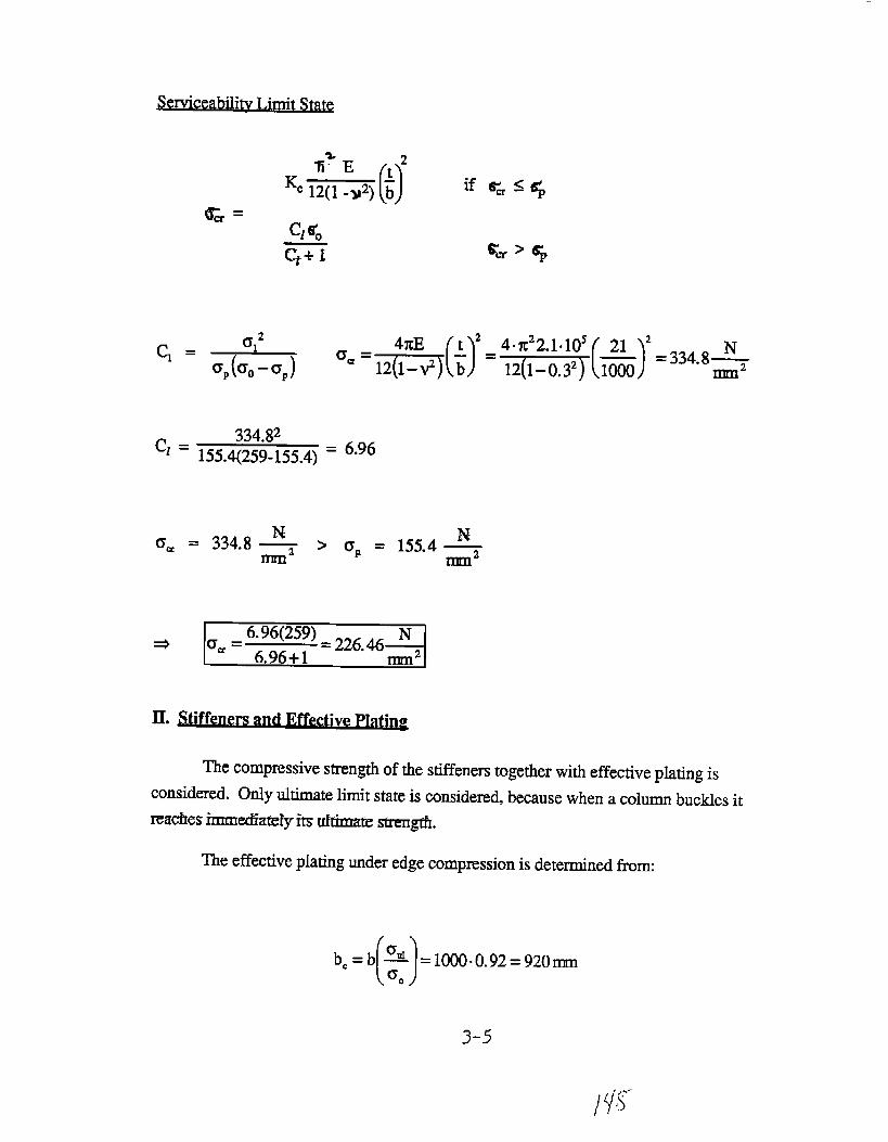
Seficeabll ty Llm t St~. . .
1 i
c1 =a,’
Cp(00- Gp )
334.82Cz = 155.4(259-155.4)
““=&(3’=%%(ia’= 6.96
N=334.8—
mm2
Nam = 334.8 — > up = 155.4 —
mm2 :’
The compressive strength of the stiffeners together with effective plating is
considered. Only ultimate limit state is considered, because when a column buckles it
reaches ilmmediamly its Uhirllm strength.
The effective plating under edge compression is determined from:
()b,=b~ = 1000.0.92= 920mtn60
3-5

..
c=
Ix=
A=
r =
1=
crm=
363.6mm
III– = 142.8A
5400mm
+
Nam = 248 mj3”J2
3-6
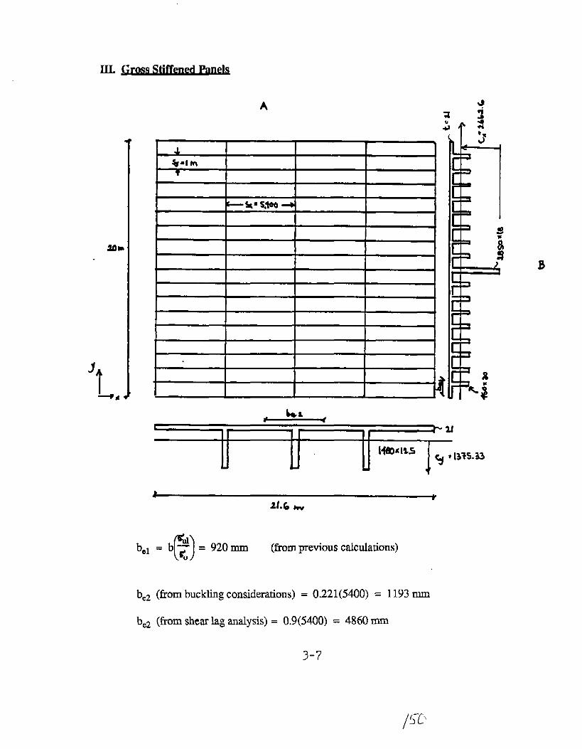
am
A 3“ 2
r)b.1 =b~ =920XIIII (from previous calculations)
bez (horn buckling considerations) = 0.221(5400) = 1193 mm
bez (from shear lag analysis)= 0.9(5400) = 4860 mm
3-7
P-.

ri x~ “mate Limi
A = 3.2816.104 mrr?
IX = 3.2816“ 10SmmA
IY = 1.363“ 109mmA
e = 450.5 distance from neutral exis to shear center yO= 96.9 mm
10 =IX+$+##=
IC = IX+ ~ = 2.035
J = torsional const =
2.34 ‘ 109md
.109-4
E!+@!E=708,(ym,
3 .’
G=L= 2.1 “ 105
2(1 W) 2.6 = 8.077. l~fi
i) Elastic Range: Consider interaction with flexural buckling.
3-8
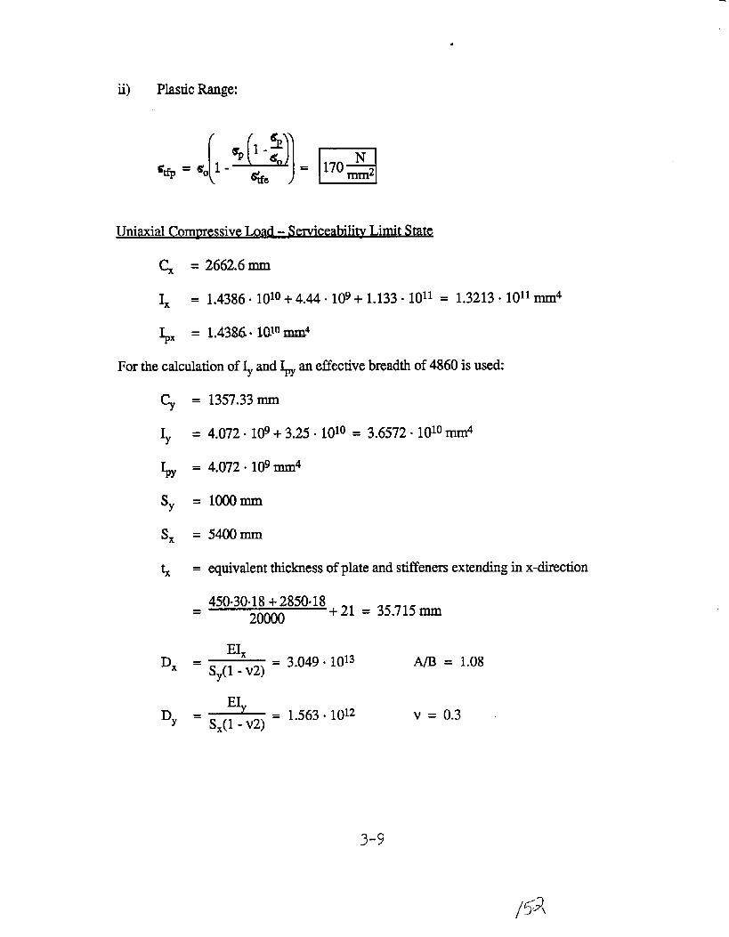
ii) Plastic Range:
Uniaxial Commess ive Lwd - Seticeab ilitv Limit State
G = 2662.6 mm
IX = 1.4386 ‘ 101°+ 4.44 “109+ 1.133“ 1011 = 1.3213.1011 mrr$
% = L43&5“ 1010mzd
For the calculation of $ and ~ an effective breadth of 4860 is used
5 = 1357.33 mm
IY = 4.072“ 109+ 3.25“ 1010 = 3.6572-1010 mm4
b = 4.072“ 109mm4
Sy = looomm
s, = 5400 mm
h = equivalent thickness of plate and stiffeners extending in x-direction
450-30”18 + 2850’18 + 21 = 35 ~15 -=20000
EIXDx =
Sy(l - V2)= 3.049‘ 1013 A/B = 1.08
DY = LSx(l - V2)
= 1.563 “1012 v = 0.3
3-9

3.049”1013“ 1.563”1012 = ~9076 N > ~4“+~
35.715 “200002 -2 P
%=~~&’
El155.4(259 - 155.4) “259 = 259 N190762 -2
155.4(259 - 155.4) + 1
St@ted P.
a (considering only half the panel)
Uniaxial Commess ive Load – Serviceability Limit State
Cx = 363.6
% = 1375.3
IX = 9(6.692) “ 108mm4 = 6.0228 “ 109mm4
3-1o

3.6572 ‘ 1010mm4
IOQOmm
5400 mm
450” 30”9+21 = ~315m.
= 1.39“ 1012
= 1.563“ 1012
4“M 1.3%LHW- 15631(P33.15 “ 100002
L*2L6 WI
From buckling considerations bC = 0.0597”20 = 1193 mm
A = 7.635 “ 1(Ymm2
3-11
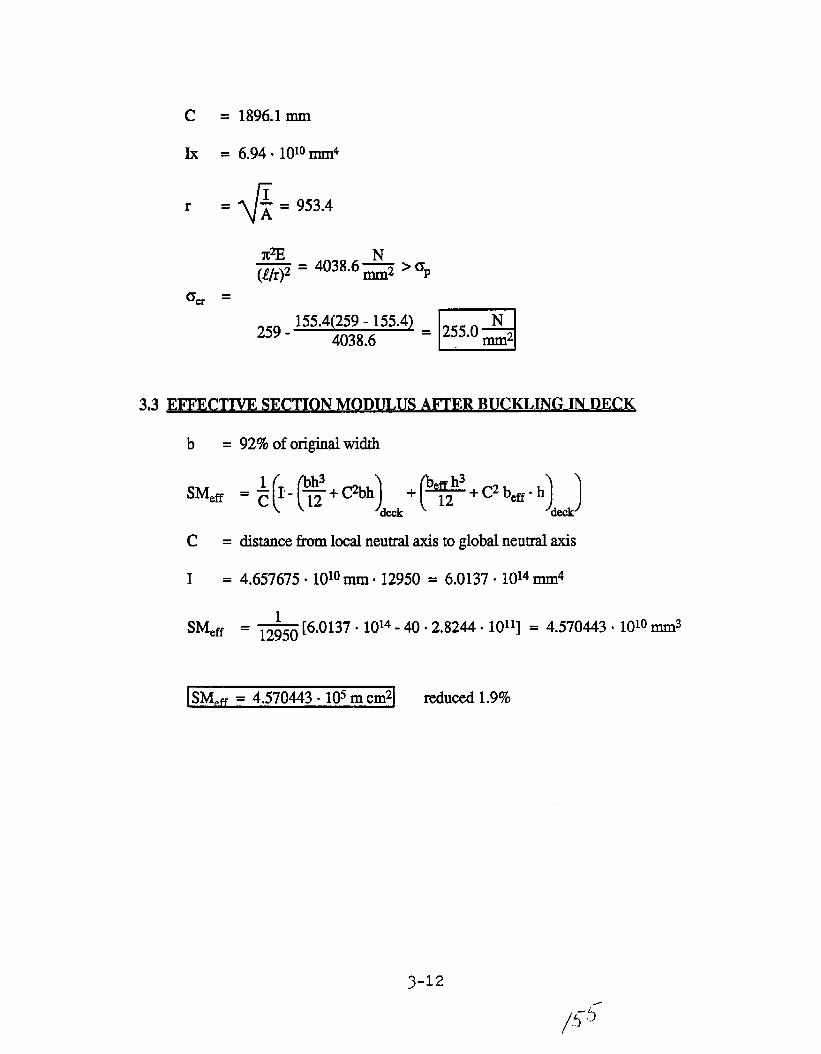
c = 1896.1 mm
Ix = 6.94“ 1010mm4
+
Ir = – = 953.4A
259 155.4(259 -155.44038.6 ‘=Fzl
3.3 EFFECTIVE SECTION MODW AFTER BUC KLING IN DECK
92% of original width
distance from local neutral axis to global neutral axis
4.657675 ‘ 1010mm ‘ 12950 = 6.0137“ 1014nma4
1= ~2950 [6.0137“ 1014-40“ 2.8244. 1011] = 4.570443.1010 n-Im3
~SM,z.W= 4.570443. 1($ m cm21 reduced 1.9?%
3-12
“-.5-/’l
APPENDIX 4
Calculations of Compressive Strength Factor and the Hull Girder Instability
Collapse Moment
4-1

The Compressive Strength Factor for the Critical Panel of the Example Ship(ISSC Fomnula)
%p = (0.960 -t-0.765 kz + 0.176 JP + 0.131 kzfY+ 1.064 Lq)-o.s
p ‘M=w’== 15’3
For the sagging condition, we then have
~ = (-0.172+ 1.548 (pW-0.368 q:) SM . fY
= 0.8 19 SM . fx
4-2

4-3

APPENDIX 5
Calculations of the RMS Values of the Wave Bending Moment for the
Example Ship
5.1 Ultiate Limit State
5.2 Fatigue Limit State
5-1

5.1 RMS OF EXTREME WAVE BENDING MOMENT(ULTIMATE LIMIT STATE)
~ TA
c~ = 0.71
LIB = 6.19 s = H~L = 0U47
B/I’ = 2.62 F, = 0.05 (will use F, = 0.1)
~~
Calculations are made according to seakeeping tables of Ref. 6. From theseakeeping table (see sample interpolation chart on the next page),
rms = 272.7
This vilue is made dimensional by multiplying it with: pg LA
where p =
g =
L=
spetilc density of seawater = 1025 kg/ins
acceleration of gravity = 9.81 rn,kz
length of ship = 260 m.
Dimensional rms = 1.25398.106 kNm
This value may be overestimated a few percent because a Froude number of 0.1 isapplied instead of the value 0.05.
The seakeeping tables are not tabulated for values of F= lower than 0.1.
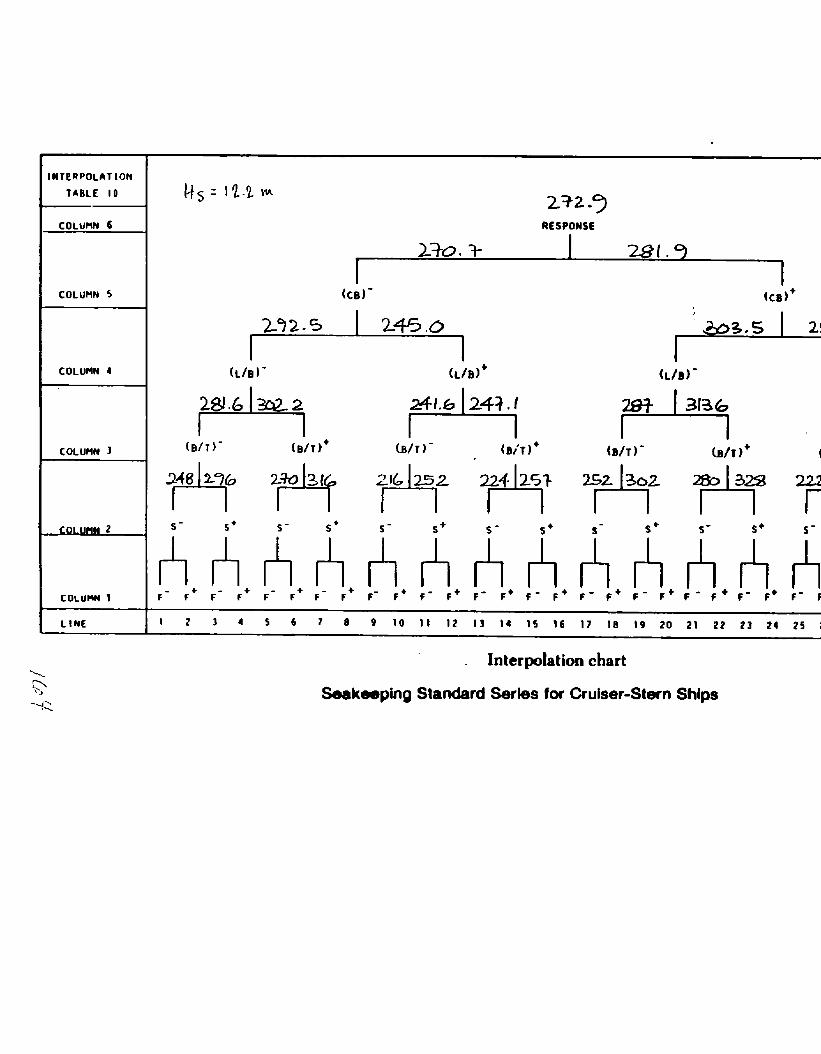
lHWRpOLATIONTABLE 10 !++2.2MA
232.9
COLUMM 6 RESPONSE
230 * ?- 1 Z?(.9I 1
COLUMN5 (CB)- (cEl)+
~ +COLUMN4 (L/B)- (L/B)+ {L/B)-
y&Qq ~1.6,2+7.; ~,q
COLUHH3 {B/T)- (B/T)+ (B/T)- (B7’T)* (B/T)-
pk2f .~ .’”zfi.~ ~=.+
MM2
4 AA AA AA AA AA AA AAAA● + +
COLUPW 1 F- fF-F F-F ‘F- FF-F+ F-F+ F- F+ F- F+ F-F+F ‘F+ F- F+ F- F+ F-F+
..-LiME
II Z3456713 91011 12 13 14 IS 16 17 18 19 20 21 22 23 24 25 2
Interpolation chart--%~
Seak-~ing Standard SerkS for Cruiser-Stern StI~ps-+.
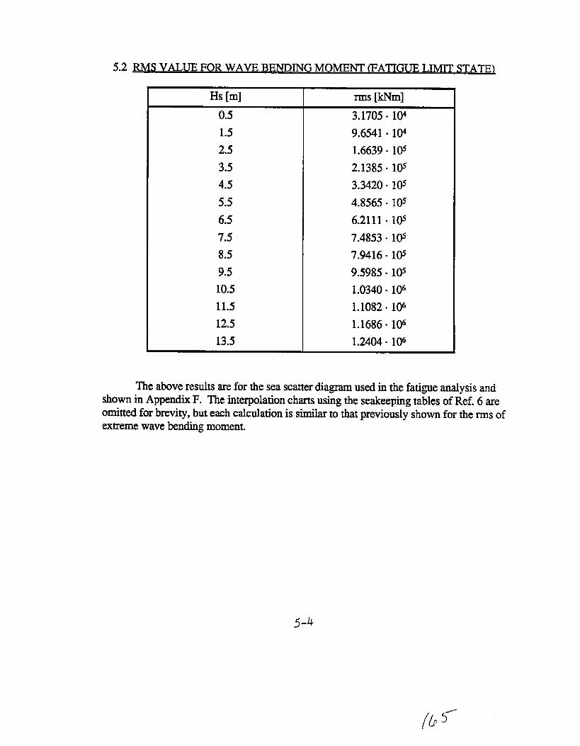
I Hs [m]
0.5
1.5
2.5
3.5
4.5
5.5
6.5
7.5
8.5
9.5
10.5
11.5
12.5
13.5
rms [kNm]
3.1705 “ 1(H
9.6541 “ 1(F
1.6639.105
2.1385 “ 105
3.3420 ‘ 1(F
4.8565 ‘ 105
6.2111 “ 105
7.4853 s 105
7.9416 ‘ 1(P
9.5985. lC$
1.0340 “ 106
1.1082 “ 1(Y
1.1686 “ 1(F
1.2404 “ lW
The above results are for the sea scatter diagram used in the fatigue analysis andshown in Appendix F. The interpolation chats us~g the seakeeping ta;les of Ref. 6 areomitted for brevity, but each calculation is similar to that previously shown for therms ofextreme wave bending moment.
5-4

6-1 / (27
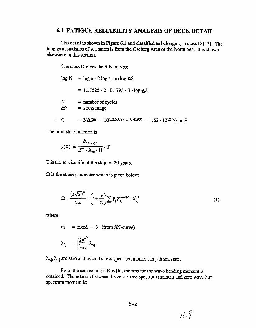
6.1 FATIGUE RELIABILITY ANALYSIS OF DECK DETAIL
The detail is shown in Figure 6.1 and classfled as belonging to class D [13]. Thelong term statistics of sea states is from the Oseberg Area of the North Sea. It is shownelsewhere in this section.
The class D gives the S-N cues:
log N = logs-210gs-mlogAS
= 11.7525 -2.0.1793-3 “log.&S
N = number of cyclesM = stress range
“c.. = ~~m = 10(12.6007-2. 0,4190) = 1,52.1012 N/m2
The limit state function is
T is the setice life of the ship = 20 years.
Clis the stress parameter which is given below:
where
m = freed = 3 (from SN-curve)
kOj,~j are zero and second stress spectrum moment in j-th sea state.
From the seakeeping tables [6], therms for the wave bending moment isobtained. The relation between the zero stress spectrum moment and zero wave b.mspectrum moment is:
(1)
6-2
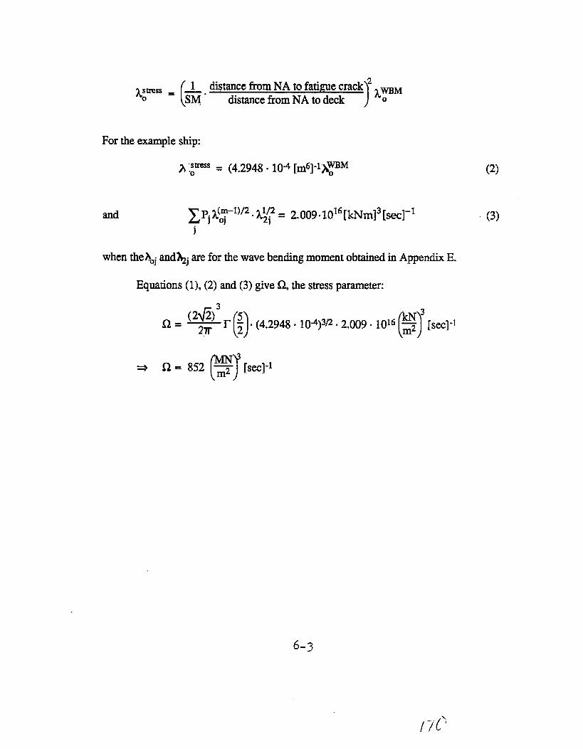
~stress = (1 distance tim NA to fatigue crack 2 ~WMo FQ” distance from NA to deck ) o
For the example ship:
A ~-s = (4.2948. 10~ [md]-lA~M (2)
and XLPj ~~-1)12.i~~ = 2.009 .1016[kNm]3 [see]-l (3)J
when thehoj ~d~j are for the wave bending moment obtained in Appendix E.
(l), (2) and (3) give Q the stress parameter
(2?/Z)3
()
3
2~ ()r ; . (4.2948“ 10$q~ ‘ 2.009.1016 ~ [see]-l
6-3
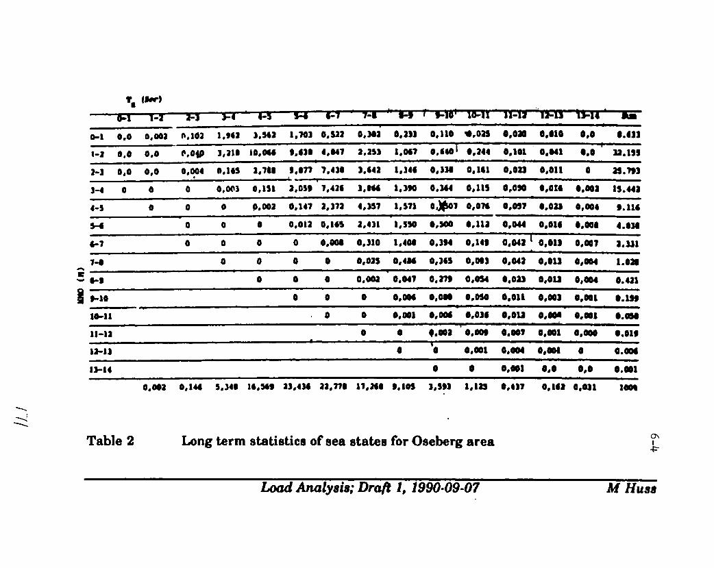
*1 0,0 O.ma 0, ids 1,s41 1,s43 1,701 o,sn 0,3s3 0,133 0,110 *,oa 0,020 0,010 0,0 0.01
1-3 0,0 0,0 COO* 3,319 10,U 9,43n 4.047 a,asl X,00 0,640~ 0,244 0,101 0,041 0,0 22. 19s
2-3 0,0 0,0 ●0,004 II*149 3,740 9,07T 7.430 3,s42 I,34t 0,320 a,141 0,023 0,011 0 a.m
1-4 0 0 0 O,WU o,13i a.099 7,424 3,804 i,m Q,344 0,1s9 0,0* *,OM a,m 19*44a
4-3 9 0 0 p,ml 0,147 2,373 4,357 1,571 o.~T 0,074 0,031 0,022 0,W4 9.118
H o 0 0 O,ota 0,165 2,431 1,s30 0,500 O,lla 0,W4 0,01s O,wo 4.#20
0-1 0 0 0 0 O,ao 0,310 1,400 0,394 0,149 0,041’ O,ou O.m a.ul
n7-o a Q o 0 0,01s 0,400 0,)45 0,00s 0,043 O,ou O,m l.oa
0-s o a o 0,002 0,04? 0,279 0,0s4 0,022 O,ola o*m4 0.421
,-10 00 0 O,mo O,oa 0,0s0 a,on O,m O,m O.M,
f12-1) a o O,ml O,m O,- 0 0.-
12-14 0 0 O,m 0,0 0,0 O**1
2
0,003 0,144 S,340 16,S9 2J,424 32,770 17,240
Table of seaLong term statistics
9,10s 3,393 1,122 0,41? 0,141 O,o)i I*
for Oseberg area m4=
bad Analy8i8; Dra/? 1, 1990-09-07 M HU98

PENDIX7
Typical Input/Output File of CALREL
7.1 User Defined Subroutine for Limit State Function and WaveBending Moment Distribution
7.2 Input Data File
7.3 Output File

CALRel nrx=8 ntp=lDATATITL nlina title1example ship reliability analysis -- deck initial yield, easelFLAG icl,igr10OPTI iop,nil,ni2,tol,opl,op2,0p31,20,4,0.001STAT Igt(i),nge,ngm nv,ids,ex,sg,p3,p4,x01 8
,. ,.I-
sm 1,2,4 .57e5,1.828e4fp 2,2,25.9,1.813Sw 3,1,3.022e6,1.Ow 4,-51,4.855e6,4.3695e5,0.0,0.0,4.855e6Xu 5,1,1.0,0.15XSW 6,1,1.0,0.05Xw 7,1,0.9,0.135Xs 8,1,1.15,0.0345
FORMSEWSORMEXIT
1
i

implicit realdimension %(19= x(5)*x(1)
●8 (a-h,),tp(l)●x(2)-x(
o-z)
6)*x(3)returnend
subroutine udgx(dgx,x,tp,ig)implicit real*8 (a-h,o-z)dimension x(l),dgx(l),tp(l)returnend
subroutine udd(x,par,sg,ids,implicit real*8 (a-h,o-z)dimension x(l),par(4),bnd(2)Pi=3.1415926
-x(7) ●x
(8) ●X
*bnd,
(4)
lb)
factl=(sqrt(6)/pi)*par(l)*par(2)-(0.S772*6/pi**2fact2=dexp(0.5*((pi/sqrt(6))*(par(l)/par(2))-0.5cdf=dexp(-fact2*dexp(-(x(4)●*2)/(2*factl) ))pdf=(x(4)/factl)●fact2*dexp(-(x(4)●*2)/(2*factl)bnd(l)=O.OdOib=lsg=par(2)returnend
)*(par(2)*”2)772))
)‘calf
7-3 /

● ****W********** ● *************** ********************* ● ******
● University of California ●
● Department of Civil Engineering ●
● ●
● CALREL ●
● CAL-Reliability program ●
● Developed by ●
● P.-L. Liu, H.-Z. Lin and A. Der Kiureghian ●
● *● bst Revision: January 1990 ●
● Copyright e 1990 ●
******************● ****************● **********************●*WARNING 2: cormnand not available
>>>> NEW PROB~ <<<<
number of limit-state functions..........ngf= 1number of independent variable groups ...nig= 1total number of random variables ........nrx= 0number of limit-state parameters ........ntp= 1
>>>> INPUT DATA <<<<
example ship reliability analysis -- deck initial yield, easeltype of system .................● ● .● ● **..icl= 1
icl=l . . . . . . . . . . . . . . . . . . . . . . . . . . . . . .* . . . .componenticl=2 ..............................● series systemicl=3 .............................● general system
flag for gradient computation ...........igr= oigr=O ....● ..● ● .● *.*● ● ● ● ● ● ● *..*.● finite differenceigr=l ...................formulasprovided by user
optimization scheme used ................iop=iop=l ......................● .....*.*.HL-RFiop=2 ...● ...................modifid HL-RFiop=3 ..................gradient projectioniop=4 .................sequentialquadratic
msximum number of iteration cycles ......nil=maximum stem in line search ............ni2=
1methodmeth~methodmethod
204
convergence tolerance ................tol= 1.000E-03optimization parameter 1 .............OP1= 1.000E+OOoptimization paremeter 2 .............0P2= 0.000E+OOoptimization parameter 3 .............0P3= 0.000E+OO
statistical data of basic varibles:available probability distributions:deterministic.............ids=Ono-l ...................ids=llognorml ................ids=2gauarla....................ids=3shifted exponential ......ids=4shifted rayleigh .........ids=5uniform ..................ids=6beta .................... .ids=7type i largest value .....ids=lltype i smallest value ....ids=12type ii largest value ....ids=13weibull ..................ids=14user defined .............ids>50
group no.: 1Var ids meansm 2 4.57E+05fp 2 2.59E+01Sw 1 3.02E+06mu 51Xu 1 1.00E+OOXsw 1 1.00E+OOXw 1 9.00E-01
>--Xs 1 1.15E+O0
group type:st. dev. paraml1.83E+04 1.30E+011.81E+O0 3.25E+O01.00E+OO 3.02E+064.37E+05 4.86E+061.50E-01 1.00E+OO5.00E-02 1.00E+OO1.35E-01 9.00E-013.45E-02 1.15E+O0
1param2 pand param44.00E-026.99E-021.00E+OO4.37E+05 0.00E+OO 0.00E+OO1.50E-015.00E-021.35E-013.45E-02 /’7?
7-4
init. pt0.00E+OO0.00E+OO0.00E+OO4.86E+060.00E+OO0.00E+OO0.00E+OO0.00E+OO
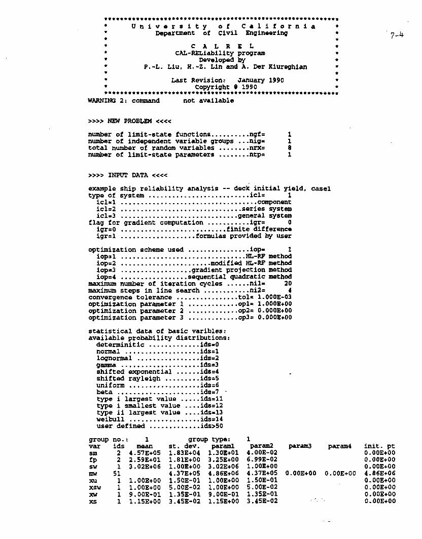
● *T************ ● ***W************ ● ******************* ********● University of California ●
● Department of Civil Engineering ●
● ●
● CA LREL *● CAL-Reliabilityprogram ●
● Developedby ●
* P.-L. Liu, H.-Z. Lin and A. Ikr Kiureghian ●
● ●
● Last Revision: January 1990 ●
● CopyrightQ 1990 ****************w********************************************
WARM% 2: co-d not available
>>>> NEW PROBm <<<<
number of limit-state functions..........ngf= 1number of independentvariable groups ...nig= 1total number of random variables ....*...n.rx= 8number of limit-stateparameters ........ntp= 1
>>>> INPUT DATA <<<<
example ship reliabilityenalysis -- deck initialyield, caaeltype of systan ..........................icl= 1icl=l ............................● ...● ..cumponenticl=2 ...........● ● ...........● ....● .series systemicl=3 . . . . . . . . . . . . ● . . . . . . . . . . . . . . . . .general system
fl;;rf;rgradient computation . . . . . . . . . ..igx= o● . . . . ● . . . . ● ● . . . . ● ● ● . ..**. . .finite difference
igr=l ...................formulasprovidedwuser
. .optimxzatzonscheme used ................iop=iop=l ....● ...........● ● ....● .........ml-miop=2 .......................modifiedHL-RPiop=3 ..................gradientprojectioniop=4 .................sequentialquadratic
nwximum number of iterationcycles ......nil=mximum steps in line search . . . . . . . . . . ..ni2=
1methodmethdmethodmethod
204
convergence tolerance ................tol=1.000E-03optimizationparameter 1 .............opl=1.000E+OOoptimizationparameter 2 .............op2=0.000E+OOoptimizationparameter 3 .....*.......op3= 0.000E+OO
statistical data of basic varibles:
available probability distributions:deterministic. . . . . . . . . . . ..ids=Onormal ...................ids=llognormal ................ids=2gsnmla....................ids=3shifted exponential ......ids=4shifted rayleigh .........ids=5uniform ..................ids=6beta ......................ids=7type i largest value .....ids=lltype i smallest value ....ids=12type ii largest value ....ids=13weibull ..................ids=14user defined .............ids>50
group no.: 1var ids meansm 2 4.57E+05fp 2 2.59E+01Sw 1 3.02E+06m 51m 1 1.00E+OOXsw 1 1.00E+OOw 1 9.00E-01Xs 1 1.15E+O0
group type:st. dev. paraml1.83E+04 1.30E+011.BIE+OO 3.25E+O01.00E+OO 3.02E+064.37E+05 4.86E+061.50E-01 1.00E+OO5.00E-02 1.00E+OO1.35E-01 9.00E-013.45E-02 1.ME+OO
1param2 param34.00E-026.99E-021.00E+OO4.37E+05 0.00E+OO1.50E-015.00E-021.35E-013.45E-02
param4 init. pt0.00E+OO0.00E+OO0.00E+OO
0.00E+OO 4.86E+060.00E+OO0.00E+OO0.00E+OO0.00E+OO
.
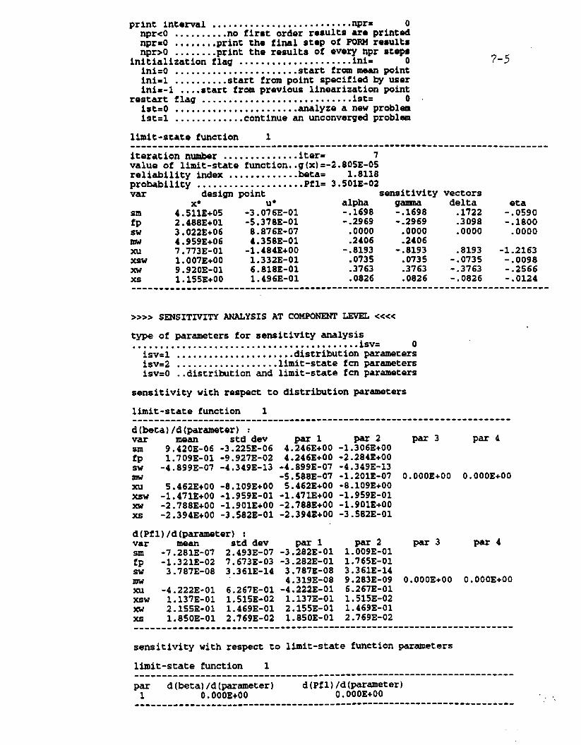
7-5
print inte~al ..*.***.....**.....*...*..npra onprcO ..........no firnt order resultsara printednpr=O ........printthe final stop of PORM rosulksnpr>O ........printthe results of evo~nfpr steps
initializationflag .....● ............... 0ini=o ......................start from me% pointIni=l ..........startfrom point specifiedby userIni=-1 ....startfrom previous linearizationpoint
restart flag ● ...*..*..● .● ● .....*........ist= oist=o .......................analyzeanew problsmist=l .............continuean unconvertedproblan
limit-statefunction 1-----------------------------------------------------------------------------iteration number ..............iter= 7value of limit-statefunction..g(x)=-2.8O5E-O5reliability index ....****● ● ...beta= 1.8118probability ● **..........****...Pfl= 3.501E-02var design point sensitivity
alpha4.5:;E+05 -3.O~;E-01
galunasm -.1698 -.1698fp 2.488E+01 -5.378E-01 -.2969SW 3.022E+06
-.29698.876E-07 .0000 .0000
mw 4.959E+06 4.358E-01 .2406 .2406Xu 7.773E-01 -1.484E+O0 -.8193 -.8193Xsw 1.007E+O0 1.332E-01 .0735 .0735Xw 9.920E-01 6.818E-01 .3763 .3763X2 1.155E+O0 1.496E-01 .0826 .0826---------m------------------------------------------------
vectorsdelta.1722.3098.0000
.8193-.0735-.3763-.0826
eta-.0590-.1800.0000
-1.2163-.0098-.2566-.0124
------- ------- ---.-
>>>> SENSITIVITYANALYSISAT COMPONENTLEVEL <<<<
type of parameters for sensitivityanalysis.● ● .● ● .● .● ● ............● ● ● .*......*● ● **...isv= o
Mm . . . . . . . . . . . . . . . . . . . . ..distributbn p-n=t-isv=2 . . . . . . . . . . . . . . . . . ..limit-state fcn parametersisv=o ..distribution and limit-statefcn parameters
sensitivitywith respect to distributionparameters
limit-statefunction 1----------------------------------------------------------------------d(beca)/d(parameter):Var mean std dev par 1 par2 par 3 par4sm 9.420E-06 -3.225E-06 4.246E+O0-1.306E+O0fp 1.709E-01-9.927E-02 4.246E+O0 -2.284E+O0SW -4.899E-07-4.349E-13-4.899E-07-4.349E-13mw -5.588E-07-1.201E-07 0.000E+OO 0.000E+OOm 5.462E+O0-8.109E+OO 5.462E+O0-8.109E+OOXsW -1.471E+O0-1.959E-01-1.471E+O0-1.959E-01Xw -2.788E+O0-1.901E+O0-2.788E+O0-1.901E+O0Xs -2.394E+O0-3.S82E-01-2.394E+O0-3.S82E-01
d(Pfl)/d(parsmeter):var mean std dev parl par2 par3 par 4sm -7.281E-07 2.493E-07-3.282E-01 1.009E-01fp -1.321E-02 7.673E-03-3.282E-01 1.765E-01Sw 3.787E-08 3.361E-14 3.787E-08 3.361E-14m 4.319E-08 9.283E-09 0.000E+OO 0.000E+OOXu -4.222E-01 6.267E-01-4.222E-01 6.267E-01Xsw 1.137E-01 1.515E-02 1.137E-01 1.515E-02Xw 2.155E-01 1.469E-01 2.155E-01 1.469E-01Xa 1.850E-01 2.769E-02 1.850E-01 2.769E-02----------------------------------------------------------------------
sensitivitywith respect to limit-statefunctionparameters
limit-state function 1-------------------.--------------------------------------------------
y d(beta)/d(~ameter) d(Pfl)/d(par~eter)0.000E+OO 0.000E+OO
--------.........................-------------------------------------

print intomal ● **.*.............*.......npr= onprco ..........no first order results are printednpr=O ........print the final step of POR14resulbsnpr>O ........print the results of every npr steps
initialization flag .....................ini= oIni=o ......................start from mean pointInixl ..........start from point specified by userini=-1 ....start from previous linearization point
restart flag ........● ***................ist= oist=o . . . . . . . . . . . . . . . . . . . . . ..analyze anew problmist=l .............continue an unconverted problem
7“5
limit-state function 1..--.-.-.................-------------------------------......----------..a--iteration number ..............iter= 7value of limit-state function..g(x)=-2.8O5E-O5reliability index .............beta= 1.8118probability ....................Pfl=3 .501E-02var design point sensitivity vectors
x* alpha delta-3.O%E-01
gamllasm
eta4.511E+05 -.1698 -.1698 .1722 -.0590
fp 2.488E+01 -5.378E-01 -.2969 -.2969 .3098Sw 3.022E+06 8.876E-07 .0000
-.1800.0000 .0000
mw 4.959E+06.0000
4.358E-01 .2406 .2406m 7.773E-01 -1.484E+O0 -.8193 -.8193 .8193 -1.2163Xsw 1.007E+O0 1.332E-01 .0735 .0735 -.0735 -.0098Xw 9.920E-01 6.818E-01 .3763 .3763 -.3763 -.2566Xs 1.155E+O0 1.496E-01 .0826 .0826 -.0826 -.0124------------.---c-.-a---~c-ss--a--------.-------~.------------S.a---------ti--
>>>> SENSIT~ITY ANALYSIS AT COMPONENT LEVEL <<<<
type of parameters for sensitivity analysis..● .● .........,...,● ..,.,.,..,...● ...● ....isv=isv=l
o......................distributionparameters
isv=2 ...................limit-state fcn parametersisv=o ..distributionand limit-state fcn parameters
sensitivity with respect to distribution parameters
limit-state function 1.-------.-a-----=--------------------------------.-------------.------d(beta)/d(parameter) :var std dev par 1 par2
9.%%-06 -3.22SE-06 4.246E+O0 -1.306E+O0par 3 par 4
smfp 1.709E-01 -9.927E-02 4.246E+O0 -2.284E+O0Sw -4.899E-07 -4.349E-13 -4.899E-07 -4.349E-13mw -5.588E-07 -1.201E-07 0.000E+OO 0.000E+OOXu 5.462E+O0 -8.109E+OO 5.462E+O0 -8.109E+OOXsw -1.471E+O0 -1.959E-01 -1.471E+O0 -1.959E-01m -2.788E+O0 -1.901E+O0 -2.788E+O0 -1.901E+O0Xs -2.394E+O0 -3.582E-01 -2.394E+O0 -3.582E-01
d(Pfl)/d(parsmeter) :var mean std dev par 1 par 2 par3 par 4sm -7.281E-07 2.493W07 -3.282E-01 1.009E-01fp -1.321E-02 7.673E-03 -3.282E-01 1.76SE-01Sw 3.787E-08 3.361E-14 3.787E-08 3.361E-14mw 4.319E-08 9.283E-09 0.000E~OO 0.000E+OOXu -4.222E-01 6.267E-01 -4.222E-01 6.267E-01Xsw 1.137E-01 1.515E-02 1.137E-01 1.515E-02Xw 2.155E-01 1.469E-01 2.155E-01 1.469E-01X2 1.850E-01 2.769E-02 1.850E-01 2.769E-02------ ------ ------ ------ ------ ------ ------ ------ --- -- ----
sensitivity with respect to limit-state function parameters
limit-state function 1------------------==.------------a---------+-----------py d(beta)/d(paratneter) d(Pfl)/d(parameter)
0.000E+OO 0.000E+OO-------------.---.------------------------------..-------- -----
,~;”:.v;::::,,!,,$,~,d’’’:,(]
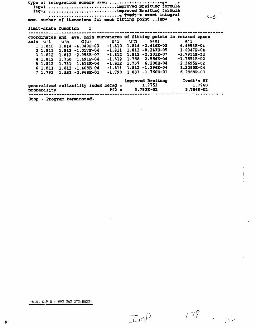
type 01 Lntegracion scneme uses . . . . . .. ** ***. .**m. .&~W-itg=l ......*....*........● ...● ..iwrOVOd BreiLung fonnul;itg=2 . . . . . . . . . . . . . . ..* . ● ● . . ● . ..* improved Braitung formula
. . . . . . . . ● . . . . . . . . ● ● w. ● ** ● ● *● & medc”s met integralmax. number of iterations for each fitting point ..hp= 4 7-6
limit-state function 1........---------------------------------------------------------------------coordinates and ave. main cunatures of fitting points in rotated spaceaxis U“i u-n G(u) U’i u’n G(u) a’i
1 1.810 1.S14 -4.040E-03 -1.810 1.814 -2.416E-03 6.4993E-042 1.811 1.812 -1.017E-04 -1.811 1.812 -8.243E-05 1.0947E-043 1.812 1.812 -2.953E-07 -1.812 1.812 -2.201E-07 -3.7914E-124 1.812 1.750 1.491E-04 -1.812 1.758 2.554E-04 -1.7551E-025 1.812 1.731 1.514E-04 -1.812 1.737 6.208E-04 -2.3695E-026 1.811 1.812 -1.408E-04 -1.811 1.812 -1.296E-04 1.3290E-047 1.792 1.831 -2.968E-01 -1.790 1.833 -1.760E-01 6.2968E-03
improv~ Br::tung Wedt’s EIgeneralized reliability index betag = 1.7760probability Pf2 = 3.79;E-02 3.786E-02..........----..........-----------------------------------------------------stop - Program terminated.
*U.S. E.P.O. :1993-343-273:80231
SHIP STRUCTURE COMMITTEE PUBLICATIONS
SSC-351 ~;9#troduction to Structural Reliability Theory by Alaa E. Mansour
SSC-352 Marine Structural Steel Touqhness Data Bank by J. G. Kaufman andM. Prager 1990
SSC-353 fmaysis of Wave Characteristics in Extreme Seas by William H. Buckley
SSC-354 Structural Redundancy for Discrete and Continuous Systems by P. K.Das and J. F. Garside 1990
SSC-355 Relation of Inspection Findincis to Fatiaue Reliability by M. Shinozuka1989
SSC-356 Fatiaue Performance Under Multiaxial Loai by Karl A. Stambaugh,Paul R. Van Mater, Jr., and William H. Munse 1990
SSC-357 Carbon Equivalence and Weldabilitv of Microalloved Steels by C. D.Lundin, T. P. S. Gill, C. Y. P. Qiao, Y. Wang, and K. K. Kang 1990
SSC-358 Structural Behavior After Fatiaue by Brian N. Leis 1987
SSC-359 Hydrodynamic Hull Dampinq (Phase 1)by V. Ankudinov 1987
SSC-360 Use of Fiber Reinforced Plastic in Marine Structures by Eric Greene1990
SSC-361
SSC-362
SSC-363
ssC-364
SSC-365
SSC-366
SSC-367
None
Hull Strappinq of Ships by Nedret S. Basar and Roderick B. Hulls 1990
Shipboard Wave Heiaht sensor by R. Atwater 1990
Uncertainties in Stress Analvsis on Marine Structures by E. Nikolaidisand P. Kaplan 1991
Inelastic Deformation of Plate Panels by Eric Jennings, Kim Grubbs,Charles Zanis, and Louis Raymond 1991
Marine Structural Intearitv Prowams (MSIP) by Robert G. Bea 1992
Threshold Corrosion Fatique of Welded Shipbuilding Steels by G. H.Reynolds and J. A. Todd 1992
Fatiaue Technoloav Assessment and Strategies for Fatique Avoidance inMarine Structures by C. C. Capanaglu
Ship Structure Committee Publications - A Special Bibliography
r
L.

COMM1l’TEE ON MARINE STRUCTURES
Commission on Engineering and Technical Systems
National Academy of Sciences - National Research C~uncil
The COMMl~EE ON MARINE STRUCTURES has technical cognizance over the
interagency Ship Structure Committee’s research program.
Peter M. Palermo Chairman, Alexandria, VA
Mark Y. Berman, Amoco Production Company, Tulsa, OK
Subrata K. Chakrabarti, Chicago Bridge and Iron, Plainfield, IL
Rolf D. Glasfeld, General Dynamics Corporation, Groton, GT
William H. Hartt, Florida Atlantic University, Boca Raton, FL
Robert Sielski, National Research Council, Washington, DC
Robert G. Loewy, NAE, Rensselaer Polytechnic Institute, Troy, NY
Stephen E. Sharpe, Ship Structure Committee, Washington, DC
LOADS WORK GROUP
Subrata K. Chakrabarti Chairman, Chicago Bridge and Iron Company, Plainfield, IL
Howard M. Bunch, University of Michigan, Ann Arbor, Ml
Peter A. Gale, John J. McMu[len Associates, Arlington, VA
Hsien Yun Jan, Martech Incorporated, Neshanic Station, NJ
Naresh Maniar, M. Rosenblatt & Son, Incorporated, New York, NY
Solomon C. S. Yim, Oregon State University, Corvallis, OR
MATERIALS WORK GROUP
William H. Hartt Chairman, Florida Atlantic University, Boca Raton, FL
Santiago lbarra, Jr., Amoco Corporation, Naperville, IL
John Land~~, University of Tennessee, Knoxvillq TN
Barbara A. Shaw, Pennsylvania State University, University Park, PA
James M. Sawhill, Jr., Newport News Shipbuilding, Newport News, VA
Bruce R. Somers, Lehigh University, Bethlehem, PA
Jerry G. Williams, Conoco, Inc., Ponca City, OK
c“3 @J!3/ 4’5$