5. Properties of Graphs

ConnectedComponents

? ConnectedComponents

ConnectedComponents@gD gives the verticesof graph g partitioned into connected components.

ConnectedComponents@s = RegularGraph@1, 10DD881, 3<, 82, 7<, 84, 5<, 86, 10<, 88, 9<<

ShowGraph@s, VertexNumber -> OnD

1

23

4

5

6

7 8

9

10

� Graphics �

c = ConnectedComponents@s = RegularGraph@2, 20DD881, 6, 15, 5, 20, 18, 16, 10<, 82, 3, 12, 17, 4, 19<, 87, 8, 9, 14, 11, 13<<

2 Chapter5.nb

ShowGraph@s, VertexNumber -> On,VertexNumberColor -> Purple, Background -> YellowD

1

2

3

45

6

7

8

9

10

11

12

13

1415

16

17

18

19

20

� Graphics �

Chapter5.nb 3

ShowGraph@InduceSubgraph@s, c@@1DDDD

� Graphics �

a = GraphUnion@Wheel@5D, Star@10DD;ConnectedComponents@ a D881, 2, 3, 4, 5<, 86, 15, 7, 8, 9, 10, 11, 12, 13, 14<<a = GraphUnion @10, Star@10DD; ConnectedComponents@ a D881, 10, 2, 3, 4, 5, 6, 7, 8, 9<, 811, 20, 12, 13, 14, 15, 16, 17, 18, 19<,821, 30, 22, 23, 24, 25, 26, 27, 28, 29<, 831, 40, 32, 33, 34, 35, 36, 37, 38, 39<,841, 50, 42, 43, 44, 45, 46, 47, 48, 49<, 851, 60, 52, 53, 54, 55, 56, 57, 58, 59<,861, 70, 62, 63, 64, 65, 66, 67, 68, 69<, 871, 80, 72, 73, 74, 75, 76, 77, 78, 79<,881, 90, 82, 83, 84, 85, 86, 87, 88, 89<, 891, 100, 92, 93, 94, 95, 96, 97, 98, 99<<

TIMING DISCUSSION

First we have a comparison between the new and old implementations of ConnectedComponents. As can be seen from the tables of timings given below, the new implementation is dramatically faster than the old implementation − factor of speed ranges from 80 to more than 100.

4 Chapter5.nb

$RecursionLimit = 100000;

g = Table@DiscreteMath‘OldCombinatorica‘RandomGraph@i * 100, 0.01D, 8i, 5<D;h = Table@RandomGraph@i * 100, 0.01D, 8i, 10<D8�Graph:<52, 100, Undirected>�, �Graph:<194, 200, Undirected>�,

�Graph:<433, 300, Undirected>�, �Graph:<812, 400, Undirected>�,�Graph:<1264, 500, Undirected>�, �Graph:<1804, 600, Undirected>�,�Graph:<2386, 700, Undirected>�, �Graph:<3313, 800, Undirected>�,�Graph:<4034, 900, Undirected>�, �Graph:<4922, 1000, Undirected>�<Table@8Length@DiscreteMath‘OldCombinatorica‘ConnectedComponents@g@@iDDDD,Length@ConnectedComponents@h@@iDDDD<, 8i, 5<D

8851, 49<, 842, 26<, 815, 13<, 812, 8<, 83, 3<<ort = Table@Timing@DiscreteMath‘OldCombinatorica‘ConnectedComponents@g@@iDDD;D, 8i, 5<D

882.407 Second, Null<, 87.593 Second, Null<,86.282 Second, Null<, 88.75 Second, Null<, 83.562 Second, Null<<rt = Table@ Timing@ ConnectedComponents@ h@@iDD D; D, 8i, 10<D880.016 Second, Null<, 80.031 Second, Null<,80.047 Second, Null<, 80.094 Second, Null<,80.14 Second, Null<, 80.188 Second, Null<, 80.25 Second, Null<,80.343 Second, Null<, 80.422 Second, Null<, 80.516 Second, Null<<

The running time plot for ConnectedComponents confirms that the running time grows quadratically in the size of the graph. However, the experiment might be misleading since the expected number of edges in the random graph also grows quadratically. So I do a second experiment below. In that experiment the running time seems almost linear! Note that in this experiment, the number of vertices and the number of edges are growing in a roughly linear fashion.

Chapter5.nb 5

p1 = ListPlot@ Map@ #@@1, 1DD &, rtD, PlotJoined -> TrueD

4 6 8 10

0.1

0.2

0.3

0.4

0.5

� Graphics �

gt = Table@ InduceSubgraph@GridGraph@20, 10 * iD,RandomKSubset@ Range@ 200 * iD, 100 * iDD, 8i, 10<D;

Map@ V, gtD8100, 200, 300, 400, 500, 600, 700, 800, 900, 1000<Map@M, gtD892, 210, 287, 369, 475, 588, 700, 791, 895, 974<rt = Table@ Timing@ ConnectedComponents@ gt@@iDD D;D, 8i, 10<D880. Second, Null<, 80.031 Second, Null<,80.047 Second, Null<, 80.047 Second, Null<,80.078 Second, Null<, 80.078 Second, Null<, 80.11 Second, Null<,80.125 Second, Null<, 80.156 Second, Null<, 80.156 Second, Null<<Clear@gtD

6 Chapter5.nb

ListPlot@ Map@ #@@1, 1DD &, rtD, PlotJoined -> TrueD

4 6 8 10

0.025

0.05

0.075

0.1

0.125

0.15

� Graphics �

The following experiment shows that BFS may be faster than DFS and it might be better to use BFS in the new Connected-Components. However, I will wait to make this change to ConnectedComponents because I expect both DFS and BFS to be speeded up.

s = GridGraph@50, 50D;8Timing@DepthFirstTraversal@s, 1D;D, Timing@BreadthFirstTraversal@s, 1 D;D<882.547 Second, Null<, 81.235 Second, Null<<

Here is a larger experiment with ConnectedComponents.

s = InduceSubgraph@GridGraph@70, 70D, RandomSubset@Range@4900DDD�Graph:<2424, 2459, Undirected>�

V@sD2459

M@sD2424

Chapter5.nb 7

ShowGraph@s, VertexStyle -> Disc@0DD

� Graphics �

Timing@c = ConnectedComponents@sD;D80.562 Second, Null<Length@cD343

Max@Map@Length, cDD143

Only 11 seconds for a graph with 5030 vertices and lots of components!

8 Chapter5.nb

g = GridGraph@100, 100D�Graph:<19800, 10000, Undirected>�

h = InduceSubgraph@g, RandomSubset@Range@10000DDD;ShowGraph@h, VertexStyle -> Disc@0DD

� Graphics �

V@hD4940

Chapter5.nb 9

M@hD4827

Timing@c = ConnectedComponents@hD;D81.531 Second, Null<8Length@cD, Max@Map@Length, cDD<8729, 177<

ConnectedQ

? ConnectedQ

ConnectedQ@gD yields True if undirected graph g is connected. If g isdirected, the function returns True if the underlying undirected graphis connected. ConnectedQ@g, StrongD and ConnectedQ@g, WeakD yield Trueif the directed graph g is strongly or weakly connected, respectively.

ConnectedQ@Wheel@10DDTrue

ConnectedQ@DeleteVertices@Star@10D, 810<DDFalse

ConnectedQ@Wheel@10D, WeakDConnectedQ@�Graph:<18, 10, Undirected>�, WeakD

10 Chapter5.nb

ConnectedQ@OrientGraph@Wheel@10DD, StrongDTrue

ConnectedQ@SetGraphOptions@RandomTree@20D, EdgeDirection ® OnD, StrongDFalse

ConnectedQ@SetGraphOptions@RandomTree@20D, EdgeDirection ® OnD, WeakDTrue

NOTES

* ConnectedQ with the strong and weak options works only on directed graphs.

ConnectedQ@ Wheel@10D, WeakDConnectedQ@�Graph:<18, 10, Undirected>�, WeakDConnectedQ@ Wheel@10D, StrongDConnectedQ@�Graph:<18, 10, Undirected>�, StrongDg = SetGraphOptions@ Wheel@10D, EdgeDirection -> OnD;

Chapter5.nb 11

ShowGraph@ g , VertexNumber -> Text@ 80.03, 0<,TextStyle -> 8FontSize -> 14, FontColor -> Blue, FontWeight -> Bold<D,

PlotRange -> Large@0.05DD

1

23

4

5

67

8

910

� Graphics �

ConnectedQ@ g, WeakDTrue

ConnectedQ@g, StrongDFalse

h = AddEdges@g, 8889, 1<<, 8810, 1<<<D;ConnectedQ@h, StrongDTrue

12 Chapter5.nb

ConnectedQ@h, WeakDTrue

ShowGraph@ h D

� Graphics �

WeaklyConnectedComponents, StronglyConnectedComponents

? WeaklyConnectedComponents

WeaklyConnectedComponents@gD gives the weakly connectedcomponents of directed graph g as lists of vertices.

? StronglyConnectedComponents

StronglyConnectedComponents@gD gives the stronglyconnected components of directed graph g as lists of vertices.

s = SetGraphOptions@GridGraph@5, 6D, EdgeDirection -> OnD;

Chapter5.nb 13

ShowGraph@s, VertexNumber -> Text@8-0.04, -0.04<D, PlotRange -> Large@0.05DD

1 2 3 4 5

6 7 8 9 10

11 12 13 14 15

16 17 18 19 20

21 22 23 24 25

26 27 28 29 30

� Graphics �

WeaklyConnectedComponents@sD881, 2, 3, 4, 5, 10, 9, 8, 7, 6, 11, 12, 13, 14, 15,20, 19, 18, 17, 16, 21, 22, 23, 24, 25, 30, 29, 28, 27, 26<<

StronglyConnectedComponents@sD8830<, 825<, 820<, 815<, 810<, 85<, 829<, 824<,819<, 814<, 89<, 84<, 828<, 823<, 818<, 813<, 88<, 83<, 827<,822<, 817<, 812<, 87<, 82<, 826<, 821<, 816<, 811<, 86<, 81<<s = AddEdges@s, 88830, 1<<<D;

14 Chapter5.nb

StronglyConnectedComponents@ s D8826, 21, 16, 11, 6, 27, 22, 17, 12, 7, 28, 23, 18,13, 8, 29, 24, 19, 14, 9, 30, 25, 20, 15, 10, 5, 4, 3, 2, 1<<

NOTES

* The above example shows that s is almost strongly connected − addition of one edge makes it strongly connected.

TIMING DISCUSSION

WeaklyConnectedComponents simply turns the graph into an undirected graph and runs the function ConnectedCompo-nents on that. Therefore its running time is completely dominated by the running time of ConnectedComponents.

Here I focus on the running time of StronglyConnectedComponents. As the plot below shows StronglyConnectedCompo-nents has running time that is roughly quadratic in the size of the graph. This should not be the case and I should try to recode StronglyConnectedComponents so that it runs in linear time.

TO DO

* Redo strongly connected components so that it runs in linear time.

The timings and plots further below make it clear that the new implementation of StronglyConnectedComponents[...] is much faster than the old implementation. The plots seem to indicate that both functions take quadratic time with different constants.

gt = Table@ RandomGraph@100 i, N@1 � 100 iD, DirectedD, 8i, 10<D;rt = Table@ Timing@StronglyConnectedComponents@gt@@iDDD;D, 8i, 10<D880.031 Second, Null<, 80.078 Second, Null<,80.203 Second, Null<, 80.453 Second, Null<,80.906 Second, Null<, 81.641 Second, Null<, 82.734 Second, Null<,84.329 Second, Null<, 86.609 Second, Null<, 89.375 Second, Null<<Map@V, gtD8100, 200, 300, 400, 500, 600, 700, 800, 900, 1000<Map@M, gtD8105, 774, 2681, 6422, 12569, 21526, 33894, 51405, 72820, 99907<

Chapter5.nb 15

ListPlot@ Map@ #@@1, 1DD &, rtD, PlotJoined -> TrueD

4 6 8 10

2

4

6

8

� Graphics �

ogt = Table@DiscreteMath‘OldCombinatorica‘RandomGraph@100 i, N@1 � 100 iD, 80, 1<D, 8i, 5<D;

ort =Table@ Timing@ DiscreteMath‘OldCombinatorica‘StronglyConnectedComponents@

ogt@@iDD D;D, 8i, 5<D880.094 Second, Null<, 80.219 Second, Null<,80.531 Second, Null<, 80.984 Second, Null<, 81.641 Second, Null<<Clear@MultipleListPlotD; Remove@ MultipleListPlotD;<< Graphics‘MultipleListPlot‘

16 Chapter5.nb

MultipleListPlot@Map@#@@1, 1DD &, rtD,Map@ #@@1, 1DD &, ortD, PlotJoined -> TrueD

2 4 6 8 10

1

2

3

4

5

6

� Graphics �

g = SetGraphOptions@GridGraph@70, 70D, EdgeDirection -> OnD;8Timing@cw = WeaklyConnectedComponents@gD;D,Timing@cs = StronglyConnectedComponents@gD;D, Length@cwD, Length@csD<

8812.156 Second, Null<, 85.5 Second, Null<, 1, 4900<OrientGraph

? OrientGraph

OrientGraph@gD assigns a direction to each edge of a bridgeless,undirected graph g, so that the graph is strongly connected.

g = GridGraph@10, 10D;

Chapter5.nb 17

ShowGraph@ h = OrientGraph@ GridGraph@10, 10D D D

� Graphics �

Length@StronglyConnectedComponents@hDD1

g = RandomGraph@20, .6D;Bridges@gD8<

18 Chapter5.nb

Length@ StronglyConnectedComponents@SetGraphOptions@g, EdgeDirection -> OnDD D20

h = OrientGraph@gD;Length@ StronglyConnectedComponents@gD D1

TIMING DISCUSSION

OrientGraph in new Combinatorica is extremely slow!! About 227 seconds for 400 vertex grid graph! Most of the time is however taken by ExtractCycles. So ExtractCycles is in need of major repair. One immediate improvement is for ExtractCy-cles to not compute the new adjacency list representation from scratch after each cycle has been deleted. Of course, OrientGraph in "old" Combinatorica seems 4 times slower (based on one sample point).

I wonder if it is possible to do this in linear time. Even if it isn’t, I am sure it is possible to do this in much more speedy fashion.

TO DO

Speed up ExtractCycles[...]

g = GridGraph@20, 20D;Timing @ OrientGraph@gD;D849.906 Second, Null<Timing@ ExtractCycles@gD; D848.813 Second, Null<h = DiscreteMath‘OldCombinatorica‘GridGraph@20, 20D;Timing@ DiscreteMath‘OldCombinatorica‘OrientGraph@hD; D8181.047 Second, Null<

BiconnectedComponents

Chapter5.nb 19

? BiconnectedComponents

BiconnectedComponents@gD gives a list of the biconnected components ofgraph g. If g is directed, the underlying undirected graph is used.

BiconnectedComponents@RandomTree@100DD881, 5<, 828, 84<, 86, 51<, 82, 19<, 814, 19<, 814, 51<, 885, 99<, 848, 85<,848, 75<, 813, 76<, 815, 76<, 815, 63<, 863, 75<, 845, 75<, 88, 45<, 88, 24<,823, 24<, 823, 51<, 851, 89<, 818, 59<, 830, 43<, 838, 43<, 886, 90<, 833, 86<,827, 33<, 827, 41<, 827, 57<, 838, 57<, 838, 67<, 838, 78<, 812, 87<,812, 98<, 87, 98<, 87, 74<, 835, 65<, 816, 65<, 816, 74<, 821, 39<, 826, 53<,849, 64<, 826, 64<, 826, 83<, 855, 60<, 83, 50<, 831, 40<, 840, 50<, 850, 70<,873, 100<, 850, 100<, 850, 80<, 820, 80<, 820, 56<, 856, 93<, 861, 93<,855, 93<, 855, 83<, 839, 83<, 839, 74<, 822, 74<, 822, 77<, 811, 91<, 834, 69<,844, 47<, 847, 69<, 852, 66<, 832, 58<, 836, 82<, 858, 82<, 854, 58<,854, 66<, 866, 69<, 888, 96<, 869, 88<, 817, 69<, 817, 72<, 872, 91<,877, 91<, 877, 78<, 859, 78<, 859, 89<, 89, 46<, 89, 68<, 89, 25<, 837, 81<,837, 71<, 825, 71<, 825, 42<, 842, 79<, 810, 95<, 810, 97<, 810, 92<,879, 92<, 829, 79<, 829, 62<, 862, 89<, 884, 89<, 81, 84<, 84, 94<, 81, 94<<Length@%D99

BiconnectedComponents@Cycle@100DD881, 2, 3, 4, 5, 6, 7, 8, 9, 10, 11, 12, 13, 14, 15, 16, 17, 18, 19, 20, 21, 22, 23,24, 25, 26, 27, 28, 29, 30, 31, 32, 33, 34, 35, 36, 37, 38, 39, 40, 41, 42, 43,44, 45, 46, 47, 48, 49, 50, 51, 52, 53, 54, 55, 56, 57, 58, 59, 60, 61, 62,63, 64, 65, 66, 67, 68, 69, 70, 71, 72, 73, 74, 75, 76, 77, 78, 79, 80, 81,82, 83, 84, 85, 86, 87, 88, 89, 90, 91, 92, 93, 94, 95, 96, 97, 98, 99, 100<<

20 Chapter5.nb

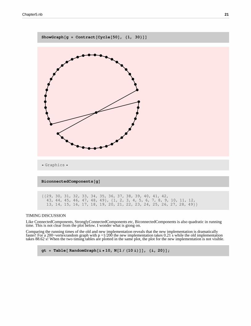
ShowGraph@g = Contract@Cycle@50D, 81, 30<DD

� Graphics �

BiconnectedComponents@gD8829, 30, 31, 32, 33, 34, 35, 36, 37, 38, 39, 40, 41, 42,43, 44, 45, 46, 47, 48, 49<, 81, 2, 3, 4, 5, 6, 7, 8, 9, 10, 11, 12,13, 14, 15, 16, 17, 18, 19, 20, 21, 22, 23, 24, 25, 26, 27, 28, 49<<

TIMING DISCUSSION

Like ConnectedComponents, StronglyConnectedComponents etc, BiconnectedComponents is also quadratic in running time. This is not clear from the plot below. I wonder what is giong on.

Comparing the running times of the old and new implementation reveals that the new implementation is dramatically faster! For a 200−vertex random graph with p =1/200 the new implementation takes 0.21 s while the old implementation takes 88.62 s! When the two timing tables are plotted in the same plot, the plot for the new implementation is not visible.

gt = Table@ RandomGraph@i * 10, N@1 � H10 iLDD, 8i, 20<D;

Chapter5.nb 21

rt = Table@Timing@ BiconnectedComponents@ gt@@iDD D;D, 8i, 20<D880. Second, Null<, 80.015 Second, Null<,80. Second, Null<, 80.016 Second, Null<, 80.016 Second, Null<,80.015 Second, Null<, 80.016 Second, Null<, 80.031 Second, Null<,80.031 Second, Null<, 80.032 Second, Null<, 80.031 Second, Null<,80.031 Second, Null<, 80.047 Second, Null<, 80.047 Second, Null<,80.047 Second, Null<, 80.047 Second, Null<, 80.062 Second, Null<,80.047 Second, Null<, 80.062 Second, Null<, 80.063 Second, Null<<ListPlot@ Map@ #@@1, 1DD &, rtD, PlotJoined -> TrueD

5 10 15 20

0.01

0.02

0.03

0.04

0.05

0.06

� Graphics �

gt =Table@ DiscreteMath‘OldCombinatorica‘RandomGraph@i * 10, 1 � H10 iLD, 8i, 20<D;

ort = Table@Timing@DiscreteMath‘OldCombinatorica‘BiconnectedComponents@ gt@@iDD D;D, 8i, 20<D

880.016 Second, Null<, 80.031 Second, Null<,80.109 Second, Null<, 80.203 Second, Null<, 80.313 Second, Null<,80.578 Second, Null<, 81.031 Second, Null<, 81.078 Second, Null<,81.844 Second, Null<, 82.469 Second, Null<, 83.031 Second, Null<,84.141 Second, Null<, 85.14 Second, Null<, 86.829 Second, Null<,89.546 Second, Null<, 810.969 Second, Null<, 811.172 Second, Null<,813.172 Second, Null<, 816.484 Second, Null<, 822. Second, Null<<

22 Chapter5.nb

MultipleListPlot@ Map@ #@@1, 1DD &, rtD,Map@ #@@1, 1DD &, ortD, PlotJoined -> True D

5 10 15 20

5

10

15

20

� Graphics �

TO DO

* Also we should definitely produce the Block−Cutpoint−Tree of a graph. It would be a nice illustration of the excellent properties that blocks and cutpoints have.

* Here we might also consider discussing the connectivity approximation algorithms of Khuller. These are easily imple-mented and so it might not be a bad idea to include a few of these.

BiconnectedQ

? BiconnectedQ

BiconnectedQ@gD yields True if graph g is biconnected.If g is directed, the underlying undirected graph is used.

g = GridGraph@4, 4D;BiconnectedQ@gDTrue

BiconnectedQ@CompleteGraph@10DDTrue

Chapter5.nb 23

BiconnectedQ@GraphUnion@CompleteGraph@10D, CompleteGraph@10DDDFalse

BiconnectedQ@g = Contract@GraphUnion@CompleteGraph@10D, CompleteGraph@10DD, 810, 14<DDFalse

24 Chapter5.nb

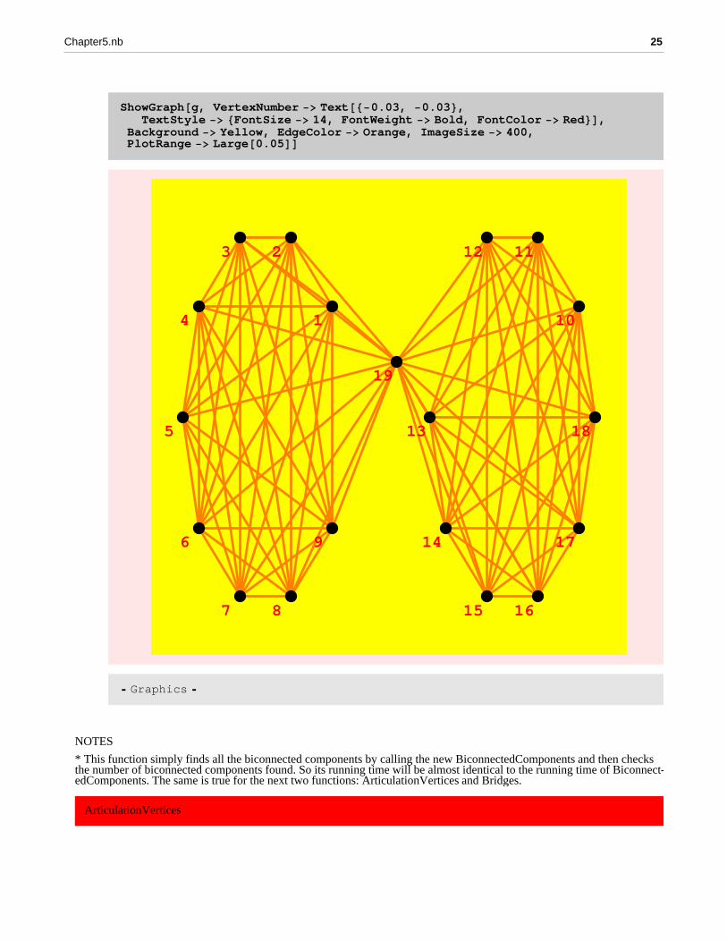
ShowGraph@g, VertexNumber -> Text@8-0.03, -0.03<,TextStyle -> 8FontSize -> 14, FontWeight -> Bold, FontColor -> Red<D,

Background -> Yellow, EdgeColor -> Orange, ImageSize -> 400,PlotRange -> Large@0.05DD

1

23

4

5

6

7 8

9

10

1112

13

14

15 16

17

18

19

� Graphics �

NOTES

* This function simply finds all the biconnected components by calling the new BiconnectedComponents and then checks the number of biconnected components found. So its running time will be almost identical to the running time of Biconnect-edComponents. The same is true for the next two functions: ArticulationVertices and Bridges.

ArticulationVertices

Chapter5.nb 25

? ArticulationVertices

ArticulationVertices@gD gives a list of all articulation vertices ingraph g. These are vertices whose removal will disconnect the graph.

g = Star@20D;ArticulationVertices@gD820<ArticulationVertices@CompleteGraph@10DD8<

Bridges

? Bridges

Bridges@gD gives a list of the bridges of graph g,that is, the edges whose removal disconnects the graph.

Bridges@RandomTree@10DD881, 6<, 84, 7<, 87, 9<, 85, 9<, 85, 10<, 82, 3<, 83, 8<, 88, 10<, 81, 10<<g = GridGraph@10, 10D;Bridges@gD8<Bridges@s = AddEdges@GraphUnion@Wheel@5D, Wheel@7DD, 8885, 6<<<DD885, 6<<

26 Chapter5.nb

ShowGraph@s, VertexNumber -> On, PlotRange -> Large@0.05DD

1

2

3

45

67

8

9 10

1112

� Graphics �

EdgeConnectivity

? EdgeConnectivity

EdgeConnectivity@gD gives the minimum numberof edges whose deletion from graph g disconnects it.

EdgeConnectivity@ GridGraph@20, 5DD2

EdgeConnectivity@s = AddEdges@GraphUnion@Wheel@5D, Wheel@7DD, 8885, 6<<<DD1

Chapter5.nb 27

EdgeConnectivity@ RandomGraph@20, .3D D1

EdgeConnectivity@ RandomGraph@20, .5D D6

EdgeConnectivity@ RandomGraph@20, .7D D10

EdgeConnectivity @ CompleteGraph@10D D9

TIMING DISCUSSION

EdgeConnectivity is extremely slow because it calls NetworkFlow n times. 220 seconds for a 5 X 250 grid graph!! This needs substantial repair. The way to do EdgeConnectivity efficiently would be to implement the Stoer−Wagner algorithm. I should also implement preflow−push to speedup the NetworkFlow algorithm. I should then do a timing comparison of both algorithms.

The new implementation is faster than the old implementation, but this is no reason to gloat given that both implementa-tions are terribly slow.

TO DO

* Implement Stoer−Wagner algorithm for edge connectivity.

* Implement the pre−flow puch algorithm for Network flows.

gt = Table @RandomGraph@5 i, N@1 � H5 iLDD, 8i, 15<D;rt = Table @Timing@ EdgeConnectivity@ gt@@iDD D; D, 8i, 15<D880. Second, Null<, 80.047 Second, Null<, 80.047 Second, Null<,80.109 Second, Null<, 80.125 Second, Null<, 80.188 Second, Null<,80.25 Second, Null<, 80.469 Second, Null<, 80.453 Second, Null<,80.875 Second, Null<, 80.578 Second, Null<, 80.812 Second, Null<,80.938 Second, Null<, 81.031 Second, Null<, 81.063 Second, Null<<

28 Chapter5.nb

Map@V, gtD85, 10, 15, 20, 25, 30, 35, 40, 45, 50, 55, 60, 65, 70, 75<Map@M, gtD81, 6, 5, 10, 11, 13, 14, 26, 25, 36, 26, 40, 43, 44, 37<ListPlot@ Map@ #@@1, 1DD &, rtD, PlotJoined -> TrueD

2 4 6 8 10 12 14

0.2

0.4

0.6

0.8

1

� Graphics �

gt = Table @GridGraph@5, 5 iD, 8i, 10<D;rt = Table @Timing@ EdgeConnectivity@ gt@@iDD D; D, 8i, 10<D880.609 Second, Null<, 82.422 Second, Null<,85.578 Second, Null<, 810.078 Second, Null<, 816.453 Second, Null<,823.985 Second, Null<, 833.437 Second, Null<,842.672 Second, Null<, 854.828 Second, Null<, 895.625 Second, Null<<

Chapter5.nb 29

ListPlot@ Map@ #@@1, 1DD &, rtD, PlotJoined -> TrueD

4 6 8 10

20

40

60

80

� Graphics �

h = Table @DiscreteMath‘OldCombinatorica‘RandomGraph@i * 5, N@1 � 5 iDD, 8i, 5<D;Table @Timing@ DiscreteMath‘OldCombinatorica‘EdgeConnectivity@ h@@iDD D; D, 8i, 5<D

880.015 Second, Null<, 80.094 Second, Null<,80.625 Second, Null<, 82. Second, Null<, 84.375 Second, Null<<VertexConnectivity

? VertexConnectivity

VertexConnectivity@gD gives the minimum numberof vertices whose deletion from graph g disconnects it.

VertexConnectivity@ GridGraph@10, 3D D2

VertexConnectivity@ Star@30D D1

30 Chapter5.nb

VertexConnectivity@ CompleteGraph@4D D3

DiscreteMath‘OldCombinatorica‘VertexConnectivity @DiscreteMath‘OldCombinatorica‘CompleteGraph @ 4D D4

NOTES

* The convention is to define the vertex−connectivity of a complete graph of n vertices as n−1. Old Combinatorica does not get this right.

TIMING DISCUSSION

Vertex connectivity is too slow − that fact that the old version of this function is even slower is not a source of comfort. Calling Network Flow n times is a bad idea and an overkill. As I write in the comments for EdgeConnectivity, I should implement the Stoer−Wagner algorithm for both edge and vertex connectivity. Of course, I should also speed up network flow.

g = GridGraph@10, 4D; h = DiscreteMath‘OldCombinatorica‘GridGraph@10, 4D;Timing@ VertexConnectivity@ g D; D87.485 Second, Null<Timing@ DiscreteMath‘OldCombinatorica‘VertexConnectivity@ h D; D820.64 Second, Null<

VertexConnectivityGraph

? VertexConnectivityGraph

VertexConnectivityGraph@gD returns a directed graph thatcontains an edge corresponding to each vertex in g and in whichedge disjoint paths correspond to vertex disjoint paths in g.

NOTES

* This function was hidden in old Combinatorica. I think it produces interesting graphs and therefore have made the new function public. I have also tried to give the vertices a reasonable embedding that shows what transpired. The function produces directed graphs.

Chapter5.nb 31

ShowGraph@g = VertexConnectivityGraph@Wheel@10DD,VertexStyle -> Disc@0.025D, ImageSize -> 400D

� Graphics �

32 Chapter5.nb

ShowGraph@g = RandomTree@10DD

� Graphics �

NOTES

The following example also tries to show the use of relative headscaling for arrows. I thought this option would be very useful, but now I am skeptical. Look at the smallest edges − they seem not to have any arrow heads. That is only because their arrow heads are too small to be visible.

Chapter5.nb 33

ShowGraph@VertexConnectivityGraph@gD,HeadScaling -> Relative, ImageSize -> 400, VertexStyle -> Disc@0.015DD

� Graphics �

TIMING DISCUSSION

The above timing information shows that constructing the vertex connectivity graph takes virtually no time as compared to the computation of vertex connectivity itself: 0.02 s vc 26 s. So no significant improvement of VertexConnectivity will come from improving the construction of the vertex connectivity graph.

g = GridGraph@10, 4D; Timing@ VertexConnectivityGraph@gD; D80. Second, Null<

34 Chapter5.nb

TO DO

Both EdgeConnectivity and VertexConnectivity need to have options that will make the functions return a smallest edge−cut or smallest vertex−cut respectively.

Harary

? Harary

Harary@k, nD constructs the minimal k-connected graph on n vertices.

ShowGraph@Harary@3, 10DD

� Graphics �

Chapter5.nb 35

ShowGraph@Harary@7, 13DD

� Graphics �

CompleteQ@Harary@8, 9DDTrue

CompleteQ@Harary@10, 9DDCompleteQ@Harary@10, 9DD

TIMING DISCUSSION

Harary[n, k] seems to be linear both in n and in k. I need to look at the code more carefully to determine if this is indeed true. I am surprised that it is linear in n.

As can be seen from the timing results below, construction of the Harary graph using the old version of the function is faster than using the new version. This is because Harary makes a call to CirculantGraph and CirculantGraph is extremely fast in the old version because it uses extremely convenient in−built matrix/vector operations. I don’t think much can be done to improve the "new" version of Harary.

36 Chapter5.nb

rt = Table@Timing@ Harary@5, i * 10D;D, 8i, 20<D880. Second, Null<, 80.015 Second, Null<,80. Second, Null<, 80. Second, Null<, 80.016 Second, Null<,80. Second, Null<, 80.016 Second, Null<, 80.015 Second, Null<,80.016 Second, Null<, 80.015 Second, Null<, 80.016 Second, Null<,80.016 Second, Null<, 80.015 Second, Null<, 80.032 Second, Null<,80.015 Second, Null<, 80.031 Second, Null<, 80.016 Second, Null<,80.031 Second, Null<, 80.032 Second, Null<, 80.031 Second, Null<<ListPlot@ Map@#@@1, 1DD &, rtD, PlotJoined -> TrueD

5 10 15 20

0.005

0.01

0.015

0.02

0.025

0.03

� Graphics �

Table@Timing@ DiscreteMath‘OldCombinatorica‘Harary@5, i * 10D;D, 8i, 20<D880. Second, Null<, 80. Second, Null<, 80. Second, Null<, 80. Second, Null<,80. Second, Null<, 80. Second, Null<, 80. Second, Null<, 80. Second, Null<,80. Second, Null<, 80.016 Second, Null<, 80. Second, Null<, 80. Second, Null<,80. Second, Null<, 80.016 Second, Null<, 80. Second, Null<, 80. Second, Null<,80.015 Second, Null<, 80. Second, Null<, 80. Second, Null<, 80.016 Second, Null<<rt = Table@Timing@ Harary@5, i * 10D;D, 8i, 20<D880. Second, Null<, 80.016 Second, Null<,80. Second, Null<, 80. Second, Null<, 80.015 Second, Null<,80. Second, Null<, 80.016 Second, Null<, 80.015 Second, Null<,80.016 Second, Null<, 80.016 Second, Null<, 80.015 Second, Null<,80.016 Second, Null<, 80.016 Second, Null<, 80.031 Second, Null<,80.015 Second, Null<, 80.032 Second, Null<, 80.031 Second, Null<,80.016 Second, Null<, 80.031 Second, Null<, 80.031 Second, Null<<

Chapter5.nb 37

ListPlot@ Map@ #@@1, 1DD &, rtD, PlotJoined -> TrueD

5 10 15 20

0.005

0.01

0.015

0.02

0.025

0.03

� Graphics �

BUG

The old Harary is producing an error message here. How come?

Table@Timing@ DiscreteMath‘OldCombinatorica‘Harary@i * 5, 10D;D, 8i, 3, 20<DIdenticalQ

? IdenticalQ

IdenticalQ@g, hD yields True if graphsg and h have identical edge lists, even though theassociated graphics information need not be the same.

g = CompleteGraph@10D;IdenticalQ@g, CompleteGraph@10DDTrue

IdenticalQ@g, Wheel@10DDFalse

38 Chapter5.nb

g = AddEdges@g, 8881, 2<<<D;IdenticalQ@g, CompleteGraph@10DDFalse

IdenticalQ@CirculantGraph@10, Range@5DD, CompleteGraph@10DDTrue

IdenticalQ@RemoveMultipleEdges@CirculantGraph@10, Range@5DDD, CompleteGraph@10DDTrue

IdenticalQ@GraphDifference@Wheel@11D, AddVertices@Cycle@10D, 1 DD, Star@11DDTrue

g = GridGraph@100, 100D;Timing@ IdenticalQ@g, gD;D80.14 Second, Null<

TIMING DISCUSSION

The "new" version of IdenticalQ is quite fast − 10, 000 vertex−graphs in less than a second. Of course the old version of this function is also extremely fast since it involves comparing the two adjacency matrices.

IsomorphismQ

? IsomorphismQ

IsomorphismQ@g, h, pD tests if permutationp defines an isomorphism between graphs g and h.

Chapter5.nb 39

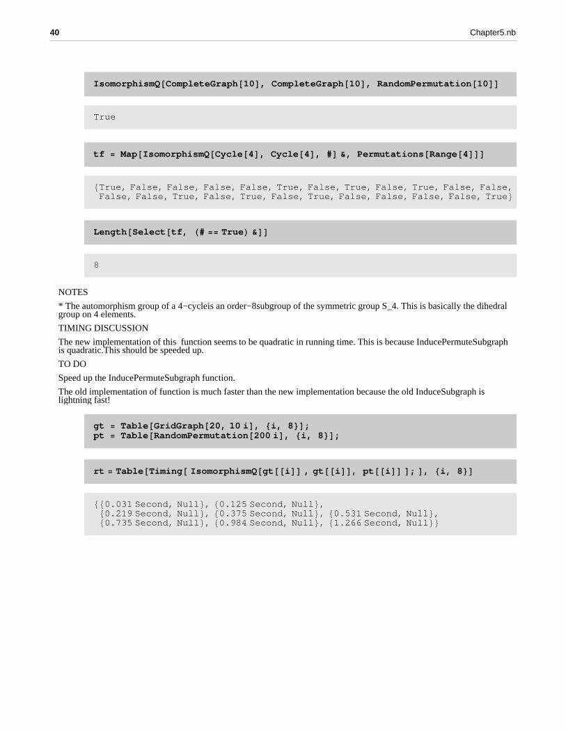
IsomorphismQ@CompleteGraph@10D, CompleteGraph@10D, RandomPermutation@10DDTrue

tf = Map@IsomorphismQ@Cycle@4D, Cycle@4D, #D &, Permutations@Range@4DDD8True, False, False, False, False, True, False, True, False, True, False, False,False, False, True, False, True, False, True, False, False, False, False, True<Length@Select@tf, H# == TrueL &DD8

NOTES

* The automorphism group of a 4−cycle is an order−8 subgroup of the symmetric group S_4. This is basically the dihedral group on 4 elements.

TIMING DISCUSSION

The new implementation of this function seems to be quadratic in running time. This is because InducePermuteSubgraph is quadratic.This should be speeded up.

TO DO

Speed up the InducePermuteSubgraph function.

The old implementation of function is much faster than the new implementation because the old InduceSubgraph is lightning fast!

gt = Table@GridGraph@20, 10 iD, 8i, 8<D;pt = Table@RandomPermutation@200 iD, 8i, 8<D;rt = Table@Timing@ IsomorphismQ@gt@@iDD , gt@@iDD, pt@@iDD D; D, 8i, 8<D880.031 Second, Null<, 80.125 Second, Null<,80.219 Second, Null<, 80.375 Second, Null<, 80.531 Second, Null<,80.735 Second, Null<, 80.984 Second, Null<, 81.266 Second, Null<<

40 Chapter5.nb

ListPlot@ Map@ #@@1, 1DD &, rtD, PlotJoined -> TrueD

2 3 4 5 6 7 8

0.2

0.4

0.6

0.8

1

1.2

� Graphics �

ht = Table@ DiscreteMath‘OldCombinatorica‘GridGraph@20, 10 iD, 8i, 8<D;rt = Table@ Timing@ DiscreteMath‘OldCombinatorica‘IsomorphismQ@

gt@@iDD, gt@@iDD, pt@@iDD D; D, 8i, 8<D880. Second, Null<, 80. Second, Null<, 80. Second, Null<, 80. Second, Null<,80. Second, Null<, 80. Second, Null<, 80. Second, Null<, 80. Second, Null<<

Isomorphism

? Isomorphism

Isomorphism@g, hD gives an isomorphism between graphs g and hif one exists. Isomorphism@g, h, AllD gives all isomorphismsbetween graphs g and h. Isomorphism@gD gives the automorphismgroup of g. This function takes an option Invariants -> 8f1,f2, ...<, where f1, f2, ... are functions that are used tocompute vertex invariants. These functions are used in the orderin which they are specified. The default value of Invariantsis 8DegreesOf2Neighborhood, NumberOf2Paths, Distances<.

Isomorphism@Wheel@10D, CompleteGraph@10DD8<

Chapter5.nb 41

Isomorphism@Wheel@5D, Wheel@5D, AllD881, 2, 3, 4, 5<, 81, 4, 3, 2, 5<, 82, 1, 4, 3, 5<, 82, 3, 4, 1, 5<,83, 2, 1, 4, 5<, 83, 4, 1, 2, 5<, 84, 1, 2, 3, 5<, 84, 3, 2, 1, 5<<Isomorphism@Star@5D, Star@5D, AllD881, 2, 3, 4, 5<, 81, 2, 4, 3, 5<, 81, 3, 2, 4, 5<, 81, 3, 4, 2, 5<, 81, 4, 2, 3, 5<,81, 4, 3, 2, 5<, 82, 1, 3, 4, 5<, 82, 1, 4, 3, 5<, 82, 3, 1, 4, 5<, 82, 3, 4, 1, 5<,82, 4, 1, 3, 5<, 82, 4, 3, 1, 5<, 83, 1, 2, 4, 5<, 83, 1, 4, 2, 5<, 83, 2, 1, 4, 5<,83, 2, 4, 1, 5<, 83, 4, 1, 2, 5<, 83, 4, 2, 1, 5<, 84, 1, 2, 3, 5<, 84, 1, 3, 2, 5<,84, 2, 1, 3, 5<, 84, 2, 3, 1, 5<, 84, 3, 1, 2, 5<, 84, 3, 2, 1, 5<<Isomorphism@Wheel@10D, Star@10DD8<Isomorphism@Cycle@10D, Cycle@10D, AllD881, 2, 3, 4, 5, 6, 7, 8, 9, 10<, 81, 10, 9, 8, 7, 6, 5, 4, 3, 2<,82, 1, 10, 9, 8, 7, 6, 5, 4, 3<, 82, 3, 4, 5, 6, 7, 8, 9, 10, 1<,83, 2, 1, 10, 9, 8, 7, 6, 5, 4<, 83, 4, 5, 6, 7, 8, 9, 10, 1, 2<,84, 3, 2, 1, 10, 9, 8, 7, 6, 5<, 84, 5, 6, 7, 8, 9, 10, 1, 2, 3<,85, 4, 3, 2, 1, 10, 9, 8, 7, 6<, 85, 6, 7, 8, 9, 10, 1, 2, 3, 4<,86, 5, 4, 3, 2, 1, 10, 9, 8, 7<, 86, 7, 8, 9, 10, 1, 2, 3, 4, 5<,87, 6, 5, 4, 3, 2, 1, 10, 9, 8<, 87, 8, 9, 10, 1, 2, 3, 4, 5, 6<,88, 7, 6, 5, 4, 3, 2, 1, 10, 9<, 88, 9, 10, 1, 2, 3, 4, 5, 6, 7<,89, 8, 7, 6, 5, 4, 3, 2, 1, 10<, 89, 10, 1, 2, 3, 4, 5, 6, 7, 8<,810, 1, 2, 3, 4, 5, 6, 7, 8, 9<, 810, 9, 8, 7, 6, 5, 4, 3, 2, 1<<

NOTES

* The above is the automorphism group of a 10−cycle. This is isomorphic to the dihedral group on 10 symbols.

TIMING DISCUSSION

The isomorphism function is extremely slow − the newer version of the function seems slower than the older (already slow) function. This function, needs major repair. It would be very nice to add a variety of heuristics to this function that help it prune the search space quickly. Clearly, Backtrack, as it is does not suffice. Brendan McKay’s Nauty specializes in graph isomorphism − I should look that up and see how it does what it does.

g = Table@Cycle@iD, 8i, 10, 20, 2<D; h = Table@Cycle@iD, 8i, 10, 20, 2<D;Table@Timing@ Isomorphism@g@@iDD, g@@iDD, AllD;D, 8i, 6<D$Aborted

42 Chapter5.nb

Table@Timing@DiscreteMath‘OldCombinatorica‘Isomorphism@h@@iDD, h@@iDD, AllD; D, 8i, 6<D

880. Second, Null<, 80.015 Second, Null<, 80. Second, Null<,80. Second, Null<, 80. Second, Null<, 80. Second, Null<<NOTES

* Now the new Isomorphism also yields the automorphism group if called with a single graph.

Isomorphism@Cycle@5DD881, 2, 3, 4, 5<, 81, 5, 4, 3, 2<, 82, 1, 5, 4, 3<, 82, 3, 4, 5, 1<, 83, 2, 1, 5, 4<,83, 4, 5, 1, 2<, 84, 3, 2, 1, 5<, 84, 5, 1, 2, 3<, 85, 1, 2, 3, 4<, 85, 4, 3, 2, 1<<Isomorphism@Path@5DD881, 2, 3, 4, 5<, 85, 4, 3, 2, 1<<Isomorphism@t = RandomTree@7DD881, 2, 3, 4, 5, 6, 7<, 81, 7, 3, 4, 5, 6, 2<<

Chapter5.nb 43

ShowGraph@t, VertexNumber -> On, PlotRange -> Large@.1DD

1

2

3

4

5

6

7

� Graphics �

IsomorphicQ

? IsomorphicQ

IsomorphicQ@g, hD yields True if graphs g and h are isomorphic.This function takes an option Invariants -> 8f1, f2, ...<,where f1, f2, ... are functions that are used to computevertex invariants. These functions are used in the order inwhich they are specified. The default value of Invariantsis 8DegreesOf2Neighborhood, NumberOf2Paths, Distances<.

IsomorphicQ@Wheel@10D, Wheel@10DDTrue

44 Chapter5.nb

IsomorphicQ@CompleteGraph@8D, GraphJoin@CompleteGraph@4D, CompleteGraph@4DDDTrue

IsomorphicQ@ RandomTree@20D, CompleteGraph@20DDFalse

Equivalences

? Equivalences

Equivalences@g, hD lists the vertex equivalence classes between graphs gand h defined by their vertex degrees. Equivalences@gD lists thevertex equivalences for graph g defined by the vertex degrees.Equivalences@g, h, f1, f2, ...D and Equivalences@g, f1, f2, ...Dcan also be used, where f1, f2, ... are functions that computeother vertex invariants. It is expected that for each functionfi, the call fi@g, vD returns the corresponding invariant atvertex v in graph g. The functions f1, f2, ... are evaluatedin order, and the evaluation stops either when all functionshave been evaluated or when an empty equivalence class is found.

NOTES

* The example below shows that the first 9 vertices in Wheel[10], each of which has degree 3, cannot be mapped on to any vertex in CompleteGraph[10], while the 10th vertex in Wheel[10], which has degree 9, can be mapped on to any vertex in CompleteGraph[10].

Equivalences@Wheel@10D, CompleteGraph@10DD88<, 8<, 8<, 8<, 8<, 8<, 8<, 8<, 8<, 81, 2, 3, 4, 5, 6, 7, 8, 9, 10<<Equivalences@Path@10D, CompleteGraph@10DD88<, 8<, 8<, 8<, 8<, 8<, 8<, 8<, 8<, 8<<Equivalences@Path@10D, Path@10DD881, 10<, 82, 3, 4, 5, 6, 7, 8, 9<, 82, 3, 4, 5, 6, 7, 8, 9<,82, 3, 4, 5, 6, 7, 8, 9<, 82, 3, 4, 5, 6, 7, 8, 9<, 82, 3, 4, 5, 6, 7, 8, 9<,82, 3, 4, 5, 6, 7, 8, 9<, 82, 3, 4, 5, 6, 7, 8, 9<, 82, 3, 4, 5, 6, 7, 8, 9<, 81, 10<<

NOTES

Below I construct two non−isomorphic 8−vertex 3−regular graphs. The first of these these two graphs, has several triangles while the second graph is Hypercube[3], which is bipartite. Note that since Equivalences[g, h] pays attention only to vertex degrees it ends up concluding that every vertex in the first graph can be mapped on to every vertex in the second graph. Looking at the adjacency matrix of the squares of these graphs quickly resolves the confusion and

Chapter5.nb 45

NOTES

Below I construct two non−isomorphic 8−vertex 3−regular graphs. The first of these these two graphs, has several triangles while the second graph is Hypercube[3], which is bipartite. Note that since Equivalences[g, h] pays attention only to vertex degrees it ends up concluding that every vertex in the first graph can be mapped on to every vertex in the second graph. Looking at the adjacency matrix of the squares of these graphs quickly resolves the confusion and

g = GraphUnion@ Cycle@4D, Cycle@4DD; ShowGraph@g, VertexNumber -> OnD

1

2

3

4

5

6

7

8

� Graphics �

g = AddEdges@g, 8 881, 5<<, 882, 4<<, 886, 8<<, 883, 7<< <D;

46 Chapter5.nb

ShowGraph@g, VertexNumber -> On, PlotRange -> Large@0.1DD

1

2

3

4

5

6

7

8

� Graphics �

DegreeSequence@ g D83, 3, 3, 3, 3, 3, 3, 3<

Chapter5.nb 47

ShowGraph@h = Hypercube@ 3 D D

� Graphics �

DegreeSequence@ h D83, 3, 3, 3, 3, 3, 3, 3<Equivalences@g, h D881, 2, 3, 4, 5, 6, 7, 8<, 81, 2, 3, 4, 5, 6, 7, 8<,81, 2, 3, 4, 5, 6, 7, 8<, 81, 2, 3, 4, 5, 6, 7, 8<, 81, 2, 3, 4, 5, 6, 7, 8<,81, 2, 3, 4, 5, 6, 7, 8<, 81, 2, 3, 4, 5, 6, 7, 8<, 81, 2, 3, 4, 5, 6, 7, 8<<Isomorphism@g, h, AllD8<

48 Chapter5.nb

Equivalences@ GraphPower@g, 2D, GraphPower@h, 2DD881, 2, 3, 4, 5, 6, 7, 8<, 8<, 81, 2, 3, 4, 5, 6, 7, 8<,8<, 81, 2, 3, 4, 5, 6, 7, 8<, 8<, 81, 2, 3, 4, 5, 6, 7, 8<, 8<<

NOTES

* This is simply the beginnings of how I think Isomorphism can be improved. I think that using AllPairsShortestPaths is probably too costly a method to determine equivalences. It would definitely be faster to use the number of paths matrix for paths of some small constant length. This matrix can be computed by simple matrix multiplication, which will make the computation relatively fast. Also, the user should be allowed to play with Equivalences so that using different methods, the equivalences can be made more fine. Here is an example.

gm = Path@10D; gm2 = GraphPower@gm, 2D;Equivalences@gm2, gm2D881, 10<, 82, 9<, 83, 4, 5, 6, 7, 8<, 83, 4, 5, 6, 7, 8<, 83, 4, 5, 6, 7, 8<,83, 4, 5, 6, 7, 8<, 83, 4, 5, 6, 7, 8<, 83, 4, 5, 6, 7, 8<, 82, 9<, 81, 10<<

NOTE

* Notice that since we used the 2nd power of the adjacency matrix, we have finer equivalence classes. Similarly, the situation improves with the third power of the adjacency matrix. Finally, when we get to the 5th power of adjacency matrix, it is clear that there are only two candidate permutations that we need to try: identity and the path "flip". In this case, both are isomorphisms.

Equivalences@gm3 = GraphPower@gm, 3D, gm3D881, 10<, 82, 9<, 83, 8<, 84, 5, 6, 7<, 84, 5, 6, 7<,84, 5, 6, 7<, 84, 5, 6, 7<, 83, 8<, 82, 9<, 81, 10<<Equivalences@gm5 = GraphPower@gm, 5D, gm5D881, 10<, 82, 9<, 83, 8<, 84, 7<, 85, 6<, 85, 6<, 84, 7<, 83, 8<, 82, 9<, 81, 10<<Equivalences@Wheel@5DD881, 2, 3, 4<, 81, 2, 3, 4<, 81, 2, 3, 4<, 81, 2, 3, 4<, 85<<Equivalences@CompleteGraph@4DD881, 2, 3, 4<, 81, 2, 3, 4<, 81, 2, 3, 4<, 81, 2, 3, 4<<

Chapter5.nb 49

Automorphisms

? Automorphisms

Automorphisms@gD gives the automorphism group of the graph g.

Automorphisms@Star@4DD881, 2, 3, 4<, 81, 3, 2, 4<, 82, 1, 3, 4<, 82, 3, 1, 4<, 83, 1, 2, 4<, 83, 2, 1, 4<<

SelfComplementaryQ

? SelfComplementaryQ

SelfComplementaryQ@gD yields True if graph g is self-complementary, meaning it is isomorphic to its complement.

SelfComplementaryQ@Path@4DDTrue

SelfComplementaryQ@Cycle@5DDTrue

SelfComplementaryQ@Path@5DDFalse

FindCycle

? FindCycle

FindCycle@gD finds a list of vertices that define a cycle in graph g.

NOTES

* FindCycle needs to have an edge option that will cause the function to return the edges in a cycle. This option can then be carried over to ExtractCycles.

50 Chapter5.nb

ShowGraph@t = RandomGraph@10, .4D, VertexNumber -> On,VertexNumberColor -> Red, PlotRange -> Large@0.1D, Background -> LightBlueD

1

23

4

5

6

7 8

9

10

� Graphics �

FindCycle@tD84, 1, 3, 4<

Chapter5.nb 51

ShowGraph@t = AddEdges@RandomTree@10D, 8881, 10<<<D,VertexNumber -> On, PlotRange -> Large@0.05DD

12

3

4

5

6

7

8

9

10

� Graphics �

FindCycle@tD810, 1, 2, 6, 9, 4, 5, 3, 10<HighlightCycle@t_GraphD := Highlight@t, c = FindCycle@tD;8Table@Sort@8c@@iDD, c@@i + 1DD<D, 8i, Length@cD - 1<D<,

HighlightedEdgeColors -> 8Red<D �; UndirectedQ@tDHighlightCycle@t_GraphD := Highlight@t,c = FindCycle@tD; 8Table@8c@@iDD, c@@i + 1DD<, 8i, Length@cD - 1<D<,HighlightedEdgeColors -> 8Red<D

52 Chapter5.nb

ShowGraph@HighlightCycle@tD, VertexNumber -> OnD

12

3

4

5

6

7

8

9

10

� Graphics �

Chapter5.nb 53

ShowGraph@HighlightCycle@RandomGraph@10, .4DDD

� Graphics �

54 Chapter5.nb

ShowGraph@t = SetGraphOptions@GridGraph@5, 5D, EdgeDirection -> On,VertexNumber -> Text@8-0.03, -0.03<DD, PlotRange -> Large@0.07DD

1 2 3 4 5

6 7 8 9 10

11 12 13 14 15

16 17 18 19 20

21 22 23 24 25

� Graphics �

Chapter5.nb 55

ShowGraph@t =AddEdges@DeleteEdges@t, 8816, 17<, 817, 22<<D, 88817, 16<<, 8822, 17<<<D,VertexNumber -> On, PlotRange -> Large@0.1DD

1 2 3 4 5

6 7 8 9 10

11 12 13 14 15

16 17 18 19 20

21 22 23 24 25

� Graphics �

56 Chapter5.nb

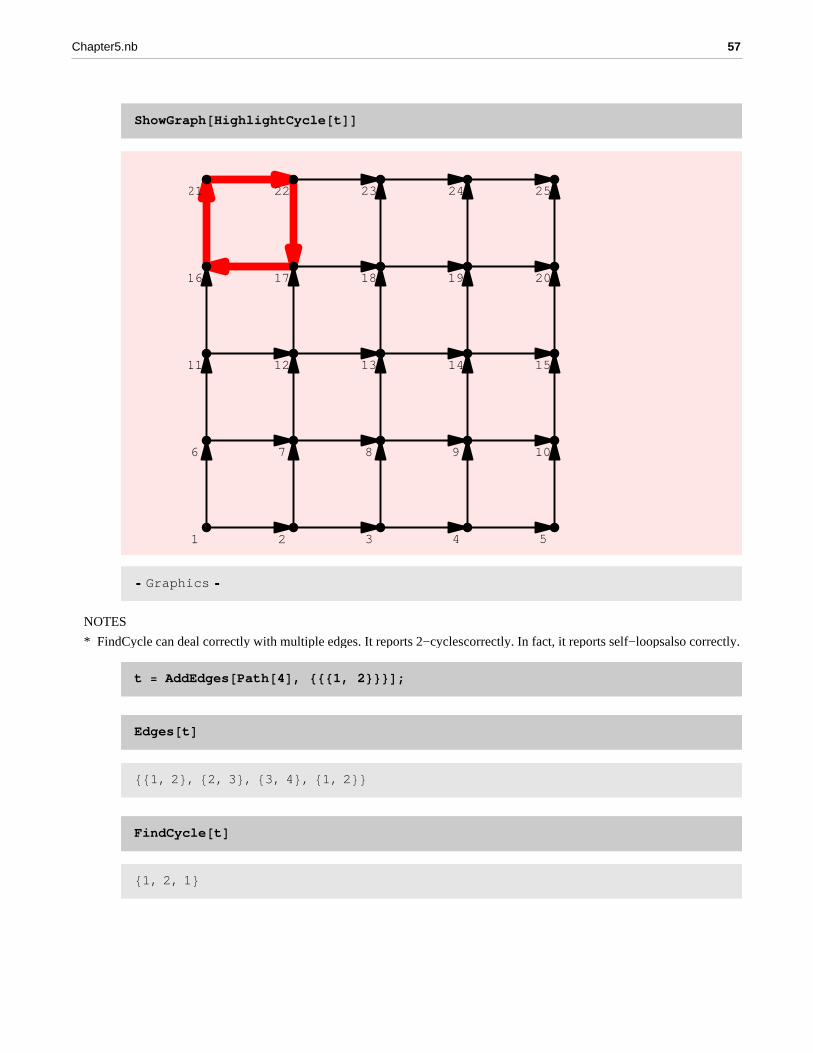
ShowGraph@HighlightCycle@tDD

1 2 3 4 5

6 7 8 9 10

11 12 13 14 15

16 17 18 19 20

21 22 23 24 25

� Graphics �

NOTES

* FindCycle can deal correctly with multiple edges. It reports 2−cycles correctly. In fact, it reports self−loops also correctly.

t = AddEdges@Path@4D, 8881, 2<<<D;Edges@tD881, 2<, 82, 3<, 83, 4<, 81, 2<<FindCycle@tD81, 2, 1<

Chapter5.nb 57

t = AddEdges@ Path@4D, 8 881, 1<< < D;FindCycle@ t D81, 1<

TIMING DISCUSSION

The plot of the table of timings for FindCyle on random graphs is quite strange − partly caused by the fact that the graphs are random and partly caused by the fact that the function stops as soon as it finds a cycle.

The plot of FindCycle timings for grid graphs is shown below. This is linear, but this is just because the function quickly finds 4−cycles in each of these graphs. The asymptotic running time of the function is definitely quadratic and this needs to be fixed.

The new version of FindCyle is faster than the old version, but the new version could be improved some more.

TO DO

Speed up FindCycle.

gt = Table@ RandomGraph@50 i, N@1 � H50 iLDD, 8i, 10<D;rt = Table@ Timing@ FindCycle@gt@@iDD D;D, 8i, 10<D880.016 Second, Null<, 80.047 Second, Null<,80.031 Second, Null<, 80.094 Second, Null<,80.031 Second, Null<, 80.156 Second, Null<, 80.313 Second, Null<,80.359 Second, Null<, 80.328 Second, Null<, 80.688 Second, Null<<ListPlot@ Map@ #@@1, 1DD &, rtD, PlotJoined -> TrueD

4 6 8 10

0.1

0.2

0.3

0.4

0.5

0.6

0.7

� Graphics �

58 Chapter5.nb

gt = Table@ GridGraph@20, 10 iD, 8i, 10<D;ct = Table@0, 810<D;rt = Table@ Timing@ct@@iDD = FindCycle@gt@@iDD D;D, 8i, 10<D880.015 Second, Null<, 80.031 Second, Null<,80.047 Second, Null<, 80.063 Second, Null<,80.078 Second, Null<, 80.109 Second, Null<, 80.11 Second, Null<,80.125 Second, Null<, 80.172 Second, Null<, 80.171 Second, Null<<ct

8839, 19, 20, 40, 39<, 839, 19, 20, 40, 39<,839, 19, 20, 40, 39<, 839, 19, 20, 40, 39<,839, 19, 20, 40, 39<, 839, 19, 20, 40, 39<, 839, 19, 20, 40, 39<,839, 19, 20, 40, 39<, 839, 19, 20, 40, 39<, 839, 19, 20, 40, 39<<ListPlot@ Map@ #@@1, 1DD &, rtD, PlotJoined -> TrueD

4 6 8 10

0.025

0.05

0.075

0.125

0.15

0.175

� Graphics �

ht =Table@DiscreteMath‘OldCombinatorica‘RandomGraph@50 i, N@1 � H50 iLDD, 8i, 5<D;

Chapter5.nb 59

rt = Table@Timing@ DiscreteMath‘OldCombinatorica‘FindCycle@ht@@iDD D; D, 8i, 5<D880.016 Second, Null<, 80.062 Second, Null<,80.188 Second, Null<, 80.281 Second, Null<, 80.797 Second, Null<<

AcyclicQ

? AcyclicQ

AcyclicQ@gD yields True if graph g is acyclic.

AcyclicQ@RandomTree@100DDTrue

AcyclicQ@GridGraph@10, 10DDFalse

AcyclicQ@SetGraphOptions@GridGraph@10, 10D, EdgeDirection -> OnDDTrue

TreeQ

? TreeQ

TreeQ@gD yields True if graph g is a tree.

TreeQ@Star@100DDTrue

$RecursionLimit = 10000;

60 Chapter5.nb

TreeQ@Path@100DDTrue

TreeQ@RandomTree@10DDTrue

TreeQ@CompleteGraph@10DDFalse

TreeQ@Wheel@10DDFalse

ExtractCycles

? ExtractCycles

ExtractCycles@gD gives a maximal list of edge-disjoint cycles in graph g.

ExtractCycles@Wheel@10DD889, 1, 2, 3, 4, 5, 6, 7, 8, 9<<cl = ExtractCycles@CompleteGraph@10DD889, 6, 8, 7, 9<, 89, 4, 8, 5, 9<, 87, 4, 6, 5, 7<, 89, 1, 8, 3, 9<, 89, 8, 2, 9<,87, 1, 6, 3, 7<, 87, 6, 2, 7<, 85, 1, 4, 3, 5<, 85, 4, 2, 5<, 83, 1, 2, 3<<

Chapter5.nb 61

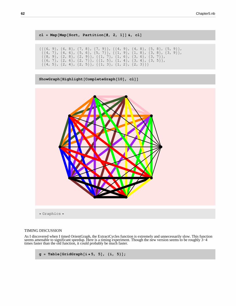
cl = Map@Map@Sort, Partition@#, 2, 1DD &, clD8886, 9<, 86, 8<, 87, 8<, 87, 9<<, 884, 9<, 84, 8<, 85, 8<, 85, 9<<,884, 7<, 84, 6<, 85, 6<, 85, 7<<, 881, 9<, 81, 8<, 83, 8<, 83, 9<<,888, 9<, 82, 8<, 82, 9<<, 881, 7<, 81, 6<, 83, 6<, 83, 7<<,886, 7<, 82, 6<, 82, 7<<, 881, 5<, 81, 4<, 83, 4<, 83, 5<<,884, 5<, 82, 4<, 82, 5<<, 881, 3<, 81, 2<, 82, 3<<<ShowGraph@Highlight@CompleteGraph@10D, clDD

� Graphics �

TIMING DISCUSSION

As I discovered when I timed OrientGraph, the ExtractCycles function is extremely and unnecessarily slow. This function seems amenable to significant speedup. Here is a timing experiment. Though the new version seems to be roughly 3−4 times faster than the old function, it could probably be much faster.

g = Table@GridGraph@i * 5, 5D, 8i, 5<D;

62 Chapter5.nb

Table@ Timing@ ExtractCycles@g@@iDDD; D, 8i, 5<D880.078 Second, Null<, 80.266 Second, Null<,80.594 Second, Null<, 81.125 Second, Null<, 81.797 Second, Null<<h = Table@DiscreteMath‘OldCombinatorica‘GridGraph@i * 5, 5D, 8i, 5<D;Table@ Timing@ DiscreteMath‘OldCombinatorica‘ExtractCycles@h@@iDDD; D, 8i, 5<D880.078 Second, Null<, 80.438 Second, Null<,81.203 Second, Null<, 82.672 Second, Null<, 84.969 Second, Null<<

DeleteCycle

? DeleteCycle

DeleteCycle@g, cD deletes a simple cycle c from graph g. c is specifiedas a sequence of vertices in which the first and last vertex areidentical. g can be directed or undirected. If g does not containc, it is returned unchanged, otherwise g is returned with c deleted.

NOTE

* This function should probably be able to delete several cycles in one shot.

Chapter5.nb 63

ShowGraph@DeleteCycle@CompleteGraph@10D, 81, 2, 3, 4, 5, 6, 7, 8, 9, 10, 1<DD

� Graphics �

IdenticalQ@DeleteCycle@Wheel@10D, 81, 2, 3, 4, 5, 6, 7, 8, 9, 1<D, Star@10DDTrue

TIMING DISCUSSION

Both versions of DeleteCycle are pretty fast and there is not much scope for improvement here.

g = GridGraph@30, 30D;Timing@ DeleteCycle@g, 81, 2, 3, 33, 32, 31, 1<D; D80.094 Second, Null<

64 Chapter5.nb

h = DiscreteMath‘OldCombinatorica‘GridGraph@30, 30D;Timing@DiscreteMath‘OldCombinatorica‘DeleteCycle@g, 81, 2, 3, 33, 32, 31, 1<D; D

80. Second, Null<Girth

? Girth

Girth@gD gives the length of the shortest cycle in a simple graph g.

NOTES

* The new Girth should probably return a cycle that realizes thegirth. It might have been fun to have a construction of a graph with arbitrarily large girth AND arbitrarily large chromatic number. Nesetril and Rodl supposedly have a construc-tion that is not too complicated.

Girth@Wheel@10DD3

Girth@GridGraph@5, 5DD4

Girth@Cycle@10DD10

Chapter5.nb 65

ShowGraph@t = AddEdges@Cycle@10D, 8881, 6<<<DD

� Graphics �

Girth@tD6

Girth@CompleteGraph@4, 4DD4

Girth@RandomTree@10DD¥

TIMING DISCUSSION

I need to look at the code of Girth to figure out what its asymptotic running time is. The plot below indicates that it is superlinear. I suspect it’s running time is cubic.

The new version of Girth is a shade faster than the older version of Girth. Can it be speeded up significantly?

66 Chapter5.nb

TIMING DISCUSSION

I need to look at the code of Girth to figure out what its asymptotic running time is. The plot below indicates that it is superlinear. I suspect it’s running time is cubic.

The new version of Girth is a shade faster than the older version of Girth. Can it be speeded up significantly?

gt = Table@RandomGraph@i * 10, .4D, 8i, 1, 10<D;rt = Table @ Timing@ Girth@gt@@iDDD; D, 8i, 10<D880. Second, Null<, 80.016 Second, Null<,80.047 Second, Null<, 80.062 Second, Null<,80.094 Second, Null<, 80.156 Second, Null<, 80.188 Second, Null<,80.266 Second, Null<, 80.343 Second, Null<, 80.438 Second, Null<<ListPlot@ Map@ #@@1, 1DD &, rtD, PlotJoined -> TrueD

4 6 8 10

0.1

0.2

0.3

0.4

� Graphics �

ht = Table@DiscreteMath‘OldCombinatorica‘RandomGraph@i * 10, .4D, 8i, 1, 10<D;rt = Table @ Timing@DiscreteMath‘OldCombinatorica‘Girth@ht@@iDDD; D, 8i, 10<D880. Second, Null<, 80.031 Second, Null<,80.031 Second, Null<, 80.063 Second, Null<,80.125 Second, Null<, 80.156 Second, Null<, 80.219 Second, Null<,80.281 Second, Null<, 80.375 Second, Null<, 80.438 Second, Null<<

OutDegree

Chapter5.nb 67

? OutDegree

OutDegree@g, nD returns the out-degree of vertexn in directed graph g. OutDegree@gD returns the sequenceof out-degrees of the vertices in directed graph g.

OutDegree@t = SetGraphOptions@GridGraph@5, 7D, EdgeDirection -> OnDD82, 2, 2, 2, 1, 2, 2, 2, 2, 1, 2, 2, 2, 2, 1,2, 2, 2, 2, 1, 2, 2, 2, 2, 1, 2, 2, 2, 2, 1, 1, 1, 1, 1, 0<ShowGraph@t, VertexNumber -> On, PlotRange -> Large@0.07DD

1 2 3 4 5

6 7 8 9 10

11 12 13 14 15

16 17 18 19 20

21 22 23 24 25

26 27 28 29 30

31 32 33 34 35

� Graphics �

OutDegree@SetGraphOptions@GraphUnion@10, CompleteGraph@1DD, EdgeDirection -> OnDD

80, 0, 0, 0, 0, 0, 0, 0, 0, 0<

68 Chapter5.nb

InDegree

? InDegree

InDegree@g, nD returns the in-degree of vertexn in directed graph g. InDegree@gD returns the sequenceof in-degrees of the vertices in directed graph g.

InDegree@SetGraphOptions@GridGraph@5, 5D, EdgeDirection -> OnDD80, 1, 1, 1, 1, 1, 2, 2, 2, 2, 1, 2, 2, 2, 2, 1, 2, 2, 2, 2, 1, 2, 2, 2, 2<

ReverseEdges

? ReverseEdges

ReverseEdges@gD flips the directions of all edges in a directed graph.

NOTES

* The new ReverseEdges has been created to help in writing the new InDegree function. This plays the same role that TransposeGraph played in the earlier implementation. Now I have gotten rid of TransposeGraph. Two questions I have are (1) Should the new ReverseEdges be public? (2) Should the new ReverseEdges be more general in the sense that any subset of edges should be reversible?

Chapter5.nb 69

ShowGraph@t = SetGraphOptions@GridGraph@5, 5D, EdgeDirection -> OnDD

� Graphics �

70 Chapter5.nb

ShowGraph@ReverseEdges@tDD

� Graphics �

EulerianQ

? EulerianQ

EulerianQ@gD yields True if the graph g is Eulerian, meaningthere exists a tour which includes each edge exactly once.

EulerianQ@CompleteGraph@9DDTrue

EulerianQ@Cycle@10DDTrue

Chapter5.nb 71

EulerianQ@t = GridGraph@5, 5DDFalse

ShowGraph@t, VertexNumber -> On, PlotRange -> Large@0.05DD

1 2 3 4 5

6 7 8 9 10

11 12 13 14 15

16 17 18 19 20

21 22 23 24 25

� Graphics �

72 Chapter5.nb

ShowGraph@t = DeleteVertices@t, 81, 5, 21, 25<D, VertexNumber -> OnD

1 2 3

4 5 6 7 8

9 10 11 12 13

14 15 16 17 18

19 20 21

� Graphics �

EulerianQ@tDFalse

Chapter5.nb 73

ShowGraph@t = DeleteEdges@t, 889, 10<, 816, 20<, 812, 13<, 82, 6<<DD

� Graphics �

EulerianQ@tDFalse

$RecursionLimit = 100000000000

100000000000

g = GridGraph@70, 70D;

74 Chapter5.nb

Timing@ EulerianQ@gD; D815.391 Second, Null<Timing@ ConnectedQ@gD; D815.141 Second, Null<

The new EulerianQ is reatively slow because of new ConnectedQ, as can be seen from the above example. When I replace the current ConnectedQ by the faster version, we should see a significant speedup in the new EulerianQ as well. It is quite amazing how slow the old version of EulerianQ is; I suppose I should not use that as a benchmark!

g = GridGraph@30, 30D;Timing@ EulerianQ@gD; D80.734 Second, Null<h = DiscreteMath‘OldCombinatorica‘GridGraph@30, 30D;Timing@ DiscreteMath‘OldCombinatorica‘EulerianQ@ h D; D89.953 Second, Null<

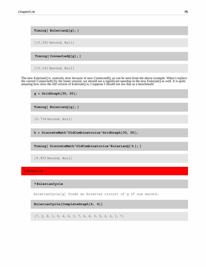
EulerianCycle

? EulerianCycle

EulerianCycle@gD finds an Eulerian circuit of g if one exists.

EulerianCycle@CompleteGraph@4, 4DD87, 2, 8, 1, 5, 4, 6, 3, 7, 4, 8, 3, 5, 2, 6, 1, 7<

Chapter5.nb 75

EulerianCycle@Hypercube@4DD816, 12, 8, 4, 1, 5, 6, 7, 8, 5, 9, 12, 11, 10, 9, 13,14, 15, 16, 13, 1, 2, 14, 10, 6, 2, 3, 15, 11, 7, 3, 4, 16<g = Table@Hypercube@iD, 8i, 3, 10<D;Table@Timing@ EulerianCycle@ g@@iDD D;D, 8i, 5<D880. Second, Null<, 80.062 Second, Null<,80.016 Second, Null<, 81.14 Second, Null<, 80.063 Second, Null<<Table@Timing@ ExtractCycles@ g@@iDD D;D, 8i, 5<D880.016 Second, Null<, 80.062 Second, Null<,80.625 Second, Null<, 81.047 Second, Null<, 818.609 Second, Null<<

The seemingly strange non−monotonic behaviour of the EulerianCycle function is because of the fact that Hypercubes with odd dimension are non−Eulerian, while the rest are. EulerianCycle starts by first checking if the given graph is Eulerian.

The bottleneck for this function also is ExtractCycles, when that is speeded up, EulerianCycle will be faster. Of course, the new version of the function is faster than the old version, but again that is no big consolation.

h = Table@DiscreteMath‘OldCombinatorica‘Hypercube@iD, 8i, 3, 7<D;Table@Timing@ DiscreteMath‘OldCombinatorica‘EulerianCycle@ h@@iDD D;D, 8i, 5<D880.016 Second, Null<, 80.063 Second, Null<,80.031 Second, Null<, 81.39 Second, Null<, 80.313 Second, Null<<

DeBruijnGraph

? DeBruijnGraph

DeBruijnGraph@m, nD constructs the n-dimensional De Bruijn graph with msymbols. DeBruijnGraph@alph, nD constructs the n-dimensional DeBruijn graph with symbols from alpha. In the latter form, thevertices of the graph are labeled by length Hn-1L strings on alph.

76 Chapter5.nb

ShowGraph@t = DeBruijnGraph@80, 1<, 4DD

80, 0, 0<80, 0, 1<

80, 1, 0<

80, 1, 1<

81, 0, 0<81, 0, 1<

81, 1, 0<

81, 1, 1<

� Graphics �

states = Map@FromCharacterCode, Map@H# + 48L &, Strings@80, 1<, 3DDD;

Chapter5.nb 77

ShowGraph@SetGraphOptions@t,Table@88i<, VertexLabel -> states@@iDD<, 8i, Length@statesD<DD,PlotRange -> 88-0.1, 1.2<, 8-0.1, 1.2<<D

80, 0, 0<80, 0, 1<

80, 1, 0<

80, 1, 1<

81, 0, 0<81, 0, 1<

81, 1, 0<

81, 1, 1<

� Graphics �

EulerianQ@tDTrue

states@@EulerianCycle@tDDD8000, 001, 010, 101, 011, 111, 111,110, 101, 010, 100, 001, 011, 110, 100, 000, 000<

In my view, it is more important to construct a DeBruijn graph, than a DeBruijn sequence − in fact it is simply one extra line of code to go from a DeBruijn graph to a DeBruijn sequence. So for now, I have replaced the function DeBruijnSe-quence by the new DeBruijnGraph. Of course we could always have both the graph and the sequence function.

Along with the DeBruijn graph and Hypercube, we might also consider other interconnection networks like the shuffle−exchange, butterfly network etc.

78 Chapter5.nb

Table@Timing@ DeBruijnGraph@ 80, 1<, iD;D, 8i, 3, 10<D880.015 Second, Null<, 80. Second, Null<,80.016 Second, Null<, 80.047 Second, Null<, 80.093 Second, Null<,80.266 Second, Null<, 81. Second, Null<, 84.031 Second, Null<<Table@Timing@ DeBruijnGraph@ 2, iD;D, 8i, 3, 10<D880. Second, Null<, 80.016 Second, Null<,80. Second, Null<, 80.016 Second, Null<, 80.062 Second, Null<,80.219 Second, Null<, 80.828 Second, Null<, 83.328 Second, Null<<

We are able to constuct a 10−dimensional DeBruijn graph (with 1024 vertices) in 4.29 seconds − not bad − is there scope for improvement?

HamiltonianCycle

? HamiltonianCycle

HamiltonianCycle@gD finds a Hamiltonian cycle in graph g if one exists.HamiltonianCycle@g, AllD gives all Hamiltonian cycles of graph g.

HamiltonianCycle@CompleteGraph@3, 3D, AllD881, 4, 2, 5, 3, 6, 1<, 81, 4, 2, 6, 3, 5, 1<, 81, 4, 3, 5, 2, 6, 1<,81, 4, 3, 6, 2, 5, 1<, 81, 5, 2, 4, 3, 6, 1<, 81, 5, 2, 6, 3, 4, 1<,81, 5, 3, 4, 2, 6, 1<, 81, 5, 3, 6, 2, 4, 1<, 81, 6, 2, 4, 3, 5, 1<,81, 6, 2, 5, 3, 4, 1<, 81, 6, 3, 4, 2, 5, 1<, 81, 6, 3, 5, 2, 4, 1<<

Chapter5.nb 79

ShowGraph@t = RegularGraph@4, 7D, VertexNumber -> OnD

1

2

3

4

5

6

7

� Graphics �

HamiltonianCycle@tD81, 2, 5, 6, 3, 7, 4, 1<HamiltonianCycle@AddEdges@GridGraph@5, 5D, 8881, 25<<<DD81, 2, 3, 4, 5, 10, 9, 8, 7, 6, 11, 12, 13,14, 15, 20, 19, 18, 17, 16, 21, 22, 23, 24, 25, 1<HamiltonianCycle@ GridGraph@5, 5D D8<

80 Chapter5.nb

g = Table@ GridGraph @i, iD, 8i, 3, 6<D;Table @ Timing@ HamiltonianCycle@ g@@iDD D; D, 8i, 4<D880.016 Second, Null<, 80.016 Second, Null<,825.265 Second, Null<, 819.922 Second, Null<<h = Table @ DiscreteMath‘OldCombinatorica‘GridGraph@i, iD, 8i, 3, 6<D;Table @Timing@ DiscreteMath‘OldCombinatorica‘HamiltonianCycle@ h@@iDD D; D, 8i, 4<D

880.016 Second, Null<, 80.016 Second, Null<,825.359 Second, Null<, 819.812 Second, Null<<There is virtually no difference between the running times of the old version and the new version of Hamiltonian Cycle. Again, I think this is a candidate for improvement.

SetEdgeWeights

? SetEdgeWeights

SetEdgeWeights@gD assigns random real weights in the range @0, 1Dto edges in g. SetWeights accepts options WeightingFunctionand WeightRange. WeightingFunction can take values Random,RandomInteger, Euclidean, LNorm@nD for non-negative n, or anypure function that takes as input two points. WeightRange canbe an integer range or a real range. The default value forWeightingFunction is Random and the default value for WeightRangeis @0, 1D. SetEdgeWeights@g, eD assigns edge weights to theedges in the edge list e. The options WeightingFunction andWeightRange apply. SetEdgeWeights@g, wD assigns the weights in theweight list w to the edges of g. SetEdgeWeights@g, e, wD assignsthe weights in the weight list w to the edges in edge list e.

This function assigns random weights to edges or vertices of a graph.

Chapter5.nb 81

Edges@SetEdgeWeights@GridGraph@5, 5DD, EdgeWeightD8881, 2<, 0.616363<, 882, 3<, 0.242657<, 883, 4<, 0.0951651<,884, 5<, 0.174373<, 886, 7<, 0.308184<, 887, 8<, 0.228384<, 888, 9<, 0.869308<,889, 10<, 0.317166<, 8811, 12<, 0.0589049<, 8812, 13<, 0.947536<,8813, 14<, 0.784791<, 8814, 15<, 0.34625<, 8816, 17<, 0.956441<,8817, 18<, 0.841366<, 8818, 19<, 0.203512<, 8819, 20<, 0.68216<,8821, 22<, 0.516524<, 8822, 23<, 0.0789837<, 8823, 24<, 0.0110615<,8824, 25<, 0.108073<, 881, 6<, 0.0675505<, 882, 7<, 0.49902<,883, 8<, 0.0746715<, 884, 9<, 0.393005<, 885, 10<, 0.451187<,886, 11<, 0.256363<, 887, 12<, 0.979506<, 888, 13<, 0.218632<,889, 14<, 0.143003<, 8810, 15<, 0.0279786<, 8811, 16<, 0.110199<,8812, 17<, 0.901465<, 8813, 18<, 0.084098<, 8814, 19<, 0.0804427<,8815, 20<, 0.325408<, 8816, 21<, 0.555215<, 8817, 22<, 0.127657<,8818, 23<, 0.239077<, 8819, 24<, 0.121896<, 8820, 25<, 0.873055<<Edges@SetEdgeWeights@GridGraph@5, 5D,

WeightingFunction -> RandomInteger, WeightRange -> 810, 20<D, EdgeWeightD8881, 2<, 14<, 882, 3<, 13<, 883, 4<, 15<, 884, 5<, 17<, 886, 7<, 14<,887, 8<, 12<, 888, 9<, 13<, 889, 10<, 14<, 8811, 12<, 17<, 8812, 13<, 20<,8813, 14<, 12<, 8814, 15<, 15<, 8816, 17<, 15<, 8817, 18<, 20<, 8818, 19<, 14<,8819, 20<, 12<, 8821, 22<, 11<, 8822, 23<, 15<, 8823, 24<, 19<, 8824, 25<, 18<,881, 6<, 17<, 882, 7<, 17<, 883, 8<, 10<, 884, 9<, 16<, 885, 10<, 11<,886, 11<, 14<, 887, 12<, 16<, 888, 13<, 19<, 889, 14<, 18<, 8810, 15<, 10<,8811, 16<, 12<, 8812, 17<, 15<, 8813, 18<, 11<, 8814, 19<, 17<, 8815, 20<, 17<,8816, 21<, 18<, 8817, 22<, 17<, 8818, 23<, 19<, 8819, 24<, 13<, 8820, 25<, 12<<Edges@SetEdgeWeights@GridGraph@5, 5D,

WeightingFunction -> Random, WeightRange -> 8-10, 10<D, EdgeWeightD8881, 2<, -6.03332<, 882, 3<, -1.85982<, 883, 4<, -2.73121<, 884, 5<, 3.06176<,886, 7<, -6.96123<, 887, 8<, -8.14157<, 888, 9<, 4.77624<, 889, 10<, -1.01041<,8811, 12<, 6.59344<, 8812, 13<, -9.27523<, 8813, 14<, -0.551626<,8814, 15<, -5.58674<, 8816, 17<, -5.45018<, 8817, 18<, -1.82038<,8818, 19<, -5.43148<, 8819, 20<, 5.90203<, 8821, 22<, -9.33851<,8822, 23<, -5.2686<, 8823, 24<, 0.855272<, 8824, 25<, -5.7657<,881, 6<, -7.4562<, 882, 7<, -9.77859<, 883, 8<, -5.48283<, 884, 9<, -9.96557<,885, 10<, 8.57712<, 886, 11<, 2.08123<, 887, 12<, 7.24838<, 888, 13<, -3.02733<,889, 14<, 5.53835<, 8810, 15<, 0.222798<, 8811, 16<, -7.52786<,8812, 17<, 7.98309<, 8813, 18<, 8.94491<, 8814, 19<, -0.501968<,8815, 20<, 3.02376<, 8816, 21<, 3.56983<, 8817, 22<, 4.39509<,8818, 23<, -8.68159<, 8819, 24<, -1.54476<, 8820, 25<, 7.6678<<Edges@SetEdgeWeights@GridGraph@3, 3D,

WeightingFunction -> EuclideanD, EdgeWeightD8881, 2<, 1.<, 882, 3<, 1.<, 884, 5<, 1.<, 885, 6<, 1.<, 887, 8<, 1.<, 888, 9<, 1.<,881, 4<, 1.<, 882, 5<, 1.<, 883, 6<, 1.<, 884, 7<, 1.<, 885, 8<, 1.<, 886, 9<, 1.<<

82 Chapter5.nb

H*GetEdgeWeights@SetEdgeWeights@GridGraph@3, 3D, WeightingFunction->L@1DDD*L8L@1D@81., 1.<, 82., 1.<D, L@1D@82., 1.<, 83., 1.<D, L@1D@81., 2.<, 82., 2.<D,L@1D@82., 2.<, 83., 2.<D, L@1D@81., 3.<, 82., 3.<D, L@1D@82., 3.<, 83., 3.<D,L@1D@81., 1.<, 81., 2.<D, L@1D@82., 1.<, 82., 2.<D, L@1D@83., 1.<, 83., 2.<D,L@1D@81., 2.<, 81., 3.<D, L@1D@82., 2.<, 82., 3.<D, L@1D@83., 2.<, 83., 3.<D<GetEdgeWeights@SetEdgeWeights@RandomGraph@10, .3D, WeightingFunction -> EuclideanDD

81.90211, 1.17557, 1.61803, 0.618034, 0.618034, 1.17557,1.90211, 1.17557, 0.618034, 1.61803, 1.90211, 1.61803, 1.17557<

SetVertexWeights

? SetVertexWeights

SetVertexWeights@gD assigns random real non-negative weights to verticesin g. SetVertexWeights@g, Random, type, rangeD assigns randomweights of specified type in the specified range to verticesin g. SetVertexWeights@g, wD assigns the weights in weightlist w to the vertices in g. SetVertexWeights@g, v, wD assignsthe weights in weight list w to the vertices in vertex list v.

*BUG: SetVertexWeights should have the same syntax as setEdgeWeights.

GetVertexWeights@SetVertexWeights@GridGraph@3, 3D, Random, Integer, 810, 20<DD

820, 16, 14, 11, 19, 10, 11, 13, 11<GetVertexWeights@SetVertexWeights@GridGraph@3, 3DDD80.611132, 0.160093, 0.110834, 0.764982,0.543582, 0.661074, 0.0361625, 0.371977, 0.0923942<

GetEdgeWeights

? GetEdgeWeights

GetEdgeWeights@gD returns the list of weights of the edges of g.

Chapter5.nb 83

g = SetEdgeWeights@GridGraph@5, 5D,WeightingFunction -> RandomInteger, WeightRange -> 80, 10<D;

GetEdgeWeights@gD82, 10, 6, 8, 5, 6, 2, 3, 6, 2, 6, 10, 1, 2, 8, 6, 5, 4, 10,2, 5, 10, 4, 3, 10, 10, 5, 6, 1, 3, 1, 6, 0, 4, 2, 7, 8, 7, 4, 3<

GetVertexWeights

? GetVertexWeights

GetVertexWeights@gD returns the list of weights of vertices of g.

GetVertexWeights@gD80, 0, 0, 0, 0, 0, 0, 0, 0, 0, 0, 0, 0, 0, 0, 0, 0, 0, 0, 0, 0, 0, 0, 0, 0<g = SetVertexWeights@g, Random, Integer, 8100, 200<D;GetVertexWeights@gD8178, 150, 186, 129, 156, 103, 107, 187, 118, 119, 131, 150,149, 178, 158, 149, 189, 119, 130, 197, 157, 162, 121, 199, 130<

CostOfPath

? CostOfPath

CostOfPath@g, pD sums up the weightsof the edges in graph g defined by the path p.

g = SetEdgeWeights@GridGraph@4, 4D,WeightingFunction -> RandomInteger, WeightRange -> 81, 5<D

�Graph:<24, 16, Undirected>�

84 Chapter5.nb

CostOfPath@g, 81, 2, 3, 4, 8, 12<D17

CostOfPath@g, 81, 2, 3, 4, 5, 6, 7, 8, 9, 10<D¥

TravelingSalesman

? TravelingSalesman

TravelingSalesman@gD finds theoptimal traveling salesman tour in graph g.

g = SetEdgeWeights@Cycle@10D,WeightingFunction -> RandomInteger, WeightRange -> 81, 3<D

�Graph:<10, 10, Undirected>�

TravelingSalesman@gD81, 2, 3, 4, 5, 6, 7, 8, 9, 10, 1<GetEdgeWeights@g = SetEdgeWeights@CompleteGraph@4D,

WeightingFunction -> RandomInteger, WeightRange -> 81, 100<DD839, 97, 13, 22, 71, 70<TravelingSalesman@gD81, 2, 3, 4, 1<

Chapter5.nb 85

GetEdgeWeights@g = SetEdgeWeights@Wheel@6D, WeightingFunction -> EuclideanDD81., 1., 1., 1., 1., 1.17557, 1.17557, 1.17557, 1.17557, 1.17557<p = TravelingSalesman@gD81, 2, 3, 4, 5, 6, 1<CostOfPath@g, pD6.70228

CostOfPath@g, 81, 2, 4, 3, 5, 6, 1<D¥

CostOfPath@g, 81, 2, 6, 3, 4, 5, 1<D6.70228

g = Table@SetEdgeWeights@CompleteGraph@iD,WeightingFunction -> RandomInteger, WeightRange -> 81, 100<D, 8i, 5, 8<D;

Table@ Timing@ TravelingSalesman@ g@@iDD D; D, 8i, 4<D880.078 Second, Null<, 80.829 Second, Null<,86.171 Second, Null<, 832.36 Second, Null<<

HamiltonianCycle and TravelingSalesman are very similar functions and any ideas for speeding up one can be applied to the other. For TravelingSalesman, there are different heuristics that can be used.

TriangleInequalityQ

? TriangleInequalityQ

TriangleInequalityQ@gD yields True if the weights assignedto the edges of graph g satisfy the triangle inequality.

86 Chapter5.nb

I don’t see this function used very much and so this is another candidate for deletion. I also wonder if I can implement this more efficiently − I simply construct a matrix of edge weights and then use the old code.

GetEdgeWeights@g = SetEdgeWeights@GridGraph@2, 2DDD80.40471, 0.0566561, 0.153345, 0.949391<TriangleInequalityQ@gDTrue

The above function returns true because there are no triangle in the grid graph!

GetEdgeWeights@g = SetEdgeWeights@CompleteGraph@5DDD80.376732, 0.946457, 0.25188, 0.865293, 0.296289,0.62105, 0.696664, 0.737637, 0.0572121, 0.499154<TriangleInequalityQ@gDFalse

As expected, randomly chosen edge weights will typically not satisfy the triangle inequality.

Below I set weights in K_4 to satisfy the triangle inequality.

g = SetGraphOptions@CompleteGraph@4D,88881, 2<, 82, 3<, 83, 4<, 81, 4<<, EdgeWeight -> 1<,8882, 4<, 81, 3<<, EdgeWeight -> 1.5<<D�Graph:<6, 4, Undirected>�

TriangleInequalityQ@gDTrue

g = SetGraphOptions@g, EdgeDirection -> OnD�Graph:<6, 4, Directed>�

Chapter5.nb 87

TriangleInequalityQ@gDTrue

TravelingSalesmanBounds

? TravelingSalesmanBounds

TravelingSalesmanBounds@gD gives upper and lower boundson the minimum cost traveling salesman tour of graph g.

TravelingSalesmanBounds@Wheel@5DD817, 5<

TransitiveClosure

? TransitiveClosure

TransitiveClosure@gD finds the transitiveclosure of graph g, the supergraph of g that containsedge 8x, y< if and only if there is a path from x to y.

88 Chapter5.nb

ShowGraph@g = SetGraphOptions@GridGraph@4, 4D, EdgeDirection -> OnD,VertexNumber -> OnD

1 2 3 4

5 6 7 8

9 10 11 12

13 14 15 16

� Graphics �

Here is an attempt to make the edges in the orginal graph show up in a different color as compared to the new edges added during by transitive closure. It does not quite work as one would want because of "hidden" edges such as {1, 3}, {1, 4}, {1, 9}, amd {1, 13} that are added by transitive closure AND because of the order in which the edges are rendered.

Edges@gD881, 2<, 82, 3<, 83, 4<, 85, 6<, 86, 7<, 87, 8<, 89, 10<, 810, 11<,811, 12<, 813, 14<, 814, 15<, 815, 16<, 81, 5<, 82, 6<, 83, 7<, 84, 8<,85, 9<, 86, 10<, 87, 11<, 88, 12<, 89, 13<, 810, 14<, 811, 15<, 812, 16<<

Chapter5.nb 89

ShowGraph@gg = TransitiveClosure@gD,Append@Edges@gD, EdgeColor -> RedD, VertexNumber ® OnD

1 2 3 4

5 6 7 8

9 10 11 12

13 14 15 16

� Graphics �

Edges@ggD881, 2<, 81, 3<, 81, 4<, 81, 5<, 81, 6<, 81, 7<, 81, 8<, 81, 9<, 81, 10<,81, 11<, 81, 12<, 81, 13<, 81, 14<, 81, 15<, 81, 16<, 82, 3<, 82, 4<, 82, 6<,82, 7<, 82, 8<, 82, 10<, 82, 11<, 82, 12<, 82, 14<, 82, 15<, 82, 16<, 83, 4<,83, 7<, 83, 8<, 83, 11<, 83, 12<, 83, 15<, 83, 16<, 84, 8<, 84, 12<, 84, 16<,85, 6<, 85, 7<, 85, 8<, 85, 9<, 85, 10<, 85, 11<, 85, 12<, 85, 13<, 85, 14<,85, 15<, 85, 16<, 86, 7<, 86, 8<, 86, 10<, 86, 11<, 86, 12<, 86, 14<, 86, 15<,86, 16<, 87, 8<, 87, 11<, 87, 12<, 87, 15<, 87, 16<, 88, 12<, 88, 16<,89, 10<, 89, 11<, 89, 12<, 89, 13<, 89, 14<, 89, 15<, 89, 16<, 810, 11<,810, 12<, 810, 14<, 810, 15<, 810, 16<, 811, 12<, 811, 15<, 811, 16<,812, 16<, 813, 14<, 813, 15<, 813, 16<, 814, 15<, 814, 16<, 815, 16<<g = DiscreteMath‘OldCombinatorica‘GridGraph@10, 10D;Timing@ DiscreteMath‘OldCombinatorica‘TransitiveClosure@gD;D813.969 Second, Null<

90 Chapter5.nb

g = GridGraph@10, 10D;Timing@ TransitiveClosure@gD; D813.953 Second, Null<

As expected, the new TransitiveClosure is slower than the old TransitiveClosure because the new version converts edge lists into an adjacency matrix representation and then simply uses the old code. I might be able to do this faster by not going into adjacency matrix representation??

TransitveQ

? TransitiveQ

TransitiveQ@gD yields True if graph g defines a transitive relation.

ShowGraph@g = SetGraphOptions@RandomGraph@10, 0.3D, EdgeDirection -> OnD,VertexNumber -> OnD

1

23

4

5

6

7 8

9

10

� Graphics �

Chapter5.nb 91

TransitiveQ@gDFalse

TransitiveQ@TransitiveClosure@gDDTrue

TransitiveQ@SetGraphOptions@CompleteGraph@10D, EdgeDirection -> OnDDTrue

TransitiveQ@g = SetGraphOptions@CompleteGraph@3, 3, 3D, EdgeDirection -> OnDDTrue

92 Chapter5.nb

ShowGraph@gD

� Graphics �

ReflexiveQ

? ReflexiveQ

ReflexiveQ@gD yields True if the adjacencymatrix of g represents a reflexive binary relation.

ReflexiveQ@g = CompleteGraph@10DDFalse

g = AddEdges@g, Table@88i, i<<, 8i, 10<DD;

Chapter5.nb 93

ReflexiveQ@gDTrue

g = DeleteEdges@g, 881, 1<<D;ReflexiveQ@gDFalse

AntiSymmetricQ

? AntiSymmetricQ

AntiSymmetricQ@gD yields True if the adjacencymatrix of g represents an anti-symmetric binary relation.

94 Chapter5.nb

ShowGraph@g = SetGraphOptions@Wheel@20D, EdgeDirection -> OnDD

� Graphics �

AntiSymmetricQ@gDTrue

Chapter5.nb 95

ShowGraph@g = AddEdges@g, 8882, 1<<<DD

� Graphics �

AntiSymmetricQ@gDFalse

PartialOrderQ

? PartialOrderQ

PartialOrderQ@gD yields True if the binary relation definedby the adjacency matrix of graph g is a partial order,meaning it is transitive, reflexive, and anti-symmetric.

96 Chapter5.nb

PartialOrderQ@g = GridGraph@3, 3DDFalse

g = TransitiveClosure@gD;Edges@gD881, 1<, 81, 2<, 81, 3<, 81, 4<, 81, 5<, 81, 6<, 81, 7<, 81, 8<, 81, 9<,82, 2<, 82, 3<, 82, 4<, 82, 5<, 82, 6<, 82, 7<, 82, 8<, 82, 9<, 83, 3<,83, 4<, 83, 5<, 83, 6<, 83, 7<, 83, 8<, 83, 9<, 84, 4<, 84, 5<, 84, 6<,84, 7<, 84, 8<, 84, 9<, 85, 5<, 85, 6<, 85, 7<, 85, 8<, 85, 9<, 86, 6<,86, 7<, 86, 8<, 86, 9<, 87, 7<, 87, 8<, 87, 9<, 88, 8<, 88, 9<, 89, 9<<PartialOrderQ@gDTrue

TransitiveReduction

? TransitiveReduction

TransitiveReduction@gD finds the smallestgraph which has the same transitive closure as g.

Chapter5.nb 97

ShowGraph@TransitiveReduction@g = SetGraphOptions@GridGraph@4, 4D, EdgeDirection -> OnDDD

� Graphics �

98 Chapter5.nb

ShowGraph@g = TransitiveClosure@gDD

� Graphics �

Chapter5.nb 99

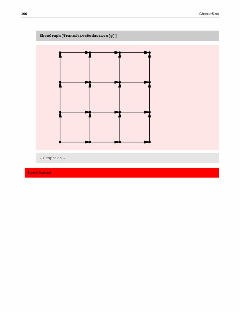
ShowGraph@TransitiveReduction@gDD

� Graphics �

HasseDiagram

100 Chapter5.nb

ShowGraph@s = MakeGraph@Subsets@4D, HHIntersection@#2, #1D === #1L && H#1 != #2LL &DD

� Graphics �

Chapter5.nb 101

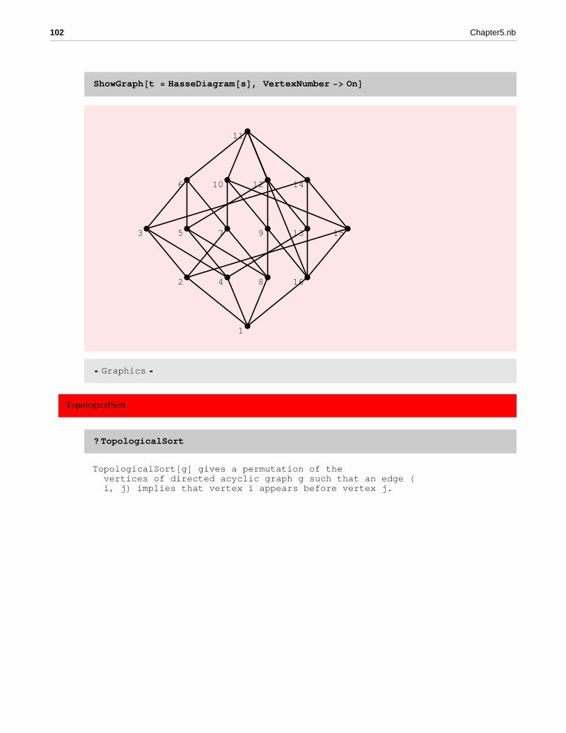
ShowGraph@t = HasseDiagram@sD, VertexNumber -> OnD

1

2

3

4

5

6

7

8

9

10

11

12

13

14

15

16

� Graphics �

TopologicalSort

? TopologicalSort

TopologicalSort@gD gives a permutation of thevertices of directed acyclic graph g such that an edge Hi, jL implies that vertex i appears before vertex j.

102 Chapter5.nb

ShowGraph@g = SetGraphOptions@GridGraph@5, 5D, EdgeDirection -> OnD,VertexNumber -> OnD

1 2 3 4 5

6 7 8 9 10

11 12 13 14 15

16 17 18 19 20

21 22 23 24 25

� Graphics �

Chapter5.nb 103

ShowGraph@HasseDiagram@gD, VertexNumber -> OnD

1

2

3

4

5

6

7

8

9

10

11

12

13

14

15

16

17

18

19

20

21

22

23

24

25

� Graphics �

TopologicalSort@gD81, 2, 6, 3, 7, 11, 4, 8, 12, 16, 5, 9,13, 17, 21, 10, 14, 18, 22, 15, 19, 23, 20, 24, 25<

104 Chapter5.nb

ShowGraph@g = AddEdges@DeleteEdges@g, 889, 10<<D, 88810, 9<<<DD

� Graphics �

TopologicalSort@gD81, 2, 6, 3, 7, 11, 4, 8, 12, 16, 5, 13,17, 21, 10, 18, 22, 9, 23, 14, 15, 19, 20, 24, 25<

Chapter5.nb 105

ShowGraph@g = MakeGraph@Range@12D, HMod@#2, #1D == 0L &D, VertexNumber -> OnD

1

2

3

4

5

6

7

8

9

10

11

12

� Graphics �

106 Chapter5.nb

ShowGraph@HasseDiagram@gD, VertexNumber -> OnD

1

2 3

4

5

6

7

8

9 10

11

12

� Graphics �

TopologicalSort@gD81, 2, 3, 5, 7, 11, 4, 6, 9, 10, 8, 12<

ChromaticPolynomial

? ChromaticPolynomial

ChromaticPolynomial@g, zD gives the chromatic polynomial PHzL of graphg, which counts the number of ways to color g with, at most, z colors.

g = CompleteGraph@5D;ChromaticPolynomial@g, zDH-4 + zL H-3 + zL H-2 + zL H-1 + zL z

Chapter5.nb 107

g = GraphUnion@10, CompleteGraph@1DD;ChromaticPolynomial@g, zDz10

ChromaticPolynomial@RandomTree@10D, zDH-1 + zL9 zg = DeleteEdges@CompleteGraph@5D, 881, 2<<D;ChromaticPolynomial@g, zDH-3 + zL H-2 + zL H-1 + zL z + H-4 + zL H-3 + zL H-2 + zL H-1 + zL z

ChromaticPolynomial@Cycle@5D, zD4 z - 10 z2 + 10 z3 - 5 z4 + z5

Table@8Timing@ DiscreteMath‘OldCombinatorica‘ChromaticPolynomial@DiscreteMath‘OldCombinatorica‘Cycle@iD, zD;D,

Timing@ChromaticPolynomial@Cycle@iD, zD;D<, 8i, 5, 10<D8880.047 Second, Null<, 80.015 Second, Null<<,880.063 Second, Null<, 80.047 Second, Null<<,880.109 Second, Null<, 80.109 Second, Null<<,880.235 Second, Null<, 80.203 Second, Null<<,880.484 Second, Null<, 80.422 Second, Null<<,881. Second, Null<, 80.844 Second, Null<<<

The speedup is not exciting! Clearly,more work is needed here.

Expand@wheelpoly@z_D = ChromaticPolynomial@Wheel@5D, zDD14 z - 31 z2 + 24 z3 - 8 z4 + z5

108 Chapter5.nb

Table@wheelpoly@zD, 8z, 1, 7<D80, 0, 6, 72, 420, 1560, 4410<

ChromaticNumber

? ChromaticNumber

ChromaticNumber@gD gives the chromatic number of the graph, whichis the fewest number of colors necessary to color the graph.

ChromaticNumber@Cycle@7DD3

ChromaticNumber@CompleteGraph@4, 5DD2

g = GridGraph@5, 5D;Timing@ ChromaticNumber@gD; D$Aborted

This function is hopelessly slow since it uses ChromaticPolynomials. We have to find other ways of finding an optimal coloring. I ran out of patience in trying the color the above 5X5 grid graph.

TwoColoring

? TwoColoring

TwoColoring@gD finds a two-coloring of graph g if g is bipartite. Itreturns as assignment of the labels 1 and 2 to vertices. Thisassignment is a valid coloring if and only the graph is bipartite.

Chapter5.nb 109

TwoColoring@t = RandomTree@20DD81, 2, 1, 1, 1, 1, 2, 1, 2, 2, 2, 1, 1, 2, 2, 1, 2, 2, 1, 1<$RecursionLimit = 100000;

TwoColoring@CompleteGraph@3, 3, 3DD81, 1, 1, 2, 2, 2, 2, 2, 2<g = Table@DiscreteMath‘OldCombinatorica‘GridGraph@i, iD, 8i, 10, 30, 10<D;h = Table@GridGraph@i, iD, 8i, 10, 30, 10<D;Table@8Timing@DiscreteMath‘OldCombinatorica‘TwoColoring@g@@iDDD;D,Timing@TwoColoring@h@@iDDD;D<, 8i, 3<D

8880.062 Second, Null<, 80.031 Second, Null<<,880.735 Second, Null<, 80.187 Second, Null<<,883.547 Second, Null<, 80.594 Second, Null<<<The new version of BreadthFirstTraversal returns levels of vertices as well. This can be used to obtain a one−line TwoColor-ing function. However, as can be seen from below, the new version is slightly slower, even though both versions are much faster than the old version of two coloring.

MyTC@ g_GraphD := Map@If@EvenQ@#D, 1, 2D &, BreadthFirstTraversal@g, 1, LevelDDMyTC@ t D81, 2, 1, 1, 1, 1, 2, 1, 2, 2, 2, 1, 1, 2, 2, 1, 2, 2, 1, 1<Table@ Timing@ MyTC@h@@iDDD; D, 8i, 3<D880.016 Second, Null<, 80.094 Second, Null<, 80.25 Second, Null<<

BipartiteQ

110 Chapter5.nb

? BipartiteQ

BipartiteQ@gD yields True if graph g is bipartite.

BipartiteQ@Wheel@10DDFalse

BipartiteQ@Star@10DDTrue

BipartiteQ@GridGraph@5, 5DDTrue

BipartiteQ@Cycle@5DDFalse

VertexColoring

? VertexColoring

VertexColoring@gD uses Brelaz’s heuristic to find a good, but notnecessarily minimal, vertex coloring of graph g. An optionAlgorithm that can take on the values Brelaz or Optimum isallowed. The setting Algorithm -> Brelaz is default, whilethe setting Algorithm -> Optimum forces the algorithm todo an exhaustive search and find an optimum vertex coloring.

VertexColoring@CompleteGraph@4DD81, 2, 3, 4<

Chapter5.nb 111

VertexColoring@GridGraph@10, 10DD81, 2, 1, 2, 1, 2, 1, 2, 1, 2, 2, 1, 2, 1, 2, 1, 2, 1, 2, 1, 1, 2, 1, 2, 1,2, 1, 2, 1, 2, 2, 1, 2, 1, 2, 1, 2, 1, 2, 1, 1, 2, 1, 2, 1, 2, 1, 2, 1, 2,2, 1, 2, 1, 2, 1, 2, 1, 2, 1, 1, 2, 1, 2, 1, 2, 1, 2, 1, 2, 2, 1, 2, 1, 2,1, 2, 1, 2, 1, 1, 2, 1, 2, 1, 2, 1, 2, 1, 2, 2, 1, 2, 1, 2, 1, 2, 1, 2, 1<c = VertexColoring@ g = Wheel@30D D81, 2, 1, 2, 1, 2, 1, 2, 1, 2, 1, 2, 1,2, 1, 2, 1, 2, 1, 2, 1, 2, 1, 2, 1, 2, 1, 2, 4, 3<p = Table@Flatten@Position@c, iD, 1D, 8i, Max@cD<D881, 3, 5, 7, 9, 11, 13, 15, 17, 19, 21, 23, 25, 27<,82, 4, 6, 8, 10, 12, 14, 16, 18, 20, 22, 24, 26, 28<, 830<, 829<<

112 Chapter5.nb

ShowGraph@ Highlight@g, pD D

� Graphics �

g = Table@DiscreteMath‘OldCombinatorica‘GridGraph@i, iD, 8i, 5, 30, 10<D;h = Table@GridGraph@i, iD, 8i, 5, 30, 10<D;Table@8Timing@DiscreteMath‘OldCombinatorica‘VertexColoring@g@@iDDD;D,Timing@VertexColoring@h@@iDDD;D<, 8i, 3<D

$Aborted

Originally, I used Steve’s code for this and was amazed at how slow both the new and the old implementations were (though the new implementation was just a little faster than the old implementation). I rewrote this function and the speedup is now significant significant!

g = ExactRandomGraph@30, 100D;

Chapter5.nb 113

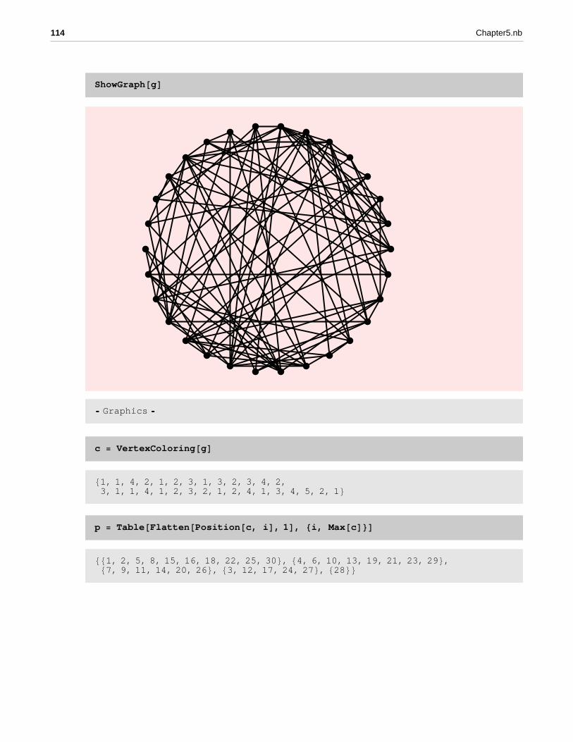
ShowGraph@gD

� Graphics �

c = VertexColoring@gD81, 1, 4, 2, 1, 2, 3, 1, 3, 2, 3, 4, 2,3, 1, 1, 4, 1, 2, 3, 2, 1, 2, 4, 1, 3, 4, 5, 2, 1<p = Table@Flatten@Position@c, iD, 1D, 8i, Max@cD<D881, 2, 5, 8, 15, 16, 18, 22, 25, 30<, 84, 6, 10, 13, 19, 21, 23, 29<,87, 9, 11, 14, 20, 26<, 83, 12, 17, 24, 27<, 828<<

114 Chapter5.nb

ShowGraph@Highlight@g, pDD

� Graphics �

EdgeColoring

? EdgeColoring

EdgeColoring@gD uses Brelaz’s heuristic to find agood, but not necessarily minimal, edge coloring of graph g.

EdgeColoring@Wheel@10DD81, 2, 3, 3, 2, 1, 4, 2, 5, 1, 6, 2, 7, 1, 8, 3, 9, 1<

Chapter5.nb 115

c = EdgeColoring@GridGraph@5, 5DD81, 2, 2, 3, 3, 1, 2, 1, 1, 1, 3, 2, 4, 3, 4, 2, 4, 3,1, 2, 2, 3, 1, 3, 2, 3, 1, 1, 3, 2, 4, 1, 4, 2, 4, 3, 1, 2, 1, 2<g = LineGraph@GridGraph@5, 5DD;p = Table@Flatten@Position@c, iD, 1D, 8i, 4<D881, 6, 8, 9, 10, 19, 23, 27, 28, 32, 37, 39<,82, 3, 7, 12, 16, 20, 21, 25, 30, 34, 38, 40<,84, 5, 11, 14, 18, 22, 24, 26, 29, 36<, 813, 15, 17, 31, 33, 35<<ShowGraph@Highlight@g, pD, VertexNumber -> OnD

1

2

3

4

5

6

7

8 9

10

11

12

13

14

15

16

17 18

19

20

21

22

23

24

25

26 27

28

29

30

31

32

33

34

35 36

37 38 39 40

� Graphics �

116 Chapter5.nb

ep = Map@Edges@g = GridGraph@5, 5DD@@#DD &, pD8881, 2<, 87, 8<, 89, 10<, 811, 12<, 812, 13<,823, 24<, 83, 8<, 87, 12<, 88, 13<, 812, 17<, 817, 22<, 819, 24<<,882, 3<, 83, 4<, 88, 9<, 814, 15<, 819, 20<, 824, 25<, 81, 6<, 85, 10<,810, 15<, 814, 19<, 818, 23<, 820, 25<<, 884, 5<, 86, 7<, 813, 14<,817, 18<, 822, 23<, 82, 7<, 84, 9<, 86, 11<, 89, 14<, 816, 21<<,8816, 17<, 818, 19<, 821, 22<, 811, 16<, 813, 18<, 815, 20<<<ShowGraph@Highlight@g, epDD

� Graphics �

g = Table @ GridGraph@i, iD, 8i, 10, 30, 10<D;Table@Timing@ EdgeColoring@ g@@iDD D;D, 8i, 2<D880.078 Second, Null<, 80.515 Second, Null<<

Chapter5.nb 117

Table@ Timing@ LineGraph@ g@@iDD D; D, 8i, 2<D880.016 Second, Null<, 80.109 Second, Null<<h = Table @ DiscreteMath‘OldCombinatorica‘GridGraph@i, iD, 8i, 10, 30, 10<D;Table@Timing@ DiscreteMath‘OldCombinatorica‘EdgeColoring@ h@@iDD D;D, 8i, 2<D882.078 Second, Null<, 8123.688 Second, Null<<Table@Timing@ DiscreteMath‘OldCombinatorica‘LineGraph@ h@@iDD D;D, 8i, 2<D880.172 Second, Null<, 85.453 Second, Null<<

Brelaz’s Heuristic has been speeded up and that shows up in the speedup of the new implementation of edge coloring. However, the construction of a line graph is quite slow and when that is speeded up, it will take much less than 22 seconds to color the edges in a 20X20 grid graph. Note that about 18 of the 22 seconds is spent in construction of the line graph. Of course, the new version still beats the old version by far. Notice how in the old version 25 seconds is spent on constructing the line graph, but about 165 seconds is spent in coloring the graph.

EdgeChromaticNumber

? EdgeChromaticNumber

EdgeChromaticNumber@gD gives the fewest number ofcolors necessary to color each edge of graph g, so that notwo edges incident on the same vertex have the same color.

EdgeChromaticNumber@Star@10DD9

118 Chapter5.nb

ShowGraph@t = LineGraph@Wheel@10DDD

� Graphics �

ChromaticPolynomial@t, zD$Aborted

It takes too long to compute the chromatic polynomial of the above line graph!

MaximumClique

? MaximumClique

MaximumClique@gD finds the largest cliquein graph g. MaximumClique@g, kD returns a k-clique,if such a thing exists in g, otherwise it returns 8<.

Chapter5.nb 119

MaximumClique@tD83, 5, 7, 9, 11, 13, 15, 17, 18<MaximumClique@Turan@6, 4DD81, 3, 5<MaximumClique@CompleteGraph@10DD81, 2, 3, 4, 5, 6, 7, 8, 9, 10<MaximumClique@t = RandomGraph@10, .5DD82, 3, 9, 10<

120 Chapter5.nb

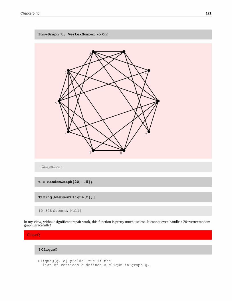
ShowGraph@t, VertexNumber -> OnD

1

23

4

5

6

7 8

9

10

� Graphics �

t = RandomGraph@20, .5D;Timing@MaximumClique@tD;D80.828 Second, Null<

In my view, without significant repair work, this function is pretty much useless. It cannot even handle a 20−vertex random graph, gracefully!

CliqueQ

? CliqueQ

CliqueQ@g, cD yields True if thelist of vertices c defines a clique in graph g.

Chapter5.nb 121

CliqueQ@CompleteGraph@12D, Range@12DDTrue

CliqueQ@CompleteGraph@12D, Range@5DDTrue

CliqueQ@RandomGraph@10, .5D, Range@5DDFalse

MinimumVertexCover

? MinimumVertexCover

MinimumVertexCover@gD finds the minimum vertex cover of graph g.

? Highlight

Highlight@g, pD displays g with elements in p highlighted. Thesecond argument p has the form 8s1, s2,...<, where the si’sare disjoint subsets of vertices and edges of g. The options,HighlightedVertexStyle, HighlightedEdgeStyle, HighlightedVertexColors,and HighlightedVertexStyle are used to determine the appearancof the highlighted elements of the graph. The default settingsof the style options are HighlightedVertexStyle->Disc@FatD andHighlightedEdgeStyle->Fat. The options HighlightedVertexColorsand HighlightedEdgeColors are both set to 8Black, Red, Blue,Green, Yellow, Purple, Brown, Orange, Olive, Pink, DeepPink,DarkGreen, Maroon, Navy<. The colors are chosen from the paletteof colors with color 1 used for s1, color 2 used for s2, andso on. If there are more parts than colors, then the colorsget used cyclically. The function permits all the options thatSetGraphOptions permits, for example, VertexColor, VertexStyle,EdgeColor, and EdgeStyle. These options can be used to controlthe appearance of the non-highlighted vertices and edges.

122 Chapter5.nb

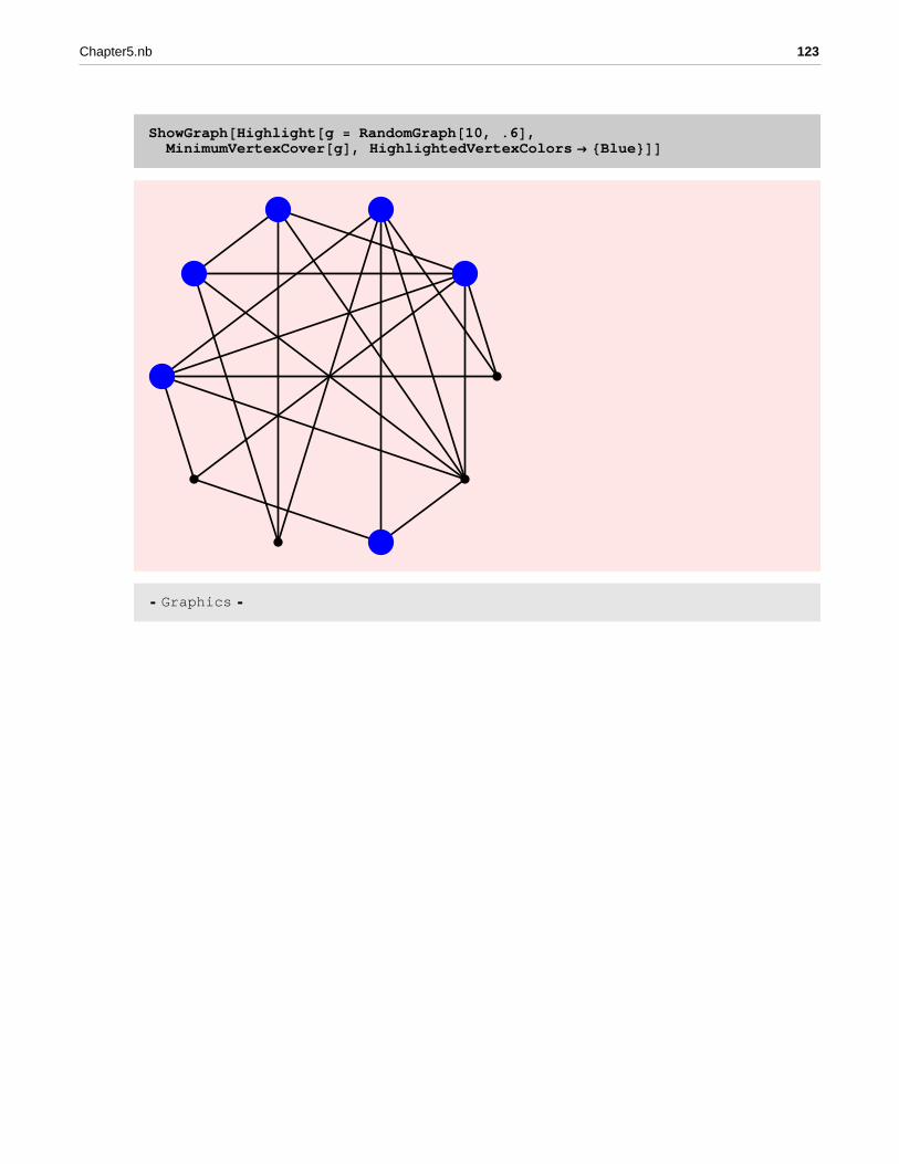
ShowGraph@Highlight@g = RandomGraph@10, .6D,MinimumVertexCover@gD, HighlightedVertexColors ® 8Blue<DD

� Graphics �

Chapter5.nb 123

ShowGraph@Highlight@g = RandomGraph@14, .3D,MinimumVertexCover@gD, HighlightedVertexColors -> 8Blue<DD

� Graphics �

VertexCoverQ

? VertexCoverQ

VertexCoverQ@g, cD yields True if thevertices in list c define a vertex cover of graph g.

MinimumVertexCover@GridGraph@4, 4DD$Aborted

c = 82, 4, 5, 7, 10, 12, 13, 15<82, 4, 5, 7, 10, 12, 13, 15<

124 Chapter5.nb

VertexCoverQ@GridGraph@4, 4D, cDTrue

VertexCoverQ@GridGraph@4, 4D, Complement@c, 82<DDFalse

MaximumIndependentSet

? MaximumIndependentSet

MaximumIndependentSet@gD finds the largest independent set of graph g.

ShowGraph@Highlight@g = RandomGraph@10, .4D,MaximumIndependentSet@gD, HighlightedVertexColors -> 8Purple<DD

� Graphics �

These algorithms for vertex cover, independent set, clique etc. are pretty useless. The need is for significant improvements in these algorithms, for simple and possibly randomized heuristics that provide good approximation etc.

Chapter5.nb 125

IndependentSetQ

? IndependentSetQ

IndependentSetQ@g, iD yields True if thevertices in list i define an independent set in graph g.

IndependentSetQ@CompleteGraph@3, 3D, 81, 2, 3<DTrue

IndependentSetQ@CompleteGraph@3, 3D, 83, 4<DFalse

PerfectQ

PerfectQ is definitely useless as it is. It cannot even compute whether a 8−vertex graph is Perfect or not. No point in having this function around.

126 Chapter5.nb