1

Christopher Monckton, Editor ♦ www.scienceandpublicpolicy.org

November 2010 | Volume 2 | Issue 11

SPPI Monthly CO2 Report

2

3

Global government is here. It will not go away easily. The authoritative Monthly CO2 Report for November 2010 explains what the Cancun climate summit really

achieved: the establishment of hundreds of interlocking bureaucracies, directed by a single shadowy Secretariat that

bids fair to become the unelected government of the world. Editorial Comment: Page 3.

Our graphs explained: An account of how we compile our authoritiative SPPI temperature and CO2 graphs. Page 4.

IPCC assumes CO2 concentration will reach 836 ppmv by 2100, but, on present trends, it will be well short. Pages 5-7.

Since 1980 global temperature has risen at only 2.9 °F (1.6 °C)/century, not 6 F° (3.4 C°) as IPCC predicts. Pages 8-11.

Sea level rose just 8 inches in the 20th

century, and has been rising since 1993 at a very modest 1 ft/century. Page 12.

Arctic sea-ice extent has been growing rapidly as usual following its summer minimum In the Antarctic, sea ice extent was

recently at its third-highest in the 30-year record. Global sea ice extent shows little trend for 30 years. Pages 13-17.

Hurricane and tropical-cyclone activity remains near its lowest since satellite measurement began. Pages 18-22.

Sunspot activity continues to underperform, following the long – and cool – solar minimum. Pages 23-24.

The (very few) benefits and the (very large) costs of the Waxman/Markey Bill are illustrated at Pages 25-28.

A Special Focus shows who is spending almost $1 bn to buy or bully public opinion on the climate. Page 29.

As always, there’s our “global warming” ready reckoner, the surest way to check policy costs against benefits. Pages 30-31.

And our selection of recent scientific papers of interest, compiled by Dr. Craig Idso of www.co2science.org. Pages 32-36.

The medieval warm period was real, global, and warmer than the present, as our global map shows. Page 37.

And finally ... in the weird world of taxpayer-funded climate science, bad news is good news! Page 38.

SPPI Monthly CO2 Report : : November 2010

Accurate, Authoritative Analysis for Today’s Policymakers

3

HE 16TH CONFERENCE of the Parties, said Ms. Christiana Figueres, its president, “is a litmus test of global-governance capacity”. There it was,

right out in the open. Yet the few commentators who pointed out that the Cancun agreement established several hundred new bureaucracies all over the world, all answerable to the shadowy but now immensely wealthy and powerful Secretariat of the States Parties to the UN Framework Convention on Climate Change, were pilloried by the Fascists of the “green” movement as mere world-government conspiracy theorists.

After Cancun, world government is a fact. It is here. It is real. It is costly. It is unelected. It is powerful. It will grow. It will be resented. It will be hated. But it will not easily be dislodged.

It is easy to establish a bureaucracy, provided that one has – as the Secretariat has – near-unlimited amounts of other people’s money to pay for it. But it is all but impossible to kill a bureaucracy once it has become established, except by revolution.

How will the world government develop? The EU, whose officials were present at Cancun in unbecomingly large numbers, is the role-model. Once a sufficient critical mass of taxpayers’ cash and governments’ consent has been won – and, at Cancun, the Secretariat won all that it had so long planned for, and more – the momentum of the panjandrum becomes unstoppable, like a snowball rolling down an endless slope, growing ever larger as it crushes everything in its wake.

To the long-suffering citizens of the West, the establishment of a lavishly-funded, atheistic-humanist, bureaucratic-centralist world government with real but carefully-unaccounted wealth and real but carefully-concealed powers has two principal consequences. First, it is and will continue to be expensive. Students rioting and attacking members of the Royal Family with sticks in London would realize, if they were capable of thought, that the money already paid out by their true-believing “green” government to Save The Planet is already more or less equal to the entire cost of their tuition and accommodation while in college. Were it not for the “global warming” nonsense, their fees could and would be met in full, as those of previous generations were.

Secondly, the advent of global government-by-stealth marks the craven political abdication of the West. In particular, it marks the end of democracy worldwide. No ordinary citizens will have any right whatsoever to elect by universal secret ballot those who will in future regulate them and tax them. Where now are the uppity Bostonians who, incensed by a modest British tax on their tea, poured it not into their teapots but into the harbor, precipitating the American revolution that brought true, radical democracy not only to the States of the Union but to many other nations whose peoples admired what the Founding Fathers had achieved?

Now, all but the appearance is gone. Congress will still be elected, but it will increasingly be subject to and answerable to the new world power. Few will notice at first: the media will not – will not – tell them. Monckton of Brenchley

T

Editorial : : Global Governance Is Here

Mainstream Media Missed the Real Significance of Cancun

4

Letting the real-world data speak out EFORE we began producing the Monthly CO2 Reports, it

was easy for “global warming” profiteers to pretend, and

repeatedly to state, that “global warming” is “getting worse”,

and that the climate is changing “faster than expected”. Now they

are unable to get away with such falsehoods as easily as before.

The centerpieces of our monthly series of graphs showing what is

happening in the real world are our CO2 and temperature graphs,

now regarded as the definitive standard worldwide.

Our CO2 concentration graphs show changes in real-world CO2

concentration as measured by monitoring stations worldwide and

compiled by NOAA. We also calculate and display the least-squares

linear-regression trend on the real-world data. Because this trend has

been very close to a straight line since late 2001, it is a better guide

to future CO2 concentration than the UN’s projections that we also

display, based on its A2 “business as usual” scenario – the one that

comes closest to reality at present. The one difference is that, for

clarity, we zero the UN’s projections to the start-point of the linear

regression trend on the real-world data.

The UN predicts that, this century, CO2 concentration will rise

exponentially – at an ever-increasing rate – towards 836 [730, 1020]

parts per million by volume in 2100. In reality, however, for ten

years CO2 concentration has been following an exponential curve

towards just 618 ppmv by 2100. If this trend continues, the UN’s

central estimate of CO2 concentration is excessive.

Our global-temperature graphs show changes in real-world

temperature at or near the Earth’s surface. Each temperature graph

represents the mean of two satellite datasets: the monthly lower-

troposphere anomalies from the satellites of Remote Sensing

Systems, Inc., and of the University of Alabama at Huntsville. We

do not use the Hadley/CRU or NCDC/GISS datasets: the Climate-

gate scandal has shown these to be unreliable.

On each graph, the anomalies are zeroed to the least element in the

dataset. For clarity, the IPCC’s range of predictions is zeroed to the

start-point of the least-squares linear-regression trend on the real-

world data. Since late 2001, global temperature has been falling.

To preserve consistency with the IPCC’s published formulae for

evaluating climate sensitivity to atmospheric CO2 enrichment, the

IPCC’s projections are evaluated directly from its projected

exponential growth in CO2 concentration using the IPCC’s own

logarithmic formula for equilibrium temperature change adjusted for

transient warming, yielding a net near-linear range of projections.

Equilibrium change – final temperature response when the climate

has settled down after an external perturbation – is greater than the

transient change predicted by the UN. However, on the A2 scenario

that we use, the difference by 2100 is just 0.5 C° (0.9 F°). Therefore,

when the UN and other scientists say that global warming “in the

pipeline” will go on for “thousands of years”, just 0.5 C° of

additional warming is all that they are talking about.

B

SPPI Monthly CO2 Report : : Our Graphs

Your Monthly Update On What Is Really Happening With The Climate

5

CO2 concentration rises, but not at the predicted ever-increasing rate

CO2 is rising in a near-straight line, well below the IPCC‟s projected range (pale blue region). The deseasonalized real-world data are shown as a thick, dark-blue line overlaid on the least-squares linear-regression trend, heading for 570 ppmv by 2100, compared with the 730 ppmv predicted by the IPCC. The rate of CO2 growth has been gently declining for more than a decade, and – on present trends – will not reach even the minimum 2100 value of 730 ppmv projected on the IPCC‟s A2 scenario. Data source: NOAA.

6

IPCC predicts rapid, exponential CO2 growth that is not occurring

Observed CO2 growth is near-linear, and is nothing like as steeply exponential as predicted by the UN‟s climate panel. If CO2 concentration does not rise as rapidly as the IPCC predicts, nor will temperature. Data source: NOAA.

7

Projecting the past decade‟s CO2 trend to 2100 cuts IPCC forecasts

The dark-blue line shows CO2’s actual path, well below the exponential-growth curves (bounding the pale blue region) predicted by the IPCC in its 2007 report. Note that our graphs use true exponential curves, not the supra-exponential curves of the IPCC (which nevertheless says its A2 projections for CO2 are exponential). If CO2 continues on its present path, the IPCC‟s central temperature projection for the year 2100 must be considerably reduced. Data source: NOAA.

8

The 30-year global warming trend is just 2.9 °F (1.6 °C) per century

Global temperature for the past 30 years has been undershooting the IPCC‟s currently-predicted warming rates (pink region). The warming trend (thick red line) has been rising at well below half of the IPCC‟s central estimate. The El Nino of 2010 has now ended, and temperatures have fallen back to the long-run trend-line. Data source: SPPI index, compiled as the arithmetic mean of the monthly global lower-troposphere temperature anomalies of Remote Sensing Systems Inc. and the University of Alabama at Huntsville. SPPI no longer uses any terrestrial-temperature datasets, because they have proven unreliable.

9

Hardly any „global warming‟ since the turn of the millennium

For almost a decade since the turn of the millennium on 1 January 2001, the trend in global temperatures has been small. The IPCC‟s predicted equilibrium warming path (pink region) bears no relation to the far lesser rate of “global warming” that has been observed in the 21st century to date. Note the very sharp peak in global temperature in early 2010, caused by a strong El Niño Southern Oscillation. Now that the El Niño has ended, it is unlikely that 2010 will set a new global instrumental-era temperature record. The previous record was set in the El Niño year of 1998. Source: SPPI global temperature index, the mean of the RSS and UAH datasets.

10

RSS satellite global temperature record since 1 January 2001

Remote Sensing Systems’ satellite record since the turn of the millennium on 1 January 2001 shows a minuscule warming trend in global temperatures over the present decade. Source: RSS Inc.

11

UAH satellite global temperature record since 1 January 2001

The University of Alabama at Huntsville’s recently-revised satellite record since the turn of the millennium on 1 January 2001 echoes the RSS dataset in showing a slight warming trend in global temperatures over the decade. However, this warming trend, at just 0.9 C° per century, is nothing like as high as the IPCC predicts. The contrast between the RSS and UAH graphs exemplifies data uncertainties. Source: UAH.

12

Sea level continues to rise more slowly than the UN predicts

Sea level (anomaly in millimetres) is rising at just 1 ft/century: The average rise in sea level over the past 10,000 years was 4 feet/century. During the 20th

century it was 8 inches. As recently as 2001, the IPCC had predicted that sea level might rise as much as 3 ft in the 21st century. However, this maximum was

cut by more than one-third to less than 2 feet in the IPCC’s 2007 report, with a central estimate of 1 ft 5 in. Mörner (2004) says sea level will rise about 8

inches in the 21st century. Mr. Justice Burton, in the UK High Court, bluntly commented on Al Gore’s predicted 20ft sea-level rise as follows: “The

Armageddon scenario that he depicts is not based on any scientific view.” A fortiori, James Hansen’s prediction of a 246ft sea-level rise, made in an article

in The Guardian in 2009 is mere rodomontade. Source: University of Colorado, 2010, release 5.

13

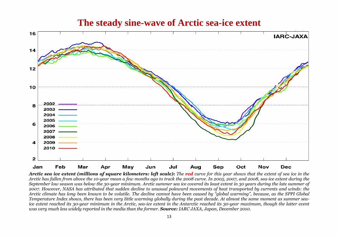
The steady sine-wave of Arctic sea-ice extent

Arctic sea ice extent (millions of square kilometers: left scale): The red curve for this year shows that the extent of sea ice in the Arctic has fallen from above the 10-year mean a few months ago to track the 2008 curve. In 2005, 2007, and 2008, sea-ice extent during the September low season was below the 30-year minimum. Arctic summer sea ice covered its least extent in 30 years during the late summer of 2007. However, NASA has attributed that sudden decline to unusual poleward movements of heat transported by currents and winds: the Arctic climate has long been known to be volatile. The decline cannot have been caused by “global warming”, because, as the SPPI Global Temperature Index shows, there has been very little warming globally during the past decade. At almost the same moment as summer sea-ice extent reached its 30-year minimum in the Arctic, sea-ice extent in the Antarctic reached its 30-year maximum, though the latter event was very much less widely reported in the media than the former. Source: IARC JAXA, Japan, December 2010.

14

... and the same graph from the Danish Meteorological Institute

Recovering to the mean: The Danish Meteorological Institute‟s graph of Arctic sea-ice extent (millions of square km on left scale: 2010 in black) shows Northern-Hemisphere sea ice returning to what has been normal in the past decade. Short-run fluctuations either side of the decadal mean are to be expected, and do not indicate long-run changes. Source: DanMet.

15

... and summer minimum sea-ice extent grew 24% in 2 years

Arctic summer sea-ice extent (purple) increased in 2008 and 2009, and in 2010 is similar to 2008, a little below the mean for the past decade, though well within natural variability. Since there has been little “global warming” since 1995, and since the decline in summer sea-ice extent has occurred only in the past five years, the decline that occurred in 2007 cannot be attributed to “global warming”. A paper by NASA in 2008 attributed the 2007 summer sea-ice minimum to unusual poleward winds and currents bringing warm weather up from the tropics. A few weeks after the Arctic sea-ice minimum, there extent of Antarctic sea ice reached a 30-year maximum. The Arctic was in fact 2-3 F° warmer in the 1930s and early 1940s than it is today.

A recent paper suggesting that the Arctic is now warmer than at any time for 2000 years is based on the same defective data, and is by the same authors, as the UN‟s attempt to abolish the medieval warm period in its 2001 report. In fact, for most of the past 10,000 years the world – and by implication the Arctic – was appreciably warmer than it is today. One of the authors of that report had previously told a fellow-researcher, “We have to abolish the medieval warm period.” However, papers by almost 800 scientists from more than 450 institutions in more than 40 countries over more than 20 years establish that the medieval warm period was real, was global, and was warmer than the present. Source: University of Illinois, 15 September 2009.

16

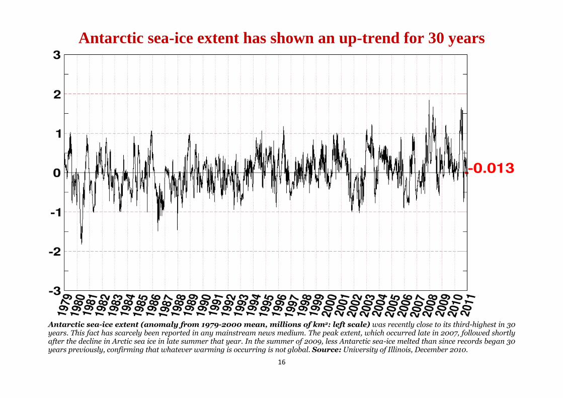
Antarctic sea-ice extent has shown an up-trend for 30 years

Antarctic sea-ice extent (anomaly from 1979-2000 mean, millions of km2: left scale) was recently close to its third-highest in 30 years. This fact has scarcely been reported in any mainstream news medium. The peak extent, which occurred late in 2007, followed shortly after the decline in Arctic sea ice in late summer that year. In the summer of 2009, less Antarctic sea-ice melted than since records began 30 years previously, confirming that whatever warming is occurring is not global. Source: University of Illinois, December 2010.

17

The regular “heartbeat” of global sea-ice extent: steady for 30 years

Planetary cardiogram showing global sea-ice area (millions of square kilometers: left scale): There has been a very slight decline in the trend (red) of global sea-ice extent over the decades, chiefly attributable to loss of sea ice in the Arctic during the summer, which was well below the mean in 2007, with some recovery in 2008 and a further recovery in 2009. However, the 2008 peak Arctic sea-ice extent was exactly on the 1979-2000 mean, and current sea-ice extent is not far below the 1979-2000 mean. The decline in summer sea-ice extent in the Arctic, reflected in the global sea-ice anomalies over most of the past decade, runs counter to the increase in Antarctic sea-ice extent over the period, suggesting that the cause of the regional sea-ice loss may not have been “global warming”. Source: University of Illinois, December 2010.

18

Hurricane, typhoon, and tropical-cyclone activity is at a 30-year low

Global and northern-hemisphere tr0pical-cyclone accumulated cyclone energy index, 1979-2010 (ACE units: 104 kts2): Global tropical-cyclone, typhoon, and hurricane activity remains close to its 30-year low. Since Hurricane Katrina (August 2005) and the publication of high-profile papers in Nature and Science, global tropical cyclone Accumulated Cyclone Energy has collapsed by half. This continues the now 5-consecutive-years‟ global crash in tropical cyclone activity. While the Atlantic on average makes up about 10% of the global, yearly hurricane activity, and the 2009 hurricane season in the North Atlantic was only half as active as normal, the other 90% of worldwide tropical-cyclone activity has also been significantly depressed since 2007.

The graph shows the 24-month running sum of tropical-cyclone energy from January 1979 for the entire globe (top) and the Northern Hemisphere only (bottom). The difference between the two time series is the Southern Hemisphere total. Intensity estimates of southern-hemisphere cyclones are often missing before the graph‟s start-date. Source: Ryan Maue, Florida State University, December 2010.

19

Combined tropical-storm and hurricane record: 40 years‟ decline

Combined frequency of tropical storms and hurricanes around the world and in each hemisphere (12-month running total of storms: left axis)

shows a small decline over the past 40 years of “global warming”. So far, there is little evidence in the hurricane record to suggest that warmer weather

produces more hurricanes. Source: Dr. Ryan Maue, Florida State University, December 2010.

20

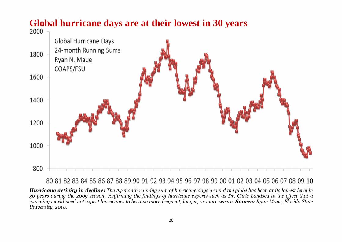
Global hurricane days are at their lowest in 30 years

Hurricane activity in decline: The 24-month running sum of hurricane days around the globe has been at its lowest level in 30 years during the 2009 season, confirming the findings of hurricane experts such as Dr. Chris Landsea to the effect that a warming world need not expect hurricanes to become more frequent, longer, or more severe. Source: Ryan Maue, Florida State University, 2010.

21

Global major hurricane days are almost at their lowest in 30 years

Extreme hurricanes are not common at present: The 24-month running sum of major hurricane days around the globe is not far above its lowest level in the 30-year record, confirming that mere warming of the planet does not necessarily entail more intense hurricanes. Source: Ryan Maue, Florida State University, 2010.

22

Almost no trend in North Atlantic hurricane activity for 60 years

North Atlantic Accumulated Cyclone Energy Index (ACE: left scale), 1950-2010: The ACE is a 24-month running sum that represents the combined frequency, intensity, and duration of hurricanes and tropical cyclones. Historically, the North Atlantic hurricane activity is usually characterized as a feast or a famine, making definitions of what is normal difficult. In "active" periods (such as 1995-present), a "normal" season sees much hurricane activity compared to inactive periods (such as 1970-1994). In the above figure, the light blue line indicates the linear trend of North Atlantic accumulated cyclone energy from 1950-2009 – a 60-year period of decent records – and the line is almost flat: no trend since 1950. When seasonal forecasters like Gray & Klotzbach at CSU and Tropical Storms Risk announce their upcoming seasonal forecast, they represent an entire season's worth of activity in an integrated sense either by predicting counts/frequency or ACE. However, there is no reason to assume that the entire hurricane season between June and November will experience uniform favorable or unfavorable atmospheric and oceanic conditions for tropical-cyclone formation. Indeed, the North Atlantic tends to spurt activity. For instance, one storm after another may form from African Easterly Waves and trek across the main development region for Atlantic hurricanes during the peak of the season. Source: Ryan Maue, Florida State University, 2010.

23

Solar activity is heading for what may be a small 2013 maximum

Monthly solar sunspot numbers (black curve, smoothed in blue, and predicted in red) since January 2000: Sunspot activity had been less than for 100 years, but is now recovering as the new solar cycle gets under way. However, the recovery of solar activity is behind the predicted curve. Note that the currently-predicted solar maximum for 2013-14 is considerably less intense than the previous solar maximum in 2000-01. However, the solar flux reaching the top of the atmosphere typically varies by only 0.15% between the minimum and the maximum of the ~11-year solar cycle. Source: ISES/NOAA/SWPC, Boulder, CO, USA, December 2010.

24

The minima of solar cycles 23 and 24 compared

Number of days without any visible sunspots during the previous solar minimum (blue) and the present solar minimum (red). During the last ~11-year solar minimum, in September/October 1996, the longest period without sunspots was 37 days, compared with 44 days in March/April 2009 and 51 days in July/August 2009. Source: Jan Alvestad, February 2010.

25

The stupefying cost of the Waxman/Markey Climate Bill

This postcard has all the key figures on the Waxman/Markey climate Bill in one place. Bottom line: to prevent the 3.4 C warming projected by the UN for this century under the A2 carbon emissions scenario would take 1360 years even if the Bill were fully implemented, and would cost $250 trillion. Source: SPPI calculations.

26

Why cap-and-trade will not change the global climate one iota

A pointless Bill: The Waxman/Markey Bill will cost billions to implement, but will reduce US carbon emissions hardly at all, unless the numerous exceptions in the Bill are implemented, in which event it will not reduce US carbon emissions at all. Source: www.breakthrough.org.

27

The Waxman/Markey Climate Bill will scarcely affect temperatures

Temperature change predicted by the UN, and (dotted line) adjusted to reflect the negligible impact of the Waxman/Markey Climate Bill, which might cut temperatures by 0.2-0.02 F by 2100, at a cost of $18 trillion. Source: Chip Knappenberger: cost estimates $180 bn/year from the White House.

28

The Waxman/Markey Climate Bill will scarcely affect sea level

Sea-level change predicted by the UN, and (dotted line) adjusted to reflect the negligible impact of the Waxman/Markey Climate Bill, which might cut sea-level by less than half an in by 2100, at a cost of $18 trillion. Source: Chip Knappenberger: cost estimates $180 bn/year from the White House.

29

Buying public opinion with tax-free dollars

„Global warming‟ is no longer a major concern with the public. Yet private foundations alone have contributed almost $1 billion to climate-extremist propaganda groups in the US alone in the past decade, as publicly-available tax filings reveal. And that is before one counts the vast taxpayer-funded public subsidies to climate propaganda groups.

Private buyers of public opinion on „global warming‟

William & Flora Hewlett Foundation $503,110,692 (2003 – 2010)

Pew Charitable Trusts $73,438,620 (1998 - 2006)

David & Lucile Packard Foundation $48,441,964 (1999 – 2009)

McKnight Foundation $48,025,000 (2008 – 2010)

Energy Foundation $38,500,495 (2003 - 2009)

Doris Duke Charitable Foundation $25,412,600 (2007 – 2009)

Who got most of the cash to buy public opinion

ClimateWorks Foundation $514,905,182 for 5 years’ support

Alliance for Climate Protection $27,750,000

Environmental Defense $25,268,538

Clean Air Task Force $4,917,635

Some individual beneficiaries

Gore Alliance for Climate Protection $114,000,000 (2006-9)

ClimateWorks $10,000,000 (2008)

Open Society Institute $5,000,000 (2008)

Richard and Rhoda Goldman Fund $7,500,000 (2007 – 2008)

The Lincy Foundation $15,000,000 (2008)

The Skoll Foundation $20,000,000 (2008 – 2009)

Silicon Valley Community Foundation $10,000,000 (2009)

The Benificus Foundation $10,000,000 (2008)

Grants made to the Energy Foundation alone

ClimateWorks: $31,100,000 (2008)

David & Lucile Packard Foundation $64,584,800 (2001-8)

Doris Duke Charitable Foundation $42,080,000 (2007-8)

John D. and Catherine T. MacArthur

Foundation $12,000,000 (2005)

MacArthur Foundation $17,000,000 (2005-6)

McKnight Foundation $51,429,780 (2001-10)

Mertz Gillmore Foundation $8,515,000 (2002-8)

SPPI Monthly CO2 Report : : Special Focus

Funds For Climate Extremism: Who Pays?

30

Your ‘global-warming’ ready reckoner Here is a step-by-step, do-it-yourself ready-reckoner which will let you use a pocket calculator to make your own

instant estimate of global temperature change in response to increases in atmospheric CO2 concentration.

STEP 1: Decide how far into the future you want your forecast to go, and estimate how much CO2 will be in the atmosphere at that date.

Example: Let us do a forecast to 2100. The Monthly CO2 Report charts show CO2 rising to C = 575 parts per million by the end

of the century, compared with B = 385 parts per million in late 2008.

STEP 2: Next, work out the proportionate increase C/B in CO2 concentration. In our example, C/B = 575/385 = 1.49.

STEP 3: Take the natural logarithm ln(C/B) of the proportionate increase. If you have a scientific calculator, find the natural logarithm

directly using the “ln” button. If not, look up the logarithm in the table below. In our example, ln 1.49 = 0.40.

n 1.05 1.10 1.15 1.20 1.25 1.30 1.35 1.40 1.45 1.50 1.55 1.60 1.65 1.70 1.75 1.80 1.85 1.90 1.95 2.00

ln 0.05 0.10 0.14 0.18 0.22 0.26 0.30 0.34 0.37 0.41 0.44 0.47 0.50 0.53 0.56 0.59 0.62 0.64 0.67 0.69

n 2.05 2.10 2.15 2.20 2.25 2.30 2.35 2.40 2.45 2.50 2.55 2.60 2.65 2.70 2.75 2.80 2.85 2.90 2.95 3.00

ln 0.72 0.74 0.77 0.79 0.81 0.83 0.85 0.88 0.90 0.92 0/94 0.96 0.97 0.99 1.01 1.03 1.05 1.06 1.08 1.10

STEP 4: Choose a climate sensitivity coefficient c from the table below –

Coefficient c ... SPPI minimum SPPI central SPPI maximum IPCC minimum IPCC central IPCC maximum

... for C° 0.7 1.4 2.1 2.9 4.7 6.5

... for F° 1.25 2.50 3.75 5.25 8.5 11.75

STEP 5: Find the temperature change ΔT by multiplying the natural logarithm of the proportionate increase in CO2 concentration by

your climate sensitivity coefficient. In our example we’ll choose the SPPI central estimate c = 2.50 F. Then –

ΔT = c ln(C/B) = 2.50 x 0.40 = 1.0 F°, your predicted manmade warming to 2100. It’s as simple as that!

SPPI Monthly CO2 Report : : Your Zone

How to calculate the effect of CO2 on temperature for yourself

31

Why cutting carbon emissions can never be cost-effective

A very simple calculation demonstrates definitively and conclusively that any attempt to address the imagined (and imaginary) “problem” of “global warming” is doomed not to be cost-effective. NOAA‟s global CO2 concentration record shows 388 parts per million by volume in the atmosphere in 2009/10. Throughout this millennium CO2 concentration has been rising in a straight line at 2ppmv/year, as our CO2 concentration graphs show every month. How much warming will this 2 ppmv/year increase cause? Using the formula for the UN‟s implicit central estimate of CO2‟s warming effect, taken from our Ready Reckoner, we can work this out thus: the warming, in Celsius degrees, is 4.7 times the Naperian logarithm of [(388+2)/388], which works out as 0.024 C° per year, or less than one-fortieth of a Celsius degree. So we should have to shut down the entire global carbon economy for 41 years, without any right to use an auto, train, or plane, to prevent just 1 Celsius degree of warming. However, the UN has exaggerated CO2‟s warming effect at least fourfold, so make that 160 years. Closing the entire carbon economy would in effect close the entire global economy. And all this for the sake of a non-solution to a non-problem.

32

fo

The Monthly CO2 Report summarizes key recent scientific papers, selected from those featured weekly at www.co2science.org,

that significantly add to our understanding of the climate question. This month we review papers about ocean acidification, sea

level rise, tropical cyclones and permafrost. Our final paper gives evidence that the Middle Ages were warmer than today.

Thirty-Second Summary

Larvae and juvenile sea stars raised at low pH grew and developed faster, with no negative effects on survival or skeletogenesis.

Reef islands may not disappear from atoll rims and other coral reefs in the near-future as speculated.

Empirical data suggest that tropical cyclone activity in the western hemisphere has grown slightly weaker as the earth has warmed

over the past six decades, which runs counter to climate-extremist claims.

Expansion of shrubs in the Arctic region, triggered by climate warming, may reduce summer permafrost thaw, and the increased

shrub growth may partially offset further permafrost degradation by future temperature increases.

Was there a Medieval Warm Period? YES, according to data published by 909 individual scientists from 540 separate research

institutions in 43 different countries in the CO2Science Medieval Warm Period Project database ... and counting! View an

interactive map here: http://www.co2science.org/data/timemap/mwpmap.html.

The fate of juvenile sea stars in an “acidified” ocean

Dupont, S., Lundve, B. and Thorndyke, M. 2010. Near future ocean acidification increases growth rate of the lecithotrophic larvae and juveniles of the sea star

Crossaster papposus. Journal of Experimental Zoology (Molecular and Developmental Evolution) 314B: 382-389.

According to Dupont et al. (2010), “Echinoderms are among the most abundant and ecologically successful groups of marine animals (Micael et

al., 2009), and are one of the key marine groups most likely to be impacted by predicted climate change events,” presumably because “the larvae

and/or adults of many species from this phylum form skeletal rods, plates, test, teeth, and spines from an amorphous calcite crystal precursor,

magnesium calcite, which is 30 times more soluble than normal calcite (Politi et al., 2004)”. This fact would normally be thought to make it

much more difficult for them (relative to most other calcifying organisms) to produce calcification-dependent body parts.

SPPI Monthly CO2 Report : : New Science

BREAKING NEWS IN THE JOURNALS, FROM www.co2science.org

33

Working with naturally-fertilized eggs of the common sea star Crossaster papposus, which they collected and transferred to five-liter culture

aquariums filled with filtered seawater (a third of which was replaced every four days), Dupont et al. tested this hypothesis by regulating the pH

of the tanks to values of either 8.1 or 7.7 by adjusting environmental CO2 levels to either 372 ppm or 930 ppm, during which time they

documented three results: settlement success as the percentage of initially free-swimming larvae that affixed themselves to the aquarium walls;

larval length at various intervals; and the degree of calcification achieved. The three researchers report that precisely the opposite of what is

often predicted actually happened. The echinoderm larvae and juveniles were “positively impacted by ocean acidification”. They found that

“larvae and juveniles raised at low pH grow and develop faster, with no negative effect on survival or skeletogenesis within the time-frame of

the experiment (38 days)”. The sea stars' growth rates were twice as high in the acidified seawater: “C. papposus seem to be not only more than

simply resistant to ocean acidification, but are also performing better.”

The Swedish scientists conclude that “in the future ocean, the direct impact of ocean acidification on growth and development potentially will

produce an increase in C. papposus reproductive success ... a decrease in developmental time will be associated with a shorter pelagic period

with a higher proportion of eggs reaching settlement”, leading the sea stars to become “better competitors in an unpredictable environment”. Not

bad ... especially for a creature that makes its skeletal rods, plates, test, teeth, and spines from a substance that is 30 times more soluble than

normal calcite.

References: Additional references from this review can be found at http://www.co2science.org/articles/V13/N34/B3.php.

The response of reef islands to warming-induced sea-level rise

Webb, A.P. and Kench, P.S. 2010. The dynamic response of reef islands to sea-level rise: Evidence from multi-decadal analysis of island change in the Central

Pacific. Global and Planetary Change 72: 234-246.

Webb and Kench report: “Under current scenarios of global climate-induced sea-level rise, it is widely anticipated that low-lying reef islands

will become physically unstable and be unable to support human populations over the coming century. It is also widely perceived that island

erosion will become so widespread that entire atoll nations will disappear, rendering their inhabitants among the first environmental refugees of

climate change.”

Members of the Maldives' Cabinet donned scuba gear in October 2009 and used hand signals to conduct business at an underwater meeting,

which was staged to highlight the imagined threat of global warming to the very existence of their country's nearly 1200 coral islands. At the

meeting, the cabinet signed a document calling on all nations of the Earth to reduce their carbon emissions, based on climate-extremist claims

that the greenhouse effect they say these emissions produce is raising temperatures, melting glacial and polar ice, and causing seawater to

expand and inundate low-lying islands.

34

In a study designed to explore the seriousness of this situation, Webb and Kench examined the morphological changes of 27 atoll islands in the

central Pacific in four atolls that span 15 degrees of latitude from Mokil atoll in the north (6°41.01' N) to Funafuti in the South (8°30.59' S) using

historical aerial photography and satellite images over periods ranging from 19 to 61 years. During that period, instrumental records indicated a

rate of sea-level rise of 2 mm/year in the central Pacific. The two researchers – one from Fiji and one from New Zealand – conclude: “There is

no evidence of large-scale reduction in island area despite the upward trend in sea level ... The islands have predominantly been persistent or

expanded in area on atoll rims for the past 20-60 years.”

Some 43% of the islands “increased in area by more than 3%, with the largest increases of 30% on Betio (Tarawa atoll) and 28.3% on Funamanu

(Funafuti atoll)”. The results of this study “contradict widespread perceptions that all reef islands are eroding in response to recent sea level rise

... Reef islands are geomorphically resilient landforms that thus far have predominantly remained stable or grown in area over the last 20-60

years. Given this positive trend, reef islands may not disappear from atoll rims and other coral reefs in the near-future as speculated.”

The ups and downs of tropical cyclone activity in the western hemisphere

Wang, C. and Lee, S.-K. 2009. Co-variability of tropical cyclones in the North Atlantic and the eastern North Pacific. Geophysical Research Letters 36:

10.1029/2009GL041469.

The authors write that in the western hemisphere tropical cyclones “can form and develop in both the tropical North Atlantic and eastern North

Pacific oceans, which are separated by the narrow landmass of Central America” ... in comparison with tropical cyclones in the North Atlantic,

those in the eastern North Pacific have received less attention, although tropical-cyclone activity is generally greater in the eastern North Pacific

than in the North Atlantic (e.g., Maloney and Hartmann, 2000; Romero-Vadillo et al., 2007)”. Exploring how the tropical-cyclone activities of

the North Atlantic and eastern North Pacfic ocean basins might be related to each other over the period 1949-2007, as well as over the shorter

period of 1979-2007, Wang and Lee used a number of different datasets to calculate the index of accumulated cyclone energy, which accounts

for the frequency, intensity and duration of all tropical cyclones in a given season.

The two US scientists discovered that “tropical-cyclone activity in the North Atlantic varies out-of-phase with that in the eastern North Pacific

on both interannual and multidecadal timescales ... When tropical-cyclone activity in the North Atlantic increases (decreases), tropical-cyclone

activity in the eastern North Pacific decreases (increases) ... the out-of-phase relationship seems to [have] become stronger in the recent

decades," as evidenced by the fact that the interannual and multidecadal correlations between the North Atlantic and eastern North Pacific

accumulated cyclone-energy indices were –0.70 and –0.43 respectively from 1949-2007, but –0.79 and –0.59 respectively from 1979-2007.

As for the combined tropical-cyclone activity over the North Atlantic and Eastern North Pacific ocean basins as a whole, there is little variability

on either interannual or multidecadal timescales. Real-world empirical data suggest that the variability that does exist over the two basins has

grown slightly weaker as the earth has warmed over the past six decades. This finding runs counter to climate-extremist claims that earth's

hurricanes or tropical cyclones should become more numerous, more intense and longer-lasting as temperatures rise.

References: Additional references from this review can be found at http://www.co2science.org/articles/V13/N44/C2.php.

35

Does warming reduce permafrost thaw rates?

Blok, D., Heijmans, M.M.P.D., Schaepman-Strub, G., Kononov, A.V., Maximov, T.C. and Berendse, F. Shrub expansion may reduce summer permafrost thaw in

Siberian tundra. Global Change Biology 16: 1296-1305.

The authors write that there are fears that if the Earth's permafrost thaws “much of the carbon stored will be released to the atmosphere”, as will

great quantities of the greenhouse gas methane (further exacerbating warming). Al Gore and other climate-extremists have claimed that this is

already happening at an accelerating rate. Michael Mann and Lee Kump (2008) in their Dire Predictions book make a similar claim.

Quite to the contrary, however, Blok et al. report that “it has been demonstrated that increases in air temperature sometimes lead to vegetation

changes that offset the effect of air warming on soil temperature”.

Blok et al. conducted a study in the Kytalyk nature reserve in the Indigirka lowlands of north-eastern Siberia, where they measured the thaw

depth or active-layer thickness of the soil, the ground heat flux, and the net radiation in 10-meter-diameter plots with and without a natural cover

of bog birch (Betula nana) shrubs.

Results indicated that “experimental B. nana removal had increased active-layer thickness significantly by an average of 9% at the end of the

2008 growing season, compared with the control plots”, which implies reduced warming in the more shrub-dominated plots, and that “in the

undisturbed control plots with varying natural B. nana cover, active-layer thickness decreased with increasing B. nana cover ... showing a

negative correlation between B. nana cover and active-layer thickness”, which again implies reduced warming in the more shrub-dominated

plots.

Blok et al. say their results suggest that “the expected expansion of deciduous shrubs in the Arctic region, triggered by climate warming, may

reduce summer permafrost thaw ... Increased shrub growth may thus partially offset further permafrost degradation by future temperature

increases.”

The six scientists add that permafrost temperature records “do not show a general warming trend during the last decade (Brown and

Romanovsky, 2008), despite large increases in surface air temperature”; that during the previous decade, “data from several Siberian Arctic

permafrost stations do not show a discernible trend between 1991 and 2000 (IPCC, 2007)”; and that “a recent discovery of ancient permafrost

that survived several warm geological periods suggests that vegetation cover may help protect permafrost from climate warming (Froese et al.,

2008)". They say this phenomenon “could feedback negatively to global warming, because the lower soil temperatures in summer would slow

down soil decomposition and thus the amount of carbon released to the atmosphere”.

References: Additional references from this review can be found at http://www.co2science.org/articles/V13/N42/C1.php.

36

The Middle Ages were warmer than today: Jinchuan peat marsh, Jilin Province, China

Hong, Y.T., Jiang, H.B., Liu, T.S., Zhou, L.P., Beer, J., Li, H.E., Leng, X.T., Hong, B. and Qin, X.G. 2000. Response of climate to solar forcing recorded in a 6000-

year δ18O time-series of Chinese peat cellulose. The Holocene 10: 1-7.

Working with cores extracted from a peat bog west of Jinchuan Town, Huinan County, Jilin Province, China (42°20'N, 126°22'E), the authors

developed “a 6000-year high-resolution δ18

O record of peat plant cellulose”, which they interpret as “reflecting changes in regional surface air

temperature”. Their results (see graph) show that the Medieval Warm Period, which was preceded by the Dark Ages Cold Period and followed

by the Little Ice Age, was considerably warmer than the current warm period.

37

Middle Ages: real, global, warmer than today

The Climategate emails reveal some of the tricks the IPCC‟s leading “scientists” used in an attempt falsely to abolish the Medieval Warm Period, so that they could pretend that today‟s temperatures are warmer than at any time in the past 1300 years. However, this graph from www.science-skeptical.de, a German website, shows graphs from scientific papers that examined proxy temperature data from all parts of the world. Visit the ScienceSkeptical.de website for an interactive version of the graph.

38

This Christmas card from Prof. Nils-Axel Mörner will be much appreciated by those of our northern-hemisphere readers who have endured exceptional snow this winter.