59

Spotlight on Modeling: Coupled Springs

Reference: Sections 3.1 and 6.4.In Chapter 3 we saw how to model the motion of a block attached to a single spring

under assumptions about the spring force and other forces acting on the block. Thatmodel involves a single second-order ODE that is equivalent to a normal first-ordersystem with the position and velocity of the block as state variables. The motions ofmultiple coupled springs and blocks also lead to a modeling system of normal first-order ODEs.

m1k2k1 m2

yx

Suppose that a coupled system of two blocks and two springs is attached to a wall,and the blocks slide back and forth on a smooth horizontal table (see the margin figure).At equilibrium, the springs are neither stretched nor compressed. Let’s measure therespective displacements of the blocks from their equilibrium positions by x and y,with the positive direction indicated by the arrows.

Suppose that air resistance and sliding friction are negligible, so the only forcesacting on each block are gravity, the upward force of the table, and the spring forces.Gravity and the upward force of the table are equal and opposite (Newton’s Third Law,Section 4.1), so we can ignore them. Suppose that each spring force is proportionalto the spring’s displacement from its equilibrium length (Hooke’s Law) and acts in adirection to restore the spring to its equilibrium length.

In particular, if the displacements of the blocks are x and y, then the spring forceacting on the block of mass m2 is −k2(y− x), where k2 is the positive Hooke’s Lawconstant for the spring. To check that the algebraic sign of the spring force is correct,observe that if y > x then the second spring is compressed and the spring force actsto decompress the spring. In this case the spring force on m2 should be directed to theright and should be negative (which it is). On the other hand, the spring connecting thetwo blocks exerts a force k2(y− x) on m1 that is equal and opposite in sign to the forceit exerts on m2 (Newton’s Third Law). Hooke’s Law implies that m1 is also subjectedto the spring force −k1x.

Apply Newton’s Second Law (Section 4.1) to each block:+ Use free-bodydiagrams to derive theseODEs. m1x′′ = −k1x+ k2(y− x) = −(k1+ k2)x+ k2 y

m2 y′′ = −k2(y− x) = k2x− k2 y(1)

System (1) models the vibration dynamics of the coupled spring-block configuration.Divide through by the masses to put system (1) in normal form. To make this nor-

malized second-order system acceptable to numerical solvers convert it to an equiva-lent normal first-order system.

EXAMPLE 1 The First-Order System that Models Coupled Springs/BlocksThe state variables for the coupled spring-block configuration modeled by system (1)are the position and velocity of each of the two blocks. Introduce new names x1, x2,x3, and x4 for the four state variables:

x1 = x, x2 = x′, x3 = y, x4 = y′

60

Then system (1) is equivalent to the undriven first-order linear system

x′1 = x′ = x2

x′2 = x′′ = −(

k1+ k2

m1

)x1+ k2

m1x3

x′3 = y′ = x4

x′4 = y′′ = k2

m2x1− k2

m2x3

(2)

System (2) is in normal form.

EXAMPLE 2 Linear System Notation for Coupled Springs and BlocksTake system (2) for a pair of coupled springs and blocks and specify some initialconditions. The corresponding IVP, x′ = Ax, x(0) = x0, is

x′ =

0 1 0 0

−k1+ k2

m10

k2

m10

0 0 0 1k2

m20 − k2

m20

x, x(0) = x0

The system matrix A is the 4× 4 constant matrix of coefficients given above.

Geometry of Solutions

Sometimes it is difficult to find solution formulas for differential systems that modelintricate natural processes. This is why the focus in this section is on qualitative prop-erties of solutions.

First, we review some notions about solutions of a system x′ = f (t, x), where xand f are n-vectors. A function vector x(t) defined on some t-interval I where t0 is asolution if x′(t) = f (t, x(t)) for all t in I. A solution of the system determines curveswhose behavior highlights properties of the solution.

v Curves Associated with Solutions. Suppose that x = x(t) is a solution ofthe system x′ = f (t, x). The point (t, x(t)) traces out a time-state curve in thetime-state space � n+1 of the variables t, x1, x2, . . . , xn. The projection of a time-state curve onto the tx j-plane is the x j- component curve. The projection of atime-state curve onto the x1, x2, · · · , xn state space is an orbit. A collection oforbits is an orbital portrait.

Let’s illustrate these concepts with graphs associated with the spring-block system.

EXAMPLE 3 Oscillating SpringsWhat happens if you compress the springs of Example 1 by pushing the first block one+ See the library

entries for Two LinearSprings under PhysicalModels.

61

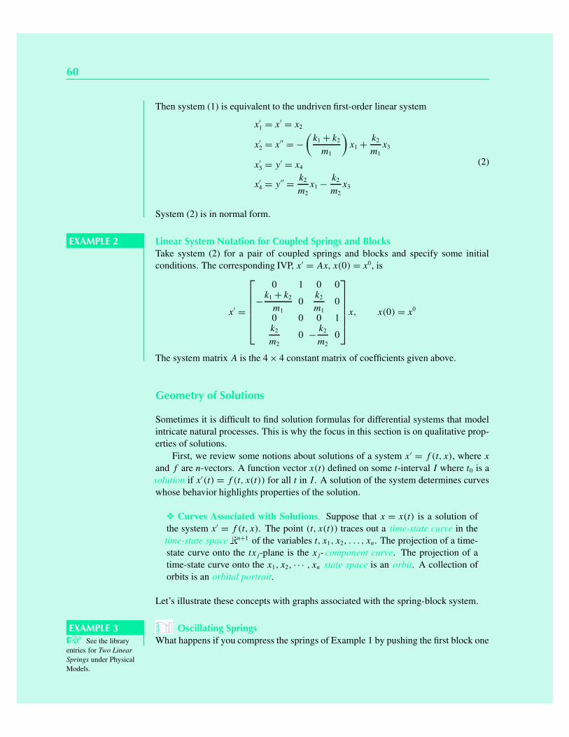
(1): x1(0)= 1, x2(0) = 0, x3(0)= 2, x4(0) = 0Po

sitio

nsx 1

,x3

ofbl

ocks

t

FIGURE 1 In-phase periodic oscillations of the cou-pled spring-block system (Example 3): first block(solid), second block (dashed).

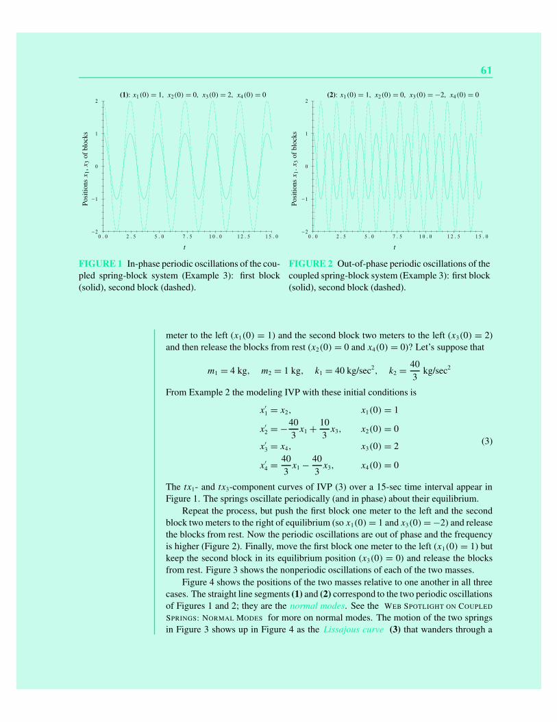
(2): x1(0)= 1, x2(0) = 0, x3(0)= −2, x4(0)= 0

Posi

tions

x 1.x

3of

bloc

ks

t

FIGURE 2 Out-of-phase periodic oscillations of thecoupled spring-block system (Example 3): first block(solid), second block (dashed).

meter to the left (x1(0) = 1) and the second block two meters to the left (x3(0) = 2)and then release the blocks from rest (x2(0) = 0 and x4(0) = 0)? Let’s suppose that

m1 = 4 kg, m2 = 1 kg, k1 = 40 kg/sec2, k2 = 403

kg/sec2

From Example 2 the modeling IVP with these initial conditions is

x′1 = x2, x1(0) = 1

x′2 = −403

x1 + 103

x3, x2(0) = 0

x′3 = x4, x3(0) = 2

x′4 =403

x1 − 403

x3, x4(0) = 0

(3)

The tx1- and tx3-component curves of IVP (3) over a 15-sec time interval appear inFigure 1. The springs oscillate periodically (and in phase) about their equilibrium.

Repeat the process, but push the first block one meter to the left and the secondblock two meters to the right of equilibrium (so x1(0)= 1 and x3(0)=−2) and releasethe blocks from rest. Now the periodic oscillations are out of phase and the frequencyis higher (Figure 2). Finally, move the first block one meter to the left (x1(0) = 1) butkeep the second block in its equilibrium position (x3(0) = 0) and release the blocksfrom rest. Figure 3 shows the nonperiodic oscillations of each of the two masses.

Figure 4 shows the positions of the two masses relative to one another in all threecases. The straight line segments (1) and (2) correspond to the two periodic oscillationsof Figures 1 and 2; they are the normal modes. See the WEB SPOTLIGHT ON COUPLED

SPRINGS: NORMAL MODES for more on normal modes. The motion of the two springsin Figure 3 shows up in Figure 4 as the Lissajous curve (3) that wanders through a

62

(3): x1(0) = 1, x2(0)= 0, x3(0) = 0, x4(0)= 0

Posi

tions

x 1,x

3of

bloc

ks

t

FIGURE 3 Both masses oscillate, but not periodi-cally (Example 3): first block (solid), second block(dashed).

(2)

(3)

(1)

(1): x1(0)= 1, x2(0) = 0, x3(0)= 2, x4(0)= 0(2): x1(0)= 1, x2(0) = 0, x3(0)= −2, x4(0)= 0(3): x1(0)= 1, x2(0) = 0, x3(0)= 0, x4(0)= 0

Posi

tion

x 3of

seco

ndbl

ock

Position x1 of first block

FIGURE 4 Periodic in-phase oscillations along line(1), out of phase along (2); nonperiodic along the Lis-sajous curve (3) (Example 3).

parallelogram.12

See the WEB SPOTLIGHT ON COUPLED SPRINGS: NORMAL MODES for actual solutionformulas. The spotlight also reveals why we used the initial data x1(0)= 1, x2(0)= 0,x3(0) = ±2, 0, x4(0) = 0.

We cannot show graphs of orbits or time-state curves for the model system ofExample 3 because we would need the four-dimensional x1x2x3x4-space for the formerat the five-dimensional tx1x2x3x4-space for the latter. However, the curves in Figure 1–4 are projections of these curves in four and five dimensional spaces into various planarspaces where we can see what happens.

The coupled spring system is linear, undriven and has constant coefficients, sothe methods of Section 6.4 apply. In particular, the eigenvalues of the matrix of co-efficients of the system in IVP (3) are ±i

√20 and ±i

√20/3, and the solutions in-

volve sinusoids of natural frequencies√

20 and√

20/3 (Problem 12). The graphs inFigures 1–4 strongly suggest sinusoidal solutions. The graphs also suggest that theamplitudes do not decay; that is because the system has no damping terms.

PROBLEMSHooke’s Law Spring (Review). The system x′ = y, y′ = −bx − ay+ A cosωt, a ≥ 0, b > 0, isequivalent to the scalar ODE x′′ + ax′ + bx = A cosωt that models the motion of a block attachedto a damped and driven Hooke’s Law spring. Find the solution x(t), y(t) of each IVP by using thetechniques of Chapter 3 to solve the equivalent scalar IVP.

12The 19th century French applied mathematician Jules Lissajous visualized the curves by reflecting light frommirrors on vibrating tuning forks onto a screen.

63

1. x′ = y, y′ = −x− y; x(0) = 1, y(0)= 0.

2. x′ = y, y′ = −x− 3y; x(0) = 1, y(0) = 0.

3. x′ = y, y′ = −25x+ cos 5t; x(0) = 0, y(0) = 0.

4. x′ = y, y′ = −25x+ cos(5.5t); x(0) = 0, y(0) = 0.�More Portraits of Orbits. Plot x- and y-component graphs, the orbit, and the time-state curve.Interpret what you see in terms of the behavior of the spring as t increases.

5. Problem 1, |x| ≤ 1, −0.75 ≤ y ≤ 0.25, 0 ≤ t ≤ 15.

6. Problem 2, 0 ≤ x ≤ 1, −0.3 ≤ y ≤ 0, 0 ≤ t ≤ 10.

7. Problem 3, |x| ≤ 1, |y| ≤ 5, 0 ≤ t ≤ 10. 8. Problem 4, |x| ≤ 2, |y| ≤ 2, 0 ≤ t ≤ 30.

Multiple Springs.

mk2k1

x 9. One Block and Two Springs Explain why the linear system, x′ = y, y′ = −(k1 + k2)(x/m)

models the undamped motion of the block-and-springs arrangement shown in the marginfigure. Then create a model with damping whose magnitude is proportional to velocity.

m1k2k1 m2

yx k3 10. Two Blocks and Three Springs (with Damping) Assume Hooke’s Law and damping propor-

tional to velocity; write a model system of two, second-order, linear, undriven ODEs for thesystem of springs and blocks shown in the margin figure. Then create an equivalent first-ordersystem. [Hint: look at Problem 9.]�

11. Two Blocks and Three Springs Set m1 = 4 kg, m2 = 1 kg, k1 = 40 kg/sec2, k2 = 40/3 kg/sec2,k3 = 20/3 kg/sec2 in the system that models the system of springs and blocks shown in themargin for Problem 10. Assume no damping and experiment with initial data and create pic-tures that resemble those shown in Figures 1–4. Then repeat, but with damping coefficientsc1 = c2 = 1 kg/sec. Interpret each graph in terms of the motions of the blocks.

12. Solution Formulas for Spring Systems Find the solution formula for the IVP (3). [Hint: usethe Method of Eigenvectors in Section 6.4 to solve the system.]

Sensitivity to Changes in the Data.�13. Coupled Hooke’s Law Springs: Response to Parameter Changes In system (2) take the

parameter values (k1 + k2)/m1 = 1, k2/m1 = α, k2/m2 = 1, where the magnitude of thepositive constant α is m2/m1. For these values, system (2) becomes

x′1 = x2, x′2 = −x1 + αx3, x′3 = x4, x′4 = x1 − x3

For each value of α = 0.05, 0.5, 0.95 plot� tx1- and tx3-component graphs for initial data (√α,0,1,0), and (−√α,0,1,0).� The projections onto x1x3x2-space of the orbit with initial data (2

√α,0,0,0).� The x1x3 Lissajous graphs for initial data (±√α,0,1,0) and (2

√α,0,0,0).

Use 0≤ t ≤ 25 and describe for each value of α how the spring system behaves for each of thethree sets of initial values. What happens to the frequency of the oscillations as α increasesfrom 0.05 to 0.95? What happens to the amplitude?