static.tti.tamu.edu sponsorip.a. aa."ncy' nome and addr,," ~~a~e department of...
TRANSCRIPT

TECHNICAL REPORT STANDARD TlTL E PAG E
1. Report No. 2. Government Acce .. ion No. 3. R"cipient' $ Calalog No.
FHWA/TXf84/26+233-2F ··~------.l...------·----·-~-------ic5.'RO::,,:::-:po::-:-;rl:-;:O\:"al;:-e--·--· -_ ..
4. T"I" and Subtitl"
AN HiPROVED BRIDGE SAFETY INDEX FOR NARROW BRIDGES
---_ .. -.<._--._---_. --_. __ ._---7. Author'.)
R. B. V. Gandhi and R. L. Lytton
9. Performin.,\! Organi lolion Nom" and Addre .. Texas Iransportation Institute Texas A&M University System College Station, Texas 77843
f-:--::---------:--:---;-~;-- --.-.----.--------~ 12. Sponsorip.a. Aa."ncy' Nome and Addr,,"
Texas ~~a~e Department of Highways Transportation
Transportation Planning Division P.O. Box 5051; Austin, Texas 78763
15. Supplementary Not".
and Public
Work done in cooperation with FHWA, DOT. Study Title: Priority Treatment of Narrow Bridges
16. Abstract
August 1983
Research Report 233-2F
! 10. Work Unit No.
11. Contract or Granl No.
Study 2-18-78-233 13. Type of Reporl and Period Covered
Final _ September 1977 August 1983
14. Sponsoring Agency Code
In this report, a new bridge safety index is developed based upon an extensive statistical study of accident data on 78 bridges. A total of 655 accidents were recorded at these bridges over the six-year period between 1974 and 1979. Cluster analysis showed that 26 of the bridges could be grouped into a "less-safe ll class and the remaining 52 bridges culstered into the Ilmore-safell group. Assigning a score of 0 to the less-safe group and 1 to the more-safa group, logistic regression analysis was used to develop an equation for the probability that a bridge is safe. The R2 of the equation is 0.53 and i.ncludes the following variables bridge wid~h, bridge length, ADT, vehicle speed, grade continuity, shoulder reduction, and traffic mix. A sensitivity analysis shows that bridge safety may be improved most by reducing vehicle speed and secondly by increasing the bridge width. Recommendations are made for the data that should be collected and the number of bridges that should be represented in future studies.
The Bridge Safety Index developed in this study i·s considerably better than all that have been proposed previously since it is based objectively upon accident rates and has a much better correlation with accident rates than any previously proposed Bridge Safety Index. Consistent use of this index in setting funding priorities for projects to improve bridge safety should result in a reduction of accident rates, property damage, injuries and fatalities at bridges.
17. Key Words
Narrow Bridges, Bridge Safety Index, Funding Priorities
lB. Oi stribution Statement
No Restricitions. This document is available to the public through the National Technical Information Service, Springfield Virginia 22161
19. Security Classif. (of this r"port) 20. Security ClassH. (of thi $ pagel 21. No. of Pages 22. Price
Unclassified Unclassified 146 Form DOT F 1100.1 18·69)


AN IMPROVED BRIDGE SAFETY INDEX
FOR NARROW BRIDGES
by
R. B. V. Gandhi R. L. Lytton
Research Report Number 233-2F
Priority Treatment of Narrow Bridges Study No. 2-18-78-233
conducted for the State Department of Highways
and Public Transportation
in cooperation with the U. S. Department of Transportation
Federal Highway Administration
by the
TEXAS TRANSPORTATION INSTITUTE Texas A&M University
College Station, Texas
August 1983


ABSTRACT
In this report, a new bridge safety index is developed
based upon an extensive statistical study of accident data
on 78 bridges. A total of 655 accidents were recorded at
these bridges over the six- year period between 1974 and
1979. Cluster analysis showed that 26 of the bridges could
be grouped into a "less-safe" class and the remaining 52
bridges clustered into the "more-safe" group. Assigning a
score of 0 to the less-safe group and 1 to the more-safe
group, logistic regression analysis was used to develop an
equation for the probability that a bridge is safe. The
R2 of the equation is 0.53 and includes the following
variables: bridge width, bridge length, ADT, vehicle speed,
grade continuity, shoulder reduction, and traffic mix. A
sensitivity analysis shows that bridge safety may be
improved most by reducing vehicle speed and secondly by
increasing the bridge width. Recommendations are made for
the data that should be collected and the number of bridges
that should be represented in future studies.
The Bridge Safety Index developed in this study is
considerably better than all that have been proposed
previously since it is based objectively upon accident rates
and has a much better correlation with accident rates than
any previously proposed Bridge Safety Index. Consistent use
ii

of this index in setting funding priorities for projects to
improve bridge safety should result in a reduction of
accident rates, property damage, injuries and fatalities at
bridges.
iii

SUMMARY
A Bridge Safety Index should be able to indicate
reliably which bridges are more likely to cause accidents
and what can be improved to reduce the accident rate at
those bridges. This report documents the development of an
objective bridge safety index using an extensive statistical
study of accident data on 78 bridges. A total of 655
accidents were recorded at these bridges over a six- year
period between 1974 and 1979. A statistical technique known
as cluster analysis showed that 26 of the bridges clustered
into a "less-safe" class and the remaining 52 bridges
clustered into the "more-sa "group.
The study then investigated a number of characteristics
of the bridge, the approach roadway geometrics, the traffic,
and the driving environment including signs, pavement
markings, and distractions to determine which of these
contributed to the assignment of a bridge into either the
"more-safe" or "less-safe" bridge class. A total of 20 such
characteristics were studied some of which must be rated
subjectively but tables, graphs, and nomographs are provided
for that purpose.
Assigning a score of 0 to the less-safe group and 1 to
the more-sa group, logistic regression analysis was used
to develop an equation for the probability that a bridge is
iv

safe. The final equation includes the following variables:
bridge width, bridge length, average daily traffic (ADT),
vehicle speed, the degree of continuity of the approach and
departure grade, the reduction of the shoulder width from
the approach roadway to the bridge, and the traffic mix,
which is primarily based upon the percent trucks in the
traffic stream. The new equation has a correlation
coefficient (R) with accident rate of 0.53 which is
considerably better than that of the Bridge Safety Index
developed by TTl and reported in NCHRP Report 203, "Safety
at Narrow Bridge Sites. 1I The latter equation only had a
correlation coefficient of 0.23. No perfect correlation is
expected since accidents also depend upon the driver, which
was not considered in this study.
A sensitivity analysis shows that bridge safety may be
improved most by reducing vehicle speed, secondly by
increasing bridge width, and thirdly by reducing the number
of trucks in the traffic stream.
It is considered possible to improve still more on the
Bridge Safety Index that is developed in this report if more
data are available. It is estimated that over 200 bridges
would be needed for that purpose. Recommendations are also
made on the additional data that should be collected in the
event that it is considered desirable to improve the Bridge
Safety Index of this report.
The Bridge Safety Index developed in this study is
v

considerably better than all that have been proposed
previously since it is based objectively upon accident rates
and has a much better correlation with accident rates than
any previously proposed Bridge Safety Index. Consistent use
of this index in setting funding priorities for projects to
improve bridge safety should result in a reduction of
accident rates, property damage, injuries and fatalities at
bridges.
vi

IMPLEMENTATION STATEMENT
The Bridge Sa ty Index presented in this report can be
used together with project cost to determine a benefit-cost
ratio for proposed bridge safety improvement projects.
Because this Bridge Safety Index is based objectively on
accident rate data, consistent use of this index by the
Texas State Department of Highways and Public Transportation
to set funding priorities for projects to improve bridge
safety should result in a reduction of accident rates,
property damage, injuries and fatalities at bridges.
DISCLAIMER
The contents of this report reflect the views of the
authors who are responsible for the facts and the accuracy
of the data presented within. This report does not
constitute a standard, a specification or regulation.
vii

TABLE OF CONTENTS
ABSTRACT ••••••••••••••••••••••••••••••••••••••••••••• ii
SUMMARY •••••••••••••••••••••••••••••••••••••••••••••• iv
IMPLEMENTATION STATEMENT AND DISCLAIMER •••••••••••••• vii
LIST OF TABLES....................................... xi
LI ST OF FIGURES...................................... xii
CHAPTER 1. Introduction ••••••••••••••••••••••••••••• 1
CHAPTER 2. Literature Review •••••••••••••••••••••••• 5
Defining a Narrow Bridge •••• :................... 5
Factors Which Affect Safety at Bridges.......... 6
Methods Employed to Improve Safety at Bridges... 12
Relating Accidents to Highway and Bridge Fea tures. . . . . . . . . . . . . . . . . . . . . . . . . . . . . . . . . . . . . . . . 17
Summary. • . • • . • . • . • • . . . • . . . . . . • . . . • . . . . • . . • • • • . • • 29
CHAPTER 3. Preliminary Analysis of Data ••••••••••••• 31
Correlation Analysis............................ 33
Multicollinearity Diagnostics-variance Inflation Factors (VIF)......................... 35
Variable Selection with R2 as Indicator......... 36
Factor Analysis................................. 38
Conclusions About Existing Data................. 39
CHAPTER 4. Collection of Additional Data and Analysis of the Total Data............... 40
Total Data...................................... 40
Additional Data Collected....................... 41
Testing Statistically for Effect of Type of Bridge....................................... 43
viii

TABLE OF CONTENTS (cont'd)
Testing Statistically for the Effect of Sidewalks.. . . .. . ... . . .... .. ... ... . ... . .. ... . .. .. 44
A Histogram of the Accident Rate................ 44
Cluster Analysis of the Data.................... 46
A Correlation Analysis.......................... 48
Multicollinearity Diagnostics for Total Data.... 51
Simple Linear Regression with Some of the Independent Variables........................... 52
Stepwise Regression of the Total Data........... 54
Regression Analysis Using the SAS R-Square Procedure. • • . • • • • • • • • • • • • • • • • • • • • • • • • • • • • • • • • • • • 57
Factor Analysis of the Total Data............... 59
Testing for Normality of the Variables.......... 61
Discriminant Analysis........................... 62
Logistic Regression............................. 64
Sensitivity Analysis of the Logistic Model...... 66
Sensitivity Index............................... 68
Discussion of Regression, Discriminant and Logistic Models with the Independent Variables Selected in the Final Model..................... 70
Comparison of Safety Index Obtained with the Previous Safety Indices......................... 71
CHAPTER 5. Summary, Conclusions, and Recommendations.......................... 73
Summary......................................... 73
Conclusions..................................... 75
Recommendations for Future Investigations....... 78
ix

TABLE OF CONTENTS (cont'd)
REFERENCES. • • • • • • • • • • • • • • • • • • • • • • • • • • • • • • • • • • • • • • • • • • 80
APPENDIX A. Regression and Correlation Analysis and Allied Concepts and Procedures...... 89
APPENDIX B. Factor Analysis ••••••••••••••••••••••••• 105
APPENDIX C. Cluster Analysis •••••••••••••••••••••••• 113
APPENDIX D. Discriminant Analysis ••••••••••••••••••• 116
APPENDIX E. Testing for Normality ••••••••••••••••••• 120
APPENDIX F. Logistic Regression ••••••••••••••••••••• 124
APPENDIX G. Lists of Bridge Data and Site Locations. 131
x

LIST OF TABLES
Table 1. Factors Use to Determine Bridge
Table 2.
Table 3.
Table 4.
Table 5.
Table 6.
Table 7.
Table 8.
Table 9.
Safety Index ............................... .
Evaluation of F12 .......................... .
Variance Inflation Factors ••••••••••••••••••
24
26
36
Factor Loadings for Bridge F-Data ••••••••••• 38
Some Items from BRINSAP Files of Texas •••••• 40
Analysis of Variance for Type of Bridge ••••• 43
Analysis of Variance for Sidewalks •••••••••• 44
Analysis of Variance for Cluster Groups ••••• 46
Identification (ID) Numbers of the Bridges in Less-Safe Group •••.•••••••••••••••••••••• 47
Table 10. Variance Inflation Factors (Total Data) ••••• 51
Table 11. Regression Coefficients in Simple Linear
Table 12.
Table 13.
Table 14.
Table 15.
Table 16.
Table 17.
Table 18.
Table 19.
Regress i on. • • • • • • • • • • • • • • • • • • • • • • • • • • • • • • • • • 53
Regression Coefficients of Stepwise ·Regress i on ••••••••••••••••••••••••.•••••••••
Steps of Stepwise Regression ••••••••••••••••
Factor Loadings for Total Data with Fll and F 12 .................................... .
Factor Loadings for Total Data with F20
.••••
Results of the Normality Tests ••••••••••••••
Logistic Regression Model of Bridge Safety ••
Sensitivity Analysis ••••••••••••••••••••••••
Data for Sensitivity Index •••••.••••••••••••
55
56
60
60
61
65
67
69
Tab 1 e 2 0 • Sen sit i v i ty I n de x • • • • • • • • • • • • • • • • • • • • • • • • • • • 6 9
Table 21. Correlation Coefficients ••••••••••••••••...• 71
xi

LIST OF FIGURES
Page
Figure 1. weighting of Bridge Width Factor (F l ) ••••••• 21
Figure 2. Nomogram Used to Determine Fll •••••••.•••••• 27
Figure 3. Matrix of Significant Correlations of F-factors of Tseng's data at ex = 0.10....... 34
Figure 4. A Histogram of the Accident Rate •••••••••••• 45
Figure 5. Matrix of significant correlations including F11 and F 12 ••••••••••••••••••••••• 49
Figure 6. Matrix of significant correlations including the variable F20 •••••••••••••••••• 50
xii


CHAPTER 1
INTRODUCTION
A bridge may require replacement or rehabilitation for
a variety of reasons including structural, geometric, and
functional obsolescence, all of which may contribute to a
reduction in safety for the driving public. Oglesby and
Hicks (!) state that on the Federal-aid highway system, of
the 240,000 bridges inventoried, there are about 9000
structurally obsolete and 31,000 functionally obsolete
bridges. Several articles have been written in professional
journals and news magazines discussing the gravity of this
problem. Engineering News Record (~) reported that one in
six U.S. highway bridges is deficient and tabulated the
percentage of deficient bridges in each state. Iowa led the
list with 39%. U.S. News reported in an article (2) that
weak bridges are a growing hazard on the highways. Several
articles appeared on highway hazards in the Better Roads
Journal (i, .?' ~). The latest Better Roads inventory
showed that there are nearly 90,000 substandard bridges in
the U.S. To bring even a fraction of the bridges up to the
modern design standards involves billions of dollars. Until
recently, no federal aid was available to rehabilitate all
of these deficient bridges. However, after the enactment of
the Surface Transportation Act of 1978, there was a dramatic
1

increase in
rehabilitation
1982, $4.2
funds for
programs
billion
highway bridge replacement and
(2) • For the fiscal years 1979 to
were authorized for bridge
rehabilitation. The Better Roads Journal (~, ~) also
reported on funding increases and rehabilitation programs
undertaken in different states.
The American Association of State Highway and
Transportation Officials (AASHTO) published several manuals
and documents to standardize the design and maintenance of
the highway system (l!, ll, ~). All of the new
highways and bridges are generally built to these modern
standards. Special committees of the AASHTO have dealt with
bridge safety and maintenance problems (!l, !!, 15).
Since the Highway Safety Act was passed by the u.S. Congress
in 1973, the u.S. Department of Transportation placed high
priority on highway and bridge safety. The National Highway
Safety Needs Study (!i, !2) laid emphasis on improved
guard rail design and bridge widening for improving safety
at bridges. They also initiated periodic bridge inventory
and appraisal programs in all states on a standardized basis
(18). The highway safety programs are evaluated
periodically and reported to Congress (~).
In addition to structurally unsound bridges, there are
several other bridges in the u.S. which are structurally
adequate but narrow in width compared to the approach
roadway width. Narrowing of the roadway on the bridge
2
creates a significant accident potential for the driving
public. These accidents result from the impact of vehicles
on bridge abutments, approach guard rails and bridge
railings and from collisions with oncoming vehicles due to
the narrowness of the bridge. Public awareness of the
narrow bridge problem escalated after two major accidents at
narrow bridges in New Mexico and Texas took a toll of 28
lives. These accidents resulted in a subcommittee hearing
(20) in the u.s. Congress from June 12 to 14, 1973, and
the narrow bridge problem attained nationwide attention.
A comprehensive analysis of safety at narrow bridges
has been an ongoing research activity of the Texas
Transportation Institute (~) and a Bridge Safety Index
(BSI) has been formulated to distinguish between "more safe"
and "less safe" bridges on the basis of several factors
related to the bridge and the approach roadway. The
research reported here is related to the improvement of the
BSI model for better classification of narrow bridges.
Additional data were collected on factors which affect
safety, and analysis using modern statistical techniques
such as cluster, discriminant and factor analysis and
multivariate regression were used.
The procedure that was followed in developing a Bridge
Safety Index required seven basic steps:
1. Review the literature on bridge safety and determine
what other studies have shown to be significant
3

contributing factors to enhance bridge safety.
2. Examine and make critical analysis of the readily
available information as tabulated at the Texas
Transportation Institute (TTl) with a view to selecting
relevant and important variables to be included in the
Bridge Safety Index (BSI) model;
3. Collect additional data on bridge geometrics and
accidents to improve the existing BSI model;
4. Analyze the final data set to ascertain the potential
relationships between variables;
5. Develop an enhanced safety model to classify narrow
bridges as "more safe" or "less safe" when certain
bridge geometrics and conditions are known. The model
should be developed as objectively as possible using
variables that contribute significantly to accident
rate and those that can be readily improved to increase
bridge safety;
6. Obtain a Bridge Safety Index from the model that can be
used to identify a potentially hazardous narrow bridge;
7. Develop a methodology that can be used in general for
obtaining safety models for other types of bridges, as
well as other roadside structures that effectively
narrow the roadway.
The consistent use of the Bridge Safety Index in
helping to set priorities for
safety should reduce accident
projects to improve bridge
rates, minimize property
damage and human injury, and save lives.
4

CHAPTER 2
LITERATURE REVIEW
A significant amount of research has been conducted in
the united States on highway related accidents with a view
to improve public safety on the highway system. Although
the United States has one of the best highway systems in the
world, some bottlenecks still exist in the form of narrow
bridges, which pose a danger to high speed traffic. The
literature review presented here relates to the safety
problems at narrow bridges and what is being done to solve
them.
Defining a Narrow Bridge
A survey of narrow bridges (~) conducted by the
Texas Transportation Institute (TTl) showed that dif rent
States had different criteria for defining narrow bridges.
The questionnaire summary indicates that a large number of
state bridges, 7,211 in number, are considered narrow if
they are 18 feet or less in width, and a large number of
city and municipal bridges, 7,905 in number, are considered
deficient if they are 16 feet or less. TTl drew the
following conclusions from the survey:
1. The lower limit for two-way operations generally
appears to fall in the range of 16 to 20 feet.
5

2. In general, a bridge is considered narrow if the
clear roadway width on the bridge is equal to or
less than the approach roadway width.
Southwest Research Institute of San Antonio (SWRI) in
its study on narrow bridges (~) defined narrow bridges as
follows:
1. One-lane, 18 feet or less in width,
2. Two-lane, 24 feet or less in width,
3. Total approach width greater than total bridge
width (curb to curb) and bridge shoulder is less
than 50% of approach roadway shoulder (i.e., >50%
shoulder reduction).
According to Johnson (~),
driver's behavjor with regard
any bridge
to speed
that
or
changes
lateral
positioning of the vehicle can be considered "narrow". He
developed equations to estimate driver behavior in terms of
bridge perceptual parameters such as bridge width, length
and initial speed.
In general, it appears that anything less than a 24-
foot clear bridge width for a two-way bridge operation or a
reduction of the shoulder on the bridge or any factor that
causes changes in a driver's lateral position and speed
defines a "narrow bridge condition".
Factors Which Affect Safety at Bridges
Bridges pose a high accident potential especially when
6

the roadway is narrowed on the bridge. Common types of
accidents are collisions with guard rails on approach
roadways or collisions with bridge railings. If the bridge
width is narrow, drivers have a tendency to move in closer
to the centerline to draw safely away from the bridge
railing, but instead risk a collision with oncoming cars.
Several investigators have carefully studied these accidents
and suggested remedial measures.
Hilton (~) conducted an extensive study of bridge
accidents in Virginia and found that several geometric
characteristics predominate at the accident sites. Some of
the salient characteristics found were pavement transitions
at bridge approaches, approach roadway curvature to the
left, narrow bridge roadway widths, intersections adjacent
to bridges and combinations of these and other geometric
factors. He also found that the severity index (a ratio of
the proportion of persons killed to the proportion of all
accidents on the highway system in Virginia) was high for
the bridge accidents on interstate highways.
Gunnerson (~) studied 72 bridges in Iowa over a 12-
year period and found 65 bridges had a width of less than 24
feet which was the approach roadway width. Others had a 30-
foot width which was actually 6 feet wider than the approach
roadway width. He concluded that if the approach roadway is
widened but the bridge is not, there is an increase in the
accident rate, whereas on control bridges, where the bridge
is also widened, the accident rate decreases.
7

Raff (~) conducted an extensive study of accident
data from 15 states on rural highways covering 5000 miles.
The routes were grouped into a large number of short,
sections homogeneous
compared.
Some of
The study
the factors
and accident rates of the groups were
included both highways and bridges.
included in the study were number of
lanes, average daily traffic, degree of curvature, pavement
and shoulder widths and sight distance. Traffic volume was
found' to have a strong effect on accident rates on most
highway sections except at two-lane curves and
intersections. At bridges and underpasses there was found
to be great value in increasing the roadway width several
feet over the approach roadway.
Shelby and Tutt (~) evaluated the effect of two-lane
bridge widths on the lateral placement of vehicles. Lateral
placement of vehicles was measured at several bridge sites
both on the road and the approach roadway. The sites
included lane widths in the range of 11 to 19 feet. It was
established that bridge width has a definite influence on
the lateral placement of vehicles. Although the conclusions
were not definitive, it appeared that an average driver
needs a bridge lane width of about 20 feet in order to cross
the bridge with little or no deviation in lateral position
from that on the approach roadway.
Brown and Foster (~) conducted an investigation of
bridge accidents on rural highways in New Zealand. The
8

variables considered were: day and night; horizontal
alignment of approaches (straight approach, left curved
approach and right curved approach); place of impact (within
the bridge or several points in the approaches); and width
of bridge or approaches.
The researchers found that night time accidents are
more frequent than day time ones and recommended
reflectorization techniques for night visibility. They also
found that 60 percent of bridge accidents occurred within
the left hand approach, 20 percent occurred within the right
hand approach and the remaining took place within the bridge
structure. Furthermore, 70 percent of the bridge accidents
took place where the bridge width was less than 79% of the
approach roadway. The researchers recommended properly
designed guard rails to "deflect the vehicles back on to the
highway and/or away from the end posts."
As early as 1941, Walker (~) studied bridge width
and its influence on transverse positioning of vehicles on
the bridge. On the basis of transverse positioning of
freely moving vehicles on the bridges, he found that an
l8-foot pavement with 3-foot shoulders or a total roadway
width of 24 feet, requires a concrete bridge width of 26 to
28 feet in order to make the driver feel secure. The
greatest width of a bridge required for a 22-foot pavement
was found to be 30.6 feet. Sidewalks apparently added
nothing to the effective roadway width on the bridge because
9

transverse position occurred at a fixed distance from the
curb or from a parapet if there was no curb.
King and Plummer (l!) evaluated the lateral vehicle
placement on a simulated bridge of variable width and
concluded that there should be a minimum shoulder width of 4
to 6 feet on the bridge for safe traffic operations.
Taragin and Eckhardt (ll) determined from their study that
the shoulders on highways should be at least 4 feet wide to
provide maximum lateral clearance between vehicles . travelling in opposite directions. They suggested further
research on the effect of shoulder types and widths on
accident rates. In a further study, Taragin (~) found
that a relationship exists between vehicle speeds and
lateral positions of vehicles on highways with paved
shoulders.
Huelke and Gikas (ll) considered non-intersectional
fatalities a problem in roadway design. Sixty percent of
the accidents were single car, off-road collisions with
fixed objects such as trees, utility poles, bridge abutments
and guard rails.
Roberts (l!) studied the effect of bridge shoulder
widths with curbs on the operational characteristics of
vehicles. No strong relationship was observed between
bridge shoulder widths and accidents. Vehicles moved farther
away from the edge under all curbing conditions. There was
strong evidence that outside shoulders 6 feet wide would not
10

seriously affect the operational characteristics of vehicles
on bridges.
A computerized
roadside obstacles
Michigan (35)
inventory and priority analysis for
was carried out by Cunard and others in
They observed that 26% of all fatal
accidents in Michigan during the study
trees,
year involved
guard rails, collisions with fixed objects such as
etc. They recommended a priority-ranking system of roadside
obstacles based on the severity index of injuries caused for
improving the roadside environment.
Presence of bumps at the approach and exit ends of
bridges produce a traffic hazard. Hopkins and Deen (li)
studied this problem and stated that this was due to the
settlement of
built. They
consolidation
embankments on
suggested that
of soils should
preventive measures could
which approach roadways are
a careful analysis of
be made in advance so that
be taken. Bridge deck
deterioration is another problem which can create hazardous
conditions on the bridge. Several investigators studied
this problem and suggested methods of repair and the effects
of traffic vibrations during repairs (ll, ~).
An article in the Indian Concrete journal (39) deals
with methods of inspection and maintenance of highway
bridges using suitable equipment. The authors suggested a
periodic and systematic in-depth inspection of all bridges
in a planned way and prompt remedial action to be taken in
case defects are found.
11
Methods Employed to Improve Safety at Bridges
Highway engineers have been improving their designs and
taking preventive measures to increase safety at bridge
sites. These efforts have resulted, among other things, in
increased widths for new bridges, better geometric features
to guide the drivers safely through the bridge, improved
guard rails to deflect the cars safely from the barriers,
improved signs, markings and use of proper lighting or
reflective markers. Some of these developments are
discussed in detail in this section.
As early as 1947, the chief of the Bridge Division of
Public Roads Administration, Washington, D.C. described the
bridge design to significant changes occurring
improve safety (i!) • Some
were extending the full width
in
of
of
modern
the improvements mentioned
the roadway on to the
bridge, wider curbs and streamlined railings. Godwin (±!)
described how old wooden bridges in California are replaced
by small concrete slab culverts or pipe-arch installations.
A bridge parapet for safety was developed at General Motors
Proving Ground
concrete parapet.
the design met
(~) which consists of a tube railing on a
Tests at the proving ground showed that
many safety requirements, although it was
somewhat more expensive.
Zuk et.al. (~) , described various methods of
modifying historic bridges in Virginia for contemporary use.
Many of these old bridges were narrow and had low load
12

carrying capacities, making them targets for replacement.
On a case by case basis, the bridges were investigated for
their potential for strengthening and widening. Some were
explored for non-vehicular uses such as museums for historic
preservation.
In the article "New Highway Bridge Dimensions for
Safety", Clary (44) emphasized that safety must be the
first priority in design followed by cost, durability and
aesthetics. He suggested that maximum clearances must be
provided between a roadway and the exposed parts of bridges
such as piers and abutments. Bridge railings must be of
adequate strength and continuous with approach guard rails.
There must be adequate transition between the rigid bridge
railing and the flexible approach guard rail. Any
obstruction such as wide curb which might cause vaulting if
struck by a vehicle must be removed as far as practicable.
Openings between twin bridges must be eliminated where
feasible or they must be adequately protected by a guard
rail.
Under the sponsorship of the National Cooperative
Highway Research Program (NCHRP) considerable research was
conducted for improved designs of guard rails and bridge
rails to reduce severity of accidents. The main objective
was to deflect the vehicle away from the fixed object with
minimum impact, thus
reports (~, ~, il,
reducing accident severity. Several
~) were issued by the NCHRP on
13

guard rail design and evaluation which indicate considerable
progress in the development of safe guard rails. Under the
same program Olson and others (~, 50) developed design
criteria and guide lines for bridge rail systems.
Michie and Bronstad (~) gave guide lines for
location, selection and maintenance of traffic barriers.
They classified traffic barriers into two types: (1)
longitudinal systems (guard rails, bridge rails and median
barriers) and (2) crash cushion systems (to prevent head on
impact with fixed objects near bridges and off-ramp areas).
Examples of crash cushions include steel barrel
configurations, entrapment nets
filled with sand or water. They
and an array of containers
suggested that accidents
frequently may actually increase if these traffic barriers
are not properly selected and placed.
Nordlin et.al. (~), reported on five full scale
vehicle impact tests on California Type 20 bridge rail.
They found that the rail will retain and redirect a 4900 lb.
passenger car impacting at speeds up to 65 mph and approach
angles up to 25 degrees, with little or no damage to the
rail. Occupant
to moderate with
injuries varied from minor with seat belt,
no seat belt. Other researchers (53,
54) also reported on energy absorbing guard rails to
improve safety of the drivers. Post et • al • (55) ,
discussed the cost-effectiveness of two types of guard
rail-bridge rail transition improvements. The findings
14

showed that a double W-beam type used in Nebraska was
slightly superior to the AASHTO stiff post system.
Hunter et.al. (1!), gave methodology for ranking
roadside hazard correction programs. Initial runs on the
system indicated that use of transition guard rails at
bridge ends and tree removal at certain locations in North
Carolina were promising. A study undertaken in Texas (57)
showed that there are ways other than widening to improve
safety at narrow bridges. Good results were reported by
blending the approach rail smoothly with the bridge rail and
by using pavement markings to guide the driver on to the
narrow bridge.
The Texas Transportation Institute (~) suggested
fourteen alternative treatments to improve safety at narrow
bridges and indicated how these could be used in various
situations. Some of the fourteen treatments suggested are
changing approach grades, realigning the roadway, installing
smooth bridge rails and guard rails, placing edge lines,
installing narrow bridge signs, and advisory speed signs.
Three NCHRP reports (~, 59, 60) give methods for
evaluating highway safety improvements and determining the
cost-effectiveness of the programs. Rehabilitation and
replacement of bridges on secondary highways and local roads
were discussed in two recent reports which were also
published by the NCHRP (~, ~). Several types of
repair and rehabilitation procedures for correcting common
15

structural and functional deficiencies in highway bridges
and bridge decks were included in the two reports. Another
report of the NCHRP (~) gives guidelines for bridge
approach design to eliminate rough riding characteristics at
approaches to bridges.
Tamburri (~) and others discussed the effectiveness
of minor improvements in reducing accident rates. The
improvements included warning flashing beacons, safety
lighting installations in reducing night accidents,
protective guard rails and various delineation devices.
Protective guard rails were found to be very effective at
narrow bridges. The New Jersey State Highway Department
(~) found that low level lighting produced by fluorescent
lights mounted on bridge railings was very effective. An
article in Better Roads (~) considers the Danish practice
of wide edge and center line pavement markings using
thermoplastic materials as outstanding. Beaton and Rooney
(~) studied raised reflective markers for lane
delineation. They found fully beaded button markers more
effective than wedge markers in rainy weather at night on
concrete roads. They found wedge markers more durable on
asphalt roads than the button type. Turner and others
(~) found that full width paved shoulders reduce accident
rates on rural highways and especially on two lane roads.
The Manual on Uniform Traffic Control Devices (~)
describes standard signs for posting "NARROW BRIDGE" for two
16

way bridges with widths 16 to 18 feet and "ONE LANE BRIDGE"
if the bridge width is less than 16 feet for light traffic
or less than 18 feet for heavy commercial traffic.
Additional signs such as "NO PASSING ZONE", "YIELD", etc.
for advance warning of dangerous structures are also
sometimes recommended. A dynamic sign system (traffic
actuated) to alert motorists to the presence of narrow
bridges at an experimental main facility did not show much
difference between dynamic and normal
speed and lateral placement (2!).
signing in terms of
The role of signs in a
highway information system as well as several aspects in the
design were analyzed in detail in an NCHRP report (ll).
Relating Accidents to Highway and Bridge Features
To initiate corrective treatments for improving safety
at bridges, it is important to know which factors contribute
to the accident potential at bridges. Several researchers
attempted to relate roadway and bridge characteristics with
accident rates but achieved only a limited success because
of the complexity of the problem. Highway accidents involve
three principal elements: the driver, the vehicle, and the
highway. Highway features are only a part of the cause of
accidents. Driver behavior also plays an important part. A
major reason for the limited success of previous studies to
relate bridge and roadway characteristics to accident rates
is the non-uniformity in reporting and collecting accident
17

data. This is especially so of data collected in the past.
One of the earliest studies of bridge accidents was
conducted by Raff (~) for the Bureau of Public Roads in
1954. Accident data were collected from 15 states on
different types of road sections covering curves, straight
portions (tangents), structures, railroad crossings and
different grades (slopes). He first encountered the problem
of combining detailed data from different states but he
tried three different approaches to combine the data and
obtained three types of accident rates. His analysis showed
that traffic volume was found to have major effect on
accident rates. For roads carrying the same amount of
traffic, sharp curves had higher accident rates than flat
curves. Extra width in relation to the approach pavement
definitely reduced accident hazard on bridges.
Behnam and Laguros (~) attempted to relate accidents
at bridges to roadway geometrics at bridge approaches. They
studied eleven independent variables, some of which are
average daily traffic volume, bridge width, width of
approaching pavement, sight distance, curveline, height of
bridge rail, length of the bridge and travelling speed. For
the purpose of studying conditions in the driving
environment, the data were classified into several
categories including two-lane and four-lane rural highways.
Multivariate regression and stepwise regression procedures
were used in developing models. The models indicated that
18

average daily traffic (ADT) was one of the
variables and that the relationship
most significant
between traffic
accidents and geometric elements of a roadway are not linear
but can be expressed by a logarithmic transformation. On
two lane roadways sight distance (the greatest distance that
a driver can clearly see ahead while driving on the highway
in order to spot an obstacle on the road) was found to be
important for night driving, while the degree of curvature
became critical during day time.
Kihlberg and Tharp (73) conducted a study to relate
accident and severity rates for various highway types and to
various geometric elements of the highway. For the
statistical analysis of the data, the highway segments were
arranged into 15 ADT groups. The presence of geometric
elements (curves, grades, intersections and structures)
increased the accident rate on highways. The presence of
combinations of geometric elements generated higher accident
rates than the presence of individual
curvature affected accident rates
from zero value to 4 percent value.
did not affect the severity rates.
elements. Grade and
only when they changed
The geometric elements
Turner (~), using bridge accident data from Texas
and Alabama developed a probability table which predicts the
number of accidents per million vehicles for various
combinations of roadway width and bridge relative width.
His statistical investigation did not uncover a unique
19

combination of variables to predict accident rates
conclusively at specific structures. He attributed this to
the effects of minor variables not included in the bridge
data and to the fact that bridge accidents are complex with
multiple contributing aspects. He also developed a cost
effectiveness methodology for the relative evaluation of
various bridge safety treatments.
A comprehensive analysis of
narrow bridges was conducted by
safety specifically at
TTl for the NCHRP (21).
They identified ten important factors related to approach
roadway, bridge geometry, traffic and roadside distractions.
They developed a linear model combining these factors and
called it the Bridge Safety Index. The Bridge Safety Index
(BSI) could be expressed as:
BSI = Fl + F2 + F3 + ••••• + FIG
where
FI is a function of clear bridge width determined by
entering Figure 1 with the clear bridge width.
F2 is the ratio of the bridge width to the approach
roadway width, a measure of the relative
constriction of lateral movement as a vehicle
travels from the approach lane on to the bridge.
F3 is the approach guard rail and bridge rail
structural factor and attempts to define the safety
aspects of the rail and the contribution to bridge
perspective that the approach rail offers to an
20

,
20~----~------~------~--~--~
r-I 15 fi.! ..
H 0 .jJ u ctj
fi.!
.c: 10 .jJ "0 -..-I :s: w b'1 "0 -..-I
5 H lXl
o~--~~~--------~------~------~ 12 16 20 24 28
Bridge Width (Ft)
Figure 1. Weighting of Bridge Width Factor (F1)'
21

oncoming driver.
F4 is the ratio of approach sight distance (ft) to 85%
approach speed (mph) and indicates the time within
which a driver may prepare for the bridge crossing.
F5 is a measure of the approach curvature and is equal
to 100 + tangent distance to the curve
(ft)/curvature (degrees).
F6 is grade continuity (%) and denotes the average
grade throughout the bridge zone and the algebraic
difference in approach and departing grades.
F7 is shoulder reduction (%) and is defined as the
percentage that the shoulder width on the approach
roadway is reduced as it is carried across the
bridge.
F8 is the ratio of volume to capacity and is an
indirect way of accounting for the number of
conflicts on the bridge.
Fg is the traffic composition. If the traffic
composition includes relatively high percentage of
large truck traffic > 10%) narrow bridges can
become critically narrow.
F10 ' is the distraction and roadside activities and is
considered the least objective of all of the factors
proposed.
Ivey et.al. (~) considered the first three factors
to be 4 times more important than the factors F4-
22

F 10 •
F 2-F 10 •
Table 1 gives the evaluation of factors
In this first BSI model of Ivey, et.al. (~), the
factors Fl , F2 , and F3 are rated from 0 to 20
while the factors F4 to F10 are rated from 1 to 5.
The most ideal bridge site conditions would produce a BSI of
95 and critically hazardous sites would have values of less
than 20. They suggested that the model was preliminary and
would be improved as more data and information became
available from different states. Newton (2i) developed a
manual for field evaluation of bridges for the TTI study and
its extension. Tseng (22) collected additional data for
the TTI study with a view to improve the BSI model. He
added two new factors Fll (paint marking) and F12
(warning signs or reflectors) to the study of BSI as defined
below.
Fll is a factor that deals with paint markings and is
defined as the combination of centerline, no passing
zone stripes, edge lines, and diagonal lines on the
shoulder of the pavement.
F12 is a factor involving warning signs or reflectors
and is defined in terms of narrow bridge signs,
speed signs, reflectors on the bridge or black-white
panels on the bridge ends.
These factors were evaluated subjectively and given
values ranging from one to five. Factor FII may be
23

Table 1. Factors Used to Determine Bridge Safety Index
Factor Rating for F2 and F3
Factor a s 10 lS 20
F2 < 0.8 0.9 1.0 1.1 1.2 -F3 Critical Poor Average Fai r Excellent
Factor Rating for F4 - FlO
1 2 3 4 S
F4 < 5 7 9 11 14 -FS < 10 60 100 200 300 -F6 10 8 6 4 2
F7 100 7S 50 25 None
F8 O.S 0.4 0.3 0.1 O.OS
F9 Wide Dis- Non- Normal Fa; rly Uniform cont i nu it i es Uni form Uniform
FlO Continuous Heavy Moderate Few None
24

defined in terms of the condition of centerline and no
passing zone stripes, edge lines and diagonal lines on the
shoulder of the pavement. For example, using the nomogram
given in Figure 2 one can obtain a value of four for a
marginal center line, adequate edge line and a marginal
diagonal line.
The F12 factor can be defined in terms of narrow
bridge signs, speed signs, reflectors on the bridge and
black and white panels on the bridge ends. A value of five
corresponds to an excellent condition of warning signs, four
for fair, three for average, two for poor and one for no
signs. Table 2 indicates the evaluation
Engineering judgement was used to convert the observed
estimation into one of the descriptive terms. Fll and
F12 together are considered to be effective in reducing
the lateral movement of the vehicle and controlling speed,
thereby contributing to the reduction of accidents. Tseng's
BSI factors ranged from 1 to 5 with a maximum possible BSI
of 60.
Tseng used discriminant analysis to categorize bridges
into safe or hazardous, and used stepwise regression
analysis to determine the factors which significantly affect
bridge safety. He found only two of the twelve factors,
significant. He considered that
more data are necessary to get meaningful results.
Luyanda and Smith (~) conducted a multivariate
25

TABLE 2. Evaluation of F12
F12 Warning Sign or Reflectors
Excellent
Fair
Average
Poor
None
5
4
3
2
1
26

Turni ng Line
Centerline or
No Passing Edge Zone Stripes Line
Adequate Inadequate
Margi na 1 Marginal ... ... ... ... ... ... ... ... ... ... Inadequate ... Adequate ... ... ... I ... ... I ... I ... ... I
I I
I I
I
E X C E (5) L L E N T
F I A (4)
I I Diagonal I R Line I
I I
Adequate I A
I V I E
I . 1 Marglna R ( 3) I A
I G I E
Inadequate
P 0 0 R
N o
( 2)
N (1) E
Figure 2. Nomogram Used to Determine F11
27

statistical analysis to relate highway accidents to highway
conditions with regard to intersections. They were able to
divide rural intersections and segments into groups using
cluster analysis and used discriminant analysis to identify
the variables affecting accidents in each group of
intersections.
Southwest Research Institute (~) conducted an
extensive study to evaluate the effectiveness of measures
for reducing
bridge sites.
accidents and accident
Environmental and
severity
accident
at narrow
data were
collected from five states using the FHWA bridge inventory
and accident files. Also, 125 accidents at bridge sites
were investigated in depth. Extensive statistical analyses
were conducted to relate bridge characteristics to
accidents. Some of the variables studied are bridge length,
lane width, curveline, sight distance, percent shoulder
reduction, speed limit reduction, average daily traffic,
percent trucks, signing, and roadside distractions. Their
main problem was dealing with inconsistencies of data in
individual state files which required major screening and
code transformation. Bridge narrowness, as defined in terms
of shoulder reduction had a significant effect on accident
rates for two lane undivided structures. A general lack of
positive
approach
expected,
relationship existed between individual bridges and
characteristics and accident severity. As
ADT was the most predominant operational factor
28

affecting accident frequency. BSI was found to be
significant
The authors
only for the accident rate on divided bridges.
considered discriminant analysis_ to be a
reliable tool in distinguishing between hazardous and
nonhazardous bridges. They were not able to evaluate the
counter measure effectiveness with the data collected in the
study. Many of the problems encountered in the study were
associated with the quality of the available data. Accuracy
of accident locations was another problem area requiring
further attention.
Summary
The literature review yielded a wealth of information
regarding the factors which affect safety at bridges in
general and narrow bridges in particular. Reduction of the
roadway width on the bridge is considered to be the most
important factor. Geometric characteristics of the approach
road such as alignment (curved or straight), sight distance,
type and location of guard rails, transition of guard rails
to bridge rails and traffic factors are all considered very
important. The researchers were not completely successful
in developing a model relating accident rate at the bridges
to all of the pertinent features mentioned above. Some
researchers explained this problem as resulting from
variability in accident data. Not only road and bridge
features but vehicle and driver characteristics entered into
29

the problem. Hence some researchers used probabilities to
estimate accidents at bridges, others used mUltivariate
statistics. Thus, there is much scope for improving the
bridge accident model using suitable statistical techniques.
30

CHAPTER 3
PRELIMINARY ANALYSIS OF DATA
In Chapters 3 and 4, a brief description is presented
of the statistical analysis that was made in developing a
new Bridge Safety Index. It was the objective of this
development to obtain the new index in as objective a manner
as possible by using observed accident rates as the
indicator of bridge safety.
A number of statistical terms
chapters with which the reader
order to become better acquainted
are used in these
may not be familiar.
with these terms,
two
In
six
appendices have been prepared which describe a number of the
statistical methods that were used in the development of the
new Bridge Safety Index. These six appendices are as
follows:
Appendix A - Regression and Correlation Analysis and
Allied Concepts and Procedures
Appendix B - Factor Analysis
Appendix C - Cluster Analysis
Appendix D - Discriminant Analysis
Appendix E - Testing for Normality
Appendix F - Logistic Regression
There are some terms that are used i~ the discussion
31

that follows immediately that are defined here. A
"regressor" is what is commonly called an II independent
variable ll in a regression equation. "Multicollinearityll is
a distortion of the coefficients in a regression equation
that occurs when two of the IIregressorsll are closely
correlated with each other. IIvariance Inflation Factors ll
are calculated numbers that are used to detect the variables
that may contribute to IImulticollinearityll. The IIlevel of
significance", which is denoted by a, is a measure of the
strictness of the statistical test that is applied to the
variables. The usual value of a is 5% or 10% with the
larger number indicating a more severe test.
In Chapter 3, a preliminary analysis is described in
which the variables previously identified by Tseng (22)
were tested for their correlation, multicollinearity, level
of significance, and so on. It was found that some of these
variables are significant indicators of potentially high
accident rates and suggested that other variables might be
found that would permit the development of a better Bridge
Safety Index. The collection and analysis of additional
data are carried out and the results are described in
Chapter 4.
In developing his Bridge Safety Index model, Tseng
(77) compiled a computer data file consisting of the
variables FI to Fl2 and accident rate which were
made readily available. As described in the literature
32

review the F-factors are defined as follows:
Fl = clear bridge width
F2 = bridge lane width/approach lane width
F3 = guard rail and bridge rail structure
F4 = approach sight distance/SS% approach speed
FS = 100+ tangent distance to curve/curvature
F6 = grade continuity
F7 = shoulder reduction
FS = volume/capacity ratio
Fg = traffic mix
Fl0 = distractions and roadside activities
Fll = paint markings
F12 = warning signs and reflectors.
Correlation and factor analyses were conducted on these data
and the data were searched for signs of multicollinearity.
All possible combinations of the variables were tried
starting with one variable models and ending with a full
model of 12 variables in order to investigate the nature of
the contribution of the variables toward a good fit in the
regression model.
A description of the statistical procedures that were
used and the results of the analysis follows.
Correlation Analysis
An analysis of the correlations between the variables
was done as a routine procedure. It should be noted that
33

Fl F2 F3 F4 FS F6 F7 FS Fg FlO Fll F12 AR
Fl * * * * * *
F2 * * *
F3
F4 * * * *
FS * *
F6 *
F7 * *
FS * *
Fg
FlO *
Fll
F12
AR
FIGURE 3. Matrix of Significant Correlations of F-factors of Tseng's data at a = 0.10 (Note: AR = Accident Rate)
34

there are no high correlations between the F - variables
nor between the accident rate and the
F's. On the other hand, when there are a fairly large
number of regressors, no pair of correlations may be large.
The independent variable corresponding to bridge
width had the highest correlation of -0.43398 with the
accident rate, the variable F6 corresponding to grade
continuity had the next highest correlation of -0.26237.
Both and have statistically significant
correlations with accident rate at ~ = 0.10.
Examining the correlations in Figure 3 between
F-var iables related to bridge geometr ics with ~ = 0.10, it
is seen that Fl and F2 are significantly correlated.
This is expected since F2 is a function of clear bridge
width. It should also
significant correlation
be
with
noted that has a
F7 (shoulder reduction).
Also, F4 and F5 are significantly correlated
possibly because the curvature of the bridge and sight
distance are related. Correlations between the subjective
factors (F 3 , F9 , F10 , FII , F12 ) with
each other and with objective factors are not readily
interpretable.
Multicollinearity Diagnostics Variance-Inflation Factors
(VIF)
Variance Inflation Factors (VIF) for the variables
F12 are given in Table 3. VIF's greater than
35

10 indicate multicollinearity. Because the variance
inflation factors for all of the variables are less than
1.50, no multicollinearity is indicated.
TABLE 3. VARIANCE INFLATION FACTORS
Variance Variable Inflation
Factors
Fl 1.359031 F2 1.594948 F3 1.144575 F4 1.603319 F5 1.358190 F6 1.103444 F7 1.759364 F8 1.419933 F9 1.273589 F10 1.454376 Fll 1.152780 F12 1.411476
Variable Selection with R2 as Indicator
It is well known that the variance of the predicted
variable increases with the number of unnecessary predictor
variables included in the model. A model needs to predict
well with all of the predictor variables that are included.
At the same time having as few independent variables as
possible that effectively predict is considered a desirable
quality in a regression model.
The R2 is an indication of a good model because the
higher usually means a better fit. The
increases with the number of regressors and if an ~dditional
36

regressor does not increase the value of
substantially it can be deleted if it is not otherwise
important for practical reasons. To get the best model in
regression sometimes several models are considered and the·
'best' as judged from a practical and feasible point of view
is accepted. The 'R square' procedure of the Statistical
Analysis System (SAS) obtains all possible regressions for a
dependent variable when the regressors are known and when
the behavior of many models is to be investigated.
In the stepwise procedure used by Tseng (77), it was
noted that the model with all variables had an R2 of
0.2589 and the linear regression model that has
(bridge lane width) and F6 (grade continuity) has an
R2 of 0.226.
R2 much.
Adding 10 more variables did not improve
All possible regression models were obtained starting
with a ,single predictor variable and going up to the full
model with 12 variables. It is seen from the models with
one variable that Fl has the maximum R2, the next
being F6 and in the models with two variables. The
model with Fl and F6 has the best R2 as noted by
Tseng. With only 5 variables,
and F8 yield an of 0.25. The maximum
a model of 6 predictors with the predictor
variables of F8
yields an R2 of 0.255. When variables F12 ,
and are added successively,
37

the R2 does not change for all practical purposes. The full
model with the twelve variables yields an of only
0.259. Hence it is observed that adding 6 more regressor
variables yielded only a 1.5% increase in R2.
Factor Analysis
Factor Analysis was done on the data using the Factor
Procedure from SAS with the principal axis method (Appendix
B). Communality is the proportion of commonness that a
given variable shares with others. It is found that out of
the 12 factors that are possible the first four together
account for about 56% of all of the variability. Adding 5
more factors accounts for about 89% of the variability. The
remaining 3 factors account for less than 5% of the
variability for each one of them. Table 4 gives factor
loadings for each factor.
TABLE 4. Factor Loadings for Bridge F-Oata
F Variables Factor 1 Factor 2 Factor 3 Factor 4
Fl 0.95754 -0.00129 -0.16686 -0.05757 F2 0.09618 -0.02810 -0.03473 -0.21725 F3 0.08423 0.04279 -0.00702 -0.03919 F4 0.00985 0.21933 0.01753 -0.14114 F5 -0.00177 0.96477 0.05619 0.05633 F6 0.06474 0.06874 -0.00076 -0.02232 F7 -0.05976 0.05924 0.02739 0.94184 F8 -0.16813 0.05756 0.96445 0.02592 F9 0.03060 0.02234 0.12130 0.10690 F10 -0.09310 0.07601 0.19302 0.10498 Fll 0.06583 0.08032 0.01644 0.04150 F12 -0.12231 0.00165 0.03068 -0.06967
38

"
The most important variable in Factor I is FI with
a factor loading of 0.95754. F5 is the most important
variable in Factor 2 and Fa contributes the most to
Factor 3. Factor 4 is heavily affected by F7 - If it is
desirable to reduce the original variables to only four, it
would be necessary to keep only FI , FS' Fa' and
F 7-
This analysis is very useful when there are many
variables. Since we have only twelve variables, it is not
difficult to keep all the variables and use the complete
information to develop an appropriate model. Factor
Analysis has some sUbjectivity in the choice of the number
of factors to be retained and the number of original
variables.
Conclusions About Existing Data
Analysis of the existing data yielded the information
that
that
FI and F6 are the most important variables and
and are
important factors as seen from the factor analysis and the
R2 procedure_ No obvious multicollinearity could be
diagnosed_ None of the correlations between variables were
high. It appeared that a better model of bridge safety
could be constructed by investigating a number of other
relevant variables.
39


CHAPTER 4
COLLECTION OF ADDITIONAL DATA AND
ANALYSIS OF THE TOTAL DATA
Tseng (II) obtained the data for developing a new
Bridge Safety Index from the data collected by TTl in the
years 1978-1979 at 78 bridge sites in 15 districts in the
state of Texas. These data were collected by T. M. Newton
(76) with the cooperation and assistance of the district
engineers and other district personnel. Only bridges on
two-way, two-lane roadways were included. The Bridge
Inventory and Inspection File (BRINSAP) was the source of
the list of the narrow bridges and some bridge geometries
(101) • The Texas Brinsap file consists of several items
such as structure number and inventory route length. A
sample of the information available is given below in Table
5.
TABLE 5. Some Items From BRINSAP File of Texas
Field
2 11 24 29 32 48 51
Item number
8 11 24 29 32 49 51
40
Item description
Structure number Mile Point Federal-Aid-System ADT Approach Roadway width Structure length Sidewalk or no
/

Accident rate was calculated from the accident data for the
years 1974-1979 which were available in the form of computer
output. Other information about each accident was not
available at this stage but only the accident rate given by
Y Yl = (No. of Years) (1000 ADT)
where Yl = accident rate per 1000 vehicles
Y = number of accidents in the 6 years 1974-1979.
The conditions of the driving environment for each accident,
including the type of traffic control and alignment were not
readily available as a data set. It was considered that
this information would be useful in assessing the
relationship between accident rate and bridge geometrics and
characteristics. If the variability of accident rate due to
environmental conditions is significant, then this matter
should be taken into consideration in developing a safety
index. More information was needed and additional data were
collected.
Additional Data Collected
Additional information was collected both from the
printed computer output and bridge evaluation data available
on the 78 narrow bridges. Since it was felt that several
statistical techniques work better with continuous data
instead of discrete data such as the F-values, the data on
41

the bridge characteristics of bridge lane width, approach
lane width, relative width (the difference between bridge
lane width and approach lane width) , approach sight
distance, 85% approach speed, tangent distance to curve,
curvature, actual grade continuity, actual shoulder
reduction in feet and actual percent reduction in shoulder,
volume and capacity at each bridge were noted down and
tabulated. Individual values of the 85% approach speed and
sight distance were not available for fourteen of the
seventy-eight bridges. In order to make use of all the data
in the analysis, 55 mph, which is the weighted average value
of the 85% approach speed, was substituted for the missing
values and 770 feet, a reasonable value, was substituted for
sight distance.
From the available accident data, alignment, curvature,
type of traffic control, light conditions, weather
condition, surface condition, and road condition were noted.
The number killed and the number injured at each accident
were also recorded so that the accident can be categorized
as being fatal, with injuries only or with property damage.
Month, day and time of day were collected but only light
condition was used in this study since that is what effects
driver visibility.
From the BRINSAP file,
determine whether the road
item #24 was noted down to
was rural or urban. Length of
the bridges was noted down (item #49) for each bridge as
42

well as sidewalk information on the bridges (item #51).
All of the information collected on the 78 bridges and
655 accidents was tabulated and made ready as a computer
file. Several pertinent variables that may have a
meaningful relationship with accident rate were collected
and tabulated for the purpose of developing an improved BSI
model. Some of the analyses performed are discussed below.
Testing Statistically for Effect of Type of Bridge
Before cluster analysis was done information about the
road type was gathered using BRINSAP files (101. Item
#24 yielded information about the type of bridge.
It was noted down whether the bridge was in a rural
area or urban area and listed as R for rural and U for urban
in the data files. There were 69 bridges in rural areas and
9 bridges in urban areas. An analysis of variance done with
accident rate as the dependent variable and type of bridge,
urban or rural, as the independent variable did not show
significant differences (Table 6). The analysis of variance
is given below.
TABLE 6. Analysis of Variance for Type of Bridge
!Source Degrees of
Freedom
~odel (type) Error
1 76
Sum of Squares
0.0339 4.6807
F Pr)F*
0.55 0.007 0.4601
*Pr)F = probability that a random F value would be greater than or equal to the observed value.
43

Testing Statistically for the Effect of Sidewalks
Item #51 in the BRINSAP file gives information about
whether the bridges have sidewalks or not. Often sidewalks
may imply a curb and the effect on accidents of having or
not having a curb was of interest.
There were 12 bridges with sidewalks and 66 without
sidewalks. In the data file, 1 is a code for having a
sidewalk and 0 for not having a sidewalk. An analysis of
variance did not indicate a significant difference in
accident rate between bridges with a sidewalk and bridges
without a sidewalk (Table 7).
TABLE 7. Analysis of Variance for Sidewalks
Degrees of Sum of Source Freedom Squares F R2 Pr>F
Model (sidewalk) 1 0.03086 0.50 0.0065 0.4813 Error 76 4.6838
Because there was no significant difference between
them, bridges from rural and urban areas were clustered
together.
A Histogram of the Accident Rate
A histogram of the accident rate shown in Figure 4
indicates possible groups with high and low accident rates.
The characteristics of the bridges that had an accident rate
44

0.42
20 I'J.l (]) tTl 't1 16 or-! H !Xl
44 12 0 . 0 z 8
4
0.2 0.4 0.6 0.8 1.2 1.4
Accident Rate
Figure 4. A Histogram of the Accident Rate.
45

of more than 1.0 were not observed to have any particular
pattern. Cluster analysis gave the demarcation point
between high and low accident rates to be about 0.4166.
Cluster Analysis of the Data
At the outset, an effort was made to cluster the
bridges into two groups using accident rate and other
variables, either continuous or discrete or both continuous
and discrete. In clustering, the investigator accepts a
cluster that is reasonable from a practical viewpoint since
clustering is to some extent subjective and there are
different clustering algorithms which give different
clusters. After several attempts in partitioning, the
cluster with 26 bridges in the "less-safe" group and 52 in
the "more-safe" groups was accepted. This was given by the
'cluster' procedure of SAS using accident rate as the
variable. Further analyses were made with these clusters.
Since there is only one response variable, an analysis of
variance was conducted on the groups obtained from cluster
analysis with the following results.
TABLE 8. Analysis of Variance for Cluster Groups
Source Degrees of
Freedom
Model (groups) Error
1 76
Sum of Squares
2.98501200 1. 7296939
46
F
131.16 0.55
Pr>F
0.0001

From Table 8, it is seen that the groups are very
significantly different with regard to accident rate. The
cluster yielded the 26 bridges into the less-safe group and
the group identification variable is given by Z=0 whereas
the 52 more-safe bridges have the group identification given
by Z=1. These values Z=0 and Z=l were used for further
analysis to differentiate between the two groups. Table 9
shows the bridges in the less-safe groups (Z=0) as given by
the cluster analysis. The full list of bridges may be found
in Appendix G.
TABLE 9. Identification (ID) Numbers of the Bridges in Less-Safe Group
# ID Accident Rate 1 2F 1.111000 2 22F 1.11110 3 10H 1. 07530 4 121 1.19940 5 2H 0.5550 6 lIE 0.5550 7 9G 0.54770 8 18G 0.54050 9 16G 0.53030
10 l0D 0.58660 11 lID 0.62500 12 3F 0.62500 13 16F 0.61540 14 12G 0.63950 15 9F 0.44020 16 13F 0.45050 17 18B 0.44870 18 19E 0.41660 19 13B 0.47260 20 20H 0.47620 21 4B 0.46300 22 10F 0.84540 23 13D 0.68380 24 21H 0.68380 25 3C 0.75750 26 3G 0.71430
47

The remaining 52 bridges were in the more safe group.
It should be noted that the boundary between high and low
accident rates is 0.4166. When accident rate is lower than
0.4166 the bridge is classified into the more-safe group.
The mean of the accident rate for the less-safe group is
0.65974 whereas the mean for the more safe group was
0.24476.
A Correlation Analysis
A correlation analysis was done on the data set
compiled. The two matrices of correlation are given in
Figure 5 and 6 and indicate significant correlations at an
a = 0.10.
Additional notation in Figures 5 and 6 is given as: BW
= Bridge width, L = Bridge length, SD = Sight distance, GC =
Grade continuity, RW = Relative width, SRN = Shoulder
reduction, F20 = Speed, Yl = accident
variable F20 which
F 12 •
(F ll +
rate.
is the
(average) ,
6 includes
average of
SP = ilie
and
At the outset, it was observed that none of the
correlations are very large. Bridge width is significantly
correlated to relative width which is somewhat a function of
bridge width. Using relative width and bridge width
together in a model has to be approached with caution.
Bridge width and sight distance are highly correlated but it
is not particularly meaningful. The distraction factor
48

BI4 ADT L Sp RW SO GC SRN F3 FS Fg FlO Fn F12
BW * * * * * *
AOT *
L * *
SP * * * * *
RW * * *
SO *
GC *
M:::> SRN * \.0
F3
FS *
Fg
FlO *
Fn
F12
Y1 * *
*Indicates significance at a = 0.10.
Fi gure 5. Matrix of significant correlations including F11 and F12.

Ji" ":"i:l:..
BW ADT L SP RW SO GC F6 F7 F20 F3 FS Fg FlO
BW * * * * ADT * L * * SP * * RW * * * * SI) * F6
U'l F7 * 0
F20 * F3
FS
Fg
FlO
Yl * * *
* Indicates significance at a = 0.10.
Fi gure 6. Matrix of significant correlations including the variable F20.

(F 10 ) is significantly correlated with many variables
such as average daily traffic (ADT), length, speed and grade
continuity. Accident rate is significantly correlated only
with bridge width, length, and F6 • It is somewhat
related (significant at CI. = 0.15) with ADT.
Multicollinearity Diagnostics for Total Data
The regression procedure in SAS was run on the
continuous variables with the collinearity diagnostics given
in Table 10.
All the variance inflation factors are less than ten
and thus no multicollinearity is indicated. It is noted
that relative width, which is the difference of bridge lane
width and approach lane width, did not have a high variance
inflation factor.
TABLE 10. Variance Inflation Factors (Total Data)
Variable Variance Inflation Factor
[Bridge width Average daily traffic Length Speed Relative width Sight distance Actual grade continuity Actual shoulder reduction F3 F5 F9 F10 Fll F12
51
0.905679 1.471238 1. 280139 1. 468393 1.520630 1. 580017 1.244776 1.493000 1.208593 1.418598 1.209635 1.858220 1. 229094 1.354638
•

Simple Linear Regression with Some of the Independent
Variables
The regression procedure was applied to the variables
actual shoulder reduction, sight distance, bridge width,
relative width, speed, length, grade continuity, shoulder
reduction as percent and the F-factors taking only one
variable at a time to get an idea of the relationship of
accident rate with the regressors. The coefficient of the
regressor variable and its R2 for the simple one
variable regression are tabulated in Table 11.
It is observed from the signs of the regression
coefficients that more bridge width leads to a smaller
accident rate and a greater length means a higher accident
rate, both of which are expected. The positive regression
coefficient of speed indicates that more accidents occur
with higher speed. The negative sign of the regression
coefficient of sight distance shows that if the bridge can
be seen at a greater distance there are fewer accidents. It
is seen that the regression coefficients of relative width
(the difference between bridge lane width and approach lane
width) is positive which is not expected. In addition, the
positive regression coefficient of shoulder reduction in
percent implies that more shoulder reduction leads to more
accidents. Actual shoulder reduction has a positive
regression coefficient meaning that more reduction leads to
more accidents. Average daily traffic does not have the
52

TABLE 11. Regression Coefficients in Simple Linear Regression
Variable
Bridge width Length Speed Relative width Sight distance ~DT Shoulder
reduction in percent
Grade continuity (F6actua1)
Actual shoulder reduction (F 7actua1)
F1 F2 F3 F4 F5 F6 F7 F8 F9 F10 F11 F12 F20
Coefficients
-0.01969802 9.615403E-05 0.00169350 0.00305447
-3.6029814E-06 -0.01339770
0.00029671
0.01067415
0.00096289 -0.23163689 -0.01087596 -0.02036228 -0.00480595 -0.02237066 -0.04128947 -0.00601092
0.01816129 0.00599381
-0.00013498 -0.3377434
0.04454014 -0.00980679
* significant at a = 0.10 ** very significant at a = 0.10
expected regression coefficient.
0.112169 0.133414 0.000699 0.000204 0.001113 0.026979
0.001679
0.027403
0.000247 0.155898 0.155898 0.009125 0.000151 0.017692 0.053350 0.001216 0.002336 0.000603 0.00000 0.018361 0.019059 0.000566
Statistical Significance
** **
**
*
It should be noted that all the F-factors are expected
to have negative regression coefficients since they are
safety factors and greater safety generally implies fewer
accidents. It can be seen that with the exception of
all of the factors have negative regression
53

coefficients for this particular data set. The factor
(bridge width)
(grade continuity) is
is highly
significant
significant and
in the models.
remaining F-factors are not statistically significant but
are possibly useful in the model even if they are not very
significant because some of them can lead to increased
safety, are much less expensive than widening a bridge and
may save a few human lives. The marking (F11 ) and
signing (F12 ) F-factors may affect accident
helping to lower traffic speed.
rates by
Individual Fls and factors are investigated in simple
linear regression models because sometimes a combined model
due to possible interrelationships of the variables does not
lead to correct interpretations.
Stepwise Regression of the Total Data
A stepwise regression procedure was applied with 21
variables in order to determine their contribution to R2
although it is not the only criterion on which variable
selection is made (Appendix A). The analysis was conducted
using the data for bridge and roadway characteristics of 78
bridge sites and 655 accidents with accident rate as the
dependent variable. The following table gives the
regression coefficients of the model with accident rate as
the response variable yielding an R2 of 0.6547.
54

TABLE 12. Regression Coefficients of Stepwise Regression
Variable Coefficient Prob>P
Intercept 0.89847349 Bridge width -0.03857594 0.0001 ADT 0.00867674 0.0006 Speed 0.00705234 0.0012 Length 0.00014109 0.0001 F6 -0.07169020 0.0001 F 0.00784998 0.3476 L
9(Light) 0.00740584 0.6017
~ (Width) -0.01491271 0.5709 R (Road) 0.00487835 0.8376 S (Surface) 0.01102201 0.6977 F2 0.00173885 0.9195 P3 -0.00511092 0.4982 F7 -0.00764914 0.3221 F10 0.04080974 0.0001 P11 -0.01802289 0.0426 F 0.04170525 0.0004 R~fative width 0.04365003 0.0063 Sight Distance 0.00004724 0.0001 Alignment -0.02755675 0.1114 Traffic Control 0.00236779 0.6330 Curvature 0.01818683 0.4758
From Table 13, it can be seen that the first three variables
to enter, length, F6 , and bridge width in that order
contributed well and accounted for about 49.9% of the
variability. Comparing the three variable model with the
final 21 variable model, we find 75% of the contribution to
R2 is made by the three variables. Some more of the
stepwise regression results are given below.
55

TABLE 13. Steps of Stepwise Regression
Variable Variable R2 Step entered replaced by
1 Length 0.268 2 F 0.450 3 B~idge width 0.499 4 Sight distance 0.591 5 F10 0.606
F10 replaced 6 F12 by F2 0.623 7 F10 0.632
F2 replaced by 8 ADT relative width 0.642 9 Speed 0.648
10 Fil 0.651 11 A Ignment 0.653 12 F9 0.653 13 F7 0.654 14 F3 0.654 15 Curvature 0.654 16 Traffic control 0.654 17 Light condition 0.654 18 Road condition 0.654
Road condition 19 replaced by 0.655
surface condition 20 Road condition 0.655 21 F2 0.655
A 12 variable model has an R2 of 0.653 when rounded to 3
decimal places. This is 99.65% of the R2 of the
all-variable model. The environmental factors of light
condition, road condition, surface condition, and weather
condition are in the model as indicator variables (1 for the
normal safe condition and 0 for a non-normal condition) and
did not prove to be significant in the stepwise model.
Alignment, traffic control, and curvature were also
considered in the model but did not contribute much to
56

accident rate. As can be seen from the final table, Table
13, bridge width, ADT, speed, length, F6 (grade
continuity), F10 (distractions) , Fll (markings) ,
F12 (signs) , relative wid th, and sight distance were
significant but F10 (distractions) and as well
as relative width and sight distance do not have the
expected signs even in the single variable
regression, it was
though
noted that F10 and Fll had the
correct signs indicating less accidents with a
F-value.
larger
Relative width has a positive regression coefficient in
the 21 variable model and in the simple linear regression
model, which is not satisfactory. Sight distance has a
positive coefficient in the larger model although it had the
correct negative sign in the simple variable regression
model. Some of the F-factors like F2 and F10 had the
correct negative coefficients in the linear simple
regression models but have positive coefficients in the
final model. Multicollinearity could not be diagnosed but
might be hidden. As many of the variables as possible that
are shown to be important in this procedure will be included
in the models to be explored. Also, most of the subjective
Fls that are important and can be easily improved will be
considered.
Regression Analysis Using the SAS R-Square Procedure
To understand the interrelationships of the variables,
57

a model including the factors bridge lane width, average
daily traffic, speed, length, sight distance, relative
width, F3 (rail condition), (shoulder reduction) ,
(traffic mix) , (distractions) ,
(markings), and F12 (signs) was used. The maximum
number of variables to be included in a model was limited to
twelve. Only the 78 bridges with their geometries and
F-factors were considered but not the 655 accidents with
accident rate as the dependent variable.
It is seen that length, bridge width, F6 and ADT
had the highest values of in that order, when one
variable models were considered. Bridge width, length and
together yielded a model with an R2 of 0.276
which was the highest value in the three variable models.
In most of the models with more than 6 variables, relative
width and sight distance were included besides bridge width,
length and F6 ·
The best 12 variable model had an R2 of 0.374 as
compared with an R2 of 0.351 for the best 8 variable
model showing an increase of only 6.3% by adding four more
variables. The factor F12 was included in several of
the models as contrasted with Fll which occurred mostly
in the eleven and twelve variable models.
The contribution of the variables and their
combinations are noted and will be considered in the
development of an improved safety index model.
58

Factor Analysis of the Total Data
Two factor analysis models were developed using the
data on the bridge and roadway characteristics. The first
one included the variables bridge width, average daily
traffic, length, speed, relative width, sight distance and
the variables Fl to F12 inclusive. In the second
model, all of the variables of the first model were
considered except that the variable F20 , which was the
average of and replaced these two
variables. Tables 14 and 15 present the results. It can be
seen from the results of the Factor Analysis for the first
model that the first 6 factors accounted cumulatively for
about 66% of the variability. The next 4 factors accounted
for less than 6% of the variability each and the remaining
seven factors together accounted for less than eleven
percent of the variability of the data. Six of the eigen
values (see Appendix B) are greater than one and these six
factors were retained.
It is seen from Table 14 that speed and F4 and
F5 contributed heavily in the first factor while the
loading s of relative width, F2 and F7 are of larger
magnitude in Factor 2. The ADT and Fa variables
appeared to be important in the third factor whereas bridge
width and sight distance contributed strongly to Factor 4.
The variable F9 has a high loading in Factor 5 and
length is important in Factor 6. The variables F6 ,
59

TABLE 14. Factor Loadings For Total Data with F11 and F12
Variable Factor 1 Factor 2 Factor 3 Factor 4 Factor 5 Factor 6
Bridge W 0.15306 0.21023 -0.14944 0.78248 0.21985 0.09734 ADT 0.09752 -0.04829 -0.91343 -0.01441 0.02083 0.01463 Speed 0.76859 -0.01066 0.02414 0.06665 -0.03093 -0.03601 Length 0.10540 0.05974 0.03534 0.01389 -0.03888 -0.87433 Sight Dist. 0.01778 -0.15958 0.21174 0.77317 -0.08396 -0.04750 Relative W -0.14160 0.93791 -0.01818 0.07348 0.09073 -0.03371 F2 0.02678 0.93353 -0.01134 0.04514 0.05323 0.03623 F3 0.12754 0.30612 -0.00084 0.44371 -0.29469 -0.10144 F4 0.80377 0.15507 0.00572 0.03514 0.03587 -0.24583 F5 0.67962 -0.16056 0.03754 0.09156 0.03177 0.10271 F6 0.32864 0.13656 0.00765 0.16264 -0.35351 0.20088 F7 -0.06069 -0.55599 0.00262 0.32858 0.47862 0.31844 F8 0.08527 -0.09668 0.88395 0.01147 0.14421 -0.04549 F9 0.06173 0.13033 0.21454 -0.06927 0.77040 0.11309 FlO 0.38117 -0.02269 0.54512 0.08926 0.08304 0.48977 F11 0.35576 -0.03933 -0.02873 0.36545 -0.08246 0.24735 F12 -0.15393 -0.38958 0.18224 -0.28536 -0.44448 0.18131
TABLE 15. Factor Loadings For Total Data with F20
Variable Factor 1 Factor 2 Factor 3 Factor 4 Factor 5 Factor 6
Bridge W 0.18204 0.19540 -0.15408 0.80143 0.11623 0.16213 ADT 0.11197 -0.04832 -0.91806 -0.00724 0.01475 0.03024 Speed 0.76618 -0.01293 0.02562 0.06218 -0.11591 -0.01553 Length 0.12622 0.03845 0.05340 0.01325 0.03150 -0.85180 Sight Dist. 0.03691 -0.15311 0.18464 0.80762 -0.104·19 -0.03074 Relative W -0.11255 0.93723 -0.02747 0.11101 0.13076 -0.03048 F2 0.04080 0.93232 -0.01798 0.07068 0.06659 0.03286 F3 0.11040 0.30001 -0.01085 0.44026 -0.28522 -0.15507 F4 0.83029 0.14508 0.00066 0.06077 0.02724 -0.20567 F5 0.68873 -0.16314 0.02670 0.10755 -0.03323 0.12422 F6 0.25960 0.14112 0.02281 0.09347 -0.45280 0.14105 F7 -0.03897 -0.57218 0.01966 0.32202 0.36651 0.39951 F8 0.08898 -0.10071 0.89179 0.01370 0.11487 -0.01698 F9 0.15250 0.12157 0.21520 0.00470 0.72817 0.25026 FlO 0.35887 -0.01272 0.54702 0.07211 -0.05705 0.52323 F20 0.11462 -0.26722 0.10620 0.03830 -0.52250 0.31047
60

F10 , Fll and F12 contribute little to the first
six factors.
Adding variable F20 instead of Fll and F12
did not result in F20 contributing substantially since
none of the loadings of F20 in any of the six factors
were large, as illustrated by the factor loadings in Table
15.
It is noted that some of the continuous variables are
related to the F's because some of the F'S are functions of
bridge measurements. Most of the sUbjective variables
and did not indicate a
strong contribution to the variability but they are still
important because they can be more easily improved than
bridge geometrics like bridge width, and may help to reduce
traffic speed.
Testing for Normality of the Variables
Since discriminant analysis assumes normality of the
independent variables, several variables were tested for
normality with the univariate procedure of SAS (80) using
the characteristics of the 78 bridges.
TABLE 16. Results of the Normality Tests
Variable Bridge width ADT Relative width Speed Shoulder reduction (%) Sight distance Fl
61
Reject or Not Reject Normality Reject Reject Reject Reject Reject Reject Reject

It is seen from Table 16 that all of the variables are
non-normal.
Discriminant Analysis
Discriminant analysis was used to determine the
distinguishing characteristics between the 26 less-sa
bridges and the 52 more-safe bridges determined by cluster
analysis. Some of the variables are non-normal and most of
the F's are discrete and hence violate an assumption of
discriminant analysis which assumes that the independent
variables are normally distributed. Numerous combinations
of the variables were tried as well as a stepwise
discriminant procedure, some of which are discussed below.
The goodness of the model is indicated by the percent of
bridges classified correctly. In most combinations of
variables in these models, the covariance matrices within
each of the two groups of bridges were not equal and a
quadratic model was more appropriate. The model with
variables F 3 , F S ' F 6 , F 9 , F10 , F ll ,
F12 , ADT, length, relative width, bridge width, shoulder
reduction, speed, and sight distance yielded a quadratic
discriminant function that classified 100% of the less-safe
and 96.15% of the more-safe bridges correctly. It
classified the bridges very well with only 2 bridges being
misclassified. This function gives an equation having 113
terms. It is noted that more coefficients were determined
62

than the number of data points (bridges). Also, the
coefficients in the quadratic function require constraints
to be imposed on them so that they will always have the
appropriate sign
variable quadratic
from a practical viewpoint. The fourteen
discriminant model will need 14
constraints on it which is not very practical. When the
number of variables were reduced most models still needed a
quadratic discriminant function.
When the above 14 variable model was approximated by a
linear function it classified 57.69% of the less-safe
bridges correctly
correctly. But
and
the
92.31% of the more-safe
coefficients of several
bridges
of the
F-variables as well as relative width and sight distance
were not in conformity with a model for safety index.
A quadratic model eliminating all the F-factors from
the 14 variable model and including only the 7 continuous
variables classified 84.62% of the less-safe bridges and
82.69% of the more-safe bridges correctly. When it was
reduced to a linear discriminant function, it could
only 50% of the
more-safe bridges.
less-safe bridges and 92.31%
In addition the coefficients
distance and relative width were not satisfactory.
classify
of the
of sight
A quadratic model with the variables bridge width,
length, average daily traffic, speed, F6 , F7 and
F9 classified 65.38% of the less-safe bridges correctly
and 88.46% of the more-safe bridges correctly. When it was
63

reduced to a linear function, it could
only 42.3% of the less-safe bridges
classify correctly
correctly with F7
and ADT having unacceptable signs in the linear model.
Because of the difficulty of applying constraints to
the quadratic
assumption of
discriminant function and
normally distributed variables
because the
on which
discriminant analysis is based is not satisfied, other
meth6ds were investigated.
Logistic Regression
It was observed that discriminant analysis requires the
assumptions of multivariate normal distribution which is not
true with respect to most of the variables.
Logistic regression was considered since it yields the
degree of safety directly, is a good model for safety index,
and the variables need not have a normal distribution.
Several models
variables. In
were tried with several combinations of
order to be able to make a meaningful
interpretation of the model, the signs of the coefficients
of the variables in the model must be appropriate and must
conform to what is known by experience to be safe. After
many trials the following model was accepted as the best
possible.
64

Variable Xi
Intercept Bridge width IADT Speed Length F9 F6 F7
TABLE 17. Logistic Regression Model of Bridge Safety
Coefficient
-1. 78999897 13.44123886
-13.113753546 -13.24633482 -13.13131131675
13.95457213 13.56696522 13.33232235
Probe
.3936
.13131313
.131355
.13131313
.13131313
.13131313
.13131313
.131314
R
13.294 -13.13813 -13.2137
13.2613 13.2134 13.212 13.1395
The model is given by Probability of Safety = exp{y)/l+
exp{y)
where y = [-1.78999897 + 13.44123886 (Bridge width)
-13.113753546 (Average Daily Traffic)
-13.2463382 (Speed)
-13.13131131675 (Length) + 13.95457213 (F9 )
+13.56696522 (F 6) + 13.33232235 (F 7)]
The equation obtained has an 'R' of 13.624. This 'R' is
not the same as but is akin to the multiple correlation
coefficient. The fraction of concordant pairs of predicted
probabilities and responses is 13.9136 out of a maximum
possible value of 1.13. The rank correlation between
predicted probability and actual probability is 13.81, which
indicates the goodness of the model. All of the variables
are highly significant. Individual R statistics (partial
R's) computed for the logistic model provide a measure of
the contribution of the variables and are not to be confused
with the regression coefficients. From the R-values in
65

Table 17, it is apparent that bridge width is the most
important variable in the determination of safety index, the
second most important variable is bridge length. ADT and
F7 are less important variables.
Sensitivity Analysis of the Logistic Model
The model is sensitive to changes in the variables as
explained below. The model is of the form
p = 1 + exp(y)
exp(y)
y = S~ + E B-x-~ 1 1
the partial derivative of the probability of safety, P, with
respect to a variable xi will have the sign of its
regression coefficient, Si. For a given characteristic
of a bridge, xi' the sensitivity of the Safety Index is
observed as the x_ l are varied.
sensitivity analysis is given below.
An example of
In Table 18 the basic observation (observation 1) has
the values 313 feet for bridge width; 431313 vehicles per day
as Average Daily Traffic (KADT=4.3); speed is 59 mph; bridge
length as 125 feet and
3, 1 and 1 respectively and the bridge has a Safety Index of
13.91392132. Changes in the probability are noted when one of
the variables are increased or decreased with the remaining
variables being held constant.
66

TABLE 18. Sensitivity Analysis
Bridge Bridge Safety OBS 10 W KAOT Speed Length F9 F6 F7 Index
1 C2 30 4.3 50 125 3 1 1 0.909202 2 C2 32 4.3 50 125 3 1 1 0.960320 3 C2 30 5.3 50 125 3 1 1 0.899926 4 C2 29 4.3 50 125 ·3 1 1 0.865611 5 C2 30 3.3 50 125 3 1 1 0.917698 6 C2 30 4.3 50 1125 3 1 1 0.783670 7 C2 30 4.3 50 50 3 1 1 0.915304 8 C2 30 4.3 50 125 3 5 1 0.989766
10 C2 30 4.3 50 125 5 1 1 0.985415 11 C2 30 4.3 50 125 2 1 1 0.794025 12 C2 30 4.3 50 125 3 2 1 0.946389 13 C2 30 4.3 20 125 3 1 1 0.999938 14 C2 30 4.3 60 125 3 1 1 0.460231 15 C2 30 4.3 50 125 3 1 5 0.974250 16 C2 30 4.3 50 125 3 1 3 0.951134
In Observation 2 an increase of bridge width (widening
the road) by 2 feet increases the safety to 0.960320 and
decreasing it to 29 in Observation 4, decreased the safety
index to 0.86561l. When AOT is increased to 5.3 in
Observation 3, the probability of safety decreased to
0.899926 while the probability of safety increased to
0.917697 when the AOT is decreased to 3.3 in Observation 5.
The model is very sensitive to changes in bridge length.
When length is increased to 1125 in Observation 6, the
probability of safety is reduced to 0.783670 while it
increased to 0.915303 when the length is decreased to fifty
feet in Observation 7. It is similarly observed that when
F6 is increased to 5 from 1 the safety index increases
67

to 0.989766 and when F6 is increased to 2 the safety
index is raised to 0.946389 from the basic value of 0.909202
showing that improved grade continuity leads to improved
safety. Similar results can be shown with regard to F7
and F9 • A decrease of speed to 20 mph in Observation 13
gives a safety probability of 0.999938 making the bridge
appear to be very safe.
The logistic model appears to be the most acceptable
model for bridge safety and has good sensitivity with
respect to each of the seven variables that are included in
the model.
Sensitivi Index
Table 19 was obtained by changing each of the variables
by 10%, one at a time. The Sensitivity Index may be defined
as the change in Safety Index in percent divided by the
change in a given variable in percent. Table 20 gives the
sensitivity index for each of the variables and ranks them.
Table 20 shows that speed is the most sensitive
variable followed by bridge width, traffic mix (F9),
grade continuity (F6), ADT,
and bridge length in that order.
68
shoulder reduction

TABLE 19. Data for Sensitivity Index
Safety Observation Bridge W Length Speed ADT F6 F7 F9 Index
1 jO l~tl tlO 4.jO lou lou j.U U.~09202 2 33 125 50 4.3 1.0 1.0 3.0 0.974110 3 30 125 50 4.73 1.0 1.0 3.0 0.905312 4 30 125 55 4.3 1.0 1.0 3.0 0.745026 5 30 125 50 4.3 1.1 1.0 3.0 0.913775 6 30 125 50 4.3 1 1.1 3.0 0.911909 7 30 125 50 4.3 1 1 3.3 0.930235 8 30 137.5 50 4.3 1 1 3 0.908148
TABLE 20. Sensitivity Index
Sensitivity Index Sensitivity % change of % change in Safet~ Index
Variable Rank variable % change of variable + +
Speed 1 10 1.81 Bridge width 2 10 0.71 F9 3 10 0.23 F 4 10 0.05 ABT 5 10 0.04 F 6 10 0.03 L~ngth 7 10 0.01
69

Discussion of Regression, Discriminant and Logistic Models
with the Independent Variables Selected in the Final Model
using the data from 655 accidents and the bridge and
roadway characteristics of the 78 bridges, a multiple
regression model was fitted to the independent variables
bridge width, ADT, length, speed, F6
, F7 and F9 •
This model yielded an R2 of 0.52 with accident rate as
the depedent variable. All of the variables were
significant except F7 and F9 • It is of interest to
note that Tseng's model consisted of 12 variables and was
developed using the bridge and roadway characteristics of
the 78 bridges alone with accident rate as the dependent
variable. Out of the 12 variables, only 2 variables, Fl
and F6 were significant in his model. In view of the
fact that R2 increases with the number of variables
included, the present model can be considered an
improvement.
A linear discriminant model with all of the same
variables classified 42.3% of the unsafe bridges correctly.
A quadratic discriminant model with the same variables
classified 65.38% of the unsa bridges as unsa correctly
and 88.46% of the safe bridges correctly. The logistic
regression model with the same variables had a rank
correlation (between predicted and observed probabilities)
of 0.81 out of a maximum possible value of 1.0. The
logistic model yielded directly a safety index that is
sensitive to changes in the variable and hence was concluded
70

to be the best possible model. The safety index is a number
that is bounded between 0 and 1.
The above discussion indicates that the variables used
in the model do have a substantial relationship to accident
rate. Accidents are also related to vehicle and driver
variations which could not be considered due to lack of
information. Discriminant analysis, although a robust
procedure in general, did not yield a linear model that is
interpretable with good classification results. Since some
of the variables are non-normal, logistic regression is
preferred (100) and the final model was developed with a
logistic function.
Comparison of Safety Index Obtained with the Previous
Safety Indices
Table 21 gives the correlation matrix of BSI One
(Ivey), BSI Two (Tseng), Safety Index obtained by Logistic
Regression (BSI Three) and Accident Rate.
TABLE 21. Correlation Coefficients
Accident Safety Rate Index BSI One BSI Two
Accident Rate 1. 00000 -0.53115 -0.22882 -0.20430
Safety Index -0.53115 1. 00000 0.38019 0.40016
BSI One -0.22882 0.38019 1.00000 0.71371
BSI Two -0.20430 0.40016 0.71371 1.00000
71 .

It should be noted that the Safety Index obtained in this
report has a much higher correlation of -0.53115 with
accident rate as against correlations of -0.22882 of BSI one
and -0.20430 of BSI Two. The Safety Index (BSI Three) shows
an improvement of 265% in its correlation with accident
rate. All three of the BSI's have significant correlation
with accident rate and with each other.
72


CHAPTER 5
SUMMARY, CONCLUSIONS, AND RECOMMENDATIONS
SUMMARY
As a preliminary investigation of the factors that
contribute to bridge safety, several statistical analyses
were conducted on Tseng's data which were already assembled
in a computerized data base (]J) • Regression and
correlation analyses confirmed Tseng's observation that the
factors (clear bridge width) and (grade
continuity in percent) contributed most to a prediction of
the accident rate at bridges. Factor analysis revealed that
factors F4 (ratio of approach sight distance to 85%
approach speed) , F9 (traffic mix) and F2 (ratio of
bridge lane width to approach lane width) are also
contributing factors but appear to be s important than
the two mentioned above, Fl and F6 •
The preliminary investigation showed that more
information and additional data were needed in order to
develop an improved bridge safety index model. The
F-factors were numbers between 0 and 5 and some of them were
obtained from ratios of two variables. Because, the actual
measurements of bridge and approach roadway geometrics are
more amenable to parametric methods in statistical analyses,
additional data were collected for several variables such as
73

actual bridge width and length, and information was obtained
for each of the 655 accidents during the years 1974 to 1979
at the 78 bridge sites. Additional data concerning the
environmental conditions at the time of the accident, type
of traffic control, alignment curvature, number injured, and
number killed were also collected to create a new computer
data set.
Detailed statistical analyses were conducted on the
data set. Analysis of variance indicated that the accident
rate did not depend upon whether the bridge is in a rural or
urban environment. Regression and correlation analyses
indicated that bridge width, length, average daily traffic,
sight distance, and grade continuity were important factors
in predicting accident rate. Multicollinearity was not
observed in these analyses. Environmental factors did not
appear to contribute significantly to accident rate.
analysis indicated that the variables
continuity) , (distractions near bridge
Factor
(grade
si te) ,
Fll (paint markings), and
less important than the others.
(warning signs) were
After understanding the interrelationships of the
variables, an attempt was made to develop an improved model
that would include as many of the statistically significant
variables as possible as well as the sUbjective F-factors
such as
continuity) , and
(guard
F12
rail
(signs)
74
condition) ,
which have been
(grade
known by

engineers to be important in reducing accident rates. Some
of the subjective factors are more easily corrected and
improved than the bridge geometrics such as the length of
the bridge. The bridges were divided objectively into two
groups, one more safe than the other, using cluster analysis
on the observed accident rates. Discriminant and logistic
regression procedures were used on the cluster groups to
develop
the two
an equation that would classify a bridge into one of
groups (more-safe group or less-safe group) •
Discriminant analysis, did not yield an easily interpretable
linear model. Logistic regression, which does not assume
that the variables are normally distributed as does
discriminant analysis, yielded a safety index directly. The
final model is given by:
where
where
Safety Index = exp(y)/l+exp(y)
y = -1.79+0.44 (Bridge Width) - 0.11 (ADT)
-0.25 (Speed) - 0.001 (Bridge Length)
+0.95 (F9 ) + 0.57 (F6 ) + 0.33 (F7 )
F6 = grade continuity, factor,
F7 = shoulder reduction, factor,
F9 = traffic mix.
(10)
CONCLUSIONS
The conclusions reached in this study are as follows:
75

1. An enhanced BSI model
statistical approach
was
using
developed
standard
through a
statistical
analyses, classification and discrimination techniques
bearing in mind at all times the experience and
expertise of the bridge engineers as revealed by
previous studies. The model is considered enhanced
because: (i) the bridges were divided into "more safe"
and "less safe" groups objectively with the use of
cluster analysis and not arbitrarily as in previous
studies; (ii) the model uses only 7 independent
variables as against 12 variables in the previous BSI
model; (iii) with approximately only half of the number
of variables the new model yields more than twice the
R2 compared to the previous model which is
considered to be an excellent improvement; (iv) the
Safety Index developed yields a higher correlation
coefficient of -0.53 with accident rate as compared
with a correlation of -0.20 of the previous model; and
(v) the logistic model used does not require the
assumption that the variables are normally distri-
buted as with discriminant analysis. It was observed
that most of the variables in this data set are non
normal.
2. The final model fits the data well as is apparent from
the fact that it yields the fraction of concordant
probabilities and responses as 0.91 compared to a
76

maximum possible value of 1.00 and has a high rank
correlation of 0.81.
3. The developed model yields a safety index directly when
the relevant factors are known and because of this can
be used readily to establish priorities for improvement
or repairs of bridges.
4. The important variables that are related to accident
rate appear to be the bridge width, bridge length,
vehicle speed, traffic mix and grade continuity. The
final model adopted gives the probability that a bridge
is safe and includes the variables F6 (grade
continuity) , F7 (shoulder reduction) , and Fg
(traffic mix) as well as bridge width, speed, length,
and average daily traffic.
5. The model is sensitive
conditions and results
to
in
improvements in bridge
higher probabilities of
safety when the above mentioned factors are improved.
6. According to the model, bridge safety may be improved
by decreasing vehicle speed. This can be done by
posting appropriate signs at and before the bridge or
perhaps by using texture or rumble strips for speed
reduction. Although the other factors of bridge width,
length, shoulder reduction, grade continuity, average
daily traffic and traffic mix are not as easy to
change, nevertheless it is possible to make some
improvements in these factors.
77

7. The model yields a safety index that can be used to
identify a potentially hazardous narrow bridge.
Recommendations for Future Investigations
It is possible to make further improvements in the
Bridge Safety Index that is reported here. A better model
will allow more accurate determinations of the cost
effectiveness of the use of funds that are allocated for
bridge safety improvement. The following recommendations
will result in an improved Bridge Safety Index.
1. Most of the bridges in the data set given in this
report have bridge widths greater than 24 feet. It is
necessary to collect more data on bridges having widths
less than 24 feet. A better model may result as a
consequence.
2. More comprehensive accident data for
as well as actual measurements
each bridge site
of all variables
involved in the F-factors should be collected. This
would allow the analysis to use the constituent
variables of the ratios directly.
3. No information was readily available about the type of
injuries (incapacitating, nonincapacitating, or
possible injury). If more information can be collected
on these aspects, it may be possible to relate the
bridge safety index not only to the accident rates but
also to the severity of accidents on bridges.
78

4. It is considered essential to obtain another carefully
taken sample of bridges to validate the conclusions and
the model developed in this study. Such a sampling
plan should include informa~ion on the bridge
characteristics of length, bridge width, relative width
(the difference between bridge width and approach
roadway width) and average daily traffic. This
information can be obtained from the BRINSAP files. If
three levels of each of these variables are considered
and two replicates are included for each variable
combination, 162 bridges are needed. If an additional
50 bridges are included for validating the developed
model (a total of 212 bridges), then, the statistical
reliability of the model would be improved.
5. If, in a future model, sight distance and relative
width can be included as additional variables, the
resulting safety index may yield a higher correlation
with accident rate.
79


REFERENCES
1. G. H. Oglesby and R. G. Hicks, Highway Engineering, John Wiley & Sons, New York, 1982.
2. "One in Six Highway Bridges is Deficient", Engineering News Record, Vol. 198, No. 10, 1977, pp. 18-21.
3. "Weak Bridges: Growing Hazard on the Highways", U.S. News and World Report, Vol. 84, No.1, 1978, p. 72.
4. "Highway Hazards: What States Are Doing About Them", Better Roads, Vol. 48, No. 11, 1978, p. 26.
5. "What's Going On", Better Roads, Vol. 29, No.8, 1959, p. 12.
6. "Better Roads Exclusive Bridge Inventory", Roads, Vol. 50, No.5, 1980, p. 33.
Better
7. K. S. Bowers, "Bridge Rehabilitation Programs", Traffic Quarterly, Vol. 34, No.2, 1980, pp. 263-270.
8. "$51 Billion Trust Fund Extension", Better Roads, Vol. 48, No. 11, 1978, p. 15.
9. "Bridge Problems Still Exist, But Help Is On The Way", Better Roads, Vol. 48, No. 11, 1978, p. 18.
10.
11.
12.
13.
14.
15.
American Association of State Standard Specifications for Washington, D.C., AASHO, 1973.
Highway Highway
Officials, Bridges,
American Association of State Policy on Geometric Design Washington, D.C., AASHO, 1965.
Highway Officials, A of Rural Highways~
American Association Policy on Design
of State Highway Officials, A Standards for Stopping Sight
Distance, Washington, D.C., AASHO, 1971.
American Association of State Highway Manual for Maintenance Inspection of Washington, D.C., AASHO, 1970.
W. J. Wilkes, Association of Proceedings, 1967.
"Bridges and State Highway
Safety" , Officials,
Officials, Bridges,
American Committee
A. M. White, "Safety and Bridges", American of State Highway Officials, Committee 1965.
Association Proceedings,
80

16.
17.
"The National Department of 1976.
"The National Department of 1976.
Highway Safety Transportation,
Highway Safety Transportation,
Needs Study", U.S. Washington, D.C., March
Needs Report", Washington D.C.,
U.S. April
18. "Bridge Inspector's Training Manual", U.S. Department of Transportation, Washington D.C., 1979.
19. "An Evaluation of to the Congress U.S. Department July 1977.
the Highway Safety Program", A Report from the Secretary of Transportation,
of Transportation, Washington D.C.,
20. "Narrow Bridges - Driver Dilemmas", Hearing before the Subcommittee on Investigations and Review of the Committee on Public Works, Ninety-Third Congress, Washington D.C., June 1973.
21. D. L. Ivey, R. M. Olson, N. E. Walton and G. D. Weaver, "Safety at Narrow Bridge Sites", NCHRP Report No. 203, Transportation Research Board, Washington D.C., June 1979.
22. L. R. Calcote and K. K. Mabe, "Evaluation of the Effectiveness of Measures for Reducing Accidents and Accident Severity at Highway Narrow Bridge Sites", Vol. I, Report No. SWRl-03-4941, FHA, Washington D.C.
23. W. C. Johnson, "An Narrow Bridges", University, 1977.
Analysis of Driver Ph.D. Dissertation,
Behavior Texas
at A&M
24. M. H. Hilton, "Some Case Studies of Highway Bridges Involved in Accidents", HRR, No. 432, 1973.
25. H. E. Gunnerson, "Iowa Narrow Highway Research Abstracts, 23-24.
Bridge Accident Study", Vol. 31, No.7, 1961, pp.
26. M. S. Raff, "Interstate Highway Accident Study", Highway Research Board, Bul. 74, Publication 265, 1953, pp. 18-43.
27. M. D. Shelby and Placement Survey", 1958, pp. 33-39.
P. R. Highway
Tutt, "Vehicle Speed and Research Board, Bul. 170,
28. J. V. Brown and J. Foster, "Bridge Accidents on Rural Highways in New Zealand: Analysis and Appraisal", ARRB Proceedings, Vol. 3, Part 1, 1966, pp. 638-646.
81

29. W. P. Walker, "Influence of Bridge Widths on Transverse positions of Vehicles", HRB proceedings, Vol. 21, 1941, pp. 361-365.
30. L. E. King and R. W. Plummer, "Lateral Vehicle Placement and Steering Wheel Reversals on a Simulated Br idge of Var iable width" , HRR, No. 432, 1973, pp. 61-73.
31. A. Taragin and H. G. Eckhardt, "Effects of Shoulders on Speed and Lateral Placement of Motor Vehicles", HRB Proceedings, Vol. 32, 1953, pp. 371-378.
32. A. Taragin, "Driver Type and Width on 1958, pp. 54-55.
Behavior as Related to Shoulder Two-Lane Highways", HRB, Bul. 170,
33. D. F. Huelke and P. W. Gikas, "Non-Intersectional
34.
Automobile Fatalities A Problem in Roadway Design", HRR, No. 152, pp. 103-104.
R. R. Roberts, "Effect of Bridge Shoulder Traffic Operational Characteristics", TRR, 1976, pp. 73-74.
Width on No. 601,
35. R. A. Cunard, D. D. Perkins and T. K. Dalta, "Computerized Inventory and Priority Analysis for Roadside Obstacles", TRR, No. 679, 1978, pp. 10-12.
36. T. C. Hopkins and R. C. Deen, "The Bump at the End of the Bridge", HRR, No. 302, 1970, pp. 72-76.
37. W. M. Moore, "Detection of Bridge Deck Deterioration", HRR, No. 451, 1973, p. 53.
38. D. G. Manning, "Effects of Traffic-Induced Vibrations on Bridge Deck Repairs", NCHRP, No. 86, 1981.
39. G. Venkatesulu, P. Kumar and S. C. Motwani, "Inspection and Maintenance of Highway Bridges", Indian Concrete Journal, Vol. 55, No.1, 1981, pp. 5-21.
40. R. Archibald, "Significant Changes in Modern Bridge Design", Roads and Sheets, Vol. 90, No.2, 1947, pp. 57-58.
41. M. H. Godwin, "Small Spans Replace Old Bridges", Better Roads, Vol. 18, No.9, 1948, pp. 25-26.
42. L. C. Lundstrom, P. C. Skeels, B. R. Englund, and R. A. Rogers, "A Bridge Parapet Designed for Safety," HRR,' No. 83, 1965.
82

43.
44.
W. Zuk, H. H. Newlon, and W. Modifying Historic Bridges Report No. FHWA-VA-80-48, 1980.
T. McKeel, "Methods of for Contemporary Use",
J. N. Cleary, "New Highway Bridge Safety", Transportation Engineering No. TE2, 1971, pp. 371-381.
Dimensions for Journal, Vol. 97,
45. N. J. Deleys and R. R. McHenry, "Highway Guardrail s - A Review of Current Practice", NCHRP No. 36, 1967.
46.
47.
J. D. Michie and L. R. Calcote, and Maintenance of Highway Barriers", NCHRP No. 54, 1968.
"Location, Guardrails
J. D. Michie, L. R. "Guardrail Performance 1971.
Calcote, and and Design",
M. E. NCHRP
Selection, and Median
Bronstad, No. 115,
48. J. D. Michie and M. E. Bronstad, "Guardrail Crash Test
49.
Evaluation New Concepts and Designs", NCHRP No. 129, 1972.
R. M. Olson, E. R. Post, and "Tentative Service Requirements Systems", NCHRP No. 86, 1970.
W. F. for
McFarland, Bridge Rail
50. R. M. Olson, D. L. Ivey, E. R. Post, R. H. Gunderson, and A. Cetiner, "Bridge Rail Design-Factors, Trends and Guidelines", NCHRP No. 149, 1974.
51. J. D. Michie and M. E. Bronstad, "Location, Selection, and Maintenance of Highway Traffic Barriers", NCHRP No. 118, 1971.
52. E. F. Nordlin, J. H. Woodstrom, R. P. Hackett, and J. J. Folson, "Dynamic Tests of the California Type 20 Bridge Barrier Rail", HRB No. 343, 1971, pp. 57-66.
53. G. W. Walker and C. Y. Warner, "Crash Test Evaluation of Strong-Post, Energy-Absorbing Guardrail Using a Lapped W-Beam for Transitions and Median Barriers", HRB No. 386, 1972, pp. 78-87.
54. J. L. Tests 1967.
Beaton, E. F. Nordlin, and R. N. Field, "Dynamic of Corrugated Metal Beam Guardrail", HRB No. 174,
55. E. R. Post, P. T. McCoy, T. J. Wipf, and R. J. Ruby, "Cost-Effectiveness of Guardrail-Bridgerail Transition Improvements: Double W-Beam Versus Decreased Post Spacing", TRR No. 769, 1980, pp. 37-43.
83

56.
57.
58.
W. W. Hunter, F. M. Council, A. K. Dutt, D. "Methodology for Ranking Roadside Hazard Programs", TRR No. 672, 1978.
D. L. Woods, B. Bohuslav, and C. J. Keese, Safet Treatment of Narrow Bridges", Engineering, Vol. 46, No.3, 1976, pp. 11-15.
G. Cole, Correction
"Remedial Traffic
J. C. Laughland, L. E. Haffner, J. W. Hall, and Clough, "Methods for Evaluating Highway Improvements", NCHRP No. 162, 1975.
D. R. Safety
59. J. C. Glennon, "Roadside Safety Improvement Programs on Freeways", NCHRP No. 148, 1974.
610. R. Jorgenen Effectiveness 197, 1978.
Associates, of Highway
Inc. , Design
"Cost and Safety Elements", NCHRP No.
61. The National Research Council, "Bridges on Secondary Highways and Local Roads", NCHRP No. 22, 19810.
62. University of Virginia Civil Engineering Department and Virginia Department of Highways and Transportation, "Rehabilitation and Replacement of Bridges on Secondary Highways and Local Roads", NCHRP No. 243, 1981.
63. American Association of State Highway Officials and The Bureau of Public Roads, "Bridge Approach Design and Construction Practices", NCHRP No.2, 1969.
,64. T. H. Tamburri, C. J. Hammer, Jr., J. C. Glennon, and A. Lew, "Evaluation of Minor Improvements", HRR No. 257.
65. "LoW-Level Lighting for Bridges is Tried Out", Better Roads, Vol. 29, No.3, 1959.
66. J. M. Dale, "Pavement Marking - Danish Style", Better Roads, Vol. 410, No.2, 19710, pp. 29-31.
67. J. L. Beaton and H. A. Rooney, "Raised Reflective Markers for Highway Lane Lines", HRR No. 1105.
68. D. S. Turner, D. B. Fambro, and R. O. Rogness, "Effects of Paved Shoulders on Accident Rates for Rural Texas Highways", TRR No. 819.
69. Federal Highway Administration, "Manual on Uniform Traffic Control Devices for Streets and Highways", U.S. DOT, 1978.
84

70. J. S. Kosiol, Jr., "Maine Dynamic Sign Systems for FHWA-RD-78-33, 1978.
Facility Research Summary: Narro Bridges", Report No.
71. G. F. King and H. Lunenfeld, "Development of Information Requirements and Transmission Techniques for Highway Users", NCHRP No. 123, 1971.
72. J. Behnam and J. G. Laguros, "Acc idents and Roadway Geometrics at Bridge Approaches", Public Works, Vol. 104, No.4, 1973, pp. 66-70
73. J. K. Kihlberg and Related to Design No. 47, 1968.
K. J. Thorp, "Accident Rates as Elements of Rural Highways", NCHRP
74. J. A. Deacon, C. V. Zegeer, and R. C. Deen, "Identification of Hazardous Rural Highway Locations", TRR 543, 1975, pp. 16-33.
75. D. S. Turner, Treatments", 1980.
"A Technique to Select Bridge Safety Ph.D. Dissertation, Texas A&M University,
76. T. M. Newton, "A Method of Field Evaluation of Narrow Bridges for Priority Indexing", Report No. FHWA-TX-79-20+233-l, 1979.
77. K. Tseng, "Evaluation of Bridge Safety Index in Texas", Unpublished Report at Texas A&M University, 1982.
78. F. Luyanda, R. W. Smith, M. Padron, t>. Resto, J. Gutierrez, J. Haddock, and L. Fernandez, "Multivariate Statistical Analysis of Highway Accidents and Highway Conditions", Draft Phase Report for U.S. Department of Transportation, 1982.
79. L. R. Calcote and K. K. Mak, "Evaluation of the Effectiveness of Measures for Reducing Accidents and Accident Severity at Highway Narrow Bridge Sites", Vol. I, Final Report No. SWRI-03-4941.
80. Barr, A. J., Goodnight, J. H., SaIl, J. P., and Helwig, J. T., A User's Guide to SAS 79, SAS Institute, Inc., Sparks Press, Raleigh, North Carolina, 1979.
81. Rudolf J. Freund and Ramon C. Liltell, "SAS for Linear Models", SAS Institute Inc., Box 8000, Cary, N.C. 27511-8000, 1981.
82. John Neter, William Wasserman, Michael H. Kutner, "Applied Linear Regression Models", Richard Irwin Inc., Homewood, Illinois, 1983.
85

83.
84.
Douglas C. Montgomery "Introduction to Linear Wiley & Sons, New York.
and Elizabeth A. Regression Analysis",
Peck, John
Samprit Analysis 1977.
Chatterjee and by Example",
Bertram Price, "Regression John Wiley & Sons, New York,
85. Andrew L. Comrey, "A First Course in Factor Analysis", Academic Press, N.Y., 1973.
86. Harry H. Harman, "Modern Factor Analysis", University of Chicago Press, 1960.
87. Richard A. Johnson and Dlan W. Wichern, "Applied Multivariate Statistical Analysis", Prentice Hall Inc., Eaglewood Cliffs, New Jersey, 1982.
88. Anderberg, M. R., "Cluster Analysis for Applications", Academic Press, New York, 1973.
89. A. D. Gordon, Classification, Chapman and Hall, New York, 1981.'
90. Elisa T. Lee, "Statistical Methods for Survival Data Analysis", Lifetime Learning Publications, Belmont, California, 1980.
91. Frank Harrell, "The Logist Procedure", SAS Supplemental Library User's Guide, 1980 Edition,' SAS Institute Inc., Cary, N.C., 1980.
92.
93.
Frank Harrell, "Logist Procedure: 3337, Duke University Medical Carolina, 1983.
Support Type A", Box Center, Durham, North
Fisher, R. A. , Workers", Hasney 1948.
"Statistical Publishing
Methods Company
for Inc. ,
Research New York,
94. James Press S., "Applied Multivariate Analysis", Holt, Rinehart and Winston, Inc., New York, 1979.
95. T. W. Anderson, "An Statistical Analysis", York, 1958.
Introduction to Multivariate John Wiley and Sons, Inc., New
96. P. A. Lachenbrunch, "Discriminant Analysis", Hafner Press, New York, 1975.
97. R. A. Eisenbeis and R. B. Avery, "Discriminant and Classification Procedures", Lexington Massachusetts, 1972.
86
Analysis Books,

98. James D. Kuoke, and Continuous 1982.
"Discriminant Variables",
Analysis Biometrika
with 38,
Discrete 191-21313,
99. Yvonne M. M. Bishop, Holland, "Discrete Practice", The MIT 1975.
Stepen E. Frenberg, and Paul W. Multivariate Analysis, Theory and
Press, Cambridge, Massachusetts,
11313. S. J. Press and Wilson, "Choosing Between Logistic Regression and Discriminant Analysis", Journal of American Statistical Association, 73, pp. 699-7135, 1978.
1131. Bridge Inventory, Inspection and Appraisal Program (BRINSAP), Manual of Procedures, State Department of Highways and Public Transportation, 1977.
1132. D. A. Belseley, E. Kuh, and R. E. Welsch, "Regression Diagnostics", John wiley and Sons, New York, 19813.
1133. A. M. Mood, F. A. Graybill, and D. C. Boes, Introduction to the Theory of Statistics, McGraw-Hill Book Company, New York, 1974.
104. L. H. Koopmans, An Statistics, Duxberry 1981.
Introduction to Press, Boston,
1135. W. W. Daniel, Applied NonParametric Houghton Mifflin Company, Boston, 1978.
Contemporary Massachusetts,
Statistics,
1136. S. S. Shapiro and M. B. Wilk, "An Analysis of Variance Test for Normality (Complete Sampler), Biometrika, Vol. 52, 1965, pp. 591-611.
107. N. H. Nie et.al., Statistical Package for the Social Sciences, McGraw-Hill Book Company, New York, 1975.
87

APPENDICES
88


APPENDIX A
REGRESSION AND CORRELATION ANALYSIS AND ALLIED CONCEPTS AND PROCEDURES
Regression analysis may broadly be defined as a statistical
technique for analyzing and modeling the relationship between
variables. The relationship is often expressed in the form of an
equation, the simplest example being the linear regression model
y = 130 + !\X + £ (A-I)
with one independent variable, where
y = dependent variable
x = independent variable
£ = statistical error, and
130, 131 = unknown constants.
To avoid confusion with concepts of statistical independence, the
XiS are often referred to as regressor or predictor variables and y as
the response variable. The multiple linear regression model with more
than one regressor can be written as
(A-2)
with similar notation as Equation (A-1). The above model is said to
89

be linear because it is linear in the parameters 81,
i32 ••• Sk and not because y is related linearly to the XiS.
Estimation of the unknown parameters{Sls) is one of the most important
objectives of regression analysis.
Limitations of Regression models:
The usual assumptions of classical regression given in all
standard text books need to be valid for the model to be effective.
In addition, it should be noted that the regression equation is an
approximation to the true relationship between variables and is valid
only over the region of the regressors in the given data. Outliers or
bad values in data should be investigated as they can disturb the fit
of the least squares regression model. The slope of the line in the
linear regression model is strongly influenced by remote values of x
though all points have equal weight in determining the height of the
line. Even when a regression analysis indicates a strong relationship
between two variables, expectation of discovering Cause and effect
relationships is very limited.
Polynomial Regression
Polynomial Regression with one independent variable is given by
(A-3)
A redefinition of variables makes a polynomial amenable to the
usual linear regression procedures. A polynomial function is very
90

useful since it is simply a sum of linear, quadratic, cubic or higher
terms whose corresponding shapes are well known.
Coefficient of Multiple Determination (R2)
R2 measures the proportion of total variation in the
dependent variable explained by the regression model. R2 varies
between 0 and 1 and is given by the equation
where
R2 _ SSR - "'S"ST
SSR = Sum of squared errors due to regression, and
SST = Total sum of squared errors
F-Statistic
(A-4)
In the model, the F-statistic is given by the ratio of the mean
squared error due to regression to the mean squared error due to
residual variation. A larger F-value leads to a higher statistical
significance of the model.
Correlation Analysis
Correlation can be used to assess and test the linear
relationship between any two variables x and y. The simple
correlation Irl between x and y is given by
r = n
[ ~ i=1
.~ (x.-X)(y.-y) 1 =1 1 1
_ 2 n (x.-x) ~
1 . 1 1=
91
(A-5)

when there are n pairs of observations of (xi' Yi) and x and y
are the arithmetic means of XiS and y's.
The 'corr' procedure of the Statistical Analysis System (SAS)
yields correlation coefficients between variables and significance
probabilities. A high correlation between two regressors should be
noted since using both of them together in a model may lead to
multicollinearity problems. When there are several regressors in the
model, none of the correlations may be very large.
Multicollinearity, Variance Inflation Factors and Condition Indices
Multicollinearity is a high degree of linear relationship among
independent variables which makes interpretation of partial regression
coefficients difficult. The existence of multicollinearity implies
that the independent variables are strongly related to each other
which makes it almost impossible to vary one of the variables while
keeping the other variables constant. Two regressors are said to be
orthogonal when there exists no linear relationship between them.
I~ulticoll inearity is said to exist when the regressors are
nonorthogonal to each other. In other words when there is a linear or
near linear dependence between two independent variables, the problem
of multicollinearity is indicated (83).
The multiple regression model, in matrix notation, can be written
as
1. = X S + E: (A-6)
92

where
~ = the vector of responses
X = the matrix of the independent variables
B = the vector of the unknown parameters, and
E = the vector of random errors distributed normally and
independently with a mean of zero and variance of 0 2_
Let it be further assumed that all the independent and dependent
variables are scaled to unit length by the transformations
and
w .. lJ
• y. = 1
= x .. -x. lJ J
s .. JJ
t i 1, 2, = n ... , j = 1, 2, ••• t k (A-7)
i = 1,2, _ .. , n
(A-8)
where Sjj is the corrected sum of squares of the regressor xJ •
The regression model now reduces to the equation
i=1,2, ••• n
yielding the vector of least squares regression coefficient as
(A-g)
W'W matrix is in the form of a correlation matrix (83). Let the
93

ith column of the X matrix be denoted by X. -1 so
matrix is
X = [~l~ ••• ~J.
The vectors ~l ' ~, ... ~ 1 i nearly dependent if there is
cm such that
where not all c. are equal to zero. 1
a set
are said
of constants
that the
to be
(A-IO)
If the above equation is true then (XIX)-l does not exist.
If it is approximately true for some subset of the column of X giving
rise to near linear dependency, then there exists the problem of
multicollinearity. It can be said that multicollinearity is a form of
'ill conditioning of the XIX matrix (83).
Multicollinearity Diagnostics (83)
Examination of the correlation matrix
Very often, an examination of the off diagonal terms in the XiX
matrix gives indication of the existence of multicollinearity. The
absolute value of r iJ will be large if the variables x· 1 and
x. J
are nearly linearly dependent. Examining simple correlation
94

indicates near linear dependency between two regressors only. When
there are more than two regressors involved in a linear dependency
none of the pairwise correlations may be large.
Variance Inflation Factors
where
The vari ance of S. is gi ven by ,
V (S; )
c.. = a diagonal element of the matrix c=(X'X}-1 and " of = the error mean square.
It can be shown that
c ..
" 1
= l_R. 2 i = 1, 2, ••• n ,
(A-11 )
where R2; is the coefficient of multiple determination for
regression of x. on the remaining m-l regressors. If there exists , considerable multicollinearity between x. , and the rema i ni ng
regressors then
to zero. This results
of 13; given by
(l-R2 .)-1 , is often
(VIF). If VIF exceeds
is close to unity and
in a very large c .. and "
Equation (11 ) become very
call ed the Variance
2 (I-R .) , makes the
inflated.
Inflation
is close
variance
c .. = " Factor
5 or 10, multicollinearity is indicated.
95

Examination of Eigen Values and Singular Values
The eigenvalues of an n x n matrix X are the n roots of the
equation X AI I = a where I is the identity matrix {n x n}. Each
eigenvalue gives rise to a corresponding eigenvector. Some times the
characteristic roots or eigenvalues of XIX (Ai' i=1,2, ••• n) are
used to measure the extent of multicollinearity in the data. If there
are linear dependencies, then one or more eigenvalues will be small.
Sometimes a condition number of XIX is defined by
where
K = Amaximum Aminimum
Amaximum = the largest eigenvalue
Aminimum = the smallest eigenvalue
(A-12)
Condition numbers between 100 and 1000 imply moderate to strong
multicollinearity and if K is greater than 1000, it implies severe
multicollinearity.
Eigen system analysis also helps identify the nature of the
linear dependencies in data. The XiX matrix can be written as
X I X = L6L I
where is an m x m diagonal matrix whose main diagonal elements are
the eigenvalues of XIX (AJ , j=l, ••• m) and L is an m x m orthogonal
matrix whose columns are the eigenvectors of XIX. If an eigenvalue
96

Ai is very close to zero, indicating near linear dependency in the
data, the elements of its associated
3m are the columns of L)
dependency from the equation when
m r a.5/,. = 0
. 1 1-1 1=
where 5/,i are constants (i=1,2, ••• m)
ei genvector 5/,. -1
(where
indicate the linear
(A-13)
A singular value decomposition can be done on the X matrix (nxm)
by writing it in the form
X = VDL'
where
v = n x m matrix
L = m x m matrix, and
D = m x m diagonal matrix with non-negative diagonal
elements ~j (j=1,2, ••• m).
Then the ~. are known to be the singular values of X. J
The value
of the singular values reflects the malconditioning of x-matrix.
There will be one small singular value for each near linear dependency
(83).
= ~max y. 1 ~i i=1,2, ••• m (A-14)
are defined to be the condition ·indices of the X matrix by Belsley,
Kuh and Welsch (102). The condition number of X is given by the
97

largest value of y, , . A large condition index greater than 30
indicates multicollinearity.
The covariance matrix of B can be written as
(A-15)
The variance of the i-th regression coefficient is the i-th
diagonal element of this matrix given by
2 2 m JI",
= a L:--.!..l '1 2 J= l-l •
J
2, 2 m JI, ••
= a L: ~ . 1 A. J= J
(A-16)
where Jl,iJ is the typical element of the matrix L. Apart from
a2 , the i-th diagonal element of LLl-1L ' is the i-th variance
inflation factor (VIF) '. Hence ,
2 m JI, ••
(VIF),' = L: --.!..l = . 1 2 J= l-l •
J
2 m JI,.. L: --.!..l
. 1 A. J= J (A-17 )
A small eigenvalue or singular value will inflate the variance of
Bi • According to Belsley, Kuh and Welsch (102) variance
decomposition proportions should be used to measure multicollinearity
which are given by
98

'IT ••. = Jl
2 2 ~ . ·/11 .
lJ J (VIF) i
If the 'IT •• lJ
(i, j = 1, 2, ... , m) (A-18)
are arrayed in an m x m matrix II then the
elements of each column of II represent the proportion of the variance
of each SJ contributed by the i-th eigenvalue or singular value.
Multicollinearity is suspected if a high proportion of the variance of
two or more regression coefficients correspond to one small singular
value or eigenvalue. Variance decomposition factors of more than
0.50, suggest multicollinearity.
If the F-statistic for the overall model is significant but the
t-statistic for the i nd i vi dual SiS is not significant,
multicollinearity is sometimes indicated as well as when adding or
deleting an independent variable produces significant changes in
estimates of Si' At times the signs of Si are not what they
are expected to be from a practical pOint of view, one has to look for
multicollinearity among regressors.
Some Possible Reasons for Multicollinearity and Methods for Dealing
with the Problem
Reasons
(i) Data collection methods sometimes lead to multicollinearity
if only a subspace of the regressors defined by the equation
99

L.Q..X. = a is sampled. 1 1
(ii) At times constraints on the model or population being
sampled cause multicollinearity irrespective of the sampling
method employed.
(iii) Multicollinearity is often the result of the choice of the
model as in the case of a polynomial regression model in
whi C;h say x and x2 both occu r as regressor vari ab 1 es.
(iv) When there are more regressors than observations,
multicollinearity may result. The source of the
multicollinearity needs to be recognized before it can be
removed.
Methods
(i) The best method of dealing with multicollinearity problems
is suggested to be collection of additional data in a manner
designed to break up the multicollinearity in existing data
(83).
(ii) When two highly correlated regressors are used in the model
resulting in multicollinearity, redefining the regressors
may remove the problem. For example, if xi' Xj and
xk are nearly linearly dependent one can use a function
of the three variables as a regressor and still preserve the
information contained in the original regressors. Another
approach is to eliminate some of the variables if it is
practical and desirable.
(iii) One of the methods suggested in the presence of
100

multicollinearity is to use ridge regression or principal
component regression instead of the method of least squares
estimates.
Multicollinearity and Diagnostics in SAS (80)
The approach of SAS in the Iproc Reg ' procedure follows that of
Belsley, Kuh and Welsch (102). liThe Icollinl option on the model
statement yields a collinearity analysis of the output. The XiX
matrix is scaled so as to have ones on the diagonal. If Icollinoint l
is requested at first, the intercept variable, eO' is adjusted out
at the beginning of the analysis. After this the eigenvalues and
eigenvectors are extracted. The analysis is reported with eigenvalues
of XiX instead of eigenvalues of X. The eigenvalues of XiX are the
squares of the eigenvalues of the X matrix.
The condition indices are the square roots of the ratio of the
largest eigenvalue to each individual eigenvalue. The largest
condition index is the condition number of the scaled X matrix. When
this number is large, the matrix is said to be ill conditioned. For
each variable, the SAS option IReg l prints the proportion of the
variance of the estimate accounted for by each principal component. A
col linearity problem occurs when a component associated with a high
condition index contributes strongly to the variance of two or more
variables (80).
R-Square Procedure of SAS
This procedure does all possible regressions for one or more
101

response variables and a set of regressors. The output consists of
the R2 value for each model starting with a single variable
regression model and ending with the full model consisting of all of
the regressors in the set (80).
Stepwise Regression Methods (80, 81, 82, 83, 84)
The R-Square Procedure of SAS can yield all possible regressions
with the variables specified starting with a model with a single
regressor and going up to a model with all the regressors included in
the data. Since the R-Square procedure is expensive where there are
many regressors, stepwise regression methods are considered which
evaluate only a small number of subset regression models by either
adding or deleting regressors one at a time. Stepwise procedures can
be classified into the three broad categories: (i) forward selection
(ii) backward elimination and (iii) stepwise regression which is a
combination of (1) and (i1).
Forward selection begins with the best one variable equation and
adds additional variables. The best one independent variable model is
obtained by finding the regressor that has the largest sample
correlation with the response variable y which will also have the
largest F-statistics for testing the significance of regression. This
regressor is entered if the F-statistic exceeds a predetermined
F-value. The second independent variable to enter the model will be
the one which has the strongest correlation with the response variable
y after adjusting for the effect of the first regressor and which
yields the largest partial F-statistics that exceed the F-value to
102

enter and so on. The procedure comes to an end when the particular
F-statistic at a stage or step does not exceed the predetermined
F-value or when all the regressors have been exhausted and there are
no more independent values to be considered for inclusion in the
model.
Backward elimination begins with the full model with all the
regressors and drops one at a time using the criterion of their
contribution to the reduction of the sum of squared errors. The
partial F-statistic is computed for each regressor on the assumption
that it was the last to enter the model and is compared with a
predetermined F-value, say, F-drop. The variable with the smallest
partial F-statistic that is less than IF-dropl is dropped from the
model. Now the model has one less regressor than when the procedure
was started. The partial F-statistics for this model can be
calculated and the procedure repeated until the smallest F-value is
greater than or equal to the predetermined F-drop value.
Stepwise regression is a combination of forward selection and
backward elimination procedures. It is primarily a forward selection
procedure with the option of dropping a variable at each step which it
has in common with the backward elimination procedure. The stepwise
regression procedure has a predetermined F-keep and F-drop value with
the provision that different levels of significance can be assumed for
entering or dropping variables. At each step the contribution of all
regressors already in the model is reassessed through their partial
F-statistics to see whether any are redundant or not. The variable
whose partial F-statistic is less than the F-drop value can be removed
103

from the model. Thus a variable already in the model does not
necessarily stay there in the end (80-84).
Stepwise Procedure with the Option of Maximum R Improvement (MAXR)
in SAS
This procedure, due to James H. Goodnight, is considered by SAS
(80) to be superior to the stepwise method and almost equal to R-
Square procedure which yields
procedure does not settle on
all
a
possible regressions. This
single model but searches for the
"best" one variable model, the "best" two variable model and so on.
With the 'MAXR ' procedure all switches of variables are evaluated for
improvement in R2 before any switch is made (80).
104

APPENDIX B
FACTOR ANALYSIS
The main aim of factor analysis is to achieve economy in the
description of an entity or individual where the term individual
stands for objects such as persons, bridges, or businesses when
several characteristics or variables are known about the individual.
Factor analysis is concerned with the resolution of the set of
variables in terms of a smaller number of 'factors'. This resolution
begins with the analysis of the correlation matrix of the set of
variables. The resulting solution consists of factors which, although
fewer in number than the number of original variables, will still
contain most of the essential information. A given matrix of
correlations can be factored in an infinite number of ways. One of
the preferred types of factor solutions is the statistically optimal
method of principal axes. This method determines factors in sequence
such that the factors extracted account for the most variance of the
variables at each successive stage.
Notation, Model, and Definitions of Some Terms Used in Factor
Analysis (86)
Let n be the total number of entities or individuals and p be the
number of variables. Let the index i be used to denote the i-th
individual and J the J-th variable and xJi the value of a variable
105
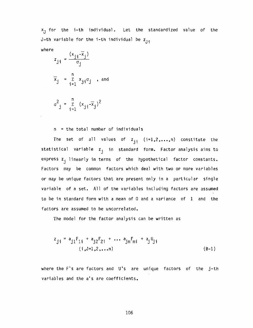
xJ for the i-th individual. Let the standardized value of the
J-th variable for the i-th individual be zJ i
where
z .. Jl
x. J
2 cr . J
(x .. -x.) Jl J =
n = L:
i
n = L:
;
cr· J
x .. cr. Jl J
,
2 (x .. -x.) Jl J
and
n = the total number of individuals
The set of all values of Z .• J 1
(i=1,2,. •• ,n) constitute the
statistical variable z· in standard form. Factor analysis aims to J
express Zj linearly in terms of the hypothetical factor constants.
Factors may be common factors which deal with two or more variables
or may be unique factors that are present only in a particular single
variable of a set. All of the variables including factors are assumed
to be in standard form with a mean of 0 and a variance of 1 and the
factors are assumed to be uncorrelated.
The model for the factor analysis can be written as
Zj; = aj1 F1i + aj2 F2i + ••• ajmFm; + ajUji (i ,J=1,2, ••• n) (B-1)
where the F's are factors and U's are unique factors of the j-th
variables and the a's are coefficients.
106

It can be shown by considering the variance of both sides of
Equation (19) above that the contribution of the factor FJ
to the
total variance is given by
n 2 l: a ..
i =1 ' J (B-2)
The communality of the i-th variable is defined to be the sum of
squares of the common factor coefficients and is given by
h2. = a2 +a2 + +a2 , il i2 ••• im (B-3)
The unique factor U. can be decomposed into the variance due to , the specific factor (specific variance or specificity) and variance
due to errors in measurement (error variance or unreliabil'ity). The
complement of the error variance is known as the reliability of the
variable. With the unique factor decomposed, the model of factor
analysis can be written as
z. = a. 1F1+a. 2F2+ ••• +a. F +b.s.+c.E. , " 1m m " "
(i=I,2, ••• ,n)
yielding the relationship
1 = h. 2 + b. 2 + c. 2 , , ,
(B-4)
(B-5)
when variances are considered on both sides of Equation (B-4), since
107

the ZIS, F's, SiS, are all standard normal variables.
The basic problem of factor analysis is to determine the
coefficients aiJ of the common factors. The coefficients aiJ are usually known as the 'loadings' of the factors.
The fundamental idea of factor analysis is that the correlation
matrix R can be decomposed into a product of a matrix A and its
transpose and the fundamental equation is given by
R = AAI (B-6)
where
R = the correlation matrix
A = the matrix of factor loadings with a typical element as
aiJ , and
AI = the transpose of A
Factor analysis consists of three steps which are (a) preparation
of correlation matrix (b) extraction of initial factors (c) rotation
of factors to reach the terminal solution. The first step involves
calculating the appropriate measurement of association between the
relevant variables and is relatively easy. The second step in factor
analysis is to obtain the factor constants on the basis of the
correlation matrix. Factors are extracted by more than one method but
only the principal factor method is described here.
The principal factor method begins with extracting the first
factor Fl such that its contribution to the communalities of the
variables is as great as possible. Then the residual correlations
after the first factor extraction are obtained. The second factor
F2 which is orthogonal to or independent of Fl is obtained
108

such that it contributes most to the residual communality and so on
until all of the communality is exhausted. The first factor is
obtained so that the sum of the contributions of the factor to the
total communality is given by
(B-7 )
is a maximum under the conditions.
(i, j=I,2, ••• n) (B-8)
where the correlation r. , = r, , and r· , is the communality 1J J1 11 h,2 of the variable zi' 1
S1 is maximized using Lagrange multipliers. It can be shown
that the maximization leads to the conditions given by
...
= 0
(B-9)
which is the characteristic equation. The largest root Al leads to
solution of a;j for the first factor.
The first factor residuals are given by
( r, ,) R ' d 1 = r l' J' - a l' 1 aJ'1 1J eS1 ua (B-I0)
109

It can be shown that Factor analysis does not yield a unique
solution to the matrix equation R = AA'. There are an infinite number
of methods of decomposing R as a product of the factor matrices, a
matrix and its inverse.
For example, let the A matrix or the matrix of unrotated loadings
be given by the 4 x 2 matrix A
A =
(B-l1 )
and a matrix (2x2) be given by
= [
COS ¢
-sin ¢
sin
(B-12) cos
The product AA = B given by
B = bl1 b12 = AA
b21 b22 b31 b32 b41 b42 (B-13)
If R = AA I , the value of BB'is
BB I = (AA)(AA) I = AAA' A I = AA I (B-14)
110

since 8.8.' =
[
COS ¢
-sin ¢
=
sin ¢] [COS ¢ cos ¢ .s in ¢
= I
-sin
cos
where I is the identity matrix of dimension 2.
:J
The second coefficients of factor F2 are obtained by
considering the matrix of residual correlations and maximizing the
quantity
+ ••• + (B-15)
which is the sum of the contribution of F2 to the residual
communality and so on. It can be shown that the second largest
eigenvalue of the original correlation matrix R leads to the solution
of the second factor and so on.
The third step involves rotation of the factor loadings matrix
obtained "initially into a mathematically equivalent matrix which
yields factor constants that are more useful for scientific purposes
than unrotated factor constants. It was seen that since R = AA' = BB'
irrespective of the value of ¢ this step is not difficult.
There are several methods of rotation. The 'varimax' method of
combined rotation used in this study simplifies the columns of the
factor loadings of ease factor in order to make interpretation a
simple matter. The factor loadings can be seen as the correlations
between the variables and the hypothetical factor. The variables that
111

have high loadings for each factor are studied carefully. If a
variable does not have high loadings for the first few factors that
account for most of the variability of the data, it can be eliminated
if needed.
In this study, in the 'Factor Procedure ' of SAS, the options of
the principal axis method and rotation by the varimax method were
used.
112

APPENDIX C
CLUSTER ANALYSIS
In cluster analysis no assumption is made about the group
structure. Grouping a set of objects or entities is done on the basis
of similarity or distances. For the purpose of clustering the
distance Id l between 2 m -dimensional observations ~ = (xl' ~,
xm)l and ~ = (Yl' Y2' ••• Ym)l is given by the distance, d, where
(C-l)
Clustering is subjective to some extent and the researcher is
expected to know enough about the background of the problem to be able
to differentiate between bad and good groupings. There are many ways
of clustering a set of objects with different clustering algorithms.
The ICluster l Procedure of SAS performs an agglomerative hierarchial
cluster analysis and the IFastclus l Procedure can be used for large
data sets with only two or three pairs over the data. In the Fastclus
procedure the observations belong to one and only one cluster.
Fastclus uses Arderberg1s (88) I nearest centroid sorting l • A very
brief discussion of the agglomerative hierarchial clustering method
and centroid methods is given below.
In hierarchial clustering agglomerative hierarchial methods or a
divisive hierarchial method may be used. Agglomerative hierarchial
113

procedures begin with the individual entities with as many clusters as
objects. The nearest or most similar objects are first grouped and
then the initial groups are again merged according to similarities or
distances. Thus, eventually all subgroups are fed into one single
group or cluster. Divisive hierarchial methods work in the reverse
way. The total set of objects initially start as one group and then
divide into two subsets such that the entities in one group are as
distant from the second group as possible. These subsets are again
divided into dissimilar subsets and so on until finally there are as
many groups or clusters as there are entities.
There are generally four steps necessary for aggl omerati ve
hierarchial clustering. The first step starts with n clusters, one
for each object and a nxn symmetric matrix of distances or
similarities is calculated. Let the distance matrix be denoted by D =
Step two is a search of the distance matrix for the
nearest or most similar pair of clusters. The distance between the
two nearest clusters C1 and C2 can be denoted by
d C1C2
The thi rd step is to merge cl usters C1 and
C2• Denote the newly formed cl uster by (C1 ' C2) • Now the
distance matri x can be updated by deleting the rows and columns
corresponding to cl uster C1 and C2 and by adding a row and
column giving the distances between cl uster (C1 ' C2) and the
remaining clusters. Steps two and three are repeated n-1 times to
obtain a single cluster in the end. The identity of clusters that are
merged into and the distances or similarities at which they are merged
can be recorded.
114

From the cluster procedure of SAS, one can obtain at each step
the (i) number of clusters (ii) the maximum di~tance between the
observations in a cluster which is called the maximum diameter of a
cluster (iii) the number of distances within clusters less than the
maximum diameter (iv) the total number of distances less than the
maximum diameter and (v) the ratio of steps (ii) and (v). A good
grouping is indicated when a local peak is seen for the value of the
ratio in step (v).
In the 'Fastclus ' procedure, a set of point cluster seeds are
selected by an initial guess as the means or centroids of the
clusters. Each object in the set is assigned to the nearest seed to
yield tempora~ clusters whose means replace the initial seeds. The
process is repeated until no further changes take place in the
cluster. In the cluster procedure, Euclidean distances are used as
the basis to assign observations to groups.
115


APPENDIX D
DISCRIMINANT ANALYSIS
Discriminant analysis is concerned with analysis of groups of
populations or data sets. One of the purposes of discriminant
analysis is to construct classification schemes based on a set of m
variables to classify a new member to one of the predetermined groups.
The analysis can also be used to test for mean group differences and
to describe the overlap among groups. The usual assumptions of
discriminant analysis are the following (~).
(1) The groups must be discrete and identifiable,
(2) One should be able to describe each observation by a set of
measurements on the m variables, and
(3) These discriminating variables must have a multivariate
normal distribution. (Testing for normality is given in
Appendix E)
The aim of discriminant analysis in this study was to develop a
classification model to categorize an object on the basis of the
profile of its characteristics to one of the groups determined by the
cluster analysis. The theoretical approach to this problem of
deciding the group to which an object belongs is to undertake that
action which minimizes the average loss (risk) due to misclassifi
cation. The word 110ss1 is used in place of lerror' and the loss
function is the measure of error. The risk function is the average
116

loss for a given loss function (103).
In the case of two populations 'lT1 and if
denotes the loss associated with taking action a. 1
when state of nature 'IT. prevails, the loss \matrix can be written' J
as
Loss Matrix for Classification
State of nature Action z belongs to z belongs to
where c .. is the cost of misclassifying an object which actually lJ
belongs to the i-th population into the J-th population (i, j=1,2).
If p denotes the risk p = Expected Loss = E [L(ai,'lTJ)J. The
rule of classification is developed so as to minimize the risk (~).
The 'Discrim' Procedure of SAS (80) computes 1 i nea r
discriminant functions for classifying observations into two or more
groups on the basis of numerical values. The classification criterion
is by a measure of generalized squared distance (p) which can be based
on either the within group variances or the pooled covariance matrix
after prior probabilities of the groups are accounted for. A new
observation object is placed in the class from which it has the
smallest generalized squared distance. The generalized squared
117

distance 2 o i C~J for a new object ~(mx1) when costs of
misclassification are ignored is given by
0.2(Z) = (z-x.)IS.-1(z-x.) + lnIS.I- 2 lnlp.1 1 - - -1 1 --1 1 1
(0-1)
where
z = the vector of variables for v, the new object to be
cl ass ifi ed,
x. = the vector of means of variables in group i, -1
Si = the covariance matrix for group i,
5.-1 1
Is; I =
=
=
the
the
the
inverse of 5i determinant of 5.,
1 and
prior probability of assignment to group i given
the ratio of the number of observations in group
the sum of the number of observations in all
groups.
by
i to
the
When the covariance matrices of all groups are not equal, a
quadratic discriminant function is the result. If the covariance
matrices are equal, a linear discriminant function is obtained.
The classification rule of assigning an observation based on the
probability of its belonging to a particular group gives the same
results as that based on assigning to a group based on the smallest
generalized distance. The posterior probability of an observation z
belonging to group i (;=1,2,... groups) is given by
P. (z) = 1-
2 exp[-O.5 O. (z)] 1 -
(0-2 )
118

If setting i = w produces the smallest value of D2. (z) 1-
or the
largest value of Pi(~) then the observation is assigned to
population or group w.
The discriminant function developed can be judged or evaluated as
to its performance by the number of misclassifications that result
when the function is used. Fewer misclassifications indicate a better
discriminating function. The SAS 'Discrim ' Procedure yields the
number of misclassified observations for both the linear and quadratic
discriminant functions. When the within-covariance matrices are
equal, the linear discriminant function can be calculated from the SAS
output which also prints posterior probabilities of membership in a
group. For the quadratic discriminant function, SAS yields
classification results, but not coefficients of the function. A
program using the Proc Matrix procedure (80) can be used to obtain
the quadratic function and posterior probabilities when covariance
matrices are not equal. A quadratic discriminant function in this
study included 98 quadratic terms, 14 linear terms and a constant.
The model was not found desirable because there were more parameters
estimated than the number of observations and it was difficult to
interpret.
One of the assumptions of discriminant procedure is that each of
the variables has a normal distribution. The variables can be tested
for normality using the 'univariate ' procedure of SAS discussed in the
following Appendix (E).
119

APPENDIX E
TESTING FOR NORMALITY
The univariate procedure of SAS tests for the normality of a
variable when the I normal I option is specified. SAS tests the data
against a normal distribution with mean and variance equal to the
sample mean and variance. The Kolmogorov-Smirnov D-Statistic is used
when the sample size n is greater than 50 and the W-statistic when n
is less than 50 to test the null hypothesis that the data values are a
sample from a normal distribution. The D and W statistics are briefly
discussed later in this appendix. The associated probability that the
data comes from a normal distribution is also printed. The output
also consists of a stem and leaf plot, box plot and normal probability
plot which are all also briefly described below to help decide whether
the sample comes from a normal distribution.
Stem and Leaf Plot
The Stem and Leaf Plot forms a picture of the frequency
distribution that is almost the same as the histogram except that it
is rotated by 90 degrees. It is a pictorial representation of the
distribution that is adequate for exploratory purposes (104).
Box Plot
A Box Plot is a graphical display that indicates the center or
120

location of the median. The box consists of the middle 50% of the
observations. The position of the median line indicates the skewness
if any. Since the distribution mean and median are at the same
position in a normal distribution, a discrepancy from normal
distribution can be observed by the position of the median in the box.
The outliers or extreme pOints are also graphed. The number of
outliers also indicates non-normality (104).
Kolmogorov-Smirnov Test
The Kolmogorov-Smirnov O-Statistic is often used to test the
goodness of fit of continuous data. The test involves two cumulative
distribution functions - the hypothesized and the observed. Let F(x)
be used to denote the probability that X is less than or equal to x,
or F(x) = P(X ~ x).
If FO(x) represents the cumulative hypothesized distribution
and S(X) the cumulative sample distribution, the aim of the
Kolmogorov-Smirnov test is to determine whether the disagreement
between FO(x) and S(x) is enough to doubt the hypothesis that the
sample comes from the hypothesized distribution (105). The test
statistics are given by
o = sup IS(x) - FO(x) I
which is read as "0 equals the supreme over all xi of the absolute
value of the difference S(x) - FO(x)". Graphically 0 is the
greatest vertical distance between S(x) and FO(x). The critical
values for decision are obtained from tables given in standard
non-parametric text books.
121

Normal Probability Plot
Normal probability graph paper is designed so that the plot of a
cumulative normal distribution is a straight line. Substantial
departures from a straight line indicate that the distribution is
non- norma 1 (83).
W-Statistic
The W-statistic is used for testing normality when the sample
size is less than or equal to 50. Shapiro and Wilk (106) discuss an
analysis of variance test for normality with the W-statistic which is
obtained by dividing the square of an appropriate linear combination
of the sample order statistics by the usual symmetric estimate of a
variance. The W-statisic is defined by
where
y =
where
... random observation, and
n S2 = l: (y __ y)2
- 1 ' ,=
(E-1)
is a vector of ordered
(E-2)
denote an ordered random sample of size n from the normal distribution
with a mean of 0 and a variance of 1 such that
(i=1,2, ••• m)
122

and b is the best linear unbiased estimate of the slope of a linear
regression relating the ordered observations, Yi ' to the expected
values mi of the standard normal order statistics. The constant b
is given by
(E-3)
where the coefficients a, and the percentile points of distribution of
W, are obtained from tables (106). Small values of W indicate non
norma 1 ity.
123

APPENDIX F
LOGISTIC REGRESSION
Some of the terms used in logistic regression are explained here.
Likelihood Function (103)
Consider n random variables xl' x2 ' Their
likelihood function may be defined as their joint density given by
which can be taken to be the function of 8.
If the sample is taken from the density f(x;6), then the
likelihood function is given by
The likelihood function yields the Ilikelihood l that the random
variable e assumes a particular value xl' x2 ' It is
the val ue of a density functi on and a probabil ity for di screte random
variables.
Maximum Likelihood Estimators (103)
Let be the observed values in a
124

sample which supposedly has come from a population with joint density
given by
f ( xl' x2' ••• x n; 8) xl'··' xn
where e is unknown.
The aim is to know S or the density from which this particular
sample is Imost likely' to have come. We wish to find the value of 8,
say 80
which maximizes the likelihood function L(8;x I, x I, •••
X I) sometimes the logarithm of the likelihood given by log L(8) is
considered since L(S) and log L(8) have their maxima for the same
val ue of e.
The maximum likelihood estimator is the solution of the equation
given by
dL(8) = a de (F-l)
If there are p parameters to be considered, the likelihood
function is given by
n = .IT f(n i 'Sl,82, .•• ,ep)
1=1 (F-2)
and maximum likelihood estimators are obtained by solving the
equations
aL( = a (i=1,2, .. qp) (F-3)
125

It is often better to work with the logarithm of the likelihood
function.
Likelihood Ratio
Likelihood ratio is the ratio of two likelihood functions or
their logarithms.
Logistic Regression ,
Often when the response variable is an indicator variable, the
shape of the response function is not linear but curvilinear (82).
A graphical representation of the response function which is found to
be adequate when the dependent variable is bina~ is given in Figure
(7). As can be seen from Figure (7) this response function is shaped
like a letter S and has asymptotes at 0 and 1.
Logistic regression does not require the assumption that the
variables are normally distributed as is the case with discriminant
analysis. Also costs of misclassification do not enter the picture as
they do in discriminant analysis. In this study, two groups of
bridges were determined as belonging to Imore-safe' and 'less-safe l
categories by cluster analysis. If z is an indicator variable with
z=l for bridges in the more-safe group and with z=O for bridges in the
less-safe group, it is possible to fit a logistic regression model.
This model can be used to predict the probability of a bridge being
'safe ' because in this case, a II' represents a safe bridge. The
probability that is calculated directly by the model can serve as an
index of safety and is always between 0 and 1.
126

Let Pi be denoted as the probability of a bridge being safe.
In order to relate the probability of safety of the dichotomous
(categorical) response variable y to the m independent variables
Xi (i=1,2, ••• m), the following model is used:
where
Pi = y /l +y, and
1-P i = 1/l+y
Yi
b. J
The
A. 1
=
m = exp L b·x··
j=1 J 1 J
= unknown coefficients that need to be determined.
quantity A. is defined as 1
m In(p./(l-p.) = 1:: b.x ..
1 1 j=1 J lJ
The variable A. is called the logistic transform of 1 Pi
(F-4)
(F-5)
(F-6)
and
Equation (F-6) gives the linear logistic model. The probability of
safety can be obtained from Equation (F-4) or (F-6). The b. 1
coefficients can be estimated by using the maximum likelihood method.
The logarithm of the likelihood function can be obtained as
=
nl n m 1:: b.t. - 1:: In[l+exp( 1:: b.x .. )]
j=1 J J i=1 j=1 J lJ
where Y1' Y2'
the n objects
Yn
(~.Q)
are the
and
127
=
dichotomous n 1:: x··
i =1 1 J
( F-7)
observations on
Yi. The maximum

likelihood estimates of the b 's J that maximize the logarithm of
the likelihood function are obtained by solving iteratively the
following m equations simultaneously:
m n
t.- E J i=l
x .. exp( E b.x .. } lJ =1 J 1J
m 1 + exp( E b~x .. }
j=l J lJ
(j=1,2, ... ,m)
= 0
(F-8)
The 'logit' procedure in SAS due to Harrell (21t 92) solves
the above Equation (F-8) iteratively and computes the maximum
likelihood estimates for the regression coefficients. This model can
also be fitted in a stepwise technique based on a strategy that
determines the best variable to be added at any given stage with very
few calculations. If the stepwise option is not used t the maximum
likelihood estimates for the parameters associated with each
independent variable are calculated and printed. The output includes
of the model likelihood ratio, the model Chi-Square t and the degrees
of freedom of the model. The model log likelihood ratio Chi-Square is
defined to be twice the difference in the log likelihood of the
current model from the likelihood based on the intercept alone. A
statistic 'R' which indicates the predictive ability of the model is
also obtained in the output. The 'R' statistic is similar to the
multiple correlation coefficient after a correction is made to account
for the number of parameters estimated.
equation
R2 = (model CHi-stuare - 2m) [-2L e)]
128
It is obtained from the
(F-9)

where m is the number of variables in the model excluding the
intercept and L(8) is the maximum log-likelihood with only intercept
in the model.
IIpartial Risli are also computed for each independent variable in
the model and are given by
(F-lO)
and carry the sign of the corresponding regression coefficient (2£).
The output of the logistic procedures contains the fraction of
the IIconcordant pairs of predicted probabilities and responses. 1I In
other words, all pairs of observations having different values of y
are considered and the number of pairs are counted in which the
observation with the larger y has a higher predicted probability than
does the observation with the smaller y. The ratio of the number of
pairs in which the predicted probabilities are concordant with the
dependent variable value to the total number of possible pairs gives
the fraction of observations that are concordant. If this value is
denoted by ICI and the fraction of discordant pairs is denoted by Id'
(d=l-c if there are no ties); an index of rank correlation between the
predicted probabilities and dependent variable is given by c-d. This
rank correlation is very similar to Kendall IS Rank correlation and is
actually Somer's D-Statistic, both of which are discussed below.
These measures indicate the goodness of the model.
129

Kendall's Tau Rank Correlation Coefficient and Somer's 0
Kendall's Tau is a non-parametric statistics that yield a measure
of correlation between two variables x and y. It is based on the
ranks of observations and assumes values between -1 and +1. Two pairs
and
be concordant if the difference between xl
same direction as the difference between Y1
said to be concordance if when xl > x2' then
are said to
is in the
There is
>
or when xl < x2 then we have also Y1 < Y2. The pairs
are said to be discordant if the directions of difference are not
same. The procedure begins by arranging x-ranks in order from 1 to n
and pair with the corresponding of y ranks. Then the strategy
consists of obtaining the number of consistencies or concordance say,
c, and the number of discrepancies or discordance say, d, in the
paired ranks. The ratio of the number of concordant pairs to the
total number of possible consistencies in the case of perfect
concordance yields Kendall's rank correlation coefficient.
There is an adjustment in calculating the value of Kendall's Tau
in case of ties in the rank (92). Somer's D-Statistic is similar to
Kendall's Tau except slightly different in adjusting for ties (107).
130


APPENDIX G
LISTS OF BRIDGE DATA AND SITE LOCATIONS
Table 1G. List of Bridge Sites
DISTRICT BRIDGE 1.D. COUNTY BRIDGE NO.
2 C Tarrant 220
2 D Wise 249
2 E Erath 73
2 F Erath 73
2 G Hood 112
2 H Erath 73
9 A Bell 14
9 F Bell 14
9 G Bell 14
10 D Henderson 108
10 F Anderson 001
10 G Gregg 93
10 H Van Zandt 234
10 I Anderson 001
10 C Henderson 108
11 C Tri nity 228
11 D Trinity 228
11 E Houston 114
11 F San Augustine 203
131

Table 1G. List of Bridge Sites (cont'd)
DISTRICT BRIDGE !.D. COUNTY BRIDGE NO.
12 A B razor; a 20
12 G Harris 102
12 I B razori a 20
12 J Brazoria 20
12 K Harri s 102
12 L Montgomery 170
13 A Calhoun 29
13 B Colorado 45
13 F Dewitt 62
13 D Fayette 76
13 E Gonzales 90
13 C Dewitt 62
14 A Bastrop 11
14 C Llano 150
14 E Bastrop 11
14 F Hays 106
14 D Williamson 246
14 H Williamson 246
14 I Williamson 246
16 D Refugio 196
16 E Refugio 196
132

Table IG. List of Bridge Sites (cont'd)
DISTRICT BRIDGE I.D. COUNTY BRIDGE NO.
16 F San Patricio 205
16 G San Patricio 205
18 B Denton 61
18 C Kaufman 130
18 D Navarro 175
20 B Hard; n 101
20 F Jasper 122 .. 20 H Liberty 146
20 I Hardi n 101
3 B Wi chita 243
3 C Wil barger 244
3 D Wil barger 244
3 E Wil barger 244
3 F Young 252
3 G Young 252
3 H Montague 169
4 A Hartley 104
4 B Hemphill 107
4 D Oldham 180
4 E Oldham 180
4 F Randa 11 191
133

Table 1G. List of Bridge Sites (cont'd)
DISTRICT BRIDGE 1.0. COUNTY BRIDGE NO.
7 A Coke 141
7 G Tom Green 226
7 H Tom Green 226
7 I Tom Green 226
21 A Kenedy 66
21 B Duval 67
21 0 Hidalgo 109
21 G Webb 240
21 H Zapata 253
21 I Zapata 253
22 A Ki nney 136
22 B Kinney 136
22 C Maverick 159
22 0 Uvalde 232
22 E Val Verde 233
22 F Val Verde 233
22 H Zavala 254
134

Table2G.Fl - F12 Rating Data-for all 78 Bridges
Bri dge Site Fl F2 F3 F4 F5 F6 F7 F8 F9 FlO F11 F12
2C--Tarrant 220 5 5 5 5 5 1 1 4 3 3 1 2
2D--Wise 249 5 3.75 2.50 5 5 5 1 5 2 5 3 2
2E--E rath 73 5 5 1. 25 5 5 2 1 4 4 2 3 3
2F--E rath 73 4.5 2.50 0.00 4 4 3 1 5 3 4 3 3
2G--Hood 112 5 5 2.50 5 5 5 1 4 2 2 3 2
2H--Erath 73 4.5 2.50 3.75 5 5 5 1 5 4 4 3 3
9A--Bell 14 5 1. 25 1. 25 5 5 1 2 4 3 4 3 3
9F--Bel1 14 5 1. 25 2.50 5 5 1 3 5 2 3 1 2
9G--Bell 14 5 3.75 0.00 3 1 5 1 2 1 4 1 2
10D--Henderson 108 5 2.50 1. 25 5 5 5 2 4 2 2 1 2
10F--Anderson 001 4.25 1.25 0.00 5 5 2 5 5 4 4 1 2
10G--Gregg 93 5 1. 25 1. 25 5 5 5 5 4 5 4 3 2
10H--Van Zandt 234 2.5 2.50 0.00 5 3 1 5 5 4 4 1 2
10I--Anderson 001 5 3.75 2.50 5 5 5 1 4 1 1 1 2
10C--Henderson 108 5 2.50 1. 25 5 5 5 2 4 2 2 1 2
11C--Trinity 228 5 2.50 1. 25 5 4 5 1 4 3 3 1 1
110--Tri nity 228 5 2.50 1. 25 5 5 5 1 4 3 3 2 2
11E--Houston 114 5 3.75 1. 25 5 5 5 5 5 5 5 1 2 \
11F--San Aug 203 5 2.50 1. 25 5 5 5 2 5 4 4 1 1
12A--Brazoria 20 ,5 3.75 1. 25 5 1 5 1 4 4 4 3 2
12G--Harris 102 5 2.50 0.00 5 5 1 1 2 2 1 1 3
12I--Brazoria 20 5 3.75 1. 25 5 5 1 1 4 4 3 1 3
12J--Brazoria 20 5 1. 25 0.00 5 5 5 5 4 3 3 1 2
12K--Harris 102 5 1. 25 0.00 5 5 5 5 4' 4 4 3 2
135

Table 2G .. (Continued)
Bridge Site Fl F2 F3 F4 F5 F6 F7 F8 F9 flO Fll Fl2
12L--Montgmry 170 5 2.50 1. 25 5 5 5 5 4 2 2 3 2
13A--Calhoun 29 5 2.50 1. 25 5 5 5 2 5 3 5 4 1
13B--Colorado 45 5 2.50 0.00 5 1 4 1 4 2 2 2 3
13F--Dewitt 62 5 2.50 5 5 5 5 1 4 3 1 1 2
13D--Fayette 76 5 2.50 1. 25 5 3 4 1 4 3 2 1 2
13E--Gonzales 90 5 2.50 2.50 5 5 5 1 4 4 1 1 2
13C--Dewitt 62 5 2.50 3.75 5 4 5 1 4 3 1 2 2
14A--Bastrop 11 5 1. 25 1. 25 5 2 3 1 4 5 2 1 3
14~-Ll ana 150 5 2.50 1. 25 5 5 3 1 5 3 1 2 1
14E--Bastrop 11 4.5 1. 25 1. 25 5 .5 3 5 5 5 5 1 2
14F--Hays 106 5 2.50 1. 25 1 1 1 5 5 3 1 1 3
14D--Wmson 246 5 5 2.50 5 5 3 5 5 5 5 1 2
14H--Wmson 246 5 5 2.50 5 5 4 1 5 4 4 1 2
14I--Wmson 246 5 5 5 5 2 5 1 4 4 3 1 2
16D--Refugio 196 5 2.50 3.75 5 3 3 3 4 2 4 3 2
16E--Refugio 196 5 2.50 5 5 5 5 3 4 2 4 4 2
16F--Sanpatricio 205 3.75 2.50 3.75 5 5 5 1 5 3 4 2 3
16G--Sanpatricio 205 3.75 2.50 3.75 5 5 5 1 5 3 4 2 3
18B--Denton 61 5 2.50 3.75 5 5 5 1 4 2 2 1 2
18C--Kaufman 130 5 3.75 2.50 5 1 4 1 4 2 3 3 3
18D--Navarro 175 5 5 0.00 5 5 5 1 5 5 5 1 3
20B--Hardin 101 5 2.50 1. 25 5 5 5 2 4 2 4 2 2
20F--Jasper 122 5 2.50 1.25 5 5 5 2 4 2 4 2 2
20H--Liberty 146 3.75 5 0.00 5 5 5 1 5 2 4 2 2
13q
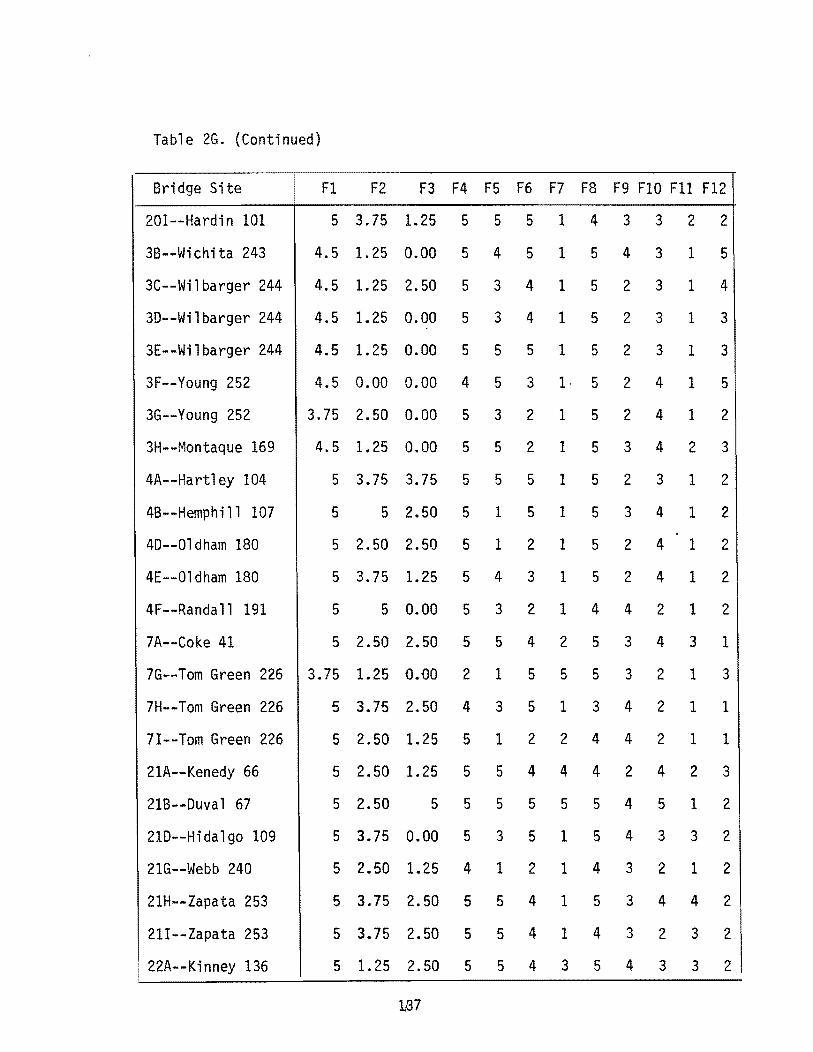
Table 2G. (Continued)
Bridge Site
20I--Hardin 101
3B--Wichita 243
3C--Wilbarger 244
3D--Wilbarger 244
3E--Wilbarger 244
3F--Young 252
3G--Young 252
3H--Montaque 169
4A--Hartley 104
4B--Hemphi 11 107
4D--Oldham 180
4E--Oldham 180
4F--Randa 11 191
7A--Coke 41
7G--Tom Green 226
7H--Tom Green 226
7I--Tom Green 226
21A--Kenedy 66
21B--Duval 67
21D--Hidalgo 109
21G--Webb 240
21H--Zapata 253
21I--Zapata 253
• 22A--Kinney 136
F1 F2 F3 F4 F5 F6 F7 F8 F9 FlO F11 F12
5 3.75 1.25 5 5 5 1 4 3 3 2 2
4.5 1.25 0.00 5 4 5 1 5 4 3 1 5
4.5 1.25 2.50 5 3 4 1 5 2 3 1 4
4.5 1.25 0.00 5 3 4 1 5 2 3 1 3
4.5 1.25 0.00 5
4.5 0.00 0.00 4
3.75 2.50 0.00 5
4.5 1.25 0.00 5
5 3.75 3.75 5
5 5 2.50 5
5 2.50 2.50 5
5 3.75 1.25 5
5 5 0.00 5
5 2.50 2.50 5
3.75 1.25 0.00 2
5 3.75 2.50 4
5 2.50 1.25 5
5 2.50 1.25 5
5 2.50 5 5
5 3.75 0.00 5
5 2.50 1.25 4
5 3.75 2.50 5
5 3.75 2.50 5
551 523 1 3
5 3 1· 5 2 4 1 5
321 524 1 2
521 5 342 3
551 523 1 2
151 534 1 2
121 524 1 2
431 524 1 2
321 442 1 2
542 5 343 1
1 555 321 3
351 342 1 1
1 224 4 2 1 1
5 444 2 4 2 3
5555451 2
351 543 3 2
1 2 1 4 3 2 1 2
541 5 344 2
541 432 3 2
5 1.25 2.50 5 5 4 3 5 4 3 3 2
187

)
Table 2G. (Continued)
Bridge Site F1 F2 F3 F4 F5 F6 F7 F8 F9 FlO Fll F12
22B--Kinney 136 5 2.50 1.25 5 5 3 3 5 4 t: 4 2 ,j
22C--Maverick 159 5 2.50 0.00 5 5 5 3 5 4 3 4 2
22D--Uvalde 232 5 3.75 0.00 5 5 4 1 5 5 4 1 2
22E--Val Verde 233 5 5 1. 25 5 5 2 1 5 4 1 1 1
22F--Val Verde 233 5 3.75 1. 25 5 1 4 1 5 4 2 2 1
22H--Zavala 254 5 3.75 0.00 5 5 5 1 5 4 4 1 2
138

• • • Table 3G. Data for New Bridge Safety Index
BRIDGE KADT, BRIDGE BRIDGE WIDTH, 1000 SPEED, LENGTH,
NO. ID FT VEH/DAY MPH FT F9 F6 F7
1 C2 30.00 4.30 50 125 3 1 2 D2 28.00 3.20 60 910 2 5 1 3 E2 30.00 7.30 55 240 4 2 1 4 F2 22.00 0.90 55 255 3 3 1 5 G2 30.00 7.60 55 825 2 5 1 6 H2 22.00 0.90 55 1105 4 5 1 7 A9 26.00 3.92 55 720 3 1 2 8 F9 25.80 2.65 60 3632 2 1 3 9 G9 23.50 2.13 45 316 1 5 1
10 D10 28.00 5.14 60 2401 2 5 2 11 FlO 21.75 1.38 60 819 4 2 5 12 G10 26.00 4.70 55 450 5 5 5 13 HlO 19.30 0.62 55 50 4 1 5 14 110 28.00 4.51 55 1723 1 5 1
I--' 15 ClO 28.00 5.14 55 1920 2 5 2 w 16 D11 23.80 4.00 55 2884 3 5 1 ~
17 E 11 29.00 0.90 55 282 5 5 5 18 F11 30.00 1. 70 55 640 4 5 2 19 A12 27.70 7.14 55 1040 4 5 1 20 G12 28.00 17.20 55 1261 2 1 1 21 112 25.60 6.67 55 2416 4 1 1 22 J12 23.40 6.99 55 75 3 5 5 23 K12 30.75 14.78 60 303 4 5 5 24 L12 25.80 6.52 60 1647 2 5 5 25 A13 30.00 3.30 55 520 3 5 2 26 B13 25.50 6.70 55 1041 2 4 1 27 F13 23.70 3.70 55 1295 3 5 1 28 D13 25.60 7.80 55 1414 3 4 1 29 E13 23.80 5.60 55 1426 4 5 1 30 C13 23.70 3.70 55 782 3 5 1 31 C11 23.70 4.00 55 962 3 5 1 32 A14 26.00 7.50 40 1124 5 3 1 33 C14 24.00 7.50 40 876 3 3 1 34 E14 22.00 0.80 55 150 5 3 5 35 F14 24.00 3.20 40 150 3 1 5 36 D14 28.00 1.80 60 510 4 4 1 37 H14 28.00 1.80 60 501 4 4 1 38 114 27.50 3.68 55 411 4 5 1 39 D16 29.80 5.50 60 247 2 3 3

• • • Table 3G. (cont'd)
BRIDGE KAOT, BRIDGE BRIDGE WIDTH, 1000 SPEED, LENGTH,
NO. ID FT VEH/OAY MPH FT F9 F6 F7
40 E16 30.00 5.50 60 601 2 5 3 41 F16 21.80 2.30 55 1997 3 5 1 42 G16 21.90 2.20 55 798 3 5 1 43 B18 24.00 7.80 55 804 2 5 1 44 C18 26.00 3.70 55 849 2 4 1 45 018 26.00 2.80 55 482 5 5 1 46 B20 28.40 7.47 60 303 2 5 2 47 F20 28.40 7.47 55 1604 2 5 2 48 H2O 21.30 1.40 55 275 2 5 1 49 120 28.00 7.00 60 607 3 5 1 50 B03 22.00 2.40 55 397 4 5 1 51 C03 24.00 2.20 55 1852 2 4 1 52 D03 24.00 2.20 55 362 2 5 1 53 E03 24.00 2.20 50 161 2 5 1 54 F03 22.00 1.60 55 839 2 3 1 55 G03 20.00 0.70 55 1063 2 2 1
I-' 56 H03 22.00 1.60 55 2036 3 2 1 -I:» 0 57 A04 30.00 2.00 55 440 2 5 1
58 B04 27.00 3.60 55 2926 3 5 1 59 004 27.80 1.50 55 250 2 2 1 60 E04 27.00 1. 60 55 1627 2 3 1 61 F04 30.00 5.20 55 334 4 2 1 62 A07 30.20 1. 70 55 886 3 4 2 63 G07 21.60 2.10 50 335 3 5 5 64 H07 30.00 11.00 55 1130 4 5 1 65 107 30.00 4.30 55 1143 4 2 2 66 A21 39.90 3.80 55 100 2 4 4 67 B21 44.00 1.50 55 205 4 5 5 68 021 30.00 1.50 55 3181 4 5 1 69 G21 25.50 3.90 55 189 3 2 1 70 H21 27.60 2.00 55 1190 3 4 1 71 121 27.60 3.20 55 1850 3 4 1 72 A22 34.90 2.20 55 1431 4 4 3 73 B22 38.00 2.20 55 66 4 3 3 74 C22 31.00 1.60 55 120 4 5 3 75 022 27.30 1.80 55 341 5 4 1 76 E22 27.70 1.00 55 1310 4 2 1 77 F22 30.00 1.50 55 5462 4 4 1 78 H22 25.60 2.00 55 1505 4 5 1

I-' ~ I-'
Range of
Variables
Maximum
Minimum
Table 4G. Range of Variables in New Bridge Safety Index
Bridge Width,
Ft
44.0
19.3
KADT 1000 Veh
Day
17.20
0.70
Speed, MPH
60
40
Length, Ft
5462
50
F9
5
1
F6
5
1
F7
5
1