SplitGuard: Detecting and MitigatingTraining-Hijacking Attacks in Split Learning

Ege ErdoganDept. of Computer Engineering

Koc UniversityIstanbul, Turkey

eerdogan17@ku.edu.tr

Alptekin KupcuDept. of Computer Engineering

Koc UniversityIstanbul, Turkeyakupcu@ku.edu.tr

A. Ercument CicekDept. of Computer Engineering

Bilkent UniversityAnkara, Turkey

cicek@cs.bilkent.edu.tr

Abstract—Distributed deep learning frameworks, such as splitlearning, have recently been proposed to enable a group of par-ticipants to collaboratively train a deep neural network withoutsharing their raw data. Split learning in particular achieves thisgoal by dividing a neural network between a client and a server sothat the client computes the initial set of layers, and the servercomputes the rest. However, this method introduces a uniqueattack vector for a malicious server attempting to steal the client’sprivate data: the server can direct the client model towardslearning a task of its choice. With a concrete example alreadyproposed, such training-hijacking attacks present a significantrisk for the data privacy of split learning clients.

In this paper, we propose SplitGuard, a method by which asplit learning client can detect whether it is being targeted by atraining-hijacking attack or not. We experimentally evaluate itseffectiveness, and discuss in detail various points related to itsuse. We conclude that SplitGuard can effectively detect training-hijacking attacks while minimizing the amount of informationrecovered by the adversaries.

Index Terms—machine learning, data privacy, split learning

I. INTRODUCTION

As neural networks, and more specifically deep neuralnetworks (DNNs), began outperforming traditional machinelearning methods in tasks such as natural language processing[1], they became the workhorses driving the field of machinelearning forward. However, effectively training a DNN re-quires large amounts of computational power and high-qualitydata [2]. On the other hand, relying on a sustained increasein computing power is unsustainable [3], and it may not bepossible to share data freely in fields such as healthcare [4],[5].

To alleviate these two problems, distributed deep learningmethods such as split learning (SplitNN) [6], [7] and federatedlearning (FL) [8]–[10] have been proposed. They fulfill theirpurpose by enabling a group of data-holders to collaborativelytrain a DNN without sharing their private data, while offload-ing some of the computational work to a more powerful server.

In FL, each client trains a DNN using its local data, andsends its parameter updates to the central server; the serverthen aggregates the updates in some way (e.g. average) andsends the aggregated results back to each client. In SplitNN,a DNN is split into two parts and the clients train in a round-robin manner. The client taking its turn computes the first fewlayers of the DNN and sends the output to the server, who then

computes the DNN’s overall output and starts the parameterupdates by calculating the loss value. In both methods, noclient shares its private data with another party, and all clientsend up with the same model.

Motivation. In SplitNN, the server has control over theparameter updates being propagated back to each client model.This creates a new attack vector, that has already been ex-ploited in an attack proposed by Pasquini et al. [11], for amalicious server trying to infer the clients’ private data. Bycontrast, this attack vector does not exist in federated learning,since the clients can trivially check if their model is alignedwith their goals by calculating its accuracy. The same processis not possible in split learning, since the adversary can traina legitimate model on the side using the clients’ intermediateoutputs, and use that model for a performance measure. Infact, any such detection protocol that expects cooperation fromthe server is doomed to failure through the server’s use of alegitimate surrogate model as described.

Contributions. Our main contribution in this paper isSplitGuard, a protocol by which a SplitNN client can detect,without expecting cooperation from the server, if its localmodel is being hijacked. We utilize the observation that if aclient’s local model is learning the intended task, then it shouldbehave in a drastically different way when the task is reversed(i.e. when success in the original task implies failure in the newtask). We demonstrate using three commonly used benchmarkdatasets (MNIST [12], Fashion-MNIST [13], and CIFAR10[14]) that SplitGuard effectively detects and mitigates the onlytraining-hijacking attack proposed so far [11]. We further arguethat it is generalizable to any such training-hijacking attack.

In the rest of the paper, we first provide the necessarybackground on DNNs and SplitNN, and explain some of therelated work. We then describe SplitGuard, experimentallyevaluate it, and discuss certain points pertaining to its use.We conclude by providing an outline of possible future workrelated to SplitGuard.

Supplementary code for the paper can be found athttps://github.com/ege-erdogan/splitguard.

arX

iv:2

108.

0905

2v1

[cs

.CR

] 2

0 A

ug 2

021

(a) With label-sharing. (b) Without label-sharing.

Fig. 1: Two different split learning setups. Arrows denote the forward and backward passes, starting with the examples X , andpropagating backwards after the loss computation using the labels Y . In Figure 1a, clients send the labels to the server alongwith the intermediate outputs. In Figure 1b, the model terminates on the client side, and thus the clients do not have to sharetheir labels with the server.

II. BACKGROUND

A. Neural Networks

A neural network [15] is a parameterized function f : X ×Θ → Y that tries to approximate a function f∗ : X → Y .The goal of the training procedure is to learn the parametersΘ using a training set consisting of examples X and labels Ysampled from the real-world distributions X and Y .

A typical neural network, also called a feedforward neuralnetwork, consists of discrete units called neurons, organizedinto layers. Each neuron in a layer takes in a weightedsum of the previous layer’s neurons’ outputs, applies a non-linear activation function, and outputs the result. The weightsconnecting the layers to each other constitute the parametersthat are updated during training. Considering each layer as aseperate function, we can model a neural network as a chain offunctions, and represent it as f(x) = f (N)(...(f (2)(f (1)(x))),where f (1) corresponds to the first layer, f (2) to the secondlayer, and f (N) to the final, or the output layer.

Like many other machine learning methods, training aneural network involves minimizing a loss function. However,since the nonlinearity introduced by the activation functionsapplied at each neuron causes the loss function to becomenon-convex, we use iterative, gradient-based approaches tominimize the loss function. It is important to note that thesemethods do not provide any global convergence guarantees.

A widely-used optimization method is stochastic gradientdescent (SGD). Rather than computing the gradient from theentire data set, SGD computes gradients for batches selectedfrom the data set. The weights are updated by propagating theerror backwards using the backpropagation algorithm. Traininga deep neural network generally requires multiple passes overthe entire data set, each such pass being called an epoch. Oneround of training a neural network requires two passes throughthe network: one forward pass to compute the network’soutput, and one backward pass to update the weights. We will

use the terms forward pass and backward pass to refer tothese operations in the following sections. For an overviewof gradient-based optimization methods other than SGD, werefer the reader to [16].

B. Split Learning

In split learning (SplitNN) [6], [7], [17], a DNN is splitbetween the clients and a server such that the clients computethe first few layers, and the server computes rest of the layers.This way, a group of clients can train a DNN utilizing, butnot sharing, their collective data. Furthermore, most of thecomputational work is also offloaded to the server, reducingthe training cost for the clients. However, this partitioninginvolves a privacy/cost trade-off for the clients, with theoutputs of earlier layers leaking more information about theinputs.

Figure 1 displays the two basic modes of SplitNN, themain difference between the two being whether the clientsshare their labels with the server or not. In Figure 1a, clientscompute only the first few layers, and should share their labelswith the server. The server then computes the loss value,starts backpropagation, and sends the gradients of its firstlayer back to the client, who then completes the backwardpass. The private-label scenario depicted in Figure 1b followsthe same procedure, with an additional communication step.Since now the client computes the loss value and initiatesbackpropagation, it should first feed the server model with thegradient values to resume backpropagation.

For our purposes, it is important to realize that the servercan launch a training-hijacking attack even in the private-label scenario (Figure 1b). It simply discards the gradientsit received from the second part of the client model, andcomputes a malicious loss function using the intermediateoutput it received from the first client model, propagating themalicious loss back to the first client model.

The primary advantage of SplitNN compared to federatedlearning is its lower communication load [18]. While federatedlearning clients have to share their entire parameter updateswith the server, SplitNN clients only share the output of asingle layer. However, choosing an appropriate split depth iscrucial for SplitNN to actually provide data privacy. If theinitial client model is too shallow, an honest-but-curious servercan recover the private inputs with high accuracy, knowingonly the model architecture (not the parameters) on the clients’side. This implies that SplitNN clients should increase theircomputational load, by computing more layers, for strongerdata privacy.

Finally, SplitNN follows a round-robin training protocol toaccomodate multiple clients; clients take turn training with theserver using their local data. Before a client starts its turn, itshould bring its parameters up to date with those of the mostrecently trained client. There are two ways to achieve this:the clients can either share their parameters through a centralparameter server, or directly communicate with each other ina P2P way and update their parameters.

III. RELATED WORK

A. Feature-Space Hijacking Attack (FSHA)

The Feature-Space Hijacking Attack (FSHA), by Pasquiniet al. [11], is the only proposed training-hijacking attackagainst SplitNN clients so far. It is important to gain anunderstanding of how a training-hijacking attack might workbefore discussing SplitGuard in detail.

In FSHA, the atttacker (SplitNN server) first trains anautoencoder (consisting of the encoder f and the decoderf−1) on some public dataset Xpub similar to that of theclient’s private dataset Xpriv . It is important for the attack’seffectiveness that Xpub be similar to Xpriv. Without such adataset at all, the attack cannot be launched. The main ideathen is for the server to bring the output spaces of the clientmodel f and the encoder f as close as possible, so that thedecoder f−1 can successfully invert the client outputs andrecover the private inputs.

After this initial setup phase, the client model’s training be-gins. For this step, the attacker initializes a distinguisher modelD that tries to distinguish the client’s output f(Xpriv) fromthe encoder’s output f(Xpub). More formally, the distinguisheris updated at each iteration to minimize the loss function

LD = log(1−D(f(Xpub))) + log(D(f(Xpriv))). (1)

Simultaneously at each training iteration, the server directs theclient model f towards maximizing the distinguisher’s errorrate, thus minimizing the loss function

Lf = log(1−D(f(Xpriv))). (2)

In the end, the output spaces of the client model and theserver’s encoder are expected to overlap to a great extent,making it possible for the decoder to invert the client’s outputs.

Notice that the client’s loss function Lf is totally indepen-dent of the training labels, as in changing the value of the

labels does not affect the loss function. We will soon refer tothis observation.

IV. SPLITGUARD

We start our presentation of SplitGuard by restating anearlier remark: If the training-hijacking detection protocolrequires the attacker SplitNN server to knowingly take part inthe protocol, the server can easily circumvent the protocol bytraining a legitimate model on the side, and using that modelduring the protocol’s run. In the light of this, it is evident thatwe need a method which the clients can run during training,without breaking the flow of training from the server’s pointof view.

A. Overview

During training with SplitGuard, clients intermittently inputbatches with randomized labels, denoted fake batches. Themain idea is that if the client model is learning the intendedtask, then the gradient values received from the server shouldbe noticeably different for fake batches and regular batches.1

The client model learning the intended task means thatit is moving towards a relatively high-accuracy point on itsparameter space. That same high-accuracy point becomesa low-accuracy point when the labels are randomized. Themodel tries to get away from that point, and the classificationerror increases. More specifically, we make the following twoclaims (experimentally validated in Section V-B):

Claim 1. If the client model is learning the intended task,then the angle between fake and regular gradients will behigher than the angle between two random subsets of regulargradients.2

Claim 2. If the client model is learning the intended task,then fake gradients will have a higher magnitude than regulargradients.

Notation

PF Probability of sending a fake batchBF Share of randomized labels in a fake batchN Batch index at which SplitGuard starts runningF Set of fake gradientsR1, R2 Random, disjoint subsets of regular gradientsR R1 ∪R2

α, β Parameters of the SplitGuard score functionL Number of classesA Model’s classification accuracyAF Expected classification accuracy for a fake batch

TABLE I: Summary of notation used throughout the paper.

B. Putting the Claims to Use

At the core of SplitGuard, clients compute a value, denotedthe SplitGuard score, based on the fake and regular gradients

1Fake gradients and regular gradients similarly refer to the gradientsresulting from fake and regular batches.

2Angle between sets meaning the angle between the sums of vectors inthose sets.

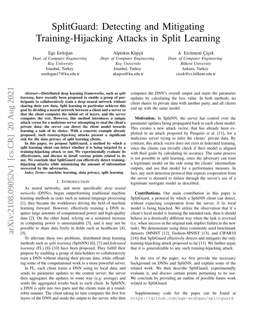
Fig. 2: Overview of SplitGuard, comparing the honest trainingand training-hijacking scenarios. Clients intermittently sendtraining batches with randomized labels, and analyze thebehavior of their local models visible from their parameterupdates.

they have collected up to that point. This value’s history is thenused to reach a decision on whether the server is launchingan attack or not. We now describe this calculation process inmore detail. Table I displays the notation we use from hereon.

Starting with the N th batch during the first epoch of train-ing, with probability PF ,3 clients send fake batches with theshare BF ∈ [0, 1] of the labels randomized. Upon calculatingthe gradient values for their first layer, clients append the fakegradients to the list F , and split the regular gradients randomlyinto the lists R1 and R2, where R = R1∪R2. To minimize theeffect of fake batches on model performance, clients discardthe parameter updates resulting from fake batches. Figure 2displays a simplified overview of the protocol, and Algorithm1 explains the modified training procedure in more detail.The MAKE_DECISION function contains the clients’ decison-making logic and will be described later in Algorithm 3.

To make sure that none of the randomized labels getsmapped to its original value, it is a good idea to add to eachlabel a random positive integer between 1 and L exclusive,and compute the result modulo L, where L is the number ofclasses.

We should first define two quantities. For two sets ofvectors A and B, we define d(A,B) as the absolute differencebetween the average magnitudes of the vectors in A and B:

d(A,B) =∣∣∣ 1

|A|∑a∈A‖a‖ − 1

|B|∑b∈B

‖b‖∣∣∣, (3)

3This is equivalent to allocating a certain share of the training dataset forthis purpose before training.

Algorithm 1: Client training with label sharingf, w: client model, parametersOPT : optimizerPF : probability of sending fake batchesBF : number of labels randomized in fake batchesN : number of initial batches to ignoreinitialize R1, R2, F as empty listsrand(y, BF ): randomize share BF of the labels Y .while training do

for (xi, yi) ← trainset doif probability PF occurs and i ≥ N then

// sending fake batchesSend (f(xi),rand(yi, BF )) to serverReceive gradients ∇F from serverAppend ∇F to FMAKE_DECISION(F,R1 ∪R2)// do not update parameters

else// regular trainingSend (f(xi), yi) to serverReceive gradients ∇R from serverif i ≥ N then

if probability 0.5 occurs thenAppend ∇R to R1

elseAppend ∇R to R2

w ← w +OPT (∇R)

and θ(A,B) as the angle between sums of vectors in two setsA and B:

θ(A,B) = arccos(A · B

‖A‖ · ‖B‖) (4)

whereA =

∑a∈A

a (5)

for a set of vectors A.Going back to the two claims, we can restate them using

these quantities:

Claim 1 restated. θ(F,R) > θ(R1, R2)

Claim 2 restated. d(F,R) > d(R1, R2)

If the model is learning the intended task, then it followsfrom the two claims that the product θ(F,R) ·d(F,R) will begreater than the product θ(R1, R2) ·d(R1, R2). If the model islearning some other task independent of the labels, then F,R1,and R2 will essentially be three random samples of the set ofgradients obtained during training, and it will not be possibleto consistently detect the same relationships among them.

We can now define the values clients compute to reach adecision. First, after each fake batch, the clients compute thevalue:

S =θ(F,R) · d(F,R)− θ(R1, R2) · d(R1, R2)

d(F,R) + d(R1, R2) + ε. (6)

As stated, the numerator contains the useful informationwe want to extract, and we divide that result by d(F,R) +d(R1, R2) + ε, where ε is a small constant to avoid divisionby zero. This division bounds the S value within the interval[−π, π], a feature that will shortly come handy.

So far, the claims lead us to consider high S values asindicating an honest server, and low S values as indicatinga malicious server. However, the S values obtained duringhonest training vary from one model/task to another. For amore effective method, we need to define the notions of higherand lower more clearly. For this purpose, we will definea squashing function that maps the interval [−π, π] to theinterval (0, 1), where high S values get mapped infinitesimallyclose to 1 while the lower values get mapped to considerablylower values.4 This allows the clients to choose a threshold,such as 0.9, to separate high and low values.

Our function of choice for the squashing function is thelogistic sigmoid function σ. To provide some form of flexibil-ity to the clients, we introduce two parameters, α and β, anddefine the function as follows:

SG = σ(α · S)β ∈ (0, 1). (SplitGuard Score)

The function fits naturally for our purposes into the interval[−π, π], mapping the high-end of the interval to 1, and thelower-end to 0. The parameter α determines the range ofvalues that get mapped very close to 1, while increasing theparameter β punishes the values that are less than 1. Wediscuss the process of choosing these parameters in more depthin Section VI.

V. EXPERIMENTAL EVALUATION

We need to answer three questions to claim that SplitGuardis an effective method:• How much does sending fake batches affect model per-

formance? If the decrease is significant, then the harmmight outweigh the benefit.

• Do the underlying claims hold?• Can SplitGuard succeed in detecting FSHA, while not

reporting an attack during honest training?• What can a typical adversary learn until detection?In each of the following subsections, we answer one of

these questions by conducting various experiments. For ourexperiments, we used the ResNet architecture [19], trainedwith the Adam optimizer [20], on the MNIST [12], Fashion-MNIST [13], and CIFAR10 [14] datasets. We implementedour attack in Python (v 3.7) using the PyTorch library (v1.9) [21]. In all our experiments, we limit our scope onlyto the first epoch of training. It is the least favorable time fordetecting an attack since the model initially behaves randomly,and represents a lower bound for results in later epochs.

A. Effect on Model PerformanceTable II displays the classification accuracy of the ResNet

model on the test sets of our three benchmark datasets with4From here on we will refer to the values very close to 1 as being equal to

1, since that is the case when working with limited-precision floating pointnumbers.

BF Classification Accuracy (%)

MNIST F-MNIST CIFAR

0 (Original) 97.52 87.77 50.39

1/64 97.72 86.94 51.284/64 97.44 87.76 50.398/64 97.78 87.33 50.4916/64 97.70 87.67 52.3032/64 97.83 87.46 53.6864/64 97.29 86.30 50.42

TABLE II: Test classification accuracy values of the ResNetmodel for MNIST, F-MNIST, and CIFAR datasets for differentBF values after the first epoch of training with SplitGuard,averaged over 10 runs with a PF of 0.1.

different BF values, averaged over 10 runs. The client modelconsists of a single convolutional layer, and the rest of themodel is computed by the server. This is the worst-casescenario for this purpose, since the part of the model that isbeing updated with fake batches is as large as possible. Alsoremember that a BF value of 1 does not mean that the clientsalways send fake labels. They are still sending fake labels withprobability PF .

The results demonstrate that even when limited to the firstepoch, the model performs similarly when trained with andwithout SplitGuard. There is not a noticeable and consistentdecrease in performance for any of the datasets, even for highBF values such as 1.

B. Validating the Claims

Going back to the two claims, we now demonstrate thatfake gradients make a larger angle with regular gradients thanthe angle between two subsets of regular gradients, and thatfake gradients have a higher magnitude than regular gradients.Figures 3 and 4 display these values for each of our threedatasets obtained during the first epoch of training with anhonest server, averaged over 5 runs.

From Figure 3, it can be observed that θ(F,R) is con-sistently greater than θ(R1, R2) for each of our benchmarkdatasets. Note however that the difference is greater forMNIST (around 60°) than for Fashion-MNIST (around 30°)and CIFAR (around 10°). Remembering from Table II that themodel’s performance after the first epoch of training is higherin MNIST compared to other datasets, it is not surprising thatthe difference between the angles is higher as well. As wewill discuss later, SplitGuard is more effective as the modelbecomes more accurate.

Finally, Figure 4 displays a similar relation between thed(F,R) and d(R1, R2) values obtained during the first epochof training. For each of our datasets, d(F,R) values areconsistently higher than the d(R1, R2) values, although thedifference is smaller for CIFAR compared to MNIST.

To recap, Figures 3 and 4 demonstrate that our claims arevalid during the first epoch of training for our benchmarkdatasets. The decreasing difference as the models becomeless adept (going from MNIST to CIFAR10) implies that the

(a) MNIST (b) Fashion-MNIST (c) CIFAR

Fig. 3: Comparison of the angle between fake and regular gradients (θ(F,R)) with the angle between two subsets of regulargradients (θ(R1, R2)), averaged over 5 runs during honest training. The x-axis denotes the number of fake batches sent, alsostanding for the passage of training time during the first epoch.

(a) MNIST (b) Fashion-MNIST (c) CIFAR

Fig. 4: Comparison of the average magnitude values (d(F,R) and d(R1, R2)) for fake and regular gradients, averaged over 5runs during honest training. The x-axis denotes the number of fake batches sent, also standing for the passage of training timeduring the first epoch.

protocol might need to be extended beyond the first epoch formore complex tasks.

C. Detecting FSHA

With the claims validated, the questions of actual effective-ness remains: how well does SplitGuard defend against FSHA?

To show that SplitGuard can effectively detect a SplitNNserver launching FSHA, we ran the attack for each of ourdatasets. Figure 5 displays the SplitGuard scores obtainedduring the first epoch of training by the clients against anhonest server and a FSHA attacker, averaged over 5 runs.The PF value is set to 0.1, and the BF value varies.5 Weexperimentally set the α and β values to 5 and 2 respectively,representing reasonable starting points, although we do notclaim that they are optimal values.

The results displayed in Figure 5 indicate that the Split-Guard scores are distinguishable enough to enable detectionby the client. The SplitGuard scores obtained with an honestserver are very close or equal to 1, while the scores obtained

5Note that the BF value does not affect the SplitGuard scores obtainedagainst a FSHA server, since the client’s loss function Lf is independent ofthe labels.

against a FSHA server do not surpass 0.6. Notice that higherBF values are expectedly more effective. For example, it takesslightly more time for the scores to get fixed around 1 forFashion-MNIST with a BF of 4/64 compared to a BF of 1.The same can be said for CIFAR10 as well, although it isevident that the BF value should be set higher.

To assess more rigorously how accurate SplitGuard is atdetecting FSHA, and likewise not reporting an attack duringhonest training, we define three candidate decision-makingpolicies with different goals and test each one’s effectiveness.A policy takes as input the list of SplitGuard scores obtainedup to that point, and decides if the server is launching atraining-hijacking attack or not. We set a threshold of 0.9 forthese example policies. While the clients can choose differentthresholds (Section VI-B), the results in 5 indicate that 0.9 isa sensible starting point. The three policies, also displayed inAlgorithm 2 are defined as follows:• Fast: Fix an early batch index. Report attack if the last

score obtained is less than 0.9 after that index. The goalof this policy is to detect an attack as fast as possible,without worrying too much about a high false positiverate.

(a) MNIST (b) Fashion-MNIST (c) CIFAR

Fig. 5: SplitGuard scores obtained while training with an honest server, and a FSHA attacker during the first epoch of training,averaged over 5 runs. The x-axis displays the number of fake batches sent. The PF value is set to 0.1, and the BF valuesvaries when training with an honest server.

Policy MNIST F-MNIST CIFAR10

TP FP i TP FP i TP FP i

Fast 1 0.01 15 1 0.09 15 1 0.20 88Avg-10 1 0 130 1 0.03 130 1 0.29 160Avg-20 1 0 230 1 0.01 230 1 0.21 260Avg-50 1 0 530 1 0 530 1 0.13 560Voting 1 0 520 1 0 520 1 0.02 550

TABLE III: Attack detection statistics for the five examplepolicies, collected over 100 runs of the first epoch of trainingwith a FSHA attacker and an honest server. The true positiverate (TP) corresponds to the rate at which SplitGuard succeedsin detecting FSHA. The false positive rate (FP) correspondsto the share of honest training runs in which SplitGuardmistakenly reports an attack. The i field denotes the averagebatch index at which SplitGuard successfully detects FSHA.

• Avg-k: Report attack if the average of the last k scoresis less than 0.9. This policy represents a middle pointbetween the Fast and the Voting policies.

• Voting: Wait until a certain number of scores is obtained.Then divide the scores up to a fixed number of groups,calculate each group’s average, and report attack if themajority of the mean values is less than 0.9. This policyaims for a high overall success rate (i.e. high true positiveand low false positive rates). It can tolerate makingdecisions relatively later.

Note that these policies are not conclusive, and are provided asbasic examples. More complex policies can be implementedto suit different settings. We will discuss the clients’ decision-making process in more detail in Section VI-B.

Table III displays the detection statistics for each of thesestrategies obtained over 100 runs of the first epoch of trainingwith a FSHA attacker and an honest server with a BF of 1 andPF of 0.1. For the Avg-k policy, we use k values of 10, 20, and50, corresponding to roughly 100, 200, and 500 batches witha PF of 0.1; this ensures that the policy can run within the

Algorithm 2: Example Detection Policies

Function FAST(S: scores):return S[−1] < 0.9

Function AVG-K(S: scores, k: no. of scores toaverage):

return mean(S[−k :]) < 0.9

Function VOTING(S: scores, c: group count, n:group size):

votes = 0// default c = 10 and n = 5for i from 0 to c do

group = S[i · n : (i+ 1) · n]if mean(group) < 0.9 then

votes += 1return votes > c/2

first training epoch.6 For the Voting policy, we set the groupsize to 5 and the group count to 10, again corresponding toaround 500 batches with PF 0.1. Finally, we set N , the indexat which SplitGuard starts running, as 20 for MNIST and F-MNIST, and 50 for CIFAR10.

A significant result is that all the strategies achieve a perfecttrue positive rate (i.e. successfully detect all runs of FSHA).Expectedly, the Fast strategy achieves the fastest detectiontimes as denoted by the i values in Table III, detecting in lessthan a hundred training batches all instances of the attack.

Another important observation is that the false positive ratesincrease as the model’s performance decreases, moving fromMNIST to F-MNIST and then CIFAR10. This means thatmore training time should be taken to achieve higher successrates in more complex tasks. This is not a troubling scenario,since as we will shortly observe the model not having a highperformance also implies that the attack will be less effective.Nevertheless, the Voting policy achieves a false positive rate of

6With a batch size of 64, one epoch is equal to 938 batches for MNISTand F-MNIST, and 782 for CIFAR10.

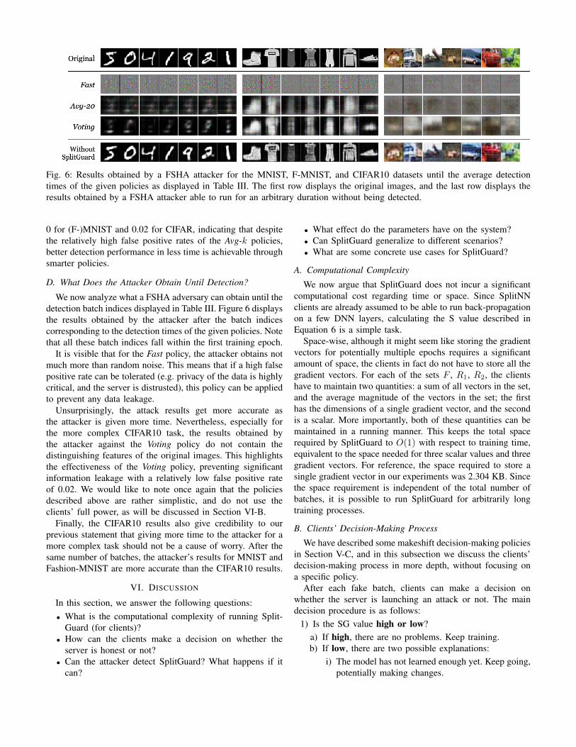
Fig. 6: Results obtained by a FSHA attacker for the MNIST, F-MNIST, and CIFAR10 datasets until the average detectiontimes of the given policies as displayed in Table III. The first row displays the original images, and the last row displays theresults obtained by a FSHA attacker able to run for an arbitrary duration without being detected.

0 for (F-)MNIST and 0.02 for CIFAR, indicating that despitethe relatively high false positive rates of the Avg-k policies,better detection performance in less time is achievable throughsmarter policies.

D. What Does the Attacker Obtain Until Detection?

We now analyze what a FSHA adversary can obtain until thedetection batch indices displayed in Table III. Figure 6 displaysthe results obtained by the attacker after the batch indicescorresponding to the detection times of the given policies. Notethat all these batch indices fall within the first training epoch.

It is visible that for the Fast policy, the attacker obtains notmuch more than random noise. This means that if a high falsepositive rate can be tolerated (e.g. privacy of the data is highlycritical, and the server is distrusted), this policy can be appliedto prevent any data leakage.

Unsurprisingly, the attack results get more accurate asthe attacker is given more time. Nevertheless, especially forthe more complex CIFAR10 task, the results obtained bythe attacker against the Voting policy do not contain thedistinguishing features of the original images. This highlightsthe effectiveness of the Voting policy, preventing significantinformation leakage with a relatively low false positive rateof 0.02. We would like to note once again that the policiesdescribed above are rather simplistic, and do not use theclients’ full power, as will be discussed in Section VI-B.

Finally, the CIFAR10 results also give credibility to ourprevious statement that giving more time to the attacker for amore complex task should not be a cause of worry. After thesame number of batches, the attacker’s results for MNIST andFashion-MNIST are more accurate than the CIFAR10 results.

VI. DISCUSSION

In this section, we answer the following questions:• What is the computational complexity of running Split-

Guard (for clients)?• How can the clients make a decision on whether the

server is honest or not?• Can the attacker detect SplitGuard? What happens if it

can?

• What effect do the parameters have on the system?• Can SplitGuard generalize to different scenarios?• What are some concrete use cases for SplitGuard?

A. Computational Complexity

We now argue that SplitGuard does not incur a significantcomputational cost regarding time or space. Since SplitNNclients are already assumed to be able to run back-propagationon a few DNN layers, calculating the S value described inEquation 6 is a simple task.

Space-wise, although it might seem like storing the gradientvectors for potentially multiple epochs requires a significantamount of space, the clients in fact do not have to store all thegradient vectors. For each of the sets F , R1, R2, the clientshave to maintain two quantities: a sum of all vectors in the set,and the average magnitude of the vectors in the set; the firsthas the dimensions of a single gradient vector, and the secondis a scalar. More importantly, both of these quantities can bemaintained in a running manner. This keeps the total spacerequired by SplitGuard to O(1) with respect to training time,equivalent to the space needed for three scalar values and threegradient vectors. For reference, the space required to store asingle gradient vector in our experiments was 2.304 KB. Sincethe space requirement is independent of the total number ofbatches, it is possible to run SplitGuard for arbitrarily longtraining processes.

B. Clients’ Decision-Making Process

We have described some makeshift decision-making policiesin Section V-C, and in this subsection we discuss the clients’decision-making process in more depth, without focusing ona specific policy.

After each fake batch, clients can make a decision onwhether the server is launching an attack or not. The maindecision procedure is as follows:

1) Is the SG value high or low?a) If high, there are no problems. Keep training.b) If low, there are two possible explanations:

i) The model has not learned enough yet. Keep going,potentially making changes.

ii) The server is launching an attack. Halt training.Going back to the policies we have described in Section V-C,it can be seen that they did not consider the first explanation(1.b.i) of low scores, namely the model not having learnedenough. As we will see, taking that into consideration couldhelp reduce the false positive rates.

The outline contains two branching points: separating highand low scores, and explaining low scores.

Separating High and Low Scores. The process of sepa-rating high and low SplitGuard scores consists of two steps:setting the hyperparameters of the squashing function, anddeciding on a threshold value in the interval (0, 1). Weconsider two scenarios: the clients know or do not know theserver model architecture.

If the clients know the architecture, then the clients can trainthe entire model using all or part of their local data, and gaina prior understanding of what S values (Equation 6) valuesto expect during honest training. The parameters α and β canthen be adjusted to map these values very close to 1. In thisscenario, since the clients’ confidence on the accuracy of themethod is expected to be higher, a relatively high thresholdcan be set, such as 0.95.

If the clients do not know the model architecture, then theyshould set the parameters α and β manually. Nevertheless, Svalues all lying within the interval [−π, π] makes the clients’job easier. It is unreasonable to set extremely high α orβ values since they will cause the squashing function tomake sudden jumps, or map no value close to one. As ourexperiments also demonstrate, smaller values such as 5 and 2are reasonable starting points.

Finally, note that the clients do not have to decide based ona single SplitGuard score. They can consider the entire historyof the score, as depicted in Figure 5 and done in the Avg-kand Voting policies. For example, the score making a suddenjump to 1 and shortly going down to 0.5 does not imply honesttraining; similarly, the score making a sudden jump down to0.5 after consistently remaining close to 1 does not strictlyimply training-hijacking.

Explaining Low Scores. When a client decides that theSplitGuard score is low, it should choose between two possibleexplanations: either the model has not learned enough yet, orthe server is launching a training-hijacking attack.

Informally, a low score indicates that fake gradients arenot that different from regular gradients; the model behavessimilarly when given fake batches and regular batches. In thedomain of classification, behaving similarly is equivalent tohaving a similar classification accuracy. Then, the explanationthat the model has not learned enough yet is more likely ifthe expected classification accuracy for a fake batch is close tothe actual (expected) prediction accuracy. If these values aredifferent but the SplitGuard score is still low, then the serveris very likely launching an attack.

We can formulate the expected accuracy for a fake batch.Say the total number of labels is L ∈ N (L ≥ 2) and theoverall model has classification accuracy A ∈ [1/L, 1]. Then

Fig. 7: Expected classification accuracy in a fake batch withthe share BF of the labels randomized. The model normallyhas classification accuracy A with L labels.

the expected classification accuracy for a fake batch with theshare BF ∈ [0, 1] of the labels randomized is

AF = A · (1−BF ) +BF · (1−A)

L. (7)

Figure 7 explains this equation visually.If the model terminates on the client-side (as in Figure 1b),

then the clients already know the exact accuracy value. If thatis not the case but the clients know the model architectureon the server side, then they can train the model using theirlocal data, and obtain an estimate of the expected classificationaccuracy of the actual model during the first epoch. If eventhat is not possible, then in the worst-case the clients can traina linear classifier appended to their model to obtain a lowerbound on the original model accuracy.7

Formalizing this discussion, for SplitGuard to be effective,it must be the case that A >> AF . If AF ≈ A, then theclients’ choice of BF is not right, and they should increase it.Note that AF is a linear function of BF with the coefficient

−A+1

L− A

L.

Since A ∈ [1/L, 1],

−A+1

L≤ 0

and−A+

1

L− A

L≤ 0

as well. Thus, AF is indeed a monotonic function of BF ,and increasing BF either keeps AF constant or decreases it.Then when the clients decide that the SG value is low and thatAF ≈ A, the best course of action is to increase BF . If BFis already 1, then clients should wait until the model becomessufficiently accurate so that a completely randomized batchmakes a difference. Note that as discussed previously, this isnot a worrisome scenario, since the attack’s effectiveness alsorelies on the model’s adeptness.

7A related, interesting study concludes that what a neural network learnsduring its initial epoch of training can be explained by a linear classifier [22],in the sense that if we know the linear model’s output, then knowing themain model’s output provides almost no benefit in predicting the label. Notehowever that this does not hold for any linear classifier, but the optimal one.

Algorithm 3: Clients’ decision-making processA: Model’s classification accuracyAF : Expected classification accuracy for a fake batchBF : Share of randomized labels in a fake batchN : Number of initial batches to ignoreFunction MAKE_DECISION(F,R):

if scores are high thenKeep training.

else if A ≈ AF thenif BF = 1 then

It is too early to detect. Wait.else

Increase BF .[Optional] Increase N .

elseThe server is launching an attack. Stop training.

Finally, an alternative course of action is to increase N ,discarding the initial group of gradients. Since the modelsbehave randomly in the beginning, increasing N decreasesthe noise, and can help distinguish an honest server from amalicious one. Also note that increasing N is a reversibleprocess, provided that clients store the gradient values.

With these discussions, we can finalize the clients’ decision-making process as the function MAKE_DECISION, displayedin Algorithm 3.

C. Detection by the Attacker

An attacker can in turn try to detect that a client is runningSplitGuard. It can then try to circumvent SplitGuard by usinga legitimate surrogate model as described before.

If the server controls the model’s output (Figure 1a), then itcan detect if the classification error of a batch is significantlyhigher than the other ones. Since SplitGuard is a potential,though not the only, explanation of such behavior, it presentsan opportunity for an attacker to detect it. However, the modelbehaving significantly differently for fake and regular batchesalso implies that the model is at a stage at which SplitGuardis effective. This leads to an interesting scenario: since theattack’s and SplitGuard’s effectiveness both depends on themodel learning enough it seems as if the attack cannot bedetected without the attacker detecting SplitGuard and viceversa.

We argue that this is not the case, due to the clients beingin charge of setting the BF value. For example, with theMNIST dataset for which the model obtains a classificationaccuracy around 98% after the first epoch of training, a BFvalue of 4/64 results in an expected classification accuracy of91.8% for fake batches (Equation 7). The SplitGuard scores onthe other hand displayed in Figure 5 being very close to oneimplies that an attack can be detected with such a BF value.Thus, clients can make it difficult for an attacker to detectSplitGuard by setting the BF value more smartly, rather thansetting it blindly as 1 for better effectiveness.

Finally, we strongly recommend once again that a secureSplitNN setup follow the three-part setup shown in Figure 1bto prevent the clients sharing their labels with the server. Thisway, an attacker would not be able to see the accuracy ofthe model, and it would become significantly harder for it todetect SplitGuard.

D. Choosing Parameter Values

We have touched upon how the clients can decide on BF ,α, and β values, but we need to clarify the effects of theparameter values (mainly BF , PF , and N ) for completeness.Each parameter involves a different trade-off:• Probability of sending a fake batch (PF ).

– (+) Higher PF values mean more fake batches, andthus a more representative sample of fake gradientvalues, increasing the effectiveness of the method.

– (−) Higher PF values can also degrade model perfor-mance, since the server model will be learning randomlabels for a higher number of examples, and a highershare of the potentially scarce dataset will be allocatedfor SplitGuard.

• Number of randomized labels in each batch (BF ).– (+) More random labels in a batch means that fake

batches and regular batches behave even more differ-ently, and the method becomes more effective.

– (−) Depending on the model’s training performance,batches with entirely random labels can be detectedby the server. One way to overcome this difficulty isto perform the loss computation on the client side.

• Number of initial batches to ignore (N ).– (+) A smaller N value means that the server’s mali-

cious behavior can be detected earlier, giving it lesstime to attack.

– (−) Since a model behaves randomly in the beginningof the training, the initial batches are of little value forour purposes. Computing SG scores for later batcheswill make it easier to distinguish honest behavior, butin return give the attacker more time.

E. Generalizing SplitGuard

In the form we have discussed so far, a question might ariseregarding SplitGuard’s effectiveness in different scenarios. Weargue however that since the claims underlying SplitGuardare applicable to any kind of neural network learning onany kind of data, SplitGuard is generalizable to different datamodalities, or more complex architectures. The only caveat, asdiscussed earlier, is that learning on a more complex datasetor with a more complex architecture would require more timefor SplitGuard to be effective.

Another direction of generalization is towards differentattacks. Although there are no training-hijacking attacks otherthan FSHA against which we can test SplitGuard, we claimthat SplitGuard can generalize to future attacks as well. Afterall, SplitGuard relies only on the assumption that randomizingthe labels affects an honest model more than it affects a

malicious model. Thus, to go undetected by SplitGuard, anattack should either involve learning significant informationabout the original task, which would likely reduce the attack’seffectiveness, or craft a different loss function for each label,which could easily be prevented by not sharing the labels withthe server (Figure 1b).

Finally, SplitGuard also generalizes to multiple-clientSplitNN settings. Each client can independently run Split-Guard, with their own choices of parameters. Each clientwould then be making a decision regarding its own trainingprocess. Alternatively, if the clients trust each other, they canchoose one client to run SplitGuard in order to minimize itseffect on performance loss, or they can combine their collectedgradient values and reach a collective decision.8 The latterscenario would be equivalent to a single client training withthe aggregated data of all the clients.

F. Use Cases

We now describe three potential real-world use cases forSplitGuard, modeling clients with different capabilities at eachscenario.

Powerful Clients. A group of healthcare providers decideto train a DNN using their aggregate data while maintainingdata privacy. They decide on a training setup, and establish acentral server.9 Each client knows the model architecture andthe hyperparameters, and preferably has access to the model’soutput as well (no label-sharing). The clients can train modelsusing their local data to determine the parameters α and β.Each client can then run SplitGuard during their training turnsand see if they are being attacked. This is an example scenariowith the clients as powerful as possible, and thus representsthe optimal scenario for running SplitGuard.

Intermediate Clients. The SplitNN server is a researcher,attempting to perform privacy-preserving machine learningon some private dataset of some data-holder (the client).The researcher designs the training procedure, but the data-holder actively takes part in the protocol. The data-holder thushas tight control over how its data is organized. The clientcannot train a local model since it does not know the entirearchitecture, and should set the parameters α and β manually.Nevertheless, it can easily run SplitGuard by modifying thetraining data being used in the protocol.

Weak Clients. An application developer is the SplitNNserver, and the users’ mobile devices are the clients withprivate data. The clients do not know the model architecture,and cannot manipulate how their data is shared with the server.The application developer is in control of the entire processfrom design to execution. In this scenario, SplitGuard shouldbe implemented at a lower-level, such as the ML librariesthe mobile OS supports. However, even in that scenario,the application developer can implement a machine learning

8This is similar to the Voting policy described earlier, where the separationof scores into groups follows naturally from their distributions among theclients.

9Alternatively, members of the group can take turns acting as the SplitNNserver in a P2P manner.

pipeline from scratch, without relying on any libraries. This isnot an optimal scenario for running SplitGuard. There wouldhave to be strict regulations, as well as gatekeeping by theOS provider (e.g. mandating that machine learning code mustuse one of the specified libraries) before SplitGuard couldeffectively be implemented for such clients.

VII. FUTURE DIRECTIONS

We outline three possible avenues of future work relatedto SplitGuard: providing practical implementations, improvingits robustness against detection by the attacker, and developingpotentially undetectable attacks.

Although we provide a proof-of-concept implementationof SplitGuard, it should be readily supported by privacy-preserving machine learning libraries, such as PySyft [23].That way, SplitGuard can be seamlessly integrated into theclient-side processes of split learning pipelines.

As we have explained in Section VI-C, SplitGuard canpotentially, although unlikely, be detected by the attacker,who can then start sending fake gradients from its legitimatesurrogate model and regular gradients from its maliciousmodel. This could again cause a significant difference betweenthe fake and regular gradients, and result in a high SplitGuardscore. However, a potential weakness of this approach bythe attacker is that now the fake gradients result from twodifferent models with different objectives. Suppose the attackerdetects SplitGuard at the 200th batch, and starts using itslegitimate model. Then the fake gradients within the first 200batches will be computed using a malicious model, and thoseafter the 200th batch will be computed using the legitimatemodel. Clients can potentially detect this switch in models,and gain the upper hand. This is another point for which futureimprovement might be possible.

Finally, turning the tables, it might be possible to modifythe existing attacks, or propose novel attacks to produce highSplitGuard scores, very likely at the cost of effectiveness. Thisrepresents another line of future work concerning SplitGuard.

VIII. CONCLUSION

In this paper, we presented SplitGuard, a method forSplitNN clients to detect if they are being targeted by atraining-hijacking attack [11] or not. We described the the-oretical foundations underlying SplitGuard, experimentallyevaluated its effectiveness, and discussed at depth many issuesrelated to its use. We conclude that when used appropriately,and in a secure setting without label-sharing, a client runningSplitGuard can successfully detect training-hijacking attacksand leave the attacker empty-handed.

REFERENCES

[1] T. B. Brown, B. Mann, N. Ryder, M. Subbiah, J. Kaplan, P. Dhari-wal, A. Neelakantan, P. Shyam, G. Sastry, A. Askell, S. Agarwal,A. Herbert-Voss, G. Krueger, T. Henighan, R. Child, A. Ramesh, D. M.Ziegler, J. Wu, C. Winter, C. Hesse, M. Chen, E. Sigler, M. Litwin,S. Gray, B. Chess, J. Clark, C. Berner, S. McCandlish, A. Radford,I. Sutskever, and D. Amodei, “Language Models are Few-Shot Learn-ers,” arXiv:2005.14165 [cs], July 2020. arXiv: 2005.14165.

[2] A. Halevy, P. Norvig, and F. Pereira, “The Unreasonable Effectivenessof Data,” IEEE Intelligent Systems, vol. 24, pp. 8–12, Mar. 2009.

[3] N. C. Thompson, K. Greenewald, K. Lee, and G. F. Manso, “The com-putational limits of deep learning,” arXiv preprint arXiv:2007.05558,2020.

[4] G. J. Annas, “HIPAA Regulations — A New Era of Medical-RecordPrivacy?,” New England Journal of Medicine, vol. 348, pp. 1486–1490,Apr. 2003.

[5] R. T. Mercuri, “The HIPAA-potamus in health care data security,”Communications of the ACM, vol. 47, pp. 25–28, July 2004.

[6] P. Vepakomma, O. Gupta, T. Swedish, and R. Raskar, “Split learningfor health: Distributed deep learning without sharing raw patient data,”arXiv preprint arXiv:1812.00564, 2018.

[7] O. Gupta and R. Raskar, “Distributed learning of deep neural networkover multiple agents,” arXiv:1810.06060 [cs, stat], Oct. 2018. arXiv:1810.06060.

[8] K. Bonawitz, H. Eichner, W. Grieskamp, D. Huba, A. Ingerman,V. Ivanov, C. Kiddon, J. Konecny, S. Mazzocchi, H. B. McMahan,T. Van Overveldt, D. Petrou, D. Ramage, and J. Roselander, “TowardsFederated Learning at Scale: System Design,” arXiv:1902.01046 [cs,stat], Mar. 2019. arXiv: 1902.01046.

[9] J. Konecny, H. B. McMahan, D. Ramage, and P. Richtarik, “FederatedOptimization: Distributed Machine Learning for On-Device Intelli-gence,” arXiv:1610.02527 [cs], Oct. 2016. arXiv: 1610.02527.

[10] J. Konecny, H. B. McMahan, F. X. Yu, P. Richtarik, A. T. Suresh, andD. Bacon, “Federated Learning: Strategies for Improving Communica-tion Efficiency,” arXiv:1610.05492 [cs], Oct. 2017. arXiv: 1610.05492.

[11] D. Pasquini, G. Ateniese, and M. Bernaschi, “Unleashing the Tiger:Inference Attacks on Split Learning,” arXiv:2012.02670 [cs], Jan. 2021.

[12] Y. LeCun, C. Cortes, and C. Burges, “Mnist handwritten digit database,”ATT Labs [Online]. Available: http://yann.lecun.com/exdb/mnist, vol. 2,2010.

[13] H. Xiao, K. Rasul, and R. Vollgraf, “Fashion-mnist: a novel imagedataset for benchmarking machine learning algorithms,” arXiv preprintarXiv:1708.07747, 2017.

[14] A. Krizhevsky, G. Hinton, et al., “Learning multiple layers of featuresfrom tiny images,” 2009.

[15] I. Goodfellow, Y. Bengio, and A. Courville, Deep Learning. MIT Press,2016. http://www.deeplearningbook.org.

[16] S. Ruder, “An overview of gradient descent optimization algorithms,”arXiv:1609.04747 [cs], June 2017. arXiv: 1609.04747.

[17] P. Vepakomma, T. Swedish, R. Raskar, O. Gupta, and A. Dubey, “Nopeek: A survey of private distributed deep learning,” arXiv preprintarXiv:1812.03288, 2018.

[18] A. Singh, P. Vepakomma, O. Gupta, and R. Raskar, “Detailed com-parison of communication efficiency of split learning and federatedlearning,” arXiv preprint arXiv:1909.09145, 2019.

[19] K. He, X. Zhang, S. Ren, and J. Sun, “Deep residual learning for imagerecognition,” in Proceedings of the IEEE conference on computer visionand pattern recognition, pp. 770–778, 2016.

[20] D. P. Kingma and J. Ba, “Adam: A Method for Stochastic Optimization,”arXiv:1412.6980 [cs], Jan. 2017. arXiv: 1412.6980.

[21] A. Paszke, S. Gross, F. Massa, A. Lerer, J. Bradbury, G. Chanan,T. Killeen, Z. Lin, N. Gimelshein, L. Antiga, A. Desmaison, A. Kopf,E. Yang, Z. DeVito, M. Raison, A. Tejani, S. Chilamkurthy, B. Steiner,L. Fang, J. Bai, and S. Chintala, “Pytorch: An imperative style, high-performance deep learning library,” in Advances in Neural InformationProcessing Systems 32 (H. Wallach, H. Larochelle, A. Beygelzimer,F. d'Alche-Buc, E. Fox, and R. Garnett, eds.), pp. 8024–8035, CurranAssociates, Inc., 2019.

[22] D. Kalimeris, G. Kaplun, P. Nakkiran, B. Edelman, T. Yang, B. Barak,and H. Zhang, “Sgd on neural networks learns functions of increas-ing complexity,” Advances in Neural Information Processing Systems,vol. 32, pp. 3496–3506, 2019.

[23] T. Ryffel, A. Trask, M. Dahl, B. Wagner, J. Mancuso, D. Rueckert, andJ. Passerat-Palmbach, “A generic framework for privacy preserving deeplearning,” arXiv preprint arXiv:1811.04017, 2018.