spin dynamics and structural modifications of co2mnsi
TRANSCRIPT

HAL Id: tel-02073985https://tel.archives-ouvertes.fr/tel-02073985v3
Submitted on 16 Dec 2016
HAL is a multi-disciplinary open accessarchive for the deposit and dissemination of sci-entific research documents, whether they are pub-lished or not. The documents may come fromteaching and research institutions in France orabroad, or from public or private research centers.
L’archive ouverte pluridisciplinaire HAL, estdestinée au dépôt et à la diffusion de documentsscientifiques de niveau recherche, publiés ou non,émanant des établissements d’enseignement et derecherche français ou étrangers, des laboratoirespublics ou privés.
Spin dynamics and structural modifications of Co2MnSiHeusler alloys by helium ions irradiation
Iman Abdallah
To cite this version:Iman Abdallah. Spin dynamics and structural modifications of Co2MnSi Heusler alloys by heliumions irradiation. Physics [physics]. Université Paul Sabatier - Toulouse III, 2016. English. NNT :2016TOU30079. tel-02073985v3

et discipline ou spécialité
Jury :
le
Université Toulouse 3 Paul Sabatier (UT3 Paul Sabatier)
Iman ABDALLAH
lundi 23 mai 2016
Spin dynamics and structural modifications of Co2MnSi Heusler alloys by
Helium ions irradiation
ED SDM : Physique - COR 02
CEMES-CNRS
Philippe LECOEUR Rapporteur IEF Orsay
Matthieu BAILLEUL Rapporteur IPCMS Strasbourg
Marc RESPAUD Examinateur LPCNO-INSA Toulouse
Pascale BAYLE-GUILLEMAUD Examinatrice INAC-CEA Grenoble
Gérard BENASSAYAG Invité CEMES-CNRS Toulouse
Nicolas BIZIERE
Etienne SNOECK


Acknowledgments
Here comes the moment to thank the people who devoted their time and knowledge for this
work to be completed and published. After tremendous hard work and continues effort, this
is the fruit of the three past years. I am thankful to my thesis directors Nicolas BIZEIRE and
Etienne SNOECK for endorsing me to achieve this work.
First I thank the members of the jury for reviewing and commenting on my manuscript
and giving me this opportunity to publish this work. I want to thank the rapporteurs Dr.
Philippe LECOUER from IEF in Orsay and Dr. Matthieu BAILLEUL from IPCMS in
Strasbourg for their comments and positive evaluations. I thank as well Dr. Marc RESPAUD,
the president of the jury, from INSA in Toulouse and Dr. Pascale BAYLE-GAUILLEMAUD
from INAC-CEA in Grenoble for their fruitful comments on the manuscript.
I want to express my gratitude to my advisor Nicolas Biziere for his continues support,
coordination and friendly encouragement during the past three years to achieve this work.
Thank you for offering me this opportunity to work on this diverse subject. Thank you for
putting me on the right tracks and for all the professional and social discussions we had. I
thank as well Etienne Snoeck for his coordination and immense help in the microscopy part.
I want as well to thank many researchers whom without this work wasn’t possible to
be completed. Thank you Gerard BENASSAYAG for all the discussions, simulations and
massive help in the ion irradiation part. Thank you for being a part of this work. I thank a
well Beatrice PECASSOU for the ion irradiation experiments. I would like also to thank Jean-
Francois BOBO for his mentoring and guidance to use the sputtering machine. I want to
thank Nicolas RATEL-RAMOND and Alexandre ARNOULT for X-ray Diffraction
experiments and their tremendous help to achieve the results we wanted. I last want to thank
both César Magen from for the STEM experiments at LMA-INA, Zaragoza-Spain and my
friend Luis Alfredo RODRIGUEZ for the Lorentz microscopy experiments done at CEMES.
Family and friends, without your support and courage during the whole period of stay
in France from the beginning of the journey in Strasbourg to its end in Toulouse, I couldn’t
make it without you. From a personal perspective, I need to thank the people who I am with
became a better person. My parents, Sobhi and Zeinab, I am grateful for what you have raised
me to become a better person in this world no matter what difficulties someone may encounter
in life. My two brothers Salam and Ali and their lovely families, my lovely sister Ahlam and
her family, thank you for all the encouragement and support throughout the years. Ahmad,
Mariam, Hadi and Karam, this thesis is dedicated for you my beloved ones.

Special thanks go to my friends from CEMES and IPCMS in Strasbourg. Thank you
for the support and for being a part in my life. I want to thank in person, Fatima Ibrahim, Ali
HALLAL, Mohammad HAIDAR, Ferdaous BEN ROMDHANE, Ahmed MAGHRAOUI,
Wasim JABER, Rania NOUREDDINE, Batoul SROUR, Imane Malass, Luis Alfredo
RODREGEUZ, David REYES, Thibaud DENNEULIN, Marion CASTIELA, XIAOXIAO FU
and all my friends and colleagues I have met. At the end I wish all the luck to Ines ABID,
Barthelemy PRADINS and Thomas GARANDEL in their last year of PhD.
Iman ABDALLAH,
Toulouse, the 23rd of May 2016.
1
Table of contents
Introduction .............................................................................................................................. 4
Chapter 1: Heusler alloys State of the Art .......................................................................... 7
1.1 Crystalline structure of Co-based Heusler alloys ........................................................ 8
1.2 Half-metallic behavior ................................................................................................. 10
1.3 Magnetic behavior ....................................................................................................... 12
1.3.1 Origin of magnetism in Heusler alloys ................................................................... 12
1.3.2 Curie temperature ................................................................................................... 14
1.4 Several effects on half-metallicity and magnetic behavior of Heusler alloys. ......... 15
1.4.1 Effect of atomic disorder .......................................................................................... 15
1.4.2 Effect of surface and interface ................................................................................. 16
1.5 Ion irradiation/implantation ....................................................................................... 18
1.6 Applications of Heusler alloys .................................................................................... 19
1.7 Choice of Co2MnSi Heusler compound ....................................................................... 20
1.7.1 Saturation Magnetization ....................................................................................... 20
1.7.2 Magneto-crystalline anisotropy constant ............................................................... 21
1.7.3 Exchange constant ................................................................................................... 21
1.7.4 Magnetic damping factor ......................................................................................... 21
Chapter 1 References: ............................................................................................................ 23
Chapter 2: Magnetization Dynamics ................................................................................. 29
2.1 Basics of Magnetism .................................................................................................... 29
2.2 Micro-magnetic energy terms of ferromagnetic thin films ........................................ 32
2.2.1 Zeeman Energy ........................................................................................................ 32
2.2.2 Exchange energy ...................................................................................................... 32
2.2.3 Demagnetization energy .......................................................................................... 34
2.2.4 magneto-crystalline Anisotropy energy .................................................................. 34
2.3 Magnetization dynamics ............................................................................................. 37
2.3.1 Equation of motion LLG and its solution ............................................................... 37
2.3.2 Ferromagnetic resonance in thin films ................................................................... 41
2.4 Spin waves ................................................................................................................... 44
2.4.1 Magnetostatic regime .............................................................................................. 45
2.4.1.1 Magnetostatic modes ........................................................................................ 45
2.4.2 Spin waves in the exchange regime ........................................................................ 49
2.4.2.1 Standing Spin waves (SSW) ............................................................................. 50
2.5 Magnetization relaxation mechanism ........................................................................ 51
2.5.1 Intrinsic relaxation processes ................................................................................. 52
2.5.2 Extrinsic relaxation processes ................................................................................. 55
Chapter 2 References: ............................................................................................................ 58

2 Table of contents
Chapter 3: Experimental techniques ................................................................................. 61
3.1 Deposition Techniques ................................................................................................ 61
3.1.1 Sputtering ................................................................................................................ 62
3.1.1.1 Presentation of PLASSYS sputtering chamber .............................................. 64
3.2 CMS Thin film deposition procedure .......................................................................... 65
3.3 Structural characterization techniques ..................................................................... 66
3.3.1 Basics of crystallography diffraction ...................................................................... 67
3.3.2 Reflection High Energy Electron Diffraction (RHEED) ........................................ 68
3.3.3 X-ray Diffraction (XRD) ........................................................................................... 69
3.3.4 Transmission Electron Microscopy (TEM) ............................................................. 72
3.3.4.1 High Resolution Electron Microscopy (HRTEM): ........................................... 75
3.3.4.2 Scanning Transmission Electron Microscopy (STEM): .................................. 77
3.3.4.3 Geometric Phase Analysis (GPA): .................................................................... 78
3.3.4.4 Lorentz Microscopy (LM): ................................................................................. 79
3.4 Magnetic characterization techniques ....................................................................... 84
3.4.1 Physical Property Measurement System (PPMS) .................................................. 84
3.4.2 Magneto-Optical Kerr Effect (MOKE) .................................................................... 84
3.4.3 Ferromagnetic Resonance (FMR)............................................................................ 86
3.4.3.1 FMR Experimental set-up ................................................................................ 87
3.5 Ion irradiation/implantation technique ...................................................................... 91
3.5.1 Ion-Solid interaction ................................................................................................ 92
Chapter 3 References: ............................................................................................................ 93
Chapter 4: Structural and magnetic properties of as deposited CMS samples ....... 95
4.1 Structural properties of CMS samples ....................................................................... 96
4.1.1 Determination of deposition conditions .................................................................. 96
4.1.2 Atomic disorder by X-ray Diffraction ...................................................................... 98
4.1.3 Structural investigation by HRTEM and HAADF-STEM ................................... 107
4.2 Magnetic properties ................................................................................................... 114
4.2.1 MOKE measurements: switching field mechanisms ........................................... 114
4.2.2 Domain walls observation by Lorentz microscopy ............................................... 124
4.2.3 FMR Dynamic properties measurements ............................................................. 125 4.2.3.1 Extraction of magnetic parameters. ........................................................................................ 126 4.2.3.2 Study of dynamic relaxation: anisotropic damping ................................................................. 138
4.3 Conclusion .................................................................................................................. 146
Chapter 4 References: .......................................................................................................... 148
Chapter 5: Effect of He+ ions irradiation on structural and magnetic properties of
CMS Heusler alloys .............................................................................................................. 150
5.1 Irradiation with Helium ions (He+) at 150 keV ....................................................... 151
5.1.1 Simulation of Co2MnSi irradiation with He+ ions ................................................ 151

3
5.2 Induced atomic disorder by X-ray diffraction and STEM ....................................... 153
5.3 Modifications of magnetic properties by He+ ions irradiation ................................ 161
5.3.1 Static magnetic properties .................................................................................... 161
5.3.2 FMR measurements of irradiated samples: effect of irradiation on magnetic
parameters ........................................................................................................................ 163
5.3.3 Effect of He+ irradiation on the Gilbert Damping ................................................ 176
Chapter 5 References: .......................................................................................................... 187
Conclusion and Perspective .............................................................................................. 189
4 Introduction
Introduction
Spintronic, which involve electron’s spin for data storage and processing, has emerged
from the discovery of Giant magnetoresistance (GMR) by A. Fert and P. Grunberg in 1988 [1
Baibich, 2 Binasch] few years after the prediction of Tunneling magnetoresistance (TMR) by
M. Julliere in 1975 [3 Julliere, 4 Miyazaki, 5 Moodera]. This discovery, rewarded by a Nobel
Prize in 2007, has revolutionized the field of sensor devices, allowing for very weak magnetic
field detection. The highest TMR reached today at room temperature is 604% by suppression
of Ta diffusion on CoFeB/MgO/CoFeB [6 Ikeda]. Among the numerous applications of
magneto-resistive effects, one of the most famous is the development of Magnetic Random
Access Memories (MRAM) for data storage and processing, developed in the 2000’s. Another
very active topic in spintronics deals with the spin transfer torque (STT) effect [7 Slonczewski,
8 Berger] which relates the effect of a spin polarized current upon the magnetization of a
nanostructure. Indeed, for sufficiently high current density, one can switch the magnetization
of a nanomagnet or induce its precession in the GHz or THz range. Similarly to magneto-
resistive effects, STT is now the basis of numbers of devices such as ST-MRAM or microwave
devices.
The basic mechanism of GMR and TMR relies on the spin polarization, i.e. the
difference between majority and minority spins at the fermi level, of the material. STT effect
also depends on spin polarization but also on the dynamic damping coefficient which opposes
the STT. Indeed, the current density to switch the magnetization of a nanomagnet is
proportional to the Gilbert damping constant and inversely proportional to the spin
polarization. Therefore there is today an intense research to find materials with both high
spin polarization and low damping coefficient. In this research field, one promising route
concerns Heusler alloys which are predicted to be half metals, meaning theoretically 100%
spin polarization, with a weak Gilbert damping coefficient below 10-3, about one order of
magnitude below the usual ferromagnetic material used in microelectronic.
After the discovery of Heusler alloys by F. Heusler [9 Heusler], half metallicity proof
of NiMnSb half-Heusler compound was reported by de Groot et al. [10 de Groot] leading to a
great interest in investigating different kinds of Heusler alloys. Nowadays, the improvement
of structural and magnetic properties of Heusler alloys has become a major topic in
spintronics.
In this work we offer to study the correlations between the structural and magnetic
properties of the particular Co2MnSi Heusler alloy. The interests for this material are
multiple. First it is predicted to be half metallic when ordered in the L21 or B2 crystal phases.
Also, it has been predicted to show very low damping coefficient down to 6x10⁻⁴ which is about
one order of magnitude lower than the usual ferromagnetic materials. Its high Curie
temperature up to 800° K provides stability for devices working at room temperature. Last,
the deposition conditions of this alloy are compatible with microelectronics processes.
Therefore it shows multiple advantages for the development of new generation of spintronic
devices.
To achieve our goal, we study the evolution of the static and dynamic magnetic
parameters of the Co2MnSi when submitted to He+ ion irradiation at 150 KeV. Ion irradiation
is a particular efficient method to control and/or modify the structure of magnetic alloys. For

5
example, the improvement of long range L10 order of FePt and FePd alloys was demonstrated
by ion irradiation in the early 2000’s. More recently, Gaier et al. [11 Gaier] showed in 2009
that He+ ion irradiation improves the long range B2 order in Co2MnSi. Our work is an
extension of the one of Gaier. Our initial objectives are twofold. The first is to study the
possibility to use ion irradiation to enhance the structural order and magnetic properties of
the Co2MnSi, even in the most ordered L21 phase, and to decrease the microwave losses in
the Gigahertz range. The second objective is more fundamental as it consists in studying the
intrinsic and extrinsic contributions of the dynamic relaxation as a function of the atomic
order. Our goal is to get a better understanding of the intrinsic mechanisms controlling the
magnetic dynamic relaxation.
To reach these different objectives, we combined several experimental techniques. We
grow Co2MnSi Heusler alloys by magnetron sputtering on MgO substrates. These samples
are then irradiated with light He+ ions. The structural properties of the samples are studied
by X-ray diffraction, in normal and anomalous conditions, and with Transmission Electron
Microscopy (TEM) techniques, in particular HAADF-STEM imaging mode. This part of our
study has been realized in collaboration with the LAAS-CNRS Laboratory in Toulouse and
with the INA-ARAID laboratory at the University of Zaragoza (Spain). The evolution
of the static and dynamic magnetic properties of the samples has been measured by
means of Magneto Optic Kerr Effect (MOKE), Physical Properties Measurements System
(PPMS) at the LPCNO laboratory in Toulouse and Ferromagnetic Resonance (FMR). The
FMR set-up has been developed at the CEMES during this PhD.
The manuscript is organized as follow:
In chapter 1 we give an overview of the state of the art about full X2YZ Heusler alloys and
in particular the structural and magnetic behavior of Co2MnSi. In this chapter, we also
include some features affecting the half metallicity as well as the magnetic behavior. In
particular a review of the effect of atomic disorder and deposition conditions on the
magnetic properties is addressed.
In chapter 2 we present some basics of magnetism starting with the micromagnetic energy
terms involved in the understanding of the static and magnetic behavior of ferromagnetic
films. Then magnetization dynamics is presented and spin waves concept is introduced.
At the end of this chapter, we introduce the concept of intrinsic and extrinsic dynamic
relaxation mechanisms.
The chapter 3 presents the different experimental techniques that we used in this work
for the deposition of thin films and irradiation processes as well as experimental methods
for structural and magnetic characterization of the thin films.
In chapter 4, we present the structural and magnetic properties of 3 different series of
CMS samples, showing different initial structural and magnetic properties. In this
chapter we address the problem of the determination of the static and magnetic
parameters due to the observed atomic disorder.

6 Introduction
The chapter 5 is devoted to the study of the effect of He+ ion irradiation on the three series
of samples. We will show how the irradiation modifies both the mechanical strain in the
material as well as the chemical arrangement. Then the effect of these structural
modifications on the magnetic properties will be addressed, with a highlight on the
variation of the crystal anisotropy in the samples. In the final part of this chapter,
preliminary results on the effect of atomic disorder on the evolution of the intrinsic and
extrinsic dynamic relaxation parameters will be presented. We will show that the B2 and
L21 orders shows different evolution under irradiation, leading to different behavior of
their magnetic properties.
References:
[1] M. N. Baibich, J. M. Broto, A. Fert, F. N. Van Dau, F. Petroff, P. Etienne, G. Creuzet, A.
Friederich, et J. Chazelas, « Giant magnetoresistance of (001) Fe/(001) Cr magnetic
superlattices », Phys. Rev. Lett., vol. 61, no 21, p. 2472, 1988.
[2] G. Binasch, P. Grünberg, F. Saurenbach, et W. Zinn, « Enhanced magnetoresistance in
layered magnetic structures with antiferromagnetic interlayer exchange », Phys. Rev. B,
vol. 39, no 7, p. 4828, 1989.
[3] M. Julliere, « Tunneling between ferromagnetic films », Phys. Lett. A, vol. 54, no 3, p.
225‑226, sept. 1975.
[4] T. Miyazaki et N. Tezuka, « Giant magnetic tunneling effect in Fe/Al2O3/Fe junction », J.
Magn. Magn. Mater., vol. 139, no 3, p. L231‑L234, janv. 1995.
[5] J. S. Moodera, L. R. Kinder, T. M. Wong, et R. Meservey, « Large magnetoresistance at
room temperature in ferromagnetic thin film tunnel junctions », Phys. Rev. Lett., vol. 74,
no 16, p. 3273, 1995.
[6] S. Ikeda, J. Hayakawa, Y. Ashizawa, Y. M. Lee, K. Miura, H. Hasegawa, M. Tsunoda, F.
Matsukura, et H. Ohno, « Tunnel magnetoresistance of 604% at 300K by suppression of
Ta diffusion in CoFeB∕MgO∕CoFeB pseudo-spin-valves annealed at high temperature »,
Appl. Phys. Lett., vol. 93, no 8, p. 082508, août 2008.
[7] « J. Slonczewski, Journal of Magnetism and Magnetic Materials, vol. 159, page L1
(1996) ».
[8] L. Berger, « A simple theory of spin-wave relaxation in ferromagnetic metals », J. Phys.
Chem. Solids, vol. 38, no 12, p. 1321‑1326, janv. 1977.
[9] F. Heusler, W. Starck, and E. Haupt, Verh. DPG 5, 220 (1903) .
[10] R. A. De Groot, F. M. Mueller, P. G. Van Engen, et K. H. J. Buschow, « New class of
materials: half-metallic ferromagnets », Phys. Rev. Lett., vol. 50, no 25, p. 2024–2027,
1983.
[11] O. Gaier, « A study of exchange interaction, magnetic anisotropies, and ion beam
induced effects in thin films of Co2-based Heusler compounds », Ph. D. dissertation,
Technical University of Kaiserslautern, 2009.

7
Chapter 1: Heusler alloys
State of the Art
In 1903 F. Heusler has discovered a new class of intermetallic materials that exhibit
a ferromagnetic order although none of its constituent elements are magnetic in Cu2MnAl
alloy [1 Heusler]. These alloys are ternary compounds and divided into two categories, Half
Heusler (XYZ) and Full Heusler alloys (X2YZ) where, X, Y are transition metals elements and
Z belong to sp elements group (Table 1.1).
Table 1.1: periodic table of elements showing the different species of Heusler alloys.
Adapted from [2 Graf]
Enormous investigations were conducted to study Heusler alloys for spintronic
applications, in the last two decades, due to two main magnetic properties. The first one is
the half metallic behavior which means that the material behaves as an insulator or a
semiconductor for one spin orientation and as a metal for another orientation. The other
important property, which is of particular interest in this thesis manuscript, is the low Gilbert
damping coefficient that is predicted to be below 10-3. The mentioned properties were first
investigated by ab-intio calculations [3 de Groot]. De Groot et al. have shown the half metallic
behavior in NiMnSb Heusler compounds; this discovery led to a great interest in studying
Heusler alloys. Since then, different atomic combinations have been tested as for example Co-
based Heusler compounds. During the last 10 years, experimental work focused on the growth
quality and the different magnetic properties of Heusler alloys.
The advantages of Heusler alloys are their electronic, magnetic and magneto-optical
properties along with high thermal stability. Half Heusler alloys gained a lot of interest in
the thermoelectric and solar applications [4 Bartholomé]. On the other hand, full Heusler
alloys were specially investigated in spintronic applications. Examples on some applications
of half and full Heusler alloys are given at the end of this chapter. In this work we focus on

8 Chapter 1: Heusler alloys “state of the art”
the magnetic properties and especially the dynamic properties, of Co2MnSi which is predicted
to be half metallic with a very low damping ≈ 0.6 x 10⁻⁴ [5 Liu]. Moreover, its high Curie
temperature (around 980 K) [6 Webster] makes it compatible with micro-electronic processes
and promotes it as a promising candidate for spintronic devices.
In this chapter, we will present the general structural and magnetic properties of
Heusler alloys, with a particular insight on Co-based Heusler compounds. Half metallicity
and magnetic behavior will be presented. Then, we will present the influence of structural
ordering on the magnetic properties and the half metallicity. The discussion about the
damping will be presented in chapter 2. Then, the effect of ion irradiation on the Heusler
alloys properties will be addressed and some examples of industrial applications with half
and full Heusler alloys will be given. Finally, we give a summary of the reported values in
literature for several magnetic parameters of the particular Co2MnSi Heusler alloy which is
the topic of our work.
1.1 Crystalline structure of Co-based Heusler alloys
Full Heusler alloys of general composition Co2YZ preferably crystallize in L21
structure (space group Fm3m). The cubic unit cell is made up of four interpenetrating FCC
sublattices and atoms are placed following Wyckoff positions. Co atoms are placed at (1/4, 1/4,
1/4) position of the unit cell, Y and Z atoms are placed at (0, 0, 0) and (1/2, 1/2, 1/2) respectively,
as shown in (Fig.1.1-a). L21 phase is the most ordered phase of Heusler alloys. If the atoms
are misplaced or occupied randomly in the unit cell, the ordered phase is no longer valid.
Heusler alloys also exist in three other crystalline phases, the partially disorder B2 and D03
phases, and the completely disordered A2 phase. The B2 phase is formed by a random
distribution of the Y and Z atoms positions in the unit cell but keeping Co atoms at their
initial positions (Fig.1.1-b). The interchange of Co and Y atoms in the unit cell results in a
formation of D03 structure (Figure 1.1-c). The completely disordered phase A2 is formed when
all atoms are randomly occupied in the unit cell (Fig.1.1-c) [7 Bacon and Plant, 6 Webster, 8
Trudel]. In our work we focused on the Co2MnSi alloy which preferentially grows in the L21
order. However, it is important to note that it can grow into the chemically disordered B2 and
(A2) structures depending on the deposition conditions.
Figure 1.1: schematic presentation of Co2YZ crystalline structure: a) L21, b) B2, c) D03 and
A2 phases.

9
The stability of L21 crystal order in Heusler alloy depends on the elements occupying
X, Y and Z. Kobayashi et al. showed that the B2/ L21 transition temperature for the Co2YGa
(Y=Ti, V, Cr) alloys monotonically decreases with increasing electron concentration of the Y
site, whereas the transition temperature is almost constant at 1100±100 K for (Y=Mn, Fe) [9
Kobayashi]. This behavior may be related to the interaction between Y atoms and Ga.
Also, Z atoms can affect the ordering structure of Co based Heusler alloys, for example,
Co2MnSi and Co2MnAl tend to crystallize in the L21 and B2 order respectively and this is due
to different bonding energy between Si or Al atoms and the transition metals [10 kandpal].
The nature of the Z atom has also an influence on the lattice parameter of Co based Heusler
alloys. As an example ,table 1.2 presents the different lattice parameters for Co2MnZ alloys
that ranges from 5.6 to 5.7 [6 Webster, 11 Elmers, 12 Wurmehl].
Heusler compounds Lattice parameter a
()
Crystalline
structure
Curie temperature
(K°)
Co2MnSi 5.654
[6 Webster]
L21 985
[6 Webster,13
Brown]
Co2MnAl 5.756
[6 Webster]
B2 693
[6 Webster,14
Bushow]
Co2MnGe 5.743
[6 Webster]
L21 905
[6 Webster, 14
Bushow]
Co2FeAl 5.730
[10 Kandpal]
B2 1000
[14 Bushow]
Co2FeSi 5.640
[12 Wurmel]
L21 1100
[12 Wurmel]
Table 1.2: crystalline structure and lattice parameters of some Co based Heusler alloys.
The structural properties of Co based Heusler alloy are very sensitive to the deposition
condition and especially on the nature of the substrate in order to minimize lattice mismatch
defined as: 𝑎𝑑𝑒𝑝𝑜𝑠𝑖𝑡𝑒𝑑 𝑓𝑖𝑙𝑚−𝑎𝑠𝑢𝑏𝑠𝑡𝑟𝑎𝑡𝑒
𝑎𝑠𝑢𝑏𝑠𝑡𝑟𝑎𝑡𝑒.
In literature, different substrates have been used to grow Co-based Heusler alloys like
Ge (001) [15 Li], n-type Ge (111) [16 Nahid], GaAs and MgO (001). One of the major interest
of using MgO substrate is for Magnetic tunnel junctions (MTJs) applications, while GaAs
substrates allow for spin injection in semiconductor applications. GaAs has a lattice
parameter of 5.65 Å while that of MgO is 4.21 Å (Figure 1.2). This leads to a better lattice
mismatch for GaAs where the Co based Heusler alloys grow cube on cube. For MgO, epitaxial
growth is achieved via a 45° rotation of the CMS axis with respect to MgO <100> direction.
The lattice mismatch of Co2MnSi on MgO is ≈ - 5.1% (Figure 1.2-a).

10 Chapter 1: Heusler alloys “state of the art”
Figure 1.2: schematic presentation of the epitaxial growth of Co2MnSi on a) MgO and b)
GaAs.
Many groups have introduced Cr as a seed layer between the substrate and the
deposited Heusler films [17 Ortiz, 18 Gaier, 8 Trudel]. The use of seed layers [19 Magen] and
a single crystalline substrate [20 Garcia], improves the crystalline quality of the deposited
thin film. For example, with the Cr seed layer, the lattice mismatch between the Cr/MgO and
for Co2MnSi/Cr is reduced to -2.4 % and -2.6 % respectively. Cr deposition is useful to reduce
the strain at the interfaces and therefore enhance the magnetic properties of Co2MnSi
compared to films deposited directly on MgO substrates [17 Ortiz].
In the next section, we provide more details about the effects of surface termination
and interface on the half metallicity and magnetic properties of Co-based Heusler compounds
with a particular focus on Co2MnSi which is the material studied in the framework of this
thesis.
1.2 Half-metallic behavior
As mentioned before, high spin polarization at the Fermi energy is crucial to realize
efficient TMR-based spintronic devices. Half metallic materials match this criteria. Several
materials are known to be half metallic such as Cr oxides, magnetite Fe3O4, manganite
(La0.7Se0.3MnO3) [21 Soulen], the double perovskites (Sr2FeReO6) [22 Kato] and the pyrites
(CoS2) [23 Shishido]. Besides these materials, Heusler alloys attracted a lot of interest for
being half metallic. In this section, origin of band gap and some effects on half metallicity are
discussed.
Half-metallic materials exhibit a unique band structure. For one spin channel they are
metallic while for the other they are semiconductors or insulators due to the gap in the density
of states (DOS) at the Fermi energy level (Figure 1.3). This leads to a 100% spin polarization
𝑷 of the conduction spin channel.
𝑷 =𝐷 ↑ (𝐸𝑓) − 𝐷 ↓ (𝐸𝑓)
𝐷 ↑ (𝐸𝑓) + 𝐷 ↓ (𝐸𝑓)

11
Figure 1.3: schematic presentation of the DOS of half metallic ferromagnetic, P=1 from
electron’s spin polarization at the Fermi level. Adapted from [24]
The half metallic behavior of Heusler alloys were first predicted by spin-dependent
band structure ab-initio calculations of NiMnSb and PtMnSb by de Groot et al. [3 de Groot].
After this discovery, many Co-based Heusler alloys were theoretically predicted to be half-
metallic. As an example, Figure 1.4 shows the total Density of States (DOS) for different
Co2MnZ alloys. It is clearly visible that no states at the fermi level are available for minority
spin except for Z = Ga for which the DOS is not zero at Fermi energy.
Figure 1.4: Spin resolved DOS for Co2MnZ compounds with Z=Al,Ga,Si and Ge. Taken from
[25 Galanakis].
The origin of the band gap for minority spins in these alloys have been studied in
details by Galanakis in 2002 [25 Galanakis]. The starting point is the hybridization between
Co-Co d-states and the Mn d-orbitals. The hybridization between Co-Co d-states is
schematized in Figure 1.5-a leading to bonding (eg, t2g) and antibonding (eu, t1u) orbitals.
Let’s note that this mechanism is strongly dependent on the distance between the two Co
atoms. Then these degenerated orbitals couple with the d states of the Mn atoms (Figure 1.5-
b) to create bonding and antibonding orbitals below and above the fermi level. It is noteworthy
that only minority spins are represented here. However for majority spins, the exchange

12 Chapter 1: Heusler alloys “state of the art”
energy decreases the energy of the majority d spin states of Mn atoms which couple with the
Co d states and avoid the energy gap.
Figure 1.5: schematic presentation of the origin of band gap in Heusler alloys [26
Galanakis]. a) Hybridization between Co-Co atoms and b) with the Mn states. d1, d2 and d3
indicates 𝑑𝑥,𝑦 , 𝑑𝑦𝑥 and 𝑑𝑧𝑥 𝑡2𝑔 orbitals respectively. d4 and d5 stands for 𝑑𝑧2 , 𝑑𝑥2−𝑦2 𝑒𝑔
orbitals. The number in front of the orbitals is the degeneracy of each orbital.
The scenario proposed by Galanakis is now commonly accepted in the Heusler
community. It is, however, interesting to note that in this mechanism the sp-elements are not
responsible for the existence of the minority gap. This is due to the fact that Z atoms introduce
a deep lying s-p-bands below the center of the d-bands [26 Galanakis]. However the sp
element modifies the position of the fermi level by changing the total number of valence
electrons as it has been shown by Galanakis et al. in Co2MnZ alloys with Z being Si, Sn, Ga,
Ge or Al (Figure 1.4).
1.3 Magnetic behavior
1.3.1 Origin of magnetism in Heusler alloys
Half metallic Heusler alloys exhibit an interesting magnetic behavior along with high
curie temperatures. Heusler alloys can be ferromagnetic, ferrimagnetic or antiferromagnetic
[27 Picket, 28 Casper]. However, the majority of Heusler alloys have a ferromagnetic
behavior.
Magnetic properties of Co-based Heusler alloys will be presented with a focus on
magnetic moments, anisotropy field, and exchange interaction constant in Co2MnSi alloys. In
this alloy the exchange interaction responsible for the stability of ferromagnetism originates
from the Mn-Co interaction [31 Kurtulus]. We will discuss the origin of magnetic moments in
Co-based Heusler alloys and compare the theoretical and experimental reported values. The
interesting characteristic of Co2MnZ Heusler alloys is that the spin magnetic moment has an
integer value. Calculated magnetic moments of some Co2MnZ Heusler alloys are summarized
in Table 1.3.
The mentioned mechanism of half metallicity, discussed in Section 1.3, explains the
magnetic behavior and especially the value of the magnetic moment as a function of the

13
valence number of electrons in Co2MnZ alloys. Indeed, it has been demonstrated that the
magnetic moment of such alloys follow a Slater Pauling rule with an integer number of 𝜇𝐵per
unit cell (Figure 1.6).
Figure 1.6: Slater–Pauling curve for 3d transition metals and their alloys. Experimental
values for selected Co2-based Heusler compounds are given for comparison. (Note: the
A1−xBx alloys are given as AB in the legend, for short.) Image adapted from [10 kandpal]
The Slater-Pauling rule infers a linear dependence of the magnetic moment vs. the
valence electron number [29 Slater and 30 Pauling]. The reason for such behavior relies on
the finite number of minority spins electrons state. Within the mechanism proposed by
Galanakis, the total number of minority states is 12 (2 for s states, 3 for p, 2 for eg, 3 for t2g
and 3 for t1u). Therefore, writing the total magnetic moment of the unit cell as 𝑚 = 𝑁↑ − 𝑁↓ and the total number of valence electrons as 𝑁𝑣 = 𝑁↑ + 𝑁↓ one gets 𝑚 = 𝑁𝑣 − 2 ∗ 𝑁↓. Therefore
the magnetic moment per atom is estimated by the following relation:
𝒎 = 𝑵𝒗 − 𝟐𝟒
While the Slater Pauling rule of Co2MnZ demonstrates that we have localized magnetic
moments in Co based Heusler alloys, ab-initio calculations allow to get a deeper insight into
the repartition of the magnetic moment on each atoms. For example, [25 Galanakis, 31
Kurtulus, 32 Fujii, 6 Webster] and many others have demonstrated that most of the magnetic
moment value is carried out by Mn atoms, ≈ (3μB), while the magnetic moment of Co atoms
is about 1 µB. For sp atoms like Si, they possess a small negative moment and barely
contribute to the total moment [10 Kandpal]. Then the total magnetic moment of Co2MnSi is
expected to be around 5 μB for a perfectly L21 crystalline structure [25 Galanakis].

14 Chapter 1: Heusler alloys “state of the art”
𝑚𝑠𝑝𝑖𝑛(μB) Co Mn Z Total
theoretical
Co2MnAl 0.768 2.530 -0.096 3.970
Co2MnGa 0.688 2.775 -0.093 4.058
Co2MnSi 1.021 2.971 -0.074 4.940
Co2MnGe 0.981 3.040 -0.061 4.941
Co2MnSn 0.920 3.203 -0.078 4.984
Table 1.3: Calculated spin magnetic moments per unit cell of some Co2MnZ alloys. [26
Galanakis]
Figure 1.7: Calculated total spin moments for Heusler alloys, the dashed line represents the
Slater-Pauling behavior. The open circles are deviated from the curve. Adapted from [26
Galanakis].
Figure 1.7 presents the total magnetic moment of several Heusler alloys as a function of the
valence electron 𝑁𝑣 (Zt in Figure 1.7). The figure is divided into two regions; depending if the
alloy possess a positive or negative magnetic moment. In the latter case, the spin down band
(spin down) has more occupied states than the spin up band.
1.3.2 Curie temperature
The Curie temperature 𝑇𝐶 is important for the stability of magnetic materials and for
microelectronic processes. Above 𝑇𝐶, a ferromagnetic material becomes paramagnetic, i.e. the
net magnetic moment is zero due to random thermal fluctuations of the magnetic moments.
Heusler compounds exhibit remarkable high curie temperatures 𝑇𝐶 (Table 1.2). Fig
1.8-a shows a linear dependence of the Curie temperature on the valence electrons except for
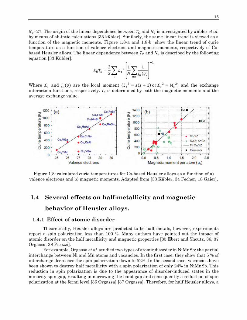
15
𝑁𝑣=27. The origin of the linear dependence between 𝑇𝐶 and 𝑁𝑣 is investigated by 𝑘bler et al.
by means of ab-intio calculations [33 kbler]. Similarly, the same linear trend is viewed as a
function of the magnetic moments. Figure 1.8-a and 1.8-b show the linear trend of curie
temperature as a function of valence electrons and magnetic moments, respectively of Co-
based Heusler alloys. The linear dependence between 𝑇𝐶 and 𝑁𝑣 is described by the following
equation [33 Kübler]:
𝑘𝐵𝑇𝑐 =2
3∑ℒ𝜏
2 [1
𝑁∑
1
𝑗𝑛(𝑞)𝑞𝑛
]
−1
𝜏
Where ℒ𝜏 and 𝑗𝑛(𝑞) are the local moment (ℒ𝜏2 = 𝑠(𝑠 + 1) or ℒ𝜏
2 = 𝑀𝑠2) and the exchange
interaction functions, respectively. 𝑇𝑐 is determined by both the magnetic moments and the
average exchange value.
Figure 1.8: calculated curie temperatures for Co-based Heusler alloys as a function of a)
valence electrons and b) magnetic moments. Adapted from [33 Kbler, 34 Fecher, 18 Gaier].
1.4 Several effects on half-metallicity and magnetic
behavior of Heusler alloys.
1.4.1 Effect of atomic disorder
Theoretically, Heusler alloys are predicted to be half metals, however, experiments
report a spin polarization less than 100 %. Many authors have pointed out the impact of
atomic disorder on the half metallicity and magnetic properties [35 Ebert and Shcutz, 36, 37
Orgassa, 38 Picozzi].
For example, Orgassa et al. studied two types of atomic disorder in NiMnSb: the partial
interchange between Ni and Mn atoms and vacancies. In the first case, they show that 5 % of
interchange decreases the spin polarization down to 52%. In the second case, vacancies have
been shown to destroy half metallicity with a spin polarization of only 24% in NiMnSb. This
reduction in spin polarization is due to the appearance of disorder-induced states in the
minority spin gap, resulting in narrowing the band gap and consequently a reduction of spin
polarization at the fermi level [36 Orgassa] [37 Orgassa]. Therefore, for half Heusler alloys, a

16 Chapter 1: Heusler alloys “state of the art”
suppression of antisite disorder and structural analysis is important to obtain high spin-
polarization [2 Graf].
Galanakis et al. pointed out that the sp elements are not responsible of the minority
gap but important for the structure stability of Heusler alloys. This is illustrated by
substituting Sb in NiMnSb by Sn,In or Te that leads to the destruction of half metallicity [26
Galanakis].
For full Heusler alloys, several groups also studied the effect of atomic disorder on half
metallicity in Co2FeSi [39 Gercsi and Hono], Co2MnGe and Co2MnSi [38 Picozzi]. We will
focus on the atomic disorder and defects effect on the half metallicity in Co2MnSi.
Picozzi et al. investigated different types of defects in Co2MnSi, such as antisites and
atomic swaps in terms of energy formation and defect induced electronic and magnetic
properties. They have found that Mn antisites (Co atoms being replaced by Mn) have the
lowest energy formation and retain the half metallicity character, but the magnetic moment
is reduced by 2 𝜇𝐵. Whereas for Co antisites (Mn atoms being replaced by Co), they have a
slightly higher energy formation and half metallicity is destroyed due to Co antisite d states
and the total magnetic moment is also reduced. For both Mn-Si and Mn-Co swaps, they have
high energy formation and half metallicity is unaffected but the magnetic behavior shows a
reduction down to 4 𝜇𝐵 for Mn-Co swap while the Mn-Si one is not affected and their values
are equal to the ideal L21 phase. [40 Picozzi].
Picozzi et al. have also studied the effect of changing lattice parameters in Co2MnZ
(Z=Si, Ge, Sn) induced by applied pressure. The lattice constant increases as Z atomic number
increases (by 1.8% substituting Ge for Si and by 3.7% substituting Sn for Ge). Thus, the
volume compression leads to an increase of the minority band gap and the fermi energy is
shifted from the valence band into the band gap [38 Picozzi].
1.4.2 Effect of surface and interface
The half metallicity can be lost due to the introduction of surface and interface states
at the fermi level in the minority spin channel. Many theoretical investigations by Ab initio
calculations were performed for half and full Heusler alloys. NiMnSb and Co2MnSi surface
and interface properties were thoroughly studied by several groups [41 Galanakis, 42 Ishida,
43 Nagao, 44 Miura, and 45 Hashemifar]. It is important to note that, experimentally, few
groups have been able to study the surface and interface effects on half metallicity due to
homogeneity, deposition quality conditions, and segregation of atoms to the surface during
the growth of thin films [46 Ristoiu].
Galanakis studied the effect of surface termination on the properties of half (NiMnSb,
CoMnSb and PtMnSb) and full Heusler (Co2MnSi, Co2MnGe and Co2CrAl) alloys [41
Galanakis]. For Co terminated surfaces, a displacement in the spin down state peak near the
fermi level results in a negative state polarization as shown in figure (1.9 c-d). In the case of
Mn(Ge, Si or Cr) terminated surfaces, this strong peak no longer appears as shown in figure
(1.9 a-b). Therefore, it is preferable to have Mn(Ge,Si,Cr) surface termination than Co ones.

17
Figure 1.9: DOS of Co2MnGe and Co2CrAl as function of energy for different terminated
surfaces [41 Galanakis].
Similarly, Ishida et al. have reported that, for Mn-Si surface termination, the half
metallic character is preserved while it is destroyed for Co terminated surface [42 Ishida]. In
their study, they considered two types of planes at the surface of (001) films, the Co and the
MnSi planes. For the Co surface plane, no energy band gap is found for one of the two spin
states, whereas a band gap is found for the MnSi surface plane and hence the half metallicity
is preserved in this surface termination. Hashemifar et al. studied the stability and electronic
structure for different termination surface for Co2MnSi. They have found that the pure Mn
termination preserves the half metallicity of the system [45 Hashemifar].
Besides the surface termination effects on half metallic behavior, the interface role is
of particular importance for spintronic devices where the transport of spin polarized electrons
and holes from one material to another is crucial. As mentioned before, GaAs and MgO are
the two substrates widely used for the deposition of Co2MnSi thin films. For Co2MnSi/GaAs,
Nagao et al. obtained a high spin polarization at (110) CoSi-AsGa interface and a nearly half
metallic behavior is monitored [43 Nagao]. Half metallicity is lost for Mn-Si surface
termination of Co2MnSi/MgO according to Miura et al. [44 Miura]. These effects are related
to the appearance of interface states in the half metallic gap and these states can be filled by
the electrons from the minority valence band [18 Gaier].
Effect of half metallicity on gilbert damping factor
The damping behavior is of particular importance in this thesis and it is important to
shed light on the relation between half metallicity and the gilbert damping factor. More
details about gilbert damping will be discussed in the magnetization dynamics chapter.
In ferromagnetic materials, the Gilbert damping factor 𝛼 is generally accounted to be
proportional to the square of spin orbit coupling, which allows for spin flip transition. The low
damping value 𝛼 is closely related to the half metallicity since the spin gap for minority spins

18 Chapter 1: Heusler alloys “state of the art”
is supposed to avoid spin-flip transition for dynamic magnetic relaxation. The lowest damping
factor obtained theoretically, using extended Hückel tight binding (ETH-TB) model, for
Co2MnSi is 0.6*10-4 [5 liu] and experimentally 9*10-4 [47 Qiao]. Kubota et al. have studied the
half metallic behavior and gilbert damping factor for Co2FexMn1-xSi alloys. In their work, they
monitored the increase in minority DOS at the fermi level and at some point the loss of half
metallic behavior which is accompanied by an increase in gilbert damping factor [48 Kubota].
The gilbert damping factor was found to vary from 0.005 for Co2MnSi (x=0) to 0.02 for Co2FeSi
(x=1) and accompanied by a disappearance of half metallicity for x≥ 0.8.
1.5 Ion irradiation/implantation
In our work, we used ion irradiation to modify the structural properties of Co2MnSi
and study the effect of the structural modifications on the magnetic properties of the alloy as
it will be presented in chapter 5. The purpose of this section is to give an overview of the work
done on different materials by ion irradiation/implantation and its modifications on their
magnetic properties. Additional details about ion irradiation technique will be given in
chapter 3.
Controlling and pattering the magnetic properties of ferromagnetic materials is now a
field of interest for magnonic crystal applications for example. Ion irradiation is a promising
technique that can modify the magnetic behavior through direct modification of the structure
of the investigated material. Irradiation can be done by either heavy or light ions depending
on the mass to charge ratio of the selected ions and the energy of the accelerated ions. For
example, Bonder et al. have reported that irradiation of Ar+ ions at 80 KeV with doses from
1014 to 1016 ions/cm2, is shown to cause intermixing of Co/Pt layers resulting in the
magnetization switching from perpendicular to in plane direction [49 Bonder]. Structural
properties modifications by light ion irradiation, for example, irradiation with He+ ions, of an
energy range of 5-150 KeV due to energy loss of ions trajectory in the solid results in magnetic
patterning as well as interfacial mixing [50 Chappert, 51, 52 Devolder, and 53 Fassebender].
Ion irradiation/implantation have gained interest in studying the modifications of
magnetic materials. Several groups [54 Folks, 55 Fassbender and McCord] have reported the
modification of magnetic parameters upon implantation. For example, Folks et al. have
reported the change in magnetic phase from ferromagnetic state of NiFe alloy films to a
paramagnetic one by Cr ions implantation. As a result, they have patterned continuous
Ni80Fe20 films into separate regions of ferromagnetic and paramagnetic behavior. Fassbender
and McCord have reported a modification of static and dynamic magnetic properties in
Ni81Fe19 by 30 KeV Ni implantation.
Alternatively, He+ irradiation induces an enhancement in the chemical order of FePt and
FePd thin films by increasing the long range L10 order parameter at room temperature [56
Ravelosona, 58 Bernas]. The enhancement of the chemical ordering by He+ ions was done by
Gaier et al. on Heusler alloys and in particular Co2MnSi. In their study they have shown an
improvement of the long range order in the B2 phase [57 Gaier]. This enhancement has been
attributed to the Mn-Co and Co-Si exchanges due to mobile vacancies induced by irradiation
[58 Bernas]. As discussed in this chapter, the disorder influences the structural and magnetic
19
properties and since Heusler alloys exhibit unique magnetic properties, tailoring them is of
particular interest for technological applications.
Another aspect of ion implantation/irradiation is to control the magnetic gilbert damping
coefficient. Several groups have seen an increase in gilbert damping due to ion implantation/
irradiation by Ni and Cr ions respectively [59 Obry, 60 King]. The origin for this increase
relies on local modification of the chemical order in addition to modification of the local
effective field. More details will be given in chapter 5 about the effect of ion irradiation on the
magnetic properties of Heusler alloy Co2MnSi.
1.6 Applications of Heusler alloys
Heusler alloys are known for their high spin polarization, and they have attracted much
interest in the field of spin electronics for their potential application for tunneling
magnetoresistance (TMR) and Giant magnetoresistance (GMR) devices. The half metallic
materials act as a spin filter in such devices which leads to a huge magnetoresistance (MR)
effect [61 Yakushiji]. Tunneling devices with high MR effect can be reached nowadays either
by an engineered insulator barrier or by developing a 100 % spin polarization electrode
materials. The potential candidates for the latter are ferromagnetic oxides or Heusler alloys
[2 Graf]. Several groups have studied Co-based Heusler alloys as electrodes for MTJ, GMR
and for spin injection from ferromagnetic materials into semiconductor. Besides technological
applications, Half Heusler alloys were investigated for energy usages such as Solar cells and
thermoelectric convertors. In the next two paragraphs, a brief description of the mentioned
studies is given.
Tunneling magnetoresistance based on Heusler alloys electrodes was experimentally
reported by Inomata in 2003. In their work, lower Co2Cr0.6Fe0.4Al and upper CoFe electrodes
were used with AlO barrier, thus obtaining a 16 % room temperature rate and 26.5 % at 5 K
[62 Inomata]. Ishikawa et al. have obtained a relatively high TMR ratios of 90% at room
temperature and 192% at 4.2 K using Co-based Heusler alloy MTJs with Co2MnSi as a lower
electrode, MgO as a tunnel barrier prepared by sputtering and Co50Fe50 as an upper electrode
respectively [63 Ishikawa]. Tsunegi et al., in 2009, reported a higher TMR ratio of 217 % at
room temperature and 753 % at 2K for the Co2MnSi/MgO/CoFe TMJs with MgO as a barrier
prepared by sputtering and electron beam evaporation system. The different in reported
values in Co2MnSi/MgO/CoFe TMJs results from the coherent tunneling process through the
crystalline MgO barrier [64 Tsunegi]. Another application for Heusler alloy is the spin
polarized carriers injection into semiconductors. They are considered important in designing
spin injection devices due to several characteristics; such as, high spin polarization at Fermi
energy, high Curie temperature along with large magnetic moments, and their lattice
constants that is close to the III-V semiconductors which makes them ideal for epitaxial
contacts [65 Ambrose, 66 Dong, 67 Lund, and 68 X.Y Dong]. Dong et al. in 2005 have reported
an electrical spin injection of 27% at 2 K for Co2MnGe into Al0.1Ga0.9As/GaAs light emitting
diode hetero structures. However, Co2MnSi with larger minority gap might be an effective
injector than that of Co2MnGe [68 Dong].
Heusler alloys are also useful for energy applications such as solar cells and
thermoelectric convertor. First, for solar cells applications, turning sunlight into electric
energy, Cu-based chalcopyrite semiconductors are used as light absorber materials for low

20 Chapter 1: Heusler alloys “state of the art”
cost thin films. In these conventional chalcopyrite, a CdS buffer layer is sandwiched between
the light absorber and a ZnO window layer. The use of CdS increased the performances of
such devices with record efficiency of 19.9 %. The use of CdS meets the needs for a perfect
contact between the absorber and the other layers with the avoidance of absorption losses,
but CdS is found to be a very toxic material. Therefore, it is needed to replace CdS in solar
systems with new materials of similar crystalline structure to that of chalcopyrite. LiZnP,
LiMgZ (Z=As, P, Pb) and many other half-Heusler alloys fit such category where the electric
conductivity has been shown to increase [69 casper].
Second, thermoelectric convertors (TEC) for power generation aim at reducing CO2 emission
which converts industrial furnaces, gas pipes, waste heat generated by engines and many
more to electricity. The importance of TEC stems from the direct conversion of heat into
electricity leading to a decrease in the reliance on fossil fuels. The existing TEC are inefficient
and expensive at the same time. For that, half-Heusler alloys are interesting for TEC like n-
type NiTiSn, p-type CoTiSb, Sb-doped NiTiSn materials For the latter, power factor can be
reached up to 70 µW (cmK2)-1 at 650 K [70 Bhattacharya].
1.7 Choice of Co2MnSi Heusler compound
Among Heusler alloys, we are interested in studying Co2MnSi compounds because of
their potential compatibility with microelectronic processes, high magnetic moment and
Curie temperature and low damping coefficient. In this section, a brief overview on the
magnetic properties such as saturation magnetization, magneto-crystalline anisotropy,
exchange interaction and damping factor is given.
1.7.1 Saturation Magnetization
Saturation magnetization (Ms) can be defined as the maximum magnetization of a
ferromagnetic material, this results when all the magnetic dipoles are aligned with an
external field or at a remanence state for hard materials. In Table 1.4, we present experiment
vs calculation values of the saturation magnetization of Co2MnSi. The total magnetic moment
experimental values are slightly different from ab-intio calculations.
Ms in Table 1.4 is expressed in 𝜇𝑏 /𝑓. 𝑢 (𝑓𝑜𝑟𝑚𝑢𝑙𝑎 𝑢𝑛𝑖𝑡) ( μB is Bohr’s magneton=9.27× 10⁻²⁴ A.m2), A/m in SI units or Tesla. To convert from μB to A/m or vice versa, we can do the
following:
Ms (A/m) = number of atoms/m3 × 9.27 × 10−24 × (the value of magnetization in μB)
Where the number of atoms/m3 for Co2MnSi = 4 𝑎𝑡𝑜𝑚𝑠 𝑝𝑒𝑟 𝑢𝑛𝑖𝑡 𝑐𝑒𝑙𝑙
𝑎3=
4
5.653= 2.21 × 1028.
𝑚𝑠𝑝𝑖𝑛(μB /𝑓. 𝑢) Co2MnSi
Calculation
5.00 [32
Fujii], [38
Picozzi]
4.96 [13
Brown]
4.94 [25
Galanakis,]
5.008 [26
Galanakis],[71
Galanakis]
𝑚𝑠𝑝𝑖𝑛(μB /𝑓. 𝑢) Co2MnSi
Experiment
5.07 [6
Webster]
5.10±0.04
[72 Raphael]
4.95±0.25
[73 Singh]
4.7 [74
Kämmerer]
5.0 [ 75
Wang]
Table 1.4: calculated and experimental spin magnetic moments per unit cell for Co2MnSi.

21
1.7.2 Magneto-crystalline anisotropy constant
In ferromagnets, the magnetization is generally aligned in a preferential direction,
called the easy axis. The origin of this anisotropy for the direction of the magnetization can
be either from the symmetry of the crystal (magneto crystalline anisotropy) or from dipolar
interaction in the case of shape anisotropy. Our focus will be on the magneto-crystalline
anisotropy of Co2MnSi obtained by several groups.
Magneto-crystalline anisotropy is a consequence of the interaction between orbital
moments and the spins of electrons. In Heusler, the spin-orbit interaction of the localized d-
electrons results in the magneto-crystalline anisotropy. The magnetization will preferentially
align with symmetry axes of the crystal. Anisotropy is described by the anisotropy constant
K which can be experimentally obtained from Ferromagnetic Resonance (FMR), Brillouin
light scattering (BLS) and Magneto-optical Kerr effect (MOKE) and other techniques. In this
thesis, we have employed FMR. In CMS the anisotropy is cubic and the anisotropy constant
K is negative where the easy axis of magnetization lies in the diagonal of the cube. The values
of K range from – 8 KJ/m3 [76 Gaier] to -25 KJ/m3 [77 Ortiz]. . The increase in the anisotropy
constant is related to several effects such as induced strain at the MgO/Co2MnSi interfaces
and to annealing temperatures.
1.7.3 Exchange constant
The origin of the exchange constant will be presented in chapter 2. The purpose of this
paragraph is to give a comparison about the exchange constant obtained for Co2MnSi by
several groups. Ritchie et al. [78 Ritchie] and Rameev et al. [79 Rameev] reported values of
A= 19.3 pJ/m and A= 9.7 pJ/m. Hamrle et al., by BLS measurements, obtained an exchange
value, A= 23.5 pJ/m [80 Hamrle]. By FMR measurements, Pandey et al., Belmeguenai et al.
and Ortiz et al. have reported an exchange value of 21 pJ/m, 27 pJ/m and 19 pJ/m, respectively
[81 Pandey, 82 Belmeguenai, 77 Ortiz]. The differences in reported values are generally
assumed to rely on deposition conditions and substrates effects.
.
1.7.4 Magnetic damping factor
In this thesis, a particular interest is attributed to the study of the magnetic Gilbert
damping factor 𝛼. The latter reflects the time needed for the magnetization pointed out of its
equilibrium position to get back to equilibrium through different kind of relaxation processes.
The dimensionless coefficient 𝛼 is theoretically predicted to be less than 10-3 for Heusler alloys
[5 Liu]. Experimentally, several groups have obtained the Gilbert damping factor, for
example, in the previous work of Ortiz et al., they have found the damping factor value
between 3*10-3 and 7*10-3 [77 Ortiz]. The mentioned values are in agreement with
experimental review about Co-based Heusler alloys by Trudel et al. [8 Trudel]. Chapter two
will give some basics of relaxation mechanisms and chapter 4 and 5 will present the results
obtained on the dynamic magnetic properties and specially the Gilbert damping factor.

22 Chapter 1: Heusler alloys “state of the art”
Figure 1.10: schematic presentation of Co2MnSi crystalline structure: a) L21, b) B2, c) D03
and A2 phases.
In conclusion of this section, the magnetic behavior of these alloys depend strongly on
their structural properties (figure 1.10). The magnetic behavior of L21 and B2 phases are
similar, at least for the magnetic moment and spin polarization but no information is given
on their respective anisotropy nor on the damping in the B2 order. Theoretically Picozzi et al
[6 Picozzi] have shown that in the L21 phase, the value of magnetization is 5 𝜇𝑏 /𝑓. 𝑢. (1.3 T)
and also when Mn and Si swap their positions in the lattice to form the B2 phase. The half
metallicity of CMS is shown theoretically with a band gap at the fermi level for the L21 phase
(0.81 eV) [38 Picozzi]. Furthermore [ 5 Liu] has calculated with the Fermi Breathing
method a low Gilbert damping coefficient of 6*10-5 for this phase. Whereas a cubic
crystal anisotropy is present in CMS, the anisotropy constant is negative leading to a
magnetic easy axis oriented in the diagonal of the cube (<111>) and the hard axis along the
edge of the cube (<100>). While there are many information about the L21 and B2 phases,
insufficient literature is conducted on both D03 and A2 phases. Theoretically, Picozzi also
studied the effect D03 order on the average magnetization when Co and Mn swap their
positions. He also shows a decrease in the saturation magnetization to 4.5 𝜇𝑏 /𝑓. 𝑢. (1.16 T)
whereas no information about the cubic anisotropy nor the damping relaxation terms is given.
For the A2 phase no information was found about the magnetic behavior of this completely
disordered phase.

23
Chapter 1 References:
[1] “F. Heusler, W. Starck, and E. Haupt, Verh. DPG 5, 220 (1903).”
[2] T. Graf, C. Felser, and S. S. P. Parkin, “Simple rules for the understanding of Heusler
compounds,” Prog. Solid State Chem., vol. 39, no. 1, pp. 1–50, May 2011.
[3] R. A. De Groot, F. M. Mueller, P. G. Van Engen, and K. H. J. Buschow, “New class of
materials: half-metallic ferromagnets,” Phys. Rev. Lett., vol. 50, no. 25, pp. 2024–2027,
1983.
[4] K. Bartholomé, B. Balke, D. Zuckermann, M. Köhne, M. Müller, K. Tarantik, and J.
König, “Thermoelectric Modules Based on Half-Heusler Materials Produced in Large
Quantities,” J. Electron. Matter., vol. 43, no. 6, pp. 1775–1781, Nov. 2013.
[5] C. Liu, C. K. A. Mewes, M. Chshiev, T. Mewes, and W. H. Butler, “Origin of low Gilbert
damping in half metals,” Appl. Phys. Lett., vol. 95, no. 2, p. 022509, 2009.
[6] P. J. Webster, “Magnetic and chemical order in Heusler alloys containing cobalt and
manganese,” J. Phys. Chem. Solids, vol. 32, no. 6, pp. 1221–1231, 1971.
[7] G. E. Bacon and J. S. Plant, “Chemical ordering in Heusler alloys with the general formula
A2BC or ABC,” J. Phys. F Met. Phys., vol. 1, no. 4, p. 524, Jul. 1971.
[8] S. Trudel, O. Gaier, J. Hamrle, and B. Hillebrands, “Magnetic anisotropy, exchange and
damping in cobalt-based full-Heusler compounds: an experimental review,” J. Phys. Appl.
Phys., vol. 43, no. 19, p. 193001, 2010.
[9] K. Kobayashi, K. Ishikawa, R. Y. Umetsu, R. Kainuma, K. Aoki, and K. Ishida, “Phase
stability of B2 and L21 ordered phases in Co2YGa (Y=Ti, V, Cr, Mn, Fe) alloys,” J. Magn.
Magn. Mater., vol. 310, no. 2, Part 2, pp. 1794–1795, Mar. 2007.
[10] H. C. Kandpal, G. H. Fecher, and C. Felser, “Calculated electronic and magnetic
properties of the half-metallic, transition metal based Heusler compounds,” J. Phys. Appl.
Phys., vol. 40, no. 6, p. 1507, Mar. 2007.
[11] H. J. Elmers, S. Wurmehl, G. H. Fecher, G. Jakob, C. Felser, and G. Schonhense, “Field
dependence of orbital magnetic moments in the Heusler compounds Co 2 FeAl and Co 2
Cr 0.6 Fe 0.4 Al,” Appl. Phys. Mater. Sci. Process., vol. 79, no. 3, pp. 557–563, Aug. 2004.
[12] S. Wurmehl, G. H. Fecher, H. C. Kandpal, V. Ksenofontov, C. Felser, H.-J. Lin, and J.
Morais, “Geometric, electronic, and magnetic structure of Co 2 FeSi : Curie temperature
and magnetic moment measurements and calculations,” Phys. Rev. B, vol. 72, no. 18, Nov.
2005.
[13] P. J. Brown, K. U. Neumann, P. J. Webster, and K. R. A. Ziebeck, “The magnetization
distributions in some Heusler alloys proposed as half-metallic ferromagnets,” J. Phys.
Condens. Matter, vol. 12, no. 8, p. 1827, 2000.
[14] K. H. J. Buschow, P. G. van Engen, and R. Jongebreur, “Magneto-optical properties of
metallic ferromagnetic materials,” J. Magn. Magn. Matter., vol. 38, no. 1, pp. 1–22, août
1983.
[15] G. Li, T. Taira, K. Matsuda, M. Arita, T. Uemura, and M. Yamamoto, “Epitaxial
growth of Heusler alloy Co2MnSi/MgO heterostructures on Ge(001) substrates,” Appl.
Phys. Lett., vol. 98, no. 26, p. 262505, Jun. 2011.
[16] M. a. I. Nahid, M. Oogane, H. Naganuma, and Y. Ando, “Epitaxial growth of Co2MnSi
thin films at the vicinal surface of n-Ge(111) substrate,” Appl. Phys. Lett., vol. 96, no. 14,
p. 142501, Apr. 2010.

24 Chapter 1: Heusler alloys “state of the art”
[17] G. Ortiz, A. Garcia-Garcia, N. Biziere, F. Boust, J. F. Bobo, et E. Snoeck, « Growth,
structural, and magnetic characterization of epitaxial Co2MnSi films deposited on MgO
and Cr seed layers », J. Appl. Phys., vol. 113, no 4, p. 043921, 2013..
[18] O. Gaier, “A study of exchange interaction, magnetic anisotropies, and ion beam
induced effects in thin films of Co2-based Heusler compounds,” Ph. D. dissertation,
Technical University of Kaiserslautern, 2009.
[19] C. Magen, E. Snoeck, U. Lüders, and J. F. Bobo, “Effect of metallic buffer layers on the
antiphase boundary density of epitaxial Fe3O4,” J. Appl. Phys., vol. 104, no. 1, p. 013913,
Jul. 2008.
[20] A. García-Garcia, J. A. Pardo, P. Štrichovanec, C. Magén, A. Vovk, J. M. D. Teresa, G.
N. Kakazei, Y. G. Pogorelov, L. Morellón, P. A. Algarabel, and M. R. Ibarra, “Tunneling
magnetoresistance in epitaxial discontinuous Fe/MgO multilayers,” Appl. Phys. Lett., vol.
98, no. 12, p. 122502, Mar. 2011.
[21] “Soulen R J Jr et al 1998 Science 282 85.”
[22] H. Kato, T. Okuda, Y. Okimoto, Y. Tomioka, K. Oikawa, T. Kamiyama, and Y. Tokura,
“Structural and electronic properties of the ordered double perovskites A 2 M ReO 6 ( A
=Sr,Ca; M =Mg,Sc,Cr,Mn,Fe,Co,Ni,Zn),” Phys. Rev. B, vol. 69, no. 18, May 2004.
[23] T. Shishidou, A. J. Freeman, and R. Asahi, “Effect of GGA on the half-metallicity of
the itinerant ferromagnet CoS 2,” Phys. Rev. B, vol. 64, no. 18, Oct. 2001.
[24] “http://www.nims.go.jp/apfim/halfmetal.html.”
[25] I. Galanakis, P. H. Dederichs, and N. Papanikolaou, “Slater-Pauling behavior and origin
of the half-metallicity of the full-Heusler alloys,” Phys. Rev. B, vol. 66, no. 17, p. 174429,
Nov. 2002.
[26] I. Galanakis, P. Mavropoulos, and P. H. Dederichs, “Electronic structure and Slater–
Pauling behaviour in half-metallic Heusler alloys calculated from first principles,” J.
Phys. Appl. Phys., vol. 39, no. 5, pp. 765–775, Mar. 2006.
[27] W. E. Pickett, “Single spin superconductivity,” Phys. Rev. Lett., vol. 77, no. 15, p. 3185,
1996.
[28] F. Casper, T. Graf, S. Chadov, B. Balke, and C. Felser, “Half-Heusler compounds: novel
materials for energy and spintronic applications,” Semicond. Sci. Technol., vol. 27, no. 6,
p. 063001, Jun. 2012.
[29] J. C. Slater, “The Ferromagnetism of Nickel. II. Temperature Effects,” Phys. Rev., vol.
49, no. 12, pp. 931–937, juin 1936.
[30] L. Pauling, “The nature of the interatomic forces in metals,” Phys. Rev., vol. 54, no. 11,
p. 899, 1938.
[31] Y. Kurtulus, R. Dronskowski, G. Samolyuk, and V. Antropov, “Electronic structure
and magnetic exchange coupling in ferromagnetic full Heusler alloys,” Phys. Rev. B, vol.
71, no. 1, Jan. 2005.
[32] S. Fujii, S. Sugimura, and S. Asano, “Hyperfine fields and electronic structures of the
Heusler alloys Co2MnX (X= Al, Ga, Si, Ge, Sn),” J. Phys. Condens. Matter, vol. 2, no. 43,
p. 8583, 1990.
[33] J. Kübler, A. R. William, and C. B. Sommers, “Formation and coupling of magnetic
moments in Heusler alloys,” Phys. Rev. B, vol. 28, no. 4, pp. 1745–1755, août 1983.
J. Kübler, “Ab initio estimates of the Curie temperature for magnetic compounds,” J.
Phys. Condens. Matter, vol. 18, no. 43, p. 9795, 2006.
[34] G. H. Fecher, H. C. Kandpal, S. Wurmehl, C. Felser, and G. Schönhense, “Slater-
Pauling rule and Curie temperature of Co2-based Heusler compounds,” J. Appl. Phys.,
vol. 99, no. 8, p. 08J106, Apr. 2006.
25
[35] H. Ebert and G. Schütz, “Theoretical and experimental study of the electronic
structure of PtMnSb,” J. Appl. Phys., vol. 69, no. 8, pp. 4627–4629, Apr. 1991.
[36] D. Orgassa, H. Fujiwara, T. C. Schulthess, and W. H. Butler, “First-principles
calculation of the effect of atomic disorder on the electronic structure of the half-metallic
ferromagnet NiMnSb,” Phys. Rev. B, vol. 60, no. 19, pp. 13237–13240, Nov. 1999.
[37] D. Orgassa, H. Fujiwara, T. C. Schulthess, and W. H. Butler, “Disorder dependence of
the magnetic moment of the half-metallic ferromagnet NiMnSb from first principles,” J.
Appl. Phys., vol. 87, no. 9, pp. 5870–5871, May 2000.
[38] S. Picozzi, A. Continenza, and A. J. Freeman, “Co2MnX (X=Si, Ge, Sn) Heusler
compounds: An ab-initio study of their structural, electronic, and magnetic properties at
zero and elevated pressure,” Phys. Rev. B, vol. 66, no. 9, p. 094421, Sep. 2002.
[39] Z. Gercsi and K. Hono, “Ab initio predictions for the effect of disorder and quarternary
alloying on the half-metallic properties of selected Co2Fe-based Heusler alloys,” J. Phys.
Condens. Matter, vol. 19, no. 32, p. 326216, Jul. 2007.
[40] S. Picozzi, A. Continenza, and A. Freeman, “Role of structural defects on the half-
metallic character of Co2MnGe and Co2MnSi Heusler alloys,” Phys. Rev. B, vol. 69, no. 9,
Mar. 2004.
[41] I. Galanakis, “Surface properties of the half-and full-Heusler alloys,” J. Phys. Condens.
Matter, vol. 14, no. 25, p. 6329, Jul. 2002.
[42] S. Ishida, T. Masaki, S. Fujii, and S. Asano, “Theoretical search for half-metalliic films
of Co2MnZ (Z = Si, Ge),” Phys. B Condens. Matter, vol. 245, no. 1, pp. 1–8, Jan. 1998.
[43] K. Nagao, Y. Miura, and M. Shirai, “Half-metallicity at the (110) interface between a
full Heusler alloy and GaAs,” Phys. Rev. B, vol. 73, no. 10, p. 104447, Mar. 2006.
[44] Y. Miura, H. Uchida, Y. Oba, K. Nagao, and M. Shirai, “Coherent tunnelling
conductance in magnetic tunnel junctions of half-metallic full Heusler alloys with MgO
barriers,” J. Phys. Condens. Matter, vol. 19, no. 36, p. 365228, Sep. 2007.
[45] S. J. Hashemifar, P. Kratzer, and M. Scheffler, “Preserving the Half-Metallicity at the
Heusler Alloy C o 2 M n S i ( 001 ) Surface: A Density Functional Theory Study,” Phys.
Rev. Lett., vol. 94, no. 9, Mar. 2005.
[46] D. Ristoiu, J. P. Nozières, C. N. Borca, T. Komesu, H. –. Jeong, and P. A. Dowben, “The
surface composition and spin polarization of NiMnSb epitaxial thin films,” EPL Europhys.
Lett, vol. 49, no. 5, p. 624, Mar. 2000.
[47] S.-Z. Qiao, J. Zhang, Y.-F. Qin, R.-R. Hao, H. Zhong, D.-P. Zhu, Y. Kang, S.-S. Kang,
S.-Y. Yu, G.-B. Han, S.-S. Yan, and L.-M. Mei, “Structural and Magnetic Properties of Co
2 MnSi Thin Film with a Low Damping Constant,” Chin. Phys. Lett., vol. 32, no. 5, p.
057601, May 2015.
[48] T. Kubota, S. Tsunegi, M. Oogane, S. Mizukami, T. Miyazaki, H. Naganuma, and Y.
Ando, “Half-metallicity and Gilbert damping constant in Co2FexMn1−xSi Heusler alloys
depending on the film composition,” Appl. Phys. Lett., vol. 94, no. 12, p. 122504, Mar.
2009.
[49] M. J. Bonder, N. D. Telling, P. J. Grundy, C. A. Faunce, T. Shen, and V. M. Vishnyakov,
“Ion irradiation of Co/Pt multilayer films,” J. Appl. Phys., vol. 93, no. 10, pp. 7226–7228,
May 2003.
[50] C. Chappert, “Planar Patterned Magnetic Media Obtained by Ion Irradiation,”
Science, vol. 280, no. 5371, pp. 1919–1922, Jun. 1998.
[51] T. Devolder, “Light ion irradiation of Co/Pt systems: structural origin of the
decrease in magnetic anisotropy,” Physical Review B, vol. 62, no. 9, p. 5794, 2000.

26 Chapter 1: Heusler alloys “state of the art”
[52] T. Devolder, J. Ferré, C. Chappert, H. Bernas, J.-P. Jamet, and V. Mathet,
“Magnetic properties of He + -irradiated Pt/Co/Pt ultrathin films,” Physical Review
B, vol. 64, no. 6, Jul. 2001
[53] J. Fassbender, D. Ravelosona, and Y. Samson, “Tailoring magnetism by light-ion
irradiation,” J. Phys. Appl. Phys., vol. 37, no. 16, p. R179, Aug. 2004.
[54] L. Folks, R. E. Fontana, B. A. Gurney, J. R. Childress, S. Maat, J. A. Katine, J. E. E.
Baglin, and A. J. Kellock, “Localized magnetic modification of permalloy using Cr+ ion
implantation,” J. Phys. Appl. Phys., vol. 36, no. 21, p. 2601, 2003.
[55] J. Fassbender and J. McCord, “Control of saturation magnetization, anisotropy, and
damping due to Ni implantation in thin Ni[sub 81]Fe[sub 19] layers,” Appl. Phys. Lett.,
vol. 88, no. 25, p. 252501, 2006.
[56] D. Ravelosona, C. Chappert, V. Mathet, and H. Bernas, “Chemical order induced by
ion irradiation in FePt (001) films,” Appl. Phys. Lett., vol. 76, no. 2, p. 236, 2000.
[57] O. Gaier, J. Hamrle, B. Hillebrands, M. Kallmayer, P. Pörsch, G. Schönhense, H. J.
Elmers, J. Fassbender, A. Gloskovskii, C. A. Jenkins, C. Felser, E. Ikenaga, Y. Sakuraba,
S. Tsunegi, M. Oogane, and Y. Ando, “Improvement of structural, electronic, and magnetic
properties of Co2MnSi thin films by He+ irradiation,” Appl. Phys. Lett., vol. 94, no. 15, p.
152508, Apr. 2009.
[58] H. Bernas, J.-P. Attané, K.-H. Heinig, D. Halley, D. Ravelosona, A. Marty, P. Auric, C.
Chappert, and Y. Samson, “Ordering Intermetallic Alloys by Ion Irradiation: A Way to
Tailor Magnetic Media,” Phys. Rev. Lett., vol. 91, no. 7, Aug. 2003.
[59] B. Obry, T. Meyer, P. Pirro, T. Brächer, B. Lägel, J. Osten, T. Strache, J. Fassbender,
and B. Hillebrands, “Microscopic magnetic structuring of a spin-wave waveguide by ion
implantation in a Ni81Fe19 layer,” Appl. Phys. Lett., vol. 102, no. 2, p. 022409, 2013.
[60] J. A. King, A. Ganguly, D. M. Burn, S. Pal, E. A. Sallabank, T. P. A. Hase, A. T.
Hindmarch, A. Barman, and D. Atkinson, “Local control of magnetic damping in
ferromagnetic/non-magnetic bilayers by interfacial intermixing induced by focused ion-
beam irradiation,” Appl. Phys. Lett., vol. 104, no. 24, p. 242410, Jun. 2014.
[61] K. Yakushiji, K. Saito, S. Mitani, K. Takanashi, Y. K. Takahashi, and K. Hono,
“Current-perpendicular-to-plane magnetoresistance in epitaxial Co2MnSi∕Cr∕Co2MnSi
trilayers,” Appl. Phys. Lett., vol. 88, no. 22, p. 222504, May 2006..
[62] K. Inomata, N. Ikeda, N. Tezuka, R. Goto, S. Sugimoto, M. Wojcik, and E. Jedryka,
“Highly spin-polarized materials and devices for spintronics,” Sci. Technol. Adv. Mater.,
vol. 9, no. 1, p. 014101, Jan. 2008.
[63] T. Ishikawa, T. Marukame, H. Kijima, K.-I. Matsuda, T. Uemura, M. Arita, and M.
Yamamoto, “Spin-dependent tunneling characteristics of fully epitaxial magnetic
tunneling junctions with a full-Heusler alloy Co2MnSi thin film and a MgO tunnel
barrier,” Appl. Phys. Lett., vol. 89, no. 19, p. 192505, Nov. 2006.
[64] S. Tsunegi, Y. Sakuraba, M. Oogane, N. D. Telling, L. R. Shelford, E. Arenholz, G. van
der Laan, R. J. Hicken, K. Takanashi, and Y. Ando, “Tunnel magnetoresistance in
epitaxially grown magnetic tunnel junctions using Heusler alloy electrode and MgO
barrier,” J. Phys. Appl. Phys., vol. 42, no. 19, p. 195004, Oct. 2009.
[65] T. Ambrose, J. J. Krebs, and G. A. Prinz, “Epitaxial growth and magnetic properties
of single-crystal Co2MnGe Heusler alloy films on GaAs (001),” Appl. Phys. Lett., vol. 76,
no. 22, pp. 3280–3282, May 2000.

27
[66] J. W. Dong, L. C. Chen, C. J. Palmstro/m, R. D. James, and S. McKernan, “Molecular
beam epitaxy growth of ferromagnetic single crystal (001) Ni2MnGa on (001) GaAs,” Appl.
Phys. Lett., vol. 75, no. 10, pp. 1443–1445, Sep. 1999.
[68] M. S. Lund, J. W. Dong, J. Lu, X. Y. Dong, C. J. Palmstrøm, and C. Leighton,
“Anomalous magnetotransport properties of epitaxial full Heusler alloys,” Appl. Phys.
Lett., vol. 80, no. 25, pp. 4798–4800, Jun. 2002.
[68] X. Y. Dong, C. Adelmann, J. Q. Xie, C. J. Palmstrøm, X. Lou, J. Strand, P. A. Crowell, J.-
P. Barnes, and A. K. Petford-Long, “Spin injection from the Heusler alloy Co2MnGe into
Al0.1Ga0.9As∕GaAs heterostructures,” Appl. Phys. Lett., vol. 86, no. 10, p. 102107, Mar.
2005.
[69] F. Casper, T. Graf, S. Chadov, B. Balke, and C. Felser, “Half-Heusler compounds: novel
materials for energy and spintronic applications,” Semicond. Sci. Technol., vol. 27, no. 6,
p. 063001, Jun. 2012.
[70] S. Bhattacharya, A. L. Pope, R. T. L. Iv, T. M. Tritt, V. Ponnambalam, Y. Xia, and S.
J. Poon, “Effect of Sb doping on the thermoelectric properties of Ti-based half-Heusler
compounds, TiNiSn1−xSbx,” Appl. Phys. Lett., vol. 77, no. 16, pp. 2476–2478, Oct. 2000
[71] I. Galanakis, “Orbital magnetism in the half-metallic Heusler alloys,” Phys. Rev. B,
vol. 71, no. 1, Jan. 2005
[72] M. P. Raphael, B. Ravel, Q. Huang, M. A. Willard, S. F. Cheng, B. N. Das, R. M. Stroud,
K. M. Bussmann, J. H. Claassen, and V. G. Harris, “Presence of antisite disorder and its
characterization in the predicted half-metal Co 2 MnSi,” Phys. Rev. B, vol. 66, no. 10, Sep.
2002.
[73] L. J. Singh, Z. H. Barber, Y. Miyoshi, W. R. Branford, and L. F. Cohen, “Structural
and transport studies of stoichiometric and off-stoichiometric thin films of the full Heusler
alloy Co2MnSi,” J. Appl. Phys., vol. 95, no. 11, pp. 7231–7233, Jun. 2004
[74] S. Kämmerer, A. Thomas, A. Hütten, and G. Reiss, “Co2MnSi Heusler alloy as
magnetic electrodes in magnetic tunnel junctions,” Appl. Phys. Lett., vol. 85, no. 1, pp. 79–
81, Jul. 2004
[75] W. H. Wang, M. Przybylski, W. Kuch, L. I. Chelaru, J. Wang, Y. F. Lu, J. Barthel, H.
L. Meyerheim, and J. Kirschner, “Magnetic properties and spin polarization of
$\mathrmCo_2\mathrmMnSi$ Heusler alloy thin films epitaxially grown on
GaAs(001),” Phys. Rev. B, vol. 71, no. 14, p. 144416, avril 2005.
[76] O. Gaier, J. Hamrle, S. J. Hermsdoerfer, H. Schultheiß, B. Hillebrands, Y. Sakuraba,
M. Oogane, and Y. Ando, “Influence of the L21 ordering degree on the magnetic properties
of Co2MnSi Heusler films,” J. Appl. Phys., vol. 103, no. 10, p. 103910, May 2008
[77] G. Ortiz, A. Garcia, J. Ben Youssef, N. Biziere, F. Boust, J. Bobo, E. Snoeck, and N.
Vukadinovic, “Broadband Ferromagnetic Resonance Study of Thin Films: Effect of the
Film Thickness,” IEEE Trans. Magn., vol. 49, no. 3, pp. 1037–1040, Mar. 2013
[78] L. Ritchie, G. Xiao, Y. Ji, T. Y. Chen, C. L. Chien, M. Zhang, J. Chen, Z. Liu, G. Wu,
and X. X. Zhang, “Magnetic, structural, and transport properties of the Heusler alloys Co
2 MnSi and NiMnSb,” Phys. Rev. B, vol. 68, no. 10, Sep. 2003.
[79] B. Rameev, F. Yildiz, S. Kazan, B. Aktas, A. Gupta, L. R. Tagirov, D. Rata, D. Buergler,
P. Gruenberg, C. M. Schneider, S. Kämmerer, G. Reiss, et A. Hütten, « FMR

28 Chapter 1: Heusler alloys “state of the art”
investigations of half-metallic ferromagnets », Phys. Status Solidi A, vol. 203, no 7, p.
1503‑1512, mai 2006.
[80] J. Hamrle, O. Gaier, S.-G. Min, B. Hillebrands, Y. Sakuraba, and Y. Ando,
“Determination of exchange constants of Heusler compounds by Brillouin light scattering
spectroscopy: application to Co2MnSi,” J. Phys. Appl. Phys., vol. 42, no. 8, p. 084005, Apr.
2009.
[81] H. Pandey, P. C. Joshi, R. P. Pant, R. Prasad, S. Auluck, and R. C. Budhani, “Evolution
of ferromagnetic and spin-wave resonances with crystalline order in thin films of full-
Heusler alloy Co2MnSi,” J. Appl. Phys., vol. 111, no. 2, p. 023912, Jan. 2012.
[82] M. Belmeguenai, F. Zighem, D. Faurie, H. Tuzcuoglu, S.-M. Chérif, P. Moch, K.
Westerholt, and W. Seiler, “Structural and magnetic properties of Co2MnSi thin films,”
Phys. Status Solidi A, vol. 209, no. 7, pp. 1328–1333, juillet 2012.

29
Chapter 2: Magnetization
Dynamics
In this chapter, we start with the Basics of magnetism presented in section 2.1, then
the different magnetic energies in a ferromagnetic system are introduced in section 2.2.
Section 2.3 presents the theoretical aspects of magnetization dynamics along with the
solution equation of motion with and without relaxation mechanisms. Ferromagnetic
resonance, magnetostatic modes and spin waves will be discussed in section 2.4. Finally we
will focus on the extrinsic and intrinsic relaxation processes of magnetization relaxation in
section 2.5. The reader is addressed to these several books for additional information
regarding the mentioned topics [1 Coey, 2 Blundel, 3 Stancil and Prabhakar, 4 Gurevich and
Melkov, 5 Vonsovskii, and 6 Getzlaff].
2.1 Basics of Magnetism
A magnetic dipole moment is formed when an electron orbits around the nucleus, creating
a current loop of an area A, and expressed as 𝝁 = 𝑰 𝑨 . The magnetic moment can be also
expressed by the orbital angular momentum of electrons, L, then the magnetic dipole moment
can be written as 𝝁 = −𝒆
𝟐𝒎𝑳 . For an electron, the angular momentum 𝑳 is due to orbital
motion of the electron 𝒍 and to an intrinsic property called spin′ ′ (Figure 2.1).
Figure 2.1: The magnetic moment of an atom is contributed by both the orbital and spin
magnetic motion of the electron.
Both the orbital and spin angular momentum contribute to the magnetic moment of an
electron. We can define 𝝁𝒍 and 𝝁𝒔 as the orbital magnetic moment and spin magnetic

30 Chapter 2: Magnetization dynamics
moment, respectively. To derive both 𝝁𝒍 and 𝝁𝑺 expressions, the angular momentum 𝑳 is
described by quantum mechanical theory, 𝑳 = 𝒎𝒍 ħ where 𝒎𝒍 is an orbital quantum number
that varies from - 𝒍 to 𝒍. Substituting 𝒎𝒍 ħ in the expression of magnetic dipole moment we
get:
𝝁𝒍 = − 𝝁𝑩 𝒎𝒍 is the orbital magnetic moment and 𝝁𝑩 =𝒆 ħ
𝟐𝒎= 9.27 × 10⁻²⁴ 𝐴. 𝑚2, is the Bohr
magneton.
𝝁𝑺 = − 𝒈 𝝁𝑩 𝒎𝒔 is the spin magnetic moment, 𝒎𝒔 is the electron spin quantum number and
𝒈 ≈ 𝟐. 𝟎𝟎𝟑 is the Landé factor or also called the spectroscopic splitting factor.
Therefore, from the above two expressions we can define the total magnetic moment, due to
both orbital and spin contribution, as:
𝝁𝑻𝒐𝒕𝒂𝒍 = − 𝝁𝑩( ∑ 𝒎𝒊 𝒍 + 𝒈∑ 𝒎𝒊 𝒔
). (2.1)
The magnetization M (A.m) is defined as the sum of all magnetic moments per unit volume
V.
𝑴 =∑ 𝝁𝑻𝒐𝒕𝒂𝒍
𝑽 (2.2)
Let us consider a material placed in a magnetic field, the response of the atomic
moments to that external field will define the material’s magnetic behavior. The magnetic
behavior of any matter in an external field is dived into the following categories (Figure 2.2):
Figure 2.2: a) the atomic dipole moment for a a) diamagnetic and b) paramagnetic material
with and without an external magnetic field. The alignment of magnetic moments in c)
ferromagnetic and d) antiferromagnetic materials.
Diamagnetic materials: In the absence of the external magnetic field, no dipoles exist; but
in the presence of an external magnetic field, magnetic dipoles are induced to counterbalance
the applied magnetic flux. They align in opposite direction to the applied field resulting in a

31
negative non-zero magnetic moment. The magnetic susceptibility is then negative for such
materials and of the order of 10-6 to 10-5.
Paramagnetic materials: in the absence of external magnetic field, the paramagnetic
materials possess magnetic moments that are randomly distributed due to thermal
agitations. When applying an external magnetic field, these atomic dipoles align with the
applied field and a positive net magnetization appears. The susceptibility is positive with
values between 10-5 and 10-4.
Ferromagnetic materials: In these materials, the exchange interaction (see below) is
responsible for the parallel alignment of the magnetic moments on a length scale called the
exchange length. The order of magnitude of exchange length is few nanometers (for example:
1.5 nm for Fe and 3.37 nm for Co). At the macroscopic scale, ferromagnetic materials can
either present a net magnetization or not. In the latter case, the magnetization is organized
in domains with different orientations in order to minimize the magnetic stray field. So even
with a zero net magnetization, there is a local magnetization in each domain.
The susceptibility of ferromagnetic materials is generally from 10 to several thousands. These
materials are classified as soft or hard depending on their ability to switch the magnetization
from one direction to another opposite one.
Magnetic materials can be characterized by a hysteresis loop as shown in Figure 2.3.
Moreover, the thermal behavior of ferromagnetic materials is important; above a given
temperature, called the Curie temperature, the exchange interaction is not sufficient to
maintain the alignment of the magnetic moments and therefore the material becomes
paramagnetic.
Figure 2.3: a) A sufficient magnetic field is applied to reach saturation magnetization inside
a ferromagnetic material, then in b), the magnetic field is being reduced until there is no
external field where a part of the material still have a residual magnetization. In c), to

32 Chapter 2: Magnetization dynamics
completely demagnetize the material a significant field is needed and is called coercive field.
In d) the sample is saturated in the opposite direction.
Ferri and Antiferro magnetic materials: these materials are generally composed of two
ferromagnetic sub-lattices that are coupled antiparallel. If each sub-lattice presents the same
magnetic moment (+M and –M) then the net magnetization is null and we have an
antiferromagnetic material. Unlike ferromagnets, above a temperature called Neel
temperature, they become paramagnetic. If the two sub-lattices moments are uncompensated
we have then a nonzero net magnetization. These materials are called ferrimagnetic.
2.2 Micro-magnetic energy terms of ferromagnetic thin
films
In a ferromagnetic material, the equilibrium position of the magnetization is found when
the magnetization is aligned with the effective field defined as:
𝑯𝒆𝒇𝒇 = −𝟏
𝝁𝟎
𝜹𝑬𝒕𝒐𝒕
𝜹𝑴 (2.3)
𝑬𝒕𝒐𝒕 is the total free energy of a ferromagnetic material, 𝝁𝟎 is the vacuum permeability (𝝁𝟎 =4𝜋 ∗ 10−7) and 𝑴 is the total magnetization. Different energy terms contribute the total
energy of a ferromagnetic material. A stable state is reached when the energy is minimized.
The main energy terms we will focus on are the Zeeman, exchange, demagnetization, and
magneto-crystalline energies.
𝑬𝒕𝒐𝒕 = 𝑬𝒁𝒆𝒆𝒎𝒂𝒏 + 𝑬𝒆𝒙𝒄𝒉𝒂𝒏𝒈𝒆 + 𝑬𝒅𝒆𝒎𝒂𝒈 + 𝑬𝒂𝒏𝒊𝒔𝒐𝒕𝒓𝒐𝒑𝒚 (2.4)
2.2.1 Zeeman Energy The magnetic moments within the sample will align parallel to an applied field to
minimize the energy of the system. This behavior is known as the Zeeman energy expressed
in the following equation:
𝑬𝒛𝒆𝒆𝒎𝒂𝒏 = −𝝁𝟎 ∫ 𝒆𝒙𝒕. 𝒅𝑽 (2.5)
2.2.2 Exchange energy The exchange interaction is mediated by different mechanisms depending on the
material system. In ferromagnetic material, the parallel alignment of the spins is the direct
exchange interaction. This one comes from the competition of the coulomb interaction of the
two electrons and the Pauli Exclusion Principle.
Considering two spins (𝒔𝒊 𝑎𝑛𝑑 𝒔𝒋 ), the Hamiltonian of the system including the exchange
interaction can be expressed as:
𝑯𝒊𝒋 = −𝟐 𝑱 𝑺𝒊𝑺𝒋 (2.6)

33
𝑯𝒊𝒋 is the exchange Hamiltonian for two interacting spins 𝑺𝒊 𝑎𝑛𝑑 𝑺𝒋, 𝑱 is the exchange integral
that depends on the material and the interatomic distances (i.e. Orbital overlap). If 𝑱 is
positive, then the energy is minimum for parallel alignment of the spins, leading to the
ferromagnetic order. If 𝑱 is negative, then the minimum energy results in an antiparallel
alignment of the spins and hence an antiferromagnetic behavior. This is illustrated by the
Bethe-Slater curve in Figure 2.4 [6 Getzlaff].
Figure 2.4: The Bethe-Slater curve. Exchange integral vs. the ratio of interatomic distance
𝒓𝒂𝒃 to the radius of d shell 𝒓𝒅 [fundamentals of magnetism]. Mn and Cr are examples of an
antiferromagnetic materials with negative exchange integral while Fe,Co and Ni are
ferromagnetic with a positive exchange integral.
In the general case of two spins presenting a relative angle, the cost in exchange energy can
be expressed as:
𝑬𝒆𝒙𝒄𝒉𝒂𝒏𝒈𝒆 = −𝟐 𝑱 𝑺𝟐∑ 𝑪𝒐𝒔𝜽𝒊𝒋𝒊𝒋 (2.7)
Where 𝜽𝒊𝒋 is the angle between the spins i and j. In the continuum approach defining the
micro magnetism, the exchange energy, in a certain volume of a crystal, is written as:
𝑬𝒆𝒙𝒄𝒉𝒂𝒏𝒈𝒆 = 𝑨∫(𝛁𝒎𝒙 + 𝛁𝒎𝒚 + 𝛁𝒎𝒛)𝟐 𝒅𝑽 (2.8)
𝒎𝒙, 𝒎𝒚 and 𝒎𝒛 are the direction cosines of magnetization with respect to the crystal axis. 𝑨
is the exchange stiffness constant of the material. 𝑨 = (𝒄 𝑱 𝑺𝟐)/𝒂, 𝒄 is a crystallographic
structure dependent constant and 𝒂 is the lattice parameter. 𝑨 is expressed in Joules/meters.
The above equation can be written as a function of the exchange field 𝑒𝑥𝑐ℎ𝑎𝑛𝑔𝑒 defined as
follows:
𝑬𝒆𝒙𝒄𝒉𝒂𝒏𝒈𝒆 = −𝝁𝟎 𝒆𝒙𝒄𝒉 . (2.9)
𝒆𝒙𝒄𝒉 =𝟐𝑨
𝝁𝟎𝑴𝒔𝛁𝟐 (2.10)

34 Chapter 2: Magnetization dynamics
2.2.3 Demagnetization energy
The demagnetization energy (also called dipolar energy or magnetostatic energy) is
related to the magnetic field generated from the magnet itself. Due to the Maxwell relation
div B= 0, magnetic poles at the boundaries of the sample arise and create a field called
demagnetization field 𝐻𝑑 opposite to the magnetization. The demagnetizing field is at the
origin of domain formation in ferromagnets and it is expressed as follows:
𝒅 = −μ𝟎[𝑵𝒅]. (2.11)
With 𝐍𝐝 is a 3x3 dimensionless demagnetizing tensor. It depends on the shape of the
material. In the case of an ellipsoid, the coordinate system is oriented along its axis such as [𝐍𝐝] = 𝐍𝐱 + 𝐍𝐲 + 𝐍𝐳. In the case of a sphere, 𝐍𝐱 = 𝐍𝐲 = 𝐍𝐳 = 𝟏/𝟑. In our case, we have the
shape of a an infinitely thin film with the normal to the surface parallel to Z-axis, then, 𝐍𝐱 =𝐍𝐲 = 𝟎 and 𝐍𝐳=1.
The energy associate with the demagnetizing field is expressed as follows:
𝑬𝒅𝒆𝒎 = −𝝁𝟎
𝟐∫𝑯𝒅 . 𝒅𝑽 (2.12)
Substituting 𝑯𝒅 in (2.12), where mx, my, and mz are the component of the magnetization in
the x y z directions, we get the following relation:
𝑬𝒅𝒆𝒎 =𝝁𝟎𝑴
𝟐𝑽
𝟐( 𝐍𝐱𝒎𝒙
𝟐 + 𝐍𝐲𝒎𝒚𝟐 + 𝐍𝐳𝒎𝒛
𝟐) (2.13)
Taking into account the case of thin films where 𝐍𝐱 = 𝐍𝐲 = 𝟎 and 𝐍𝐳=1, the demagnetization
energy is written as:
𝐄𝐝𝐞𝐦 = +𝛍𝟎𝐕
𝟐(𝐌𝟐) (2.14)
2.2.4 magneto-crystalline Anisotropy energy
Experimentally, the magnetization align naturally in a certain direction called easy
axis. In the opposite case, the direction for which the applied field is maximum to align the
magnetization is called the hard axis.
Magneto-crystalline anisotropy:
The magneto-crystalline anisotropy arises from the spin-orbit interaction [15 Van
Vleck]. This interaction is due to the coupling of the electron’s orbital moment, which reflects
the symmetry of the crystal, and the spin angular momentum. Then, depending upon the
symmetry of the crystal, the material will exhibit different easy axis directions. For example
hexagonal material will show a uniaxial anisotropy while cubic materials will show four
perpendicular easy axis directions.
In Figure 2.5, the easy axis requires low magnetic field to saturate the sample while
the hard axis needs a higher magnetic field to rotate the magnetic moments to the
corresponding direction.

35
Figure 2.5: Magnetization in Fe, Co and Ni for applied fields in the easy and hard
directions. The 110 direction for both Fe and Ni is known as the intermediate axis [2
Blundell].
i) Uniaxial anisotropy
Uniaxial anisotropy usually appears in hexagonal system and it is expressed by the
following relation:
𝑬𝒖𝒏𝒊𝒂𝒙 = 𝒌𝒖𝟏 𝐬𝐢𝐧𝜷𝟐 + 𝒌𝒖𝟐 𝐬𝐢𝐧𝜷
𝟐 +⋯ (2.15)
𝑘𝑢𝑖 is the 𝑖𝑡ℎ order anisotropy constant and 𝛽 is the angle between the magnetization and the
uniaxial anisotropy direction (i.e. single axis).
The sign of the anisotropy constant determine the direction of the easy and hard
directions. To minimize the energy, if 𝒌𝒖𝒊 > 𝟎 , then the minimum energy is achieved
when 𝜃 = 0 𝑜𝑟 𝜃 = 𝜋, therefore the easy axis direction will be along the anisotropy axis. But,
if 𝒌𝒖𝒊 < 𝟎 , then the minimum energy is achieved when 𝜃 = 𝜋/2, then the easy axis lies
perpendicular to the anisotropy axis.
Considering Z as the anisotropy axis, Figure 2.6 presents the energy landscape in the case of
K >0.
Figure 2.6: uniaxial anisotropy with 𝒌𝒖𝒊 > 𝟎 .

36 Chapter 2: Magnetization dynamics
ii) Cubic anisotropy
In the case of cubic material the cubic anisotropy can be expressed as:
𝑬𝒄𝒖𝒃𝒊𝒄 = 𝑲𝒄𝟏(𝜶𝒙𝟐𝜶𝒚
𝟐 + 𝜶𝒚𝟐𝜶𝒛
𝟐 + 𝜶𝒛𝟐𝜶𝒙
𝟐) + 𝑲𝒄𝟐 𝜶𝒙𝟐𝜶𝒚
𝟐𝜶𝒛𝟐 +⋯ (2.16)
With KCi is the ith order cubic anisotropy constant and 𝛼𝑗 are the director cosines defined as
follows:
𝜶𝒙 =𝑴𝒙
𝑴𝒔= 𝐬𝐢𝐧𝜽 𝐜𝐨𝐬𝝋 (2.17)
𝜶𝒚 =𝑴𝒚
𝑴𝒔= 𝐬𝐢𝐧𝜽 𝐬𝐢𝐧𝝋 (2.18)
𝜶𝒙 =𝑴𝒙
𝑴𝒔= 𝐜𝐨𝐬𝜽 (2.19)
If we replace the above relations in the 𝑬𝒄𝒖𝒃𝒊𝒄, we get the first order 𝑬𝒄𝒖𝒃𝒊𝒄 term:
𝑬𝒄𝒖𝒃𝒊𝒄 = 𝑲𝒄𝟏 𝐬𝐢𝐧𝜽𝟐 (𝐜𝐨𝐬 𝜽𝟐 + 𝐬𝐢𝐧𝜽𝟐 𝐜𝐨𝐬𝝋𝟐 𝐬𝐢𝐧𝝋𝟐) (2.20)
The representation of the energy landscape, for 𝑲𝒄𝟏 < 𝟎 and 𝑲𝒄𝟏 > 𝟎, is shown in Figure 2.7.
In the case of 𝑲𝒄𝟏 < 𝟎, the easy axes are the <110> directions. While for 𝑲𝒄𝟏 > 𝟎, they are
along the <100> axes. The unit of anisotropy constant, in SI units, is J/meters3.
In the next section, we will show how the difference in anisotropy constant sign and value
affect the resonance frequency of a magnetic sample placed in an external magnetic field.
Figure 2.7: 3D presentation of the cubic anisotropy for a) 𝑲𝒄𝟏 < 𝟎 and b) 𝑲𝒄𝟏 > 𝟎.

37
2.3 Magnetization dynamics
In this section, the response of magnetization to a weak alternating field of several GHz
is obtained from the Landau-Lifshitz-Gilbert equation of motion presented in subsection
2.3.1. We will discuss the effect of the relaxation mechanism.
2.3.1 Equation of motion LLG and its solution
When the magnetization in a ferromagnet is removed from its equilibrium position, it
will undergo a precession around the direction of the effective field. The torque exerted on the
magnetization is equal to 𝑀 ∧ 𝑒𝑓𝑓. Figure 2.8-a. The equation of motion governing the
precession is expressed by:
𝐝
𝐝𝐭= −𝜸 𝝁𝟎 ∧ 𝒆𝒇𝒇 (2.21)
𝜸 = 𝒈|𝐞|
𝟐𝐦 is the gyromagnetic ratio for an electron of mass m. g is the Landé factor, without
dimensions. It depends on the nature on the particle and on its environment via the orbital
moment. In the case of a ferromagnetic material, the orbital moment is mainly quenched by
the crystal field and then g is close to 2 (2.01 for Ni84Fe16 for example). In the case of a free
electron, 𝛾/2𝜋 = 28 𝐺𝐻𝑧/𝑇.
Equation (2.21) doesn’t take into account the energy losses, yet it shows that the
magnetization will precess around an effective magnetic field for infinite time and this can’t
be true. At last, the radiation of the electromagnetic field in free space will lose energy. Many
other mechanisms in ferromagnet are responsible for the energy losses during the precession
of the magnetization in order that it get back to equilibrium after a few ns. In order to take
this mechanisms into account. Landau and Lifshitz in 1935, [16 Landau and Lifshitz],
introduced a relaxation coefficient λ, equivalent to a viscosity term, in the equation of motion:
𝒅
𝒅𝒕= −𝜸 𝝁𝟎 ∧ 𝒆𝒇𝒇 −
𝜸𝝁𝟎𝝀
𝑴𝒔𝟐 ∧ (𝑴 ∧ 𝒆𝒇𝒇 ) (2.22)
In (LL) equation (2.22); 𝑴𝒔 is the magnetization saturation and 𝝀 is the relaxation factor and
has the dimension of a magnetic field unit (A/m). Moreover, In 1955, and after the
development of ferromagnetic resonance experiments [17 Bloembergen], Gilbert [18 Gilbert]
added the phenomenological damping term, 𝛼, and the LL equation is transformed into LLG
equation (2.23):
𝒅
𝒅𝒕= −𝜸 𝝁𝟎 ∧ 𝒆𝒇𝒇 +
𝜶
𝑴( ∧
𝒅
𝒅𝒕) (2.23)
Where 𝜶, is a dimensionless phenomenological relaxation coefficient. The second term
describes the time the magnetization takes to retain equilibrium position, parallel to 𝑒𝑓𝑓,
The LLG equation is valid mainly in the case of small (linear approximation) perturbation of
the magnetization. For large oscillation amplitude, other models have to be considered such
as the Bloch Bloembergen relaxation term which is derived from the nuclear magnetic
resonance relaxation. In this model, two relaxation times are considered, T1 which

38 Chapter 2: Magnetization dynamics
corresponds to the relaxation of the longitudinal component of the magnetization and T2
which corresponds to the relaxation of the transverse component. However, in this work we
only work in the small excitation regime and only the LLG equation will be used (Figure 2.8-
b).
Figure 2.8: The magnetization precession on a constant orbit around an effective field a)
without damping. The magnetization in b) is a damped motion to retain equilibrium
position.
We are now interested in solving the LLG equation (2.23) in the case of small
oscillation amplitude. We will first solve the equation without the damping term and then we
will consider the effect of relaxation [3 Stancil and Prabhakar].
I. Solution of equation of motion without relaxation
mechanism:
Let us consider a ferromagnetic material that is excited by an alternating microwave
field applied perpendicular to the static magnetic field. Both the total external field and
magnetization can be described as a time dependent perturbation expressions, (𝒕) and (𝒕)
as follows:
= 𝒔 + (𝒕)
= 𝒆𝒙𝒕 + (𝒕) (2.24)
Where (𝒕) and (𝒕) are small perturbation to the equilibrium magnetization and static
applied field 𝒔 and 𝒆𝒙𝒕, respectively.
By replacing (2.24) in (2.21), we get:
𝝏
𝝏𝒕= − 𝜸 𝝁𝟎(𝒔 ∧ 𝒆𝒙𝒕 + 𝒔 ∧ (𝒕) + (𝒕) ∧ 𝒆𝒙𝒕 + (𝒕) ∧ (𝒕) ) (2.25)
For single domain materials without anisotropy, 𝒔 and 𝒆𝒙𝒕 are aligned together and their
cross product will cancel. Also the last term in eq. 2.25 is neglected since (𝒕) 𝑎𝑛𝑑 (𝒕) are

39
small in magnitude compared to the static terms. So we keep only linear terms in
(𝒕) 𝑎𝑛𝑑 (𝒕) .Equation (2.25) becomes:
𝝏
𝝏𝒕= − 𝜸 𝝁𝟎(𝒔 ∧ (𝒕) + (𝒕) ∧ 𝒆𝒙𝒕) (2.26)
Assuming the static equilibrium field is along the Z axis, and the time dependence of
(𝒕) 𝑎𝑛𝑑 (𝒕) is of the form 𝒆−𝒊𝝎𝒕. Then the equation of motion for (𝒕) can be written as
follows:
𝒊𝝎 = − 𝜸 𝝁𝟎 ∧ 𝒔 + 𝜸 𝝁𝟎 ∧ 𝒆𝒙𝒕 (2.27)
We define the following: 𝝎𝑴 = 𝜸 𝝁𝟎 𝑴𝒔 and 𝝎𝟎 = 𝜸 𝝁𝟎 𝑯𝒆𝒙𝒕. Equation 2.27 becomes:
𝒊𝝎 = − 𝝎𝑴 ∧ 𝒛 + 𝝎𝟎 ∧ 𝒛 (2.28)
In Cartesian coordinates, we get:
𝒊𝝎𝒙 = −𝝎𝑴𝒚 + 𝝎𝟎𝒚
𝒊𝝎𝒚 = +𝝎𝑴𝒙 − 𝝎𝟎𝒙
𝒊𝝎𝒛 = 𝟎
(2.29)
It is then possible to define the susceptibility that relates the dynamic magnetization to the
oscillating field such as:
= . (2.30)
is the Polder tensor and is expressed as follows:
= [𝝌
−𝒊𝜿 𝒊𝜿𝝌] (2.31)
With,
𝝌 =𝝎𝟎𝝎𝑴
𝝎𝟎𝟐 −𝝎𝟐
𝒂𝒏𝒅 𝜿 =𝝎𝝎𝑴
𝝎𝟎𝟐 −𝝎𝟐
(2.32)
The resonance conditions corresponds to the discriminant of the susceptibility tensor equal to
zero, i.e. 𝝎 = 𝝎𝟎. When the resonance conditions are fulfilled 𝝌 and 𝜿 diverge and so the
component of the dynamic magnetization. In the next section, we demonstrate that the effect
of damping avoids this divergence and majors the amplitude of the susceptibility component
[3 Stancil and Prabhakar].
II. Solution of equation of motion with relaxation mechanism:
Starting with the eq. (2.23) and including the damping term we get:
𝒊𝝎 = − 𝜸 𝝁𝟎 (𝒕) ∧ 𝒔 + 𝜸 𝝁𝟎(𝒕) ∧ 𝒆𝒙𝒕 +𝒊𝝎𝜶
𝑴𝒔 ∧ 𝒔 (2.33)
In analogy to equation 2.29, the above expression is written in Cartesian coordinates, and the
static magnetic field is along the Z direction. Then 2.33 can be written:

40 Chapter 2: Magnetization dynamics
𝒊𝝎 = − 𝝎𝑴 (𝒕) ∧ 𝒛 + 𝝎𝟎 (𝒕) ∧ 𝒛 + 𝒊𝝎𝜶 (𝒕) ∧ 𝒛 (2.34)
Likewise equation 2.29, we get:
= ( )−𝟏.
(𝒙
𝒙) =
1
𝝎𝑴( 𝝎𝟎 + 𝒊 𝝎𝜶−𝒊 𝝎
𝒊 𝝎
𝝎𝟎 + 𝒊 𝝎𝜶) (𝒙
𝒚) (2.35)
The Polder susceptibility tensor including the damping can be expressed as,
=1
([ 𝝎𝟎𝟐−𝝎𝟐(𝟏+𝜶𝟐)]𝟐+ 𝟒𝝎𝟐 𝝎𝟎
𝟐𝜶𝟐)[𝝌
−𝒊𝒌 𝒊𝜿𝝌] (2.36)
With,
𝝌 = 𝝎𝑴 𝝎𝟎[ 𝝎𝟎
𝟐 − (𝟏 − 𝜶𝟐)𝝎𝟐] − 𝒊 (𝜶𝝎𝑴𝝎[ 𝝎𝟎𝟐 + (𝟏 + 𝜶𝟐)𝝎𝟐])
𝒌 = 𝝎𝑴𝝎[ 𝝎𝟎𝟐 − (𝟏 + 𝜶𝟐)𝝎𝟐] − 𝒊 (𝟐𝜶𝝎𝑴𝝎
𝟐 𝝎𝟎) (2.37)
The susceptibility 𝝌 is divided into a real 𝝌′ and an imaginary 𝝌′′ Part. In Figure 2.9, 𝝌 is
calculated with Permalloy sample values ( 𝝁𝟎 𝑴𝒔 = 𝟏𝑻, 𝜸 = 𝟐𝟗 ∗ 𝟐𝝅𝑮𝑯𝒛
𝑻, 𝝎 = 𝟗 𝑮𝑯𝒛 𝑎𝑛𝑑 𝜶 =
𝟎. 𝟎𝟏 ). The real part of 𝝌 changes its sign, while the imaginary part passes through a
maximum which indicates the resonance absorption field.
Figure 2.9: Real and imaginary part of the susceptibility tensor 𝝌, adapted from [19 Ortiz].
The line width in a ferromagnetic resonance experiment is directly related to the damping
term 𝛼 through the relation:
∆HGilbert = 𝛼
𝜕(2𝜋𝑓)
𝜕𝐻
𝛾
𝑀𝑆(𝐸𝜃𝜃 +
1
𝑠𝑖𝑛²𝜃𝑒𝑞𝐸𝜑𝜑) (2.38)

41
The above expression is reduced to ∆HGilbert =𝟐𝜶𝝎
𝝁𝟎𝜸 for symmetric axes. In the case where
additional, i.e extrinsic, contribution to the relaxation mechanisms is considered, the line
width can be written as:
∆H = ∆HGilbert + ∆𝐻0 (2.39)
Where the extrinsic contribution, ∆𝐻0 = ∆Hinh + ∆Hmos + ∆H2mag, will be discussed in
section 2.5.
2.3.2 Ferromagnetic resonance in thin films
The ferromagnetic resonance corresponds to the uniform excitation of the
magnetization in a ferromagnet with a small oscillating microwave field. Following equation
2.23, one has to replace the static field by the effective field that contains the exchange, the
demagnetizing and crystal anisotropy fields:
𝑯𝒆𝒇𝒇 = 𝒆𝒙𝒕 + 𝒅𝒆𝒎𝒂𝒈 + 𝒂𝒏𝒊𝒔𝒐𝒕𝒓𝒐𝒑𝒚 + 𝒆𝒙𝒄𝒉𝒂𝒏𝒈𝒆 (2.40)
The solution of the LLG equation for an arbitrary direction of the magnetization defined by
the polar and azimuthal angle 𝜃 and 𝜑 has been given by Smit and Beljers [20 Smit and
Belgers] and Suhl [21 Suhl]. Vectors 𝑴 , 𝒅
𝒅𝒕 and 𝒆𝒇𝒇 are expressed as follows:
𝑴 = 𝑴𝒔𝒓
𝒅
𝒅𝒕= 𝑴𝒔
𝒅𝜽
𝒅𝒕𝜽 +𝑴𝒔 𝐬𝐢𝐧 𝜽
𝒅𝝋
𝒅𝒕∅
𝒆𝒇𝒇 = −𝟏
𝝁𝟎
𝝏𝑬𝒕𝒐𝒕
𝝏𝑴= −
𝟏
𝝁𝟎(𝑬𝒕𝒐𝒕
𝑴𝒔𝒓 +
𝟏
𝑴𝒔
𝝏𝑬𝒕𝒐𝒕
𝝏𝜽𝜽 +
𝟏
𝑴𝒔 𝐬𝐢𝐧 𝜽
𝝏𝑬𝒕𝒐𝒕
𝝏𝝋𝝋)
(2.41)
To simplify equation (2.41), we define the following terms:
𝜽𝑯 = −
𝟏
𝝁𝟎𝑴𝒔
𝝏𝑬𝒕𝒐𝒕
𝝏𝜽= −
𝟏
𝝁𝟎𝑴𝒔𝑬𝜽
𝝋𝑯 = −𝟏
𝝁𝟎𝑴𝒔 𝐬𝐢𝐧𝜽
𝝏𝑬𝒕𝒐𝒕
𝝏𝝋= −
𝟏
𝝁𝟎𝑴𝒔 𝐬𝐢𝐧𝜽𝑬𝝋
(2.42)
LLG equation (2.23) in spherical coordinates becomes:
(
𝟎
𝑴𝒔𝒅𝜽
𝒅𝒕𝜽
𝑴𝒔 𝐬𝐢𝐧𝜽𝒅𝝋
𝒅𝒕𝝋
) = −𝝁𝟎𝜸(
𝟎−𝑴𝒔𝝋𝑯𝜽𝑴𝒔𝜽𝑯𝝋
) +𝜶
𝑴𝒔(
𝟎
−𝑴𝒔𝟐 𝐬𝐢𝐧𝜽
𝒅𝝋
𝒅𝒕𝜽
𝑴𝒔𝟐 𝒅𝜽
𝒅𝒕𝝋
) (2.43)
Replacing equation (2.42) in (2.43), we get the LLG equation of motion in spherical
coordinates:

42 Chapter 2: Magnetization dynamics
𝒅𝜽
𝒅𝒕= (−
𝜸
𝑴𝒔 𝐬𝐢𝐧𝜽𝑬𝝋 −
𝜶𝜸
𝑴𝒔𝑬𝜽)𝜽
𝒅𝝋
𝒅𝒕= (
𝜸
𝑴𝒔 𝐬𝐢𝐧𝜽𝑬𝜽 −
𝜶𝜸
𝑴𝒔 (𝐬𝐢𝐧𝜽)𝟐𝑬𝝋)𝝋
(2.44)
The interest in finding the equilibrium orientation of magnetization in the presence of an
external field leads to the determination of the resonance frequency. The equilibrium
conditions are achieved when the free energy of the system, F, is minimum with respect to
the angles that determines the direction of magnetization, 𝜃𝑒𝑞 and 𝜑𝑒𝑞, such that:
𝑬𝜽 =𝝏𝑬
𝝏𝜽|𝜽=𝜽𝒆𝒒,𝝋=𝝋𝒆𝒒
= 𝟎 𝑎𝑛𝑑 𝑬𝝋 =𝝏𝑬
𝝏𝝋|𝜽=𝜽𝒆𝒒,𝝋=𝝋𝒆𝒒
= 𝟎 (2.45)
To obtain the resonance frequency, first we need to deviate the magnetization away from
equilibrium and the above condition is not valid. In analogy to equation (2.24), 𝜽 and 𝝋 will
be expressed by a small harmonic oscillation around the equilibrium values:
𝜽 − 𝜽𝒆𝒒 = 𝜽𝑨𝒆
−𝒊𝝎𝒕
𝝋−𝝋𝒆𝒒 = 𝝋𝑨𝒆−𝒊𝝎𝒕 (2.46)
Where 𝜃𝐴 and 𝜑𝐴 are amplitudes constants. Before proceeding with the calculation, equation
(2.44) is converted as follows using Taylor expansion:
𝒅𝜽
𝒅𝒕= (−
𝜸
𝑴𝒔 𝐬𝐢𝐧 𝜽(𝑬𝜽𝝋𝜽 + 𝑬𝝋𝝋𝝋) −
𝜶𝜸
𝑴𝒔(𝑬𝜽𝜽𝜽 + 𝑬𝜽𝝋𝝋))
𝒅𝝋
𝒅𝒕= (
𝜸
𝑴𝒔 𝐬𝐢𝐧 𝜽(𝑬𝜽𝜽𝜽 + 𝑬𝜽𝝋𝝋) −
𝜶𝜸
𝑴𝒔 (𝐬𝐢𝐧 𝜽)𝟐 (𝑬𝜽𝝋𝜽 + 𝑬𝝋𝝋𝝋))
(2.47)
Where 𝑬𝜽𝝋 , 𝑬𝜽𝜽 and 𝑬𝝋𝝋 are the second derivative of the total energy with respect to 𝜽
and 𝝋. Expression (2.46) is inserted in (2.47) to derive the following set of equations:
[−𝒊𝝎 +
𝜸
𝑴𝒔 𝐬𝐢𝐧𝜽𝒆𝒒𝑬𝜽𝝋 +
𝜶𝜸
𝑴𝒔 𝐬𝐢𝐧𝜽𝒆𝒒𝑬𝜽𝜽
−𝜸
𝑴𝒔 𝐬𝐢𝐧 𝜽𝒆𝒒𝑬𝜽𝜽 +
𝜶
𝑴𝒔(𝐬𝐢𝐧𝜽𝒆𝒒)𝟐 𝑬𝜽𝝋
𝜸
𝑴𝒔 𝐬𝐢𝐧 𝜽𝒆𝒒𝑬𝝋𝝋 +
𝜶𝜸
𝑴𝒔𝑬𝜽𝝋
−𝒊𝝎 −𝜸
𝑴𝒔 𝐬𝐢𝐧𝜽𝒆𝒒𝑬𝜽𝝋 +
𝜶𝜸
𝑴𝒔(𝐬𝐢𝐧 𝜽𝒆𝒒)𝟐 𝑬𝝋𝝋
] [𝜽𝝋] = 𝟎 (2.48)
From the above equation, we can obtain the resonance frequency when the determinant is
zero:
−𝝎𝟐 + (𝜸𝟐
𝑴𝒔𝟐(𝐬𝐢𝐧𝜽𝒆𝒒)
𝟐+
𝜶𝟐𝜸𝟐
𝑴𝒔𝟐(𝐬𝐢𝐧𝜽𝒆𝒒)
𝟐) (𝑬𝜽𝜽𝑬𝝋𝝋 − 𝑬𝜽𝝋
𝟐) − 𝒊𝝎𝜶𝜸
𝑴𝒔(
𝑬𝝋𝝋
(𝐬𝐢𝐧 𝜽𝒆𝒒)𝟐 + 𝑬𝜽𝜽) = 𝟎 (2.49)
In the case of 𝜶 = 𝟎, the resonance frequency is obtained:
𝝎𝒓𝒆𝒔 =𝜸
𝑴𝒔 𝐬𝐢𝐧𝜽𝒆𝒒[(𝑬𝜽𝜽𝑬𝝋𝝋 − 𝑬𝜽𝝋
𝟐)]𝟏/𝟐 (2.50)
The above equation (2.50) is called Smit-Beljers formula. The result of this equation in the
case of thin films considering 𝑁𝑥 = 𝑁𝑌 = 0 and 𝑁𝑍 = 1, then demagnetizaion and Zeeman
energy becomes:

43
𝑬𝒅𝒆𝒎𝒂𝒈 =𝟏
𝟐𝝁𝟎𝑴𝒔
𝟐 (𝐜𝐨𝐬 𝜽)𝟐 (2.51)
𝑬𝒛𝒆𝒎𝒂𝒏 = −𝝁𝟎𝑴𝒔𝑯𝒆𝒙𝒕[𝐜𝐨𝐬 𝜽 𝐜𝐨𝐬𝜽𝑯 + 𝐬𝐢𝐧𝜽 𝐬𝐢𝐧𝜽𝑯 𝐜𝐨𝐬(𝝋 − 𝝋𝑯)] (2.52)
Where 𝜃, 𝜃𝐻, 𝜑 and 𝜑𝐻 are defined in Figure 2.10.
Figure 2.10: representation of magnetization 𝑀 and the external magentic 𝑒𝑥𝑡 in cartesian
coordinates.
The total energy in thin films is written as:
𝑬 =𝟏
𝟐𝝁𝟎𝑴𝒔
𝟐 (𝐜𝐨𝐬 𝜽)𝟐 − 𝝁𝟎𝑴𝒔𝑯𝒆𝒙𝒕[𝐜𝐨𝐬 𝜽 𝐜𝐨𝐬 𝜽𝑯 + 𝐬𝐢𝐧𝜽 𝐬𝐢𝐧𝜽𝑯 𝐜𝐨𝐬(𝝋 − 𝝋𝑯)] +
𝑲𝒄𝟏 𝐬𝐢𝐧𝜽𝟐 (𝐜𝐨𝐬 𝜽𝟐 + 𝐬𝐢𝐧𝜽𝟐 𝐜𝐨𝐬𝝋𝟐 𝐬𝐢𝐧𝝋𝟐) (2.53)
Substituting equation (2.53) in Smit-Beljers formula (2.50), we get:
I. In plane magnetization: Parallel to X-axis (𝜽 =𝝅
𝟐, 𝝋 = 𝟎)
𝝎𝒓𝒆𝒔 = 𝝁𝟎𝜸[(𝑯𝒆𝒙𝒕 +𝑯𝒌)(𝑯𝒆𝒙𝒕 −𝑯𝒌
𝟐+𝑴𝒔)]
𝟏/𝟐 (2.54)
II. In plane magnetization: 45° from the X-axis (𝜽 =𝝅
𝟐, 𝝋 =
𝝅
𝟒)
𝝎𝒓𝒆𝒔 = 𝝁𝟎𝜸[(𝑯𝒆𝒙𝒕 −𝑯𝒌)(𝑯𝒆𝒙𝒕 −𝑯𝒌 +𝑴𝒔)]𝟏/𝟐 (2.55)
III. Out-of-Plane magnetization: : Parallel to Z-axis (𝜽 = 𝟎)
𝝎𝒓𝒆𝒔 = 𝝁𝟎𝜸(𝑯𝒆𝒙𝒕 −𝑯𝒌 −𝑴𝒔) (2.56)
With 𝑯𝒌 =𝟐|𝑲𝒄𝟏|
𝑴𝒔 is the anisotropy magnetic field. The above three equations are valid
for 𝑲𝒄𝟏 < 𝟎. If 𝑲𝒄𝟏 > 𝟎, then a negative sign must be replaced in the equation before 𝑯𝒌. In
the next paragraph, a schematic presentation of equations (2.54) and (2.55) for different
negative 𝑲𝒄𝟏 is shown in Figures 2.11.
In Figure 2.11, the resonance frequency is plotted as a function of the external
magnetic field at 0 and 45° rom the x-axis. The easy and hard axes of magnetization are found
with a 45° orientation with respect to each other.

44 Chapter 2: Magnetization dynamics
Figure 2.11: Resonance frequency as a function of an applied external field for in-plane
configuration (θ=90°). The solid black lines represent the in-plane orientations when ϕ=0°,
while the red line represents the in-plane orientations when ϕ=45° from x-axis. Simulation
was done with Ms=1.25 T, 𝛾
2𝜋= 28.7 𝐺𝐻𝑧/𝑇, and Kc=-16 Kj/m3.
For out-of-plane magnetization, for an applied field sufficient to saturate the
magnetization, the resonance frequency has a linear behavior following equation (2.56), Fig
2.12. The slope of the frequency as a function of external magnetic field curve is equal to the
gyromagnetic ratio 𝜸.
Figure 2.12: Resonance frequency as a function of an external magnetic field for out-of-plane
configuration (θ=0°). The blue line is corresponds to𝛾
2𝜋= 30 𝐺𝐻𝑧/𝑇, while the black line
corresponds to 𝛾
2𝜋= 28.7 𝐺𝐻𝑧/𝑇 .
2.4 Spin waves
In the previous section, we have presented the fundamental mode or (uniform mode)
of magnetization dynamics. This was described by the uniform precession of magnetic
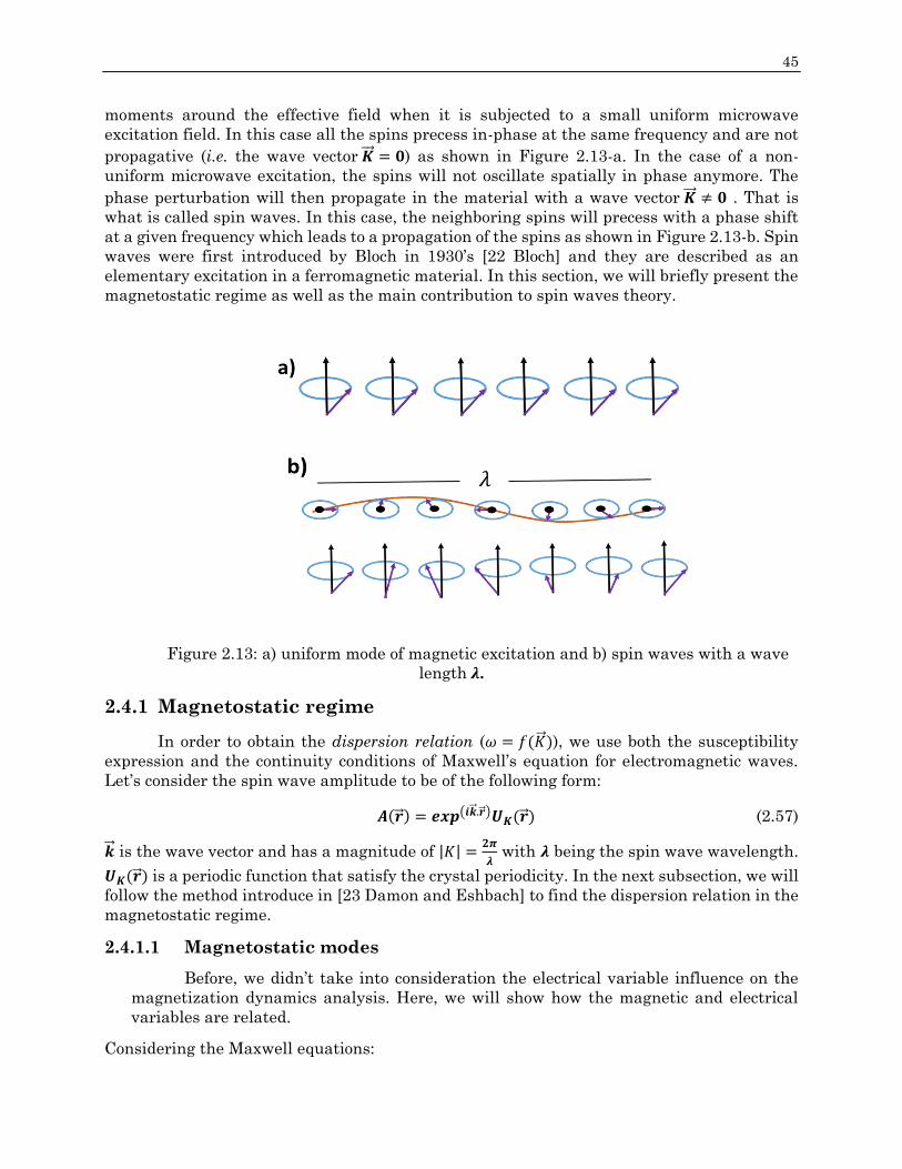
45
moments around the effective field when it is subjected to a small uniform microwave
excitation field. In this case all the spins precess in-phase at the same frequency and are not
propagative (i.e. the wave vector = 𝟎) as shown in Figure 2.13-a. In the case of a non-
uniform microwave excitation, the spins will not oscillate spatially in phase anymore. The
phase perturbation will then propagate in the material with a wave vector ≠ 𝟎 . That is
what is called spin waves. In this case, the neighboring spins will precess with a phase shift
at a given frequency which leads to a propagation of the spins as shown in Figure 2.13-b. Spin
waves were first introduced by Bloch in 1930’s [22 Bloch] and they are described as an
elementary excitation in a ferromagnetic material. In this section, we will briefly present the
magnetostatic regime as well as the main contribution to spin waves theory.
Figure 2.13: a) uniform mode of magnetic excitation and b) spin waves with a wave
length 𝝀.
2.4.1 Magnetostatic regime
In order to obtain the dispersion relation (𝜔 = 𝑓()), we use both the susceptibility
expression and the continuity conditions of Maxwell’s equation for electromagnetic waves.
Let’s consider the spin wave amplitude to be of the following form:
𝑨() = 𝒆𝒙𝒑(𝒊.)𝑼𝑲() (2.57)
is the wave vector and has a magnitude of |𝐾| =𝟐𝝅
𝝀 with 𝝀 being the spin wave wavelength.
𝑼𝑲() is a periodic function that satisfy the crystal periodicity. In the next subsection, we will
follow the method introduce in [23 Damon and Eshbach] to find the dispersion relation in the
magnetostatic regime.
2.4.1.1 Magnetostatic modes
Before, we didn’t take into consideration the electrical variable influence on the
magnetization dynamics analysis. Here, we will show how the magnetic and electrical
variables are related.
Considering the Maxwell equations:

46 Chapter 2: Magnetization dynamics
∧ =
𝝏
𝝏𝒕+
∧ = −𝝏
𝝏𝒕
. = 𝝆
𝜵 . = 𝟎
(2.58)
Where, is the magnetic field in (A/m), is the electric displacement in (C/m2), is the
electric current density in (A/m2), is the electric field in (V/m), 𝝆 is the electric charge density
in (C/m3) and is the magnetic induction field in (T). is related to the magnetic field and
polder tensor by the following relation:
= 𝝁𝟎( + ) = 𝝁𝟎( + ) = (2.59)
Where an identity matrix and µ is the permeability. + can be expressed, after the Polder
tensor derived in equation (2.31), as follows:
+ = = 𝝁𝟎 [𝟏 + 𝝌 −𝒊𝒌 𝟎
𝒊𝜿 𝟏 + 𝝌𝟎
𝟎 𝟎𝟏] (2.60)
The electric displacement and the current density are related to electric field by the following
formula:
= 𝝐
= 𝝈 (2.61)
𝝐 is the permittivity and 𝝈 is the electrical conductivity.
Let us consider that the different electrical and magnetic fields have a spatial and time
dependent function of the form 𝒆𝒙𝒑𝒊(.−𝝎𝒕), Maxwell’s equations can thus be written in the
following form:
𝒊 ∧ = −𝒊𝝎 +
∧ = −𝝎
𝒊 . = 𝝆
. = 𝟎
(2.62)
By replacing equation (2.59) and (2.61) in the first two equations of (2.62) and crossing 𝑲 into
both sides, we get:
∧ ∧ = −𝝎𝟐𝝐𝝁𝟎( + ) − 𝒊𝝎𝝈 𝝁𝟎( + ) (2.63)
Equation (2.62) can be simplified as follows:
∧ ∧ = −𝒌𝟎𝟐( + ) (2.64)
With,
𝒌𝟎𝟐 = 𝝎𝟐𝝁𝟎(𝝐 +
𝒊𝝈
𝝎) (2.65)

47
Expression (2.65) refers to the wave number for a propagating wave in a non-magnetic
medium. If 𝝐 ≫ 𝝈/𝝎, then the material is said to be dielectric with a wave number 𝒌𝟎 = 𝝎/𝒄, with 𝒄 is the speed of light. Whereas, if 𝝐 ≪ 𝝈/𝝎, the material behaves as a metal.
From equation (2.64), we can calculate the norm of curl as follows:
| ∧ | = | ∧ | =|∧∧|
||=𝒌𝟎
𝟐
𝐾|( + )| (2.66)
From the previous equation, we note that for high values of 𝐾 such that 𝑲 ≫ 𝒌𝟎, curl → 𝟎.
This approximation is called the magnetostatic approximation. In this case the magnetic and
electric part are not coupled anymore. Maxwell’s equations can then be written as:
∧ = 𝟎
∧ = 𝒊𝝎 𝒃
𝜵 . = 𝟎
(2.67)
, , and are the time dependent dynamic components of , , and , respectively.
As curl h = 0 we can define a magnetostatic potential 𝝍 such as: = −𝝍
Then 𝜵 . can be expressed as follows:
𝜵 . = 𝜵 (( + )𝝍) = 𝟎 (2.68)
From equation (2.68) and assuming that 𝝌 and 𝒌 are independent on position, we deduce the
following:
(𝑰 + 𝝌) [𝝏𝟐𝝍
𝝏𝒙𝟐+𝝏𝟐𝝍
𝝏𝒚𝟐] +
𝝏𝟐𝝍
𝝏𝒛𝟐= 𝟎 (2.69)
The previous equation is called the Walker’s equation [24 Walker] and its solutions are
referred to as the magnetostatic modes.
If we consider that the magnetostatic potential 𝝍 can be written in the form of 𝒆𝒙𝒑(𝒊 𝑲.), walker equation becomes:
(𝑰 + 𝝌)[𝒌𝒙𝟐 + 𝒌𝒚
𝟐] + 𝒌𝒛𝟐 = 𝟎 (2.70)
Equation (2.70) clearly connects the wave vector 𝒌 to the frequency (𝜔) in 𝝌.
Now if we consider that the magnetic field is applied along Z-axis (the direction of external
magnetic field), and the spin wave propagate with angle 𝜽 with respect to Z axis. Here we
consider an infinite medium Equation (2.70) becomes:
𝒌𝒙
𝟐 + 𝒌𝒚𝟐 = 𝒌𝟐 𝐬𝐢𝐧𝟐 𝜽
𝒌𝒛𝟐 = 𝒌𝟐 𝐜𝐨𝐬𝟐 𝜽
(2.71)
Substituting equation (2.71) in (2.70) yields to:
𝝌𝐬𝐢𝐧𝟐 𝜽 = −𝟏 (2.72)

48 Chapter 2: Magnetization dynamics
This can be expressed in terms of frequency using equation (2.32) for 𝝌. This gives the
following:
𝝌 𝐬𝐢𝐧𝟐 𝜽 =𝝎𝟎𝝎𝑴 𝐬𝐢𝐧
𝟐 𝜽
𝝎𝟎𝟐 −𝝎𝟐
(2.73)
Simplifying equation (2.73), we get:
𝝎 = [𝝎𝟎(𝝎𝟎 +𝝎𝑴 𝐬𝐢𝐧𝟐 𝜽)]
𝟏/𝟐 (2.74)
We notice that equation (2.74) is independent of the wave vector 𝒌. This is valid for an infinite
medium. The correspondence between 𝝎 and 𝒌 will be found by applying the boundary
conditions in the Maxwell equation. However, important comments can already be stated
from 2.74. Indeed, the frequency of the spin waves depends on the propagation direction θ.
We deduce that the resonance frequency is bounded between the two values [3 Stancil and
Prabhakar]:
𝝎𝟎 ≤ 𝝎 ≤ [𝝎𝟎(𝝎𝟎 +𝝎𝑴)]𝟏/𝟐 (2.75)
The previous band of frequencies is called ‘spin wave manifold’.
In thin films, the magnetostatic modes are determined by the direction of the wave vector, 𝒌,
with respect to the applied external field in-plane or out-of-plane.
We are now interested in solving Walker’s equation (2.69) to obtain the dispersion
relation for magnetostatic spin waves propagating normally or tangentially in magnetized
thin films. This leads us to the three principal configurations of magnetostatic waves in thin
films, presented as follows:
2.4.1.1.1 Magnetostatic Forward Volume Wave (MSFVW):
In this case, the magnetic external field is applied perpendicular to the surface plane
of the material and the magnetization, is oriented out-of-plane (𝑴 𝑯𝟎 ). If we have a
propagative spin wave vector in the plane of the film such that ((𝑴 𝑯𝟎 ) ⊥ 𝒌 ), then this
configuration is known as the MSFVW.
For spin waves propagating in a thin film with a wave vector; 𝒌 = 𝒕 + 𝒛 and 𝒕 = 𝒙 + 𝒚;
Kalinikos derived an explicit dispersion relation of the frequency 𝝎 for the lowest order 𝒏 = 𝟎
, where 𝒏 is the stationary condition inside the film’s thickness [25 Kalinikos]. The dispersion
relation is then written as follows:
𝝎𝟐 = 𝝎𝟎[𝝎𝟎 +𝝎𝑴(𝟏 −𝟏−𝒆𝒙𝒑−𝒌𝒕𝒅
𝒌𝒕𝒅)] (2.76)
Where d is the thickness of the film.
2.4.1.1.2 Magneto static Backward Volume waves (MSBVW):
In this configuration the external magnetic field is applied parallel to the sample’s
plane. The magnetization, is magnetized in-plane and the wave vector propagates in such
a way that ((𝑴 𝒌 ). This configuration is called MSBVW.

49
The propagation spin wave vector this time has the form of = 𝒕 + 𝒚 with 𝒕 = 𝒛. Kalinikos
also derived an explicit form of the dispersion relation for lowest order mode (fundamental
mode) 𝒏 = 𝟏:
𝝎𝟐 = 𝝎𝟎[𝝎𝟎 +𝝎𝑴(𝟏−𝒆𝒙𝒑−𝒌𝒛𝒅
𝒌𝒛𝒅)] (2.77)
Then, the phase and group velocities of MSBVW propagate in opposite direction.
2.4.1.1.3 Magnetostatic Surface Wave (MSSW):
We consider in this case that the propagating waves are perpendicular to an in-plane
external magnetic field such that ( ⊥ ). This configuration is called the MSSW or the
Damon-Eshbach mode [23 Damon and Eshbach]. The dispersion relation for MSSW is derived
by solving the Walker’s equation and is written as:
𝝎𝟐 = 𝝎𝟎(𝝎𝟎 +𝝎𝑴) +𝝎𝑴
𝟐
𝟒[𝟏 − 𝒆𝒙𝒑−𝟐𝒌𝒅] (2.78)
Similarly to MSBVW this dispersion relation of MSSW clearly depends on the thickness of
the magnetic film 𝑑 and on the magnitude of the wave vector. One of the most important
feature of MSSW is their evanescent character in the thickness of the film. This is why they
are called surface waves. This also implies that depending on the direction of with respect
to 𝑀, the wave will propagate on the upper or lower surface of the material. Finally, MSSW
have group and phase velocities propagating in the same direction.
The graphical presentation of all three magnetostatic waves is presented in Figure 2.14.
Figure 2.14: Topology of spin wave modes in a magnetic film as a function of the direction of
magnetization and the in-plane wave vector [26 Demokritov].
2.4.2 Spin waves in the exchange regime
We are now interested in solving the dispersion relation (2.78) taking into account the
exchange interaction term.

50 Chapter 2: Magnetization dynamics
Starting from equation (2.9), the operator ∇2 could be replaced by −𝒌𝟐. Then it is possible to
replace the resonance frequency 𝝎𝟎 by 𝝎𝟎 + 𝜸𝟐𝑨
𝑴𝒔𝒌𝟐 . The dispersion relation thus becomes:
𝝎𝟐 = (𝝎𝟎 + 𝜸𝟐𝑨
𝑴𝒔𝒌𝟐) + (𝝎𝟎 +𝝎𝑴 𝐬𝐢𝐧
𝟐 𝜽 + 𝜸𝟐𝑨
𝑴𝒔𝒌𝟐) (2.79)
Rado and Weertman [27 Rado & Weertman] have studied the modification of the spin waves
ferromagnetic resonance due to the influence of exchange interaction. The exchange
interaction is assumed to be at the interface of the magnetic layer where a surface uniaxial
anisotropy exist. In this configuration, boundary condition are taken into account at the
interface of the layer in addition to the electromagnetic ones in order to solve the equation of
motion. Soohoo et al. have proposed a general exchange boundary conditions in their paper
[28 Soohoo] such that:
𝝏𝒎𝒙
𝝏𝒛+ 𝒑 𝒎𝒙 𝐜𝐨𝐬(𝟐𝜽) = 𝟎 𝒂𝒏𝒅
𝝏𝒎𝒚
𝝏𝒛+ 𝒑 𝒎𝒚 𝐜𝐨𝐬
𝟐 𝜽 = 𝟎 (2.80)
𝒑 is the pinning factor and corresponds to the spin states at the interface. The condition 𝒑=0
represents the free spins. A perfect pinning corresponds to 𝒑 → ∞, which means that there is
a complete blockage of spins at the interface [29 Kittel].
2.4.2.1 Standing Spin waves (SSW)
Standing Spin waves (SSW) were first predicted theoretically by Kittel [29 Kittel] and
were first experimentally demonstrated by Seavey and Tannendwald [30 Seavey and
Tannendwald]. SSW belongs to the stationary family of magnetostatic modes. The wave
vector of SSW is parallel to the normal of the film. These waves undergo reflections at the
interfaces leading to a stationary state. This state depends on the thickness of the layer "𝒅" and pinning conditions. Using condition (2.80), we can solve for kz the two pinning parameters
at each interface as follows:
𝐜𝐨𝐭 𝒌𝒛𝒅 =𝒌𝒛𝟐−𝒑𝟏𝒑𝟐
𝒌𝒛(𝒑𝟏𝒑𝟐) (2.81)
Where 𝒑𝟏 and 𝒑𝟐 are the pinning factors at the two films surfaces. If 𝒑𝟏 = 𝒑𝟐 = 𝒑, expression
(2.81) becomes:
𝐜𝐨𝐭 (
𝒌𝒛𝒅
𝟐) =
𝒌𝒛
𝒑
−𝐭𝐚𝐧 (𝒌𝒛𝒅
𝟐) =
𝒌𝒛
𝒑
(2.82)
From equation (2.79), if we consider only the exchange term into account, then the resonance
frequency becomes:
𝝎𝒏 = 𝝎𝟎 −𝝎𝑴 + 𝜸𝟐𝑨
𝑴𝒔𝒌𝒛 𝒏𝟐 (2.83)
Equation (2.83) corresponds to the case when magnetization is out of plane. 2,nzk (For n=1, 2,
3 …) is the solution for the two equations in (2.82). Expression (2.83) can be written as:

51
𝝎𝒏 = 𝝁𝟎𝜸(𝑯𝟎 −𝑴𝒔 +𝟐𝑨
𝝁𝟎𝑴𝒔𝒌𝒛 𝒏𝟐 ) (2.84)
In the case of perfect pinning, dnk nz /, and if 0p dnk nz /1, , .
If we consider the magnetization in the plane of the film, then we get the resonance frequency
as:
𝝎𝒏𝟐 = (𝝎𝑴 +𝝎𝟎 + 𝜸
𝟐𝑨
𝝁𝟎𝑴𝒔𝒌𝒛 𝒏𝟐 )(𝝎𝟎 + 𝜸
𝟐𝑨
𝝁𝟎𝑴𝒔𝒌𝒛 𝒏𝟐 ) (2.85)
One major interest in the measurement of such standing spin waves modes that it gives access
to the exchange constant 𝑨 value.
2.5 Magnetization relaxation mechanism
In this section, we will focus on the different mechanisms that contribute to the intrinsic
and extrinsic relaxation processes of magnetization relaxation. The dissipative term in
equation (2.23) described by the phenomenological damping coefficient 𝜶, contains
contribution from both intrinsic and extrinsic relaxation mechanisms. Experimentally, 𝜶 is
measured through the line width of the magnetic susceptibility in equation (2.39). The
magnetization relaxation is governed by different energy dissipation mechanisms
summarized in Figure 2.15.
Figure 2.15: graphical presentation of the flow of energy from between the magnetic system
and other systems when RF field excites the uniform modes [4 Gurevich and Melkov].

52 Chapter 2: Magnetization dynamics
Relaxation processes, (energy dissipation), result from the energy distribution
between the magnetic excitations (magnons) and the crystal vibrations (phonons) or the
conduction electrons. Magnons-magnons relaxation is another relaxation mechanisms.
These processes are divided into two configurations: the spin-spin and spin-lattice relaxation
processes. The spin-spin relaxation processes can be caused by defects in the crystal [4
Gurevich and Melkov]. In most cases, the transferred energy to the lattice results in heating.
The spin-lattice relaxation is divided into two processes: First, the direct spin-lattice process
that is based on the direct energy transfer to the lattice upon the destruction of magnons and
the creation of phonons. Second, the indirect spin-lattice process that is based on the energy
transfer from magnons to the lattice by electron scattering.
In this section, we will present the basics of relaxation mechanisms in ferromagnets.
As this is a very complicated topic a complete description is above the goal of this manuscript.
For more details the reader is invited to refer to the references cited below.
2.5.1 Intrinsic relaxation processes
The intrinsic contribution to damping corresponds to the natural mechanisms allowing
dissipation of the energy in order that the magnetization gets back to its equilibrium position.
For example any precessing dipole radiates energy in free space and loses energy (radiation
losses). In ferromagnets, there are more efficient dissipative processes. Then we have two
main contributions, one corresponds to the relaxation of magnons by scattering with the
conduction electrons and the second one corresponds to direct coupling of the magnetic modes
with the phonons. We will also consider other mechanisms such as the dissipation due to eddy
current which is the most important relaxation in thick metallic sample.
Let’s note that there is no complete theory that describes the magnetic losses in
dynamic experiments. However, several models have been developed for ferromagnets since
the pioneering work of Kittel, Van Vleck or more recently by Heinrich or Kamberský [34-39].
Collision of magnons with itinerant electrons
In a metallic ferromagnet, the major source of damping is generally the electron-magnon
interaction. Two mechanisms arise depending if the spin of the conduction is conserved or
not. A very complete description of the different mechanisms can be found in [40 Woltersdorf].
1- s-d interaction: spin-flip scattering
Electron-magnon collision has been described by Berger in 1970’s [31 Berger] as the
collision of a magnon of energy 𝐸 = ℏ𝜔𝑞 with an itinerant electron of energy 𝜀𝐾 and spin state
𝜎 (𝜎 can be ±1
2). Figure 2.16 can be described as the creation and annihilation of electron-hole
pair as a result of the collision of magnons and itinerant electrons by s-d exchange interaction.
The itinerant electron is transferred to a higher energy defined as 𝜀𝑘+𝑞 with a spin state 𝜎′.
Due to the conservation of angular momentum, itinerant electron has to flip its spin when
coherently scattered by a magnon. If the electron hole pair undergoes a coherent scattering
event, with a phonon for example, a coherent magnon will be reemitted. This mechanism
leads to a renormalization of the landé g-factor [32 Heinrich]. The g-factor is related to both
electron hole pair excitation spin flip time 𝜏𝑠𝑓 and the momentum relaxation time 𝜏𝑚 as
follows:

53
𝜏𝑠𝑓
𝜏𝑚=
1
(𝑔−2)2 (2.86)
Where time 𝜏𝑠𝑓 is the electron hole pair excitation spin flip time and 𝜏𝑚 the momentum
relaxation time. Details of obtaining 𝜏𝑠𝑓 and 𝜏𝑚 can be found in [41 Dubois, 42 valet et Fert].
In the case where the electrons undergoes an incoherent scattering process (with a phonon or
a magnon), the dephasing of the reemitted magnons leads to an average loss of coherence and
then to damping. This process leads to a linear dependence of the linewidth with the
frequency, in agreement with a Gilbert like term and can be expressed as a function of the
density of states at fermi level Zf , the spin flip time and the square of the g-factor [43 Pelzl].
Where 𝜏 is the electron scattering time.
In half metals such events are not possible due to the full spin polarization. This
explains why the damping coefficient in these materials, such as Co2MnSi are much lower
than usual ferromagnetic (Fe, Ni, Co). However magnon-electron relaxation without spin flip
is still occurring.
𝛼𝑠−𝑑 = (𝛾ℏ2𝜋/𝜇0𝑀𝑠 )𝑍𝑓(𝑔 − 2)
2/𝜏 (2.87)
Figure 2.16: Collision between a Spin wave (a magnon) with energy ℏ𝜔𝑞 and an itinerant
electron with energy 𝜀𝐾 and spin state 𝜎 results in creation of an itinerant electron with
momentum 𝑘 + 𝑞 and spin orientation 𝜎′.
2- Spin-Orbit relaxation: non spin-flip scattering
Electron-magnon scattering without spin flip is due to the spin orbit interaction. This
effect has been described by Kamberský [33 Kamberský].
A classical representation of this effect is referred as the “breathing fermi surface”.
When the magnetization precesses, the Fermi surface has to be distorted periodically.
However such a repopulation of the energy levels for the electrons can be done only with a
timescale equal to momentum relaxation time Tm. Then a phase lag appears between the
precessing magnetization and the Fermi surface oscillations leading to a global loss of
coherence and then induces damping.

54 Chapter 2: Magnetization dynamics
Recent work by Kamberský [35, 36, 37 Kamberský] and Gilmore [44 Gilmore] based
on first principle calculations showed that the spin orbit relaxation is the dominant
mechanism in relaxation processes in ferromagnetic materials. In this model, the relaxation
rate is proportional to the spin-orbit coupling constant 𝜆𝑆𝑂 and the damping factor. The
corresponding damping coefficient is expressed as:
𝛼𝑆𝑂 = (𝛾ℏ𝜋/𝜇0𝑀𝑠)𝑍𝑓𝜆𝑆𝑂2 (𝑔 − 2)2 ∗ 𝜏 (2.88)
Following the approach of Kittel, the quantity (𝑔 − 2) can be expressed as the ratio of
the orbital to spin moment (𝑔 − 2 = 2 (𝜇𝐿
𝜇𝑠)). This is valid for small orbital moment but in
ferromagnet this is valid due to the quenching of the orbital by the crystal field. Then from
equation 2.88, we conclude that the Gilbert damping provides a sensitive probe of spin-orbit
effects and if there is any shift in the g-factor that is related to the spin-orbit coupling [43
Pelzl].
Intrinsic relaxation mechanisms induced by Eddy current
In thick metallic sample, a major source of relaxation comes from the eddy current
induced either by the oscillating pumping field or directly by the precessing magnetization
itself.
It is possible to demonstrate that they induce a component of the spin wave vector
perpendicular to the film surface. This additional wave vector is of the form 𝑘 = 1+i
√2𝜹 with 𝜹
the skin depth defined as:
𝜹 = √𝟐
𝝁𝝎𝝈 (2.89)
Where 𝜎 is the conductivity of any material and 𝜇 its permeability.
The imaginary part of the wave vector is responsible for the evanescence of the spin wave in
the thickness of the film and then to a loss of coherence. For samples thicker than the skin
depth 𝛅, the contribution of eddy current are taken into account by integrating Maxwell’s
equation across the film thickness d. The contribution of the eddy current to the damping can
be expressed as:
𝜶𝒆𝒅𝒅𝒚 =𝟏
𝟔𝑴𝒔𝜸 (
𝟒𝝅
𝒄)𝟐𝝈𝒅𝟐 (2.90)
Knowing the resistivity of CMS at room temperature to be 170 𝜇Ω𝑐𝑚 [10 Kämmerer], the skin
depth calculated at 10 GHz for CMS is in the range of 260 nm which is much bigger than our
studied CMS films (42 and 50 nm thickness layers). Thus, the contribution of eddy current
damping term, in our case, is negligible.
Magnon-phonon scattering
The direct coupling of magnons and phonons is another source of energy dissipation
for the precessing magnetization. A classical picture can be given as follows: let’s consider a
chain of spin localized on atoms. When a spin is precessing, the surrounding atoms will be
periodically either attracted or repealed due to the dipolar coupling between the spins, leading

55
to phonons. Reciprocally the propagating phonon will perturb the phase of the spin wave
leading to decoherence and consequently damping.
Detailed theories were developed by many groups but H. Suhl [45 Suhl] explicitly
presented the relaxation by a phonon drag that can be applied to small geometries with
homogeneous magnetization and lattice strain. The gilbert phonon damping is described as
follows:
𝜶𝒑𝒉𝒐𝒏𝒐𝒏 =𝟐𝜼𝜸
𝑴𝒔(𝑩𝟐(𝟏+𝝊)
𝑬)𝟐 (2.91)
Where 𝜼 is the phonon viscosity, B2 is the magneto-elastic shear constant, E is the
Young modulus and 𝝊 is the Poisson ratio.
Finally one could discuss about intrinsic magnon-magnon interaction that leads to
energy dissipation. These intrinsic mechanism are 3 and 4 magnons scattering. They have
been described by Suhl to explain nonlinear effects in spin dynamics experiments such as
additional absorption peaks or the saturation of the permeability.
The three magnon process, which is responsible for the subsidiary peak in high power
experiments, corresponds to the relaxation of a uniform magnon with 𝑘0 and energy 𝜔0 into
two magnons with opposite wave vectors +𝑘 and −𝑘 of energy ℏ𝜔0/2. The four magnon process
scattering corresponds to the annihilation of two magnons uniform modes with 𝑘0 and 𝜔0 into
two magnons with wave vector +𝑘 and −𝑘 and energy ℏ𝜔0. This is the source of the saturation
for the susceptibility.
However, these effects mainly arises for nonlinear excitation of the magnetization. In
our work, we only work in the small perturbation (linear) limit and then we will not discuss
these two mechanisms. The reader is invited to refer to [3, 4, 46, and 47] for more details.
2.5.2 Extrinsic relaxation processes
Another source of energy losses comes from structural defects, interface effects or
inhomogeneity of the magnetic parameters. In general such mechanisms are referred as
extrinsic contribution to the damping as they are related to imperfections of the ideal
material. Experimentally, the extrinsic contributions to the relaxation induce a non-zero
linewidth at zero frequency (∆𝑯𝟎).
Different parameters can contribute to these extrinsic processes. The principal source of
extrinsic relaxation is generally the two magnons scattering and the inhomogeneity of
magnetic parameters. They have been described for example in Zakeri et al. [52 Zakeri].
Inhomogeneity.
The inhomogeneity of magnetic parameters is a main source of damping in materials.
Indeed local variations of the effective field leads to the dephasing of the spins and then to
the decoherence of the precession.
The linewidth broadening due to magnetic inhomogeneity can be calculated via a
general formula:

56 Chapter 2: Magnetization dynamics
∆𝐻A = |𝜕𝐻𝑟𝑒𝑠
𝜕𝐴| ∆𝐴 (2.92)
Where ΔA is the average spread of a magnetic parameter of interest A, such as the
amplitude of the magnetization 𝑀𝑠 or anisotropy 𝐻𝑘. It can also correspond to the spreading
of the easy axis direction 𝜑𝐻 due to the mosaicity of the material. This case is generally
referred as ΔHmos. This last term is generally one of the most important sources of linewidth
broadening but vanishes for field applied parallel to easy and hard axis directions.
One of the most important feature of equation 2.92 is that the linewidth broadening
due to magnetic inhomogeneity is frequency and angle independent.
Two-magnon scattering
In the two magnon relaxation process, the uniform mode of precession (𝑘 = 0) is scattered
by a defect into a non-zero wave vector spin wave (𝑘 ≠ 0) with the same energy. Two main
points have to be mentioned here. First, the conservation of momentum is not required as
long as the impurity can absorb the difference of momentum. Secondly, one crucial point is
that the FMR mode has to be degenerated with a non-uniform mode. This implies a non-
monotonous shape of the dispersion curve as shown in Figure 2.17.
Figure 2.17: spin wave dispersion curves as a function of wave vector in the case of thin
films. The gray region represents the case of tangentially magnetized thin film while the
dashed line represents the case of a perpendicularly magnetized film [53 Bailleul].
Two magnon scattering is generally caused by geometrical defects, crystal defects or
boundaries, etc... It is given by the following expression [54 Arias and Mills]:
∆𝐻2 magnon = ∑ Γ𝑥𝑖 × arcsin [𝑓
√𝑓2+(𝑓0)2+𝑓0
]𝑥𝑖 (2.93)
With Γ𝑥𝑖 is the strength of the two –magnon scattering along the in-plane crystalline
direction 𝑥𝑖 , 𝑓0 = 𝛾𝑀𝑒𝑓𝑓, and 𝑀𝑒𝑓𝑓 = 𝑀𝑠 − 𝐻𝑘/4𝜋.

57
It is important to note that for perpendicular configuration, i.e. a magnetic field applied
perpendicular to the surface of the film, the dispersion relation shows no degenerate mode of
the uniform mode with non-zero wave vector spin waves as long as θ, the angle between the
magnetization and the normal of the surface is <45°. Experimentally, this gives a special
signature of the ΔH vs θ curve (figure 2.18) [48-51].
Figure 2.18: Angular dependence of linewidth ∆𝐻𝑝𝑝 of FMR spectra in out of-Plane geometry
for Co2MnSi film. Panels (a) and (b) respectively depict line-width variations versus out-of-
plane angle 𝜑𝐻 in the easy- and hard-axis directions [48 Yilgin].
After giving a brief description in this section about the intrinsic and extrinsic relaxation process of magnetization relaxation. A summery is given on the influence of these contribution on the magnetic parameters of the CMS Heusler alloys investigated in this manuscript. The CMS thin films being studied later on in chapters 4 and 5 have a thickness less than 100 nm, and as noted earlier in this section, the eddy current contribution to the intrinsic relaxation process is then negligible. Whereas the magnon phonon damping factor couldn’t be evaluated for CMS due to unknown parameters in literature such as the magneto-elastic shear constant, we will follow the assumption proposed by Kamberský stating that the damping of most of ferromagnetic material is due to electron-magnons scattering [37 Kamberský]. This leads the spin orbit interaction to be the dominant intrinsic contribution to relaxation mechanism where the damping factor depends on the spin orbit coupling through the relation 2.88.
The extrinsic relaxation processes are described by the frequency independent contribution to the linewidth. They are induced by crystal inhomogeneity such as defects, interface effects and magnetic inhomogeneity such as local variation of magnetization or anisotropy. Considering classical values of the extrinsic contributions to the linewidth observed in many studies on similar materials [49 Belmeguenai, 56 Qiao], the value of ΔH0 is generally about 10 Oe. In our CMS samples, slightly higher values of ΔH0 will be measured (see chapters 4 and 5). The most probable reason is a stronger contribution of the ∆𝑯𝒊𝒏𝒉𝒐𝒎𝒐𝒈𝒆𝒏𝒆𝒊𝒕𝒚 and ∆𝑯𝒎𝒐𝒔𝒂𝒊𝒄𝒊𝒕𝒚 as we will show that our samples have one or two crystal phase order as deposited. . Also 2 magnons scattering has probably a significant contribution to the linewidth, especially in our irradiated samples (chapter5) for which local defects are created at high fluence. However, this one is very difficult to estimate and requires

58 Chapter 2: Magnetization dynamics
high field in and out-of-plane FMR measurements, the latter being not accessible within our stet-up.
Chapter 2 References:
[1] J. M. D. Coey, Magnetism and magnetic materials. Cambridge; New York: Cambridge
University Press, 2009.
[2] S. Blundell, Magnetism in condensed matter, reprinted. Oxford: Oxford Univ. Press, 2003.
[3] D. Stancil and A. Prabhakar, Spin Waves. Boston, MA: Springer US, 2009.
[4] Guervich and Merkov, “Magnetization Oscillations and Waves,”
[5] S. V. Vonsovskii, Ferromagnetic resonance: the phenomenon of resonant absorption of a
high-frequency magnetic field in ferromagnetic substances, vol. 4. Elsevier, 2013.
[6] M. Getzlaff, Fundamentals of magnetism. Berlin ; New York: Springer, 2008.
[7] M. A. Ruderman and C. Kittel, “Indirect exchange coupling of nuclear magnetic moments
by conduction electrons,” Phys. Rev., vol. 96, no. 1, p. 99, 1954.
[8] T. Kasuya, “A theory of metallic ferro-and antiferromagnetism on Zener’s model,” Prog.
Theor. Phys., vol. 16, no. 1, pp. 45–57, 1956.
[9] K. Yosida, “Magnetic Properties of Cu-Mn Alloys,” Phys. Rev., vol. 106, no. 5, pp. 893–
898, juin 1957.
[10] S. Kämmerer, S. Heitmann, D. Meyners, D. Sudfeld, A. Thomas, A. Hütten, et G. Reiss,
« Room-temperature preparation and magnetic behavior of Co2MnSi thin films », J. Appl.
Phys., vol. 93, no 10, p. 7945, 2003..
[11] U. Falk, A. Furrer, J. K. Kjems, and H. U. Güdel, “Biquadratic Exchange in Cs Mn x
Mg 1- x Br 3,” Phys. Rev. Lett., vol. 52, no. 15, p. 1336, 1984.
[12] N. L. Huang and R. Orbach, “Biquadratic Superexchange,” Phys. Rev. Lett., vol. 12, no.
11, pp. 275–276, Mar. 1964.
[13] I. Dzyaloshinsky, “A thermodynamic theory of ‘weak’ ferromagnetism of
antiferromagnetics,” J. Phys. Chem. Solids, vol. 4, no. 4, pp. 241–255, 1958.
[14] T. Moriya, “Anisotropic superexchange interaction and weak ferromagnetism,” Phys.
Rev., vol. 120, no. 1, p. 91, 1960.
[15] J. H. van Vleck, “On the anisotropy of cubic ferromagnetic crystals,” Phys. Rev., vol.
52, no. 11, p. 1178, 1937.
[16] L. D. Landau and E. Lifshitz, “On the theory of the dispersion of magnetic permeability
in ferromagnetic bodies,” Phys Z Sowjetunion, vol. 8, no. 153, pp. 101–114, 1935.
[17] N. Bloembergen, “On the ferromagnetic resonance in nickel and supermalloy,” Phys.
Rev., vol. 78, no. 5, p. 572, 1950.
[18] T. L. Gilbert and H. Ekstein, “Basis of the domain structure variational principle,”
Bull. Amer. Phys. Soc., vol. 1, p. 25, 1956, and T. L. Gilbert, “A phenomenological theory
of damping in ferromagnetic materials,” IEEE Trans. Magn., vol. 40, no. 6, pp. 3443–3449,
Nov. 2004.
[19] G. Ortiz, A. Garcia-Garcia, N. Biziere, F. Boust, J. F. Bobo, and E. Snoeck, “Growth,
structural, and magnetic characterization of epitaxial Co2MnSi films deposited on MgO
and Cr seed layers,” J. Appl. Phys., vol. 113, no. 4, p. 043921, 2013.
[20] Smit, J. and H.G. Belgers, Ferromagnetic resonance absorption in BaFe12O19, a
highlyanisotropic crystal. Philips Res. Rep., 1955. 10: p. 113-30.
[21] Suhl, H., “Theory of the magnetic damping constant”, IEEE Trans. Magn. 34, 1834
(1998).

59
[22] F. Bloch, “Zur theorie des austauschproblems und der remanenzerscheinung der
ferromagnetika,” Z. Für Phys., vol. 74, no. 5–6, pp. 295–335, 1932.
[23] R. W. Damon and J. R. Eshbach, “Magnetostatic modes of a ferromagnet slab,” J. Phys.
Chem. Solids, vol. 19, no. 3, pp. 308–320, mai 1961.
[24] L. R. Walker, “Magnetostatic Modes in Ferromagnetic Resonance,” Phys. Rev., vol.
105, no. 2, pp. 390–399, Jan. 1957.
[25] B. A. Kalinikos, “Excitation of propagating spin waves in ferromagnetic films,”
Microw. Opt. Antennas IEE Proc. H, vol. 127, no. 1, p. 4, 1980.
[26] S. O. Demokritov, B. Hillebrands, and A. N. Slavin, “Brillouin light scattering studies
of confined spin waves: linear and nonlinear confinement,” Phys. Rep., vol. 348, no. 6, pp.
441–489, 2001.
[27] G. T. Rado and J. R. Weertman, “Spin-wave resonance in a ferromagnetic metal,” J.
Phys. Chem. Solids, vol. 11, no. 3, pp. 315–333, Oct. 1959.
[28] R. F. Soohoo, “General exchange boundary condition and surface anisotropy energy of
a ferromagnet,” Phys. Rev., vol. 131, no. 2, p. 594, 1963.
[29] C. Kittel, “Excitation of spin waves in a ferromagnet by a uniform rf field,” Phys. Rev.,
vol. 110, no. 6, p. 1295, 1958.
[30] M. H. Seavey Jr and P. E. Tannenwald, “Direct observation of spin-wave resonance,”
Phys. Rev. Lett., vol. 1, no. 5, p. 168, 1958.
[31] L. Berger, “A simple theory of spin-wave relaxation in ferromagnetic metals,” J. Phys.
Chem. Solids, vol. 38, no. 12, pp. 1321–1326, Jan. 1977.
[32] B. Heinrich, D. Fraitová, and V. Kamberský, “The Influence of s-d Exchange on
Relaxation of Magnons in Metals,” Phys. Status Solidi B, vol. 23, no. 2, pp. 501–507, Jan.
1967.
[33] V. Kamberský, “On the Landau–Lifshitz relaxation in ferromagnetic metals,” Can. J.
Phys., vol. 48, no. 24, pp. 2906–2911, décembre 1970.
[34] V. Kamberskỳ, “On ferromagnetic resonance damping in metals,” Czechoslov. J. Phys.
B, vol. 26, no. 12, pp. 1366–1383, 1976.
[35] V. Kamberskỳ, “Dissipative boundary conditions for ferromagnetic resonance
equations,” Czechoslov. J. Phys. B, vol. 23, no. 6, pp. 627–635, 1973.
[36] V. Kamberskỳ, “FMR linewidth and disorder in metals,” Czechoslov. J. Phys., vol. 34,
no. 10, pp. 1111–1124, 1984.
[37] V. Kamberský, “Spin-orbital Gilbert damping in common magnetic metals,” Phys. Rev.
B, vol. 76, no. 13, Oct. 2007
[38] B. Heinrich, J. F. Cochran, and R. Hasegawa, “FMR linebroadening in metals due to
two‐magnon scattering,” J. Appl. Phys., vol. 57, no. 8, pp. 3690–3692, Apr. 1985.
[39] B. Heinrich, G. Woltersdorf, R. Urban, and E. Simanek, “Role of dynamic exchange
coupling in magnetic relaxations of metallic multilayer films (invited),” J. Appl. Phys., vol.
93, no. 10, p. 7545, 2003.
[40] G. Woltersdorf, “Spin-pumping and two-magnon scattering in magnetic multilayers,”
Sinon Fraser University, 2004.
[41] S. Dubois, L. Piraux, J. M. George, K. Ounadjela, J. L. Duvail, and A. Fert. Evidence
for a short spin diffusion length in permalloy from the giant magnetoresistance of
multilayered nanowires. Phys. Rev. B, 60:477–484, 1999.
[42] T. Valet and A. Fert. Theory of the perpendicular magnetoresistance in magnetic
multilayers. Phys. Rev. B, 48:7099–7113, 1993.

60 Chapter 2: Magnetization dynamics
[43] J. Pelzl, R. Meckenstock, D. Spoddig, F. Schreiber, J. Pflaum, and Z. Frait, “Spin–
orbit-coupling effects on g-value and damping factor of the ferromagnetic resonance in Co
and Fe films,” J. Phys. Condens. Matter, vol. 15, no. 5, p. S451, 2003.
[44] H. Keith Gilmore, “Gas sensors based on conducting polymers,” Sensors, vol. 7, no. 3,
pp. 267–307, 2007.
[45] H. Suhl, The theory of ferromagnetic resonance at high signal powers, J. Phys. Chem.
Solids, 1 (1957), p. 209.
[46] J. T. Łopuszański, A. Pękalski, and J. Przystawa, Eds., Magnetism in Metals and
Metallic Compounds. Boston, MA: Springer US, 1976.
[47] R. A. Lukaszew, Handbook of Nanomagnetism: Applications and Tools. CRC Press,
2015.
[48] R. Yilgin, Y. Sakuraba, M. Oogane, S. Mizukami, Y. Ando, and T. Miyazaki,
“Anisotropic Intrinsic Damping Constant of Epitaxial Co2MnSi Heusler Alloy Films,” Jpn.
J. Appl. Phys., vol. 46, no. 9, pp. L205–L208, 2007.
[49] M. Belmeguenai, H. Tuzcuoglu, M. S. Gabor, T. Petrisor, C. Tiusan, D. Berling, F.
Zighem, T. Chauveau, S. M. Chérif, and P. Moch, “Co2FeAl thin films grown on MgO
substrates: Correlation between static, dynamic, and structural properties,” Phys. Rev. B,
vol. 87, no. 18, p. 184431, mai 2013.
[50] H. Kurebayashi, T. D. Skinner, K. Khazen, K. Olejník, D. Fang, C. Ciccarelli, R. P.
Campion, B. L. Gallagher, L. Fleet, A. Hirohata, and A. J. Ferguson, “Uniaxial anisotropy
of two-magnon scattering in an ultrathin epitaxial Fe layer on GaAs,” Appl. Phys. Lett.,
vol. 102, no. 6, p. 062415, 2013.
[51] H.-S. Song, K.-D. Lee, J.-W. Sohn, S.-H. Yang, S. S. P. Parkin, C.-Y. You, and S.-C.
Shin, “Relationship between Gilbert damping and magneto-crystalline anisotropy in a Ti-
buffered Co/Ni multilayer system,” Appl. Phys. Lett., vol. 103, no. 2, p. 022406, 2013.
[52] K. Zakeri, J. Lindner, I. Barsukov, R. Meckenstock, M. Farle, U. von Hörsten, H.
Wende, W. Keune, J. Rocker, S. Kalarickal, K. Lenz, W. Kuch, K. Baberschke, and Z.
Frait, “Spin dynamics in ferromagnets: Gilbert damping and two-magnon scattering,”
Phys. Rev. B, vol. 76, no. 10, Sep. 2007.
[53] M. Bailleul, Propagation et con_nement d'ondes de spin dans les microstructures
magnétiques, Thèse de doctorat de l'Ecole Polytechnique,2002.
[54] R. Arias and D. L. Mills, “Extrinsic contributions to the ferromagnetic resonance
response of ultrathin films,” Phys. Rev. B, vol. 60, no. 10, pp. 7395–7409, Sep. 1999.
[55] S.-Z. Qiao, J. Zhang, Y.-F. Qin, R.-R. Hao, H. Zhong, D.-P. Zhu, Y. Kang, S.-S. Kang,
S.-Y. Yu, G.-B. Han, S.-S. Yan, and L.-M. Mei, “Structural and Magnetic Properties of Co
2 MnSi Thin Film with a Low Damping Constant,” Chin. Phys. Lett., vol. 32, no. 5, p.
057601, May 2015.

61
Chapter 3: Experimental
techniques
In this chapter, we will introduce the different techniques used to study the structural
and magnetic properties of ‘as deposited’ Co2MnSi (CMS) Heusler alloy. Section 3.1 describes
different deposition technique. In section 3.2 thin film deposition procedure of CMS will be
presented. Section 3.3 the structural investigation by X-Ray Diffraction (XRD) and
Transmission Electron Microscopy (TEM) is carried on the deposited CMS thin films. In
section 3.4 Magneto Optical Kerr Effect (MOKE) and Ferromagnetic Resonance (FMR)
spectroscopy experiments are used to study the static and dynamic magnetic properties of
CMS. At the end of this chapter, Ion irradiation technique is introduced.
3.1 Deposition Techniques
Thin films fabrication are usually divided into two categories, the Chemical Vapor
Deposition (CVD) and the Physical Vapor Deposition (PVD). In CVD process, the material to
be deposited is in the gas or liquid form, the deposition is done by a chemical reaction on the
substrate surface. While, PVD technique is based on the formation of a vapor state of the
material to be deposited as thin films onto the substrate. To convert the material from solid
to vapor state, is done by either thermal evaporation (i.e. heating) or sputtered/bombarded
ions.
PVD by thermal evaporation:
It is one of the oldest methods to deposit thin films, metals are evaporated by heating and
the evaporated material will form a thin layer on the used substrate. The ultra-high vacuum
is necessary for film deposition (< 10-8 Torr). Thermal evaporation can be divided into two
parts: Filament evaporation and Electron-beam one. Filament evaporation is done by placing
the desired metal on the filament directly (usually Tungsten, W), then the metal is evaporated
as we increase the temperature of the filament. The rate of deposition is directly related to
the temperature of the filament and it should be lower than the sublimation temperature to
avoid contamination. In the case of electron-beam evaporation, electron beam is focused on
the material to evaporate instead of heating it. Different techniques are used to elaborate thin
films by evaporation, such as: Molecular Bean Epitaxy (MBE) and Pulsed laser deposition
(PLD). The reader is invited to refer to [1,2,3,4 and 5] for more details about PLD and MBE.

62 Chapter 3: Experimental techniques
PVD by ionic bombardment:
In this technique, ionic bombardment attack the material to be deposited (called
target) and ejects the atoms from its surface. There exist two ways of ionic bombardment:
either by direct application of ion beam on the target or by accelerated ionized gas (usually
Argon Gas) that release the atoms from the target placed at a cathode, results in creating a
plasma. An example of the former technique is Ion Beam Deposition (IBD) and the latter is
the sputtering. Sputtering is the VPD technique used for elaborating CMS thin films and is
detailed in the next paragraph.
3.1.1 Sputtering
This technique is used to deposit thin films by the creation of a gaseous plasma. The
ionized gas in the plasma accelerate towards the target (the material to be deposited). Atoms
are ejected from the target after being eroded by the energy transfer of the accelerating ions.
After being ejected, the atoms will be deposited on a nearby surface (the substrate). The
ionized gas used in our case is Argon, Ar. The use of neutral gas will avoid chemical reaction
with the deposited material. Apart from the use of Argon to deposit metals and alloys, Oxygen
ionized gas is used to deposit oxides. Compared to MBE (deposition rate of nm/hr), the rate
of deposition of sputtering is higher and of order of one atomic layer per second. In this work
we use face to face configuration for the CMS target in order to keep the stoichiometry of the
material when it is deposited on the substrate. Now, we will present the different energy
sources configurations to maintain the gaseous plasma.
DC configuration
In the DC configuration of sputtering, the target is inside the vacuum chamber of ~
10-7 mbar. Two electrodes are located inside the chamber to create the plasma. The target is
fixed on the first negatively charged electrode (cathode) that carries a negative potential
ranges from several volts to kilovolts. The second electrode (the anode) is placed on the
substrate, placed at few centimeters from the target. To create the plasma, we introduce the
Argon gas of 10-4 to 10-1 mbar, then, the free electrons will accelerate from the cathode and
approach the outer shell electrons of the Ar atoms, this leaves the Ar atoms electrically
unbalanced and forms ions instead, Ar+ ions. The positively charged ions will interact with
the atoms on the negatively charged electrode (the cathode) leading to an energy transfer
from the ions to free electrons and atoms of the target. The atoms will be deposited on the
substrate while the free electrons will hit the outer electron shells of Ar+ ions, changing them
into neutral gas. Due to the conservation of energy law, the Ar gas atoms that gained energy
must be released, the released energy is in the form of photons. For this reason we see the
glowing plasma (Figure 3.1).

63
Figure 3.1: Graphical representation of sputtering configuration.
RF configuration
The DC configuration is adapted to deposit conducting materials but it is not
applicable to deposit dielectrics or oxides. The reason falls behind is that Ar+ ions accumulate
on the target surface and the electrons coming from the cathode can’t neutralize the dielectric
materials. To overcome this problem, both electrodes should be polarized by an alternating
radio frequency (RF) potential. This leads to attract the electrons or the positive ions who
discharged the surface. The RF operating at frequencies higher than 1 MHz, is sufficient for
the positive ions to reach the electrodes. Usually, the used frequency is about 13.5 MHz to
avoid interference with telecommunication waves.
Face to Face configuration
Face to face configuration involves placing the two targets electrodes facing each other
separated by few centimeters where the substrate is placed above them (Figure3.2). In this
configuration, the two target electrodes are biased by RF potential. This configuration lower
the deposition rates and the probability of high energy carbon contamination is reduced.
Those two consequences of face to face target configuration allows us to have an epitaxial
growth from stoichiometry targets. The stoichiometry of the targets can be only reserved by
using the face to face configuration. In this thesis, face to face configuration is used to grow
the Co2MnSi Heusler alloys and MgO layers.
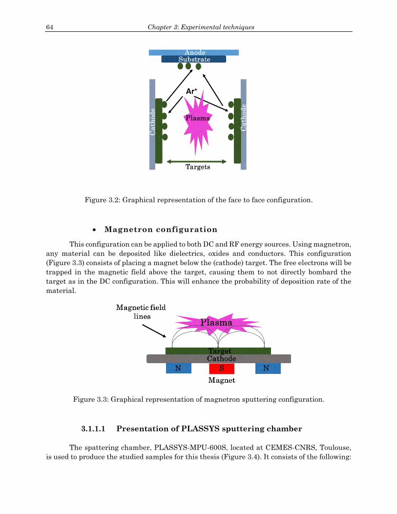
64 Chapter 3: Experimental techniques
Figure 3.2: Graphical representation of the face to face configuration.
Magnetron configuration
This configuration can be applied to both DC and RF energy sources. Using magnetron,
any material can be deposited like dielectrics, oxides and conductors. This configuration
(Figure 3.3) consists of placing a magnet below the (cathode) target. The free electrons will be
trapped in the magnetic field above the target, causing them to not directly bombard the
target as in the DC configuration. This will enhance the probability of deposition rate of the
material.
Figure 3.3: Graphical representation of magnetron sputtering configuration.
3.1.1.1 Presentation of PLASSYS sputtering chamber
The spattering chamber, PLASSYS-MPU-600S, located at CEMES-CNRS, Toulouse,
is used to produce the studied samples for this thesis (Figure 3.4). It consists of the following:

65
A cryogenic pump that ensures a high vacuum in the chamber (~10−8
mbar).
Load lock high vacuum chamber (~10−7 mbar), permits to transfer the
substrate inside the main chamber.
Substrate heater holder (up to 1000° C), rotates 360° degrees and can be
transferred from one position to another.
Two ‘face to face’ targets connected to an alternative RF potential and 3 DC
magnetron modes.
Two flow meters controls for Argon and Oxygen gas (Ar and O2).
An electron canon and florescent screen that enable us to control and verify
in-situ (during the growth procedure) the crystalline quality of the thin film
by Reflective High Energy Electron Diffraction (RHEED).
Figure 3.4: graphical representation of PLASSYS sputtering at CEMES.
3.2 CMS Thin film deposition procedure
In this section, we will present the different procedures to prepare CMS thin films starting
from the substrate choice, the buffer layer, the deposition condition of CMS thin films and the
last step by depositing a capping protection layer.
As presented in the first chapter, Heusler alloys can grow on different substrates and
by different deposition techniques. GaAs and MgO substrates are widely used for the
deposition of Heusler alloys. Although GaAs has a better mismatch for Heusler Co-based
alloys, MgO substrates take advantage over GaAs for Magnetic tunnel Junctions applications.
In our case, we use MgO substrates. CMS grows with a 45° angle rotation with respect to the
(100) MgO plane and a lattice mismatch of -5.4 %, enabling epitaxial growth.
66 Chapter 3: Experimental techniques
We use commercial monocrystalline MgO 10*10 or 20*20 mm3 mm2 epi-polished
substrates, provided by NEYCO. MgO substrates when introduced in the main chamber of
sputtering is annealing at 700° C for 1 hour to degas and reduce the roughness of the surface.
After annealing, a homo-epitaxial growth of MgO thin layer (~ 10 to 15 nm) is realized
to reduce the defects and to insure a 2D thin film epitaxial growth of CMS layers. As
mentioned in [6 Turban], a homo-epitaxial buffer layer blocks the diffusion of carbon atoms
towards the surface substrate and consequently reduces the defects to obtain a 2D surface
film for the epitaxial growth of CMS. MgO is deposited at 100° C using ‘the face to face’
configuration with a 100 Watts RF tension and a flow rate of 50 and 5.3 sccm for Ar and O2,
respectively. The MgO buffer layer surface was controlled by RHEED. RHEED images are
shown in Figure 3.8.
After the deposition of the homo-epitaxial MgO layer, CMS thin films are deposited
using also the face to face configuration. In this configuration the stoichiometry of the target
consists of 50% Co, 25% Mn and 25% Si. The plasma in this case is formed by Ar gas only.
The different depositions conditions (RF power of 100 w, Ar pressure flow of 50 sccm, CMS
deposition and annealing temperatures of 600 °c and 800 °, respectively) have been optimized
from the previous work of G. Ortiz [7 Ortiz].
The deposition rate is 1.5 nm/minute. In this work, the thickness of the CMS layer is
always about 40 nm. This value has been chosen to avoid He+ ions implantation during the
irradiation process (see section 3.5). One crucial point in deposition procedure to achieve high
crystalline CMS quality is the deposition and annealing temperature. The choice of the
deposition and annealing temperature will be presented in chapter IV.
At the end of the process, a few nanometers of capping layer of MgO is deposited to
prevent contamination and oxidation of the CMS layer when it is exposed to the normal
atmosphere conditions. Moreover, it is important for the ferromagnetic resonance experiment
to have a small insulating layer to avoid contact between the transmission line and the
metallic surface.
In this thesis, we have fabricated many samples following the above deposition conditions.
Among the different samples we had, even with the in-situ RHEED patterns verification, the
decision to proceed with magnetic and structural characterization was based on the lowest
peak to peak line width. Three samples have been selected and will be presented in the next
chapters. .
3.3 Structural characterization techniques
In this section, we will present the different experimental techniques used to investigate
the structural properties of CMS thin films. In this work, Reflection High Energy Electron
Diffraction (RHEED) was in-situ used during the deposition procedures to control the film
growth quality (2D vs 3D), normal and anomalous x-ray diffraction are used to define the
structure order of the film and the probability to define the atomic positions in the unit cell.
These characterization techniques have been correlated with Transmission Electron
Microscopy (TEM) techniques to study, on the Nano meter scale, the crystal deformation after
67
He+ irradiation using Geometric Phase Analysis (GPA) and direct observation of the local
order by HAADF STEM.
We first recall some diffraction basics to introduce RHEED, X-ray diffraction techniques
as well as describing the atomic disorder method used from x-ray diffraction peaks analysis.
Then, TEM, HAADF STEM imaging technique is introduced and GPA analysis method is
briefly described.
3.3.1 Basics of crystallography diffraction
By structural characterization, we study the topology and morphology of the crystal
by sending beam of electrons or x-rays on the substrate surface. These methods vary from
millimeter to nanometer scale. In this section we recall the theory of diffracted x-rays or
electrons from a given surface for this, first we recall the crystallography basics of real and
reciprocal space.
A crystal lattice is a solid material whose constituents (atoms, ions or molecules) are
arranged in a highly ordered 3 dimensional periodic structure and symmetry. A unit cell is
smallest volume of a crystal and defined by three neighboring atom unit vectors , and 𝑐 in
the x,y and z axes, respectively. Atoms in the crystal can be defined as a point in the real pace
lattice as 𝑇 = 𝑢 + 𝑣 + 𝑤𝑐, with [𝑢𝑣𝑤] is the real space direction integers.
For experimental techniques, we can’t have access to the real space components of a
crystal, but we can obtain a unit of inverse length. Thus, we define a reciprocal space lattice
that is related to the real space. The unit vectors in the reciprocal space have a reciprocal
relationship with the one of the real space by (ℎ𝑘𝑙) = ℎ ∗ + 𝑘∗ + 𝑙 𝑐∗, where ℎ, 𝑘 𝑎𝑛𝑑 𝑙 are
the miller indices of a plane (ℎ𝑘𝑙), and ∗, ∗ and 𝑐∗ are the reciprocal unit vectors, with
𝒂∗ = 𝟐𝝅𝒃∧𝒄
𝒂.(𝒃∧𝒄) , 𝒃∗ = 𝟐𝝅
𝒄∧𝒂
𝒂.(𝒃∧𝒄) and 𝒄∗ = 𝟐𝝅
𝒂∧𝒃
𝒂.(𝒃∧𝒄).
For diffraction experimental techniques, electrons or x-rays behave as matter waves
following the de Broglie relation 𝜆 = ℎ/𝑝 with 𝑝 =ℎ
2𝜋𝐾, where K is the wave vector expressed
as, 𝑘 = 2𝜋/𝜆. The diffraction of a wave requires an incoming wave vector KIN and a scattered
wave vector KOUT. Now we present how the wave vector can be diffracted using Bragg’s
relation and Ewald reconstruction.
Bragg’s Relation:
Bragg had announced that waves behave as if they are reflected from the atomic
planes and the wave vector K is related to the interplanar distance dhkl. In Figure 3.5, an
incoming vector incident on the first atomic plane with an angle 𝜃𝑖𝑛 is diffracted with an
angle 𝜃𝑜𝑢𝑡 = 𝜃𝑖𝑛 = 𝜃. If the same wave vector hits the surface and diffracted from the second
atomic plane, then the path length difference between the first and second ray is calculated
as: 2𝑑ℎ𝑘𝑙 sin 𝜃. If the path-length difference is of an integer wavelength form, then we get
Bragg’s law:
𝟐𝒅𝒉𝒌𝒍 𝐬𝐢𝐧𝜽 = 𝒏𝝀 (3.1)

68 Chapter 3: Experimental techniques
Figure 3.5: Schematic illustration of Bragg’s law.
Ewald sphere
Ewald construction defines the direction of the diffracted wave by an intersection of
two points. The first consists of incident wave vector with |𝐾𝑖𝑛| = 1/𝜆. The second corresponds
to the wave vector of reciprocal space|𝑔| = |𝐾| − |𝐾𝑖𝑛|. Whenever a reciprocal lattice point
touches the Ewald sphere, then the Bragg law is satisfied (Figure 3.6).
Figure 3.6: Ewald reconstruction sphere.
3.3.2 Reflection High Energy Electron Diffraction (RHEED)
RHEED technique is a useful technique for monitoring in-situ the epitaxial growth of
the film at the end of each deposition process performed in the sputtering chamber. RHEED

69
provides information about the crystal structure surface, orientation and roughness surface
to study the surface morphology and disorder.
The experimental principle consists of sending a coherent electron beam of kinetic
energy, between 10 and 100 KeV, at a grazing angle (0° to 2°) relative to the plane of the layer,
in our case a 20 KV accelerating voltage is used ( λ = 0.0086 nm). The diffracted beam is then
recovered using a fluorescent screen placed at a distance (𝑳 = 𝟑𝟖 𝒄𝒎) from the substrate
position.
The fact that incoming electrons have a very small incident angle with respect to the
sample surface implies that only few atomic planes (the top layers of the sample) will
contribute to the response of the diffracted wave. The electron wave is diffracted by a 2D
lattice. In reciprocal space, the two dimensional array of the surface atoms are turned into
vertical lines which are called the reciprocal rods. In a perfect case, the intersection of Ewald
sphere and the planes of the 2D reciprocal lattices give fringes. But using RHEED, the
incident electron beam is not perfectly focused and for this reason, the diffracted beam forms
sticks or rods.
If we consider the fringes separation being M, and 𝑳 = 𝟑𝟖 𝒄𝒎, then the interplanar
distance, 𝒅, is expressed as: 𝒅 = 𝑳𝝀/𝑴. From the previous equation, we can have an
approximation about the interplanar distance, 𝒅, of MgO and CMS and consequently the
lattice constant. The RHEED images are taken by a steady camera device located at few
centimeters from the florescent screen. Figure 3.7 shows MgO RHEED patterns fulfill brag’s
diffraction with a 2D growth with the presence of Kikuchi lines. The latter are identified as
strong patterns generated by the subsequent diffraction of inelastic scattered electrons.
Kikuchi lines are distinguishable from the single brag diffraction intensity as they move in
continuous manner as the crystal rotates.
Figure 3.7: An example of MgO RHEED pattern in the [110] direction.
3.3.3 X-ray Diffraction (XRD)
A linearly polarized monochromatic X-ray electromagnetic wave incident on an atom
with a free electron, induces the oscillation of the electron at the same frequency of the
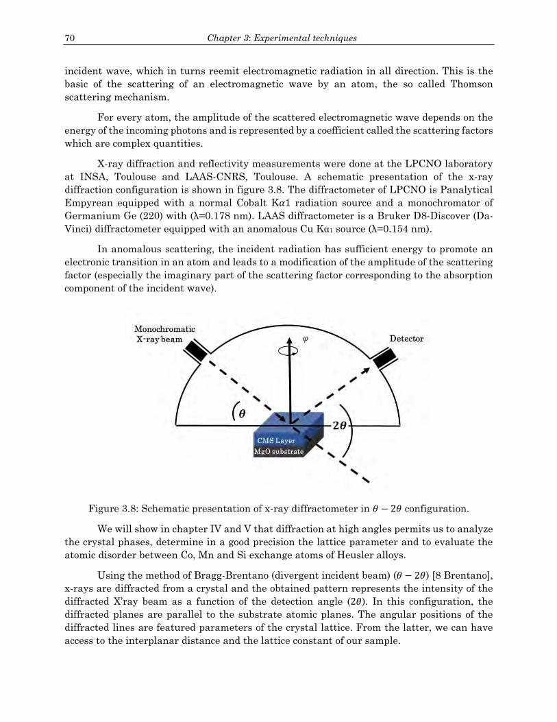
70 Chapter 3: Experimental techniques
incident wave, which in turns reemit electromagnetic radiation in all direction. This is the
basic of the scattering of an electromagnetic wave by an atom, the so called Thomson
scattering mechanism.
For every atom, the amplitude of the scattered electromagnetic wave depends on the
energy of the incoming photons and is represented by a coefficient called the scattering factors
which are complex quantities.
X-ray diffraction and reflectivity measurements were done at the LPCNO laboratory
at INSA, Toulouse and LAAS-CNRS, Toulouse. A schematic presentation of the x-ray
diffraction configuration is shown in figure 3.8. The diffractometer of LPCNO is Panalytical
Empyrean equipped with a normal Cobalt K𝛼1 radiation source and a monochromator of
Germanium Ge (220) with (λ=0.178 nm). LAAS diffractometer is a Bruker D8-Discover (Da-
Vinci) diffractometer equipped with an anomalous Cu Kα1 source (λ=0.154 nm).
In anomalous scattering, the incident radiation has sufficient energy to promote an
electronic transition in an atom and leads to a modification of the amplitude of the scattering
factor (especially the imaginary part of the scattering factor corresponding to the absorption
component of the incident wave).
Figure 3.8: Schematic presentation of x-ray diffractometer in 𝜃 − 2𝜃 configuration.
We will show in chapter IV and V that diffraction at high angles permits us to analyze
the crystal phases, determine in a good precision the lattice parameter and to evaluate the
atomic disorder between Co, Mn and Si exchange atoms of Heusler alloys.
Using the method of Bragg-Brentano (divergent incident beam) (𝜃 − 2𝜃) [8 Brentano],
x-rays are diffracted from a crystal and the obtained pattern represents the intensity of the
diffracted X’ray beam as a function of the detection angle (2𝜃). In this configuration, the
diffracted planes are parallel to the substrate atomic planes. The angular positions of the
diffracted lines are featured parameters of the crystal lattice. From the latter, we can have
access to the interplanar distance and the lattice constant of our sample.
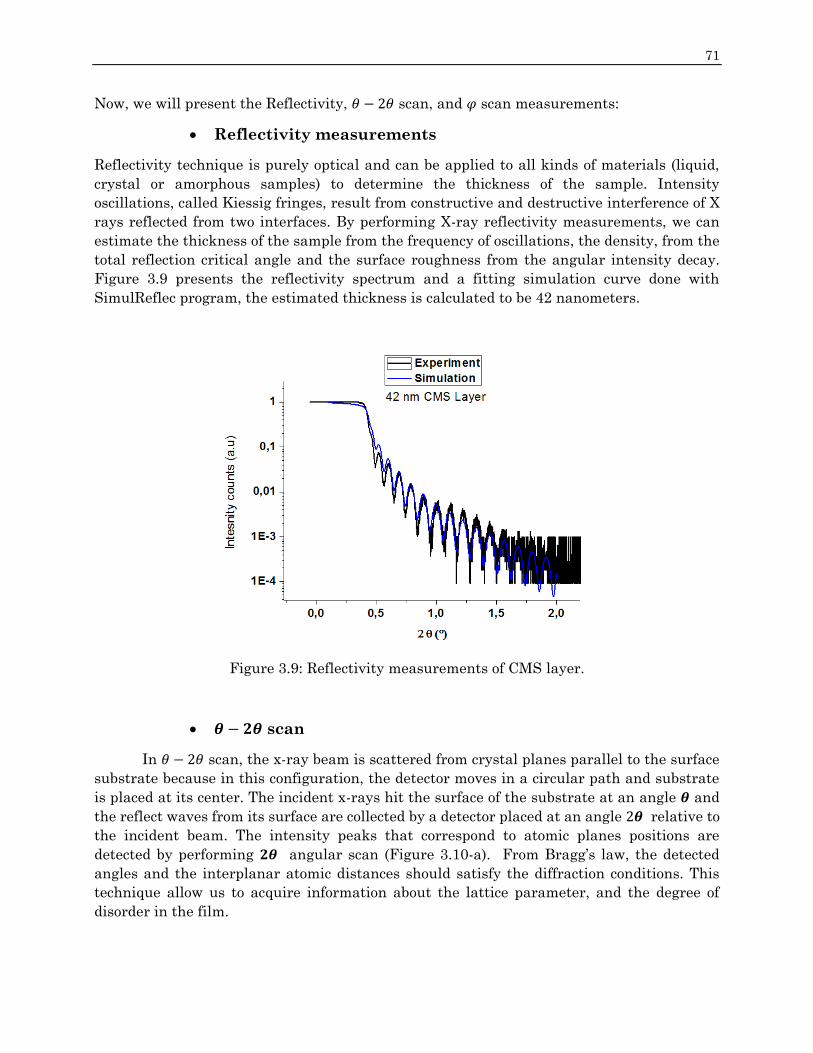
71
Now, we will present the Reflectivity, 𝜃 − 2𝜃 scan, and 𝜑 scan measurements:
Reflectivity measurements
Reflectivity technique is purely optical and can be applied to all kinds of materials (liquid,
crystal or amorphous samples) to determine the thickness of the sample. Intensity
oscillations, called Kiessig fringes, result from constructive and destructive interference of X
rays reflected from two interfaces. By performing X-ray reflectivity measurements, we can
estimate the thickness of the sample from the frequency of oscillations, the density, from the
total reflection critical angle and the surface roughness from the angular intensity decay.
Figure 3.9 presents the reflectivity spectrum and a fitting simulation curve done with
SimulReflec program, the estimated thickness is calculated to be 42 nanometers.
Figure 3.9: Reflectivity measurements of CMS layer.
𝜽 − 𝟐𝜽 scan
In 𝜃 − 2𝜃 scan, the x-ray beam is scattered from crystal planes parallel to the surface
substrate because in this configuration, the detector moves in a circular path and substrate
is placed at its center. The incident x-rays hit the surface of the substrate at an angle 𝜽 and
the reflect waves from its surface are collected by a detector placed at an angle 2𝜽 relative to
the incident beam. The intensity peaks that correspond to atomic planes positions are
detected by performing 𝟐𝜽 angular scan (Figure 3.10-a). From Bragg’s law, the detected
angles and the interplanar atomic distances should satisfy the diffraction conditions. This
technique allow us to acquire information about the lattice parameter, and the degree of
disorder in the film.

72 Chapter 3: Experimental techniques
𝝋 scan
In this configuration, 𝜽 is kept constant (corresponds to a specific diffraction plane) and the
substrate rotates 360° around its surface normal 𝝋 axis. If 𝜽 is fixed at a value equivalent to
the 022 diffracted plane, then for symmetric hkl reflections, we observe 4 peaks in the case of
a cubic lattice. By doing 𝝋 scan for both the MgO substrate and the CMS film on top, we can
confirm the epitaxial relationship and the in-plane 45° orientation. We have performed on our
sample 𝝋 scan for two directions 022 and 111, it shows clearly the 45° orientation of
CMS with respect to the MgO substrate (Figure 3.10-b).
Figure 3.10: a) 𝜽 − 𝟐𝜽 X-ray diffraction scan showing the 002 and 004 peaks of CMS and
002 MgO peak. b) 𝝋 scan of the CMS with respect to the MgO substrate along the 022
direction clearly shows the 45° orientation.
3.3.4 Transmission Electron Microscopy (TEM)
The need in Nano materials sciences to image and examine details down to the atomic
level have resulted in the development of electron microscopes that overcome the resolution
limitation of an optical microscope imposed by the light wavelength. The first transmission
electron microscope was developed by Max Knoll and Ernst Ruska in Germany in 1932. It
consists of a highly energetic electron beam (> 100 keV) accelerated from an electron gun.
This electron beam interacts with a thin sample (< 100 nm thickness) for electron
transparency, before to be visualized on a fluorescent screen or recorded by a charge-coupled
device (CCD) camera. The resulting image gives information about the material morphology
as well as its physical and chemical properties. In this section, we present a general
descriptive of a TEM used in our study. A schematic illustration of a transmission electron
microscope (TEM) is presented in figure 3.11.

73
Figure 3.11: Schematic illustration of a transmission electron microscope.
The TEM column is described as:
An electron gun: to generate the electron beam by either thermoionic gun
or field emission gun (FEG). The thermoionic gun consists of the filament
(cathode), a wehnelt and the anode. The electrons are generated by heating
the metallic filament (Tungsten or LaB6 crystal) and then accelerated
passing them through the wehnelt, which acts as an electromagnetic lens,
and the electron beam converges in a point called “cross-over”, it will be
then accelerated by an accelerator brought at the applied high tension. In
the case of FEG, the electrons are produced by an electric potential applied
between the source and the anode. Electrons are extracted by tunneling
effect. Unlike the thermoionic gun, the electron beam doesn’t pass by a
cross-over, but comes directly from a tungsten filament and accelerated by
a second anode. The two anodes play the role of electrostatic lens (which
permits the convergence of the beam). An image of both thermoionic and
FEG gun is presented in Figure 3.12.

74 Chapter 3: Experimental techniques
Figure 3.12: Schematic illustration of a) the thermoionic Gun principle
and b) the field emission gun FEG [09 Williams and Carter].
Electronic lenses: in the microscope, a converging electron beam is
produced with the help of electromagnetic lenses. Three types of lenses exist
in TEM: condenser, objective and projecting lenses.
1- The condenser lenses: the system of condenser lenses are used to
focus the electron beam on the studied sample either in a parallel or
convergent configuration depending on if we are working in TEM or
scanning transmission electron microscopy (STEM) mode,
respectively. In addition, the use of apertures allows controlling the
electron beam doses to reduce damage in the observed area.
2- Objective lense: it is the most important lens in the column; it is
used to form a magnified image of the specimen. But since
electromagnetic lenses are not perfect, the image contains optical
aberrations that limit the resolution of the microscope such as
spherical aberration, chromatic aberration and astigmatism.
3- Projector lenses: permits to transfer the image formed by the
objective lens and project it on a fluorescent screen and the resulting
light collected by a CCD camera.
In a TEM, the point resolution limit is determined by the lenses performance and the nature
of the electron wave radiation. This is established as the smallest distance between two well-
separated points and is proportional to the product Cs1/4 *3/4, where Cs is the coefficient of
spherical aberration and is the electron wavelength [10 Scherzer]. Thus, the TEM resolution
is limited by the acceleration voltage of the electron beam and the ability to correct the
75
spherical aberration of the objective lens. The most modern TEM microscopes operated at 300
KV and equipped with Cs correctors are able to reach a point-to-point resolution down to 0.5
Å.
A transmission electron microscope has two operational modes: TEM and STEM modes. In
the TEM mode, the image is recorded by using a parallel beam configuration where the
electrons illuminate each point of the specimen at the same time, similar to an optical
microscope. The beam interacts with the specimen and is magnified by the intermediate lens
and then is focused onto an imaging device such as a fluorescent screen or a CCD camera. In
STEM mode, the image is formed by scanning the specimen with a highly focused electron
beam, similar to a scanning electron microscope (SEM).
The local electron-specimen interaction produces several secondary signals that are collected
with different detectors to create a two-dimensional image of the object or analyzed in energy
using a spectrometer to create Electron Energy Loss Spectra (EELS). This feature allows
(S)TEM performing quantitative analysis of the chemical composition of the sample.
Electron-matter interaction:
When an incident electron beam penetrates the sample, electrons undergo elastic or
inelastic scattering. Electrons will be diffused at (milli or micro radian) angles with respect
to the incident electron beam. Inelastic scattering results when the incident electron beam
interacts with the electron cloud of the sample. The energy loss due electron-electron
interaction gives information about the chemical nature, bonding and degree of oxidation in
the studied sample and can be detected using several techniques like Energy Dispersive X-
ray Spectroscopy (EDX), Energy Filtered TEM (EFTEM) or Energy Electron Loss
Spectroscopy (EELS). In elastic scattering process, electrons are scattered without energy
loss. The elastic diffusion results from Coulomb interaction of electrons with the nucleus of
the studied sample. Elastic scattering provides information about the crystalline geometry of
the object.
In this thesis, two TEM modes are used to observe our CMS thin films, the high
resolution TEM (HRTEM) and high angle annular dark field-scanning transmission electron
microscopy (HAADF-STEM) modes. From both techniques we can acquire information
regarding the crystalline structure of the sample depending on the contrast mechanism
involved in the imaging processes. The mentioned modes are discussed in the following two
paragraphs.
3.3.4.1 High Resolution Electron Microscopy (HRTEM):
Starting from the elastic scattering principle, HRTEM images are formed when the
electron wave is phase shifted due a potential distribution within the sample. The electron
wave contains structural characteristics of the sample.
From a mathematical point of view, the image formation by TEM is described as
follows: according to quantum mechanics, a high energetic electron wave that is scattered
from the interaction with the crystalline specimen can be described by the Schrodinger
equation (also known as Dirac equation) with 𝐸, 𝑒 𝑎𝑛𝑑 𝑚 are the energy, charge and mass of
an electron:

76 Chapter 3: Experimental techniques
[−ℏ2
2𝑚∇2 − 𝑒𝑉(𝑟)] 𝜓(𝑟) = 𝐸𝜓(𝑟) (3.2)
By considering the negligible effect of the elastically scattered electrons and absorption
by the thin specimen, the above equation is solved by considering 𝜓(𝑟) as a plane wave:
𝜓(𝑟) = 𝐴(𝑟)𝑒𝑥𝑝𝑖𝜑(𝑟) (3.3)
𝐴(𝑟) and 𝜑(𝑟) being the amplitude and phase shift of the electron plane wave function. This
electron wave propagates through the objective lens that creates a magnified image of the
specimen in its image plane. The final image wave function, image(r), contains information
about both the specimen and the optical system. Mathematically speaking, image(r) will
correspond to the inverse Fourier transform of the product, in the reciprocal space, of the
object electron wave (𝜓𝑜𝑏𝑗(𝐤)𝑇(𝐤)) and the transfer function, T(k), which contains all the
optical transfer (including aberrations and defocus) of the microscope:
𝜓𝑖𝑚𝑎𝑔𝑒(𝐫) = 𝐹𝑇−1𝜓𝑜𝑏𝑗(𝐤)𝑇(𝐤) (3.4)
where FT is the Fourier transform operator.
The recorded TEM image will be the intensity of 𝜓𝑖𝑚𝑎𝑔𝑒(𝑟), I(r) = 𝜓𝑖𝑚𝑎𝑔𝑒(𝑟))2. For an ideal
microscope, the image intensity will correspond to the amplitude of image(r) only. However, a
suitable alteration of the transfer function will allow recovering the phase shift of the image
electron wave. In this way, high-resolution TEM mode allows to get this phase shift, needed
to resolve atomic columns.
The HF3300C 300 KV Cold FEG microscope (I2TEM), developed between Hitachi and
CEMES-CNRS, is used to acquire HRTEM images. It is equipped with a spherical aberration
corrector located below the objective lens which achieve a spatial resolution of 80 pm [11
Snoeck]. An example of a TEM image for CMS sample is presented in figure 3.13.
Figure 3.13: Intermediate-magnification HRTEM image for a cross-sectional CMS
layer grown on MgO substrate.

77
3.3.4.2 Scanning Transmission Electron Microscopy (STEM):
HAADF STEM experiments were done by Dr. César Magen at LMA-INA, Zaragoza-
Spain using FEI TITAN low-base microscope equipped with a spherical probe aberration
corrector which is localized below the condenser lens system and above the objective lens.
In STEM mode, information is collected in a serial acquisition procedure. A small probe
is scanned over the surface of the sample point by point. The image is formed after collecting
signals at each position of the probe. Specific detectors will acquire the electrons scattered at
various angle. There are three types of STEM detectors used: the Bright Field (BF) detector
which permits to captures the unscattered electrons, the Dark Field (DF) detector collects the
diffracted beam of angles between 10 and 40 mrad and the High Annular Dark Field (HAADF)
detector that collects the high angles diffracted beams (angles>40 mrad) (Figure 3.14).
Figure 3.14: various electron detectors in STEM mode [9 William and Carter].
The HAADF detector collects the elastically incoherently scattered electrons resulting
from interaction with the atomic nuclei of the sample [12 Peng]. The signal intensity collected
by the HAADF detector is proportional to the atomic number (Z) of atoms that have interacted
with the electron beam. It means that elements with high atomic number (Z=27 for Co) can
be distinguished from lighter ones (Z=16 for Si). The intensity of the detector is expressed as:
𝐼~𝑚 ∗ 𝑡 ∗ 𝑍𝜂 (3.5)
Where 𝜂 is a constant between √2/3 and 2, m is a scaling constant and t is the sample
thickness. 𝜂 depends on many parameters: for example the convergence of the beam and the
detector, the sample and the orientation of the sample. An example of an HAADF-STEM
image of CMS layer is shown in figure 3.15

78 Chapter 3: Experimental techniques
For more details about STEM technique, the reader is invited to check the following
references [13-16].
Figure 3.15: An HAADF-STEM image of CMS layer where the atomic columns of Co, Mn Si
are clearly shown.
3.3.4.3 Geometric Phase Analysis (GPA):
Geometric Phase Analysis (GPA) is a quantitative method to study the local
deformation field in crystalline materials. This method has been developed by M. Hÿtch and
co-workers [17 Hÿtch, 18 Snoeck, 19 Rocher and Snoeck] and is described briefly as follows:
In a HRTEM/HAADF-STEM image, the different set of fringes can be considered as a
Fourier series (summation of cosine functions). After applying a fast Fourier transform (FFT),
the different sets of fringes are represented as ghkl reflections in the reciprocal space, similar
to a diffraction pattern. A mask is then applied to a reflection in order to isolate the
information corresponding to a single signal and an inverse Fourier transform (FFT-1) is
performed. A complex image is obtained from which we calculate the phase of the chosen
signal (or set of fringes). The recovered phase information (so-called “geometric phase”) is
related to the displacement of the lattice plane by the following expression:
𝜑(𝑔) = −2𝜋. (𝑟) (3.6)
where is the Bragg periodicity and 𝑟 is the position vector in the real space. The lattice
deformation can then be calculated from the gradient of the phase image, in the direction of
the chosen vector. A 2D deformation field can also be calculated using at least two phase
images reconstructed from two non-collinear vectors. A more acquire result is obtained
when GPA method is applied on HAADF-STEM images because of the signal-to-noise ratio
is lower than those images obtained by HRTEM.

79
In Figure 3.16 we describe how we use GPA method for mapping the strain of the in-
plane lattice parameter through the 220 plane: in a HAADF-STEM image obtained close to
the CMS-MgO interface (Figure 3.16 (a)), we calculate the FFT image (Figure 3.16 (b)). Here
we have selected the 220 spot using a cosine mask, as presented by a circle in the FFT. By
solving equation 3.6, we reconstruct an image of the phase, taking as reference the lattice
parameters of MgO, the color variation observed in the CMS layer evidences a lattice
parameter difference between the MgO and CMS in-plane lattice parameters (Figure 3.16
(c)). In figure 3.16 (d) the strain is presented as the 𝜀𝑥𝑥 in-plane deformation that is calculated
from the phase gradient. Here a deformation of -4.6 % was measured in the CMS layer relative
to the MgO substrate lattice parameters.
Figure 3.16: a) HAADF-STEM image of CMS/MgO and its corresponding b) FFT. c)
The phase image and the d) strain mapping.
3.3.4.4 Lorentz Microscopy (LM):
The high spatial resolution of a TEM used to investigate the crystal structure and
chemical composition of thin specimen at nanoscale can be also used to visualize, and
quantitatively study the magnetic configuration of magnetic materials. Electron holography
(EH) and Lorentz Microscopy (LM) are the most popular magnetic imaging TEM techniques
that allow reconstructing the integrated magnetic induction along the electron trajectory and
projected to the image plane, with spatial resolutions ranging from few nanometers (in the
case of LM) to 1 nm (in the case of EH). Both techniques obtain the magnetic information of
a magnetic specimen by retrieving the shift of the electron wave phase after it passes through

80 Chapter 3: Experimental techniques
the sample. However, the way to get this phase shift is different in each case: in EH, the phase
shift is recorded by making a interferometry experiment between two electron waves; in LM,
the phase shift can be obtained by altering the transfer function of the microscope either by
using a contrast aperture to select a particular magnetic deflection direction in the back focal
plane (LM in Foucault mode [20 De Graef]) or by defocusing the image (LM in Fresnel mode).
The later LM mode is a versatile method to get a rapid visualization of magnetic domains via
the observation of magnetic domain walls (DWs). DWs were first observed by Hale in TEM in
1959 [21 Hale] and since then Lorentz microscopy technique gained a lot of success. The
purpose of using this technique is to study the magnetic configuration of magnetic domains
in our CMS thin films, as well as the determination of the exchange constant by measuring
the DW width. In our study we use the LM in Fresnel mode and it is described as follows:
LM in Fresnel mode
From a classical approach, LM is based on the Lorentz force, FL, that experience the
electrons travelling a velocity v when they pass through the electric (E) and magnetic (B)
fields inside and around the ferromagnetic material:
𝐅𝐋 = −𝑒(𝐄 + 𝐯 × 𝐁) (3.7)
In absence of electric fields acting parallel to the image plane, the in-plane component
of the magnetic induction will induce a deflection of the electron trajectory which is
perpendicular to the in-plane magnetic induction direction (B = B(x, y)), according to the
cross product. The electron deflection angle L respect to the incoming electron trajectory can
be calculated as:
𝜃𝐿 =𝑒𝜆
ℎ𝐵⊥𝑡 (3.8)
Where t corresponds to the sample thickness. In presence of these magnetic domains
with different orientations, the electron deflection process creates two bright and dark lines
with excess and lack of electrons respectively imaging the domain wall (DW) separating
neighboring magnetic domains (see figure 3.17). Therefore, in out-of-focus condition, a DW
will produce a brighter and/or a darker contrasts in LM image, and this magnetic contrast
can be inversed by changing the defocus sense. A schematic representation of the magnetic
contrast formation due to DW in LM, in Fresnel mode, is shown in Figure 3.17. Thus LM is a
powerful tool to perform a qualitative description of the magnetic configuration of
ferromagnetic nanostructures by a direct visualization of DWs, and its versatility allows
developing in-situ TEM experiments to follow the evolution of these DWs by the application
of diverse stimuli like magnetic field, electric current, temperature and strain.
For a quantitative analysis, we need to make a more complex treatment that will
permit getting the electron wave phase shift and understand the electron interference process
around a DW that will allow measuring its width.

81
Figure 3.17. Schematic representation illustrating the mechanism of contrast formation by
DWs in Fresnel mode. In top is represented the electron deflection process due to Lorentz
force. In bottom is illustrated the resulting intensity profile traced perpendicular to DWs for
a given defocus position f = z 0. (Adapted from [22 Lloyd])
Quantitative magnetic information by TIE analysis
In LM, the phase shift is obtained by solving the following differential equation in the limit
of small defocus, z:
−2𝜋
𝜆
𝜕𝐼(𝑥,𝑦,Δ𝑧)
𝜕Δ𝑧|Δ𝑧→0
= ∇ ∙ [𝐼(𝑥, 𝑦, 0)∇φ(x, y)] (3.9)
Equation 3.9 is the so-called transport of intensity equation (TIE) [23 Beleggia], and show
how the phase shift gradient is proportional to the derivate of the intensity with respect to
the defocus. This equation proposed by Van Dyck et. al. [24, 25 Van Dyck] arises by calculating
the intensity of the image electron wave, ima(r), considering a small alteration of the transfer
function of the microscope due to a small defocus. Equation 3.9 can be solved by means of a
focal series of Lorentz images, where images are recorded in-focus [I(x, y, 0)], under-focus [I(x,
y, -z)] and over-focus [I(x, y, z)], conditions are used to calculate (x, y) after rewriting the
equation 3.9:
∇𝜑(𝑥, 𝑦) = −𝜋
𝜆Δ𝑧∇−2∇ [
1
𝐼(𝑥,𝑦,0)∇∇−2[𝐼(𝑥, 𝑦, Δ𝑧) − 𝐼(𝑥, 𝑦, −Δ𝑧)]] (3.10)
where -2 is the two-dimensional inverse Laplacian operator. While Lorentz force describes
the ‘classical’ movement of the electrons inside electromagnetic fields, in a quantum

82 Chapter 3: Experimental techniques
mechanics approach the Aharanov-Bohm effect describes how the phase of the electron wave
is shifted by the influence of these electromagnetic potentials:
𝜑(𝑥, 𝑦) = 𝐶𝐸 ∫𝑉(𝑥, 𝑦, 𝑧)𝑑𝑧 −𝑒
ℏ∫𝐴𝑧(𝑥, 𝑦, 𝑧)𝑑𝑧 (3.11)
where CE is a interaction constant that only depends on the acceleration voltage of the
microscope, V is typically the electrostatic potential of the specimen and Az is the z-component
of the magnetic potential. If we assume that the specimen is chemically homogeneous and its
thickness is constant, the phase shift gradient calculated by TIE method can be associated
with the in-plane magnetic induction as:
∇𝜑(𝑥, 𝑦) = −𝑒
ℏ[𝐧𝑧 × 𝑡𝐁(𝑥, 𝑦)] (3.12)
where nz is the z-component of the normal vector which is perpendicular to the sample plane.
Equation 3.12 can be also expressed in term of B(x, y) as:
𝐁(𝑥, 𝑦) = (𝐵𝑥 , 𝐵𝑦) =ℏ𝑡
𝑒(−
𝜕𝜑
𝜕𝑦,𝜕𝜑
𝜕𝑥) (3.13)
Thus the above vector expression will allow the reconstruction of vector maps of the in-plane
magnetic induction, providing us a quantitative description of local magnetization
orientation.
Measurement of DW width
By LM in Fresnel mode we can measure the width of DWs by taking advantage of the
linear behavior between the width of magnetic contrast (Wc) and the defocus distance, where
the magnetic contrast width increases with the increasing of the absolute value of the defocus
distance. As commented previously, the different magnetization orientations of neighboring
magnetic domains can produce either a bright contrast due to the accumulation of electrons
or a dark contrast due to the deficient of them in the DW position. Another way to see this
phenomenon is to think that a bright contrast is produced because of two images of both
domains are moved toward the center of the DW, overlapping them, causing a convergent
image interference, while a dark contrast is produced because of the two image are moved
outside the center of the DW, separating them, causing a divergent image interference. As we
see in Figure 3.18, while a divergent image interference induces a single valley, or inverted
peak, in the intensity profile, a convergent image interference produces a fringe pattern due
to the superposition of two electron waves that converge in the middle of the DW. Both
contrast can be used to measure DW widths, but the bright one is more tricky because is more
difficult to determine the width of the fringe pattern.
For Bloch walls, the domain wall width can be measured by using a simple analytical
expression for convergent- and divergent-wall width versus defocus distance [26 Wade, 27
Volkov]:
𝑊𝐶 = 𝑊𝐷𝑊 + 2𝜃𝐿∆𝑧 (3.14)

83
𝑊𝐷𝑊 corresponds to the DW. Thus, 𝑊𝐷𝑊 can be calculated from the above equation by a
straightforward extrapolation to z = 0 of a linear regression of the function 𝑊𝐶(∆𝑧). In
addition, the linear regression slope gives us information about the deflection angle 𝜃𝐿,
parameter that can be also estimated from equation 3.8 if we know the magnetic induction of
the specimen and the sample thickness around the DW. The main drawback of equation 3.8
is that we have to know previously the effective thickness, parameter that is not easy to
obtain. Fortunately, there is a way to estimate the product Bt by measuring the fringe
spacing created in the convergent image (Figure 3.18-d) for the bright magnetic contrast at
high defocus values. If we assume that the magnetic field away from the DW is uniform so:
𝐵⊥𝑡 =ℎ
𝑒
1
2𝑠 (3.15)
Where ‘s’ is the spacing of the fringes for a bright contrast. From equation 3.8 and 3.15 we
can easily deduce that the slope of equation 3.14 is directly related with 1/s as:
2𝜃𝐿 =𝜆
𝑠 (3.16)
Thus, equation 3.16 can be used as an accuracy parameter of linear regression to
determine the DW width of Bloch walls. In the case of Néel wall, the DW width determination
is not straightforward, because its magnetic structure is more complex and we do not know if
the DW width measured by Lorentz Microscopy corresponds to either the width of the core or
tail Néel wall.
An example of the CMS layer taken at different defocus values is presented in figure
3.18. In chapter 4, we will show the results of DW observed by LM technique.
Figure 3.18: observation of domains walls in a) over-focus ∆𝑧> 0 and c) under-focus
( ∆𝑧< 0). Image b) corresponds to the in-focus ( ∆𝑧= 0) observation where no magnetic
domains are observed. Figure d) shows the fringe spacing of the red box in a)
84 Chapter 3: Experimental techniques
3.4 Magnetic characterization techniques
Ferromagnetic resonance (FMR), Longitudinal Magneto-Optical Kerr Microscope
(LMOKE) and Physical Property Measurement System (PPMS) are the techniques used in
this thesis work to study the static and dynamic magnetic properties of CMS films. The
mentioned techniques will be detailed as follows:
3.4.1 Physical Property Measurement System (PPMS)
Magnetic moment measurements of the CMS films have been performed at the
“Laboratoire de Physique et Chimie des Nano-Objets” (LPCNO), Toulouse. These
measurements have been performed with a PPMS-VSM device from Quantum Design. This
magnetometry measurement is based on the variation of magnetic flux induced in two pickup
coils by a vibrating sample. One of the main advantages of this device is the possibility to
apply large fields up to 9 T and to perform measurements down to 2 K. However, our
experiments have been performed in magnetic fields up to 1T at room temperature.
3.4.2 Magneto-Optical Kerr Effect (MOKE)
The interaction between light and a magnetic medium is known for more than a century since
the discovery of the Faraday Effect in 1875 and the Kerr effect in 1877. The Faraday Effect
corresponds to the rotation of the polarization axis of a linearly polarized electromagnetic
wave travelling through a dielectric and simultaneously submitted to an external magnetic
field parallel to the propagation direction. This effect is due to the difference of propagation
velocity for the right and left handed waves composing the initial wave. In a simple
approximation, the rotating electric field of the circularly polarized wave induces a circular
electric polarization in the material, which in turn creates a magnetic field. Depending upon
the polarization (right or left), the additional magnetic field oppose or add up to the
magnetization (or magnetic field) and leads to a decrease or increase in the velocity. It is
important to note that the rotation of the polarization is reversed if the magnetic field is
reversed.
The Kerr effect is the equivalent of the Faraday Effect but for the reflected component of the
incident wave. In the case of a magnetic sample, it is the magnetization of the sample which
acts as the effective magnetic field. In this case we talk about the Magneto-Optical Kerr Effect
(MOKE). In reflection, there is also a second effect that induces a rotation of the polarization
and some ellipticity (Figure 3.19-b). It is called the Voigt effect and it is proportional to the
square of the normalized component of the magnetization. However this effect is generally
lower than the Kerr effect and is often neglected.

85
Figure 3.19: Schematic illustration of a polarized wave before a) and after b) the reflection.
Therefore, in a MOKE experiment, the polarization of a linearly polarized light reflected at
the surface of a magnetic material will depend on the direction of the magnetization with
respect to the propagating wave vector. Three experimental configurations are possible
depending on the orientation of the magnetization with respect to the plane of incidence (see
Figure 3.20). In the polar configuration (PMOKE) the magnetization is perpendicular to the
plane of the layer and in the incident plane of the light. In the longitudinal configuration
(LMOKE) the magnetization lies in plane of the layer and in the incident plane (Fig 3.20-b).
In the transverse configuration (TMOKE or Quadratic MOKE QMOKE) the magnetization
lies in the plane of the layer and is perpendicular to the incident plane (Fig 3.20-c).
Figure 3.20: a) Polar, b) Longitudinal and c) Transverse configurations of MOKE.
In this work, the magnetization of the CMS films has been studied in the LMOKE
configuration. The set-up is located on the ONERA campus. The experiment is schematized
in Figure 3.21. It is composed of a Laser source He-Ne with a 5 mW power. Before the sample,
a Glan-Thomson polarizer (P) allows to linearly polarize the light. A magnetic field is applied
parallel to the plane of the sample by two Helmotz coils. The magnetic field can reach 450 Oe.
The reflected wave is analyzed with an analyzer composed of a rotary retardation plate, set

86 Chapter 3: Experimental techniques
to get a rotation of the polarization at 45° with respect to the polarization at the output of (P),
and a Wollaston bi-prism. The latter allows to separate the reflected wave into two equal
components. Finally each component will be measured by two PIN photo-diodes and their
difference is recorded as a function of the applied field. Prior to the experiment, the intensity
on each diode is set to be equal in absence of external field. Then the field is applied back and
forth in a sequence zero->+saturation-> - saturation-> +saturation.
An example of a LMOKE measurement of the hysteresis curve on our sample is presented in
Figure 3.22.
Figure 3.21: schematic illustration of MOKE experimental set-up.
Figure 3.22: An example of Hysterises loop for LMOKE measurements.
3.4.3 Ferromagnetic Resonance (FMR)
Ferromagnetic resonance (FMR) spectroscopy is one of the techniques used to probe
electrons spin magnetic moments and study magnetic properties and spin dynamics of

87
ferromagnetic materials. FMR was first discovered in 1911 by Arkadyév after he observed the
absorption of Ultra High Frequency radiation in ferromagnetic materials. In 1923, the results
of Arkad’yev were explained by Dorfman as an optical transition due to Zeeman splitting from
which it provides a way to study ferromagnetic materials. As explained in chapter 2, FMR is
based on the absorption of microwave field of a few GHz by a ferromagnetic material. This
section provides an overview about the experimental setup used to extract the magnetic
parameters in this work.
3.4.3.1 FMR Experimental set-up
During this PhD work, we have developed a FMR measurement set-up at the CEMES
Lab. We used the well-known modulation technique, first because of the easiness to set, as it
avoids complicated calibration procedure like in vectorial measurements, and also to get a
good signal to noise ratio.
Our experiment is depicted and schematically illustrated in Figure 3.23. The principle
of the measurement is the following. A microwave signal of given frequency is injected in a
microstrip line above which the CMS sample is placed. In this work, the injected microwave
power in the stripline is about -15 dBm. Such amplitudes of the microwave signal allows to
stay in the linear regime of excitation of the spin dynamics. The microstrip line is placed in
an electromagnet allowing for a static magnetic field to be applied. Additionally Helmholtz
coils are fed with a low frequency current which allows modulating the static field. In this
experiment the static magnetic field is swept and the frequency of the microwave signal is
constant. At the resonance field, the magnetic sample absorbs some energy from the
microwave field (called the pumping field). The decrease of the microwave amplitude is
measured in transmission via a schottky diode and a lock in amplifier. All instruments are
piloted via a homemade LabVIEW interface program.
The maximum static magnetic field that can be applied is equal to 0.7 T for a field
applied in the plane of the layer and 1.5 T for a perpendicular applied field. This is achieved
by changing the poles of the electromagnet. Also, our set-up allows for a rotation of the
electromagnet from 0 to 180°.This allows to study the angle dependence of the FMR signal in
plane. The low frequency generator feeds a Kepco current source which is connected to the
Helmoltz coils. The frequency of the voltage signal sent by the generator to the Kepco and
then the frequency of magnetic modulation is set to 73 Hz. The amplitude of the modulation
field is of 2 Oe. The same voltage signal that feeds the Kepco is injected to the reference input
of the lock-in for the demodulation measurement.
The microstrip line has been fabricated at ONERA-Toulouse clean room facility from
a 350 µm thick Alumina wafer with a dielectric constant ≈ 10. The dielectric is fully covered
by gold on one side in order to connect to the ground plane of the sample holder made of brass.
On the other side of the dielectric, a gold line of 400 µm width has been realized by UV
lithography. The width has been chosen in order to be as close as possible to 50 ohms and also
to facilitate the connection with the central core of SMA connectors. As can be shown from
the reflection and transmission measurement in Figure 3.24, the line is clearly not 50 ohms

88 Chapter 3: Experimental techniques
adapted within all the frequency range. The periodic modulation of the transmitted S21 or
reflected S11 signal, measured with an Anritsu MS4642A vector network analyzer, comes
from the impedance mismatch between the line and the connectors. The S11 and S21
parameters corresponds to the coefficient of reflection and transmission, respectively of the
incident microwave voltage signal. The most probable reason is a bad value of the dielectric
constant considered to design the line. Due to the difficulty to get access to lithography
facilities, all measurements presented in this work have been performed with this microstrip
line.
Figure 3.23: depicted presentation and schematic illustration of the
FMR set-up.
0 5 10 15 20
-40
-30
-20
-10
0
dB
GHz
S11
S12
Figure 3.24: Reflection “S11” and transmission “S12” measurements of the
transmission line.

89
Now let us study the response of magnetic material to electromagnetic radiation at a
fixed frequency 𝜔0. As explained in chapter 2 (section 2.3.1), the magnetic susceptibility is
complex and equals to 𝜒′ + 𝑖 𝜒′′ . It is the imaginary part of the susceptibility that corresponds
to the energy losses and to microwave absorption. However, modulating the value of the static
field, the absorption is also modulated. Experimentally it corresponds to the measurements
of the derivative of 𝜒′′(𝜔)
Let’s consider the pumping field to be of the form ℎ(𝑡, 𝜔) = ℎ0𝑒𝑖𝜔𝑡. Following 𝑚(𝑡, 𝜔) =
𝑚(𝑡, 𝜔)𝑒𝑖(𝜔𝑡+𝛿), the dynamic component of the magnetization is of the form
𝑚(𝑡, 𝜔) = (𝜒′ + 𝑖𝜒")ℎ0𝑒𝑖𝜔𝑡. The variation of the free energy of the system can be written as
dF=−μ0h.dm. Then the average power dissipated by the magnetic system can be written as:
𝑃𝑎𝑏𝑠𝑜𝑟𝑏𝑒𝑑𝑡𝑜𝑡 = lim
𝑇→∞
µ0
𝑇∫ 𝑅𝑒(ℎ). 𝑅𝑒 (
𝑑𝑚
𝑑𝑡) 𝑑𝑡 =
1
2μ0𝜔𝜒
′′(𝜔)𝑇
0ℎ02 (3.17)
Experimentally, we measure the variation of the transmitted voltage in the microstrip line
due to the absorbed power in the magnetic film. The variation of voltage is due to the inductive
coupling between the microstrip and the magnetic sample. Figure 3.25 gives a very simplified
vision of the transmitted signal. We see that due to modulation of the static field at
frequency, 𝑓𝑚𝑜𝑑𝑢𝑙𝑎𝑡𝑖𝑜𝑛, the amplitude of transmitted amplitude varies also as 𝑓𝑚𝑜𝑑𝑢𝑙𝑎𝑡𝑖𝑜𝑛 and
is proportional to 𝑑𝜒′′/𝑑ℎ. Using a Shcottky diode allows to recover the envelop function (red
line in Fig. 3.26) as the output voltage is given by √𝑣(𝑡)2. This low frequency voltage is then
injected at the input of the lock-in.
Therefore, the signal measured with the lock-in is proportional to the derivative of the
susceptibility (Figure 3.26). This technique has the major advantage of increasing the signal
to noise ratio and it is easy to set-up as it avoids complicated calibration process that must be
performed for example with Vector Network Analyzer.
Figure 3.25: Transmitted signal with the red envelope curve.
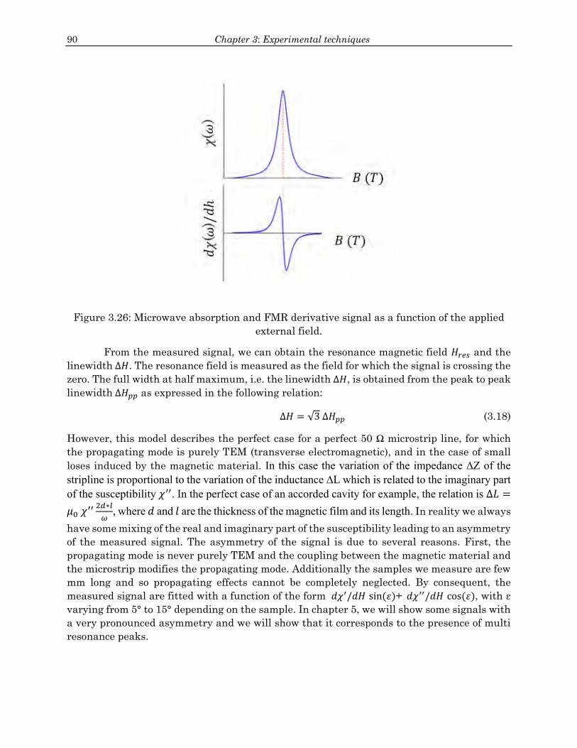
90 Chapter 3: Experimental techniques
Figure 3.26: Microwave absorption and FMR derivative signal as a function of the applied
external field.
From the measured signal, we can obtain the resonance magnetic field 𝐻𝑟𝑒𝑠 and the
linewidth ∆𝐻. The resonance field is measured as the field for which the signal is crossing the
zero. The full width at half maximum, i.e. the linewidth ∆𝐻, is obtained from the peak to peak
linewidth ∆𝐻𝑝𝑝 as expressed in the following relation:
∆𝐻 = √3 ∆𝐻𝑝𝑝 (3.18)
However, this model describes the perfect case for a perfect 50 Ω microstrip line, for which
the propagating mode is purely TEM (transverse electromagnetic), and in the case of small
loses induced by the magnetic material. In this case the variation of the impedance ∆Z of the stripline is proportional to the variation of the inductance ∆L which is related to the imaginary part of the susceptibility 𝜒′′. In the perfect case of an accorded cavity for example, the relation is ∆𝐿 =𝜇0 𝜒
′′ 2𝑑∗𝑙
𝜔, where 𝑑 and 𝑙 are the thickness of the magnetic film and its length. In reality we always
have some mixing of the real and imaginary part of the susceptibility leading to an asymmetry
of the measured signal. The asymmetry of the signal is due to several reasons. First, the
propagating mode is never purely TEM and the coupling between the magnetic material and
the microstrip modifies the propagating mode. Additionally the samples we measure are few
mm long and so propagating effects cannot be completely neglected. By consequent, the
measured signal are fitted with a function of the form 𝑑𝜒′/𝑑𝐻 sin(𝜀)+ 𝑑𝜒′′/𝑑𝐻 cos(𝜀), with ε
varying from 5° to 15° depending on the sample. In chapter 5, we will show some signals with
a very pronounced asymmetry and we will show that it corresponds to the presence of multi
resonance peaks.

91
3.5 Ion irradiation/implantation technique
Ion implantation/irradiation consists of accelerating energetic ions into a material with a
fixed energy. The ions which are penetrating can induce some displacement within the sample
in the irradiation regime or to be localized/implanted inside the material in the implantation
regime. The two regimes depends on the kinetic energy of the incoming atoms. Ionic
bombardment was first introduced by Shockley in 1954 at Bell laboratories but later in 1970’s
the ionic implantation technique was developed to introduce impurities in the studied
systems. As mentioned in chapter 1, this technique is highly desired to modify the structural
electronic and magnetic properties for electronic systems and industrial applications. The
main application of this technique is the doping of semiconductor materials for the fabrication
of integrated electronic devices. Implantation/irradiation can be done with almost all the
elements such as Ga, He, Cr, Si and many others.
During this thesis, the ion irradiation of Heusler alloys is carried out at room temperature
in CEMES laboratory using an ion implanter VARIAN 200-A2F. This ion implanter (Figure
3.27) consists of:
Ion source: which converts the electrically neutral atoms (Arsine,
Phosphorus or helium…) from the gas phase into an ion plasma and
impurities. These ions are extracted with voltage of 25 kV.
Mass spectrometer: consists of a magnetic sector which bends the ion beam
through a right angle, spatially separate the different masses present in the
beam and select desired ions species passing through a selection aperture
before reaching the accelerator.
Accelerator: It will increase the ion energy up to 200 KeV to the ions to be
implanted.
Focusing and Scanning system: a quadrupole lens and deflection plates in
x and y directions to focus and scan the ion beam on the selected sample to
produce uniform implantation/ irradiation with a desired fluence.
Figure 3.27: schematic illustration of ion implanter.

92 Chapter 3: Experimental techniques
3.5.1 Ion-Solid interaction
When an ion beam bombards a solid material, several mechanisms will take place to
slow down the accelerated ions and dissipate their energy. These mechanisms are divided into
1) nuclear energy losses which occur as a result of elastic collision where the energy is
transferred from the kinetic incident ion to the target atoms, and 2) electronic energy losses
which occur as a result of inelastic scattering where the electrons of the ions interact with the
electrons of the target atoms [28 Giannuzzi]. The interaction mechanism is traditionally
divided in a nuclear and an electronic stopping power. The ion energy loss is characterized by
the sum of both terms. The contribution of each effect varied along the trajectory of the ions.
Finally, both mechanisms define the stopping range of an ion energy loss in a path length and
the final ion concentration distribution (figure 3.28). The stopping power range is expressed
as follows:
𝑆 = (𝑑𝐸
𝑑𝑥)𝑛𝑢𝑐𝑙𝑒𝑎𝑟
+ (𝑑𝐸
𝑑𝑥)𝑒𝑙𝑒𝑐𝑡𝑟𝑜𝑛𝑖𝑐
(3.19)
Nuclear energy losses are dominant to explain ion-solid interaction for low energy
accelerated ions with high atomic number, but electronic energy losses becomes important for
high energy accelerated ions with low atomic numbers. In nuclear energy loss process, the
accelerated ions will transfer energy to the target atoms which can be displaced from their
initial position (lattice sites) if the energy is high enough. These recoil atoms can also induce
the displacement of the lattice sites as far as their energy is larger than a threshold value.
This is known as the collision cascade. This leads to the movement of the ion to an interstitial
site by leaving a vacancy in the target lattice site. The vacancy-interstitial pair is called the
Frenkel pair or Frenkel defect. The displaced atoms can undergo further collisions in their
way through the material which leads to other types of defects like dislocations characterized
by local lattice heating of the target material. Electronic losses have less lattice disorder
impact on the target lattice than the nuclear energy losses due to the small energy transfer
collision [29 Gaier].
Figure 3.28: stopping range power as a function of ion velocity.

93
Chapter 3 References:
[1] D. K. Fork, D. B. Fenner, G. a. N. Connell, J. M. Phillips, and T. H. Geballe, “Epitaxial
yttria‐stabilized zirconia on hydrogen‐terminated Si by pulsed laser deposition,” Appl.
Phys. Lett., vol. 57, no. 11, pp. 1137–1139, Sep. 1990.
[2] A. Inam, C. T. Rogers, R. Ramesh, K. Remschnig, L. Farrow, D. Hart, T. Venkatesan, and
B. Wilkens, “a‐axis oriented epitaxial YBa2Cu3O7−x‐PrBa2Cu3O7−y heterostructures,”
Appl. Phys. Lett., vol. 57, no. 23, pp. 2484–2486, Dec. 1990.
[3] D. M. Hwang, T. Venkatesan, C. C. Chang, L. Nazar, X. D. Wu, A. Inam, and M. S. Hegde,
“Microstructure of insitu epitaxially grown superconducting Y‐Ba‐Cu‐O thin films,” Appl.
Phys. Lett., vol. 54, no. 17, pp. 1702–1704, Apr. 1989.
[4] P. Willmott, “Deposition of complex multielemental thin films,” Prog. Surf. Sci., vol. 76,
no. 6–8, pp. 163–217, Oct. 2004.
[5] Cho, A. Y.; J. R. Arthur, Jr. ‘Molecular beam epitaxy. Prog. Solid State Chem., 10: 157–
192. (1975).
[6] P. Turban, S. Andrieu, B. Kierren, E. Snoeck, C. Teodorescu, and A. Traverse, “Growth
and characterization of single crystalline NiMnSb thin films and epitaxial
NiMnSb/MgO/NiMnSb(001) trilayers,” Phys. Rev. B, vol. 65, no. 13, Mar. 2002.
[7] G. Ortiz Hernandez, “Elaboration et étude des propriétés physiques de couches minces
monocristallines d’alliage de Heusler à faible amortissement magnétique pour
composants hyperfréquences,” Université de Toulouse, Université Toulouse III-Paul
Sabatier, 2013.
[8] J. Brentano, “Focussing method of crystal powder analysis by X-rays,” Proc. Phys. Soc.
Lond., vol. 37, no. 1, p. 184, 1924.
[9] D. B. Williams and C. B. Carter, Transmission electron microscopy: a textbook for
materials science, 2nd ed. New York: Springer, 2008.
[10] O. Scherzer, “The Theoretical Resolution Limit of the Electron Microscope,” J. Appl.
Phys., vol. 20, no. 1, pp. 20–29, Jan. 1949.
[11] E. Snoeck, F. Houdellier, Y. Taniguch, A. Masseboeuf, C. Gatel, J. Nicolai, and M.
Hytch, “Off-Axial Aberration Correction using a B-COR for Lorentz and HREM Modes,”
Microsc. Microanal., vol. 20, no. S3, pp. 932–933, Aug. 2014.
[12] Y. Peng, P. D. Nellist, and S. J. Pennycook, “HAADF-STEM imaging with sub-
angstrom probes: a full Bloch wave analysis,” J. Electron Microsc. (Tokyo), vol. 53, no. 3,
pp. 257–266, 2004.
[13] H. Rose and C. F. Kisielowski, “On the Reciprocity of TEM and STEM,” Microsc.
Microanal., vol. 11, no. S02, Aug. 2005.
[14] D. W. M.I. Den Hertog, “Characterization of silicon nanowires by transmission
electron microscopy,” Acs Nano, vol. 3, no. 10, pp. 3015–3022, 2009.
[15] S. Bals, R. Kilaas, and C. Kisielowski, “Nonlinear imaging using annular dark field
TEM,” Ultramicroscopy, vol. 104, no. 3–4, pp. 281–289, Oct. 2005.
[16] S. Bals, B. Kabius, M. Haider, V. Radmilovic, and C. Kisielowski, “Annular dark field
imaging in a TEM,” Solid State Commun., vol. 130, no. 10, pp. 675–680, Jun. 2004.
[17] M. J. Hÿtch, E. Snoeck, and R. Kilaas, “Quantitative measurement of displacement
and strain fields from HREM micrographs,” Ultramicroscopy, vol. 74, no. 3, pp. 131–146,
août 1998.

94 Chapter 3: Experimental techniques
[18] E. Snoeck, B. Warot, H. Ardhuin, A. Rocher, M. J. Casanove, R. Kilaas, and M. J.
Hÿtch, “Quantitative analysis of strain field in thin films from HRTEM micrographs,”
Thin Solid Films, vol. 319, no. 1–2, pp. 157–162, avril 1998.
[19] A. Rocher and E. Snoeck, “Misfit dislocations in (001) semiconductor heterostructures
grown by epitaxy,” Mater. Sci. Eng. B, vol. 67, no. 1–2, pp. 62–69, décembre 1999.
[20] “De Graef M 2001 Lorentz microscopy: Theoretical basis and image simulations
Magnetic Imaging and Its Applications to Materials. Experimental Methods in the
Physical Sciences vol 36 pp 27–67.”
[21] Hale M E, Fuller H W and Rubinstein H 1959 Magnetic Domain Observations by
Electron Microscopy J. Appl. Phys. 30 789. Springer Science & Business Media, 1998.
[22] S. J. Lloyd, N. D. Mathur, J. C. Loudon, and P. A. Midgley, “Magnetic domain-wall
width in La 0.7 Ca 0.3 MnO 3 thin films measured using Fresnel imaging,” Phys. Rev. B,
vol. 64, no. 17, Oct. 2001.
[23] M. Beleggia, M. A. Schofield, V. V. Volkov, and Y. Zhu, “On the transport of intensity
technique for phase retrieval,” Ultramicroscopy, vol. 102, no. 1, pp. 37–49, Dec. 2004.
[24] D. V. Dyck, “High-speed computation techniques for the simulation of high resolution
electron micrographs,” J. Microsc., vol. 132, no. 1, pp. 31–42, Oct. 1983.
[25] Van Dyck D and Op de Beek M 1993 A new approach to object wavefunction
reconstruction in electron microscopy Optik (Stuttg). 3 103–7.”
[26] R. H. Wade, “The Determination of Domain Wall Thickness in Ferromagnetic Films
by Electron Microscopy,” Proc. Phys. Soc., vol. 79, no. 6, p. 1237, 1962.
[27] V. V. Volkov and Y. Zhu, “Magnetic structure and microstructure of die-upset hard
magnets RE13.75Fe80.25B6 (RE=Nd, Pr): A possible origin of high coercivity,” J. Appl.
Phys., vol. 85, no. 6, pp. 3254–3263, Mar. 1999.
[28] L. A. Giannuzzi, B. I. Prenitzer, and B. W. Kempshall, “Ion-solid interactions,” in
Introduction to focused ion beams, Springer, 2005, pp. 13–52.
[29] O. Gaier, “A study of exchange interaction, magnetic anisotropies, and ion beam
induced effects in thin films of Co2-based Heusler compounds,” Ph. D. dissertation,
Technical University of Kaiserslautern, 2009.

95
Chapter 4: Structural and
magnetic properties of as
deposited CMS samples
As explained in the introduction of this thesis, the particular magnetic features of the
Co2MnSi, such as the half metallicity and low gilbert damping coefficient, are obtained in the
most ordered crystal phase L21 even if half metallicity is also predicted for the B2 order.
Therefore, high crystalline quality of the CMS films is required.
In this work, our goal is to study how the structural order and magnetic properties in
the CMS are correlated. Ion irradiation is used in order to modify and control the structure
of the material and follow the evolution of the different magnetic parameters, especially in
the dynamic range. We will show the results obtained on three series of CMS samples which,
despite similar deposition conditions, show different structural and magnetic properties,
either as deposited or under ion irradiation. Each series of samples corresponds to a thin film
of CMS which is cut into few pieces, one is kept as the “reference” sample and the others
pieces are irradiated at different fluences in order to follow the evolution of the structural and
magnetic properties with irradiation and then with atomic disorder.
The three series of samples are denoted samples N°1, 2 and 3, each showing different
interest and giving different insight into the correlation between the structure and magnetic
properties of the CMS:
- Series N°1: the reference sample shows clearly two distinct crystal orders with
distinct magnetic properties. Also the damping coefficient shows an anisotropic
behavior for the reference sample (i.e. similar behavior in the 4 easy and hard
axes). A complete magnetic and structural characterization of the four samples of
this series has been performed.
- Series N°2: the reference sample shows a single crystal order with a lower
magnetization value than observed for the reference sample of series N°1, but with
a much stronger cubic and uniaxial anisotropy fields. The damping is also found to
be anisotropic. Unfortunately only partial structural characterization could be
performed on this series due to the small size of the samples.
- Series N° 3: it also shows two crystal orders for the reference sample with magnetic
properties similar to those of the reference sample of series N°1. However, in
opposite to series N°1, one of the crystal order is largely minority in the reference
sample as it is barely visible in magnetic measurements. Furthermore, the
reference sample shows an isotropic behavior of the damping coefficient. Here also
only partial structural characterization could be performed on this series.

96 Chapter 4: Structural and magnetic properties of “as deposited” CMS Heusler alloys
In this chapter we will focus on the structural and magnetic properties of the reference
samples of each series. Those ones will be referred in this chapter as sample N°1, 2 and 3. We
first present the methodology to determine the deposition conditions. Then a detailed study
of the structural properties of the reference sample of series N°1 is presented and comments
on the structural properties of samples N°2 and N°3 are given based on partial X-ray
diffraction studies. The last part of this chapter will be devoted to the determination of the
magnetic parameters of the 3 different samples.
4.1 Structural properties of CMS samples
In this section, we first present the deposition conditions of the CMS films studied in this
work. Then we investigate its crystallographic properties by X-ray diffraction and HAADF-
STEM imaging. X-ray allows getting access to the lattice parameters of the structure, degree
of disorder. HAADF-STEM will be used for investigation of local chemical ordering of the alloy
and the lattice mismatch with respect to the MgO substrate.
4.1.1 Determination of deposition conditions
We fabricated our samples with a sputtering chamber located at the CEMES
laboratory (see chapter 3 for details). We present in this chapter the structural and magnetic
properties of 3 samples deposited at 600° C and annealed at 700°C for one hour.
Our first task was to optimize the deposition conditions to fabricate high crystal order
CMS films, i.e. the deposition and annealing temperature. We start from the PhD work of G.
Ortiz [1 Ortiz] who developed the process of CMS thin films deposition with the same
sputtering chamber used in this work. In our study we have also optimized the deposition
conditions of CMS. Our methodology has been the following. First, we studied the effect of the
deposition temperature. We start with a deposition temperature ranging from 400° and up to
700° with 50° step. Each film is annealed at 700° for 1 hour. In order to verify the “quality” of
the film, we performed in-situ RHEED diffraction and ex-situ FMR measurements.
The interest in these two methods is simple. First RHEED gives information about the
surface obtained with a 2 nm penetration depth of 20 kV accelerated electrons. RHEED is
performed at each step of the process and allows for a direct observation of the nature of the
growth (2D, 3D). An example of RHEED images is presented in Figure 4.1 for different
deposition temperatures.
Figure 4.1: RHEED patterns of CMS at different deposition temperatures.
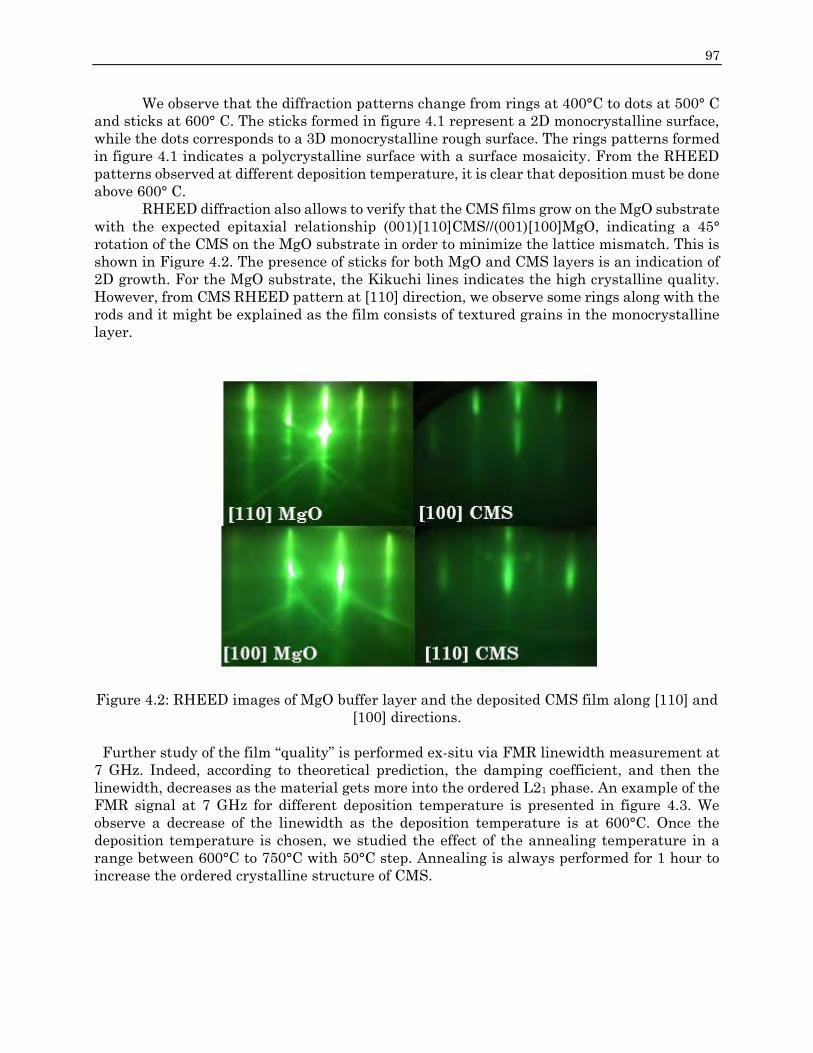
97
We observe that the diffraction patterns change from rings at 400°C to dots at 500° C
and sticks at 600° C. The sticks formed in figure 4.1 represent a 2D monocrystalline surface,
while the dots corresponds to a 3D monocrystalline rough surface. The rings patterns formed
in figure 4.1 indicates a polycrystalline surface with a surface mosaicity. From the RHEED
patterns observed at different deposition temperature, it is clear that deposition must be done
above 600° C.
RHEED diffraction also allows to verify that the CMS films grow on the MgO substrate
with the expected epitaxial relationship (001)[110]CMS//(001)[100]MgO, indicating a 45°
rotation of the CMS on the MgO substrate in order to minimize the lattice mismatch. This is
shown in Figure 4.2. The presence of sticks for both MgO and CMS layers is an indication of
2D growth. For the MgO substrate, the Kikuchi lines indicates the high crystalline quality.
However, from CMS RHEED pattern at [110] direction, we observe some rings along with the
rods and it might be explained as the film consists of textured grains in the monocrystalline
layer.
Figure 4.2: RHEED images of MgO buffer layer and the deposited CMS film along [110] and
[100] directions.
Further study of the film “quality” is performed ex-situ via FMR linewidth measurement at
7 GHz. Indeed, according to theoretical prediction, the damping coefficient, and then the
linewidth, decreases as the material gets more into the ordered L21 phase. An example of the
FMR signal at 7 GHz for different deposition temperature is presented in figure 4.3. We
observe a decrease of the linewidth as the deposition temperature is at 600°C. Once the
deposition temperature is chosen, we studied the effect of the annealing temperature in a
range between 600°C to 750°C with 50°C step. Annealing is always performed for 1 hour to
increase the ordered crystalline structure of CMS.

98 Chapter 4: Structural and magnetic properties of “as deposited” CMS Heusler alloys
Figure 4.3: FMR absorption spectra for different deposition temperatures at 7GHz.
Therefore we found that the best compromise is to grow the CMS film at 600° with an
annealing for one hour at 700°c.
In this manuscript, we have optimized the deposition conditions by both in-situ
RHEED and ex-situ FMR line width measurements after many trials. We have decided to
study three samples due to different magnetic and structural behavior although having
similar deposition conditions (deposition and annealing temperatures, same RF power and
Ar pressure). The three samples are named N°1, N°2 and N°3. Sample N°1 was the first to be
fabricated, whereas samples N°2 and N°3 were fabricated after a renovation process of the
sputtering chamber took place at CEMES laboratory in January 2015. After the renovation
process, also an optimized study took place to retrieve the best optimized deposition
conditions which were found to be the same as before.
In this chapter, we present the structural and magnetic properties for the three
samples. A complete structural analysis, combining X-ray diffraction in normal and
anomalous conditions and HAADF-STEM imaging, has only been performed on sample N°1
while only partial information on samples N°2 and N°3 has been obtained by X-ray diffraction
in anomalous conditions.
4.1.2 Atomic disorder by X-ray Diffraction
X-ray diffraction is a powerful and common technique as it gives information about the
phase order but also on the occupation site of the different atoms.
Sample N°1:
X-rays reflectivity measurement gives a thickness value of 42 nm (Figure 4.4)

99
Figure 4.4: Reflectivity measurements of CMS layer.
The expected 45° rotation of the CMS layer with respect to the MgO in order to
minimize the lattice mismatch (-5.1 %) is verified with φ scan as shown in Figure 4.5 for two
different family of plane 111 and 022 for both the CMS and the MgO.
Figure 4.5: 𝜑 scan of the CMS with respect to the MgO substrate along the [022] and [111]
directions clearly shows the 45° orientation.
The lattice parameters of the sample are obtained from the position of the reflection
peaks in θ-2θ measurements (e.g: Figure 4.6). These values are obtained by fitting the
diffraction peaks with (TOPAS) software. The result has shown that our film grow with a
tetragonal symmetry with in-plane parameter a=5.63 Ǻ and an out-of-plane parameter c=5.67
Ǻ. We recall that in the perfect cubic structure, the lattice parameter is expected to be 5.65
Ǻ. The lower value of the in plane lattice parameter is most probably due to the lattice

100 Chapter 4: Structural and magnetic properties of “as deposited” CMS Heusler alloys
mismatch with the MgO substrate. Here we have the mismatch defined as 𝑎𝐶𝑀𝑆 − √2∗𝑎𝑀𝑔𝑂
√2∗𝑎𝑀𝑔𝑂=
−5.4% wich is in good agreement with the expected value of −5.2 %.
Figure 4.6: a) 𝜃 − 2𝜃 X-ray diffraction scan showing the 002 and 004 peaks of CMS and 002
MgO peak.
From X-ray diffraction intensity peaks, quantitative information can be extracted
about the crystalline order of the CMS thin film. Different crystallographic phases of CMS
Heusler alloys L21, B2, D03 and A2 can be identified by different X-ray diffraction peaks.
Fundamental diffraction peaks appear for all CMS crystal phases and are characterized by
the set of family planes ℎ + 𝑘 + 𝑙 = 4𝑛, n is integer, (e.g. 022 peak). In addition, superlattice
(h,k,l) diffraction peaks when h, k and l are odd numbers, (e.g. 111), only appear when the
L21 and/or D03 phases are present while diffraction peaks for planes ℎ + 𝑘 + 𝑙 = 4𝑛 +2 (e.g
002) appear for L21, D03 and B2 phases.
Many groups have studied the order structure of CMS films based on the intensity
peaks in different sets of planes obtained by X-ray diffraction [2 Gaier, 3 Pandey, 4
Belmeguanie and 5 Webster]. A majority of these studies consider that when the diffraction
peak corresponding to the 111 family of plane is present then the material grows in the L21
order. However, one major problem consists in differentiating the different crystal order and
more particularly the D03 and L21 phase that allows odd diffraction (hkl) peaks. Indeed, the
scattering factors are very close at the Cu edge and therefore diffraction with diffractometers
equipped with Cu-Kα1 source does not give all the information needed. To overcome this issue
we performed experiments with two different sources for which different scattering factors
appear. In this work we made diffraction experiments with a Co-Kα1 source because, due to
anomalous diffraction of the Co at the K-edge, the Co and Mn scattering factor becomes
distinguished and hence Co and Mn atoms can be differentiated
Thus, the different disorder parameters in CMS can be obtained combining diffraction
measurements using Cu and Co Kα1 sources. The method employed here is based on a model
proposed by Niculescu et al [6 Niculescu] and has recently been applied by Takamura et al. [7
Takumara] for the structural characterization of Co2FeSi. In this model, 𝛼, 𝛽 and 𝛾 are three
disorder parameters. 𝛼 corresponds to the number of Mn atoms located on Si sites and
represents the Mn/Si substitution per CMS unit. Similarly 𝛽 and 𝛾 corresponds to the number

101
of Co atoms on Si and Mn sites, respectively. Then, the structure factors for the different peak
of interest are expressed as:
F111 ∝ (1 − 2α − β)(𝑓Mn − 𝑓Si) + (γ − β)(𝑓Co − 𝑓Mn) (4.1)
F002 ∝ (1 − 2β)(𝑓Co − 𝑓Si) + (1 − 2γ)(𝑓Co − 𝑓Mn) (4.2)
F022 = F004 ∝ 2𝑓Co + 𝑓Mn + 𝑓Si (4.3)
Where 𝑓Co, 𝑓Mn and 𝑓Si are the scattering factors of Co, Mn and Si respectively. We can
see from equations 4.1 and 4.2, that if fCo and fMn are close, as for Cu K𝛼 source, the intensity
of the diffraction peaks I111 (∞ F1112) and I002 (∞F0022) are not sensitive to D03 order while
it is for Co-K𝛼1 source in anomalous conditions. This is shown in figure 4.7 for which we
calculated the modulus of the scattering factor of the Co, Mn and Si atoms for both the Co
and Cu sources wavelengths.
To calculate the structure factor Fℎ𝑘𝑙 for every diffraction peak, we need first to
evaluate the atomic diffusion factor 𝑓𝑖 for Co, Mn and Si atoms using the following relation:
𝑓 = (𝑓0 + 𝑓′ + 𝑖𝑓′′) ∗ 𝐷𝑊ℎ𝑘𝑙 (4.4)
𝑓0 is the Thompson factor, known as the normalized scattering curve. 𝑓0 (sin𝜃
𝜆) expressed as:
𝑓0 (sin 𝜃
𝜆) = ∑ 𝑎𝑖𝑒
−𝑏𝑖(sin𝜃
𝜆)2 + 𝑐4
𝑖=1 (4.5)
Equation (4.5) is fitted to 9 parameters [8 Cromer] with 𝑎𝑖, 𝑏𝑖 and c are presented in table 4.1
for each Co, Mn and Si. They are evaluated for each atom and their values are independent
on the wavelength 𝜆.
Co (z=27) 1 2 3 4
a 12.284 7.341 4.003 2.349
b 4.279 0.278 13.536 71.169
Constant C 1.012
Mn (z=25) 1 2 3 4
a 11.282 7.357 3.019 2.244
b 5.341 0.343 17.867 83.754
Constant C 1.090
Si (z=14) 1 2 3 4
a 6.2915 3.035 1.989 1.541
b 2.439 32.334 0.678 81.694
Constant C 1.141
Table 4.1: Values of 𝑎𝑖, 𝑏𝑖 and c for Co (Z=27), Mn (Z=25) and Si (Z=14). Values adapted from
NIST database search forum and [9 MacGillavryy].
f’ and f’’ are additional contribution, corresponding to absorption and diffusion
respectively. They can be estimated from attenuation and scattering cross section tables for

102 Chapter 4: Structural and magnetic properties of “as deposited” CMS Heusler alloys
different atomic numbers Z and energies in KeV. For Cu source, 𝜆 = 1.54 Å, the equivalent
energy is E= hc/λ = 8.066 KeV while for Co source, 𝜆 = 1.78 Å and the equivalent energy is
6.9435 KeV. The values of f’ and f” for Co, Mn ad Si are presented in table 4.2.
Cu source
7.902 KeV
f’ (electron per atom) f’’ (electron per atom)
Co -2.351 3.623
Mn -0.5765 2.778
Si 0.2547 0.3316
Co source
6.915 KeV
f’ (electron per atom) f’’ (electron per atom)
Co -2.012 0.5816
Mn -2.035 3.592
Si 0.3016 0.4405
Table 4.2: corresponding energies, attenuation and scattering factors for Co, Mn and Si a)
for Copper source and b) for Cobalt source. Values adapted from NIST database search
forum and [9 MacGillavryy].
Finally, 𝐷𝑊ℎ𝑘𝑙 is the Debye-Waller expression with 𝛽 is the Debye-Waller factor:
𝐷𝑊ℎ𝑘𝑙 = 𝑒−𝛽(
𝑠𝑖𝑛𝜃ℎ𝑘𝑙𝜆
)2 (4.6)
The atomic scattering factors of Co, Mn and Si atoms for both Co and Cu K𝛼1 sources
are plotted in figure 4.1 as a function of 𝑠𝑖𝑛𝜃ℎ𝑘𝑙
𝜆. We notice in figure 4.1 that, 𝑓𝐶𝑂 𝑎𝑛𝑑 𝑓𝑀𝑛 are
almost the same for Cu k𝛼 source and thus the D03 disorder structure can’t be distinguished
from the L21 phase. On the other hand, we see a clear difference in the atomic scattering
factors for Mn and Co using Co k𝛼 source.

103
Figure 4.7: Atomic scattering factors of Co, Mn and Si atoms as a function of 𝑠𝑖𝑛𝜃ℎ𝑘𝑙
𝜆
for a) Co k𝛼1 and b) Cu k𝛼1 sources.
Then the intensity of the hkl peaks is expressed as follows:
𝐼ℎ𝑘𝑙 ≈ 𝐿ℎ𝑘𝑙(𝜃)𝑃ℎ𝑘𝑙(𝜃)|𝐹ℎ𝑘𝑙|2 1
sin𝜃ℎ𝑘𝑙 (4.7)
Where:
𝐿ℎ𝑘𝑙(𝜃) is the Lorentz factor equal to 𝐿ℎ𝑘𝑙(𝜃) =1
sin 2𝜃ℎ𝑘𝑙.
P is the polarization factor: 𝑃ℎ𝑘𝑙(𝜃) =1+𝐴∗cos 2𝜃ℎ𝑘𝑙
1+𝐴.
A is the Attenuation factor, for Co source A= cos 53.13° and for Cu source A=cos 45.4°.
In order, to obtain the different disorder parameters in equation 4.1, 4.2 and 4.3, we
compare the experimental and calculated ratio of the superlattice diffraction peaks to the
fundamental ones. As we have three unknown parameters we need four diffraction peaks. As
already explained, experiments have been performed with two different diffractometers
equipped with either a Co or Cu source to distinguish the Co/Mn exchange.
Measurements with the Co Kα1 source have been performed in symmetric mode with a
Panalytical Empyrean located at the LPCNO laboratory. It is equipped with a parallel plate
collimator on the secondary lever which decreases the effect linked to the defocus of the X-ray
beam when the sample is tilted. With this diffractometer, it has been possible to measure the
(022) and (111) reflections in symmetric mode by tilting the sample at 45° and 54.74°,
respectively. On the other hand, measurements with a Cu Kα1 source have been realized at
the LAAS laboratory with a Bruker D8-Discover (Da-Vinci) diffractometer. This instrument
does not have the same collimator. Then the (022) and (111) reflections cannot be accessed in
the symmetric mode due to the defocus of the X-ray beam. Moreover, they are not accessible
as well in asymmetric mode due to geometrical constraint of the instrument. Therefore, only
(002) and (004) in symmetric mode can be measured with the Cu Kα1 source.
Taking this into account, our methodology is the following. We first calculate the ratio
I(002)/I(004) (Figure 4.8-d) obtained with the Cu Kα1 source (λ=0.154 nm). According to equation

104 Chapter 4: Structural and magnetic properties of “as deposited” CMS Heusler alloys
4.2 and 4.3, we get the value of 𝛽 term. Let’s note that we verify that the influence of the 𝛾
term, i.e. the exchange between the Co and Mn atoms, is negligible due to similar scattering
factors.
Then the value of the 𝛽 is injected in the calculation of the ratio I(002)/I(022) (Figure 4.8-
a and 4.8-c) obtained with the Co Kα1 source (λ=0.179 nm). According to equation 4.2 and 4.3,
we obtain the value of the 𝛾. Finally the value of the 𝛼 is obtained from the I(111)/I(022) ratio also
obtained with the Co Kα1 source (according to equations 4.1 and 4.3).
The result of our method gives the following values:
𝛼 = 0.14 ± 0.01 𝑜𝑟 14% ± 1%𝛽 = 0.03 ± 0.02 𝑜𝑟 3% ± 2%𝛾 = 0.01 ± 0.01 𝑜𝑟 1% ± 1%
(4.8)
Let’s note that the uncertainty is quite important. Typically we are not able to measure
the value of Co/Mn exchange (𝛾) if less than 2%. Also, the uncertainty on 𝛽 is important as
compared to the nominal value. These uncertainties are mainly due to the fact that we are
not using the same optics in the Co and Cu sources diffractometers.
From the disorder parameters we can calculate the probability of presence of each
atom on its original site, considering a perfect L21 order as a starting structure. Indeed the
probability of presence is calculated as follows in table 4.3 [7 Takamura]:
X sites Y sites Z sites
Co 2 – 𝛾 – 𝛽 𝛾 𝛽
Mn 𝛾 1 – 𝛼 – 𝛾 𝛼
Si 𝛽 𝛼 1 – 𝛼 – 𝛽
Table 4.3: Probability of presence of each atom on the different atomic sites
The factor 2 on the Co site is due to the presence of two Co atoms per formula unit. We found
values of 98, 86 and 83 % for the Co, Mn and Si respectively. Clearly our sample does not
grow in the perfect L21 order. The values of the disorder parameters can be compared to the
ones that we should have for the different crystal phase. The (𝛼, 𝛽, 𝛾) parameters for the L21,
B2, D03 and A2 phase are respectively (0, 0, 0), (1/2, 0, 0), (0, 0, 2/3) and (1/4, 1/2, 1/2). While
the Co/Mn and Co/Si exchange is very small in our films, we clearly see the presence of Mn/Si
exchange. Neglecting the Co/Mn and Co/Si exchange, and taking into account that a fully B2
order sample would show 𝛼 = 0.5, we can conclude that we have about 0.14/0.5 ≈ 25% of B2
order and ≈ 75% of L21 order in our films.
It is quite difficult to compare the quality of our films with the ones fabricated by other
groups. As explained above, most of the structural studies performed with X-ray diffractions
neglect this full analysis and consider a full L21 order of their films as long as the (111)
diffraction peak is measured. However, we can state that our films show a high degree of
order with almost 75% of the perfect order. This can be compared with the study of Takamura
et al. on Co2FeSi fabricated by rapid thermal annealing. Co2FeSi is a very similar material as
Co2MnSi and is supposed to show similar magnetic behavior and crystal order. In figure 4 of
Takamura article [7 Takamura], they show that (α, 𝛽, 𝛾) is (0.12, 0.04, 0.10) for thermal

105
annealing at 700° while it decreases down to (0.06, 0.01, 0.04) for annealing at 800°. Then we
see that for similar thermal annealing we get very similar values of disorder.
Figure 4.8: 𝜃 − 2𝜃 scan for Co Kα1 and Cu Kα1 sources at different diffraction peaks.
(Values in ordinates are raw values indicating the number of photons received by the optical
detector. The correction factors are included in the calibration process performed prior to
the experiment).
X-ray diffraction were also performed on samples N°2 and N°3. Due to the small size
of those samples, the obtained signal is weak and the diffraction peaks couldn’t be detected
by the Co source diffractometer located at the INSA.
Therefore, sample N°2 and N°3 has been studied with a new diffractometer (D8
discover equipped with Co micro source, berceau chi-phi,x, y z and scintillateur) installed
recently at the CEMES Laboratory in November 2015. Reflectivity measurements gave a
thickness of 42 ± 2 nm for sample N°2 and 50 ± 2 nm for sample N°3. The beam size of the
diffractometer is of few mm² order allowing for the measurement of small size samples.
However, the experiment is carried out without a monochromatic source and the X-ray beam
is composed of both K𝛼1 and K𝛼2 edges radiation, which avoids any quantitative analysis
about the atomic disorder on this sample.
The only experiment performed on the sample N°2 is a 𝜑 scan presented in figure 4.9,
showing the (111) diffraction peak. According to the results obtained on sample N°1, we
assume that this sample presents the L21 order. However, the amplitude of the signal is very
weak, especially as compared to the sample N°3 (which has similar dimensions). Then, two
assumptions can be made. Either the L21 is not the main crystal order in this sample, or it
grows in the L21 phase but it present a high ratio of Co/Si exchange. The study of the magnetic
parameters presented below is more favorable to the second assumption but it is most
probable that the B2 order is present in this sample, similarly to the sample N°1 in section
4.2.3.
For sample N°3, we could perform diffraction experiments with the diffractometer
equipped with the Cu source at the LAAS and on the new diffractometer installed at CEMES.

106 Chapter 4: Structural and magnetic properties of “as deposited” CMS Heusler alloys
The measurement of the (111) peak with the CEMES diffractometer is also an indication of
the L21 order presence in the alloy (figure 4.10-c). Additionally, the measurements of the (002)
and (004) diffraction peaks, shown in figures 4.10-a) and 4.10-b respectively, with the Cu
source diffractometer, allow to determine the out-of-plane lattice parameter and the Co/Si
exchange parameter 𝛽. The lattice parameter is found to be 5.69 Ǻ while 𝛽 =0.06, which is
slightly higher than the value obtained for sample N°1.
Figure 4.9: 𝝋 scan of N°2 sample along [111] direction using Co Kα source.
Figure 4.10: (002) and (004) diffraction peaks for sample N°3 measured with Cu Kα1 source
in a) and b) respectively. c), (111) diffraction peak measured with the Co Kα1,2 source
diffractometer.
In conclusion, all of our three samples show some L21 crystal order. However, a complete
study of the disorder parameter was only performed for sample N°1. This study have
demonstrated that the B2 order is also present in sample N°1 and we can assume that similar
feature is encountered for sample N°2 and N°3, with different amount of the respective crystal
order. Additionally, Co-Si exchange is found to be slightly higher for the sample N°3 than for
the sample N°1. Finally the crystal order for the sample N°2 is difficult to state as it is. Based
on the results of samples N°1 and N°3, it is reasonable to think that this sample shows some
L21 order along with the B2 order and Co/Si exchange. FMR measurements will show that
the magnetization of this sample is lower than the two others samples, giving some credit to
the potential strong Co/Si exchange.
While the X-ray diffraction experiments give access to the atomic ordering it doesn’t
give information about the local disorder organization in the material. For example, the
question of a diluted disorder into a matrix or separate phase segregation cannot be answered.

107
In order to get such information, Transmission Electron Microscopy and especially High
Resolution Transmission Electron Microscopy (HRTEM) and High Angle Annular Dark Field
Scanning Transmission Electron Microscopy (HAADF-STEM) experiments have been
performed to get the chemical arrangement at the atomic scale.
4.1.3 Structural investigation by HRTEM and HAADF-STEM
Electron microscopy offers numbers of complementary techniques to study the chemical
composition, and the mechanical deformation or the crystal order at the atomic scale.
HRTEM imaging has been performed using Hitachi HF3300 C 300KV cold FEG microscope
(I2TEM), developed between Hitachi and CEMES-CNRS. It is equipped with a spherical
aberration corrector located below the objective lens. An example of a HRTEM image with its
corresponding FFT diffractogram is presented in Figure 4.11. It allows us to verify both the
thickness homogeneity of the sample and the thickness of the interface between the MgO and
the CMS layer. The thickness of the film on this image is found to be 41 ± 1 nm with local
variations at the upper surface. The interface between the CMS and the MgO is observed to
have a thickness of 1.2 nm ± 0.2 nm.
Figure 4.11: a) A HRTEM image, and b) its fast Fourier transform (FFT) for a cross-
sectional CMS layer grown on MgO substrate. c) A zoom on the interface.
In order to make both chemical and structural analysis, HAADF-STEM experiments
were performed at the TALEM laboratory, at the University of Zaragoza in Spain. As
explained in chapter 3, one of the major interests for HAADF-STEM experiments is that the
intensity of the atomic columns depends on its chemical nature. Then we have additional
information as compared to HRTEM which is the possibility to observe the different chemical
species on different atomic sites.
Measurements have been performed at 300 kV on a FEI Titan 60-300 microscope,
equipped with a spherical aberration corrector for the probe. Samples N°1 and N°3 have been
observed by HAADF-STEM:

108 Chapter 4: Structural and magnetic properties of “as deposited” CMS Heusler alloys
For sample N°1, a lamella have been prepared by FIB for observation in the [-110]
zone axis direction. In this orientation, and for L21 order, the intensity of each atomic
column, which increases with Z (Eq. 3.5 in chapter 3), corresponds to only one type of
atoms.
For sample N°3, 2 lamellas have been prepared by FIB. One for the observation in the
[-110] and the second for observation [010] zone axes. In [010] zone axis, and for the
L21 order, the Mn and Si atoms cannot be distinguished as both atoms alternate in the
atomic columns.
An example of HAADF-STEM images of Sample N°3 is presented in Figure 4.12. The
left column presents the reference sample observed in the [-110] zone axis while the right
column presents the reference sample observed in the [010] zone axis. In Figure 4.12-a) and
4.12-e, low magnification allows to observe the MgO substrate at the bottom and the CMS at
the top of the images. Clearly one can observe a difference of contrast as a function of the
position. As the Magnesium (Z=12) and oxygen (Z=8) atoms have lower atomic numbers than
Cobalt (Z=27) and Manganese (Z=25) atoms, the substrate appears more black as the
intensity of the signal is lower than for the heavier atoms of CMS. We clearly see the different
atomic arrangement as a function of the orientations of the crystal, as sketched in Figure
4.12-b and 4.12-f, showing the FCC structure of the material.
Figures 4.12-c and 4.12-g show a zoom on few atomic columns for each orientation. Figure
4.12-d and -h show the intensity profiles of STEM images taken along different lines reported
in Figure 4.12-c and -g. In figure 4.12-d, the profiles clearly show the alternation of high and
low peak intensities corresponding to Mn (Z = 25) and Si (Z = 14) columns, demonstrating the
L21 order. We also note that the difference of intensity between Co and Mn columns is weak
as expected from the Co and Mn atomic numbers (ZCo = 27). Therefore and similarly to
classical X-ray diffraction using a Cu Kα1 source, HAADF-STEM is not very sensitive to the
D03 disorder. In Figure 4.12-h, the intensity for the Mn/Si sites is constant. As the Wickoff
positions of the Mn and Si atoms are (¼, ¼,¼) and (¼, ¾, ¼), respectively in the unit cell, each
atomic column other than Co show the same intensity due to equal contribution from Si and
Mn atoms.

109
Figure 4.12: a) and e) are examples of HAADF-STEM of the reference sample N°3. b) and f)
Sketched of the atomic arrangement in the different zone axis, considering the perfect L21
structure. C) and g) Zoom corresponding to the black boxes in a) and e) showing the Co, Mn
and Si positions. D) and h) Intensity profile for the dotted lines in c) and g).
To go further in the structural analysis of the material, we performed a statistical
analysis of the amplitude of the different atomic columns. This has been done for the two
different samples:

110 Chapter 4: Structural and magnetic properties of “as deposited” CMS Heusler alloys
Sample N°1 :
An example of HAADF-STEM image is presented in Figure 4.13-a. The insert is a zoom
on few atomic columns. The intensity profile of the lines denoted by the arrows in Figure 4.13-
a shows the L21 order.
From the study of disorder parameters by X-ray diffraction, we claim the possibility
that the material shows about 75% of L21 order and 25 % of B2 order. In order to demonstrate
that the L21 order is the main phase of the sample, we performed a statistical analysis of
maximum peak intensities of the HAADF-STEM images. Let’s note that we have performed
the statistics also on the intensity average value of pixels corresponding to the atomic columns
with similar results.
Three distinct intensity distributions corresponding to the Co, Mn and Si atomic
columns are observed (Fig 4.13-c). The values are normalized by the one of the Co intensity
at the center of the Co distribution. The appearance of three different intensities in the
HAADF-STEM image is in good agreement with the L21 order even if some spreading of the
intensity distribution is observed. One source of spreading comes from the slight change of
thickness across the lamella prepared for STEM experiment. This variation of thickness
prevents any statistics over very large areas.
In some particular regions of the film other intensity distributions are observed, as the
one reported in Figure 4.13-d which corresponds to statistical analysis performed on the black
box in Figure 4.13-a. The inset in Figure 4.13-d shows that STEM intensities corresponding
to the Mn and Si columns are very similar. Even if the statistical analysis is performed on a
small number of atomic columns, it clearly shows that the STEM intensities corresponding to
Mn and Si atomic columns converge to a single value, which could be associated to the
appearance of the B2 order. This result has been observed in 5 HAADF-STEM images taken
at different positions in the lamella. For each image, we found some regions composed of 10
to 15 atomic columns with similar B2 type ordering. Therefore, and based on the result
obtained by X-ray diffraction, we make the assumption that very small grains with B2 order
are distributed in the L21 matrix.
Dealing with the preliminary assumption that 25% of the layer should be in the B2
order, a natural question is to understand why we do not observe bigger regions of the sample
in the B2 order. However we remind that HAADF-STEM images corresponds to a projection
of the integrated intensity along the thickness of the lamella. Then if very small grains are
diluted in the L21 matrix, they can be too small to induce significant changes in the intensity
of the atomic columns of L21 order, at least within the noise of the signal which is mainly due
to local variations of the thickness.

111
Figure 4.13: (a) HAADF-STEM image of CMS. The insert at top right is a zoom over
6x6 atomic columns. (b) Intensity profile of the lines denoted by the colored arrows in (a). (c)
Statistical analysis of intensity profile obtained from (a) on a region of 11 x 23 atomic columns.
(d) Statistical analysis of the area denoted by the black box in (a). In insert the intensity
profile of the three central lines in the black box.
HAADF-STEM imaging also allows for mechanical strain studies in the CMS layer
due to the lattice mismatch with the substrate. Starting from an HAADF-STEM low
magnification image showing both the MgO and CMS (Figure 4.14-a), we performed a GPA
analysis to observe the strain parallel and perpendicular to the MgO interface. The diffraction
peaks selected in the FFT are the MgO(200) and CMS(220) spots for the calculation of the strain
parallel to the interface 𝜀𝑥𝑥, and the MgO(002) and CMS(002) for the calculation of the out of
plain strain 𝜀𝑧𝑧.
An example of the calculation is shown in Figure 4.14 for sample N°1. The average 𝜀𝑥𝑥
strain is found to be -5.4 % in this zone of the lamella. Example of the difference of strain
between the substrate and the CMS layer is shown in the profile in Figures 4.14-d and 4.14-
e. Repeating the measurement on different images, it allows us to estimate an average value
of the in-plane strain for the CMS to be -5.3% ± 0.3%. This result is in very good agreement
with the expected lattice mismatch defined as 𝑓 =𝑎𝐶𝑀𝑆 − √2∗𝑎𝑀𝑔𝑂
√2∗𝑎𝑀𝑔𝑂= −5.4%. Similarly, the out
of plane εzz strain is found to be in average 34 ± 1.2%, also in very good agreement with the
expected value 𝑐𝐶𝑀𝑆 − 𝑎𝑀𝑔𝑂
𝑎𝑀𝑔𝑂= 34.9% calculated with the c parameters obtained from X-ray
diffraction. Both 𝜀𝑥𝑥 and 𝜀𝑧𝑧 are very homogeneous within the CMS layer. We also observe at
the interface some misfit dislocations (white points at the interface in Figure 4.14-b) with a
quite periodic structure. The distance between two dislocations is found to range from 2.9 nm

112 Chapter 4: Structural and magnetic properties of “as deposited” CMS Heusler alloys
and 4.3 nm on this image. This can be compared to the expected value of the periodicity of the
dislocations defined as: 𝑑[220]−𝐶𝑀𝑆
|𝑓|=
5.63
√8
5.4= 3.68 𝑛𝑚.
This is in good agreement with our observations. Therefore we can conclude that our CMS
films are fully relaxed.
Figure 4.14: b) In-plane and c) out-of-plane Strain mapping derived from a) an HAADF-
STEM for sample N°1. Profiles d) and e) corresponds to the strain value obtained from the
selected box area in b) and c).
Sample N°3 :
For sample N°3, the situation is very similar to sample N°1. For the lamella oriented
in the [-110] zone axis, the statistics performed on the columns observed in Figure 4.15a
clearly show the difference between the Si and Mn columns while the intensity for Mn and
Co is very close. This is significant of L21 or D03 order. When the sample is observed in the
[010] zone axis as in figure 4.15-c, the intensity of the Mn and Si columns are equal and below
the intensity of Co. However, here the notion of Mn and Si columns is not relevant as both
atoms are present in the same column. We simply make the statistics taking one out of every
to atomic column as Mn and the other one as Si.
Let’s note that we must not compare the relative intensity values between the different
images. For example in Figure 4.15-c, the Si intensity was about 97% of the Co signal while
in Figure 4.15-d, it is about 96%. The reason for this difference comes from the difference of
background intensity (due to lamella thickness for example) from one image to another which
naturally slightly modifies the relative amplitude of the atomic columns intensities with

113
respect to the Cobalt. Therefore, we must only compare the intensity of Co, Mn and Si column
on every single image.
The main difference between sample N°3 and sample N°1 is that, in N°3, we were not
able to detect any regions with a clear B2 order. Therefore this sample most probably shows
a high degree of L21 order as expected from the (111) x-ray diffraction peak in figure 4.10.
Moreover, we expect to have a L21 order and not the D03 due to the result of atomic disorder
obtained on sample N°1 and also based on the theoretical predictions which states that the
L21 order is more energetically favorable than the DO3 type. The values of the magnetization
amplitude measured by FMR will confirm that the sample shows the L21 order.
Figure 4.15: a) and b) HAADF-STEM images of sample N°3 observed in [-110] and [010]
zone axes respectively. C) and d) show the statistics of the maximum intensity for each
atomic column obtained from the STEM images presented in a) and b), respectively.
As a conclusion, XRD and TEM analysis have shown that the sample N°1 grows as a
mixture of two phases corresponding to about 75% of L21 and 25 % B2. GPA analysis have
shown that the sample is completely relaxed. We also measured a tetragonal distortion with
respect to the expected perfect cubic lattice. The lattice parameters are found to be 5.63 Å in
plane and 5.67 out of plane. Sample N°3 is somehow similar to sample N°1. A clear L21 order
is demonstrated but a higher ratio of Co/Si exchange is observed as compared to sample N°1.
Magnetic measurements will show that a second minority crystal phase is also present. Based

114 Chapter 4: Structural and magnetic properties of “as deposited” CMS Heusler alloys
on the result of sample N°1 and despite it could not be observed with HAADF-STEM, we
believe that this one, sample N°3, most probably corresponds to the B2 order. Furthermore
we measured a larger out of plane lattice parameter for this sample (5.69 Å); we will show
that it has an impact on the magnetic properties. Finally, for sample N°2, partial diffraction
measurements shows a small amplitude (111) diffraction peak, suggesting the presence of the
L21 phase based on the result obtained for the other two samples. However we will show that
the magnetization and anisotropies amplitudes are different from the other two samples,
suggesting a more complex structural disorder.
4.2 Magnetic properties
In this part, we present a study of the static and dynamic properties of the different
CMS samples. Static measurements focused on the switching mechanism of the layers.
Additionally, we will extract the magnetic parameters of the film such as the magnetization,
exchange constant and anisotropy amplitudes from ferromagnetic resonance experiment.
Finally, the last part of this section will be devoted to magnetic relaxations effects which are
one of the most interesting features of these alloys.
4.2.1 MOKE measurements: switching field mechanisms
SAMPLE N°1 :
Hysteresis cycles have been measured by Magneto-Optic Kerr Effect at the NMH-
CEMES lab located on the ONERA Toulouse Campus. An example of MOKE cycle taken for
sample N°1 is presented in Figure 4.16 for an external field applied parallel to an easy (a) or
hard (b) axes. The measurements were performed with the magnetic field applied in the plane
of the CMS sample. The external field is in the plane of incident light, which corresponds to
the L-MOKE configuration. The sample is rotated manually via homemade sample holder
within the Helmotz coils used to apply the field.

115
Figure 4.16: Hysteresis cycle for sample N°1 measured by MOKE. The external field is
applied in the plane of the sample and parallel to a) an easy axis and b) a hard axis.
Raw measurements showed that coercive field values are of few Oe, typical for
magnetic switching through nucleation/propagation of domains. However, some asymmetry
between positive and negative fields is observed, avoiding a clear determination of the
coercive field Hc. This is especially visible for fields applied with a non-zero relative angle
with respect to the easy axis. This asymmetry for positive and negative fields is due to the
quadratic contribution to the signal and due to the rotation of the magnetization
perpendicularly to the applied field. In order to separate both the L- and Q-MOKE, we follow
the procedure developed by Mewes et al. [10 Mewes] and also developed in O. Gaier PhD work
[2 Gaier]. Only the basics of the symmetry process is presented here. More details can be
found in the cited references.
First we write the rotation of the polarization axis due to the Kerr effect 𝜃𝐾𝑒𝑟𝑟 as:
𝜃𝐾𝑒𝑟𝑟 = 𝜃𝐾𝑒𝑟𝑟𝐿𝑜𝑛𝑔
. 𝑀// + 𝜃𝐾𝑒𝑟𝑟𝑄𝑢𝑎𝑑
. 𝑀//𝑀⊥ (4.9)
Where 𝜃𝐾𝑒𝑟𝑟𝐿𝑜𝑛𝑔
and 𝜃𝐾𝑒𝑟𝑟𝑄𝑢𝑎𝑑
are the longitudinal and quadratic proportionality factors of
the Kerr rotation. 𝑀// and 𝑀⊥ are the in-plane magnetization components parallel and
perpendicular to the plane of incidence of light, respectively. To separate both contribution,
we consider the symmetry of the two terms in equation 4.9. For the same value of applied
external field, with a 180° sample rotation, the longitudinal contribution 𝑀// to the Kerr angle
changes sign while the quadratic contribution ( 𝑀//𝑀⊥) remains the same. Therefore, the
authors have shown that longitudinal and quadratic contributions can be separated by
applying the following procedure:

116 Chapter 4: Structural and magnetic properties of “as deposited” CMS Heusler alloys
𝜃𝐾𝑒𝑟𝑟𝑙𝑜𝑛𝑔
= [𝜃𝐾𝑒𝑟𝑟(𝛼𝐻) − 𝜃𝐾𝑒𝑟𝑟(𝛼𝐻 + 180°)]/2 (4.10)
𝜃𝐾𝑒𝑟𝑟𝑄𝑢𝑎𝑑
= [𝜃𝐾𝑒𝑟𝑟(𝛼𝐻) + 𝜃𝐾𝑒𝑟𝑟(𝛼𝐻 + 180°)]/2 (4.11)
Where 𝛼𝐻 is the angle between the easy axis of the CMS and the direction of the
applied field. The main complication of this process is that MOKE cycles have to be applied
for directions between 0° and 360°. This is not achievable with our set-up since we have a
180° rotation planetary. Another possibility to recover the longitudinal and quadratic
contributions is to calculate the following quantities:
𝜃𝐾𝑒𝑟𝑟𝑙𝑜𝑛𝑔
= [𝜃𝑖𝑛𝑐(𝐻) − 𝜃𝑑𝑒𝑐(−𝐻)]/2 (4.12)
𝜃𝐾𝑒𝑟𝑟𝑄𝑢𝑎𝑑
= [𝜃𝑖𝑛𝑐(𝐻) + 𝜃𝑑𝑒𝑐(−𝐻)]/2 (4.13)
The result of this process is shown in Figure 4.17, for an applied field at 𝛼𝐻= 45° from
the easy axis, i.e. in the hard axis direction. The longitudinal and quadratic contributions are
calculated for a field swept from negative to positive values. Two advantages come from the
analysis of the longitudinal component. First, it allows for a direct renormalization of the
curves without any additional treatment. Second, a precise measurement of the coercive field
Hc can be obtained and the value of the saturation field in the direction of the hard axis, as a
first approximation, equals to the value of the crystalline anisotropy field.
Results of the measured coercive field for 𝛼𝐻 ranging from 0° to 180° is presented in
Figure 4.18-a. The coercive field values range between 4.7 and 6.5 Oe (0.47 and 0.65 mT).
Let’s note that the uncertainty due to the symmetry process is about 1 Oe. Then no clear
variation with respect to 𝛼𝐻 is observed and the expected fourfold anisotropy is only visible
for the saturation field Hsat, as shown in Figure 4.18-b (in the figure only a twofold symmetry
arises since 𝛼𝐻 ranges only between 0 and 180°). Here, the saturation field along the two hard
axes directions (i.e. 𝛼 = 45 and 135°) is evaluated to be around 350 Oe (=35 mT). However,
when looking carefully at the hysteresis cycles, small differences arise depending on the angle
of the external field 𝛼𝐻. For example, we can see on Figure 4.19 that for angles above 45°
(typically between 50° and 70°), some small “plateaus” appear while they are absent for angles
below 45° (see Figure 4.19-a and 4.19-b). This reflects the presence of a very small uniaxial
anisotropy superposed on the easy axis 1. The difference of switching mechanism as a function
of 𝛼 will be detailed in the switching mechanisms below.
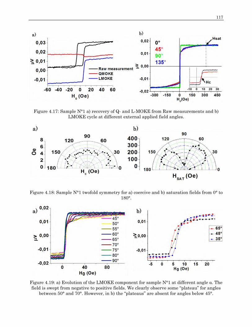
117
Figure 4.17: Sample N°1 a) recovery of Q- and L-MOKE from Raw measurements and b)
LMOKE cycle at different external applied field angles.
Figure 4.18: Sample N°1 twofold symmetry for a) coercive and b) saturation fields from 0° to
180°.
Figure 4.19: a) Evolution of the LMOKE component for sample N°1 at different angle α. The
field is swept from negative to positive fields. We clearly observe some “plateau” for angles
between 50° and 70°. However, in b) the “plateaus” are absent for angles below 45°.

118 Chapter 4: Structural and magnetic properties of “as deposited” CMS Heusler alloys
SAMPLE N°2 :
MOKE measurements have been also performed on sample N°2 only in few directions
and then similar representation of the coercive field or saturation vs. the angle α cannot be
presented. Figure 4.20 shows different raw measurements for different directions of the
applied field 𝛼𝐻 where 0° and 90° corresponds to the easy axis directions of the sample.
Similarly to sample N°1, the cubic anisotropy is observed in the saturation field values at 45°
and 135°. Here the value of the saturation field is evaluated to be around 450 Oe (45 mT).
However, the shape of the hysteresis cycles differs from sample N°1 around the coercive field
value, as shown in the inset of Figure 4.20. Indeed there is a clear difference between the two
easy axes.
In order to compare the different cycles, we applied the symmetric procedure as
explained for sample N°1. The result of the LMOKE signal is shown in Figure 4.21. The field
is scanned from negative to positive values. For 𝛼𝐻=0°, we observe an abrupt decrease of the
magnetization with an almost complete switching, which is typical for an applied field in the
easy axis direction with a corresponding coercive field of 5 Oe (0.5 mT). However for 𝛼𝐻=90°,
we observe that the magnetization amplitude component along the field direction goes down
to zero at µ0H0 = - 2 Oe, so before the direction of the field is reversed. It is followed by a
plateau with a constant value of magnetization until the field is reversed down to the coercive
field of 6.5 Oe. This is typical for the presence of an additional uniaxial anisotropy along the
easy axis 2 (𝛼𝐻 =0°). Indeed, the plateau corresponding to a zero net magnetization means
that the magnetization rotates at 90° from the applied field; i.e. in the easy axis 2 direction.
Similarly to sample N°1, the magnetic switching process for 0° < 𝛼𝐻 < 45° and 45° <
𝛼𝐻< 90° are different. This is observed in Figure 4.22 showing the longitudinal component of
the magnetization for 𝛼𝐻 = 30, 45 and 60°. Typically only for 𝛼𝐻 > 45°, “plateaus” are observed.
Here we have even observed two plateaus before saturation. Once again, this is typical due
to the presence of a uniaxial anisotropy. Details about the switching mechanisms processes
are given in the next sub-section.
Figure 4.20: Hysteresis cycle for sample N°2. The inset shows the difference between two
easy axes (0° and 90°).

119
Figure 4.21: LMOKE cycles after symmetry procedure. The magnetic field is applied in the
four magnetic axes directions.
Figure 4.22: LMOKE measurements at 𝜶𝑯= 30°, 45° and 60° showing different switching
mechanisms.
Switching mechanisms
In order to understand the different magnetic switching mechanisms observed in
samples N°1 and N°2 as a function of 𝛼 , we have simulated the switching process with the
micromagnetic solver OOMMF. Calculations were performed with a 3D package. The size of

120 Chapter 4: Structural and magnetic properties of “as deposited” CMS Heusler alloys
the sample is 2 µm x 2 µm x 40 nm with a cell size of 5 nm. Due to high numbers of cells,
calculations were running using the HPC resources from CALMIP super-calculator in
Toulouse. The easy axes reflecting the cubic anisotropy are the X and Y directions in Figures
4.24 and 4.25. The value of the anisotropy field is set to 𝜇0Hk = 35 mT. Moreover, a uniaxial
anisotropy with amplitude µ0Hu is superposed with the X-axis. The sample is first saturated
with a 100 mT external field applied with an angle 𝛼 with respect to the +X direction. The
field is then decreased in one step down to 20 mT. For the switching process the field is
decreased down to -50 mT by steps of 1 mT and from -50 mT to -100 mT in one step.
Even if the effect of the superposed uniaxial anisotropy is more visible in sample N°2
than in sample N°1, the basic mechanisms are similar. The only difference relies on the
amplitude of the uniaxial anisotropy field µ0Hu which is more important in sample N°2 than
in sample N°1. Here in the simulation we arbitrary set the value 𝜇0Hu = 1 mT, we will see
that this value is in agreement with the one obtained by FMR measurements.
An example of the simulated switching mechanisms for fields applied at 30° or 60°
from the easy axis 1 are presented in figures 4.24 and 4.25 respectively. The basic mechanisms
are the same for every angle of the applied field. We start from saturation in the positive
direction. By decreasing the field, the magnetization first rotates on the edge of the samples,
parallel to the X or Y axis, depending if 𝛼 is inferior or superior to 45°, respectively. This leads
to 90 degrees domain walls as expected in cubic magnetic system. When 𝛼 >45°, the effect of
the additional anisotropy allows for switching of edge domains before the applied field is
reversed. If 𝛼<45°, the magnetization stays in the X direction even at zero field due to the
uniaxial anisotropy.
When the field is reversed (H0 < 0 mT), the situation is first similar whatever the
angle 𝛼. Due to the additional anisotropy in the X direction, the magnetization will form
domains in the center of the sample with magnetization pointing preferentially alternatively
in the + and - X direction (figure 4.24-c and 4.25-c). These domains are separated by cross
ties domain walls as generally observed in soft magnetic systems with thickness around 50
nm. The edge domains are separated from the central domains by 90° domain walls. This
leads to classical flux closure magnetic configuration and corresponds to a net magnetization
equal to zero, i.e. at the coercive field.
Once this magnetic configuration is reached, the situation differs depending if 𝛼 > 45°
or 𝛼 < 45°. If 𝛼 < 45°, the switching occurs through the growing of the central magnetic domain
pointing in the –X direction (Figure 4.24-d). As this direction is the most energetically
favorable due to the uniaxial anisotropy, this process allows for abrupt transition. Then the
saturation is reached with a rotation of the magnetization toward the direction of the applied
field. Now if 𝛼 > 45°, the switching occurs through the propagation of the 90° domain walls in
order to favor domains with magnetization pointing in the –Y direction (see figure 4.25-d and
4.24-e). However, this is energetically less favorable since the uniaxial anisotropy tends to
keep the magnetization in the –X direction. Therefore it is probable that the plateaus
observed for 𝛼 = 60° in figure 4.19 and 4.22 corresponds to the field necessary to move the 90°
domain walls to the center of the sample. Finally saturation is also reached after rotation of
the magnetization toward the direction of the applied field.

121
Figure 4.23: The field is swept from positive to negative fields with steps of 2 mT. The insert
is a zoom around zero field. The additional uniaxial anisotropy is aligned with the easy axis
1 direction, i.e. the +X direction as shown in the scheme on the right.
An example of the simulated hysteresis curves with OOMMF is shown in fig 4.23. The
situation is here similar to what we observe for sample N°2. Indeed, when the field is applied
with α>45°, the average magnetization parallel to the applied field, M, tends to zero before
switching the applied field. This corresponds to the rotation of the magnetization toward the
X direction (the direction of the uniaxial anisotropy). When α< 45° the magnetization still
shows a high value at it is in a stable position.
While we recover also the fact that the saturation is reached at higher field when α>45°, we
observe some plateau for both directions of the applied field. Also the saturation field is almost
an order of magnitude higher than in the experiment. We believe that such discrepancies
comes from the size of the simulated sample. Indeed, as it is only few µm², it is much more
difficult to saturate the edge of the sample due to the local demagnetizing field. This effect is
also present of real samples but as they are mm², edge effects are negligible in the magnetic
response of the sample. The second effect of the size of the simulated sample is a much lower
density of domain walls that can be created to switch the magnetization as compared to real
samples. These two effects naturally increase the saturation fields.
Let’s note that it is very difficult to estimate the value of this uniaxial anisotropy from
the MOKE measurement. Indeed, as the switching occurs through domain wall nucleation
and propagation, no direct value of 𝜇0Hu can be obtained from the measurement of µ0Hc.
Moreover, the amplitude of this anisotropy is much lower than the value of the cubic
anisotropy and it is very difficult to distinguish both contributions in the measurement of the
saturation field within the uncertainty of the measurement. Finally, direct comparison with
micromagnetic simulations is also tricky. Indeed, the measured samples are 3 x 3 mm² while
the simulated sample is 5 x 5 µm². Size effect plays an important role for the value of the
switching field, first because of the effect of the dipolar field and for the nucleation and
propagation of domain walls. Then micro magnetic simulations allow to determine the basic

122 Chapter 4: Structural and magnetic properties of “as deposited” CMS Heusler alloys
mechanisms but don’t give absolute values of the uniaxial field. FMR measurements will show
that this additional anisotropy has an amplitude below 20 Oe.
Figure 4.24: simulated switching mechanisms for fields applied at 30° from the easy axis 1.
Switching from positive b) to negative f) applied field occurs through the growing of the
central magnetic domain pointing in the –X direction as shown in c), d) and e).
Finally, we need to discuss the origin of the additional uniaxial anisotropy. Up to now
there is no clear explanation for it. In a previous work [11 Ortiz], we suggested that uniaxial
anisotropy in CMS deposited on MgO could originate from the presence of terraces on the
surface of MgO substrate crystals. Indeed, some studies suggest that nanometer-scale steps
in MgO substrate induce an in-plane magnetic easy direction perpendicular to the step edge.
This effect was also accounted for the uniaxial anisotropy in Fe3O4//MgO(001) [12 McGuigan],
Fe//W(001), [13 Chen], Fe//Ag(001), and Fe//Au(001) thin films [14 Leeb]. The mentioned
references, [12-14], suggested that the origin of this magnetic anisotropy can arise from the
preferential alignment of structural defects with step edges. While Leeb et al. pointed out that
the magnitude of the magnetic anisotropy is determined by the large lattice out-of-plane
mismatch which gives rise to strong strain in the vicinity of monoatomic steps.

123
Figure 4.25: simulated switching mechanisms for an external field applied at 60° from the
easy axis 1. The switching occurs through the propagation of the 90° domain walls in order
to favor domains with magnetization pointing in the negative Y direction as shown in d) and
e).
Additionally, the lattice mismatch between the substrate and the thin films is often
accounted for a tetragonal distortion of the cell, with the product a²c constant (iso-volume
distortion), inducing strain anisotropy. This strain anisotropy has been often considered as
the origin of the superposed magnetic uniaxial anisotropy observed in many cubic systems.
The uniaxial anisotropy has been found to be either in one of the cubic easy axis direction, for
example in Co2FeAl [16 Belmeguenai], or in one of the cubic hard axis, for example in Iron
[15 Baker]. However, Pandey et al. [3, 17 Pandey] have recently studied the magneto elastic
anisotropy induced by lattice mismatch for thin films of CMS deposited on either MgO or STO
substrate. In their work they observe a clear out of plane anisotropy induced in the CMS
deposited on STO, but no significant magneto-elastic anisotropy is induced for CMS deposited
on MgO.
As demonstrated by X-ray diffraction, our samples show also a tetragonal distortion which
could be the origin of the uniaxial anisotropy in our sample. Even if our films are completely
relaxed, we will see that FMR measurements prove this superposed uniaxial anisotropy. In
the next chapter, we will show that ion irradiation increases the out of plane deformation of
the alloy which goes along an increased amplitude and a rotation of the uniaxial anisotropy,
supporting the idea that the tetragonal distortion is at the orgin of the uniaxial anisotropy.

124 Chapter 4: Structural and magnetic properties of “as deposited” CMS Heusler alloys
4.2.2 Domain walls observation by Lorentz microscopy
As presented in chapter 3, Lorentz microscopy is a powerful tool to image and study
the geometry of domain and domain walls in a ferromagnetic material. Here we apply this
technique to study the shape of the domain walls in the CMS samples and verify the validity
of the switching mechanisms presented in the previous section.
Experiments were carried out at the CEMES laboratory by Dr. Luis Alfredo Rodriguez
using Hitachi HF-3300 (I2TEM-Toulouse) microscope operated at 300 kV. The I2TEM
microscope is especially dedicated to study magnetic samples by electron holography and
Lorentz microscopy. It is equipped with an image corrector (CEOS B-COR) to correct off-axial
aberrations and has a cold field emission gun that emits highly coherent electrons with a very
high brightness of about ~ 107 A/cm2.sr. These two features allow resolving magnetic contrasts
with a very good signal-to-noise ratio. Examples of TEM Lorentz mode images are presented
in Figure 4.25 for sample N°3.
This sample has been dedicated to this experiment and prepared for an in-plane view
sample preparation. We note that, no magnetic field has been applied prior to the observation,
so it is observed as inserted in the TEM sample holder. As explained in chapter 3, contrasts
due to domain walls can be observed when defocusing the image as shown in Figure 4.25-b
and 4.25-c. Clearly we observe the different features predicted by micromagnetic simulations.
Indeed, we observe mainly 90° domain walls, especially close from the edge of the central hole
(this is done to decrease locally the thickness of the sample so the incoming electrons are able
to penetrate the material). Moreover, we also observe some particular contrast as shown in
Figure 4.25-c corresponding to a zoom of the yellow box in Figure 4.25-b. Here we recognize
the cross-tie domain walls which appear around the coercive field in the MOKE experiments.
Figure 4.25: Low-magnification Lorentz images for the sample N°3 recorded at a) in-focus and
b) out-of-focus conditions. In c), a zoom image of b) to observe the exotic magnetic contrast
(yellow box). The intensity contrast has been forced in the defocus images to enhance the
visualization of DWs. The yellow arrows show the direction of the magnetization deduced
from the out of focus image in the different domains.
A closer look of the cross-tie domain wall is presented in Figure 4.26. They can be understood
as a succession of vortex states with the same polarity and chirality. The white contrast
observed in Figure 4.26-a. corresponds to the zone for which spins of two surrounding vortices

125
rotates in opposite direction. In this part, the Y component of the magnetization points either
in the + or – direction leading to a difference of contrast as sketched in Figure 4.26-d.
Figure 4.26: (a) Defocus image recorded around a complex DW configuration. (b) Magnetic
color map of (a) by solving TIE. White arrows represent the average magnetization orientation
of each domain. (c) A zoom of the yellow box in (b) where white lines represent the magnetic
flux. (d) A simple cartoon representing the magnetic structure of the DW. Color arrows
represent the local magnetization orientation while bright/dark lines and dark spots
correspond to the magnetic contrast observed in the defocus image. e) OOMMF simulations
of cross tie domain walls.
4.2.3 FMR Dynamic properties measurements
Ferromagnetic Resonance (FMR) is a common and powerful technique which is
used to extract the magnetic parameters of a ferromagnetic material. In this
section we will present the different geometry used in this work to extract the
magnetization, the gyromagnetic ratio, the anisotropy and the exchange values
of the three samples. Then we will present the measurement of the linewidth and
discuss the value of the Gilbert damping extracted from the FMR.

126 Chapter 4: Structural and magnetic properties of “as deposited” CMS Heusler alloys
4.2.3.1 Extraction of magnetic parameters.
Methodology:
As presented in chapter III, in our FMR set-up, a microwave voltage is injected in the
stripline and a modulation technique is used to measure the absorbed power signal by the
magnetic film placed on the stripline. This technique allows for a direct inductive coupling
between the stripline and the sample. The lateral dimensions of the studied samples range
between 4*4 for samples of series N°1 and 3*3 mm² for series N°2 and N°3. These dimensions
are bigger than the stripline width (400 µm). This leads to a non-uniform excitation field and
thus we are not in a pure FMR geometry where the microwave excitation field is uniform over
the sample. Indeed, we are in a configuration of surface spin waves excitation. However,
considering the maximum wave vector that can be excited k=2π/L with L = 400 µm, and taking
into account the corrections to the FMR frequency (chapter 2 equation 2.78), we find that that
the effect of the finite size of the stripline shifts the resonance frequency by an amount of
approximately 4 MHz which corresponds to a field shift of about 0.2 mT. Such a shift value is
below the uncertainty of our measurement which is about 0.3 mT. Therefore, considering a
uniform mode, formulas 2.54 to 2.56 will be applied to recover the magnetic parameters of the
samples.
A typical FMR spectrum for different excitation frequencies is presented in Figure
4.27. The magnetic field is scanned from 0 to 450 mT. We can see that the signal corresponds
to the derivative of the imaginary part of the susceptibility. However, and as explained
previously, signals always contain a small contribution from the real part of the susceptibility
due to the sample length, allowing for a small propagation effect, and also because the
propagating mode of the stripline is not purely TEM. Then our data are fitted with a function
of the form:
𝑌 ∝ 𝑐𝑠𝑡 +𝑑𝜒′
𝑑𝐻cos𝜑 +
𝑑𝜒′′
𝑑𝐻sin 𝜑 (4.14)
With φ an arbitrary dephasing angle and 𝜒 =𝑐𝑠𝑡
(𝛾𝐻0−𝛾𝐻𝑟𝑒𝑠)−𝑖𝛼(𝛾Δ𝐻
2𝛼)= 𝜒′ + 𝑖𝜒′′ =
𝑐𝑠𝑡(𝐻−𝐻𝑟𝑒𝑠)
(𝐻−𝐻𝑟𝑒𝑠)2+(
Δ𝐻
2)2+
𝑖𝑐𝑠𝑡(
Δ𝐻
2)
(𝐻−𝐻𝑟𝑒𝑠)2+(
Δ𝐻
2)2
It can be seen in figure 4.27 that the angle φ, in this case, is very small ( < 10°). The
Symbols correspond to experimental data, while the full lines are the fit obtained from
equation 4.14. From the fit we are able to deduce the value of the applied field at the resonance
as well as the linewidth of the signal ΔH which allows to study the relaxation parameters,
that will be presented in section 4.2.3.2. Interestingly, we will show that the different CMS
samples studied in this manuscript show some clear asymmetry of the resonance peaks due
to multiple resonance with very close resonance fields and linewidths.

127
Figure 4.27: A typical FMR spectra at different frequencies.
In our work, FMR measurements have been performed in different geometries
depending on the applied magnetic field orientation with respect to the film’s surface. In the
first case, the external magnetic field is applied in the plane of the sample (i.e. 𝜃𝐻 = 90°). The
maximum external field can reach about 450 mT and the air gap is 8 cm. In this geometry the
external field has been applied in either the easy or hard axes directions for measurements
of Hres vs. fres (Figure 4.28-a). For this measurement the sample is rotated and the
electromagnet is kept at a fixed angle with respect to the sample holder. It allows staying
always in the “Surface Spin Waves configuration”. We also performed measurements of the
resonance field Hres as a function of the angle 𝜑𝐻 of the external field with respect with one
easy axis at constant excitation frequency (Figure 4.28-b). In the latter, the electromagnet is
rotated with respect to the sample holder with a relative angle variation between 0 and 180°.
Let’s note that when φ𝐻~ 90°, we are in the Magnetostatic Backward Volume Waves
(MSBVW) configuration. However, here also the field shift due to MSBVW is close to 0 MHz.
Moreover, we verified that we observe the same resonance field if φ𝐻 =90° or if φ𝐻=0° when
the sample is rotated by 90°. The only difference relies on the measured amplitude signal
which is much smaller if φ𝐻 = 90° as the pumping field is parallel to the magnetization.
In the second experimental geometry, the field is applied perpendicular to the plane
of the layer (i.e. 𝜃𝐻 = 0°). An example of such measurement is presented in Figure 4.28-c). In
this configuration, we modify the poles of the electromagnet so the magnetic field can reach a
value of 1.6 T and the air gap is decreased to 2 cm.
By fitting all the different dispersion relations fres vs. µ0H0 and Hres vs. φ, we were
able to extract the values of the gyromagnetic ratio 𝛾/2𝜋, the magnetization µ0Ms and the
anisotropy field µ0Hk. The latter parameter being the simplest one to determine as it
corresponds to the inflexion point in the fres s. µ0H0 curve in the in-plane hard axis direction
(figure 4.28 a).

128 Chapter 4: Structural and magnetic properties of “as deposited” CMS Heusler alloys
Figure 4.28: Example of measurements for the different experimental configurations used in
this work. In a), dispersion relation fres vs. 𝜇0H0 for in-plane measurements. The points
corresponds to experimental data and the solid lines to the fit using equations 2.54 and
2.55. b), FMR angular measurements of 𝜇0H0 vs. 𝜑 at 13 GHz. c) Out-of-plane
measurements of fres vs. 𝜇0H0. The line corresponds to the fit using equation 2.56.
We will now present the results of FMR spectra for the reference samples of the three series
and try to correlate the magnetic properties to the structural analysis presented in sections
4.1.2 and 4.1.3.
Sample N°1:
Two examples of recorded absorption spectra are shown in Figure 4.29. The first one
presents the FMR signal for an applied field parallel to the easy axes, i. e. [110] and [110],
(Fig. 4.29-b) while the second one corresponds to an applied field parallel to the hard axes, i.
e. [100] and [010] (Fig. 4.29-c). The excitation frequency field is 16 GHz for all those mentioned
spectra measurements.
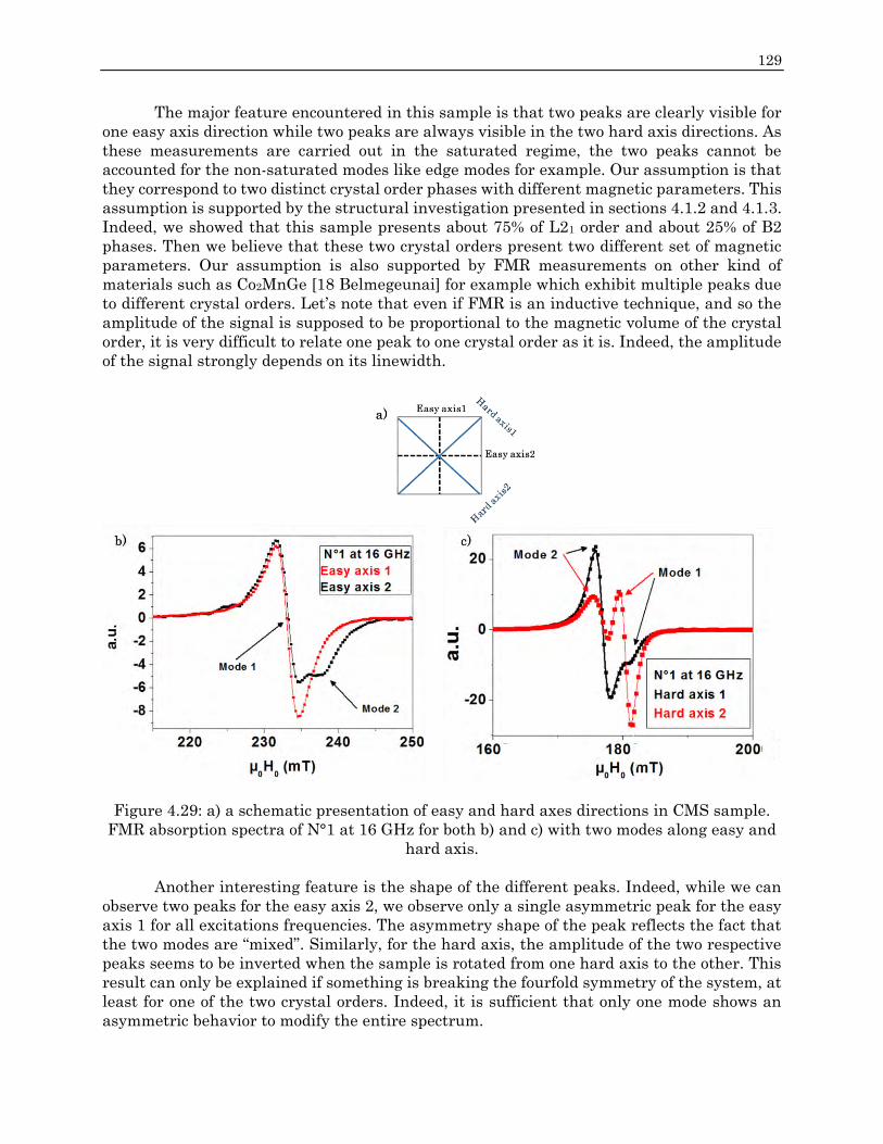
129
The major feature encountered in this sample is that two peaks are clearly visible for
one easy axis direction while two peaks are always visible in the two hard axis directions. As
these measurements are carried out in the saturated regime, the two peaks cannot be
accounted for the non-saturated modes like edge modes for example. Our assumption is that
they correspond to two distinct crystal order phases with different magnetic parameters. This
assumption is supported by the structural investigation presented in sections 4.1.2 and 4.1.3.
Indeed, we showed that this sample presents about 75% of L21 order and about 25% of B2
phases. Then we believe that these two crystal orders present two different set of magnetic
parameters. Our assumption is also supported by FMR measurements on other kind of
materials such as Co2MnGe [18 Belmegeunai] for example which exhibit multiple peaks due
to different crystal orders. Let’s note that even if FMR is an inductive technique, and so the
amplitude of the signal is supposed to be proportional to the magnetic volume of the crystal
order, it is very difficult to relate one peak to one crystal order as it is. Indeed, the amplitude
of the signal strongly depends on its linewidth.
Figure 4.29: a) a schematic presentation of easy and hard axes directions in CMS sample.
FMR absorption spectra of N°1 at 16 GHz for both b) and c) with two modes along easy and
hard axis.
Another interesting feature is the shape of the different peaks. Indeed, while we can
observe two peaks for the easy axis 2, we observe only a single asymmetric peak for the easy
axis 1 for all excitations frequencies. The asymmetry shape of the peak reflects the fact that
the two modes are “mixed”. Similarly, for the hard axis, the amplitude of the two respective
peaks seems to be inverted when the sample is rotated from one hard axis to the other. This
result can only be explained if something is breaking the fourfold symmetry of the system, at
least for one of the two crystal orders. Indeed, it is sufficient that only one mode shows an
asymmetric behavior to modify the entire spectrum.

130 Chapter 4: Structural and magnetic properties of “as deposited” CMS Heusler alloys
Naturally, one can think about the uniaxial anisotropy detected by MOKE
measurements. If the anisotropy is aligned with the easy axes, one expects a shift of the
resonance fields between the two easy axes while the FMR signals in the hard axes are at the
same positions. This is what we observe, within the uncertainty of our measurement, a shift
in the easy axis resonance at least for the mode 2 as shown in figure 4.30.
Moreover, another difference we observe when fitting the experimental data, is
that the amplitude of the different peaks are always different. For example, the
amplitude ratio of the primary peak/ secondary peak in the fitted curves has a value
of 1.5 in figure 4.30-a) and 6 for the blue fitted curve in 4.30-b. Despite different
amplitude ratios depending on the orientation of the field, we always observe a peak
with lower amplitude in agreement with the fact that we have different crystal order
in the sample with different volume. Therefore we believe that the two resonance modes
exhibit anisotropy of the linewidth as a function of the direction of the applied field. This
effect is expected in crystals as the damping tensor reflects the symmetry of the system.
However the two hard axes on one hand and the two easy axes on the other hand should be
equivalent. Here, we believe that the relaxation differs for every direction of the applied field.
We will develop this point in the next subsection 4.2.3.2 devoted to the damping and
relaxation mechanisms.
Let’s note that it is more difficult to define the value of the linewidth for each mode
when the field is applied in the easy axis 1. Indeed we show in Figure 4.30-b two examples
(red and blue lines) of simulated signals which are in very good agreement with the
experimental data. While the resonance fields are the same as for the easy 1, the amplitude
and linewidths of the two modes are different, especially for mode 2. Then it is extremely
difficult to get a precise measurement of the linewidth of the two modes if the peaks are not
sufficiently resolved. To show how much the two peaks are mixed, we also fitted this curve
with a single peak (green line), and the agreement is also very good. However the dephasing
between the real and imaginary part φ reaches 18°, which is quite important. This is why we
can state that when a peak is very asymmetric, it contains most probably two resonant modes.
The situation is quite similar when the field is applied in the hard axis 1 direction. Even if
the mode 1 is clearly visible, it is very difficult to determine with a good precision the value
of the linewidth if the peak is not well resolved.

131
Figure 4.30: absorption spectra at 16 GHz as a function of external field for CMS N°1 along
the two easy axes in a) and b) and the two hard axes in c). Experimental data are presented
as points and the solid lines correspond to linear fit with different adjustment parameters
using equation 4.14.
In order to determine the magnetic parameters corresponding to the two modes, we
use the spectra for which the peaks are well resolved. The evolution of the resonance field as
a function of frequency for in-plane and out-of-plane configuration are presented in Figure
4.31-a) and 4.31-d, respectively. Only one easy and one hard axes are drawn here. Figure
4.31-b is a zoom on the black box in Figure 4.31-a, to show the small difference between the
two phases. Figure 4.31-c corresponds to the angle measurement of the resonant field as a
function of the in-plane angle between the applied field and the easy axis at 13 GHz. The solid
lines in the different curves correspond to the adjustment using equations 2.54 to 2.56.
In figure 4.31-a, we also show the first standing spin wave modes (SSW) measured in
the direction of the easy axis 1 and hard axis 1 direction. This mode is an exchange dominated
excitation in the thickness of the layer that appears at lower magnetic fields than the uniform
mode as shown in Figure 4.31-e. It allows to extract the value of the exchange constant, A,
Indeed, in the in-plane configuration and for an external field applied either parallel to the
easy or hard axis, the dispersion relation that relates the resonance frequency of the SSW to
the applied field (following equation 2.85 in chapter 2) is expressed as:
SSW Easy axis: 𝒇𝒓𝒆𝒔 =𝝁𝟎𝜸
𝟐𝝅[(𝑯𝟎 +𝑯𝒌 +
𝟐𝑨
𝝁𝟎𝑴𝒔𝒌𝒛,𝒏𝟐 ) (𝑯𝟎 −
𝑯𝒌
𝟐+
𝟐𝑨
𝝁𝟎𝑴𝒔𝒌𝒛,𝒏𝟐 +𝑴𝒔)]
𝟏/𝟐 (4.15)
SSW Hard axis: 𝒇𝒓𝒆𝒔 =𝝁𝟎𝜸
𝟐𝝅[(𝑯𝟎 −𝑯𝒌 +
𝟐𝑨
𝝁𝟎𝑴𝒔𝒌𝒛,𝒏𝟐 ) (𝑯𝟎 −𝑯𝒌 +
𝟐𝑨
𝝁𝟎𝑴𝒔𝒌𝒛,𝒏𝟐 +𝑴𝒔)]
𝟏/𝟐 (4.16)

132 Chapter 4: Structural and magnetic properties of “as deposited” CMS Heusler alloys
Where 𝒌𝒛,𝒏𝟐 =
𝒏𝝅
𝒅, with 𝒅 being the thickness of the CMS layer (≈42 ±1 nm), n corresponds to
the pinning mode and A is the exchange stiffness constant. To calculate the exchange value,
we consider the first excitation mode with n=1. Moreover we consider a perfect pinning at the
surfaces. These assumptions are supported by the fact that, even if the film thickness is well
below the skin depth, the amplitude of the microwave field is slightly different between the
two surfaces of the sample. The pumping field being non-uniform in the thickness of the layer,
it allows for the excitation of the first mode. Rigorously, the pinning parameters p and the
mode index n in equation 2.84 could be determined if we could have observed at least 3
standing spin waves modes [19 Wigen]. However, the frequencies of the modes with n>1 are
higher than 30 GHz, the limit of our microwave source. Finally, as the signal is very small it
is impossible to distinguish the contribution of the two respective phases and the exchange
value is calculated considering the parameters of mode 1.
The deduced parameters for µ0Ms, µ0Hk, the gyromagnetic ratio 𝛾/2𝜋 and the
exchange value A are presented in table 4.4. We obtain very similar values of the magnetic
parameters for each mode observed in the FMR spectrum. First the magnetization values are
very close from the theoretical prediction. Taking into account the lattice parameters obtained
by X-ray diffraction, we get 4.88 and 4.85 𝜇𝐵/𝑓. 𝑢 for modes 1 and 2 respectively, to compare
with the theoretical prediction of 5 µB for perfect L21 or B2 structure. This result is also in
very good agreement with the structural studies. Then we attribute the two resonance modes
to the B2 and L21 crystal order. The small decrease of the magnetic moment as compared to
theoretical value is most probably due to a small amount of Co-Si exchange in each phase (we
remind that the Co/Si exchange parameters has been found to be around 0.04 for this sample).
We confirm the average value of the magnetization with PPMS measurement (Figure 4.32).
We obtain average magnetization amplitude of 1.26 ± 0.02 T for CMS Heusler alloy. The
uncertainty on the PPMS measurement is due to the uncertainty on the exact dimension of
the sample.
The main difference between the two modes concerns the anisotropy. First we
succeeded to fit the angle dependence of the resonant field of mode 2 taking into account a
very small uniaxial anisotropy of µ0Hu ~0.9 mT in the easy axis 2 direction, as expected from
MOKE measurement. This superposed anisotropy seems to be absent for mode 1. In order to
fit this uniaxial anisotropy for mode 2, we include in the calculation of the total energy of the
system a term of the form Ku.Sin²(𝛽), with 𝛽 the angle of the magnetization with respect to
easy axis 1.
We also deduced cubic anisotropy values which are more important than the values
generally reported for CMS deposited on MgO, for example, [20 Yilgin, 21 Gaier] but
equivalent to the ones previously reported by Ortiz et al. This can be related to the deduced
value of the g factor calculated from g =𝜸∗𝟐𝒎𝒆
|𝒆|. Indeed we obtain values of g ≈ 2.05 (considering
the mass of a free electron) for both modes. This value is in agreement with reported values
in literature for CMS ([4 Belmeguenai, 2 Rameev, 23 Hamrle and 1 Ortiz]) of 2.05 or 2.04.

133
Figure 4.31: Dispersion relation fres vs. µ0H0 in CMS N°1 for a) in-plane and d) out-of-plane
configuration. Figure b) corresponds to a zoom on the two modes for the black box in a). c)
Angular dependence of the resonance field at 13 GHz. e) FMR signal at 22 GHz in the easy
direction showing both the FMR and SSW modes.
According to the Kittel formalism for ferromagnetic material with small orbital
moment, 𝑔 can be related to the ratio of orbital over spin moment such as (g − 2) = 2 (µL
µs).
Then we believe that our sample shows a small contribution from orbital moment. As the
anisotropy relates the orbital and spin moment through the spin-orbit coupling, the orbital

134 Chapter 4: Structural and magnetic properties of “as deposited” CMS Heusler alloys
contribution is maybe the origin of the large value of the cubic anisotropy. This assumption
will be supported by the effect of ion irradiation on the cubic anisotropy in chapter V.
Moreover, the slightly lower value of the anisotropy constant for the mode 2 could be expected
in the B2 phase due to the disorder on the Mn and Si sites which change the local environment
of the Mn atoms carrying most of the magnetic moment. Therefore, we attribute the mode 2
to the B2 order and the mode 1 to the L21 order. Further study of the FMR linewidth (see next
subsection) wil support this assumption.
Finally, we found a value of the exchange constant, A, close to the values reported in
literature for L21 structure. Indeed the exchange constant is found to range between 19 and
23 pJ/m as mentioned in [24 Ritchie, 23 Hamrle and 3 Pandey]. This exchange constant value
is in a good agreement with the values of the magnetization. Indeed the magnetization
depends on the splitting of spin up and down energy states which is related to the strength of
the exchange spitting.
CMS
sample
N°1
Magnetization
saturation Ms
(T)
Anisotropy
field Hk
(mT)
Anisotropy
constant
Kc=𝑯𝑲∗𝝁𝟎𝑴𝒔
𝟐
(KJ/m3)
Uniaxial
Anisotropy
field (mT)
Gyromagnetic
ratio 𝛾
2𝝅
(GHz/T)
Exchange
constant
A (PJ/m)
Phase
1
1.26 ±0.02 36±0.2 -18.042±0.2 28.7±0.1 19±0.5
Phase
2
1.25 ±0.02 33±0.2 -16.91±0.2 0.9 28.7±0.1
Table 4.4: Magnetic parameters of the CMS reference sample N°1 for the two phase measured
by FMR.
Figure 4.32: PPMS measurements on CMS N°1 with an average magnetization of 1.26 T.
Sample N°2:
Similar treatment has been conducted on sample N°2. Examples of the different
measurements are shown in Figure 4.33. For this sample we were only able to distinguish
one resonance peak. However, we still notice an asymmetry of the peak shape which could
mean that we have two modes with very similar magnetic parameters that are mixed in the

135
measured spectra. We also note a small shift of the resonant field of 1.7 mT for the easy axis
2. This shift does not exist for the hard axes (within the precision of the alignment of the
applied field with respect to the hard axis, which is less than 1°). This means that we have a
uniaxial anisotropy superposed to the easy axis 2, confirming the MOKE experiment. The
presence of the additional uniaxial anisotropy allows fitting the angle dependence of the
resonance field as a function of the angle φ (Figure 4.33-e).
Figure 4.33: FMR absorption spectra for CMS N°2 for in-plane configuration along a) easy
axes at 18 GHz and b) hard axes at 17 GHz. fres vs 𝝁𝟎H0 for c) in-plane and d) out-of-plane
configurations. In e), angular dependence of resonance fields at 20 GHz.
The magnetic parameters extracted from the simulation are presented in table 4.5. The
amplitude of the uniaxial anisotropy µ0Hu is found to be about 1.5 mT. While we observe the

136 Chapter 4: Structural and magnetic properties of “as deposited” CMS Heusler alloys
same value of gyromagnetic ratio as for sample N°1, the cubic anisotropy constant is much
higher while the exchange constant is almost half of sample N°1. It is surprising to have an
increased value of the cubic anisotropy without any change of the gyromagnetic ratio. The
value of the gyromagnetic ratio 𝛾/2𝜋 means that the amplitude of the orbital and spin moment
are similar to sample N°1. The increased cubic anisotropy signifies an increased spin orbit
interaction. Then it is most probably the value of the spin orbit constant, λSO, which must
differ from sample N°1.
Moreover, the magnetization amplitude and exchange constant are found to be lower
than for the sample N°1. Even if no quantitative study of atomic disorder have been conducted
on this sample we already stated that it shows some degree of L21 order but Co/Mn, Co/Si and
Mn/Si exchanges are fairly to be considered. Dealing with the Mn/Si disorder (B2 type
disorder), Gaier et al. have obtained an exchange value of 18 pJ/m for the pure B2 phase.
Therefore, we assume the reduced value of the magnetization and exchange amplitudes to be
related to an important Co/Mn and/or Co/Si disorders.
Magnetizati
on
saturation
Ms (T)
Anisotropy
field Hk
(mT)
Anisotropy
constant
Kc=𝑯𝑲∗𝝁𝟎𝑴𝒔
𝟐
(KJ/m3)
Uniaxial
anisotropy
field Hu
(mT)
Gyromagnet
ic ratio 𝛾
2𝝅
(GHz/T)
Exchange
constant
A (PJ/m)
CMS
sample
N°2 1.24 ±0.02 53±0.2 -26.14±0.2 1.5±0.2 28.8±0.1 10±0.5
Table 4.5: Magnetic parameters of sample N°2 deduced from FMR measurements presented
in figure 4.33.
Sample N°3:
The situation for sample N°3 is somewhere between samples N°1 and N°2. Indeed, as
shown in Figure 4.34-a and 4.34-b, two modes are visible for the applied field parallel to the
hard 2 direction while it is barely visible above 19 GHz in the easy axis 1 direction. For the
two other magnetic directions only a single resonance peak is observed.
The main difference with sample N°1 is that not only the amplitude of the peaks
change when going from the hard axis 1 to the hard axis 2, but also the position of the peaks
with a clear shift of mode 1 of about 5 mT at 19 GHz. Even if HAADF-STEM only shows L21
order for this sample, we believe that it most probably shows some inclusions of B2 order in
the matrix. The L21 order being clearly predominant over the B2 phase in terms of volume.
Due to the difficulty to separate both contributions in the FMR spectra (except for the hard
axis 2), only the magnetic parameters will be extracted for the main mode corresponding to
the L21 phase.
Once again, the shift of resonance field when going from one hard axis to the other can
be explained by the presence of an additional uniaxial anisotropy. However this time it is
superposed with the hard axis 1 (let’s note that most probably the minority mode shows no
additional anisotropy). Our assumption is also supported by angle measurements that are
perfectly fitted considering the main mode with a superposed uniaxial anisotropy (figure 34-
d) in the hard axis 1 direction. As already mentioned, tetragonal distortion of the cell has been

137
proved to induce such kind of anisotropy in Iron for example in the case of doping with Dy
atoms. This situation is different from sample N°1 and N°2 for which we observed a uniaxial
anisotropy superposed to the easy axis. The first explanation for this difference could be the
amplitude of the out of plane lattice parameter which is higher for the sample N°3 than for
sample N°1. Another possibility relies on the nature of the atomic plane being either the Co
planes or the Mn-Si planes in contact with the MgO substrate. However, further structural
characterization studies would be necessary to clarify this point.
The values for the different magnetic parameters obtained from the different fits are
presented in table 4.6. The cubic anisotropy, exchange and gyromagnetic factor values are
similar to sample N°1 while the magnetization is slightly lower. This can be due to the higher
Co-Si exchange deduced from by X-ray diffraction with Cu source.
Figure 4.34: FMR absorption spectra for CMS N°3 for in-plane configuration along a) easy
axes and b) hard axes at 19 GHz. c) fres vs. H0 for in-plane SSW and uniform mode
configurations. In d), angular dependence of resonance fields at 13 GHz.
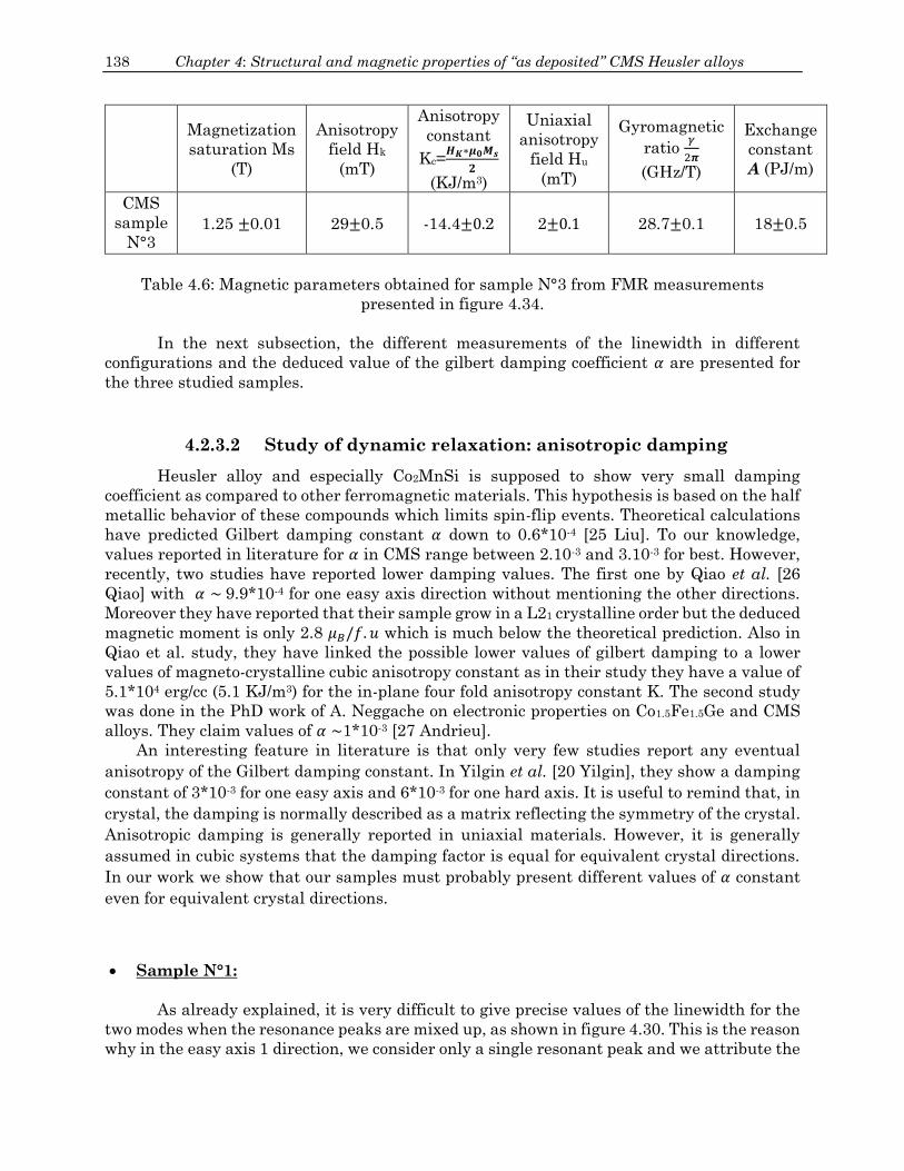
138 Chapter 4: Structural and magnetic properties of “as deposited” CMS Heusler alloys
Magnetization
saturation Ms
(T)
Anisotropy
field Hk
(mT)
Anisotropy
constant
Kc=𝑯𝑲∗𝝁𝟎𝑴𝒔
𝟐
(KJ/m3)
Uniaxial
anisotropy
field Hu
(mT)
Gyromagnetic
ratio 𝛾
2𝝅
(GHz/T)
Exchange
constant
A (PJ/m)
CMS
sample
N°3 1.25 ±0.01 29±0.5 -14.4±0.2 2±0.1 28.7±0.1 18±0.5
Table 4.6: Magnetic parameters obtained for sample N°3 from FMR measurements
presented in figure 4.34.
In the next subsection, the different measurements of the linewidth in different
configurations and the deduced value of the gilbert damping coefficient 𝛼 are presented for
the three studied samples.
4.2.3.2 Study of dynamic relaxation: anisotropic damping
Heusler alloy and especially Co2MnSi is supposed to show very small damping
coefficient as compared to other ferromagnetic materials. This hypothesis is based on the half
metallic behavior of these compounds which limits spin-flip events. Theoretical calculations
have predicted Gilbert damping constant 𝛼 down to 0.6*10-4 [25 Liu]. To our knowledge,
values reported in literature for 𝛼 in CMS range between 2.10-3 and 3.10-3 for best. However,
recently, two studies have reported lower damping values. The first one by Qiao et al. [26
Qiao] with 𝛼 ~ 9.9*10-4 for one easy axis direction without mentioning the other directions.
Moreover they have reported that their sample grow in a L21 crystalline order but the deduced
magnetic moment is only 2.8 𝜇𝐵/𝑓. 𝑢 which is much below the theoretical prediction. Also in
Qiao et al. study, they have linked the possible lower values of gilbert damping to a lower
values of magneto-crystalline cubic anisotropy constant as in their study they have a value of
5.1*104 erg/cc (5.1 KJ/m3) for the in-plane four fold anisotropy constant K. The second study
was done in the PhD work of A. Neggache on electronic properties on Co1.5Fe1.5Ge and CMS
alloys. They claim values of 𝛼 ~1*10-3 [27 Andrieu].
An interesting feature in literature is that only very few studies report any eventual
anisotropy of the Gilbert damping constant. In Yilgin et al. [20 Yilgin], they show a damping
constant of 3*10-3 for one easy axis and 6*10-3 for one hard axis. It is useful to remind that, in
crystal, the damping is normally described as a matrix reflecting the symmetry of the crystal.
Anisotropic damping is generally reported in uniaxial materials. However, it is generally
assumed in cubic systems that the damping factor is equal for equivalent crystal directions.
In our work we show that our samples must probably present different values of 𝛼 constant
even for equivalent crystal directions.
Sample N°1:
As already explained, it is very difficult to give precise values of the linewidth for the
two modes when the resonance peaks are mixed up, as shown in figure 4.30. This is the reason
why in the easy axis 1 direction, we consider only a single resonant peak and we attribute the

139
linewidth to the mode 1 (which will be shown to correspond to the most predominant L21
order). In addition, the mixing of the two peaks makes difficult the measurement of the
linewidth in the hard axis 1 direction for the mode 1, as can be seen by the strong variations
of the green dots in figure 4.35 c. Then for this crystal direction we do not give value of the
damping coefficient of the mode 1. Also we do not present the linewidth of the two modes for
the out of plane configuration due to the small number of point measured in the saturated
regime as shown in Figure 4.28-e.
Figure 4.35: line width measurements as a function of the applied frequency along easy and
hard axes for the two observed L21 and B2 phases of sample N°1. In a) and b) the two modes
are distinguished for easy 2 and hard 2 axes, respectively. While in c) and d), line width
values (∆𝑯) of L21 and B2 phases and their linear fit are traced for each easy and hard axis
showing their corresponding damping coefficient 𝜶 and ∆𝑯𝟎.
In Figure 4.35-a) and 4.35-b we compare the linewidth of the two resonance peaks
measured either in the 2 easy or in the 2 hard directions. Clearly, the mode 1 shows lower
values of the linewidths than the mode 2, reinforcing the idea that the mode 1 corresponds to
the L21 order and the mode 2 to the B2, as the latter grows in the form of crystallites in the
L21 matrix. Then in the following we will consider the two peaks to correspond to the L21 and
B2 modes and we will refer the mode 1 as the L21 mode and the mode 2 as the B2 mode.
The linewidths in the different directions of the crystal are presented in figure 4.35-c
for the L21 mode and in figure 4.35-d for the B2 mode. For both modes, it appears that the
linewidth amplitudes depend on the direction of the applied field. However, for both the L21
and B2 modes, it appears that the damping coefficient is roughly constant for each direction.

140 Chapter 4: Structural and magnetic properties of “as deposited” CMS Heusler alloys
Then the difference in the linewidth seems to be essentially related to the variation of the
extrinsic contributions ΔH0. Indeed, for the L21 order, the 𝛼 value is equivalent for the easy
axis 2 and the hard axis 2. We found values of 1.5 and 1.6*10-3 ± 0.1*10-3, respectively. These
values are very good with respect to other reported values for CMS and are similar to the ones
reported for Co2FeAl [16 Belmeguenai]. In the hard axis 1, the dispersion is pretty important
which avoids a precise value of 𝛼. Finally, 𝛼 is found to increase for the easy axis 1 with a
value of about 2.1*10-3. The difference between the two easy axes is most probably due to the
fact that in the easy axis 1 direction, the L21 and B2 peaks are hardly dissociated and then it
naturally increases the measured linewidth. Similarly, the 𝛼 value for the B2 order in the
easy axis 2 appears to be higher than for the hard axes. However, we can see in Figure 4.35-
c that the dispersion in the experimental data is very important as the amplitude of the peak
in the FMR signal is weak and mixed up with the L21 mode. Then it is difficult to clearly state
about a potential anisotropic behavior of 𝛼 in the B2 order. In conclusion, from these
measurements, we do not observe neither the expected cubic symmetry nor a clear difference
between the damping coefficient in the easy and hard axis directions, as reported by others.
Further insight can be obtained from the evolution of the linewidth as a function of the
in plane angle φ of the applied field (φ scan) presented in figure 4.36-c and 4.36-d for the L21
and B2 modes, respectively. The determination of the exact value in this configuration is very
difficult for two reasons. As both peaks does not show the same dependence with the angle φ
(as shown by the simulations in Figure 4.31-c), the mixing of the mode and then uncertainty
on the linewidth values, is reinforced for most of the angle φ. The second reason is due to the
decrease of signal amplitude with φ. Indeed, in these measurements we change the
orientation of the field as sketched in the figure 4.36. As already stated, the microwave
magnetic field generated by the stripline turns from the magnetization perpendicular to
parallel when φ = 90°. This last configuration corresponds to the excitation of backward
volume waves and the coupling between the microwave field and the magnetization is
minimum. An example of such effect is shown in fig 4.36-a. Then it becomes very complicated
to get a precise measurement of the different linewidth when the signal is almost of the order
of the experimental noise.
Despite the experimental limitations, we clearly observe some variations of the
linewidth as a function of φ for both modes. In principle, the linewidth as a function of φ is
supposed to reflect the cubic anisotropy [16 Belmeguenai] due to the 𝜕𝑓
𝜕𝐻 term in equation 2.38.
For the L21 mode, we observe two minima of the linewidth, one at 45° corresponding to the
hard axis 2, and one at 110° with the smallest linewidth. Additionally, the linewidth at 0°
(easy axis 1) and 135° (hard axis 1) are similar while it is lower around 90° (easy axis 2).
While we already explained that the linewidth in hard axis 1 is difficult to obtain with
precision, we do not have a clear explanation why a minimum appears at 110°. For the B2
mode, the expected fourfold symmetry is observed with minima at 45° and 135° and some
“plateau” appearing for the easy 2 direction which may be related to the superposed uniaxial
anisotropy.
While the main expected feature of the dependence of the linewidth as a function of
the angle is recovered in the φ scans, the study of the angular dependence of 𝛼 requires further
analytical simulations. Indeed, a full treatment of the linewidth amplitude as a function of
either the angle φ or as a function of the resonance frequency must be carried out taking into
account different contributions. In literature the linewidth in FMR measurement is expressed
as:
∆H = ∆HGilbert + ∆Hinh + ∆Hmos + ∆H2mag (4.17)

141
With:
∆HGilbert = 𝛼
𝜕(2𝜋𝑓)
𝜕𝐻
𝛾
𝑀𝑆(𝐸𝜃𝜃 +
1
𝑠𝑖𝑛²𝜃𝑒𝑞𝐸𝜑𝜑), which is angle dependent but reduced to
𝛼2𝜋𝑓
𝛾 for
symmetry axes.
∆Hmos = |𝜕𝐻𝑟𝑒𝑠
𝜕𝜑ℎ|𝑟𝑒𝑠∆𝜑ℎ, where ∆𝜑ℎ is the average spread of easy axis anisotropy direction.
This term is evaluated at the resonance. This contribution vanishes along the easy and
hard axis directions.
∆Hinh reflects the inhomogeneous contribution to the linewidth due to local fluctuations
such as roughness, thickness, local defects etc… It is frequency and angle dependent and
its contribution is generally adjusted experimentally.
∆H2mag is the 2 magnons contribution presented in chapter 2 section 2.5. This term is
linear in frequency and angle dependent. It is more important in the easy axis than in
the hard axis. It vanishes in the out of plane configuration.
An example of a complete treatment of the different term has been performed by
Belmeguenai et al. on Co2FeAl Heusler alloy [16 Belmeguenai]. An interesting feature of their
work is that the damping constant 𝛼 measured from the ΔH vs. 𝑓𝑟𝑒𝑠 curves in the symmetry
axes is of the form 𝛼 +Γ0
𝐻𝑒𝑓𝑓, where 𝛼 is the intrinsic damping constant and Γ0 is a constant due
to 2 magnons scattering. Therefore, the values presented in our work must be seen as
effective damping, and upper limits of the real intrinsic values of 𝜶.
However one limitation of this treatment is that 𝛼 is always considered as a constant
and angular dependence of the linewidths is adjusted through a full set of constant
parameters. In order to fit all these parameters it is necessary to have measurement of the
linewidth vs. the out of plane angle 𝜃ℎ which is not accessible with our set-up. It is also worth
mentioning that a lower limit of 𝛼 can be obtained from the measurement of ΔH vs. 𝑓𝑟𝑒𝑠 in the
out of plane configuration since the extrinsic broadening due to 2 magnons is avoided.
In conclusion, the measured values of the damping coefficient for the L21 phase are
found to be better than most of the reported values up to now. Additional measurements are
needed in order to state about the intrinsic value of the damping parameter and its possible
anisotropic character. The variations of the linewidth amplitude as a function of the crystal
directions are then accounted to come mainly from variations of the extrinsic contributions
ΔH0. This term is generally accounted for all the inhomogeneous contribution to the linewidth
related to the structure of the material, i.e. from atomic dislocations to the mosaicity effect. It
is worth noting that this constant seems to be always higher for easy axes than for hard axes,
whatever the L21 or B2 order. We believe that this is due to the presence of the misfit
dislocation array (see Figure 4.14 for example) in the [100] and [010] directions of the CMS
to relax the strain with the MgO substrate. These dislocations are sites for spin waves
scattering leading to an increased extrinsic contribution to the linewidth. The large values of
ΔH0 seen for all measurements can be accounted also for the crystal inhomogeneity.

142 Chapter 4: Structural and magnetic properties of “as deposited” CMS Heusler alloys
Figure 4.36: Sketch of the experimental configuration where the external field is rotated in
the plane of the sample. In a), FMR spectra of sample N°1 at 10 and 100° from the easy axis
1 showing the decreasing amplitude of the signal when the applied external field gets
perpendicular to the RF field. b) and c) corresponds to linewidths as a function of 𝝋 for L21
and B2 phases (experimental data are presented as points with connected lines to visualize
the evolution of ∆𝑯).
Sample N°2:
The results of ΔH vs. 𝑓𝑟𝑒𝑠 and ΔH vs. φ treatments are shown in figure 4.37-a) and
4.37-b. Even if the asymmetry of the FMR peak makes us believe that this sample also shows
some inhomogeneity of the crystal order, we treated it as a single phase. However, the
potential mixing of the different resonance peaks could be the origin of an overestimation of
the linewidth and then of 𝛼.
Globally, the linewidths in the four crystal directions are quite similar, except for the
hard axis 2 which shows the smallest 𝛼 (2.3*10-3). In addition, the highest α value is found for
the other hard axis. All 𝛼 values are found to be higher than for the L21 phase measured in
sample N°1. This confirms that the L21 order is not the predominant phase in this sample
and that the atomic disorder increases the average damping in the alloy.

143
Further insight can be found in the φ scan measurement performed at 20 GHz
presented in Figure 4.37-b). Interestingly, the fourfold symmetry is recovered even if the
symmetry of the curve is not perfect. This measurement does not completely reflects the
evolution of the ΔH vs. 𝑓𝑟𝑒𝑠 curves at 20 GHz in Figure 4.37-a. One possible explanation for
this difference relies on the coupling between the magnetization and the RF field. Indeed if,
as we believe, this sample shows some minority crystal order, the contribution to the signal
of this one most probably vanishes with φ, leaving only the contribution of the main phase for
angles different from 0° or 180°. However, this effect could explain the difference of linewidth
amplitude between the two easy axes but not between the two hard axes, for which the
orientation of the pumping field with respect to the magnetization is similar (45 and 135°).
Then we wonder if the difference observed in the φ scans reflect some magneto-
mechanic coupling, in relation with the presence of the uniaxial anisotropy in the easy axis 2
direction. To validate this assumption it is necessary to reproduce the phi scan measurement
starting from another crystal direction. For example, starting with the sample oriented in one
hard direction, the two easy axes would be equivalently excited at 45° and 135° and so the
effect of the minority crystal order on the linewidth will be equivalent. Unfortunately such
measurements could not be performed on this sample before the end of this thesis.
Figure 4.37: a) sample N°2 line width measurements as a function of the applied frequency
along the two easy and hard axes with their corresponding damping coefficient 𝜶 and ∆𝑯𝟎.
b) Anguar dependence of the line width at 20 GHz. Experimental data are presented as
squares. The line is a guide for the eyes.
In conclusion, the linewidth of this sample seems to be mainly governed by the chemical
disorder in the matrix which increases the damping value as compared to the L21 order.
However some differences in the damping value are observed as a function of the direction,
for example between the two hard axis, and difference in the linewidth amplitudes are
recovered in φ scans. As for the sample N°1, inhomogeneity contributions have most probably
to be considered but additional magneto-mechanic effects could be at the origin of the
observations. At this point we cannot discriminate between these different contributions.
144 Chapter 4: Structural and magnetic properties of “as deposited” CMS Heusler alloys
Sample N°3:
Results of the ΔH vs. 𝑓𝑟𝑒𝑠 and ΔH vs. φ for sample N°3 are presented in figures 4.38-
a,b and 4.38-c. φ scans have been performed starting either in an easy axis direction or in a
hard axis direction.
The best 𝛼 value is down to 1.9* 10-3, which is very good taking into account the
presence of a second minority crystal order, as shown in figures 4.34-a and 4.34-b. We clearly
observe that the linewidth amplitudes for the easy axes are higher than for the hard axes. It
appears that both the damping and the extrinsic contributions ΔH0 are always higher for
easy axes than for hard axes. For the ΔH0, we assume that it comes from the organization of
the lattice mismatch as proposed for the sample N°1.Then this sample seems to exhibit an
anisotropic behavior of its linewidth and a possible cubic anisotropy of the damping
parameter.
We notice that the values of the linewidth and of the damping are very close for the
two hard directions. Then it seems that no correlation appears between the uniaxial
anisotropy (aligned with the hard axis 1) and the linewidth in the hard axes. However we
observe some difference of the linewidth and of the damping coefficient between the two easy
axes (considering the uncertainty of the calculation of α from the dispersion of the
experimental values of ΔH)1. This behavior is also recovered in the φ scans performed at 13
GHz presented in figure 4.38 b and c. To verify that the difference of linewidth between the
two easy axis in the φ scans in 4.38 b were not related to the variation of the amplitude of the
pumping field with φ, we did the same experiment starting with the sample oriented in a hard
axis direction (4.38 c), allowing for the same amplitude of the excitation field for both easy
axis. The clear fourfold symmetry is recovered in each case, with a pronounced difference
between the two easy axes.
Then it is clear that this sample shows an anisotropic behavior of its linewidth and we
believe that it is also the case for the damping coefficient. In any case our result is not in
agreement with other reported work. First, we find that the damping is lower for the hard
axes directions than for the easy axes directions, in opposite to the work of Yilgin et al. In
addition, we believe that the damping coefficient for the two easy directions is slightly
different. As for sample N°2, we wonder if magneto mechanic effects could be at the origin of
this behavior. Indeed, a clear difference in the damping value of the two hard axes was
observed for sample N°2 when the uniaxial anisotropy was aligned with an easy axis. For the
sample N°3 the situation is inversed as the difference of damping is observed in the easy axes
when the uniaxial anisotropy is aligned with a hard axis.
1 Let’s note that one source of dispersion of the experimental points for the determination of the
linewidth in the easy axis 2 direction comes from the mixing of the L21 majority mode and the
minority one.
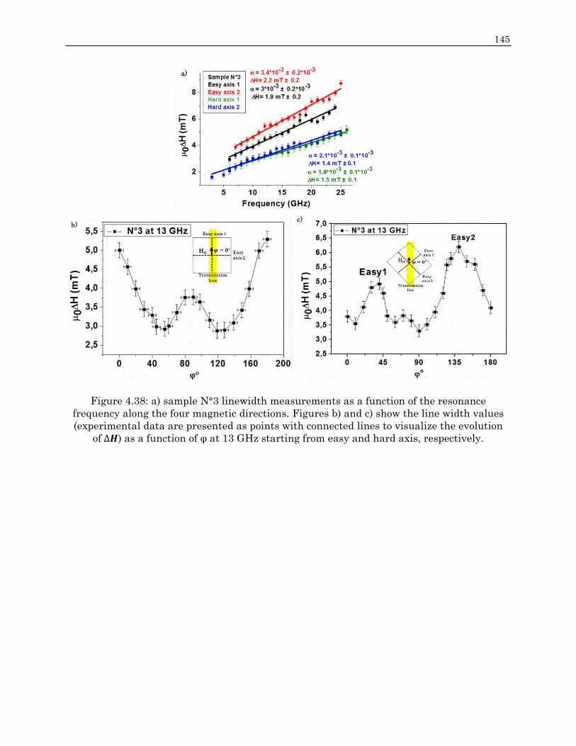
145
Figure 4.38: a) sample N°3 linewidth measurements as a function of the resonance
frequency along the four magnetic directions. Figures b) and c) show the line width values
(experimental data are presented as points with connected lines to visualize the evolution
of ∆𝑯) as a function of φ at 13 GHz starting from easy and hard axis, respectively.

146 Chapter 4: Structural and magnetic properties of “as deposited” CMS Heusler alloys
At the end of this section, a summary of the extracted relaxation parameters for the three
samples is given in the following table.
Sample Easy axis1 Easy axis 2 Hard axis 1 Hard axis 2
N°1
Phase L21
Phase B2
𝜶 = (2.1±𝟎. 𝟏)*10-3 ∆𝑯𝟎 = 𝟐. 𝟏 𝐦𝐓
−
𝜶 = (1.5±𝟎. 𝟑)*10-3 ∆𝑯𝟎 = 𝟑. 𝟏 𝐦𝐓
𝛼 = (3.2±0.1)*10-3 ∆𝐻0 = 4.1 mT
−
𝜶 = (2.6±𝟎. 𝟏)*10-3
∆𝑯𝟎 = 𝟏. 𝟔 𝐦𝐓
𝜶 =(1.6±𝟎. 𝟏)*10-3 ∆𝑯𝟎 = 𝟏. 𝟔 𝐦𝐓
𝛼 = (2.8±0.1)*10-3 ∆𝐻0 = 1.8 mT
N°2
𝜶 = (2.8±𝟎. 𝟏)*10-3
∆𝑯𝟎 = 𝟐. 𝟑 𝐦𝐓
𝜶 = (3. 𝟐 ± 𝟎. 𝟏)*10-3
∆𝑯𝟎 = 𝟏. 𝟗 𝐦𝐓
𝜶 = (3.5±𝟎. 𝟏)*10-3
∆𝑯𝟎 = 𝟏. 𝟑 𝐦𝐓
𝜶 = (2.3±𝟎. 𝟏)*10-3
∆𝑯𝟎 = 𝟐. 𝟒 𝐦𝐓
N°3
𝜶 = (3±𝟎. 𝟏)*10-3 ∆𝑯𝟎 = 𝟏. 𝟗 𝐦𝐓
𝜶 = (3.4±𝟎. 𝟏)*10-3 ∆𝑯𝟎 = 𝟐. 𝟐 𝐦𝐓
𝜶 = (1.9±𝟎. 𝟏)*10-3 ∆𝑯𝟎 = 𝟏. 𝟓 𝐦𝐓
𝜶 =(2.1±𝟎. 𝟏)*10-3 ∆𝑯𝟎 = 𝟏. 𝟒 𝐦𝐓
Table 4.7: damping factor 𝛂 and extrinsic line width ∆𝐇𝟎 values for both the two easy and
hard axes of the three samples N°1, N°2 and N°3.
4.3 Conclusion
In conclusion of this chapter, we demonstrated that our films present several
characteristics.
First, the sample N°1 and N°3 present two crystal orders. For the sample N°1 the two
phase corresponds to the L21 and B2 order phases, the first being majority. This is
confirmed by HAADF-STEM analysis which also shows a complete relaxation of our
sample by the presence of misfit dislocation at the interface between the CMS layer
and the MgO substrate. The L21 order has also been found to be the main phase in
sample N°3. However a second resonance peak observed in FMR let us think that a
minority B2 order is also present in this sample. Finally a small amount of Co-Si
exchange (4 to 6 %) is found for these two samples.
The situation of the sample N°2 is different. While the presence of L21 order has been
observed by X-ray, it is not the main phase in the material. Unfortunately we could
not perform structural analysis on this series of samples. However, the smaller
amplitude of the magnetization as compared to the other samples let us think that
Co/Mn and or Co/Si disorder is more important than for the two other samples.
MOKE measurements have shown small coercive fields of about 1 mT for the reference
samples of series N°1 and N°2. The switching process has been assumed to arise from
the propagation of either cross tie or 90° domain walls depending on the orientation of
the applied field with respect to the easy axis.
147
MOKE and FMR measurements have shown that all samples exhibit a cubic
anisotropy as expected, with an additional uniaxial anisotropy which can be aligned
either with an easy or a hard axis. The amplitude of the cubic anisotropy is few tens
of mT. These values are higher than the one reported in literature but in agreement
with our previous study [11 Ortiz]. The amplitude of the uniaxial anisotropy varies
from a few tenth to 2 mT. While the origin of this uniaxial anisotropy is still under
debate, we attribute it to the tetragonal distortion of the cell observed by X-ray
diffraction.
FMR measurements allowed extracting the static and dynamic magnetic parameters
of the samples. The magnetization, or magnetic moment, is found to be in good
agreement with the expected value of L21 or B2 order for samples N°1 and N°3. The
small discrepancies with respect to theoretical predictions are accounted to the
presence of Co/Si exchange.
The exchange constant value is in agreement with reported values except for sample
N°2, for which the disorder on Co sites is believed to be responsible of the decrease
magnetization and exchange values. Further investigation, for example via Brillouin
Light Scattering measurement, would be necessary to determine if it is really the
exchange value constant which is lower than other samples or if it is related to a
modification of the pinning constant due, for example, to surface effect.
The gyromagnetic ratio is found to be 28.7 GHz/T, leading to a g value of 2.05, showing
a small magnetic contribution from orbital moment.
FMR linewidth studies as a function of the frequency or angle φ has been carried out.
Based on other works, the values of the damping coefficient obtained in our samples
are believed to be upper limits to the intrinsic damping. This is due to inhomogeneity
contributions and 2 magnons scattering. The best value of the measured 𝛼 is 1.6*10-3,
which is to our knowledge close from the best values reported in CMS. In most cases
the best 𝛼 values are found in hard axis directions, unlike other work reported in
literature.
ΔH vs. fres and ΔH vs. φ measurements let us think for some anisotropic behavior of
the linewidth for all samples. However, experimental conditions, especially mixing
modes, leads to strong uncertainty of the measurement. Further analytical analysis,
especially taking into account the mosaicity of the sample and the two magnon
processes, is needed to conclude on this point and especially on an eventual anisotropy
of the damping coefficient.

148 Chapter 4: Structural and magnetic properties of “as deposited” CMS Heusler alloys
Chapter 4 References:
[1] G. Ortiz Hernandez, « Elaboration et étude des propriétés physiques de couches minces
monocristallines d’alliage de Heusler à faible amortissement magnétique pour
composants hyperfréquences », Université de Toulouse, Université Toulouse III-Paul
Sabatier, 2013.
[2] O. Gaier, « A study of exchange interaction, magnetic anisotropies, and ion beam induced
effects in thin films of Co2-based Heusler compounds », Ph. D. dissertation, Technical
University of Kaiserslautern, 2009.
[3] H. Pandey, P. C. Joshi, R. P. Pant, R. Prasad, S. Auluck, et R. C. Budhani, « Evolution of
ferromagnetic and spin-wave resonances with crystalline order in thin films of full-
Heusler alloy Co2MnSi », J. Appl. Phys., vol. 111, no 2, p. 023912, janv. 2012.
[4] M. Belmeguenai, F. Zighem, D. Faurie, H. Tuzcuoglu, S.-M. Chérif, P. Moch, K.
Westerholt, et W. Seiler, « Structural and magnetic properties of Co2MnSi thin films »,
Phys. Status Solidi A, vol. 209, no 7, p. 1328‑1333, juillet 2012.
[5] P. J. Webster, « Magnetic and chemical order in Heusler alloys containing cobalt and
manganese », J. Phys. Chem. Solids, vol. 32, no 6, p. 1221‑1231, 1971.
[6] V. Niculescu, K. Raj, T. J. Burch, et J. I. Budnick, « Correlation of the internal fields,
magnetic moments, and site preferences in Fe 3- x Mn x Si alloys », Phys. Rev. B, vol. 13,
no 7, p. 3167, 1976.
[7] Y. Takamura, R. Nakane, et S. Sugahara, « Quantitative analysis of atomic disorders in
full-Heusler Co[sub 2]FeSi alloy thin films using x-ray diffraction with Co Kα and Cu Kα
sources », J. Appl. Phys., vol. 107, no 9, p. 09B111, 2010.
[8] D. T. Cromer, « Compton Scattering Factors for Spherically Symmetric Free Atoms », J.
Chem. Phys., vol. 47, no 6, p. 1892, 1967.
[9] C. H. MacGillavry, G. D. Rieck, et International Union of Crystallography, International
tables for X-ray crystallography. Vol. 3, Vol. 3,. Birmingham: Published for the
International Union of Crystallography by the Kynoch Press, 1968.
[10] T. Mewes, « Separation of the first- and second-order contributions in magneto-optic
Kerr effect magnetometry of epitaxial FeMn/NiFe bilayers », J. Appl. Phys., vol. 95, no 10,
p. 5324, 2004.
[11] G. Ortiz, A. Garcia-Garcia, N. Biziere, F. Boust, J. F. Bobo, et E. Snoeck, « Growth,
structural, and magnetic characterization of epitaxial Co2MnSi films deposited on MgO
and Cr seed layers », J. Appl. Phys., vol. 113, no 4, p. 043921, 2013.
[12] L. McGuigan, R. C. Barklie, R. G. S. Sofin, S. K. Arora, et I. V. Shvets, « In-plane
magnetic anisotropies in Fe 3 O 4 films on vicinal MgO(100) », Phys. Rev. B, vol. 77, no 17,
mai 2008.
[13] J. Chen et J. L. Erskine, « Surface-step-induced magnetic anisotropy in thin epitaxial
Fe films on W(001) », Phys. Rev. Lett., vol. 68, no 8, p. 1212‑1215, février 1992.
[14] T. Leeb, M. Brockmann, F. Bensch, S. Miethaner, et G. Bayreuther, « In-plane
magnetic anisotropies in Fe films on vicinal Ag(001) and Au(001) surfaces », J. Appl.
Phys., vol. 85, no 8, p. 4964‑4966, avr. 1999.
[15] A. A. Baker, A. I. Figueroa, G. van der Laan, et T. Hesjedal, « Tailoring of magnetic
properties of ultrathin epitaxial Fe films by Dy doping », AIP Adv., vol. 5, no 7, p. 077117,
juill. 2015.
[16] M. Belmeguenai, H. Tuzcuoglu, M. S. Gabor, T. Petrisor, C. Tiusan, D. Berling, F.
Zighem, T. Chauveau, S. M. Chérif, et P. Moch, « Co2FeAl thin films grown on MgO
149
substrates: Correlation between static, dynamic, and structural properties », Phys. Rev.
B, vol. 87, no 18, p. 184431, mai 2013.
[17] H. Pandey, P. K. Rout, Anupam, P. C. Joshi, Z. Hossain, et R. C. Budhani,
« Magnetoelastic coupling induced magnetic anisotropy in Co2(Fe/Mn)Si thin films »,
Appl. Phys. Lett., vol. 104, no 2, p. 022402, janv. 2014.
[18] M. Belmeguenai, F. Zighem, T. Chauveau, D. Faurie, Y. Roussigne, S. M. Cherif, P.
Moch, K. Westerholt, et P. Monod, « Structural, static and dynamic magnetic properties
of Co2MnGe thin films on a sapphire a-plane substrate », J. Appl. Phys., vol. 108, no 6, p.
063926‑063926‑6, sept. 2010.
[19] P. E. Wigen, C. F. Kooi, M. R. Shanabarger, et T. D. Rossing, « Dynamic Pinning in
Thin-Film Spin-Wave Resonance », Phys. Rev. Lett., vol. 9, no 5, p. 206‑208, sept. 1962.
[20] R. Yilgin, Y. Sakuraba, M. Oogane, S. Mizukami, Y. Ando, et T. Miyazaki, « Anisotropic
intrinsic damping constant of epitaxial Co2MnSi Heusler alloy films », Jpn. J. Appl. Phys.,
vol. 46, no 3L, p. L205, 2007.
[21] O. Gaier, J. Hamrle, S. J. Hermsdoerfer, H. Schultheiß, B. Hillebrands, Y. Sakuraba,
M. Oogane, et Y. Ando, « Influence of the L21 ordering degree on the magnetic properties
of Co2MnSi Heusler films », J. Appl. Phys., vol. 103, no 10, p. 103910, mai 2008.
[22] B. Rameev, F. Yildiz, S. Kazan, B. Aktas, A. Gupta, L. R. Tagirov, D. Rata, D. Buergler,
P. Gruenberg, C. M. Schneider, S. Kämmerer, G. Reiss, et A. Hütten, « FMR
investigations of half-metallic ferromagnets », Phys. Status Solidi A, vol. 203, no 7, p.
1503‑1512, mai 2006.
[23] J. Hamrle, O. Gaier, S.-G. Min, B. Hillebrands, Y. Sakuraba, et Y. Ando,
« Determination of exchange constants of Heusler compounds by Brillouin light scattering
spectroscopy: application to Co2MnSi », J. Phys. Appl. Phys., vol. 42, no 8, p. 084005, avr.
2009.
[24] L. Ritchie, G. Xiao, Y. Ji, T. Y. Chen, C. L. Chien, M. Zhang, J. Chen, Z. Liu, G. Wu, et
X. X. Zhang, « Magnetic, structural, and transport properties of the Heusler alloys Co 2
MnSi and NiMnSb », Phys. Rev. B, vol. 68, no 10, sept. 2003.
[25] C. Liu, C. K. A. Mewes, M. Chshiev, T. Mewes, et W. H. Butler, « Origin of low Gilbert
damping in half metals », Appl. Phys. Lett., vol. 95, no 2, p. 022509, 2009.
[26] S.-Z. Qiao, J. Zhang, Y.-F. Qin, R.-R. Hao, H. Zhong, D.-P. Zhu, Y. Kang, S.-S. Kang,
S.-Y. Yu, G.-B. Han, S.-S. Yan, et L.-M. Mei, « Structural and Magnetic Properties of Co 2
MnSi Thin Film with a Low Damping Constant », Chin. Phys. Lett., vol. 32, no 5, p. 057601,
mai 2015.
[27] S. Andrieu, A. Neggache, T. Hauet, T. Devolder, A. Hallal, M. Chshiev, A. M. Bataille,
P. Le Fèvre, et F. Bertran, « Direct evidence for minority spin gap in the Co2MnSi Heusler
alloy », Phys. Rev. B, vol. 93, no 9, p. 094417, mars 2016

150 Chapter 5: Effect of He+ ions irradiation on structural & magnetic properties of CMS
Chapter 5: Effect of He+ ions
irradiation on structural and
magnetic properties of CMS
Heusler alloys
In this chapter we investigate the effect of He+ ion irradiation on structural and magnetic
properties of the three studied CMS samples presented in chapter 4 as follows:
- Samples of series N°1: the same substrate has been cut in 4 equivalent pieces of 5 x
5 mm². One is the reference sample presented in chapter IV and the three others have
been irradiated at fluences of 1*1015, 5*1015 and 1*1016 ions/cm². The structural
properties of this series of samples have been studied by X-ray diffraction for the four
samples and by HAADF-STEM for the reference and 1*1016 irradiated samples. The
magnetic properties have been studied by MOKE for the reference and 1*1016
irradiated samples and by FMR and PPMS magnetometry for the four samples.
- Sample of series N°2: this series of samples have been cut into 6 pieces of 3 x 3 mm².
One piece is the reference sample presented in chapter IV. The irradiation doses for
the other samples are 1*1014, 1*1015, 4*1015, 1.2*1016 and 1*1017 ions/cm². X-ray
diffraction 𝜑 scan measurement was only performed on the reference sample to check
the existence of L21 phase, even with a weak signal, by CEMES Co source
diffractometer (Figure 4.9). Thus, we were not able to conduct a quantitative study of
the atomic disorder on this series. The magnetic properties have been studied by
MOKE for the reference sample and by FMR for all samples.
- Sample of series N°3: This series of samples have been cut into 5 pieces of 3 x 3 mm².
One piece is the reference sample presented in chapter IV. The irradiation doses for
the other samples are 1*1014, 1*1015, 1*1016 and 1*1017 ions/cm². X-ray diffraction
measurements with Cu source has been performed on the reference, 1*1016 and 1*1017
irradiated samples. HAADF-STEM analysis have been performed on the reference and
1*1017 irradiated samples. The magnetic properties have been studied only by FMR
for all the samples.
The different results obtained for the reference samples of the three series have been
presented in the previous chapter. In this chapter we will begin with the simulations of the
effect of irradiation with He+ ions on the structural disorder of the CMS. Then we will present

151
the structural analysis performed by X-ray diffraction and HAADF-STEM on series N°1 and
N°3. The last part of this chapter will focus on the evolution of the magnetic parameters
induced by the irradiation, with respect to the structural modifications.
5.1 Irradiation with Helium ions (He+) at 150 keV
In the present thesis, the species used for ion irradiation is helium ions. The main goal of
using light ions, such as He+, was to investigate how the introduction of a controlled disorder
is possible to promote the advent of partially disordered phases. Moreover, the high kinetic
energy is chosen to first avoid He+ implantation in the CMS layer and also to minimize local
defects at low doses. Indeed, ion irradiation can be considered in a very simplified approach
to act as an annealing process for low doses which can lead to structural improvement. He+
ions irradiation has been used in previous work done by [1-3 Fassbender] to modify the
magnetic properties of Pt-Co system, resulting from ion-induced interfacial mixing. Also, an
enhancement of chemical ordering and long-range order L10 in FePt and FePd thin films by
130 KeV He+ irradiation was reported by Ravelosona et al.[4,5 Ravelosona]. Based on the
mentioned magnetic and structural properties presented in the previous chapter, Ion
irradiation of high energy (150 KeV) of different fluences doses range from 1014 to 1017
ions/cm2 will impact our CMS thin films
In our experiments we focused our work on a Co2MnSi layer with a thickness of 42 and
50 nm. Prior to the experiment, the irradiation process was simulated using either the well-
known SRIM software (Stopping and Range of Ions in Matter) or a homemade IPROS code
[6-8]. These softwares are based on Monte-Carlo binary collision process. From the output
results, it is then possible to estimate the Helium range and the concentration distribution of
displaced atoms in the ternary layer.
The starting point of the calculation was to reduce as much as possible the presence of helium
atoms in the Heusler layer and for this reason an energy of 150 keV was chosen. In the
following section the results of the simulation will be analyzed.
5.1.1 Simulation of Co2MnSi irradiation with He+ ions
Prior to ion irradiation, the appropriate parameters to predict the helium distribution
as well as the damage impact of the bombardment on the structural properties of the Heusler
layer were carried out. For this purpose, simulations of the irradiation process were
performed using Monte-Carlo binary collision softwares [6-8].
In the case of He+ irradiation of Co2MnSi two criteria must be fulfilled: (i) a low
concentration of helium atoms in the active layer and (ii) a low defect density induced by ion
bombardment. These are the major conditions to ensure a suitable improvement of the
structural and magnetic properties of the Heusler layer, at least for low fluences. To perform
this work an atomic density of 8.85x10²² atoms/cm3 for the Heusler film was used and about
300000 incoming He ions with an energy of 150 keV were launched.
Figure 5.1 shows the simulated Helium concentration profile as a function of depth for
a fluence of 1x10¹⁴ ions/cm-2. Let’s keep in mind that the CMS layer of 42 or 50 nm thickness

152 Chapter 5: Effect of He+ ions irradiation on structural & magnetic properties of CMS
is deposited on MgO substrate and covered by a capping layer of MgO (10 nm) to prevent
oxidation. The simulation was performed for the CMS monolayer of stoichiometric
composition (50% Co, 25% Mn and 25 % Si atoms). From figure 5.1, we have deduced the
projected range Rp=486 nm of helium in CMS layer. The profile clearly shows that the peak
of the implantation concentration is located in the MgO substrate and that the depth at which
most of the ions stopped in the sample is far below the CMS layer. In figure 5.2 the He ion
concentration was plotted in log scale for 3 increasing fluences. The figure shows that in the
CMS region the concentration of He is about 0.1% of the peak value and may be considered
as negligible.
Figure 5.1: Helium concentration as a function of depth.
Figure 5.2: distribution of different concentration doses of He+ ions at 150 KeV as a
function of CMS layer depth.
In order to estimate the number of defects created along the helium ion trajectory, we plotted
in figure 5.3 the vacancy concentration of each element of the CMS film as a function of depth.
The total damage introduced into the crystal lattice at a particular fluence of 1x10¹⁴ ions/cm2
can be estimated taking into account that most displacements resulted in creation of Frenkel
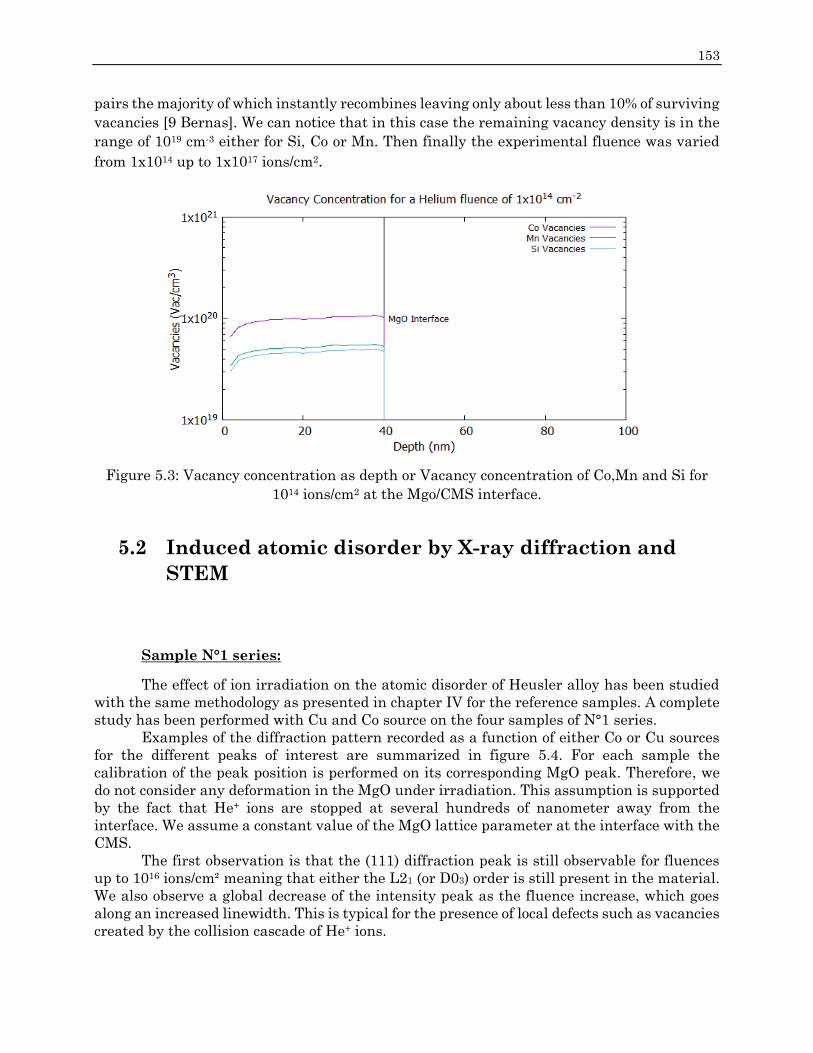
153
pairs the majority of which instantly recombines leaving only about less than 10% of surviving
vacancies [9 Bernas]. We can notice that in this case the remaining vacancy density is in the
range of 1019 cm-3 either for Si, Co or Mn. Then finally the experimental fluence was varied
from 1x10¹⁴ up to 1x10¹⁷ ions/cm2.
Figure 5.3: Vacancy concentration as depth or Vacancy concentration of Co,Mn and Si for
1014 ions/cm2 at the Mgo/CMS interface.
5.2 Induced atomic disorder by X-ray diffraction and
STEM
Sample N°1 series:
The effect of ion irradiation on the atomic disorder of Heusler alloy has been studied
with the same methodology as presented in chapter IV for the reference samples. A complete
study has been performed with Cu and Co source on the four samples of N°1 series.
Examples of the diffraction pattern recorded as a function of either Co or Cu sources
for the different peaks of interest are summarized in figure 5.4. For each sample the
calibration of the peak position is performed on its corresponding MgO peak. Therefore, we
do not consider any deformation in the MgO under irradiation. This assumption is supported
by the fact that He+ ions are stopped at several hundreds of nanometer away from the
interface. We assume a constant value of the MgO lattice parameter at the interface with the
CMS.
The first observation is that the (111) diffraction peak is still observable for fluences
up to 1016 ions/cm² meaning that either the L21 (or D03) order is still present in the material.
We also observe a global decrease of the intensity peak as the fluence increase, which goes
along an increased linewidth. This is typical for the presence of local defects such as vacancies
created by the collision cascade of He+ ions.

154 Chapter 5: Effect of He+ ions irradiation on structural & magnetic properties of CMS
Figure 5.4: X-ray diffraction 2𝜽 scan for reference and 3 irradiated samples of N°1 for Co
and Cu diffractometer sources. a), b) and c) represents the 111,002 and 022 peaks acquired
by Co source. d) and e) presents the 002 and 004 peaks acquired by Cu source.
Interestingly, we also observe with both sources a shift in the (002) diffraction peak
towards low angles compared to the reference sample peak position, indicating an increase of
the out-of-plane lattice parameter of CMS with the increase of ion fluence. With the Co source,
we also observe a shift in the (022) diffraction peak while the (111) peak is kept almost at the
same Bragg angle (from 31.86° to 31.83°). Calculating the lattice parameters (table 5.1) from
the 2𝜽 Bragg angle of the three peaks with the Co source, we find that only the out-of-plane
lattice parameter c varies from 5.67 Ǻ for the reference sample to 5.69 Ǻ for the 5.1015 and
1016 ions/cm² irradiated sample, while the in-plane parameter is kept constant and equals to
5.63 Ǻ. Same values of the c parameters are obtained from the diffraction peaks with the Cu
source. Then the most obvious conclusion of this observation is that the irradiation induces a
tetragonal distortion of the cell but then the volume of the cell is not kept constant with
respect to the reference sample.
GPA analysis performed on HAADF-STEM images obtained from the sample
irradiated at 1016 ions/cm² have shown similar values of strain deformation as for the
reference sample. An example of strain calculation is shown in Figure 5.5. As for the sample
reference, we found the out of plane strain of the order of 34 ± 1.5% with respect to the MgO,
and no particular additional strain effect is observed as compared to the reference sample.
This is not surprising. Indeed, the strain in the CMS layer is calculated with respect to the
MgO. The difference of out-of-plane lattice parameter measured by X-ray for the CMS would
lead theoretically to a change in the strain with respect to the MgO from 𝜺𝒛𝒛 = 34.6% to 35%,
so the variation is below the uncertainty of the GPA analysis. For the in plane deformation,
which is supposed to be constant according to the X-ray diffraction, we found an average value

155
for the irradiated sample of 𝜺𝒙𝒙 = -5.1 ± 0.4 %. This is slightly higher than for the reference
sample. This could be due to an eventual modification of the MgO parameters under
irradiation. However the observed difference between the reference sample and the irradiated
one is also of the order of the experimental uncertainty. Then, we believe that GPA analysis
is not sensitive enough to detect such small variations of strain induced by the ion irradiation
as the experimental uncertainty is of the order of the expected variation.
Figure 5.5: GPA analysis performed on sample N°1 irradiated at 1016 ions/cm2 shows the in-
plane and out-of-plane deformation of -5.1 ±0.4 and 34.1 ±1.5, respectively.
REF (Å) 1015 (Å) 5*1015 (Å) 1*1016 (Å)
a 5.63 5.63 5.63 5.63
c 5.67 5.68 5.69 5.69
Table 5.1: lattice parameter of sample N°1 reference and irradiated ones as a function of the
ion fluence.
In order to determine the different disorder parameters for the four series of sample
N°1, the same methodology presented in chapter IV is used for the reference sample. The
results for the deduced 𝛼, 𝛽 and 𝛾 are presented in figure 5.6. For all samples, we observe that
the 𝛽 parameter, i.e. Co/Si disorder, remains almost constant (0.04 ± 0.02) whatever the ion
fluence is used. Additionally 𝛼 increases from 0.14 ± 0.01 to 0.22 ± 0.01 for the reference
sample and the 1016 irradiated one, respectively. There is a clear step at 5*1015 for 𝛼. Similarly
the 𝛾 parameter, i.e. Co/Mn disorder, increases significantly for fluences above 5*1015. For
lower fluences, the Co-Mn substitution (𝛾) is not detectable within the uncertainty of the
measurements, meaning it is less than 0.02.

156 Chapter 5: Effect of He+ ions irradiation on structural & magnetic properties of CMS
Figure 5.6: 𝜶,𝜷 𝒂𝒏𝒅 𝜸 atomic disorder percentage of sample N°1 series as a function of the
irradiated fluences used.
In order to state about the organization of the induced atomic disorder observed by X-
Ray diffraction, HAADF-STEM has been performed on the sample irradiated at 1016 ions/cm².
While the B2 order in the reference sample is only observed in small regions of similar
size as the black box in Figure 4.13-a in chapter IV, it can be observed in more extended areas
for a fluence of 1016 ions/cm². This is shown in Figure 5.7-a. The B2 order can be observed
either from the intensity profile presented in Figure 5.7-b corresponding to the lines in figure
5.7-a or statistically over the selected area (black box in figure 5.7-a as shown in figure 5.7-c).
Similar values for the STEM intensity of the Mn and Si columns are measured while the
intensity corresponding to the Co columns remains higher2. On other part of the sample we
still observe the L21 order (Figure 5.7-d). Based on this result and in addition to the observed
increase of the 𝛼 parameter, we suggest that ion irradiation induces a L21 to B2
transformation in this sample. Moreover we suggest that the transformation occurs around
the initial B2 grains.
Dealing with the increase Co-Mn exchange, we already mentioned that HAADF-STEM
is not sensitive to this atomic exchange as the Z numbers of both atoms are very close.
Therefore, it is difficult to state about either D03 grains grow in the initial matrix or if this
atomic exchange occurs as punctual defects in the entire alloy, including in the B2 phase. This
issue can be addressed via magnetization amplitude measurements with PPMS. Indeed we
show in Figure 5.12 that the decrease of the magnetization observed for the alloy is in
agreement with a model in which we consider a B2 order with magnetization 1.25 T and a
L21’3 phase with decreasing magnetization. With this model, the calculation of the average
magnetization is done considering a volume of the B2 phase proportional to α/0.5 (𝛼 = 0.5
corresponding to a full B2 order) and a L21’ phase proportional to 1-𝛼/0.5. The result of the
calculation for the magnetization of this L21’ phase is presented in table 5.2. The obtained
2 Note here that the denotation Mn and Si does not have a real signification as we are not able to
distinguish the two elements. Then we arbitrarily set the first atomic column in blue to be the Mn and
the red to be the Si in figure 5.7-a. We did the same denotation in figure 5.9-a. 3 The denotation L21’ is proposed in order to remind that the initial L21 phase has been submitted to
atomic disorder and does not correspond anymore to a “pure” L21 order.
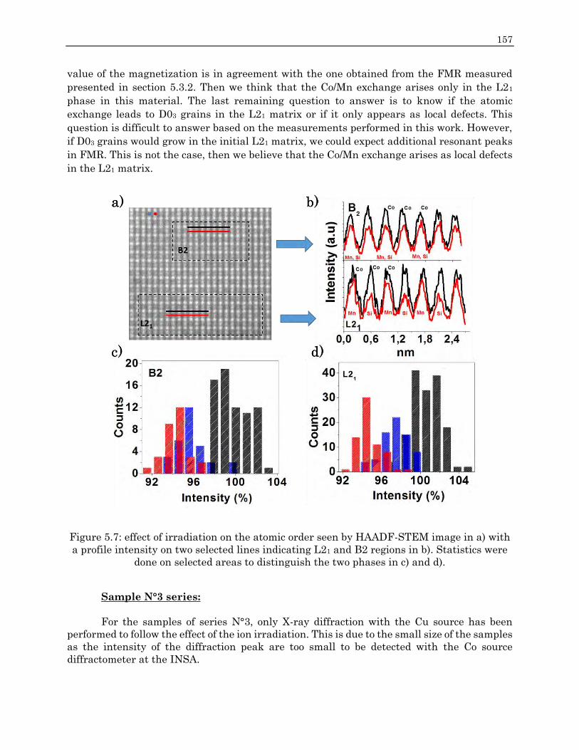
157
value of the magnetization is in agreement with the one obtained from the FMR measured
presented in section 5.3.2. Then we think that the Co/Mn exchange arises only in the L21
phase in this material. The last remaining question to answer is to know if the atomic
exchange leads to D03 grains in the L21 matrix or if it only appears as local defects. This
question is difficult to answer based on the measurements performed in this work. However,
if D03 grains would grow in the initial L21 matrix, we could expect additional resonant peaks
in FMR. This is not the case, then we believe that the Co/Mn exchange arises as local defects
in the L21 matrix.
Figure 5.7: effect of irradiation on the atomic order seen by HAADF-STEM image in a) with
a profile intensity on two selected lines indicating L21 and B2 regions in b). Statistics were
done on selected areas to distinguish the two phases in c) and d).
Sample N°3 series:
For the samples of series N°3, only X-ray diffraction with the Cu source has been
performed to follow the effect of the ion irradiation. This is due to the small size of the samples
as the intensity of the diffraction peak are too small to be detected with the Co source
diffractometer at the INSA.

158 Chapter 5: Effect of He+ ions irradiation on structural & magnetic properties of CMS
The evolution of the (002) and (004) peaks for samples irradiated at 1016 and 1017
ions/cm² are shown in figure 5.8. Similarly to sample N°1, we observe an increase of the out
of plane deformation but it is found to be more important than for the samples N°1. Indeed
the out of plane lattice parameter is found to be 5.70, 5.72 and 5.73 Ǻ for the reference, 1016
and 1017 ions/cm² irradiated samples respectively. These values are very important as
compared to the expected one and bigger than for sample N°1. Unfortunately no GPA analysis
could be performed on these samples as the MgO zone is not observable on the HAADF-STEM
images. Then we could not study the eventual deformation of the CMS with respect to the
substrate.
Figure 5.8: Evolution of 002 and 004 diffraction peaks as a function of irradiation fluence for
the reference, irradiated at 1016 and 1017 ions/cm2 of N°3 series samples performed by Cu
source diffractometer.
As the measurements were done with the Cu source, we can calculate the evolution of
the Co/Si exchange. The 𝛽 parameter is found to vary from 0.06 to 0.15 and 0.22 for the
irradiated sample at 1016 and 1017 ions/cm², respectively. Comparing the samples irradiated
at 1016 for series N°1 and N°3, we observe a clear difference in the evolution of 𝛽 disorder
parameter. While it was found to be roughly constant for the N°1 series, it increases by more
than a factor 2 for the N°3 series at 1016 ions/cm².
This behavior is surprising and one of the most important conclusions we can state is that the
different samples do not show the same behavior under irradiation. This is a potential
problem for the reproducibility of the method and implies a full study of the structural order
for each sample to understand their magnetic properties.
HAADF-STEM has been performed on the sample irradiated at 1017 ions/cm² for N°3
series. An example of HAADF-STEM image is shown for the [110] direction of CMS in Figure
5.9. The statistics of the maximum amplitude of each atomic column performed on a zone of
20 x 22 atomic columns are shown in figures 5.9-e and 5.9-f. We clearly see that the Mn and
Si intensities are very similar and below the intensity of Co. This is similar to what we
observed for sample N°1. However, the main difference with the sample irradiated at 1016
ions/cm² of the N°1 series is that here we do not observe variations from one zone of the sample
to another. This sample looks quite homogeneous with only punctual variations of local
intensities in the Mn/Si amplitude that could reflect some remaining L21 order as shown by
the blue circles in figure 5.9-c. HAADF-STEM performed in the [100] direction presented in

159
figure 5.9-b, confirms that the Mn/Si columns have lower intensities than the Co columns
(figure 5.9-d).
At first sight, this sample can then be concluded to be almost completely in the B2
order. However this result is not in agreement neither with the value of 𝛽 determined by X-
ray nor by the FMR measurements presented in section 5.3.2, for which two crystal orders
are well separated at 1017 ions/cm2. First, the 𝛽 value is close from the expected value for a
pure A2 crystal order (𝛼, 𝛽 and 𝛾 are equal to ½, ¼ and ¼, respectively for A2) but this phase
would be revealed in HAADF-STEM by having the same STEM intensities for all atomic
columns, including the Co ones, due to the random distribution of the atoms on the different
atomic sites. This is clearly not observed in our experiment for which the Co intensity is
always above the one of the Si or Mn columns. Then we do not think that the A2 order is
present.
Figure 5.9: HAADF-STEM has been performed on the sample irradiated at 1017 ions/cm² for
the series N°3 along [110] and [100] CMS directions in a) and b) respectively. Intensity
profiles in c) show some remaining L21 regions in blue circles while in d) Mn and Si are
indistinguishable. Statistics in e) and f) show that Co has higher intensities than Mn and Si.

160 Chapter 5: Effect of He+ ions irradiation on structural & magnetic properties of CMS
Based on the evolution of the disorder parameters observed in the samples of series
N°1, we propose the following scenario, sketched on figure 5.10. We believe that starting from
a L21 order, the effect of irradiation is to induce 2 kinds of transformation. The first one is a
L21-B2 transition as shown for sample N°1 and in agreement with the STEM profile in sample
N°3 and FMR measurements presented below. The second transformation concerns only the
remaining L21 phase for which we believe that Co/Mn exchange first occurs, similarly to
sample N°1. Then, above a threshold fluence, Co-Si exchange takes place for the Co atoms
being on the Mn sites. In this manner, Co atoms can be found on Si sites, leading to a high 𝛽
value, but Si atoms are not on Co sites, explaining the remaining high intensity of Co columns
in STEM. Indeed as Co and Mn gives the same STEM intensities (as a first approximation),
this double exchange scenario would lead to high intensity on Co/Mn columns and lower
intensities in randomly distributed Mn/Si/Co columns and this phase would not be very
different in HAADF-STEM image from a B2 order. This phase could be considered as a mix
of D03 and B2 phase, but not to the A2 order as no Si would be found on Co sites. Let’s note
that this scenario does not avoid Co/Si exchange also in the B2 order, which most probably
occurs at very high fluence.
If this double exchange scenario is right, it also means that our model for the
calculation of the disorder parameters is incorrect, at least for fluence of 1017. Indeed, this
model implicitly considers the symmetric exchange of the atoms positions. This would not be
the case for double exchange. A complete model for calculating the atomic disorder
parameters would need a set of individual rate of presence of each chemical entity on each
atomic site. Also the presence of local defects should be taken into account in the model to
consider the decrease of the peak amplitude. However, this approach leads to too many
unknown parameters and is not realistic. Then the model used in this work has most probably
to be limited to low irradiation fluence.
Figure 5.10: proposed scenario of the irradiation effect on CMS samples starting from L21
phase to D03 (Co-Mn disorder) and then a B’2 (Co-Si disorder) phase.
Several conclusions can be stated from the structural analysis of the
irradiated sample. First, out of plane deformation is induced by the He+
irradiation. In addition, local defects in the alloy appear for ions fluence above 1016
ions/cm².
The mechanical distortion is accompanied by a modification of the local
atomic arrangement as demonstrated by the evolution of the disorder parameters
for the sample of series N°1. Based on this series of sample we believe that, for low
ion fluence, the B2 order is favored with respect to the L21 order, especially if the
B2 order is already present. Additionally, we believe that above a threshold fluence,
most probably around 5*1015 or 1016 ions/cm², Co/Mn swap occurs due to the low

161
energy formation of this kind of defects. Then ion irradiation seems to be
inappropriate for improving the L21 order in Co2MnSi, as it nucleates most
probably some local defects of D03 type. However ion irradiation is confirmed to
improve the B2 order, as observed by Gaier et al. However neither HAADF-STEM
nor X-ray diffraction allows to state about the presence of Co/Mn swap in the
created B2 phase.
For higher fluences, the partial results obtained from X-ray diffraction and
HAADF-STEM imaging performed on the samples of the series N°3 let us think that
a potential double exchange arises in the L21/D03 order. Indeed, the only possibility
to explain the contrast in STEM is to consider that no (or only few) Si atoms get to
the position of Co atoms. Moreover, the presence of Co atoms on Si sites is coherent
with both the STEM contrast and the high value of the β parameter. This
assumption can be partially supported by the calculated energy formation of Co
antisite realized by Piccozzi et al [10 Picozzi]. They have found relatively low value
of 0.8 eV which, corroborated to the presence of local defects in the matrix, allow
for the displacement of Co atoms far from their original site.
Let us now focus on the effect of ion irradiation on the magnetic properties of the alloy.
We will first show how the basic properties of the magnetic material, such as the average
magnetization amplitude and coercive fields are affected. Then we will present dynamic
measurement which will allow studying more in details the effect of irradiation on local
anisotropies and on the evolution of magnetic parameters for the different crystal order as a
function of the ion fluence. Finally the last part of this chapter will be devoted to the
presentation of preliminary results on the effect of ion irradiation on the dynamic relaxation.
5.3 Modifications of magnetic properties by He+ ions
irradiation
To study the effect of the ion irradiation on the coercive field and magnetization
amplitude, MOKE has been performed on the sample of the series N°1 irradiated at 1016
ions/cm² while PPMS measurements have been performed on the four samples of the series.
The results of these experiments are presented in the next subsection.
5.3.1 Static magnetic properties
Basically, similar features as for the reference samples are recovered. However, few
differences can be observed. The most obvious observation concerns the amplitude of the
coercive field 𝜇0Hc. While similar values of 𝜇0Hc were observed for the reference sample as a
function of the angle 𝛼 between the direction of the applied field and the easy axis, the
irradiated sample shows a clear difference between the easy and hard directions as can be
seen in Figure 5.11-a. This reflects an increase of the crystal anisotropy, in agreement with
the values of the saturation field presented in Figure 5.11-b. This will also be confirmed by
FMR measurements.
The increase of the coercive fields is typical in switching mechanisms dominated by
the propagation field. Indeed, point defects are generally assumed to decrease the nucleation
field of magnetic domains via a reduction of the local energy landscape. However, point defects
acts as a friction term in the dissipative process during the propagation of the domains.

162 Chapter 5: Effect of He+ ions irradiation on structural & magnetic properties of CMS
Therefore, an increase of the coercive fields can be accounted for an increase of the
propagation field. This is due to the fact that the domain wall widths, being of a few tens of
nanometer for Neel walls, average the effect of local defects over large distance. The friction
arises from local distortion of the domain around point defects. A complete review of these
processes can be found in the book “Magnetic Domains” by Hubert and Schäfer [12 Hubert &
Schäfer].
Figure 5.11: Coercive field (a) and saturation field (b) as a function of the applied field
direction with respect to the easy axis, where the black and red curves correspond
respectively to the reference sample of series N°1 and irradiated one at 1016 ions/cm2. C)
Example of LMOKE signal after symmetry process, showing the different switching
mechanisms in the different directions.
Additionally to the anisotropic behavior of the coercive fields, we also observe that the
two easy axes and the two hard axes do not show similar magnetic switching mechanisms.
This is shown in figure 5.11-c. As the four axes behave differently, one can think that some
uniaxial anisotropy tilted with respect to the easy axis appears. FMR measurements
presented in the next sub-section will show that no uniaxial anisotropy is present at 1016
ions/cm2. Then the origin of these differences between the 4 axes is not clear. However, as
demonstrated by the structural analysis and further by FMR measurements, this sample
shows clearly two different phases with different magnetic parameters (𝜇0Ms, 𝜇0Hk). Then,
as MOKE measures the average magnetic properties of the sample, it is extremely difficult to
distinct the magnetic behavior of an individual phase and we believe that the observed
differences are accounted for the different behavior of the two phases.
PPMS magnetometry measurements have also been performed on the four samples of
N°1series. The result of the calculated magnetization amplitude is shown in figure 5.12. We
clearly observe a decrease of magnetization with an ion fluence above 1015 ions/cm². The
uncertainty of the magnetization is due to the uncertainty on the exact dimensions of each

163
sample measured with a precision of a few microns. Magnetization values are reported in
table 5.2. Considering that the samples are made up of the B2 crystal order with a
magnetization of 1.25 T and a second phase with varying magnetization amplitude due to D03
type disorder, we can evaluate the magnetization of the second phase by considering the
volume ratio of each phase. As explained in section 5.2, the volume of the B2 phase is
calculated with respect to the full B2 order as 𝛼/0.5. The values of 𝛼 are given in figure 5.6.
The volume of the second phase is then 1- 𝛼/0.5. Magnetization values of the second phase are
presented in table 5.2. We will see that FMR measurements are in good agreement with this
approach and then support our initial assumption of two distinct crystal orders, one being the
B2 order with constant magnetization and the second one having a decreasing magnetization.
Figure 5.12: PPMS average magnetization measurements for the four samples of N°1 series.
N°1 sample at
different
Fluences
(ions/cm²)
µ0Ms (T)
measured
Proportion of
B2 phase (1.25
T)
(α/0.5)
Proportion of
second phase
(1 - α/0.5)
µ0Ms second
phase (T)
REF 1.25 ± 0.02 0.28 0.72 1.25± 0.02
1015 1.25 ± 0.02 0.26 0.74 1.25± 0.02
5*1015 1.2 ±0.02 0.4 0.6 1.16± 0.02
1016 1.16 ± 0.02 0.41 0.59 1.1± 0.02
Table 5.2: magnetization values of N°1 series for both phases.
5.3.2 FMR measurements of irradiated samples: effect of
irradiation on magnetic parameters
Sample N°1 series:
FMR measurements have been performed on the four samples of N°1 series to extract
the magnetic parameters of each crystal phase as a function of the ion fluence. Examples of
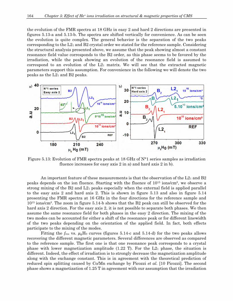
164 Chapter 5: Effect of He+ ions irradiation on structural & magnetic properties of CMS
the evolution of the FMR spectra at 18 GHz in easy 2 and hard 2 directions are presented in
figures 5.13-a and 5.13-b. The spectra are shifted vertically for convenience. As can be seen
the evolution is quite complex. The general behavior is the separation of the two peaks
corresponding to the L21 and B2 crystal order we stated for the reference sample. Considering
the structural analysis presented above, we assume that the peak showing almost a constant
resonance field value corresponds to the B2 order, as this phase seems to be favored by the
irradiation, while the peak showing an evolution of the resonance field is assumed to
correspond to an evolution of the L21 matrix. We will see that the extracted magnetic
parameters support this assumption. For convenience in the following we will denote the two
peaks as the L21 and B2 peaks.
Figure 5.13: Evolution of FMR spectra peaks at 18 GHz of N°1 series samples as irradiation
fluence increases for easy axis 2 in a) and hard axis 2 in b).
An important feature of these measurements is that the observation of the L21 and B2
peaks depends on the ion fluence. Starting with the fluence of 1015 ions/cm², we observe a
strong mixing of the B2 and L21 peaks especially when the external field is applied parallel
to the easy axis 2 and hard axis 2. This is shown in figure 5.13 and also in figure 5.14
presenting the FMR spectra at 16 GHz in the four directions for the reference sample and
1015 ions/cm². The zoom in figure 5.14-b shows that the B2 peak can still be observed for the
hard axis 2 direction. For the easy axis 2, it is not possible to separate both phases. We then
assume the same resonance field for both phases in the easy 2 direction. The mixing of the
two modes can be accounted for either a shift of the resonance peak or for different linewidth
of the two peaks depending on the orientation of the applied field. In fact, both effects
participate to the mixing of the modes.
Fitting the fres vs. 𝜇0H0 curves (figures 5.14-c and 5.14-d) for the two peaks allows
recovering the different magnetic parameters. Several differences are observed as compared
to the reference sample. The first one is that one resonance peak corresponds to a crystal
phase with lower magnetization amplitude (1.22 T). For the L21 phase, the situation is
different. Indeed, the effect of irradiation is to strongly decrease the magnetization amplitude
along with the exchange constant. This is in agreement with the theoretical prediction of
reduced spin splitting caused by Co/Mn exchange by Picozzi et al. [10 Picozzi]. The second
phase shows a magnetization of 1.25 T in agreement with our assumption that the irradiation

165
favors the B2 order in the alloy. Concerning the cubic anisotropy amplitude, both phases show
similar values compared to the reference sample.
The main difference with the reference sample is the appearance of a uniaxial
anisotropy aligned at about 23° from easy axis 2. This effect is most probably related to the
tetragonal deformation observed by X-ray diffraction. We remind that MOKE measurements
for the reference sample made us think that a small uniaxial anisotropy was aligned with one
easy axis. Then we think that the tetragonal distortion allows for the rotation of the
anisotropy direction in the plane of the layer. However, we do not know if this effect can be
caused by an eventual interface effect with the MgO as we made the assumption that the
MgO lattice parameter is not influenced by the irradiation.
Figure 5.14: a) and b) presents the four easy and hard directions FMR spectra at 16 GHz of
N°1 reference and irradiated at 1015 ions/cm2.In c) and d) 𝒇𝒓𝒆𝒔vs. 𝝁𝟎H0 curves for both
phases of N°1 irradiated at 1015 ions/cm2.
Similar treatment is applied for fluences of 5*1015 and 1016 ions/cm². At 5*1015 fluence,
we now observe that the position of the peaks for the L21 and B2 phases respectively are
superposed for the two easy axes while a shift is observed for the two hard axes (figure 5.15-
a). This means that the uniaxial anisotropy is now superposed to a hard axis (hard axis 2 in
our case) direction. At 1016 fluence, the effect of the uniaxial anisotropy has disappeared as
the position of both L21 and B2 peaks superpose for the two easy and the two hard axes (figure
5.15-b). While the tetragonal distortion was found to increase between 1*1015 and 5*1015

166 Chapter 5: Effect of He+ ions irradiation on structural & magnetic properties of CMS
ions/cm², which could explain the increased amplitude (see table 5.3) and rotation of the
uniaxial anisotropy, the fact that the uniaxial anisotropy disappears at 1016 while the out-of-
plane parameter is the same means that the internal strain have been relaxed. Then we
believe that the amplitude of the uniaxial anisotropy is most probably related with the
internal mechanical strain, the relaxation of the latter being mediated by the increased
number of vacancies by the irradiation.
Figure 5.15: FMR absorption spectra obtained for the four easy and hard axes directions for
a) N°1 irradiated at 5*1015 and b) N°1 irradiated for 1016 ions/cm2 fluence.
Figure 5.16 presents the evolution of the fres vs 𝜇0H0 for all fluences of N°1 series for
each crystal order. For convenience and clarity, only one easy and one hard axis for each
fluence is presented. The deduced magnetic parameters obtained from these curves are
summarized in table 5.3. Despite the increasing uniaxial anisotropy, the B2 crystal order
shows similar magnetic parameters whatever the ion fluence.
Additionally, we observe an increase of the cubic anisotropy and of the gyromagnetic
ratio. The latter shows that the orbital moment increases with disorder. The study of the
linewidth presented in the next subsection will show that the spin-orbit coefficient λSO is
roughly constant as a function of the dose. Then the increased orbital moment seems to be
the origin of the increased anisotropy and decreased g value.
Figure 5.16: Evolution of the 𝒇𝒓𝒆𝒔vs. 𝝁𝟎H0 curves for both phases of N°1 series. In a) shows
the L21 phase evolution as irradiation dose increases while in b) all curves have the same
behavior and are identified for the B2 phase.

167
N°1 series
(ions/cm2)
Ref Irr. at 1015 Irr. at 5*1015 Irr. at 1016
µ0Ms1 (T) 1.26± 0.02 1.22± 0.02 1.14± 0.02 1.1± 0.02
µ0Ms2 (T) 1.25± 0.02 1.25± 0.02 1.25± 0.02 1.25± 0.02
µ0Hk1 (mT) 36± 0.2 34± 0.2 42± 0.2 45± 0.2
µ0Hk2 (mT) 𝟑𝟐 ± 𝟎. 𝟐 33± 0.2 35± 0.2 36± 0.2
𝜸1 (GHz/T) 28.7± 0.1 28.7± 0.1 28.8± 0.1 28.9± 0.5
𝜸2 (GHz/T) 28.7± 0.1 28.7± 0.1 28.7± 0.1 28.7± 0.3
φu
(deg)
0 23 ± 2 45 ± 2 0
µ0Hu
(mT)
< 1 1 ± 0.2 1.9 ± 0.1 0
A1
(pJ/m)
19 ± 0.1 18 ± 0.1 12.8 ± 0.1 13± 0.1
A2
(pJ/m)
- - - -
Table 5.3: Magnetic parameters extracted from FMR spectra for the L21 and B2 order as a
function of the fluence for N°1 series.
Finally, we want to emphasize an important feature that is observable particularly for
the 5*1015 and 1016 ions/cm² fluences. We will show that similar effect appears for the sample
of series N°3. As already mentioned the resonant peak corresponding to the B2 order shows
strong variations of its amplitude depending on the orientation of the applied field. As we
already said, mode mixing is a possible reason for this, especially in the easy axes directions.
This is particularly true for the fluence of 5*1015. However, this assumption is no longer valid
for 1016 as no uniaxial anisotropy induces any shift of the resonant modes. Furthermore, the
two peaks are well separated for the hard axes direction even at 5*1015. Then, we do not
believe that mode mixing is in cause.
Therefore, one has to consider the different effects that contribute to the amplitude of
the FMR signal. The first is the damping. When the linewidth increases, the FMR maximum
amplitude decreases since the total microwave power absorbed is constant. However, and
despite the strong uncertainty of the deduced linewidth due to the weakness of the signal, we
did not observe a very significant difference of the linewidth for the B2 order between the two
hard axes. The second contribution to the FMR amplitude is the volume of magnetic material
that interacts with the pumping field. As this resonant peak corresponds to the growing B2
phase in the matrix, this result could imply a preferential orientation of the growing
crystallite. However, we did not observe such effect in HAADF-STEM images. Moreover we
did not find any reasonable configurations that would break the symmetry between the two
hard axes. It cannot be related neither to some partial relaxation of the strain since this would
imply a shift of the resonance peaks when switching from one hard axis to the other. We will

168 Chapter 5: Effect of He+ ions irradiation on structural & magnetic properties of CMS
show that similar effect appears for the N°3 series. Unfortunately, at this time we do not have
any explanation or hypothesis that could explain this observation.
Sample N°2 series:
The evolution of FMR spectra recorded at 19 GHz as a function of the irradiation
fluence for the two easy and two hard axes are presented in Figures 15.7-a and 15.7-b,
respectively. The most interesting feature relies on the evolution of the peak position for the
easy axes. We start from the reference sample for which the uniaxial anisotropy is superposed
on easy axis 2. The resonance field of easy axis 2 is lower than that of easy axis 1 while for
both hard axes the resonance fields are superposed. At 1014 ions/cm², there is first an increase
of the field shift for the two easy and two hard axes meaning that the uniaxial anisotropy is
not superposed anymore with the easy axis 2. Increasing the fluence up to 1015, we observe
that both resonance fields of the two easy axes are superposed while they are not for the two
hard axes, meaning that now the uniaxial anisotropy is superposed to the hard axis 1.
At 5*1015 and 1016 ions/cm², we recover a field shift for the four axes but the position
of the easy axis 1 and 2 is inversed as compared to the reference sample4. This means that
now the uniaxial anisotropy is between the hard axis 1 and easy axis 1. Finally, at 1017
ions/cm², the uniaxial anisotropy is found to be aligned with the easy axis 1.
Then the effect of the ion irradiation for this sample is to rotate the uniaxial anisotropy
from the easy axis 2 to the easy axis 1 (as schematically drawn in figure 5.18). Based on the
structural properties of samples of series N°1 and N°3 with irradiation, we state that this
rotation is linked to the increase out of plane parameter of the alloy. The values of the
amplitude of this anisotropy obtained from the fres Vs. 𝜇0H0 curves (Figure 5.18), are presented
in table 5.4. It shows that it first increases for fluence up to 5*1015 and then decreases for
higher fluence. This result confirms the observation for samples of series 1, i.e. the direction
and amplitude of the anisotropy is strongly dependent on the value of the out of plane
deformation.
Figure 5.17: Absorption spectra as a function of magnetic external Field H0 for N°2 series
samples at 19 GHz along the two easy and the two hard axes in a) and b) respectively.
4 While we find similar values of the amplitude and orientation of the uniaxial anisotropy for 5*1015
and 1016 ions/cm² (see table 5.4), the field shift in the hard axis appears lower at 1015 in figure 5.17-b.
This is due to a very small misalignment of the applied external field with the hard axis. The
misalignment is about 0.5 °.

169
The magnetic parameters extracted from the fres vs. 𝜇0H0 curves are presented in table
5.4. As for the L21 crystal order of series N°1, we observe a decrease of the magnetization and
exchange constant with the ion fluence which could be accounted for an increase Co/Mn and/or
Co/Si exchange. A difference with the first series deals with the amplitude of the cubic
anisotropy which is found here to be roughly constant up to 1017 ions/cm², the only fluence for
which a clear increase is observed. Also, the gyromagnetic ratio is first found to jump up to
29.1 GHz/T at 1014 and then to be constant with the fluence. Then the relation between the
gyromagnetic value and the cubic anisotropy is slightly different as for the L21 order in series
N°1. Indeed the increase in 𝛾 is not correlated to an increase of 𝜇0Hk at 1014 ions/cm². This
could mean that the increase orbital moment is compensated by a decrease of the λSO coupling
amplitude. For fluence between 1014 and 1016 there is no variations of 𝛾 while 𝜇0Hk is roughly
constant as could be expected. Then at 1017 both 𝜇0Hk and 𝛾 are found to increase as for series
N°1. Maybe this particular behavior has to be correlated to the Co/Si exchange as observed
for samples of series N°3. The lack of structural information for this series of sample avoid to
state about the origin of the behavior of the magnetic parameters.
Figure 5.18: 𝒇𝒓𝒆𝒔 vs. H0 curves for N°2 series irradiated samples at 1014, 1015, 1016 and 1017
ions/cm2 in a), b) c) and d) respectively. The box shows the uniaxial anisotropy rotation from
Easy axis 2 for reference sample to Easy axis 1 at 1017 ions/cm2.
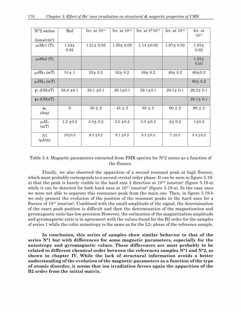
170 Chapter 5: Effect of He+ ions irradiation on structural & magnetic properties of CMS
N°2 series
(ions/cm2)
Ref Irr. at 1014 Irr. at 1015 Irr. at 5*1015 Irr. at 1016 Irr. at
1017
µ0Ms1 (T) 1.24±
0.02
1.21± 0.02 1.20± 0.02 1.14 ±0.02 1.07± 0.02 1.03±
0.02
µ0Ms2 (T)
1.25±
0.03
µ0Hk1 (mT) 51± 1 52± 0.2 52± 0.2 49± 0.2 49± 0.2 60±0.2
µ0Hk2 (mT) 60± 0.2
𝜸1 (GHz/T) 28.8 ±0.1 29.1 ±0.1 29.1±0.1 29.1±0.1 29.1± 0.1 29.2± 0.1
𝜸2 (GHz/T) 28.7± 0.1
φu
(deg)
0 30 ± 2 45 ± 2 65 ± 2 60 ± 2 90 ± 2
µ0Hu
(mT)
1.2 ±0.2 3.5± 0.2 3.5 ±0.2 3.5 ±0.2 2± 0.2 1±0.2
A1
(pJ/m)
10±0.2 9.3 ±0.2 9.1 ±0.2 8.3 ±0.2 7 ±0.2 5.4 ±0.2
Table 5.4: Magnetic parameters extracted from FMR spectra for N°2 series as a function of
the fluence.
Finally, we also observed the apparition of a second resonant peak at high fluence,
which most probably corresponds to a second crystal order phase. It can be seen in figure 5.19-
a) that the peak is barely visible in the hard axis 2 direction at 1016 ions/cm² (figure 5.19-a)
while it can be detected for both hard axes at 1017 ions/cm² (figure 5.19-a). In the easy axes
we were not able to separate this resonance peak from the main one. Then, in figure 5.19-b
we only present the evolution of the position of the resonant peaks in the hard axes for a
fluence of 1017 ions/cm². Combined with the small amplitude of the signal, the determination
of the exact peak position is difficult and then the determination of the magnetization and
gyromagnetic ratio has low precision However, the estimation of the magnetization amplitude
and gyromagnetic ratio is in agreement with the values found for the B2 order for the samples
of series 1 while the cubic anisotropy is the same as for the L21 phase of the reference sample.
In conclusion, this series of samples show similar behavior to that of the
series N°1 but with differences for some magnetic parameters, especially for the
anisotropy and gyromagnetic values. These differences are most probably to be
related to different chemical order between the references samples N°1 and N°2, as
shown in chapter IV. While the lack of structural information avoids a better
understanding of the evolution of the magnetic parameters as a function of the type
of atomic disorder, it seems that ion irradiation favors again the apparition of the
B2 order from the initial matrix.

171
Figure 5.19: FMR absorption spectra comparison at 16 GHz of hard 1 and hard 2 axes of
N°2 series samples irradiated at 1016 and 1017 ions/cm2 in a). In b), the evolution of hard
axes resonant peaks of N°2 sample irradiated at 1017 ions/cm2.
Sample N°3 series:
As stated in chapter IV, the reference sample of this series exhibits a clear L21 crystal
order. However a very small additional peak was detected in the hard axis 2 direction (the
one supporting the uniaxial anisotropy) that we accounted for a second crystal order which is
most probably the B2 order, based on the results of the samples of series N°1. In the following
we will call this second peak the minority peak in reference to its very small amplitude.
The evolution of the FMR spectra with the ion fluence is shown in figure 5.20. In figure
5.20-a only the easy axis 1 is shown for clarity as the two easy axes resonance always
superposed at all fluence. In figure 5.20-b we show the evolution of the two hard axes. Clearly,
the uniaxial anisotropy in the hard axis is visible for all fluence. However, the main effect of
the irradiation is to switch the direction of the uniaxial anisotropy from the hard axis 2 to the
hard axis 1 at 1016 ions/cm².
We begin with the effect of ion irradiation on the magnetic properties of the main L21
phase. Examples of fres Vs 𝜇0H0 curves for the main peaks are presented in figure 5.21. The
values of the magnetic parameters extracted from this curves are summarized in table 5.5.
We found typically two different behaviors depending on the ion fluence.
For 1014 and 1015 ions/cm², we observe a decrease of the magnetization amplitude and
exchange constant. The values of the magnetization and exchange are roughly similar to the
ones reported for L21 order of the samples of series N°1 at similar fluence. In addition the
values of the cubic anisotropy are roughly constant at these fluence, as for sample of series
N°1 and N°2, while the gyromagnetic constant slightly increases. This is similar to the
situation encountered for the sample N°2 and is maybe due to the higher rate of Co/Si
exchange observed for this sample as compared to the series N°1. Also the uniaxial anisotropy
stays always aligned with hard axis 2 direction but its amplitude slightly decreases. We
attribute this decrease to the fact that the out of plane lattice parameter of the reference
sample of series N°3 corresponds to the maximum value of the sample irradiated at 1016
ions/cm² of the series N°1. Then we think that the sample of series N°3 has already overpassed
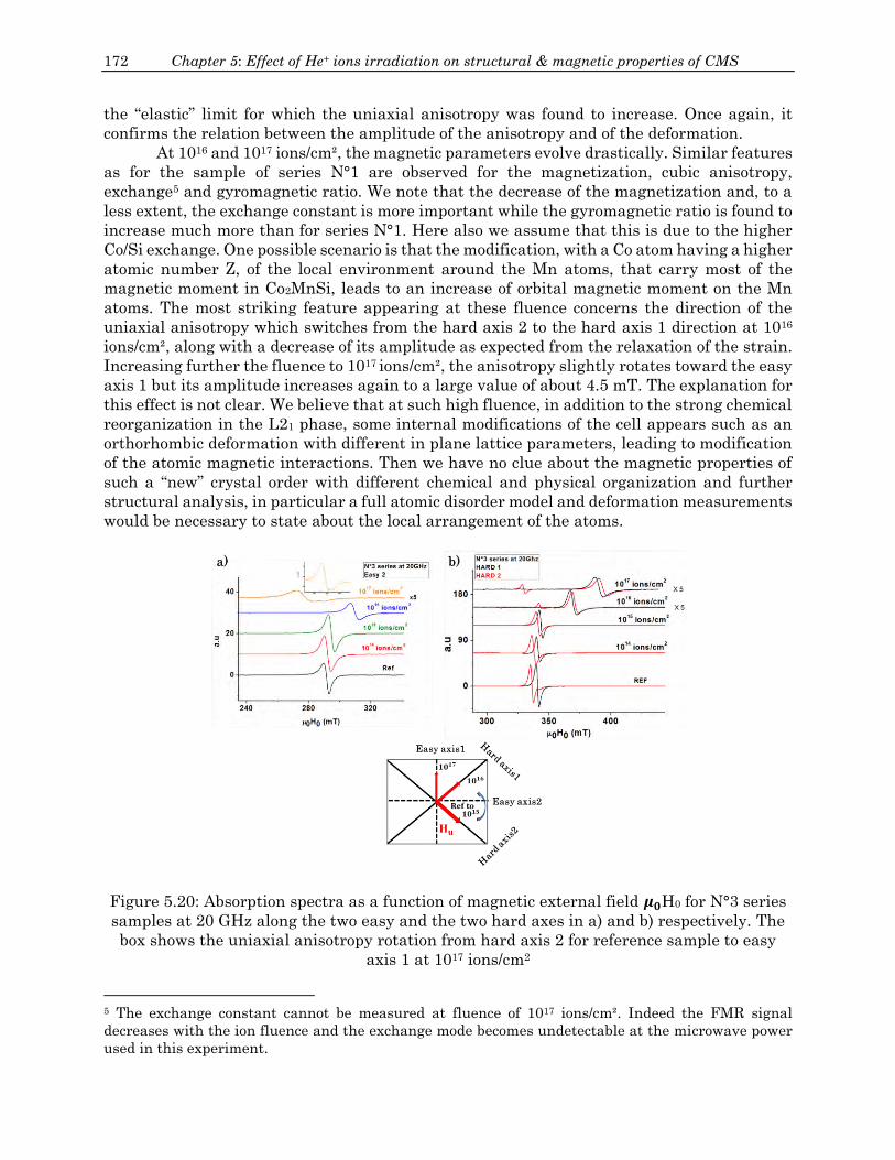
172 Chapter 5: Effect of He+ ions irradiation on structural & magnetic properties of CMS
the “elastic” limit for which the uniaxial anisotropy was found to increase. Once again, it
confirms the relation between the amplitude of the anisotropy and of the deformation.
At 1016 and 1017 ions/cm², the magnetic parameters evolve drastically. Similar features
as for the sample of series N°1 are observed for the magnetization, cubic anisotropy,
exchange5 and gyromagnetic ratio. We note that the decrease of the magnetization and, to a
less extent, the exchange constant is more important while the gyromagnetic ratio is found to
increase much more than for series N°1. Here also we assume that this is due to the higher
Co/Si exchange. One possible scenario is that the modification, with a Co atom having a higher
atomic number Z, of the local environment around the Mn atoms, that carry most of the
magnetic moment in Co2MnSi, leads to an increase of orbital magnetic moment on the Mn
atoms. The most striking feature appearing at these fluence concerns the direction of the
uniaxial anisotropy which switches from the hard axis 2 to the hard axis 1 direction at 1016
ions/cm², along with a decrease of its amplitude as expected from the relaxation of the strain.
Increasing further the fluence to 1017 ions/cm², the anisotropy slightly rotates toward the easy
axis 1 but its amplitude increases again to a large value of about 4.5 mT. The explanation for
this effect is not clear. We believe that at such high fluence, in addition to the strong chemical
reorganization in the L21 phase, some internal modifications of the cell appears such as an
orthorhombic deformation with different in plane lattice parameters, leading to modification
of the atomic magnetic interactions. Then we have no clue about the magnetic properties of
such a “new” crystal order with different chemical and physical organization and further
structural analysis, in particular a full atomic disorder model and deformation measurements
would be necessary to state about the local arrangement of the atoms.
Figure 5.20: Absorption spectra as a function of magnetic external field 𝝁𝟎H0 for N°3 series
samples at 20 GHz along the two easy and the two hard axes in a) and b) respectively. The
box shows the uniaxial anisotropy rotation from hard axis 2 for reference sample to easy
axis 1 at 1017 ions/cm2
5 The exchange constant cannot be measured at fluence of 1017 ions/cm². Indeed the FMR signal
decreases with the ion fluence and the exchange mode becomes undetectable at the microwave power
used in this experiment.

173
Figure 5.21: 𝒇𝒓𝒆𝒔 vs. 𝝁𝟎H0 curves for N°3 series for reference in a) and irradiated samples at
1015, 1016 and 1017 ions/cm2 in b), c) and d) respectively.
Now let’s return to the behavior of the minority peaks as a function of the ion fluence.
Between 1014 and 1016 ions/cm², we are not able to detect it anymore, neither in hard axis 2
nor in easy axis 1 (as for the reference sample). Most probably because it is mixed up with the
majority peak. Reaching 1016 ions/cm², it is visible again in the hard axis 2 direction.
Increasing further the fluence to 1017, both peaks become detectable in the hard axis 2 and
easy axis 1 directions, as for the reference sample. This is shown in figures 5.22-a and 5.22-b.
Likewise the samples of N°1 series, here we were not able to detect the second peak for the
two other magnetic directions. At this point we are not able to explain why we cannot observe
it in the four directions. Interestingly, the resonance field for the minority peak at fluence of
1017 is similar to the one of the reference sample. From the fres vs. 𝜇0H0 curve at 1017 ions/cm²
(Figure 5.22-c) we extract the magnetic parameters of this phase. We find that they are very
close to the magnetic parameters of the reference sample) initial crystal order. As for N°1
series, we believe that it corresponds to the reinforcement of the B2 order, which would also
show a small amount of Co-Si disorder as its magnetization amplitude is slightly lower than
for the N°1 series.
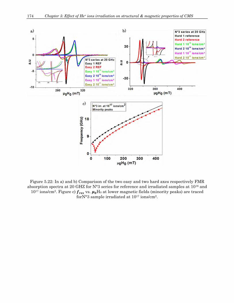
174 Chapter 5: Effect of He+ ions irradiation on structural & magnetic properties of CMS
Figure 5.22: In a) and b) Comparison of the two easy and two hard axes respectively FMR
absorption spectra at 20 GHZ for N°3 series for reference and irradiated samples at 1016 and
1017 ions/cm2. Figure c) 𝒇𝒓𝒆𝒔 vs. 𝝁𝟎H0 at lower magnetic fields (minority peaks) are traced
forN°3 sample irradiated at 1017 ions/cm2.

175
N°3 series
(ions/cm2)
Ref Irr. at 1014 Irr. at 1015 Irr. at 1016 Irr. at
1017
µ0Ms1 (T) 1.25
±0.02
1.24±0.02 1.21± 0.02 1.06± 0.02 1.02±
0.02
µ0Ms2 (T)
1.24
±0.02
µ0Hk1 (mT) 28± 0.5 28±0.5 28± 0.5 36.5 ± 0.5 69 ± 0.5
µ0Hk2 (mT) 25.5 ±0.5
𝜸1 (GHz/T) 28.7± 0.1 28.8± 0.1 28.85 ±
0.1
29.4 ± 0.1 30.2 ±0.1
𝜸2 (GHz/T) 28.7 ±0.2
φu
(deg)
45 ±1 45 ±1 45 ± 1 135 ±1 140 ±2
µ0Hu
(mT)
2 ± 0.2 1.8 ±0.2 1.8 ± 0.2 1 ± 0.2 4.5 ±0.2
A1
(pJ/m)
18±0.1 18 ± 0.1 17.5± 0.1 12±0.1
Table 5.5: Magnetic parameters extracted from FMR spectra for N°3 series as a function of
the fluence.
In conclusion, The L21 order of this series of samples shows similar behavior for
the magnetic parameters than the samples of series N°1, even if the variations as a
function of the fluence are more pronounced here. Also, this series shows some
interesting behavior of the uniaxial anisotropy which has to be related to the cell
distortion induced by the irradiation, and also the chemical modification of the
main phase. A full understanding of the evolution of the magnetic parameters
implies a complete structural analysis for fluence above 1016 ions/cm².
It is very interesting as it allows to state about the structural origin of the
uniaxial anisotropy observed in many systems, especially in Co2MnSi or Co2FeSi
but most probably also for Iron and others that show cubic anisotropy. In addition
the fact that the amplitude of the anisotropy decreases at fluence above 1016
ions/cm² is also in agreement with a relaxation of the starin for high deformation
and high density of local defects.

176 Chapter 5: Effect of He+ ions irradiation on structural & magnetic properties of CMS
5.3.3 Effect of He+ irradiation on the Gilbert Damping
Sample N°1 series:
The study of the linewidth as a function of the ion fluence for the L21 and B2 order for
the series of N°1 sample is presented in figure 5.23. In this figure we only present the
evolution of the linewidth for the magnetic directions for which the two peaks are sufficiently
well resolved to avoid a too important uncertainty, as for example of strong mixing of the two
modes. This is why we do not show the linewidth of the B2 order in the easy directions for
fluence of 5*1015 ions/cm². The values of the damping factor with the extrinsic linewidth of
N°1 series are presented in table 5.6
Two main features are observed depending on the crystal order. For the B2 order, the
linewidth first decrease for a fluence of 1015 ions/cm², with a very clear improvement of the
extrinsic contribution ΔH0. It is also accompanied by an enhancement of the effective damping
coefficient, especially in the easy axis direction for which the value is almost divided by 2.
This behavior for relatively low fluence is most probably to be related to the improvement of
the long range order of the B2 phase as demonstrated by Gaier et al [10 Gaier]. As already
mentioned, irradiation acts similarly as a local temperature annealing at low fluences. Then,
as the size of the B2 crystallite grows, the coherence of the precession for this crystal phase
is improved, decreasing the extrinsic linewidth. Then we believe that it is the inhomogeneity
contribution (variation of µ0Ms, µ0Hk, crystallite size etc...) to the extrinsic damping coefficient
that decreases. For higher fluences, the damping coefficient is found to be roughly equivalent
as for the reference sample while the ΔH0 increases. This is in agreement with the inclusion
of local point defects induced by the irradiation which is probably at the origin of two magnons
scattering process.
For the L21 phase, the situation is different. Irradiation is found to increase both the
effective damping coefficient and the ΔH0 contribution for the easy and the hard axis
directions. The increase of the extrinsic contribution is most probably of the same origin as
for the B2 order. However, the origin of the evolution of the intrinsic contribution 𝛼 is most
probably to be related to the chemical disorder in the matrix. Indeed, the 𝛼 parameter is
strongly dependent on the local atomic arrangement as it can modify either the spin-orbit
mediated relaxation mechanisms (see chap II) or the orbital and spin magnetic moments and
then the g values for example. We recall that in the Kamberský model of relaxation in
ferromagnets [13, 14 Kamberský and 15 pelzl], the damping coefficient is related to the
Gilbert relaxation coefficient G through the relation 𝛼=G*4𝜋/(µ0Ms𝛾). In addition, the Gilbert
damping coefficient G depends on the g value and on the spin-orbit coupling coefficient λSO
through the relation 𝐺𝑜𝑠 = (𝛾ℏ/2)2𝑍𝑓𝜆𝑠𝑜
2 (𝑔 − 2)2𝜏. In figure 5.24, we report on the evolution of
the Gilbert damping constant G as a function of (g-2)² calculated with the values of table 5.3.
For this crystal order, the g value increases for all fluences. Of course, we have only a few
points but we can see that either for the easy or hard axis, the relation is almost linear,
meaning that the amplitude of the spin-orbit coupling λSO is probably constant with the ion
fluence. This result shows that the damping coefficient is here dominated by spin-orbit
interaction without spin-flip interaction (what is called ordinary damping in the Kamberský
model).
This interesting result has to be emphasized on as one could expect some spin flip
scattering at the Fermi level. Indeed, the decrease of the magnetization amplitude was
accounted for a the Co/Mn exchange and so on the closure of the energy band gap for spin up
and spin down states. This result also impacts the understanding of the evolution of the
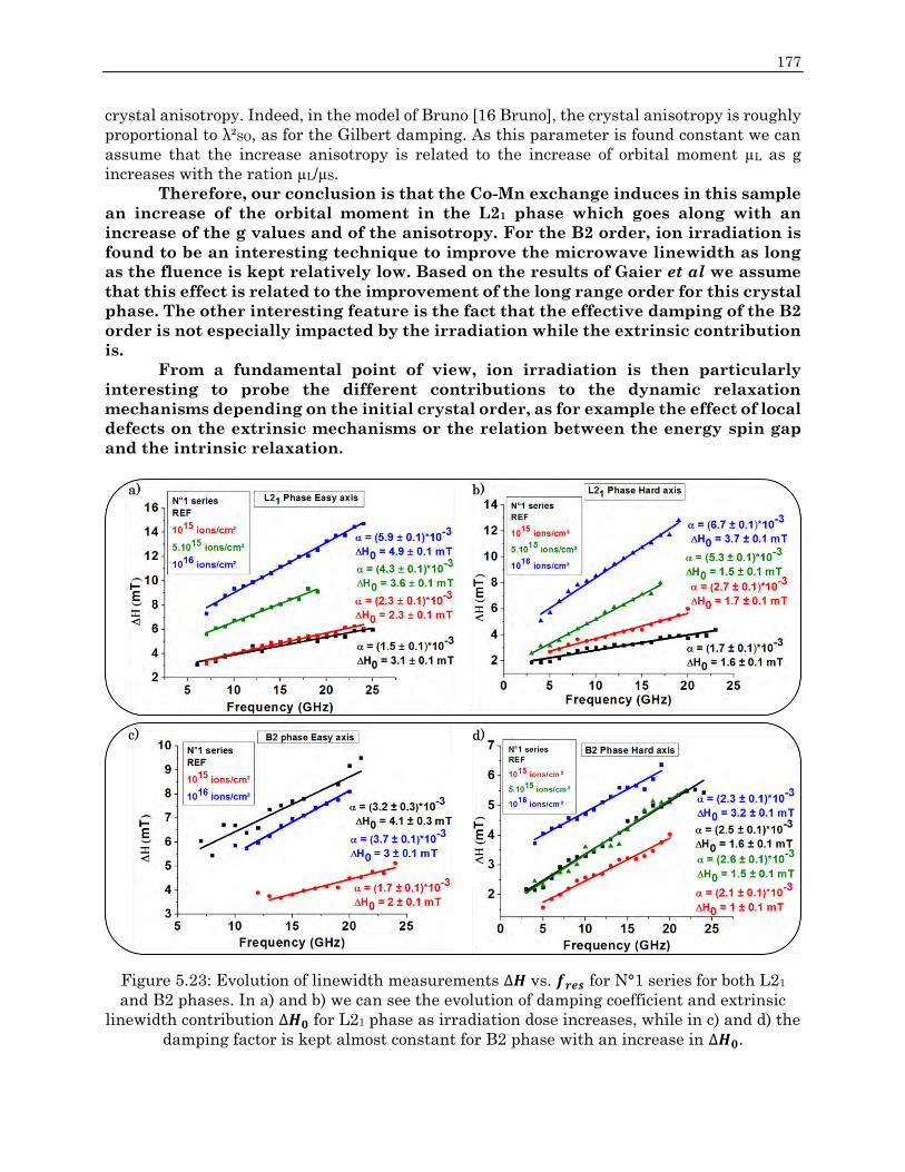
177
crystal anisotropy. Indeed, in the model of Bruno [16 Bruno], the crystal anisotropy is roughly
proportional to λ²SO, as for the Gilbert damping. As this parameter is found constant we can
assume that the increase anisotropy is related to the increase of orbital moment µL as g
increases with the ration µL/µS.
Therefore, our conclusion is that the Co-Mn exchange induces in this sample
an increase of the orbital moment in the L21 phase which goes along with an
increase of the g values and of the anisotropy. For the B2 order, ion irradiation is
found to be an interesting technique to improve the microwave linewidth as long
as the fluence is kept relatively low. Based on the results of Gaier et al we assume
that this effect is related to the improvement of the long range order for this crystal
phase. The other interesting feature is the fact that the effective damping of the B2
order is not especially impacted by the irradiation while the extrinsic contribution
is.
From a fundamental point of view, ion irradiation is then particularly
interesting to probe the different contributions to the dynamic relaxation
mechanisms depending on the initial crystal order, as for example the effect of local
defects on the extrinsic mechanisms or the relation between the energy spin gap
and the intrinsic relaxation.
Figure 5.23: Evolution of linewidth measurements ∆𝑯 vs. 𝒇𝒓𝒆𝒔 for N°1 series for both L21
and B2 phases. In a) and b) we can see the evolution of damping coefficient and extrinsic
linewidth contribution ∆𝑯𝟎 for L21 phase as irradiation dose increases, while in c) and d) the
damping factor is kept almost constant for B2 phase with an increase in ∆𝑯𝟎.

178 Chapter 5: Effect of He+ ions irradiation on structural & magnetic properties of CMS
N°1 series
ions/cm2
L21 Easy axis B2 Easy axis L21 Hard axis B2 Hard axis
Ref 𝜶 = (1.5±𝟎. 𝟏)*10-3 ∆𝑯𝟎 = 𝟑. 𝟏 𝐦𝐓
𝜶 =
(3.2±𝟎. 𝟑)*10-3
∆𝑯𝟎 = 𝟒. 𝟏 𝐦𝐓
𝜶 = (1.7±𝟎. 𝟏)*10-
3 ∆𝑯𝟎 = 𝟏. 𝟔 𝐦𝐓
𝜶 = (2.5±𝟎. 𝟏)*10-3 ∆𝑯𝟎 = 𝟏. 𝟔 𝐦𝐓
Irr. at 1015
𝜶 = (2.3±𝟎. 𝟏)*10-3
∆𝑯𝟎 = 𝟐. 𝟑 𝐦𝐓
𝜶 =
(1.7±𝟎. 𝟏)*10-3 ∆𝑯𝟎 = 𝟐 𝐦𝐓
𝜶 = (2.7±𝟎. 𝟏)*10-
3 ∆𝑯𝟎 = 𝟏. 𝟕 𝐦𝐓
𝜶 = (2.1±𝟎. 𝟏)*10-3
∆𝑯𝟎 = 𝟏 𝐦𝐓
Irr. at 5*1015
𝜶 = (4.3±𝟎. 𝟏)*10-3
∆𝑯𝟎 = 𝟑. 𝟔 𝐦𝐓
- 𝜶 = (5.3±𝟎. 𝟏)*10-
3 ∆𝑯𝟎 = 𝟏. 𝟓 𝐦𝐓
𝜶 = (2.6±𝟎. 𝟏)*10-3
∆𝑯𝟎 = 𝟏. 𝟓 𝐦𝐓
Irr. at 1016
𝜶 = (5.9±𝟎. 𝟏)*10-3
∆𝑯𝟎 = 𝟒. 𝟗 𝐦𝐓
𝜶 =
(3.7±𝟎. 𝟏)*10-3 ∆𝑯𝟎 = 𝟑 𝐦𝐓
𝜶 = (6.7±𝟎. 𝟏)*10-
3 ∆𝑯𝟎 = 𝟑. 𝟕 𝐦𝐓
𝜶 = (2.3±𝟎. 𝟏)*10-3
∆𝑯𝟎 = 𝟑. 𝟐 𝐦𝐓
Table 5.6: damping factor 𝛂 and extrinsic line width ∆𝐇𝟎 values for both one easy and one
hard axis of L21 and B2 phases in the series of sample N°1 reference and irradiated
samples.
Figure 5.24: Gilbert coefficient G/𝝀𝑺𝑶𝟐 as a function of (g-2)² for the L21 order in the easy
(black) and hard (red) directions. The values given on the graph corresponds to the different
fluence at which (g-2)² has been calculated.
.
Sample N°2 series:
The evolution of the linewidth for each magnetic direction as a function of the fluence
is shown in figure 5.25. Basically, the damping coefficient in every direction is found to be

179
roughly constant for fluence up to 5*1015 ions/cm², similarly as for the B2 crystal order of
series N°1. However, it increases at higher fluence, as for the L21 crystal order in series N°1.
This behavior is similar to the one observed for the samples of series N°3 (see below). The
increase at high fluence is most probably to be related to the strong increase of the atomic
disorder above 5*1015 in agreement with the sharp decrease of the magnetization of the L21
phase. Concerning the extrinsic contribution ΔH0, it is found to increase with the ion fluence,
especially above 5*1015, in agreement with enhanced scattering events due to the increased
density of defects.
We also notice that for fluences of 1014 and 1015 ions/cm², for which the internal
structure is barely modified, the damping coefficient is found to improve in the hard 1
direction as compared to the reference sample but the ΔH0 is at the same time increased by
almost a factor of two. The observed difference of 𝛼 are well above the uncertainty of the
measurement. However, the origin of this effect is not clear. Indeed, we know that the order
of the L21 phase is not improved at this fluence since the magnetization amplitude decreases.
So the improvement of α cannot be related to some improvement of the chemical ordering. If
the origin relies on inhomogeneity in the samples, both the ΔH0 and α would show the same
behavior, which is not the case. It is also particularly surprising that such effect appears only
in one direction. It is maybe to be related to the rotation of the uniaxial anisotropy toward the
hard axis 1 at 1015 ions/cm² meaning that mechanical strain could plays a role in the
amplitude of the intrinsic damping in Co2MnSi. However, further experiments are needed to
validate this hypothesis, especially phi scans that are not performed on the irradiated
samples of this series.
In conclusion, as compared to the series of sample N°1, the series of N°2
shows some feature similar to the B2 and L21 crystal order. Additionally, it is
possible that the presence of the uniaxial anisotropy modifies the intrinsic
damping in particular magnetic axis. However, the global behavior at high fluence
is in agreement with the first series.

180 Chapter 5: Effect of He+ ions irradiation on structural & magnetic properties of CMS
Figure 5.25: Evolution of damping coefficient and extrinsic linewidth contribution ∆𝑯𝟎 as a
function of irradiation dose from ∆𝑯 vs. 𝒇𝒓𝒆𝒔 measurements for N°2 series along the two easy
and two hard axes.
Finally we compare, the value of the linewidths in the hard axes direction for the two
modes observed at 1017 ions/cm². We clearly observe, in Figure 5.26, that the second phase
presents a lower linewidth with lower damping and ΔH0, as expected from the improvement
of B2 order. However, the values of the damping are higher than for the samples of series N°1
exhibiting clear B2 order. This is in agreement with our assumption that this sample exhibit
Co/Si exchange even in the B2 phase. The damping factor and extrinsic line width values of
N°2 are presented in Table 5.7.

181
Figure 5.26: Comparison between the two phases in hard axis 1 and 2 for sample N°2
irradiated at 1017 ions/cm2 as the damping factor 𝜶 and extrinsic linewidth ∆𝑯𝟎 is lower for
the second phase than the main phase.
N°2 series
(ions/cm2)
Easy axis1 Easy axis 2 Hard axis 1 Hard axis 2
Ref 𝜶 = (2.8±𝟎. 𝟏)*10-3 ∆𝑯𝟎 = 𝟐. 𝟑 𝐦𝐓
𝜶 = (3.2±𝟎. 𝟑)*10-3 ∆𝑯𝟎 = 𝟏. 𝟗 𝐦𝐓
𝜶 = (3.5±𝟎. 𝟏)*10-3 ∆𝑯𝟎 = 𝟏. 𝟑 𝐦𝐓
𝜶 =(2.3±𝟎. 𝟏)*10-3 ∆𝑯𝟎 = 𝟐. 𝟒 𝐦𝐓
Irr. at 1014
𝜶 = (2.6±𝟎. 𝟏)*10-3
∆𝑯𝟎 = 𝟐. 𝟓 𝐦𝐓
𝜶 = (3±𝟎. 𝟏)*10-3
∆𝑯𝟎 = 𝟐. 𝟕 𝐦𝐓
𝜶 = (2.6±𝟎. 𝟏)*10-3
∆𝑯𝟎 = 𝟐. 𝟔 𝐦𝐓
-
Irr. at 1015
𝜶 = (2.6±𝟎. 𝟏)*10-3 ∆𝑯𝟎 = 𝟐. 𝟗 𝐦𝐓
𝜶 = (2.7±𝟎. 𝟏)*10-3 ∆𝑯𝟎 = 𝟐 𝐦𝐓
(2.4±𝟎. 𝟏)*10-3 ∆𝑯𝟎 = 𝟐. 𝟑 𝐦𝐓
𝜶 =(2.5±𝟎. 𝟏)*10-3 ∆𝑯𝟎 = 𝟐. 𝟒 𝐦𝐓
Irr. at 5*1015
𝜶 = (3.4±𝟎. 𝟏)*10-3
∆𝑯𝟎 = 𝟐. 𝟒 𝐦𝐓
𝜶 = (3.7±𝟎. 𝟏)*10-3
∆𝑯𝟎 = 𝟐. 𝟔 𝐦𝐓
𝜶 = (2.6±𝟎. 𝟏)*10-3
∆𝑯𝟎 = 𝟐. 𝟔 𝐦𝐓
𝜶 =(2.5±𝟎. 𝟏)*10-3
∆𝑯𝟎 = 𝟐. 𝟔 𝐦𝐓
Irr. at 1016
𝜶 = (4.7±𝟎. 𝟏)*10-3 ∆𝑯𝟎 = 𝟑. 𝟔 𝐦𝐓
𝜶 = (4.8±𝟎. 𝟑)*10-3 ∆𝑯𝟎 = 𝟑. 𝟑 𝐦𝐓
𝜶 = (5.1±𝟎. 𝟏)*10-3 ∆𝑯𝟎 = 𝟐. 𝟒 𝐦𝐓
𝜶 =(5.1±𝟎. 𝟏)*10-3 ∆𝑯𝟎 = 𝟐. 𝟖 𝐦𝐓
Irr. at 1017
𝜶 = (4.7±𝟎. 𝟏)*10-3 ∆𝑯𝟎 = 𝟒. 𝟑 𝐦𝐓
𝜶 = (4.6±𝟎. 𝟏)*10-3 ∆𝑯𝟎 = 𝟒. 𝟓 𝐦𝐓
𝜶 = (5.5±𝟎. 𝟏)*10-3 ∆𝑯𝟎 = 𝟑. 𝟕 𝐦𝐓
𝜶 =(6.1±𝟎. 𝟏)*10-3 ∆𝑯𝟎 = 𝟑. 𝟒 𝐦𝐓
Table 5.7: damping factor 𝜶 and extrinsic line width contribution ∆𝑯𝟎 values for N°2 series
reference and irradiated samples along the two easy and two hard axes.

182 Chapter 5: Effect of He+ ions irradiation on structural & magnetic properties of CMS
Sample N°3 series:
For this series of sample we always observe that the linewidths for the easy axes are
bigger than for the hard axes whatever the ion fluence. This is shown in figure 5.27, which
presents the linewidths in the four magnetic directions at different fluence for the L21 order.
Moreover the easy axis 2 shows higher linewidth and effective damping than the easy axis 1,
except at 1016 and 1017 ions/cm² for which the situation is inversed.
Figure 5.27: ∆𝑯 vs. 𝒇𝒓𝒆𝒔 measurements of N°3 series irradiated samples from 1014 to 1017
ions/cm2 along the 4 axes directions shows clearly that the easy axes have higher ∆𝑯 than
hard axes.
In figure 5.28 we present the evolution of the linewidth in each magnetic direction as
a function of the ion fluence of sample N°3 series. Same general tendencies as for the samples
of series N°1 and N°2 are visible, i.e., an increase of the effective damping coefficient and
extrinsic contribution ΔH0 with the ion fluence up to 1016 ions/cm². However at 1017, the
damping coefficient tends to saturate while the ΔH0 becomes very important, the latter point
being in agreement with the expectation of the TRIM simulations (figure 5.3).
At 1014 and 1015 ions/cm², the evolution of the linewidth is similar to the situation
encountered for the samples of series N°2. Indeed for all directions, the linewidths are roughly

183
similar as a function of the fluence, except for the hard axis 2 for which a clear increase at
1014 of the 𝛼 is observed. This increase is accounted for the mixing of the L21 and B2 resonance
at this fluence, as shown in figure 5.20-b. The values of damping factor and extrinsic line
width of N°3 are presented in Table 5.8.
At 1016 some particular feature appears. In addition to the fact that the linewidth of
the easy axis 1 becomes more important than the linewidth of the easy axis 2, we observe that
the increase damping coefficient for the hard and easy axes 1 increase much more than the
one of the hard and easy axes 2. Interestingly this change arises for the fluence for which the
uniaxial anisotropy is found to switch from one hard axis to the other. It is possible that this
measurement shows the effect of the mechanical deformation of the value of the intrinsic
damping in the Co2MnSi. However this tendency is not observed anymore at 1017 ions/cm².
Maybe it is due to the fact that the material has suffered strong internal chemical and
mechanical deformation at this fluence, changing drastically the relaxation mechanisms.
Then it is possible that this measurement shows the effect of the mechanical deformation of
the value of the intrinsic damping in the Co2MnSi but it is very difficult to conclude of this
point as the effect at very high fluence does not confirm the tendency. Further measurements
at some intermediate fluence between 5*1015 and 1017 should be necessary to follow the
evolution of the damping with more precision. Also, a full structural characterization of the
lattice parameter and deformation is needed.
As the gyromagnetic ratio and cubic anisotropy were found to increase with the
fluence, we also studied the evolution of G/𝝀𝑺𝑶𝟐 as a function of (g-2)². The result is shown in
Figure 5.29 for fluence up to 1016 ions/cm². We consider only the L21 crystal order and we
compare it with the one calculated for the samples of series N°1 and N°3 in the hard axis.
Clearly, for the sample of series N°3, we do not observe the same linear variation as for series
N°1. This demonstrates that the damping is not governed only by ordinary scattering in this
sample and spin flip scattering processes are allowed. The difference between the series N°1
and N°3 may have to be related to the different Co/Si exchange that arises for sample N°3,
meaning that this kind of disorder strongly modifies the intrinsic relaxation mechanisms.

184 Chapter 5: Effect of He+ ions irradiation on structural & magnetic properties of CMS
Figure 5.28: Evolution of damping coefficient and extrinsic linewidth contribution ∆𝑯𝟎 as a
function of irradiation dose from ∆𝑯 vs. 𝒇𝒓𝒆𝒔 measurements for N°3 series along the two easy
and two hard axes.
Figure 5.29: A comparison between the evolution of G/𝝀𝑺𝑶𝟐 as a function of (g-2)² along one
hard axis for N°1 series and two hard axis for N°3 series.

185
Finally, the values of the linewidth for the two crystal orders at 1017 ions/cm² in figure
5.30 are compared. Clearly, the expected B2 order shows much narrower linewidths as
compared to the main phase. Indeed, we find some values of the effective damping down to
1.5*10-3 in the hard axis direction, which is very good taking into account the induced disorder
by irradiation.
N°3 series
ions/cm2
Easy axis1 Easy axis 2 Hard axis 1 Hard axis 2
Ref 𝜶 =(3±𝟎. 𝟏)*10-3
∆𝑯𝟎 = 𝟏. 𝟗 𝐦𝐓
𝜶 =(3.𝟒 ± 𝟎. 𝟏)*10-3
∆𝑯𝟎 = 𝟐. 𝟐 𝐦𝐓
𝜶 = (1.9±𝟎. 𝟏)*10-3
∆𝑯𝟎 = 𝟏. 𝟓 𝐦𝐓
𝜶 =(2.1±𝟎. 𝟏)*10-3
∆𝑯𝟎 = 𝟏. 𝟒 𝐦𝐓
Irr. at 1014
𝜶 = (3.5±𝟎. 𝟏)*10-3
∆𝑯𝟎 = 𝟐. 𝟓 𝐦𝐓
𝜶 = (4±𝟎. 𝟏)*10-3
∆𝑯𝟎 = 𝟐. 𝟐 𝐦𝐓
𝜶 = (2.3±𝟎. 𝟏)*10-3
∆𝑯𝟎 = 𝟐 𝐦𝐓
𝜶 =(3.2±𝟎. 𝟏)*10-3
∆𝑯𝟎 = 𝟏. 𝟏 𝐦𝐓
Irr. at 1015
𝜶 = (3.5±𝟎. 𝟏)*10-3
∆𝑯𝟎 = 𝟐. 𝟒 𝐦𝐓
𝜶 =(5.3±𝟎. 𝟏)*10-3
∆𝑯𝟎 = 𝟏. 𝟖 𝐦𝐓
(1.7±𝟎. 𝟏)*10-3
∆𝑯𝟎 = 𝟐. 𝟑 𝐦𝐓
𝜶 =(3.8±𝟎. 𝟏)*10-3
∆𝑯𝟎 = 𝟎. 𝟖 𝐦𝐓
Irr. at 1016
𝜶 = (5±𝟎. 𝟏)*10-3 ∆𝑯𝟎 = 𝟐. 𝟕 𝐦𝐓
𝜶 =(6.𝟔 ± 𝟎. 𝟏)*10-3 ∆𝑯𝟎 = 𝟑 𝐦𝐓
𝜶 = (5.7±𝟎. 𝟏)*10-3 ∆𝑯𝟎 = 𝟏. 𝟑 𝐦𝐓
𝜶 =(4.9±𝟎. 𝟏)*10-3 ∆𝑯𝟎 = 𝟏. 𝟔 𝐦𝐓
Irr. at 1017
𝜶 = (5±𝟎. 𝟏)*10-3 ∆𝑯𝟎 = 𝟏𝟐. 𝟓 𝐦𝐓
𝜶 = (5.5±𝟎. 𝟏)*10-3 ∆𝑯𝟎 = 𝟗. 𝟓 𝐦𝐓
𝜶 = (4.2±𝟎. 𝟐)*10-3 ∆𝑯𝟎 = 𝟔 𝐦𝐓
𝜶 =(5.3±𝟎. 𝟑)*10-3 ∆𝑯𝟎 = 𝟓. 𝟑 𝐦𝐓
Table 5.8: damping factor 𝜶 and extrinsic line width ∆𝑯𝟎 values for N°3 series reference and
irradiated samples along the two easy and two hard axes.
Figure 5.30: A comparison of the damping factor 𝜶 and the linewidth ∆𝐻0 for two crystal
order of N°3 sample irradiated at 1017 ions/cm2.

186 Chapter 5: Effect of He+ ions irradiation on structural & magnetic properties of CMS
In conclusion, this series of samples shows similar behavior as the sample of series
N°1 and N°2 with an increased intrinsic and extrinsic contribution at fluence above 1016
ions/cm². However the study of the Gilbert coefficient shows that relaxation mechanisms must
differ in this series as compared to the series N°1. We also observed that the intrinsic damping
of the B2 order induced by ion irradiation is much lower than for the modified L21’ phase, as
we reach values of 1.5*10-3 in the hard axis direction. Finally, it is possible that the
mechanical strain play a role in the value of the damping coefficient but further experiments
at intermediate fluence are required to validate our assumption.
Conclusion
In conclusion, we have presented three series of samples which shows different magnetic
behaviors and different initial atomic disorder. The main observations are summarized below:
- Structural analysis performed by X-ray and HAADF-STEM imaging have shown that
ion irradiation induces atomic disorder in Co2MnSi alloys, especially for fluence above
5*1015 ions/cm². For the three series of samples we assume that ion irradiation favors
the B2 crystal order to the cost of the L21 order. On the other hand, the structural
analysis performed on the series N°1 and N°3 shows that the L21 order is submitted
to a Co-Mn (D03 type) disorder and/or Co-Si exchange.
- Ion irradiation has been found to increase the out of plane lattice parameter of the
alloy. This induces a tetragonal (and maybe orthorhombic at fluence of 1017 ions/cm²
for the series N°3) distortion of the unit cell. At the same time, in each series of
samples, we observe the rotation and modification of the amplitude of the uniaxial
anisotropy when increasing the fluence, until the material is fully relaxed. Then we
believe that structural deformation and uniaxial anisotropy must be related, the latter
being a consequence of the mechanical strain induced by lattice deformation.
- The local defects induced by ion irradiation have been showed to increase the coercive
field of the samples of series N°1, meaning that the switching mechanism of this series
is governed by propagation effects.
- The static magnetic parameters (Ms, Hk, A) has been found to be unaffected by
irradiation for the B2 order. For the L21 order, ion irradiation induces a decrease of
the magnetization and exchange amplitude while the cubic anisotropy and
gyromagnetic ratio increases. We assume that it is due to the modification of the local
environment of the Mn atoms. We believe that atomic disorder on Co sites (i.e. Co/Mn
or Co/Si exchange) leads to a closing of the spin splitting at the Fermi level, inducing
a lower magnetization and exchange values, in agreement with theoretical predictions
in literature. Moreover the atomic disorder is assumed to increase the orbital moment
on the Mn atoms and the spin-orbit coupling, explaining the behavior of the
gyromagnetic ratio and anisotropy.
The effect of ion irradiation on the FMR linewidth has been found to depend on the initial
crystal order:
187
- For the B2 order, we observe on series N°1 a clear improvement of the extrinsic
contribution ΔH0 for fluence up to 1015 ions/cm², which is in agreement with previous
report by Gaier et al of the improvement of long range order in B2 phase at low fluence.
At higher fluence the ΔH0 increases in agreement with the creation of local defects
such as vacancies and interstitial in the alloy. We also observed that the effective
damping α was roughly constant, even at high fluence such as 1017 for the series N°2
and N°3. This means that most probably the B2 order is not summited to strong
chemical atomic disorder. On the samples of series N°2 and N°3, the value of the
effective damping of the expected B2 order at 1017 ions/cm² has been found in very good
agreement with the value of the B2 phase for the series N°1.
- For the L21 phase, the general tendency is an increase of the effective damping with
the fluence. This is in agreement with the reduced magnetization if spin-flip scattering
relaxation is allowed, and also with the increased spin-orbit interaction observed for
the cubic anisotropy. Beside this, the effective 𝛼 was found to be improved in the
direction of the uniaxial anisotropy for the series N°2 at low fluence, while it was
found to be degraded for the series N°3. Finally, we were not able to state about the
possible relation between the mechanical deformation induced in the matrix and the
evolution of the effective damping. Further studies such as angle dependence of the
linewidths, and measurements are intermediate fluence for which the relaxation
appear are required to conclude on this point.
Chapter 5 References:
[1] J. Fassbender, D. Ravelosona, et Y. Samson, « Tailoring magnetism by light-ion
irradiation », J. Phys. Appl. Phys., vol. 37, no 16, p. R179, août 2004.
[2] J. Fassbender et J. McCord, « Control of saturation magnetization, anisotropy, and
damping due to Ni implantation in thin Ni81Fe19 layers », Appl. Phys. Lett., vol. 88, no 25,
p. 252501, 2006.
[3] J. Fassbender, S. Poppe, T. Mewes, A. Mougin, B. Hillebrands, D. Engel, M. Jung, A.
Ehresmann, H. Schmoranzer, G. Faini, K. j. Kirk, et J. n. Chapman, « Magnetization
Reversal of Exchange Bias Double Layers Magnetically Patterned by Ion Irradiation »,
Phys. Status Solidi A, vol. 189, no 2, p. 439‑447, février 2002.
[4] D. Ravelosona, C. Chappert, H. Bernas, D. Halley, Y. Samson, et A. Marty, « Chemical
ordering at low temperatures in FePd films », J. Appl. Phys., vol. 91, p. 8082‑8084, 2002.
[5] D. Ravelosona, C. Chappert, V. Mathet, et H. Bernas, « Chemical order induced by ion
irradiation in FePt (001) films », Appl. Phys. Lett., vol. 76, no 2, p. 236, 2000.
[6] J. F. Ziegler et J. P. Biersack, « The Stopping and Range of Ions in Matter », in Treatise
on Heavy-Ion Science, D. A. Bromley, Éd. Springer US, 1985, p. 93‑129.
[7] « James Ziegler - SRIM & TRIM ». [En ligne]. Disponible sur: http://www.srim.org/.
[8] Radiation Effects and Defects in Solids: Incorporating Plasma Science and Plasma
Technology - Volume 141, Issue 1-4 .
[9] H. Bernas, J.-P. Attané, K.-H. Heinig, D. Halley, D. Ravelosona, A. Marty, P. Auric, C.
Chappert, et Y. Samson, « Ordering Intermetallic Alloys by Ion Irradiation: A Way to
Tailor Magnetic Media », Phys. Rev. Lett., vol. 91, no 7, août 2003.

188 Chapter 5: Effect of He+ ions irradiation on structural & magnetic properties of CMS
[10] S. Picozzi, A. Continenza, et A. Freeman, « Role of structural defects on the half-
metallic character of Co2MnGe and Co2MnSi Heusler alloys », Phys. Rev. B, vol. 69, no 9,
mars 2004.
[11] O. Gaier, J. Hamrle, B. Hillebrands, M. Kallmayer, P. Pörsch, G. Schönhense, H. J.
Elmers, J. Fassbender, A. Gloskovskii, C. A. Jenkins, C. Felser, E. Ikenaga, Y. Sakuraba,
S. Tsunegi, M. Oogane, et Y. Ando, « Improvement of structural, electronic, and magnetic
properties of Co2MnSi thin films by He+ irradiation », Appl. Phys. Lett., vol. 94, no 15, p.
152508, avr. 2009.
[12] A. Hubert and R. Schäfer, Magnetic domains: the analysis of magnetic microstructures.
Berlin ; New York: Springer, 1998.
[13] V. Kamberskỳ, « On ferromagnetic resonance damping in metals », Czechoslov. J.
Phys. B, vol. 26, no 12, p. 1366–1383, 1976.
[14] V. Kamberský, « Spin-orbital Gilbert damping in common magnetic metals », Phys.
Rev. B, vol. 76, no 13, oct. 2007.
[15] J. Pelzl, R. Meckenstock, D. Spoddig, F. Schreiber, J. Pflaum, et Z. Frait, « Spin–orbit-
coupling effects on g-value and damping factor of the ferromagnetic resonance in Co and
Fe films », J. Phys. Condens. Matter, vol. 15, no 5, p. S451, 2003.
[16] P. Bruno, «Tight-binding approach to the orbital magnetic moment and
magnetocrystalline anisotropy of transition-metal monolayers. Phys. Rev. B 39, 865
(1989).

189
Conclusion and Perspective
Heusler alloys are known to exhibit very special magnetic features, such as half
metallicity and low damping coefficient, as a function of the degree of atomic order in the
material. These properties are highly required for the development of spintronics devices
based on magnetoresistance or spin torque effects. In this work, we offered to get a deeper
insight into the correlation between the magnetic and structural properties of the Co2MnSi
alloy by studying the evolution of its static and dynamic magnetic parameters when
submitted to He+ ion irradiation at 150 KeV. Our work was based on the results obtained by
Gaier et al. showing that He+ ion irradiation at low fluences improves the long range B2 order
in Co2MnSi. In addition to the fundamental aspect of our approach, one of our goals was to
study the possibility of improving the atomic order, even in the L21 phase, and then
decreasing the dynamic damping of the material down to the theoretical predictions by Liu et
al. (~0.6 ∗ 10−4). Another goal was to study the effect of atomic disorder on the fundamental
dynamic relaxation mechanisms by a proper control of the structure of the material.
For this purpose, several experimental techniques have been combined. Structural
characterization has been achieved through X-ray diffraction in normal and anomalous
conditions for a quantitative description of atomic disorder, while electron microscopy and
especially HAADF-STEM imaging has been used to study the local organization of the atomic
structure. Beside this, ferromagnetic resonance, MOKE and PPMS magnetometry allowed
the determination of the static and dynamic magnetic parameters of the alloy. In this
manuscript, we have chosen to present the experimental results observed for three series of
samples. This choice is due to the difference of evolution of the structural and magnetic
properties for each series.
In chapter IV, we first studied the structure and the magnetic properties of the
reference samples of each series. Each sample is a thin film, with a thickness between 40 and
50 nm, grown on MgO substrate by sputtering. The CMS films verify the expected epitaxial
relationship (001)[110] // MgO(001)[100] ], indicating a 45° rotation of the CMS on the MgO
substrate in order to minimize the lattice mismatch. Moreover, GPA analysis, performed from
HAADF-STEM images, on the reference sample of series N°1 shows that the films are fully
relaxed.
One of the major results presented in this chapter is that the structure of the three
reference samples is slightly different. First, X-ray diffraction demonstrated that the unit cell
is tetragonal with an out-of-plane lattice parameter of 5.67 and 5.69 Ǻ for the reference
samples of series N°1 and N°3, respectively. Moreover, the chemical atomic disorder was
found to be different from one sample to the other. For example, the reference sample of series
N°1 exhibits small crystallites with B2 order inside a L21 matrix. The rate of Co-Si exchange
for this sample has been found to be below the uncertainty of the measurement, i.e. below 2%.
L21 order was also found for the reference sample of series N°3 but the Co-Si exchange rate
was found to be about 6% while no B2 order was observable in HAADF-STEM images. This
means that the B2 order is either absent or that crystallites are too small to induce a variation
of contrast in HAADF-STEM images. Unfortunately a complete structural analysis could not
be performed on the reference sample of series N°2. Only X-ray diffraction performed with a

190 Conclusion and perspective
diffractometer equipped for small samples has been carried out. A very small amplitude of
the (111) superlattice diffraction peak was observed for this sample. Based on the results
obtained for the two other samples, it is possible that it grows either mainly in the B2 phase
and/or in the L21 phase with strong Co-Si exchange.
The three reference samples also show different magnetic behaviors. For example, in
FMR measurements, the reference samples of series N°1 and N°3 exhibit two resonance
peaks, that we attribute to the L21 and B2 crystal order, while the reference sample of N°2
series exhibit only a single peak that we attributed to a disordered L21 phase. The values of
the magnetization, exchange and gyromagnetic ratio for the three samples are in good
agreement with reported values in the literature for L21 and B2 crystal order. One interesting
feature of our samples concerns the anisotropy. Indeed the amplitude of the cubic anisotropy
is more important than the one reported in literature for CMS deposited on MgO substrate.
In addition, we observe the presence of a small uniaxial anisotropy which is aligned either
with an easy axis for the samples of series N°1 and N°2 or with a hard axis for sample N°3.
The origin of this additional anisotropy is accounted for the out-of-plane deformation of the
unit cell but it is worth to mention that the effect of the chemical disorder cannot be
eliminated.
We also studied the FMR linewidth of the three samples. Interestingly, we observe an
anisotropic behavior of the linewidth and of the intrinsic damping coefficient. As explained in
chapter 4, we measure in fact an effective damping coefficient that takes into account several
contributions. Then further analytical analysis, especially taking into account the mosaicity
of the sample and the two magnon processes, is needed to state about the origin of this
anisotropy and conclude about an isotropic or anisotropic damping constant. One important
result of this chapter is that the best effective damping coefficient is found for the reference
sample of series N°1 for which we were able to separate the contribution of the B2 and the
L21 order. We obtained an effective damping down to 1.6*10-3, which is better than most of
the reported work up till now. Then, two main conclusions for this part can be emphasized
on. The first one is that the understanding of the magnetic behavior and the determination
of the static and dynamic parameters of the Co2MnSi must include a full structural analysis
of the material, including a study of the atomic disorder and mechanical strain in the
material. To our knowledge such kinds of studies are rarely performed. In addition, we believe
that the presence of the atomic disorder is at the origin for the reported values of 𝛼 in
literature which are generally between 6*10-3 and 3*10-3, almost one order of magnitude above
the theoretical predictions. In our case we also believe that the values of 𝛼 determined by the
ΔH vs. fres curves are the upper limit of the intrinsic coefficient, as many contributions to the
linewidth arise. Then, if improving the crystallinity of our samples, we could expect to reach
intrinsic damping coefficient down to 10-3, as recently reported by Andrieu et al. in Co2MnSi
grown by MBE on MgO substrate.
In chapter 5, we studied the effect of ion irradiation on the structural and magnetic
properties of the alloy. In the first part of this chapter we present simulations of the expected
damages induced by the irradiation. While these simulations give the order of magnitude of
the maximum damage that can be induced, it shows that local point defects such as vacancies
or interstitial cannot be neglected for fluence above 1016 ions/cm².
The effect of irradiation on the structure of the alloy is found to depend on the original
structure of the material. Indeed, for the samples of series N°1, we demonstrated that the
irradiation favors the B2 order to the cost of the L21 phase. In addition, Co-Mn exchange is
found to rise in the L21 matrix while Co-Si exchange is kept roughly constant up to 1016
ions/cm². The study of the magnetic parameters for the three series of samples makes us

191
believe that ion irradiation always favors the B2 order in every sample. This confirms the
result obtained by Gaier et al. For the samples of series N°3, only X-ray diffraction with a Cu
source have been performed so only the Co-Si exchange rate could be studied. We found a
strong increase of this parameter with the ion fluence. However, such atomic exchange was
not detected in the HAADF-STEM analysis. Indeed we observed a very uniform contrast,
similar to the one expected for B2 order. Therefore, we propose a scenario in which a double
exchange mechanism appears in the L21 matrix. We believe that Co-Mn and Mn-Si exchange
are first induced at low fluences, similarly as for N°1 series. Then we believe that it is the Co
atoms which are on the Mn sites that switch their position with Si atoms. Further structural
analysis will be needed to validate our assumption.
In addition to the chemical disorder, we observe that the irradiation increases the out-
of-plane lattice parameter of the samples of series N°1 and N°3. For the samples of series N°3
only the out-of-plane parameters have been measured due to the experimental configuration
of the diffractometer. However, for the series of sample N°1, we could verify that the in-plane
lattice parameters are kept constant for fluences up to 1016 ions/cm², meaning that the volume
of the unit cell (a²c) is not constant during the deformation.
The effect of the ion irradiation on the magnetic parameters of the alloy is presented
in the last part of chapter 5. We find two different effects depending on the crystal order. The
general tendencies are the following. Surprisingly the magnetic parameters of the B2 order
are almost constant whatever the fluence. The only effect of irradiation is an increase of the
extrinsic contributions ΔH0 to the FMR linewidth, in agreement with the increased numbers
of local defects. This again confirms that ion irradiation favors the B2 order in Co2MnSi. For
the L21 order the situation is different. Due to the induced atomic disorder, the values of the
magnetization and exchange are found to decrease, in agreement with theoretical predictions
of the loss of half metallicity with structural disorder. More interestingly we observed an
increase of the gyromagnetic ratio and cubic anisotropy which reflects an increase of the
orbital magnetic moment and spin-orbit interaction in the material.
In addition, one of the most striking features in our experiments is that the uniaxial
anisotropy is found to rotate in the plane of the layer when increasing the ion fluence.
Moreover its amplitude is found to increase for fluence up to 5*1015 ions/cm². At 1016 ions/cm²
the uniaxial anisotropy amplitude decreases. We believe that the increase of the anisotropy
amplitude is related to an elastic deformation of the unit cell when the decrease at 1016 can
be accounted for the relaxation of the internal strain, which can be mediated by the structural
defects induced by irradiation. Finally the anisotropy amplitude increases again for fluence
of 1017 ions/cm². For such high fluence, the strong internal modifications of the chemical order
along with some irreversible mechanical distortions (such as orthorhombic deformations for
example) have to be considered. The possibility offered by ion irradiation to follow the
evolution of the uniaxial anisotropy as a function of the deformation allows to clarify the
origin of the uniaxial anisotropy. This result is of particular interest since it can be extended
to other magnetic systems presenting the same behavior.
Finally, we studied the effect of ion irradiation on the linewidth of the different
samples. As already stated, the intrinsic effective damping for the B2 order seems to be
constant with the fluence. The extrinsic contributions were even found to be improved for the
samples of series N°1 at fluence below 1015 ions/cm², reflecting the improvement of the long
range order of this phase. For the L21 order, the general tendency is an increased of the
damping coefficient, especially at high fluence due to the modification of the local
environment around the Mn atoms. However, we also observed that for the samples of series
N°2 and N°3, there could be some relation between the evolution of the uniaxial anisotropy
and a potential improvement of the damping in some particular magnetic directions. This

192 Conclusion and perspective
appears only at fluence below 1015 ions/cm². At this point, it is not possible to state clearly on
this assumption. Additional experiments are needed. Especially it would be necessary to
study the linewidth in directions close to the direction of the uniaxial anisotropy.
Finally we would like to emphasize on some strange features observed for the second
resonant peak appearing in the samples of N°2 and N°3 series at high fluence, and to a less
extent in N°1 series. From the dispersion curves fres vs H0 in one easy and one hard axis
directions obtained for this resonance,, we deduced in agreement with the reported values
for a B2 order. However, this resonance shows strong variations of its amplitude depending
on the magnetic directions and ion fluence. It is even completely undetectable for two
directions for the samples of N°3 series. At the time we write this manuscript we do not have
any explanations for these observations.
In conclusion, it is clear that ion irradiation at low fluences can be a very efficient tool
to improve the B2 order in Co2MnSi. This technique can be of particular interest since this
crystal order is supposed to show a half metallic behavior. Therefore, we believe that it can
be a credible complementary technique to temperature annealing to improve the order of this
crystal phase in Heusler alloy. We also demonstrated that the atomic disorder and maybe
mechanical strain are two key parameters to optimize the magnetic properties of Co2MnSi in
view of spintronic applications. While a much better control of the growing condition must be
fulfilled to get reproducible effects, the very low damping measured in our work demonstrates
the potential of Co2MnSi to develop low energy consumption microwave devices, or spin
torque memories. We believe that damping coefficient down to 10-3 or below are achievable in
a very “pure” crystal, making of this material one of the most interesting ferromagnetic
materials compatible with microelectronics processes.
From a fundamental point of view, ion irradiation is also very interesting to study
the effect of disorder on the dynamic relaxation mechanisms. For example, starting from a
thin film with B2 order, ion irradiation can be used to control the density of defects and
study the evolution of the extrinsic contributions to the linewidth. The main interest being
that, all the other magnetic parameters would be kept constant. It is also an interesting
technique to probe fundamental interaction in the material such as the correlation between
the spin-orbit interaction and the intrinsic damping coefficient. In this work we only get
very preliminary results on this entanglement for N°1 series samples. In addition, ion
irradiation offers the possibility to study the spin-flip and non spin-flip relaxation
mechanisms by controlling the atomic disorder, and so the energy bandgap for spin up and
spin down, in the material. For this the best configuration would be to start with a single
crystal of L21 order. The main difficulty encountered in our work to get a deeper
understanding of these different contributions was to separate the contributions to the
linewidth of the different crystal order present in the as deposited material. One key issue
for the future of this work will be the improvement of deposition condition to reduce the
atomic disorder and phase mixing in the alloy.

Sommaire Thèse
Les matériaux demi-métalliques sont aujourd’hui particulièrement attractif pour les
dispositifs à électronique de spin ainsi que les dispositifs micro-ondes.. Ces matériaux ont une
propriété unique, ils se comportent comme métal pour une orientation du spin et en tant que
semi-conducteur pour l'autre avec un écart au niveau de fermi qui conduit à une polarisation
de spin de 100%. Un exemple de de matériaux demi-métalliques est la famille des alliages d’
Heusler. Ces alliages ont été découverts en 1903 par F. Heusler [1 Heusler] en combinant 3
éléments non magnétiques tel que Cu2MnAl qui se comporte comme un matériau
ferromagnétique. Après cette découverte, de nombreux autres composés ont également été
ajoutés à cette famille. En 1983, De Groot et al. [2 De Groot] ont montré le comportement
demi-métallique du composé NiMnSb; cette découverte a conduit à un grand intérêt pour
l'étude des alliages Heusler. Une autre propriété importante, qui est d'un intérêt particulier
dans ce manuscrit de thèse, est le faible coefficient d'amortissement Gilbert dans ces
composés qui est prévu pour être en dessous de 10-3 dans certains cas comme le Co2MnSi, soit
un ordre de grandeur environ meilleur que la plupart des métaux ferromagnétiques
classiques. La combinaison de la polarisation en spin et du faible amortissement de Gilbert
sont importants pour le retournement de l'aimantation dans les dispositifs STT MRAM.
Depuis lors, diverses combinaisons atomiques ont été testées comme par exemple des
composés à base de cobalt Heusler. Au cours des 10 dernières années, le travail expérimental
est axé sur la qualité de la croissance et les différentes propriétés magnétiques des alliages
d’Heusler. Dans ce travail, nous sommes intéressés à l'étude des propriétés magnétiques et
structurales des alliages Co2MnSi.
Bien que le grand intérêt dans ces alliages ont été démontrées théoriquement (polarisation
de spin élevée et faible Gilbert facteur d'amortissement 0,6 * 10-4 [3 Liu]) expérimentalement
ces propriétés ont rarement été observées. Une raison possible de ces écarts réside dans la
présence de désordre cristallin dans les matériaux réels. En effet,
Les alliages d’Heusler cristallisent en 4 phases différentes (pour les « full Heusler ») et en
fonction de la position des atomes dans le réseau, le comportement magnétique est impacté.
Les alliages de type full Heusler à base de cobalt ont une composition chimique de type Co2YZ.
Ils cristallisent de préférence dans la structure L21 (groupe d’espace Fm3m). La cellule
unitaire cubique est composée de quatre sous-réseaux interpénétrés de type FCC et les
atomes sont placés suivant des positions de Wyckoff (1/4, 1/4, 1/4) pour le Co et la (0, 0, 0) et
(1/2, 1/2, 1 / 2), pour Y et Z respectivement. La phase L21 est la phase la plus ordonnée des
alliages d’Heusler. Si les atomes sont mal placés ou occupés de façon aléatoire dans la cellule
unitaire, la phase ordonnée est modifiée. Trois autres phases cristallines, peuvent ainsi ête
cristallisée, les phases B2 et D03 partiellement ordonnée et la phase A2 complètement
désordonnée. La phase B2 correspond à une répartition aléatoire des atomes Y et Z dans la
cellule unitaire, mais en gardant les atomes de Co dans leurs positions initiales. L'échange de
Co et d’atomes Y donne la structure D03. La phase complètement désordonné A2 est formée
lorsque tous les atomes sont occupés de façon aléatoire dans la cellule unité [4 Bacon and
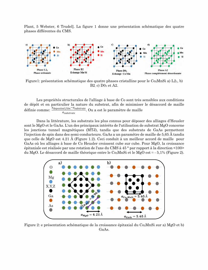
Plant, 5 Webster, 6 Trudel]. La figure 1 donne une présentation schématique des quatre
phases différentes du CMS.
Figure1: présentation schématique des quatre phases cristalline pour le Co2MnSi a) L21, b)
B2, c) D03 et A2.
Les propriétés structurales de l'alliage à base de Co sont très sensibles aux conditions
de dépôt et en particulier la nature du substrat, afin de minimiser le désaccord de maille
définie comme: 𝑎𝑑𝑒𝑝𝑜𝑠𝑖𝑡𝑒𝑑 𝑓𝑖𝑙𝑚−𝑎𝑠𝑢𝑏𝑠𝑡𝑟𝑎𝑡𝑒
𝑎𝑠𝑢𝑏𝑠𝑡𝑟𝑎𝑡𝑒. Ou a est le paramètre de maille
Dans la littérature, les substrats les plus connus pour déposer des alliages d’Heusler
sont le MgO et le GaAs. L'un des principaux intérêts de l'utilisation de substrat MgO concerne
les jonctions tunnel magnétiques (MTJ), tandis que des substrats de GaAs permettent
l'injection de spin dans des semi-conducteurs. GaAs a un paramètre de maille de 5,65 Å tandis
que celle de MgO est 4.21 Å (Figure 1.2). Ceci conduit à un meilleur accord de maille pour
GaAs où les alliages à base de Co Heusler croissent cube sur cube. Pour MgO, la croissance
épitaxiale est réalisée par une rotation de l'axe du CMS à 45 ° par rapport à la direction <100>
du MgO. Le désaccord de maille théorique entre le Co2MnSi et le MgO est ≈ - 5,1% (Figure 2).
Figure 2: e présentation schématique de la croissance épitaxial du Co2MnSi sur a) MgO et b)
GaAs.

Le comportement magnétique de ces alliages dépend fortement de la phase structurale
dans laquelle il croît. Théoriquement Picozzi et al [7 Picozzi] ont montré que dans les phases
L21 et B2, ont une valeur de l'aimantation d’environ 5 μb /f.u. (1,3 T), même lorsque le Mn et
le Si échangent leurs positions dans le réseau pour former la phase B2. Le comportement
demi-métallique du CMS est montré théoriquement avec une “ band gap“ au niveau de fermi
pour la phase L21 avec un faible Gilbert coefficient d'amortissement de 6 * 10-5. Le CMS
présente une anisotropie cubique avec une constante d'anisotropie négative. Ainsi l'axe de
facile aimantation est orienté dans les diagonales du cube (directions <111>) et l'axe de
difficile aimantation est le long des arêtes du cube (directions <100>). Beaucoup d’études ont
été menées sur les phases L21 et B2. Cependant peu d’études ont été menées s sur les phases
de D03 et A2. Théoriquement, Picozzi et al. ont également étudié l'effet de la réorganisation
atomique sur l'aimantation moyenne lorsque en présence d’échange de type Co/Mn (échange
de type D03). Ils ont montré une diminution de l'aimantation à saturation à 4,5 μb /f.u. (1,16
T) mais aucune information sur les variations de l’anisotropie ou du facteur d’amortissement
ne sont donnés. Pour la phase A2 aucune information n'a été trouvée sur le comportement
magnétique de cette phase.
Ainsi l’objectif de ce travail consiste à étudier et comprendre les corrélations entre les
propriétés structurales et magnétiques du CMS à l'échelle atomique. Pour atteindre cet
objectif, nous avons utilisé la technique d'irradiation ionique. Dans ce processus des ions sont
accélérés et pénètrent dans un solide pour modifier les propriétés physiques et chimiques par
interaction nucléaire et électronique. Dans une vision simplifiée, l'irradiation ionique peut
être considérée comme un transfert d’énergie cinétique des ions incidents aux atomes du
réseau. La fluence est définie comme le nombre d’ions / cm2. A faible fluence, l'irradiation agit
comme un recuit local où le transfert d'énergie cinétique conduira à un léger mouvement des
atomes localement pouvant amener une réorganisation chimique locale. Pour les fortes
fluences, l’accumulation d’énergie transmise aux atomes du cristal leur permettra de se
déplacer sur de plus grandes distances et créer des défauts ponctuels de types lacunes ou
interstitielles dans le matériau.
Dans ce travail nous avons utilisé des ions He+ accélérés par une tension de 150 KeV.
Nous avons déterminé les fluences de travail à partir de simulations d’endommagement du
CMS avec le logiciel IPROS développé dans notre laboratoire. Ce logiciel permet de simuler
l’endommagement d’un matériau amorphe et de composition stœchiométrique (50% de Co,
25% de Mn et 25% Si). En plus les simulations sont réalisées à 0K et négligent les potentielles
recombinaisons atomiques à température ambiante. A partir des simulations deux
caractéristiques importantes peuvent être obtenues (figures 3-a et 3-b). La première est
quelles ions parcourent environ 600 nm dans le MgO (dans notre cas 42 nm), Le deuxième
est le nombre de lacunes créées. Par exemple pour une fluence de 1016 ions/cm², nous obtenons
presque 1 lacunes pour 100 atomes de CMS. Cependant, du fait des limitations évoquées ci-
dessus, ce chiffre est surévalué et ne donne qu’une limite haute de l’endommagement possible.
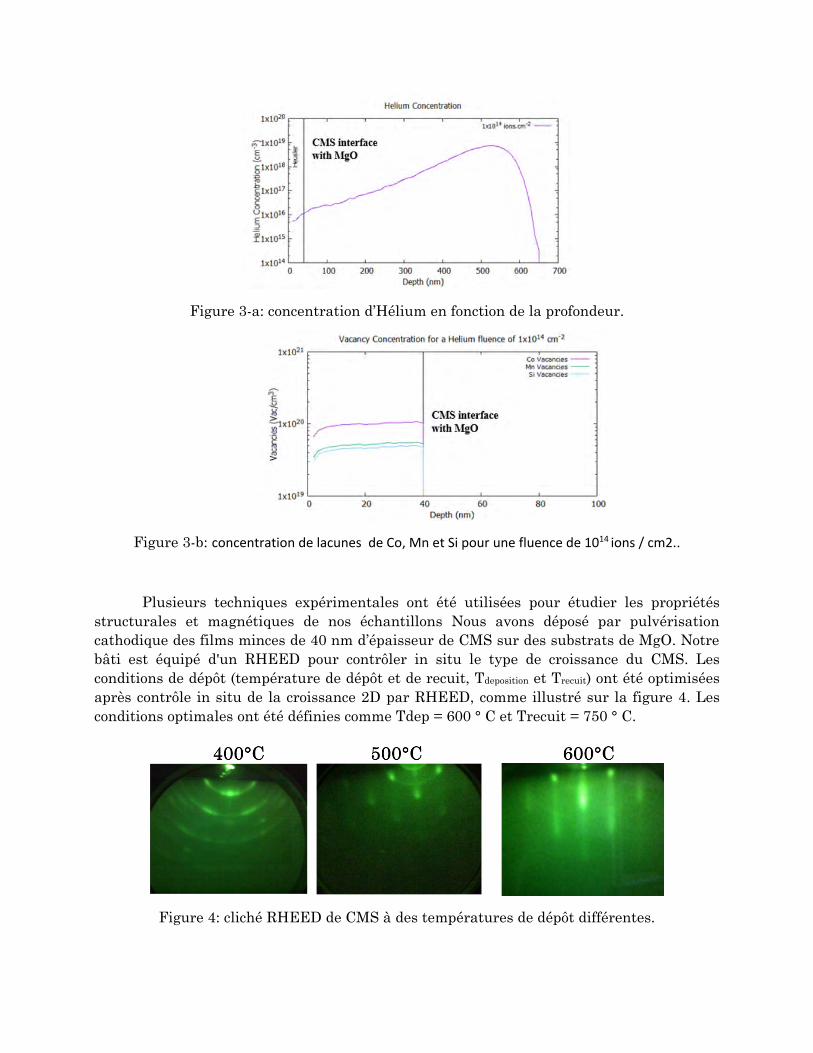
Figure 3-a: concentration d’Hélium en fonction de la profondeur.
Figure 3-b: concentration de lacunes de Co, Mn et Si pour une fluence de 1014 ions / cm2..
Plusieurs techniques expérimentales ont été utilisées pour étudier les propriétés
structurales et magnétiques de nos échantillons Nous avons déposé par pulvérisation
cathodique des films minces de 40 nm d’épaisseur de CMS sur des substrats de MgO. Notre
bâti est équipé d'un RHEED pour contrôler in situ le type de croissance du CMS. Les
conditions de dépôt (température de dépôt et de recuit, Tdeposition et Trecuit) ont été optimisées
après contrôle in situ de la croissance 2D par RHEED, comme illustré sur la figure 4. Les
conditions optimales ont été définies comme Tdep = 600 ° C et Trecuit = 750 ° C.
Figure 4: cliché RHEED de CMS à des températures de dépôt différentes.

L’épaisseur du CMS varie de 40 à 50 nm et à la fin du procédé, une couche de 10 nm de MgO
a été déposée pour empêcher l'oxydation de l'échantillon. Après avoir réalisé l’échantillon, la
diffraction par rayons X et la microscopie électronique en transmission (TEM) sont utilisés
pour étudier la structure et le désordre atomique de nos échantillons. La diffraction de rayons
X est un outil qui permet de caractériser la structure à l'échelle macroscopique. La première
chose que nous avons vérifiée est la relation d’épitaxie du CMS avec le MgO avec une rotation
de la maille du CMS par rapport au MgO. De plus, la diffraction de rayons X permet d’avoir
accès au différents échange atomique et donc aux phases cristallines en présence. En effet,
dans le CMS, certains pics de diffraction apparaissent quel que soit la phase cristalline. On
les appelle les pics fondamentaux (par exemple (220)). Cependant des pics de sur-structure
peuvent apparaitre en fonction du type de désordre présent dans le matériau. Par exemple le
pic de diffraction (111) apparait en présence des ordres cristallins L21 ou D03. Un problème
majeur dans la littérature est que la présence de ce pic de diffraction est généralement
attribuée directement à la présence de la phase L21, ce qui est faux. Ainsi, afin d’avoir accès
à l’ensemble des types de désordre présent dans nos échantillons nous avons suivis l’approche
développé par Niculescu et al. [8 Niculesci] et employé par Takamura [9 Takamura] dans le
cas du Co2FeSi. Dans ce modèle trois paramètres de désordre sont définis 𝛼, 𝛽 et 𝛾. α
corresponds au nombre d’atome de Mn sur les sites de Si par formule unité, β est le nombre
d’atome de Co sur les sites de Si et γ est le nombre d’atomes de Co sur les sites du Mn. Ces
paramètres de désordre sont ensuite introduit dans le calcul des facteurs de structures des
différents plans de diffraction et dans le calcul de l’intensité diffractée tel que :
𝐼ℎ𝑘𝑙 ≈ 𝐿ℎ𝑘𝑙(𝜃)𝑃ℎ𝑘𝑙(𝜃)|𝐹ℎ𝑘𝑙|2 1
sin𝜃ℎ𝑘𝑙 Eq.1
F111 ∝ (1 − 2α − β)(𝑓Mn − 𝑓Si) + (γ − β)(𝑓Co − 𝑓Mn) Eq.2
F002 ∝ (1 − 2β)(𝑓Co − 𝑓Si) + (1 − 2γ)(𝑓Co − 𝑓Mn) Eq.3
F022 = F004 ∝ 2𝑓Co + 𝑓Mn + 𝑓Si Eq.4
Dans cette méthode, trois rapports d’intensités entre les pics de sur-structure hkl et le pic
fondamental doivent être évalués afin d'obtenir 𝛼, 𝛽 et 𝛾.
Afin d'obtenir ces trois paramètres, nous avons utilisé deux diffractomètres, l’un équipé avec
une source de cuivre au seuil Kα et l’un équipé d’une source de cobalt au seuil Kα. L’utilisation
du premier permet d’obtenir α et β car le facteur de diffusion du Co et du Mn à cette énergie
étant très proches (figure 5-a) le second terme du membre de droite des équations 2 et 3
disparaissent. En revanche ces termes réapparaissent au seuil Kα du Co, permettant ainsi de
retrouver le paramètre γ.
Pour étudier l'effet de l'irradiation, l'échantillon déposé a été coupé en 4 morceaux, la
référence et 3 échantillons irradiés à 150 keV de fluences 1015, 5 * 1015 et 1016 ions/cm2,
respectivement.
La figure 6 présente différents pics de diffraction de l’échantillon de référence et des
échantillons irradiés où l'on peut voir clairement le décalage des pics de diffraction vers des
angles plus faibles pour les pics 022, 022 et 004. A partir de ces spectres, on peut d'abord
obtenir le paramètre de maille du CMS. Les valeurs obtenues sont résumées dans le tableau

1. Nous observons que l’irradiation augmente la déformation tétragonale du réseau, tout en
gardant les paramètres dans le plan constant à 5,63 Å. Cette distorsion tétragonale affectera
l'anisotropie magnétique présentée dans la section suivante.
Figure 5: facteurs de diffusion atomique du Co, Mn et Si en fonction of 𝑠𝑖𝑛𝜃ℎ𝑘𝑙
𝜆 pour les
sources de a) Co kα1 et b) Cu kα1.
Figure 6: Diffraction des rayons X . 2𝜽 scan pour l’échantillon de référence et les 3
échantillons irradiés pour les sources de Co et Cu. a), b) et c) représente les 111,002 et 022
pics acquis avec la source de Co. d) et e) présente les pics 002 et 004 acquis avec la source de
Cu.
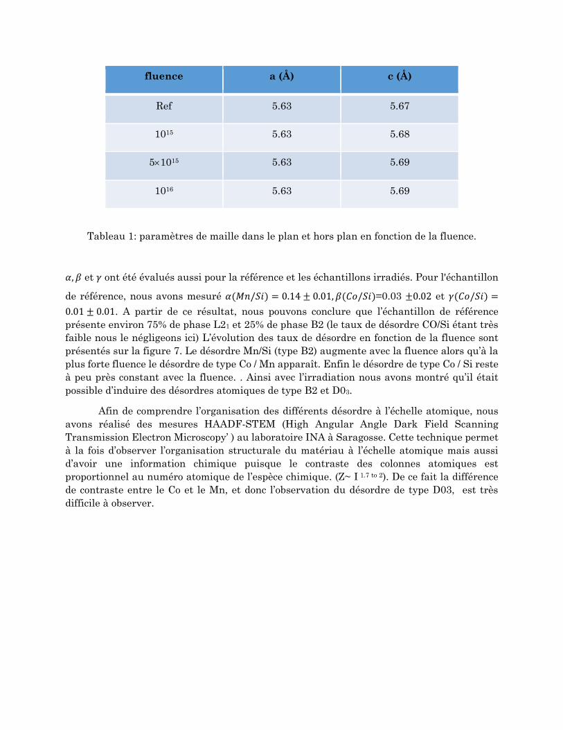
fluence a (Å) c (Å)
Ref 5.63 5.67
1015 5.63 5.68
51015 5.63 5.69
1016 5.63 5.69
Tableau 1: paramètres de maille dans le plan et hors plan en fonction de la fluence.
𝛼, 𝛽 et 𝛾 ont été évalués aussi pour la référence et les échantillons irradiés. Pour l'échantillon
de référence, nous avons mesuré 𝛼(𝑀𝑛/𝑆𝑖) = 0.14 ± 0.01, 𝛽(𝐶𝑜/𝑆𝑖)=0.03 ±0.02 et 𝛾(𝐶𝑜/𝑆𝑖) =
0.01 ± 0.01. A partir de ce résultat, nous pouvons conclure que l’échantillon de référence
présente environ 75% de phase L21 et 25% de phase B2 (le taux de désordre CO/Si étant très
faible nous le négligeons ici) L’évolution des taux de désordre en fonction de la fluence sont
présentés sur la figure 7. Le désordre Mn/Si (type B2) augmente avec la fluence alors qu’à la
plus forte fluence le désordre de type Co / Mn apparaît. Enfin le désordre de type Co / Si reste
à peu près constant avec la fluence. . Ainsi avec l’irradiation nous avons montré qu’il était
possible d’induire des désordres atomiques de type B2 et D03.
Afin de comprendre l’organisation des différents désordre à l’échelle atomique, nous
avons réalisé des mesures HAADF-STEM (High Angular Angle Dark Field Scanning
Transmission Electron Microscopy’ ) au laboratoire INA à Saragosse. Cette technique permet
à la fois d’observer l’organisation structurale du matériau à l’échelle atomique mais aussi
d’avoir une information chimique puisque le contraste des colonnes atomiques est
proportionnel au numéro atomique de l’espèce chimique. (Z~ I 1.7 to 2). De ce fait la différence
de contraste entre le Co et le Mn, et donc l’observation du désordre de type D03, est très
difficile à observer.
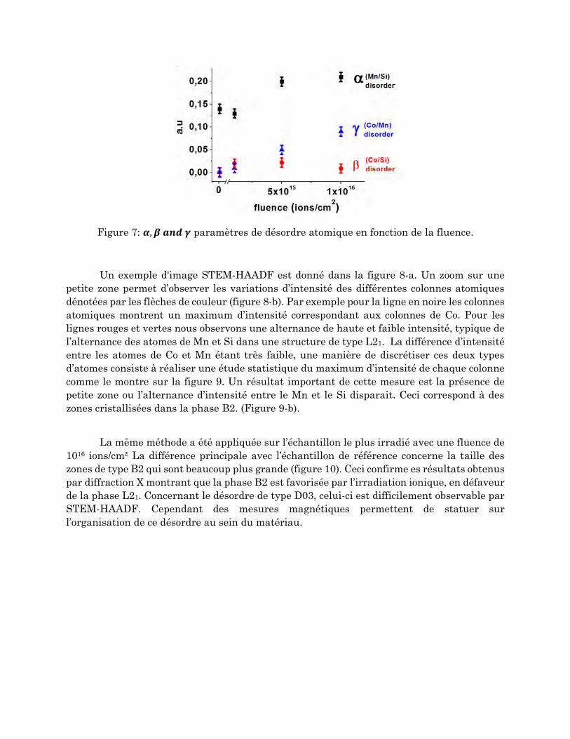
Figure 7: 𝜶, 𝜷 𝒂𝒏𝒅 𝜸 paramètres de désordre atomique en fonction de la fluence.
Un exemple d'image STEM-HAADF est donné dans la figure 8-a. Un zoom sur une
petite zone permet d’observer les variations d’intensité des différentes colonnes atomiques
dénotées par les flèches de couleur (figure 8-b). Par exemple pour la ligne en noire les colonnes
atomiques montrent un maximum d’intensité correspondant aux colonnes de Co. Pour les
lignes rouges et vertes nous observons une alternance de haute et faible intensité, typique de
l’alternance des atomes de Mn et Si dans une structure de type L21. La différence d’intensité
entre les atomes de Co et Mn étant très faible, une manière de discrétiser ces deux types
d’atomes consiste à réaliser une étude statistique du maximum d’intensité de chaque colonne
comme le montre sur la figure 9. Un résultat important de cette mesure est la présence de
petite zone ou l’alternance d’intensité entre le Mn et le Si disparait. Ceci correspond à des
zones cristallisées dans la phase B2. (Figure 9-b).
La même méthode a été appliquée sur l’échantillon le plus irradié avec une fluence de
1016 ions/cm² La différence principale avec l’échantillon de référence concerne la taille des
zones de type B2 qui sont beaucoup plus grande (figure 10). Ceci confirme es résultats obtenus
par diffraction X montrant que la phase B2 est favorisée par l’irradiation ionique, en défaveur
de la phase L21. Concernant le désordre de type D03, celui-ci est difficilement observable par
STEM-HAADF. Cependant des mesures magnétiques permettent de statuer sur
l’organisation de ce désordre au sein du matériau.
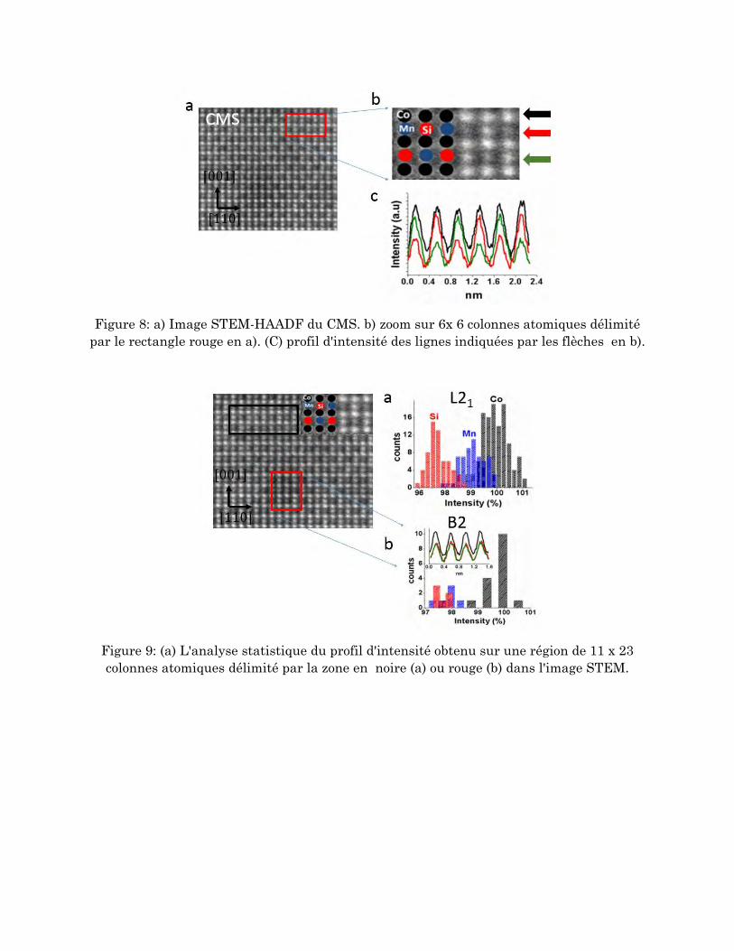
Figure 8: a) Image STEM-HAADF du CMS. b) zoom sur 6x 6 colonnes atomiques délimité
par le rectangle rouge en a). (C) profil d'intensité des lignes indiquées par les flèches en b).
Figure 9: (a) L'analyse statistique du profil d'intensité obtenu sur une région de 11 x 23
colonnes atomiques délimité par la zone en noire (a) ou rouge (b) dans l'image STEM.

Figure 10: Image STEM-HAADF sur l’échantillon irradié à 1016 ions/cm². Les statistiques
ont été effectuées sur les colonnes atomiques délimitées par les zones entourées en a).
La deuxième partie du travail de thèse a consisté à étudier l'effet du désordre atomique
sur les propriétés magnétiques du CMS par résonance ferromagnétique (RFM). La RFM
décrit la précession uniforme de l’aimantation lorsque celle-ci est mise hors de sa position
d’équilibre définie par la direction du champ effectif Heff (qui est défini par la somme des
énergies magnétiques mises en jeu). L’équation du mouvement de l’aimantation est définie
dans l'équation 5. Afin de permette le retour à l’équilibre de l'aimantation, un terme de
relaxation de type frottement visqueux et décrit par le Gilbert facteur d'amortissement 𝛼 est
introduit.
𝒅
𝒅𝒕= −𝜸 𝝁𝟎( ∧ 𝒆𝒇𝒇) +
𝜶
𝑴( ∧
𝒅
𝒅𝒕) Eq.5
Pour étudier les propriétés magnétiques, nous avons développé au CEMES une technique
RFM présentée schématiquement dans la figure 11. Le principe est le suivant. L’échantillon
de CMS est placé au-dessus d’une ligne de transmission micro-ruban constituée d'une couche
d'or de largeur de 400 nm sur un substrat d'alumine.. Une courante micro-onde (0.1 – 30 GHz)
est injectée dans la ligne Afin d’exciter l’aimantation. Le porte objet est placé entre les pôles
d’un électro-aimant pouvant délivrer jusqu’à 1.5 T dans un entrefer de 2 cm ou 0.6 T dans un
entrefer de 8 cm. La mesure consiste à balayer la valeur du champ magnétique extérieur en
gardant une fréquence d’excitation micro-ondes constante. A la résonance, nous mesurons par
une technique de modulation du champ externe la dérivée de la puissance électromagnétique
absorbée par l’échantillon. Cette modulation est réalisée grâce à deux bobines de Helmholtz
placée autour du porte objet. La figure 12 présente un spectre RFM typique qui peut être
mesuré avec notre set-up. Le champ de résonance est définie comme la valeur pour laquelle
le signal est égal à zéro et la largeur de raie ΔHpp définie par la largeur pic à pic dans notre
mesure peut être reliée au facteur de relaxation via la relation ∆𝐻𝑝𝑝 =1
√3∆𝐻, avec ΔH la
valeur FMR réelle.

Figure 11: illustration schématique de la configuration FMR.
Figure 12: Signal FMR mesurée en fonction du champ extérieur appliqué.
Le spectre FMR de l’échantillon de CMS de référence est présenté sur la figure 13.
Deux pics de résonance sont clairement visibles en accord avec la présence des phases B2 et
L21 déterminées par diffraction X et STEM-HAADF. La même chose est observée quel que
soit la direction d’application du champ par rapport aux directions cristallines. Un point
important à prendre en considération est le mélange des modes qui rendent difficile

l’évaluation précise de la largeur de raie dans certaines directions d’application duc champ
extérieur.
En effet, alors que nous pouvons observer clairement deux pics pour l’axe de difficile
aimantation N° 2 (dans le CMS il y a deux axes faciles et deux axes difficiles orientés tous les
45°), on observe un seul pic asymétrique pour l’autre axe difficile N°1. Cependant la forme
asymétrique du pic reflète le fait que les deux modes sont "mélangés". De même, pour l'axe
facile, l'amplitude des deux pics respectifs semble être inversée lorsque le champ extérieur
est appliqué d'un axe facile à l'autre.
Les mesures FMR sont réalisées avec un champ magnétique parallèle ou
perpendiculaire au plan de la couche de CMS. Dans e premier cas, notre montage permet de
tourner le champ magnétique autour de l‘échantillon. Les paramètres magnétiques sont
obtenus à partir des courbes de dispersion fres Vs H0 ou H0 est l’amplitude du champ appliqué.
Pour cela, les données expérimentales (Fres vs. Hres) sont ajustées avec l'équation de Smit-
Belger ; Les paramètres magnétiques obtenus par cette méthode sont résumés dans le tableau
2.
𝝎𝒓𝒆𝒔 =𝜸
𝑴𝒔 𝒔𝒊𝒏𝜽𝒆𝒒[(𝑬𝜽𝜽𝑬𝝋𝝋 − 𝑬𝜽𝝋
𝟐)]𝟏/𝟐 Eq.6
Figure 13: Les spectres d'absorption à 16 GHz en fonction du champ externe à deux axes
durs.

Figure 14: a) relation de dispersion Fres vs. μ0H0 pour l’échantillon de référence pour un
champ appliqué dans le plan de la couche. A droite, zoom sur les deux modes délimitées par
la boîte noire en a).
Figure 15: relation de dispersion pour l'échantillon de référence pour un champ appliqué
perpendiculairement au plan de la couche. b) dépendance angulaire du champ de résonance
à 13 GHz pour un champ appliqué dans le plan de la couche.
Les valeurs de l’aimantation à saturation sont en très bon accord avec la valeur théorique de
la phase L21 (~ 5 μB / f.u) [10 Galanakis]. En nous basant sur les mesures de largeurs de raies
présentées ci-dessous, nous attribuons la phase 1 à l’ordre L21 et la phase 2 à l’ordre B2. Ceci
est en bon accord également avec l’amplitude des pics FMR, plus faible dans le cas de l’ordre
B2 en raison d’un volume plus faible dans l’échantillon. Les valeurs d’aimantation légèrement
plus faible que celles prédites par la théorie peuvent s’expliquer par la présence d’une très
faible quantité de désordre Co/Si comme montré par diffraction X.
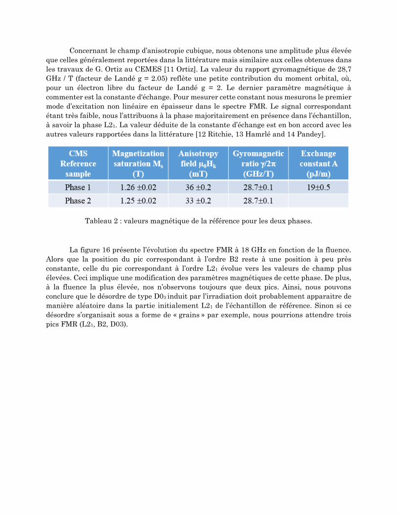
Concernant le champ d’anisotropie cubique, nous obtenons une amplitude plus élevée
que celles généralement reportées dans la littérature mais similaire aux celles obtenues dans
les travaux de G. Ortiz au CEMES [11 Ortiz]. La valeur du rapport gyromagnétique de 28,7
GHz / T (facteur de Landé g = 2.05) reflète une petite contribution du moment orbital, où,
pour un électron libre du facteur de Landé g = 2. Le dernier paramètre magnétique à
commenter est la constante d'échange. Pour mesurer cette constant nous mesurons le premier
mode d’excitation non linéaire en épaisseur dans le spectre FMR. Le signal correspondant
étant très faible, nous l’attribuons à la phase majoritairement en présence dans l’échantillon,
à savoir la phase L21. La valeur déduite de la constante d’échange est en bon accord avec les
autres valeurs rapportées dans la littérature [12 Ritchie, 13 Hamrlé and 14 Pandey].
Tableau 2 : valeurs magnétique de la référence pour les deux phases.
La figure 16 présente l’évolution du spectre FMR à 18 GHz en fonction de la fluence.
Alors que la position du pic correspondant à l’ordre B2 reste à une position à peu près
constante, celle du pic correspondant à l’ordre L21 évolue vers les valeurs de champ plus
élevées. Ceci implique une modification des paramètres magnétiques de cette phase. De plus,
à la fluence la plus élevée, nos n’observons toujours que deux pics. Ainsi, nous pouvons
conclure que le désordre de type D03 induit par l’irradiation doit probablement apparaitre de
manière aléatoire dans la partie initialement L21 de l’échantillon de référence. Sinon si ce
désordre s’organisait sous a forme de « grains » par exemple, nous pourrions attendre trois
pics FMR (L21, B2, D03).

Figure 16: Evolution du spectre FMR à 18 GHz en fonction de la fluence. Le champ
extérieur est appliqué parallèlement à un axe facile.
Figure 17: Evolution des courbes fres vs. μ0H0 pour les deux phases en fonction de la fluence.
Pour la phase B2, les paramètres magnétiques très des courbes de dispersion montrent
que ceux-ci sont constants avec la fluence, excepté une petite augmentation de l’anisotropie
cubique (tableau 3).
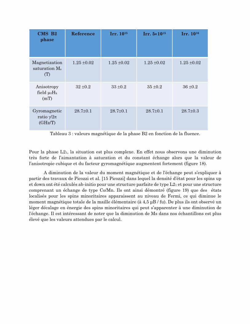
CMS B2
phase
Reference Irr. 1015 Irr. 51015 Irr. 1016
Magnetization
saturation Ms
(T)
1.25 0.02 1.25 0.02 1.25 0.02 1.25 0.02
Anisotropy
field µ0Hk
(mT)
32 0.2 33 0.2 35 0.2 36 0.2
Gyromagnetic
ratio /2
(GHz/T)
28.70.1 28.70.1 28.70.1 28.70.3
Tableau 3 : valeurs magnétique de la phase B2 en fonction de la fluence.
Pour la phase L21, la situation est plus complexe. En effet nous observons une diminution
très forte de l’aimantation à saturation et du constant échange alors que la valeur de
l’anisotropie cubique et du facteur gyromagnétique augmentent fortement (figure 18).
A diminution de la valeur du moment magnétique et de l’échange peut s’expliquer à
partir des travaux de Picozzi et al. [15 Picozzi] dans lequel la densité d’état pour les spins up
et down ont été calculés ab-initio pour une structure parfaite de type L21 et pour une structure
comprenant un échange de type Co/Mn. Ils ont ainsi démontré (figure 19) que des états
localisés pour les spins minoritaires apparaissent au niveau de Fermi, ce qui diminue le
moment magnétique totale de la maille élémentaire (à 4,5 μB / fu). De plus ils ont observé un
léger décalage en énergie des spins minoritaires qui peut s’apparenter à une diminution de
l’échange. Il est intéressant de noter que la diminution de Ms dans nos échantillons est plus
élevé que les valeurs attendues par le calcul.

Figure 18: Evolution de l’aimantation à saturation et de la constante d’échange en fonction
de la fluence.
Figure 19: Densité d’états résolues en spins pour une structure idéale (L21) et une structure
comprenant un désordre de type Co / Mn qui est typique pour l'ordre D03.
Afin d’expliquer l’évolution de l'anisotropie cubique et du rapport gyromagnétique en
fonction de fluence, nous rappelons que ces deux termes dépendent de l’amplitude des
moments magnétiques orbitaux et de spins. En effet le rapport gyromagnétique est liée au
facteur de Landé "g" par la formule suivante:
𝛾 =𝑔∗|𝑒|
2𝑚𝑒 with (𝑔 − 2) = 2
𝜇𝐿
𝜇𝑠
Alors que l'augmentation de l'anisotropie cubique est due à une augmentation éventuelle des
moments orbitaux comme décrit par Bruno et al. [16 Bruno] par cette formule:

∆𝐸𝑆𝑂 = 𝜆[(𝐿. 𝑆)ℎ𝑎𝑟𝑑 − (𝐿. 𝑆)𝑒𝑎𝑠𝑦] =𝜆
4𝜇𝐵(𝜇𝐿
𝑒𝑎𝑠𝑦− 𝜇𝐿
ℎ𝑎𝑟𝑑) > 0
Ainsi, nous pensons que l’augmentation de l’anisotropie cubique et du facteur gyromagnétique
sont probablement lié à l’augmentation du moment magnétique orbital avec le désordre.
Figure 20: Evolution du champ d'anisotropie cubique et du rapport gyromagnétique en
fonction de la fluence
Un autre paramètre magnétique important auquel nous nous sommes intéressés est la
présence d’une faible anisotropie uniaxiale dans le plan des couches. Bien que l’apparition
d’une telle anisotropie est un phénomène connu dans les films minces, son origine physique
est encore débattue. Un mécanisme souvent avancé est un effet de magnéto-mécanique induit
par un effet de contrainte à l’interface avec le substrat. D’autres études proposent que cette
anisotropie provienne de la morphologie du substrat (présence de terrasses par exemple). Des
études GPA menées à partir de l’imagerie STEM-HADDF a montré que nos échantillons sont
parfaitement relaxés et donc l’anisotropie est peut être liée à un effet d’interface avec le
substrat.
Dans l’échantillon de référence celle-ci est alignée avec un axe facile mais nous
observons que son amplitude et la direction évolue sous l’effet de l’irradiation.
La figure 21 présente l'évolution de l'amplitude d'anisotropie uni-axiale μ0Hu et sa direction
par rapport à l’axe de facile aimantation en fonction du paramètre de maille hors plan. La
dépendance quasi linéaire observée laisse penser que l’origine de l’anisotropie réside dans la
déformation intrinsèque de la maille de l’Heusler. Etant donné que les paramètres dans le
plan sont constants il semblerait que la déformation induise une contrainte interne induisant
l’anisotropie. Ceci est confirmé à la plus haute fluence, 1016, pour lequel le matériau est
parfaitement relaxé et pour lequel l'anisotropie disparaît. Nous pensons que ce résultat
obtenu ici sur l’alliage Co2MnSi peut être appliqué à d’autres systèmes ferromagnétiques.

Figure 21: Evolution de l'amplitude de l’anisotropie uni-axiale μ0Hu (a) et de son orientation
par rapport à l’axe facile φu (b) en fonction du paramètre du réseau hors plan.
Enfin la dernière partie de notre étude a porté sur l’étude de la largeur de raie
dynamique en fonction du désordre cristallin.
La largeur de raie dynamique est particulièrement importante d’un point de vue
technologique puisqu’elle représente les pertes d’'énergie. Ceci est particulièrement
important par exemple pour des applications de type guides d’ondes micro-ondes ou pour des
systèmes en spintronique à base de transfert de spins. Théoriquement le coefficient de
relaxation intrinsèque α a été calculé à 0,6*10 -4 . Cependant expérimentalement la valeur la
plus proche récemment rapportée est de 7 * 10-4 [17 Andrieu].
L'évolution de la largeur de raie ΔH pour les pics L21 et B2 dans l’échantillon de
référence sont présentés dans la figure 22. Ici nous ne présentons les résultats que dans le
cas où les deux pics sont bien distincts. La dépendance en fréquence de la largeur de raie est
généralement écrite sous la forme
.∆𝐻= 2 𝜋 𝑓𝛼
𝛾+ ∆𝐻0,
Avec α le coefficient de relaxation de Gilbert (intrinsèque) et ∆𝐻0 les pertes extrinsèques.
Nous observons que la pente, et donc la valeur de α, est la même pour les directions faciles et
difficiles, nous observons une différence de la contribution extrinsèque. Ce résultat n’est pas
clair mais il se peut qu’il soit relié à l’orientation des plans de dislocations dans le MgO
permettant de relaxer le CMS. Nous observons également que la valeur du coefficient de
relaxation est plus faible pour la phase L21 en accord avec les prédictions théoriques. De plus
la valeur obtenue dans la phase L21 est une des meilleures reportées jusqu’ici dans la
littérature.

Fgure 22 : Largeur de raie en fonction de la fréquence pour un champ appliqué le long des
axes faciles et difficiles pour les deux phases observée L21 (gauche) et B2 (droite) pour
l’échantillon de référence.
L’évolution de la largeur de raie pour chaque phase en fonction de la fluence est présentée sur
les figures 23 et 24. Dans le cas de la phase L21 nous observons clairement une augmentation
de α avec la fluence, et donc du désordre. Ici peut s’expliquer par la présence des états de spins
minoritaires calculés par Piccozzi et al. En effet, ces derniers permettent une diffusion inter
bandes avec retournement du spin augmentant ainsi le coefficient de relaxation (dans le
modèle de Kamberski du la relaxation dans les métaux ferromagnétiques [18, 19 Kamberski]).
Pour la phase B2 en revanche nous n’observons pas de variation de α, ce qui est en bon accord
avec l’hypothèse initiale qu’aucun désordre chimique autre que Mn/Si (donc B2) n’apparait
dans les zones de type B2. Cependant nous observons une variation importante des
contributions extrinsèques. A faible fluence celles-ci diminuent. Une explication possible est
l’effet de recuit local apparaissant avec l’irradiation, ce qui peut entrainer une augmentation
du paramètre d’ordre longue portée dans les zones B2 [20 Gaier]. En revanche, à plus forte
fluence les contributions extrinsèques augmentent fortement en raison de la création de
défauts de structure, en accord avec les simulations IPROS.

Figure 23: Evolution avec la fluence de la largeur de raie pour la phase L21 pour un champ
appliqué dans une direction de difficile aimantation.
Figure 24: Evolution avec la fluence de la largeur de raie pour la phase B2 pour un champ
appliqué dans une direction de difficile aimantation.
En conclusion de ce travail:
La caractérisation complète des propriétés du Co2MnSi implique à la fois la caractérisation
structurale et magnétique du matériau.
Intérêt pour la science des matériaux:
• l’échange Mn/Si ne semble avoir aucun impact sur les propriétés magnétiques statiques
mais la valeur du facteur d’amortissement est plus élevée que pour la phase ordonnée L21.

• L’irradiation aux ions He+ favorise la phase B2: cette technique peut ainsi s’avérer
complémentaire des techniques de recuit dans certains procédés industriels
• l’échange Co/Mn affecte considérablement les paramètres magnétiques statiques et
dynamiques, de manière plus importante que ce que des calculs ab-initio laissent prévoir.
Les résultats préliminaires sur l'échange Co/Si semble similaire à l'effet de Co/Mn.
• la déformation tétragonale induit dans le plan une anisotropie uni-axiale. Ceci pose la
question de la validité de notre approche pour d’autres métaux ferromagnétiques.
•Les résultats préliminaires sur la relaxation dynamique:
• Meilleur amortissement observé dans l'ordre L21 (1.5*10-3).
• Amélioration de la largeur de raie pour la phase B2 à faible fluence.
• L’anisotropie de la largeur de raie est démontrée, mais l’anisotropie du coefficient de
relaxation ne peut pas être statuée en l’état
References:
[1] F. Heusler, W. Starck, and E. Haupt, Verh. DPG 5, 220 (1903).”
[2] R. A. De Groot, F. M. Mueller, P. G. Van Engen, et K. H. J. Buschow, « New class of
materials: half-metallic ferromagnets », Phys. Rev. Lett., vol. 50, no 25, p. 2024–2027, 1983.
[3] C. Liu, C. K. A. Mewes, M. Chshiev, T. Mewes, et W. H. Butler, « Origin of low Gilbert
damping in half metals », Appl. Phys. Lett., vol. 95, no 2, p. 022509, 2009.
[4] G. E. Bacon et J. S. Plant, « Chemical ordering in Heusler alloys with the general
formula A2BC or ABC », J. Phys. F Met. Phys., vol. 1, no 4, p. 524, juill. 1971.
[5] P. J. Webster, « Magnetic and chemical order in Heusler alloys containing cobalt and
manganese », J. Phys. Chem. Solids, vol. 32, no 6, p. 1221‑1231, 1971.
[6] S. Trudel, O. Gaier, J. Hamrle, et B. Hillebrands, « Magnetic anisotropy, exchange and
damping in cobalt-based full-Heusler compounds: an experimental review », J. Phys. Appl.
Phys., vol. 43, no 19, p. 193001, mai 2010.

[7] S. Picozzi, A. Continenza, et A. J. Freeman, « Co 2 Mn X ( X = Si , Ge, Sn) Heusler
compounds: An ab initio study of their structural, electronic, and magnetic properties at zero
and elevated pressure », Phys. Rev. B, vol. 66, no 9, sept. 2002.
[8] V. Niculescu, K. Raj, T. J. Burch, et J. I. Budnick, « Correlation of the internal fields,
magnetic moments, and site preferences in Fe 3- x Mn x Si alloys », Phys. Rev. B, vol. 13, no
7, p. 3167, 1976.
[9] Y. Takamura, R. Nakane, et S. Sugahara, « Analysis of L21-ordering in full-Heusler
Co2FeSi alloy thin films formed by rapid thermal annealing », J. Appl. Phys., vol. 105, no 7,
p. 07B109, avr. 2009.
[10] I. Galanakis, P. H. Dederichs, et N. Papanikolaou, « Slater-Pauling behavior and
origin of the half-metallicity of the full-Heusler alloys », Phys. Rev. B, vol. 66, no 17, p. 174429,
nov. 2002.
[11] G. Ortiz Hernandez, « Elaboration et étude des propriétés physiques de couches
minces monocristallines d’alliage de Heusler à faible amortissement magnétique pour
composants hyperfréquences », Université de Toulouse, Université Toulouse III-Paul
Sabatier, 2013.
[12] L. Ritchie, G. Xiao, Y. Ji, T. Y. Chen, C. L. Chien, M. Zhang, J. Chen, Z. Liu, G. Wu, et
X. X. Zhang, « Magnetic, structural, and transport properties of the Heusler alloys Co 2 MnSi
and NiMnSb », Phys. Rev. B, vol. 68, no 10, sept. 2003.
[13] J. Hamrle, O. Gaier, S.-G. Min, B. Hillebrands, Y. Sakuraba, et Y. Ando,
« Determination of exchange constants of Heusler compounds by Brillouin light scattering
spectroscopy: application to Co2MnSi », J. Phys. Appl. Phys., vol. 42, no 8, p. 084005, avr.
2009.
[14] H. Pandey, P. C. Joshi, R. P. Pant, R. Prasad, S. Auluck, et R. C. Budhani, « Evolution
of ferromagnetic and spin-wave resonances with crystalline order in thin films of full-Heusler
alloy Co2MnSi », J. Appl. Phys., vol. 111, no 2, p. 023912, janv. 2012.
[15] S. Picozzi, A. Continenza, et A. Freeman, « Role of structural defects on the half-
metallic character of Co2MnGe and Co2MnSi Heusler alloys », Phys. Rev. B, vol. 69, no 9,
mars 2004.
[16] P. Bruno, « Physical origins and theoretical models of magnetic anisotropy », in
Ferienkurse des Forschungszentrums Julich, 1993.
[17] S. Andrieu, A. Neggache, T. Hauet, T. Devolder, A. Hallal, M. Chshiev, A. M. Bataille,
P. Le Fèvre, et F. Bertran, « Direct evidence for minority spin gap in the
$\mathrmC\mathrmo_2\mathrmMnSi$ Heusler compound », Phys. Rev. B, vol. 93,
no 9, p. 094417, mars 2016.
[18] V. Kamberskỳ, « On ferromagnetic resonance damping in metals », Czechoslov. J.
Phys. B, vol. 26, no 12, p. 1366–1383, 1976.

[19] V. Kamberský, « Spin-orbital Gilbert damping in common magnetic metals », Phys.
Rev. B, vol. 76, no 13, oct. 2007.
[20] O. Gaier, J. Hamrle, S. J. Hermsdoerfer, H. Schultheiß, B. Hillebrands, Y. Sakuraba,
M. Oogane, et Y. Ando, « Influence of the L21 ordering degree on the magnetic properties of
Co2MnSi Heusler films », J. Appl. Phys., vol. 103, no 10, p. 103910, may 2008.