speed control of electrical drives with resonant loadslib.tkk.fi/dipl/2011/urn100498.pdfwaqas ali...
TRANSCRIPT

Waqas Ali
Speed control of electrical drives withresonant loads
School of Electrical Engineering
Master's Thesis submitted in partial ful�llment of the requirement for the degree
of Master of Science in Technology.
Espoo 02.06.2011
Thesis supervisor:
Dr. Marko Hinkkanen
Thesis instructor:
Seppo Saarakkala, M.Sc. (Eng.)
AALTO UNIVERSITY ABSTRACT OF THE
SCHOOL OF ELECTRICAL ENGINEERING MASTER'S THESIS
Author: Waqas Ali
Title: Speed control of electrical drives with resonant loads
Date: 02.06.2011 Language: English Pages: 10 + 56Department of Electrical Engineering
Professorship: Electrical Drives Code: S-81Supervisor: Dr. Marko Hinkkanen
Instructor: Seppo Saarakkala, M.Sc. (Eng.)
This thesis deals with the speed control methods of electrical drives withresonant loads such as rolling mill drives with long shafts, robotic armswith �exible couplings and elevators with �exible ropes. The electricaldrive with a resonant load is modeled as a two-mass resonant system.Three speed controlling techniques have been designed: a state-space con-troller, a two-degree-of-freedom (2DOF) controller tuned according to therigid system model; and a 2DOF controller tuned according to the �ex-ible system model. The state-space controller is designed based on thepole placement technique and with the assumption that all state vari-ables are available. Both 2DOF methods include PI feedback controllers,where two di�erent feedforward controllers are considered. The designprinciples and analytical tuning methods of the controllers are presented.Three simulation studies are carried out to test and analyze the reference-tracking capabilities and sensitivity to disturbances of the designed speedcontrollers. Finally, the bene�ts and limitations of the speed controllersas well as some recommendations for future research areas are presented.
Keywords: Speed control, two-mass resonant system,state-space control, two-degree-of-freedom control,�exible systems, electrical drives.
i
Acknowledgements
The work in this Master's thesis was carried out at Aalto University Schoolof Electrical Engineering under the supervision of Dr. Marko Hinkkanen.
First of all, thanks should be forwarded to God, most gracious, most merci-ful, who guides me in every step I take. I would like to express my deepestgratitude to Professor Jorma Luomi for accepting and giving me this wonder-ful research project, my supervisor Dr. Marko Hinkkanen whose supervisionboth helped me to channel and specify the discussed ideas and at the sametime provided much appreciated freedom and support to explore new waysand concepts. His endless drive for new and better results is highly appre-ciated. I would like to take this opportunity to acknowledge my instructorMr. Seppo Saarakkala, M.Sc. (Eng.) for all his guidance and encouragement.Several ideas in this dissertation have been bene�ted from his insightful dis-cussions. I am very grateful for his endless support, positive and motivatingattitude and for his kind assistance throughout. I also would like to thankMr. William Martin for linguistic editing and proofreading my thesis.
My gratitude to all my friends for their joyous company specially to my friendMr. Muhammad Yasir who has been supportive and motivating for me.
Many thanks to my brother Mr. Shahzad Ali who has been a pillar of supportand comfort during this hard time. Finally, I would like to thank my parentsand whole family, who have always been by my side and provided me withunwavering support throughout my life.
Espoo, 02.06.2011.
Waqas Ali
ii

Abbreviations and symbols
A System matrixB Input matrixC Output matrixCS Shaft damping coe�cientD Feedthrough matrixJL Load inertiaJM Motor inertiaKJ Inertia ratioKR Resonance ratioKS Shaft sti�nesss Laplace variableTL Load torqueTM Motor torqueTS Shaft torqueu Input vectorx State vectorα Angular accelerationαs Bandwidth of 2DOF rigid system modelε Di�erence between motor and load angular positionsζ Damping ratioθL Load angular positionθM Motor angular positionωA Anti resonance frequencyωL Load speedωM Motor speedωR Resonance frequency
iii
Acronyms
PI Proportional-integralPID Proportional-integral-derivative1DOF one-degree-of-freedom2DOF Two-degree-of-freedomMRAC Model reference adaptive control
iv

Contents
Abbreviations and symbols iii
1 Introduction 1
1.1 Background . . . . . . . . . . . . . . . . . . . . . . . . . . . . 1
1.2 Scope . . . . . . . . . . . . . . . . . . . . . . . . . . . . . . . 2
1.3 Objective . . . . . . . . . . . . . . . . . . . . . . . . . . . . . 2
1.4 Disposition . . . . . . . . . . . . . . . . . . . . . . . . . . . . 3
2 Modeling of the two-mass resonant system 4
2.1 Two-mass resonant system . . . . . . . . . . . . . . . . . . . . 4
2.2 State-space representation . . . . . . . . . . . . . . . . . . . . 5
2.3 Transfer function representation . . . . . . . . . . . . . . . . . 7
2.4 System parameters and frequency response . . . . . . . . . . . 8
3 Speed control of two-mass resonant system 12
3.1 Control strategies for the two-mass resonant system . . . . . . 12
3.2 State-space controller design . . . . . . . . . . . . . . . . . . . 17
3.2.1 Control law design for full state feedback . . . . . . . . 17
3.2.2 Integral action . . . . . . . . . . . . . . . . . . . . . . . 21
3.2.3 State-space controller . . . . . . . . . . . . . . . . . . . 22
3.3 Two-degree-of-freedom controller design . . . . . . . . . . . . . 24
3.3.1 Feedback controller . . . . . . . . . . . . . . . . . . . . 24
3.3.2 Feedforward controller . . . . . . . . . . . . . . . . . . 25
v

3.4 2DOF controller for the two-mass resonant system . . . . . . . 28
3.4.1 Parameter tuning according to rigid system model . . . 29
3.4.2 Parameter tuning according to �exible system model . 34
4 Gain calculations and simulations 39
4.1 Introduction to simulation models . . . . . . . . . . . . . . . . 39
4.2 Parameter gain selection . . . . . . . . . . . . . . . . . . . . . 40
4.2.1 Aggressive design of the controllers . . . . . . . . . . . 40
4.2.2 Equivalent rise time for the controllers . . . . . . . . . 44
4.2.3 Equivalent load torque rejection for the controllers . . . 44
4.3 Simulation results . . . . . . . . . . . . . . . . . . . . . . . . . 45
4.3.1 E�ect of encoder model . . . . . . . . . . . . . . . . . . 45
4.3.2 Aggressive design simulation . . . . . . . . . . . . . . . 46
4.3.3 Equivalent rise time simulation . . . . . . . . . . . . . 46
4.3.4 Equivalent load torque rejection simulation . . . . . . . 47
4.4 Performance comparison . . . . . . . . . . . . . . . . . . . . . 52
5 Conclusions 53
vi

List of Tables
2.1 Two-mass resonant system parameters. . . . . . . . . . . . . . 9
3.1 Relationship between the damping behavior and the inertiaratio. (Zhang and Furusho, 2000) . . . . . . . . . . . . . . . . 14
3.2 Comparison of proposed speed control approaches by Thomsenet al. (2010). . . . . . . . . . . . . . . . . . . . . . . . . . . . . 16
4.1 Parameters of dominant and resonant pole pairs. . . . . . . . . 42
4.2 Gain values of the designed controllers for aggressive design. . 43
4.3 Gain values of the designed controllers for the equivalent risetime selection. . . . . . . . . . . . . . . . . . . . . . . . . . . . 44
4.4 Gain values of the designed controllers for the equivalent loadtorque rejection. . . . . . . . . . . . . . . . . . . . . . . . . . . 45
4.5 Measured control performances. . . . . . . . . . . . . . . . . . 52
vii

List of Figures
2.1 Two-mass resonant system. . . . . . . . . . . . . . . . . . . . . 5
2.2 State-space representation as block diagram. . . . . . . . . . . 6
2.3 Block diagram of the two-mass resonant system. . . . . . . . . 8
2.4 Open-loop frequency response from the motor torque to themotor speed. . . . . . . . . . . . . . . . . . . . . . . . . . . . . 10
2.5 Open-loop frequency response from the motor torque to theload speed. . . . . . . . . . . . . . . . . . . . . . . . . . . . . . 11
3.1 System design with control law. . . . . . . . . . . . . . . . . . 18
3.2 Regions of dominant and insigni�cant poles in the s-plane. . . 20
3.3 Integral control structure. . . . . . . . . . . . . . . . . . . . . 22
3.4 State-space controller of the two-mass resonant system withintegral control. . . . . . . . . . . . . . . . . . . . . . . . . . . 23
3.5 Two-degree-of-freedom-control system. . . . . . . . . . . . . . 24
3.6 Conceptual illustration of the control structure's e�ect. . . . . 26
3.7 Detailed block diagram for 2DOF PI control of two-mass res-onant system. . . . . . . . . . . . . . . . . . . . . . . . . . . . 32
3.8 Pole assignment with identical damping coe�cient (Zhang andFurusho, 2000). . . . . . . . . . . . . . . . . . . . . . . . . . . 36
3.9 Overshoot for identical damping coe�cient (Zhang and Fu-rusho, 2000). . . . . . . . . . . . . . . . . . . . . . . . . . . . 37
4.1 Simulation model of the state-space speed control system. . . 40
4.2 Simulation model of the 2DOF speed control system. . . . . . 41
4.3 The e�ect of the encoder model. . . . . . . . . . . . . . . . . . 48
viii

4.4 The step responses of the speed control system for the aggres-sive design. . . . . . . . . . . . . . . . . . . . . . . . . . . . . 49
4.5 The steps response of the speed control system for equivalentrise time. . . . . . . . . . . . . . . . . . . . . . . . . . . . . . . 50
4.6 The steps response of the speed control system for equivalentload torque rejection. . . . . . . . . . . . . . . . . . . . . . . . 51
ix

Chapter 1
Introduction
1.1 Background
In the modern industrial world, motion control (speed, position) is very im-portant to enhance productivity, quality and to reduce energy consumptionas well as equipment maintenance. Its application �elds are widely present inindustry such as pick and place tasks and robotic arms. Electrical drives havea major share in most industrial motion control applications and industrialrobots as these perform the conversion of electrical energy into mechanicalenergy or vice versa in various processes. These drives may operate at con-stant speed or at variable speeds, depending upon the utilizing process, andare considered crucial components in almost all industrial applications.
A signi�cant improvement has been observed in control technology and strate-gies of electrical drives during the last two decades. The technological progressin the industrial world has ampli�ed demand for �exibility and precision aswell as requirement of energy loss minimization due to the global energycrisis. The ease of controlling the electrical drives is an important factor inorder to meet these requirements. This trend owes its progress to the vari-ous philosophies and techniques, developed by several researchers around theworld, such as the PID/PI control scheme, the adaptive control scheme, andthe resonant ratio control scheme.
In many industrial and robotics applications, the mechanical parts of drivesystems may have very low resonant frequency, such as rolling mills whichnormally comprise of a long shaft and large load-side mass, elevators with�exible transmission rope or industrial robotic arms having �exible coupling.A light weight and high load-to-weight ratio construction is required in in-
1

CHAPTER 1. INTRODUCTION 2
dustrial robots for fast motion and high e�ciency in operation. For thesereasons, the dynamics of such systems should be modeled as two-mass ormulti-mass systems. The speed control of such systems has signi�cant in-terest in the scienti�c community due to their importance in the industrialworld. The main tasks of speed controllers are: tracking of the speed ref-erence, rejection the e�ect of load torque and suppression of shaft torsionalvibration.
1.2 Scope
Typical industrial motor drive systems may contain several mechanical cou-plings between a motor and a load. The couplings are not sti�. Thesedrive systems are increasingly required in industrial automation. Howeverthe structural resonance of the drive system is easily excited by rapid changein speed. When �exibility is considered, these drive systems can be modeledas two-mass resonant systems.
A number of strategies have been proposed to design a speed controller forthe two-mass resonant systems. A basic control structure is PI control. Usu-ally, all state variables are not available as well as it is not easy to achieveanalytical design. Also it is hard to develop a uni�ed method to deal withvarious demands. Therefore, it is highly desirable to have an easy-to-tunecontroller which has the ability to control a drive system according to therequirements of the process.
1.3 Objective
The prime objective of this Master's thesis is to design, implement and eval-uate the performance of a two-degree-of-freedom (2DOF) PI speed controllerfor a two-mass resonant system with two di�erent tuning methodologies soas to meet the requirements for typical industrial motor drive systems. Theparameters of the controller will be tuned by following two di�erent method-ologies:
• Parameter tuning according to a rigid system model.
• Parameter tuning according to a �exible system model.
This designing evaluation should be done theoretically and through simula-tion. Since the state-space controller can be considered as the best controller

CHAPTER 1. INTRODUCTION 3
if all state variables are available, we will use it as a benchmark. The per-formance of the 2DOF PI speed controller will be compared with the per-formance of this controller. Hence, it is also required to design a state-spacecontroller while assuming that all state variables can be measured and areavailable for controller design.
The designed 2DOF PI speed controller must possess the following charac-teristics:
• Fast tracking of the load speed with respect to the reference speedwithout overshoot.
• Reject the e�ect of the load torque.
1.4 Disposition
This Master's thesis consists of �ve chapters. The �rst chapter provides abrief introduction of the thesis. Chapter 2 introduces the model of a two-mass resonant system. The prime objective of this thesis begins in Chapter3 where various related control strategies and techniques proposed in thescienti�c community are brie�y reviewed. Then, a state-space controlleris designed and �nally two parameter tuning techniques for the 2DOF PIcontroller are explained for a two-mass resonant system. Chapter 4 containsperformance comparison of the designed controllers based on the simulationresults. Finally, the thesis is concluded in Chapter 5.

Chapter 2
Modeling of the two-mass
resonant system
In this chapter, the structure and the model of a two-mass resonant system isexplained. The block diagram of the system is described followed by a briefreview of the open loop frequency response of the system.
2.1 Two-mass resonant system
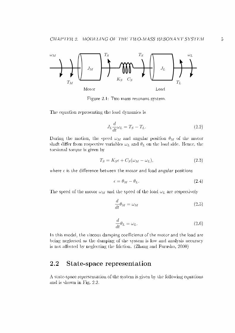
A simple structure of a two-mass resonant system is shown in Fig. 2.1. Thesystem comprises of the motor and the load, connected through a �exibleshaft or transmission element. This �exible shaft or transmission element hasnon-ideal transmission behavior such as �nite torsional sti�ness. This �nitesti�ness can cause unwanted torsional oscillations as well as can stress boththe mechanical and electrical components of the system. The mechanicalparts of such systems may have a low resonant frequency so the structuralresonance is easily excited by rapid change is speed.
Consider a two-mass resonant system where JM is motor inertia, JL is loadinertia, ωM is motor speed, ωL is load speed, TM is motor torque, TL is loadtorque, TS is shaft torque, KS is shaft sti�ness, CS is the shaft dampingcoe�cient, θM is motor angular position and θL is load angular position.(Leonhard, 1996), (Shahgholian et al., 2009b)
The equation representing the motor dynamics is
JMd
dtωM = TM − TS. (2.1)
4
CHAPTER 2. MODELING OF THE TWO-MASS RESONANT SYSTEM 5
Motor Load
ωM ωL
TLTM
JL
TS TS
KS CS
JM
Figure 2.1: Two-mass resonant system.
The equation representing the load dynamics is
JLd
dtωL = TS − TL. (2.2)
During the motion, the speed ωM and angular position θM of the motorshaft di�er from respective variables ωL and θL on the load side. Hence, thetorsional torque is given by
TS = KSε+ CS(ωM − ωL), (2.3)
where ε is the di�erence between the motor and load angular positions
ε = θM − θL. (2.4)
The speed of the motor ωM and the speed of the load ωL are respectively
d
dtθM = ωM (2.5)
d
dtθL = ωL. (2.6)
In this model, the viscous damping coe�cients of the motor and the load arebeing neglected as the damping of the system is low and analysis accuracyis not a�ected by neglecting the friction. (Zhang and Furusho, 2000)
2.2 State-space representation
A state-space representation of the system is given by the following equationsand is shown in Fig. 2.2.

CHAPTER 2. MODELING OF THE TWO-MASS RESONANT SYSTEM 6
Bu
x
x(0)
A
C
Bw
w
u y
Figure 2.2: State-space representation as block diagram.
x = Ax+Buu+Bww (2.7)
y = Cx, (2.8)
where x is the state vector, u is the input vector, A is the system matrix, Bu
and Bw are the input matrices and C is the output matrix. If a system hasn number of states, m number of inputs and r number of outputs then theorders of these matrices are given as: A is n×n matrix, B is n×m matrixand C is r×n matrix. (Buchi, 2010)
The state vector x includes three state variables: the motor speed ωM , theload speed ωL and the di�erence of the angular positions between the motorand the load ε. The control u equals the control input TM and w equals thedisturbance input TL. The output is y. The state-space model of a two-massresonant system is
d
dt
ωMεωL
=
− CS
JM−KS
JM
CS
JM
1 0 −1CS
JL
KS
JL−CS
JL
︸ ︷︷ ︸
A
ωMεωL
︸ ︷︷ ︸
x
+
1JM
00
︸ ︷︷ ︸Bu
[TM]︸ ︷︷ ︸
u
+
00− 1JL
︸ ︷︷ ︸
Bw
[TL]︸︷︷︸
w
(2.9)
y =[0 0 1
]︸ ︷︷ ︸C
ωMεωL
. (2.10)

CHAPTER 2. MODELING OF THE TWO-MASS RESONANT SYSTEM 7
2.3 Transfer function representation
From the state equations, the transfer function of the system can be calcu-lated as
G(s) =Y (s)
U(s)= C(sI−A)−1Bu. (2.11)
A two-mass resonant system can easily be modeled by functional blocks.Considering a two inputs and single output system, the block diagram of thetwo-mass resonant system can be represented as in Fig. 2.3.
Considering (2.11), the open loop transfer function from the motor torque tothe motor speed can be calculated, if we select the matrix C as
C =[1 0 0
], (2.12)
and given in the form
ωM(s)
TM(s)=
1
s(JM + JL)︸ ︷︷ ︸Rigid part
s2JL + sCS +KS
s2 JMJLJM+JL
+ sCS +KS︸ ︷︷ ︸Flexible part
. (2.13)
The transfer function can be assumed to consist of the two parts: the rigidpart and the �exible part. Similarly the open-loop transfer function from themotor torque to the load speed can be calculated, if we select the matrix Cas
C =[0 0 1
], (2.14)
and given as
ωL(s)
TM(s)=
1
s(JM + JL)︸ ︷︷ ︸Rigid part
sCS +KS
s2 JMJLJM+JL
+ sCS +KS︸ ︷︷ ︸Flexible part
. (2.15)
The characteristic equation ∆(s) can be given as
∆(s) = s(s2 + 2ζnωRs+ ωR2). (2.16)

CHAPTER 2. MODELING OF THE TWO-MASS RESONANT SYSTEM 8
ωL(s)1
sJM1sJL
ωM (s)CS
KSs
TS(s)TL(s)
TM (s)
Figure 2.3: Block diagram of the two-mass resonant system.
The resonance frequency ωR and damping ratio ζn are given by
ωR =
√KS
JL(1 +R) , ζn =
CS2
√1
KSJL(1 +R), (2.17)
where R = JL/JM is inertia ratio. The anti-resonance frequency is given as
ωA =
√KS
JL. (2.18)
The anti-resonance frequency is lower than the resonance frequency. Phasecharacteristics of the system change drastically at these frequencies. Exci-tations change with motor-inverter speed, despite the fact that the naturalfrequencies are constant. The resonance characteristics can be explained byits resonance ratio KR which is given
KR =ωRωA
=
√1 +
JLJM
. (2.19)
If we have JM � JL, then the torsional torque oscillations are �ltered by thelarge motor inertia JM and the in�uence of the oscillations on the speed con-trol becomes smaller. In closed-loop motion control, the control bandwidthof the system is limited by the anti-resonance frequency ωA. If the motorinertia JM increases then the resonance frequency ωR decreases, without hav-ing any a�ect on the anti-resonance frequency ωA. On the other hand, bothfrequencies ωR and ωA increase with the increase in the mechanical sti�nessof the shaft KS as well as mechanical bandwidth increases in the closed-loopsystem. (Shahgholian et al., 2009a),(Shahgholian et al., 2009b)
2.4 System parameters and frequency response
In this thesis, we are using the parameters for the two-mass resonant systemgiven in Table 2.1.

CHAPTER 2. MODELING OF THE TWO-MASS RESONANT SYSTEM 9
Table 2.1: Two-mass resonant system parameters.
Parameter Symbol Value Unit
Motor inertia JM 0.0044 kgm2
Load inertia JL 0.0360 kgm2
Shaft sti�ness KS 30 Nm/radShaft damping coe�cient CS 0.05 Nm/rad
An open-loop frequency response from the motor torque to the motor speedcan be obtained by (2.13) and shown in Fig. 2.4, using the system parametersgiven in Table 2.1. The open-loop frequency response from the motor torqueto the load speed by (2.15) is shown in Fig. 2.5.
It can be seen from the frequency response that the system is highly underdamped. From the characteristic equation (2.16), the natural frequenciesand the damping for the poles of system can be calculated. The open-loopsystem has three poles. One pole is in origin where as the resonant pole pairhas the frequency ωR = 87.5 rad/sec and the damping ζ = 0.0729 which is avery small value, indicating that the system is poorly damped.

CHAPTER 2. MODELING OF THE TWO-MASS RESONANT SYSTEM 10
-30
-20
-10
0
10
20
30
Magnitude (
dB
)
100
101
102
103
-90
-45
0
45
90
Phase (
deg)
Bode Diagram
Frequency (rad/sec)
Figure 2.4: Open-loop frequency response from the motor torque to the motorspeed.

CHAPTER 2. MODELING OF THE TWO-MASS RESONANT SYSTEM 11
-80
-60
-40
-20
0
20
40
Magnitude (
dB
)
100
101
102
103
-270
-225
-180
-135
-90
Phase (
deg)
Bode Diagram
Frequency (rad/sec)
Figure 2.5: Open-loop frequency response from the motor torque to the loadspeed.

Chapter 3
Speed control of two-mass
resonant system
In this chapter, �rst a brief literature review of various speed control strate-gies for a two-mass resonant system is presented. After that, a pole place-ment state-space controller design is described. Then, one-degree-of-freedom(1DOF) and 2DOF control designs are discussed. For the 2DOF controllerdesign, a feedforward-type structure is used. Finally, two parameter tuningmethods of the PI-type 2DOF controller are presented.
3.1 Control strategies for the two-mass reso-
nant system
A number of control topologies have been proposed to control the two-massresonant systems. In many industrial and robotics applications, a light weightand high load-to-weight ratio construction is required for fast motion andhigh e�ciency in operation while considering the fact that the mechanicalparts of the drive systems may have a low resonant frequency.
For these reasons, the dynamics of such systems should be modeled as two-mass or multi-mass systems. The speed control of such systems has signi�-cant interest in the scienti�c community due to importance and prevalenceof these systems in the industrial world. The prime objectives of the speedcontrollers are: fast tracking of the speed reference, rejection the e�ect of theload disturbance torque and suppression of the shaft torsional vibration.
Several methods and techniques have been described by researchers to con-
12

CHAPTER 3. SPEED CONTROL OF TWO-MASS RESONANT SYSTEM 13
trol the two-mass resonant system such as using PI/PID controllers, PI-speedcontroller with additional feedback, a state-feedback speed control systemwith and without state observers, an adaptive control scheme, adaptive slid-ing mode neuro-fuzzy control without mechanical sensors and 2DOF con-trollers. A brief description of these control structures is presented here.
Dhaouadi et al. (1993) have presented a scheme of the 2DOF speed controllerfor rolling mills drives. This 2DOF controller uses an observer based state-feedback compensator for major control loop. It is considered that all statevariables are available. They used a set-point �lter type 2DOF structure forspeed controller. Control law design is implemented by the combination ofintegral control compensation and load disturbance feedforward compensa-tion. For state-feedback gain design, the pole-placement technique is used.A roll-o� �lter is used to reduce the system gain beyond the cut-o� frequencyof the system. This speed controller was designed with low overshoot (i.e.10%).
Kim et al. (1996) have described a 2DOF speed control method of the two-mass resonant system, based on the induction machine. For the speed controlof the induction motor, the vector control theory is used. The state observeris constructed from the motor speed which is measured by the speed sen-sor and the torque producing current. This state observer estimates theload speed, the shaft torsional torque and the load disturbance torque. Afeedback controller is designed using these state variables. In order to im-prove the speed response a feedforward controller is also designed by usingthe one-mass system, neglecting the shaft torsional vibration. The completecontrol structure is a 2DOF speed controller. In this controller, the feed-back controller is responsible for the internal stability of the system and thefeedforward controller is designed for fast speed response to the command.This 2DOF controller is compared with the state-feedback controller and it isshown that it is more robust on load disturbance torque and shaft torsionalvibrational as well as contains a fast speed response property.
Hara et al. (1997) provided a comparison for the state feedback-based speedcontrol systems with state observers and without state observers in the mo-tor drives. They have presented a design for a robust state feedback-basedspeed control system considering the stability condition and frequency re-sponse wave shaping. This state-feedback controller is designed by usingonly measureable state variables without a state observer and denoted as apartial state-feedback controller. The optimal feedback gains are determinedby evaluating the appropriate area on the parameter plane, called the gainarea, using Hurwitz stability criterion. Then they have presented a com-

CHAPTER 3. SPEED CONTROL OF TWO-MASS RESONANT SYSTEM 14
Table 3.1: Relationship between the damping behavior and the inertia ratio.(Zhang and Furusho, 2000)
Pole assignment patternInertia ratio
R < 1 1 ≤ R < 2 2 ≤ R ≤ 4 R > 4
Identical radius Under damped Under damped Well damped ImpossibleIdentical damping coe�cient Under damped Under damped Well damped Well damped and over damped
Identical real part Under damped Well damped Well damped Impossible
parison between the state-feedback controller and the partial state-feedbackcontroller by µ analysis. The partial state-feedback controller is not as excel-lent as the state-feedback controller in terms of robust stability when plantparameters are varying but it is easier to apply the partial state-feedbackcontroller due to its simple control system structure without observers.
Zhang and Furusho (2000) have described the redesigning of a conventionalPI speed controller for the two-mass resonant system. The damping char-acteristics of the system are derived and analyzed. They have shown thedependence of the inertia ratio of the load to motor on the dynamic charac-teristics of the system. Three kinds of pole placement techniques have beenused:
• Pole assignment of identical radius.
• Pole assignment of identical damping coe�cient
• Pole assignment of identical real part
The merits of each pole-assignment design are concluded. Finally, a methodis proposed to improve the damping of the system for a small inertia ratioby a derivative feedback of the motor speed. For these three types of poleassignments, the relationship between the damping behavior and the inertiaratio is summarized and shown in Table 3.1 where R = JL/JM is the inertiaratio.
Lee et al. (2006) have described a recursive robust control design methodfor the �exible joints of the industrial robots. These �exible joints can beconsidered as cascade systems composed of two subsystems: the link-sidedynamics and the motor-side dynamics driven by the driving torque input.The controller is designed on the basis of a recursive method for the cascadesystem to achieve the robustness at each step. The robustness of the designedcontroller is compared with the conventional state feedback controller. In thedesign method, they have �rst designed a �ctitious control for the link-side

CHAPTER 3. SPEED CONTROL OF TWO-MASS RESONANT SYSTEM 15
dynamics and then they designed the real control for the overall system sothat the motor-side dynamics e�ectively tracks the �ctitious control. Thereal control part is designed as a PID-controller for the complete system.
A comparative study about vibration suppression in a two-mass resonantsystem from the PI-speed controller and additional feedbacks using the clas-sical pole-placement method is described by Szabat and Kowalska (2007). Inorder to get access to damping, some information is required from the loadside. For a two-mass resonant system, additional feedbacks are required toachieve the desired damping coe�cient and resonant frequency simultane-ously. Rather than using a large number of possible feedbacks, it is shownthat the systems with one additional feedback can be divided into three dif-ferent groups, according to their dynamic characteristics. Finally, a systemwith two additional feedbacks is investigated and then a comparison of theconsidered structures is carried out. The best dynamical characteristics areobtained by the control structure with one additional feedback, from thefollowing possible feedbacks:
• Feedback from derivative of the torsional torque, provided to the torquenode.
• Feedback from the di�erence between the motor and the load speedsprovided to the torque node.
• Feedback from the load speed, provided to the torque node.
Shahgholian et al. (2009a) have presented a PID controller design for the two-mass resonant system by consideration of the frequency response and the stepresponse characteristics. They have used the pole-placement technique whichis based on the coe�cient diagram method to assign the closed-loop poles ofthe system. Then, by using the relation among the coe�cient of the closed-loop characteristic polynomial, the gains of the PID controller are calculated.By comparison, analysis and simulation of the PID controller and the PIDcontroller with active damping, it is shown that a better speed response tosuppress the mechanical vibrations is achieved by using the proposed PIDcontroller tuning.
A state-space analysis and control design for the two-mass resonant systemis presented by Shahgholian et al. (2009b). This methodology depends onthe resonance ratio control by using optimal criterion of the system. Thiscontroller consists of the integral controller and the proportional controllerwith an additional feedback signal from the shaft torque. The controller

CHAPTER 3. SPEED CONTROL OF TWO-MASS RESONANT SYSTEM 16
Table 3.2: Comparison of proposed speed control approaches by Thomsenet al. (2010).
Comparison criteria PISC PI − SSSC GPCSCDynamics
Small-signal performance Low Excellent GoodLarge-signal performance Low Good GoodDisturbance rejection Low Excellent GoodStress of drive shaft High Low LowStability Properties
Relative stability High Excellent MediumRobustness concern, uncertain parameters High High Medium
Calculation time Low Low HighPossibilities of controller design Low High Medium
Complexity of implementation and tuning Low High High
bandwidth in the closed-loop motion control system is limited by the anti-resonant frequency of the system. The controller gains are obtained by thecoe�cient diagram method which is an indirect pole-placement method todesign an appropriate characteristic polynomial.
Thomsen et al. (2010) presented a comparative study of di�erent controlstrategies of the two-mass resonant systems. They describe and comparethree di�erent control methods: the conventional PI control (PISC), the PI-based state-space control (PI−SSSC) and the generalized predictive control(GPCSC). For suitable comparison, the three controller types are designedwith equal bandwidth and veri�ed with the same test setup. The resultsare shown in Table 3.2. The conventional PI-control system provides a lowcontrol performance and high stress on the mechanical system but it is easyto design and implement. More e�ective results are achieved by the GPCSC .The limitation of GPCSC is the required online time calculation. The bestresults are concluded for the PI-based state-space control design due to itsfree pole placement but for this scheme an observer for the estimation of thenon-measured states is required.
Orlowska-Kowalska et al. (2010) has presented a sliding-mode neuro-fuzzyspeed controller, whose connective weights are tuned online according tothe error between the estimated motor speed and the reference model speedfor the two-mass induction motor drives without mechanical sensors. Thee�ectiveness of this adaptive sliding mode neuro-fuzzy speed controller is de-scribed. A gradient descent algorithm is used according to the error between
CHAPTER 3. SPEED CONTROL OF TWO-MASS RESONANT SYSTEM 17
the estimated speed and the reference model output to tune the connectiveweights. The speed of the induction machine is estimated using the modelreference adaptive control (MRAC) scheme and the rotor speed is calculatedon the basis of the error between the measured and the estimated statorcurrents of the motor. It is shown that the proposed controller has betterperformance than the conventional PI controller.
3.2 State-space controller design
In this section, a state-feedback speed controller for a two-mass resonantsystem is designed.
3.2.1 Control law design for full state feedback
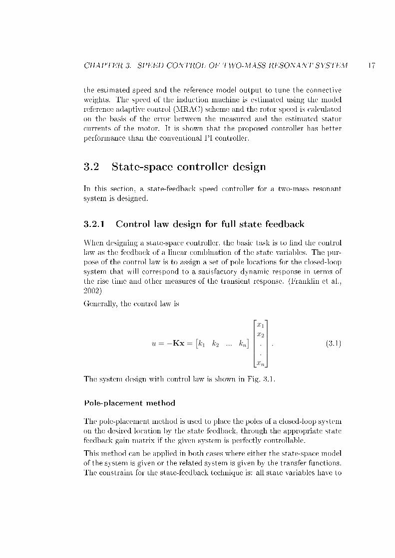
When designing a state-space controller, the basic task is to �nd the controllaw as the feedback of a linear combination of the state variables. The pur-pose of the control law is to assign a set of pole locations for the closed-loopsystem that will correspond to a satisfactory dynamic response in terms ofthe rise time and other measures of the transient response. (Franklin et al.,2002)
Generally, the control law is
u = −Kx =[k1 k2 ... kn
]x1x2..xn
. (3.1)
The system design with control law is shown in Fig. 3.1.
Pole-placement method
The pole-placement method is used to place the poles of a closed-loop systemon the desired location by the state feedback, through the appropriate statefeedback gain matrix if the given system is perfectly controllable.
This method can be applied in both cases where either the state-space modelof the system is given or the related system is given by the transfer functions.The constraint for the state-feedback technique is: all state variables have to
CHAPTER 3. SPEED CONTROL OF TWO-MASS RESONANT SYSTEM 18
uC
y
u = −Kx
Control law
Plant
x = Ax+Buu+Bww
w
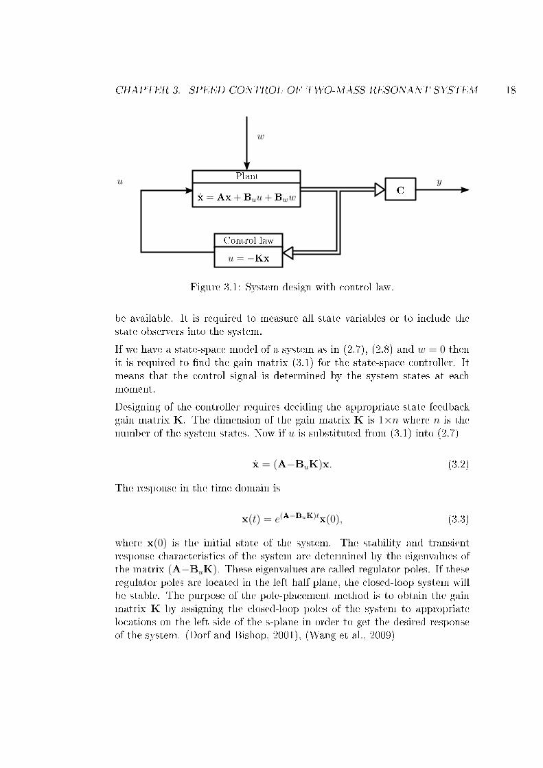
Figure 3.1: System design with control law.
be available. It is required to measure all state variables or to include thestate observers into the system.
If we have a state-space model of a system as in (2.7), (2.8) and w = 0 thenit is required to �nd the gain matrix (3.1) for the state-space controller. Itmeans that the control signal is determined by the system states at eachmoment.
Designing of the controller requires deciding the appropriate state feedbackgain matrix K. The dimension of the gain matrix K is 1×n where n is thenumber of the system states. Now if u is substituted from (3.1) into (2.7)
x = (A−BuK)x. (3.2)
The response in the time domain is
x(t) = e(A−BuK)tx(0), (3.3)
where x(0) is the initial state of the system. The stability and transientresponse characteristics of the system are determined by the eigenvalues ofthe matrix (A−BuK). These eigenvalues are called regulator poles. If theseregulator poles are located in the left half plane, the closed-loop system willbe stable. The purpose of the pole-placement method is to obtain the gainmatrix K by assigning the closed-loop poles of the system to appropriatelocations on the left side of the s-plane in order to get the desired responseof the system. (Dorf and Bishop, 2001), (Wang et al., 2009)

CHAPTER 3. SPEED CONTROL OF TWO-MASS RESONANT SYSTEM 19
Selection of pole locations
An important aspect of the pole-placement design method is to decide, whereto locate the closed-loop poles. The control e�ort required for controlling asystem is related to that how far the open-loop poles are moved by feedback.Furthermore, poles are attracted by open-loop zeros, therefore it is normallyhard to move a pole far away from a nearby zero.
The pole-placement design technique that aims to �x the undesirable aspectsof the open-loop system response will typically allow the smaller controlactuators as compared to that arbitrarily picks all the poles in some locationwithout regard to the original open-loop poles.
There are many techniques to select the appropriate pole locations such as:
• Dominant second-order method.
• Prototype design method.
• Symmetric root locus method.
• Linear quadratic regulator (LQR) method.
The �rst two approaches deal with the pole selection, without explicit regardfor their e�ect on the control e�ort whereas the third technique speci�callyaddresses the issue of achieving a good balanced system response and controle�orts (Franklin et al., 2002). Keeping in mind the open-loop pole locations,the �rst method will be used for designing a state-space controller.
Dominant pole pair design
For a higher order system, closed-loop poles can be considered as a desiredpair of dominant second-order poles; the rest of the poles can be selected tohave real parts corresponding to su�ciently damped modes. In this way, thesystem will mimic a second-order response with reasonable control e�orts.By proper design it is possible to force the closed-loop poles of the higherorder system to the two regions as shown in Fig. 3.2.
A complex conjugate pole pair is placed in Region 1 and all other poles arein Region 2. The pair of complex conjugate pole in Region 1 has a dominante�ect on the transient response of the system and refers as the dominantpole pair of the system. The parameters ζ and ωn of the dominant pole
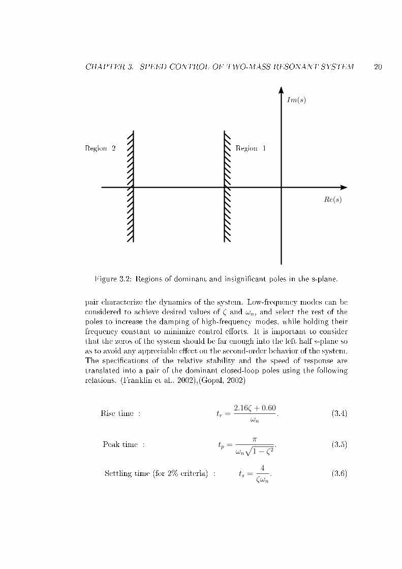
CHAPTER 3. SPEED CONTROL OF TWO-MASS RESONANT SYSTEM 20
Im(s)
Re(s)
Region 1Region 2
Figure 3.2: Regions of dominant and insigni�cant poles in the s-plane.
pair characterize the dynamics of the system. Low-frequency modes can beconsidered to achieve desired values of ζ and ωn, and select the rest of thepoles to increase the damping of high-frequency modes, while holding theirfrequency constant to minimize control e�orts. It is important to considerthat the zeros of the system should be far enough into the left half s-plane soas to avoid any appreciable e�ect on the second-order behavior of the system.The speci�cations of the relative stability and the speed of response aretranslated into a pair of the dominant closed-loop poles using the followingrelations. (Franklin et al., 2002),(Gopal, 2002)
Rise time : tr =2.16ζ + 0.60
ωn. (3.4)
Peak time : tp =π
ωn√
1− ζ2. (3.5)
Settling time (for 2% criteria) : ts =4
ζωn. (3.6)

CHAPTER 3. SPEED CONTROL OF TWO-MASS RESONANT SYSTEM 21
Peak overshoot : Mp = e−πζ/√
1−ζ2 . (3.7)
The desired locations of the closed-loop poles are
s1,2 = −ζωn ± jωn√
1− ζ2. (3.8)
The design requirement is to force two of the closed-loop poles at the speci�eddominant positions and all other poles in the insigni�cant region. A simula-tion study can be performed to see whether the design is acceptable, if not,rearrange the design cycle to get a di�erent distribution of the closed-looppoles. (Franklin et al., 2002),(Gopal, 2002)
3.2.2 Integral action
The state-feedback is a PD-type control. In order to reduce the steady stateerror, integral control is required. Consider a system, having a state-spacemodel as shown in (2.7), (2.8) and w = 0. It is possible to feedback theintegral of the error as well as the states of the plant, while augmenting theplant states with an extra (integral) state xI (Franklin et al., 2002).
This extra integral state obeys the following di�erential equation
xI = Cx− r, (3.9)
where r is the reference input. Hence the integral state xI is
xI =
∫ t
e dt, (3.10)
where e is the error. The augmented state equations for the system become[xIx
]=
[0 C
0 A
] [xIx
]+
[0Bu
]u−
[10
]r. (3.11)
The feedback law is given as
u = −[kI K
] [xIx
]. (3.12)
The block diagram of the system with the integral state xI is represented asin Fig. 3.3.

CHAPTER 3. SPEED CONTROL OF TWO-MASS RESONANT SYSTEM 22
1s
−K
yP lantxI−kI
x
uer
Figure 3.3: Integral control structure.
3.2.3 State-space controller
Considering a two-mass resonant system, a state-space controller is includedin the system to make it a closed-loop system. The block diagram of theclosed-loop system is shown in Fig. 3.4.
The gains can be calculated analytically from the closed-loop model. Thestate-space equations of the closed-loop system are given in (3.11) and (3.12)where kI is the gain for the integral control and the gain matrix K is
K =[k1 k2 k3
], (3.13)
where k1, k2 and k3 are the gains for ωM , ε and ωL, respectively.
The closed-loop system can be presented as[xIx
]=
[0 C
−BukI A−BuK
]︸ ︷︷ ︸
Acl
[xIx
]−[
10
]r. (3.14)
(3.15)
Eigenvalues (poles) of the closed-loop system can be calculated from thecharacteristic equation
B(s) = det(sI−Acl). (3.16)
The characteristics of the closed-loop system can be decided by the pole-placement design method. This closed-loop system with the integral control

CHAPTER 3. SPEED CONTROL OF TWO-MASS RESONANT SYSTEM 23
ωL1sJM
1sJL
ωM CS
KSs
TSTL
TM
k1
k2
k3
1s−kI
u
ωrefL
ControllerTwo−mass resonant system
1s
Figure 3.4: State-space controller of the two-mass resonant system with in-tegral control.
becomes a fourth-order system. The characteristic equation of the system is
B(s) =
Dominant︷ ︸︸ ︷(s2 + 2ζ1ω1 + ω2
1)
Resonant︷ ︸︸ ︷(s2 + 2ζ2ω2 + ω2
2)
=s4 + 2(ζ1ω1 + ζ2ω2)s3 + (ω2
1 + ω22 + 4ζ1ω1ζ2ω2)s
2
+2(ζ1ω1ω22 + ζ2ω2ω
21)s+ ω2
1ω22. (3.17)
ζ1 and ω1 decide the transient response of the system and ζ2 and ω2 areresponsible for the resonance behavior of the system. Comparing (3.16) and(3.17), the following state-feedback gains can be found
kI = −JLJMω21ω
22
KS
(3.18)
k1 =2JLJM(ζ1ω1 + ζ2ω2)− CS(JL + JM)
JL(3.19)
k2 =JLJM(ω2
1 + ω22 + 4ζ1ω1ζ2ω2)− CS(k1 + k3)−KS(JL + JM)
JL(3.20)
k3 =2JLJM(ζ1ω1ω
22 + ζ2ω2ω
21)−KSk1 + CSkI
KS
. (3.21)
It is required to set the values of the tuning parameters ω1, ω2, ζ1 and ζ2 tocalculate the gains for the state-space controller.
CHAPTER 3. SPEED CONTROL OF TWO-MASS RESONANT SYSTEM 24
C(s)yr
Cf (s)
Feedback
Feedforward
Reference input
Manipulated
u
Disturbance
d
P (s)
Controller
PlantControlled variable
controller
controller
variable
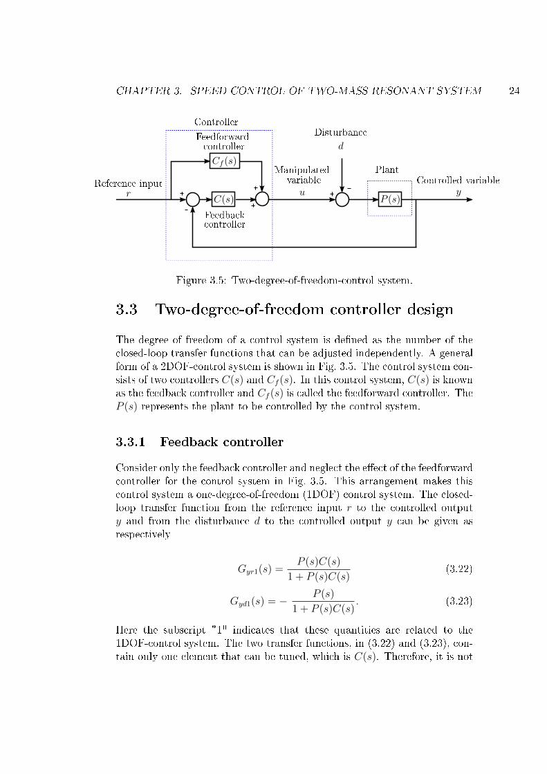
Figure 3.5: Two-degree-of-freedom-control system.
3.3 Two-degree-of-freedom controller design
The degree of freedom of a control system is de�ned as the number of theclosed-loop transfer functions that can be adjusted independently. A generalform of a 2DOF-control system is shown in Fig. 3.5. The control system con-sists of two controllers C(s) and Cf (s). In this control system, C(s) is knownas the feedback controller and Cf (s) is called the feedforward controller. TheP (s) represents the plant to be controlled by the control system.
3.3.1 Feedback controller
Consider only the feedback controller and neglect the e�ect of the feedforwardcontroller for the control system in Fig. 3.5. This arrangement makes thiscontrol system a one-degree-of-freedom (1DOF) control system. The closed-loop transfer function from the reference input r to the controlled outputy and from the disturbance d to the controlled output y can be given asrespectively
Gyr1(s) =P (s)C(s)
1 + P (s)C(s)(3.22)
Gyd1(s) = − P (s)
1 + P (s)C(s). (3.23)
Here the subscript "1" indicates that these quantities are related to the1DOF-control system. The two transfer functions, in (3.22) and (3.23), con-tain only one element that can be tuned, which is C(s). Therefore, it is not

CHAPTER 3. SPEED CONTROL OF TWO-MASS RESONANT SYSTEM 25
possible to change them independently. The relation of these two functionscan be shown as
P (s) = Gyr1(s)P (s)−Gyd1(s). (3.24)
The equation shows that Gyr1(s) can be determined uniquely for any givenP (s), provided Gyd1(s) is chosen and vice versa. Hence, the reference in-put response becomes poor if the disturbance response is optimized and viceversa. Due to this fact, some researchers gave two separate tables for theoptimal tuning of such controllers, where one is for the "disturbance opti-mal" parameters and the other for the "reference input optimal" parameters.(Chien et al., 1952)(R.Kuwata, 1987)
For the 1DOF-control system, it is not possible to optimize the referenceinput response and the disturbance response at the same time. This situationis shown in Fig. 3.6. The bold line indicates the Pareto optimal points forthe 1DOF-control system. Only the hatched area in Fig. 3.6 is realizable bythe 1DOF-control system. Here, points "A" and "B" are de�ned as:
• A is the disturbance optimal point.
• B is the reference input optimal point.
This limitation of the 1DOF-control structure compels to choose from thesealternatives:
1. Choose one of the Pareto optimal points.
2. Use the disturbance optimal parameters and impose limitations on ref-erence input variable change.
The second alternative is very useful for those systems where the referenceinput variable is not changed very often. This limitation can be avoidedby using a 2DOF-control system instead. It provides good means to makeboth the reference input response and the disturbance response practicallyoptimal at once within a linear framework. (Araki and Taguchi, 2003)
3.3.2 Feedforward controller
Consider the complete control system consisting of the feedback controllerand the feedforward controller as shown in Fig. 3.5. This control system is a
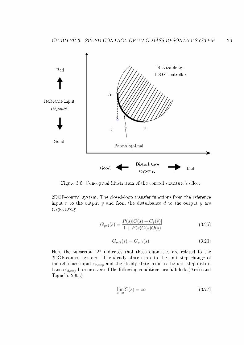
CHAPTER 3. SPEED CONTROL OF TWO-MASS RESONANT SYSTEM 26
A
B
Pareto optimal
Reference input
response
Good
Bad
Disturbance
responseBadGood
C
Realizable by
1DOF controller
Figure 3.6: Conceptual illustration of the control structure's e�ect.
2DOF-control system. The closed-loop transfer functions from the referenceinput r to the output y and from the disturbance d to the output y arerespectively
Gyr2(s) =P (s)[C(s) + Cf (s)]
1 + P (s)C(s)Q(s)(3.25)
Gyd2(s) = Gyd1(s). (3.26)
Here the subscript "2" indicates that these quantities are related to the2DOF-control system. The steady state error to the unit step change ofthe reference input εr,step and the steady state error to the unit step distur-bance εd,step becomes zero if the following conditions are ful�lled: (Araki andTaguchi, 2003)
lims→0
C(s) =∞ (3.27)

CHAPTER 3. SPEED CONTROL OF TWO-MASS RESONANT SYSTEM 27
lims→0
Cf (s)
C(s)= 0 (3.28)
lims→0
P (s) 6= 0. (3.29)
To satisfy these conditions, a simple case is that the C(s) includes an inte-grator but the Cf (s) does not contain any integrator. A number of topologieshave been proposed considering the di�erent industrial aspects for the 2DOF-control system: (Araki and Taguchi, 2003)
• Feedforward-type structure of the 2DOF-control system.
• Feedback-type structure of the 2DOF-control system.
• Set-point-�lter-type structure of the 2DOF-control system.
• Filter and preceded-derivative type structure of the 2DOF-control sys-tem.
• Component separated type structure of the 2DOF-control system.
From all these categories, feedforward-type structure of the 2DOF-controlsystem is of interest to us and it will be used in our design.
The feedforward-type structure of the 2DOF-control system is shown in Fig.3.5. This structure is called feedforward-type due to the presence of a feed-forward path from the reference input r to the manipulated variable u. Thecontroller part is a two-input one-output system. The reference input r andthe controlled output y are the input signals for the controller whereas themanipulated variable u is the output signal of the controller.
Comparing (3.22) and (3.23) with (3.25) and (3.26), it is seen that the closed-loop transfer functions for the 1DOF and the 2DOF-control systems arerelated to each other:
Gyr2(s) = Gyr1(s) +P (s)Cf (s)
1 + P (s)C(s). (3.30)
It can be concluded that

CHAPTER 3. SPEED CONTROL OF TWO-MASS RESONANT SYSTEM 28
• The reference input response of the controllers di�ers by the amountof the second term in (3.30). This term can be changed by adjustingthe Cf (s).
• Both 1DOF and 2DOF-control systems have the same disturbance re-jection response.
Hence, it is expected that from the 2DOF-control system, an improved ref-erence input response can be obtained without deteriorating the disturbanceresponse by appropriate tuning of the Cf (s). For the 2DOF-control system,we can realize point "C" in Fig. 3.6. This clearly shows the advantage of the2DOF-control system over the 1DOF-control system, providing more �exibil-ity and improved results for the 2DOF-control system.(Araki and Taguchi,2003)
3.4 2DOF controller for the two-mass resonant
system
In this section, we will design a 2DOF controller for a two-mass resonantsystem described in Chapter 2. The structure of this 2DOF controller isof the feedforward type, including a feedback controller and a feedforwardcontroller. We will use two di�erent tuning techniques for the parameterselection of the 2DOF controller:
• Parameter tuning according to the rigid system model.
• Parameter tuning according to the �exible system model.
In the �rst tuning method, the two-mass resonant system is considered asa rigid system for the parameter tuning whereas in the second method, the�exible behavior of the two-mass resonant system is also taken into accountfor the parameter tuning.
The primary object in this control system design is to:
• Achieve fast tracking of the load speed with respect to the referencespeed without overshoot.
• Reject the e�ect of the load torque.

CHAPTER 3. SPEED CONTROL OF TWO-MASS RESONANT SYSTEM 29
In order to ensure the stability of the closed-loop system, there must be abandwidth limitation of the feedback loop. It is also required to achieve themaximum possible bandwidth for the 2DOF speed controller. It is importantto notice that in most industrial applications, where it is required to controlthe two-mass resonant system, measured information from the motor side isonly available. The load information is not, usually, available. We will designthe controller by considering the feedback signal from the motor instead ofload, to control the load speed of the system.
3.4.1 Parameter tuning according to rigid system model
The feedforward type structure is used for this 2DOF-control system as shownin Fig. 3.5. In this tuning method we will model and analyze the plant byconsideration of only the rigid part of the two-mass resonant system from(2.13). The �rst step in the design of a 2DOF controller is to design thefeedback controller C(s). The feedback controller C(s) will be a PI controllerwhich provides the stability and satisfactory performance with respect to thedisturbances and the system uncertainties. The second step is to choosethe feedforward controller Cf (s) to shape the overall transfer function of thesystem as well as to obtain the desired command following speci�cations.
Feedback controller design
Consider Fig. 3.5 without taking into account the feedforward controller.The plant P (s) is modeled considering only the rigid part and the feedbackcontroller C(s) is a PI controller. The reference input to the system is thereference load speed ωrefL and the controlled variable is the load speed ωL.
C(s) = KP +KI
s. (3.31)
P (s) =1
s(JM + JL). (3.32)
Considering (3.31) and (3.32), the closed-loop transfer function from ωrefL toωL is given as
ωL(s)
ωrefL (s)=
KP
JM + JL
s+ KI
KP
s2 + ( KP
JM+JL)s+ KI
JM+JL
. (3.33)

CHAPTER 3. SPEED CONTROL OF TWO-MASS RESONANT SYSTEM 30
Similarly, the closed-loop transfer function from TL to ωL is given as
ωL(s)
TL(s)=
−1
JM + JL
s
s2 + ( KP
JM+JL)s+ KI
JM+JL
. (3.34)
The gains are analytically parameterized in terms of the inertia and thedesired closed-loop bandwidth αs. Hence, the values of KP and KI are givenas
KP = αs(JM + JL) (3.35)
KI =
(αs2ζ
)2
(JM + JL). (3.36)
where ζ is the damping coe�cient of the system. Substituting the values ofKP and KI in (3.33) and (3.34), a denominator polynomial for both transferfunctions is obtained as
s2 + αss+
(αs2ζ
)2
. (3.37)
Bandwidth selection
The bandwidth αs should be less than the anti-resonance frequency of thetwo-mass resonant system. Considering the anti-resonance frequency from(2.18), the bandwidth of the system should be selected as
αs ≤√KS
JL. (3.38)
The gains KP and KI of the 2DOF controller can be obtained from (3.35)and (3.36), by appropriate selection of bandwidth αs and damping coe�cientζ of the system.
Feedforward controller design
When the main aim of the speed controlled system is to track the step-alikereference changes, only feedback controller (1DOF control structure) doesnot give su�cient results because of the overshoot. To reduce or eliminate

CHAPTER 3. SPEED CONTROL OF TWO-MASS RESONANT SYSTEM 31
the overshoot appearing in the 1DOF control system, the structure can bemodi�ed by adding a feedforward controller Cf (s) for the reference, to obtainthe 2DOF-control system. The closed-loop transfer functions from the loadspeed reference ωrefL to the load speed ωL becomes
Pc(s) =ωL(s)
ωrefL (s)=Cf (s)P (s) + C(s)P (s)
1 + C(s)P (s). (3.39)
In principle, the closed-loop dynamics can be selected arbitrary by selectinga proper feedforward �lter Cf (s). In this case, tracking of the step-alikereferences is considered which leads to a selection of the �rst-order closed-loop dynamics. Furthermore, let us boost the dynamics of the closed-loopsystem m times. The dynamics of the closed-loop system is to be
Pc(s) =mαs
s+mαs. (3.40)
The transfer function Cf (s) can be solved from (3.39) and (3.40) by substi-tuting the transfer functions of the process P (s) and the PI controller C(s):
Cf (s) =[(JM + JL)mαs −KP ]s−KI
s+mαs. (3.41)
If the PI controller parameters in (3.35) and (3.36) are substituted to (3.41),the transfer function Cf (s) becomes
Cf (s) =(JM + JL)αs[(m− 1)s− αs
4ζ2]
s+mαs. (3.42)
Four special cases can be separated from (3.42):
• If the bandwidth of the 2DOF system is increased compared to the1DOF design (i.e. m > 1), the feedforward �lter Cf (s) is a phase-lead�lter.
• If the bandwidth of the 2DOF system is decreased compared to the1DOF design (i.e. m < 1), the feedforward �lter Cf (s) is a phase-lag�lter.
• If the bandwidth of the 2DOF system is the same as in the 1DOFdesign (i.e. m = 1), the feedforward �lter is simply a low-pass �lter.

CHAPTER 3. SPEED CONTROL OF TWO-MASS RESONANT SYSTEM 32
1sJM
ωM CS
KSs
TS ωL1sJL
TL
Two-mass resonant system
ωrefL
2DOF PI-controller
TMC(s)
Cf (s)
Figure 3.7: Detailed block diagram for 2DOF PI control of two-mass resonantsystem.
• If the bandwidth of the 2DOF system is half of the bandwidth in the1DOF design and the feedback is critically damped (i.e. m = 1/2 andζ = 1), the feedforward �lter is only a constant (Cf (s) = −Jαs/2).This corresponds to the "active-damping" control design. (Harneforset al., 2001)
It is also notable that if the bandwidth of the 2DOF controller is "boosted"(m > 1), the feedforward �lter Cf (s) will have an unstable zero so therewill occur non-minimum phase behavior in the �lter. In this thesis, we areconsidering the third special case and selecting the bandwidth of the 2DOFsystem as m = 1, leading to
Cf (s) = −(JM + JL)(αs
2ζ)2
s+ αs, (3.43)
which is a �rst-order low-pass �lter. The detailed block diagram of the closed-loop system, consisting of the 2DOF controller and the two-mass resonantsystem, is shown in Fig. 3.7.
By parameter selection of the feedforward controller from (3.43) and theparameter selection of the feedback controller from (3.35) and (3.36), the2DOF speed controller can be tuned according to a rigid system model.
Dynamic references tracking
Especially in servo applications, the speed controlled system may not bedriven with the step-alike references. Instead, for example the trapezoidalspeed references are used, when the system is driven from one position toanother. When the trapezoidal velocity reference is used, the speed of the

CHAPTER 3. SPEED CONTROL OF TWO-MASS RESONANT SYSTEM 33
system is �rst accelerated to the constant value and then decelerated backto zero.
Let us study the tracking error of the 1DOF system and the 2DOF systemif the system is accelerated with a constant acceleration α. This means thatthe speed reference is ωrefL (t) = αt, which is in the s-domain ωrefL (s) = α/s2.The tracking error of the closed-loop system Pc(s) can be expressed as
E(s) = ωL(s)− ωrefL (s) = ωrefL (s)[Pc(s)− 1]. (3.44)
Let us solve the steady-state tracking error for both the 1DOF and the 2DOFcontrol structures. The closed-loop TF of the 1DOF control structure is
Pc(s) =αss+ (αs
2ζ)2
s2 + αss+ (αs
2ζ)2. (3.45)
By substituting (3.45) and ωrefL (s) = α/s2 to (3.44), the error becomes
E(s) = − α
s2 + αss+ (αs
2ζ)2. (3.46)
The steady-state tracking error ess can be solved from (3.46) when applyingthe �nal value theorem
ess = limt→∞
e(t) = lims→0
sE(s) = lims→0
(− αs
s2 + αss+ (αs
2ζ)2
)= 0. (3.47)
By substituting (3.40) and ωrefL (s) = α/s2 to (3.44), the error becomes
E(s) = − α
s(s+mαs). (3.48)
Futhermore, the steady-state tracking error ess is
ess = lims→0
(− α
s+mαs
)= − α
mαs. (3.49)
This brief analysis indicates that if the system is desired to follow the dynamicspeed references, one should be careful when using the �rst-order closed-loopmodel. In this simple example, if the acceleration part is long enough, thetracking error of the 2DOF system will approach the value α/(mαs), whenat the same time the tracking error of the 1DOF system will approach tozero.

CHAPTER 3. SPEED CONTROL OF TWO-MASS RESONANT SYSTEM 34
3.4.2 Parameter tuning according to �exible system model
In the tuning method of a 2DOF PI controller presented by Zhang and Fu-rusho (2000), the two-mass resonant system is modeled as the �exible system.It is shown that three kinds of analytical pole placement techniques can beused. The relationship between the damping behavior and the inertia ratiois shown in Table 3.1.
Considering the inertia ratio from the two-mass system parameters presentedin Table 2.1, we get
Inertia ratio : R =JLJM
= 8.18. (3.50)
It is clear from Table 3.1, that only the pole assignment technique "identicaldamping coe�cient" can be applied to this system as the inertia ratio isgreater than 4. We will design the controller using an identical dampingcoe�cient pole assignment technique as described by Zhang and Furusho(2000).
In order to compare both tuning methods, we will rearrange the block di-agram of the control system, presented by Zhang and Furusho (2000) in afeedforward type structure so that we can have a feedback controller C(s) andfeedforward controller Cf (s). In the block digram of the system according toZhang and Furusho (2000), the motor torque is given as
TM(s) =KI
s[ωrefL (s)− ωM(s)]−KPωM(s). (3.51)
Now, if we modify this system so as to use the common PI controller inthe feedback loop and introduce the reference feed-forward �lter, the motortorque is given as
TM =KI
s(ωrefL − ωM) +KP (ωrefL − ωM) + Frω
refL . (3.52)
In order to get same expression for the motor torque, we have to select
Cf (s) = −KP . (3.53)
The modi�ed block diagram for this control system, in terms of the feedfor-ward type structure, is shown in Fig. 3.7.

CHAPTER 3. SPEED CONTROL OF TWO-MASS RESONANT SYSTEM 35
Controller gains
The closed-loop transfer function from the reference input ωrefL to the loadspeed ωL is given as
ωL(s)
ωrefL (s)=
KIωA2
JMs2(s2 + ω2R) + (KP s+KI)(s2 + ω2
A). (3.54)
It is to be noted that this transfer function does not include the shaft dampingcoe�cient CS. Here ωA is anti resonance frequency, ωR is resonance frequencyand R is the inertia ratio of the load to the motor and given as
ωR = ωA√
1 +R. (3.55)
The system in (3.54) can be arranged as
ωL(s)
ωrefL (s)=
ω21ω
22
(s2 + 2ζ1ω1s+ ω21)(s2 + 2ζ2ω2s+ ω2
2), (3.56)
where ω1, ω2 are the natural angular frequencies and ζ1, ζ2 are the dampingcoe�cients. If we compare (3.54) and (3.56), we get following four equations
KP = 2(ζ1ω1 + ζ2ω2)JM (3.57)
KI =ω21ω
22
ω2A
JM (3.58)
ω2A(ω2
1 + ω22 + 4ζ1ζ2ω1ω2)− ω2
1ω22 = ω4
A(R + 1) (3.59)
ω1ζ1(ω22 − ω2
A) = ω2ζ2(ω2A − ω2
1). (3.60)
Since we have only two adjustable feedback coe�cients (Kp, KI), it is notpossible to assign the four poles arbitrarily. From (3.59) and (3.60), we getconstraint relations among the pole locations. The pole locations are directlyrelated to the inertia ratio R of the system as depicted by (3.59).
It is clear from (3.60) that
min(ω1, ω2) ≤ ωA and max(ω1, ω2) ≥ ωA. (3.61)
CHAPTER 3. SPEED CONTROL OF TWO-MASS RESONANT SYSTEM 36
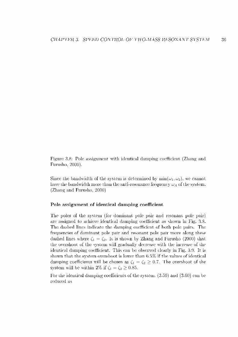
Figure 3.8: Pole assignment with identical damping coe�cient (Zhang andFurusho, 2000).
Since the bandwidth of the system is determined by min(ω1, ω2), we cannothave the bandwidth more than the anti-resonance frequency ωA of the system.(Zhang and Furusho, 2000)
Pole assignment of identical damping coe�cient
The poles of the system (for dominant pole pair and resonant pole pair)are assigned to achieve identical damping coe�cient as shown in Fig. 3.8.The dashed lines indicate the damping coe�cient of both pole pairs. Thefrequencies of dominant pole pair and resonant pole pair move along thesedashed lines where ζ1 = ζ2. It is shown by Zhang and Furusho (2000) thatthe overshoot of the system will gradually decrease with the increase of theidentical damping coe�cient. This can be observed clearly in Fig. 3.9. It isshown that the system overshoot is lower than 6.5% if the values of identicaldamping coe�cients will be chosen as ζ1 = ζ2 ≥ 0.7. The overshoot of thesystem will be within 2% if ζ1 = ζ2 ≥ 0.85.
For the identical damping coe�cients of the system, (3.59) and (3.60) can bereduced as

CHAPTER 3. SPEED CONTROL OF TWO-MASS RESONANT SYSTEM 37
Figure 3.9: Overshoot for identical damping coe�cient (Zhang and Furusho,2000).
(ωAω1
− ω1
ωA
)2
= R− 4ζ21 (3.62)
ω2 =ω2A
ω1
. (3.63)
We can derive ω1 and ω2 from (3.62) and (3.63) and given as
ω1 =
√R− 4ζ21 + 4−
√R− 4ζ21
2ωA (3.64)
ω2 =
√R− 4ζ21 + 4 +
√R− 4ζ21
2ωA. (3.65)
Now ω1 should be a nonnegative real number. Hence, we have to select thevalue of the damping coe�cient as
ζ1 = ζ2 ≤√R
2. (3.66)
If the value of the R is greater than or equal to 4, then the damping coe�cient
values can be assigned within 0 to 1 or (1−√R2
). In this way, the four poles of

CHAPTER 3. SPEED CONTROL OF TWO-MASS RESONANT SYSTEM 38
the system become the two pairs of complex conjugate roots, two double-realroots or four distinct real roots as per the selection of damping coe�cient:
Two pairs of complex conjugate : ζ1 = ζ2 < 1 (3.67)
Two double real roots : ζ1 = ζ2 = 1 (3.68)
Four distinct real roots : ζ1 = ζ2 > 1 (3.69)
From these selections of parameters, the 2DOF controller can be tuned ac-cording to a �exible system model.

Chapter 4
Gain calculations and simulations
In this chapter, the simulation results for the three designed controllers,the state-space (SS) controller, the 2DOF controller with parameter tuningaccording to the rigid system model (2DOFRSM) and the 2DOF controllerwith parameter tuning according to the �exible system model (2DOFFSM)are presented. Finally, the responses of the three controllers are comparedto each other for performance comparison.
4.1 Introduction to simulation models
In this section, the simulation models for the SS-control system and the2DOF-control system are presented. The Matlab/Simulink software is usedfor the modeling and simulation of the speed control system. In the realsystems, the encoders are also present in the complete drive system. Thisencoder, however, will add some noise in the system response. Hence, wehave included an encoder model to incorporate the e�ect of the noise in thesimulation results.
The input to the closed-loop system is the reference load speed ωrefL and theoutput is the load speed response of the system ωL. The load reference speedinput to the closed-loop system is stepped from 0 to 50 rad/sec at 0.1 secondand the load torque is stepped from 0 to 10 Nm at 1.5 second.
In the simulation model, the main blocks of the model are the speed con-troller, the two-mass resonant system and the encoder model. The simula-tion model of the closed-loop system, including the state-space controller, thetwo-mass resonant system and the encoder model is shown in Fig. 4.1. Theclosed-loop system is modeled according to Fig. 3.4. The simulation model
39

CHAPTER 4. GAIN CALCULATIONS AND SIMULATIONS 40
Figure 4.1: Simulation model of the state-space speed control system.
of the speed control system including the 2DOF controller, the two-massresonant system and the encoder model is presented in Fig. 4.2. The speedcontrol system is modeled according to Fig. 3.7.
4.2 Parameter gain selection
The designing rules for the selection of the gains for the controllers are de-scribed in Chapter 3. Considering those gain calculation rules, we will cal-culate the gains of the controllers by using the system parameters given inTable 2.1. First, we will �nd the aggressive design for all controllers to �ndthe maximum bandwidth for each controller. Secondly, the response of theall controllers are examined to achieve the equivalent rise time. Finally, thecontroller parameters are adjusted to achieve the equivalent load torque re-jection.
4.2.1 Aggressive design of the controllers
In order to calculate the gain values for the designed controllers to achievethe maximum bandwidth for 5% overshoot criteria, we are using the designrules as presented in Chapter 3 to calculate the gains for all controllers.
State-space controller's gains
It is clearly evident from (3.17), that the state-space speed control is a fourth-order system. we are considering the dominant pole pair method to select

CHAPTER 4. GAIN CALCULATIONS AND SIMULATIONS 41
Figure 4.2: Simulation model of the 2DOF speed control system.
the frequencies and the damping ratios of the dominant and the resonantpole pairs. Considering that, the parameters ζ1 and ω1 are associated withthe dominant pole pair and the parameters ζ2 and ω2 are associated with theresonant pole pair and represented as
Dominant pole pair : s2 + 2ζ1ω1 + ω12 (4.1)
Resonant pole pair : s2 + 2ζ2ω2 + ω22 (4.2)
The frequency of the resonant pole pair is selected equal to the undampednatural frequency of the system
ω2 = ωR = 87.5 rad/s. (4.3)
Several simulations have been carried out, using di�erent values of the damp-ing ratios ζ1 for the dominant pole pair, ζ2 for the resonant pole pair and themaximum bandwidth of the system to analyze the behavior of the controlsystem. The system response is well damped and has 5% overshoot for thevalues of the damping ratios and the frequencies as shown in Table 4.1.
Ideally, the overshoot can be reduced by increasing the value for the dampingratio of the resonant pole pair ζ2 but in order to compare the response ofthe three designed controllers we have chosen the value of ζ2 to get theovershoot in the system response. It is important to notice that, by selectinga small value of ζ2 for the resonant pole pair, the gain values of the controllerare not too high. It is in favor of good controller design to not select thehigh controller gains as the noise will be ampli�ed by the high gains of thecontroller. For these gain selections, the maximum bandwidth ω1 of thestate-space controller of the two-mass resonant system is 73 rad/sec with 5%

CHAPTER 4. GAIN CALCULATIONS AND SIMULATIONS 42
Table 4.1: Parameters of dominant and resonant pole pairs.
Parameter Dominant pole pair Resonant pole pairζ1 1 -ζ2 - 0.2ω1 73 -ω2 - 87.5
overshoot in the response. The gains for the state-space controller can becalculated by (3.18), (3.19), (3.20) and (3.21), considering the parameters ofthe dominant and the resonant pole pairs and the parameters of the systemin Table 2.1.
2DOF controller's gains according to rigid system model
The gain calculation of the 2DOFRSM controller depends on the bandwidthαs and the damping coe�cient ζ of the system whereas the bandwidth of thecontroller should be less than the anti-resonance frequency of the system.Several simulations have been carried out for the di�erent values of αs andζ to analyze the behavior of the control system. The system response is welldamped and within the required limits of 5% overshoot if the parameters areselected as
αs = 19 rad/sec (4.4)
ζ = 1. (4.5)
For these selections, the gains KP , KI of the controller can be calculatedaccording to (3.35) and (3.36). The low-pass �lter can be designed accordingto (3.43).
2DOF controller's gains according to �exible system model
The parameter selection of the 2DOFFSM controller depends on the naturalangular frequencies and the damping coe�cients. The bandwidth of thesystem is determined by min(ω1, ω2). The bandwidth should be less than theanti-resonance frequency of the system. The natural frequencies ω1 and ω2

CHAPTER 4. GAIN CALCULATIONS AND SIMULATIONS 43
Table 4.2: Gain values of the designed controllers for aggressive design.
GainsSpeed controller type
2DOFRSM 2DOFFSM SS
KP 0.76 0.75 −KI 3.64 6.07 215.42Kf 4.75 − −k1 − − 0.74k2 − − 35.88k3 − − 6.50
Bandwidth 19 11.76 73
are dependent on the damping coe�cients of the system and these can becalculated by (3.64) and (3.65).
Using di�erent damping coe�cient values, several simulations for the controlsystem have been performed to analyze the behavior of the system. Thesystem response is well damped and within the required limits if we choosethe values of damping coe�cients as
ζ1 = ζ2 = 1. (4.6)
By this selection of damping coe�cients, the values of ω1 and ω2 are givenas
ω1 = 11.76 rad/sec (4.7)
ω2 = 70.80 rad/sec. (4.8)
The gains KP , KI of the 2DOF controller, according to �exible system modeltuning, can be calculated by (3.57), and (3.58). The bandwidth of the sys-tem is determined by min(ω1, ω2) so ω1 is the maximum bandwidth of thesystem with 5% overshoot criteria. From the design rules and the parameterselections, the gain values of the three designed controllers are calculated andpresented in Table 4.2.

CHAPTER 4. GAIN CALCULATIONS AND SIMULATIONS 44
Table 4.3: Gain values of the designed controllers for the equivalent rise timeselection.
GainsSpeed controller type
2DOFRSM 2DOFFSM SS
KP 0.25 0.73 −KI 0.38 3.67 4.98Kf 1.54 − −k1 − − 0.19k2 − − 2.69k3 − − 0.73
Bandwidth 6.15 11.76 11.1
4.2.2 Equivalent rise time for the controllers
In order to compare the rise time of all three controllers, the rise time isde�ned as "time taken for the output to rise from 0% to 90% of its �nalvalue when stimulated by a step input".
A number of simulations are done by changing the values of the bandwidthfor the state-space controller and the 2DOFRSM controller to obtain theequal rise time for all the controllers. The equivalent rise time is obtainedif the bandwidth of the state-space controller is selected 11.1 rad/sec andthe bandwidth of the 2DOFRSM controller is selected 6.15 rad/sec. Theremaining parameters of the controllers are selected similarly as in previoussimulation. The equivalent rise time for all the controllers is 0.361 seconds.The gain values of the three designed controllers are calculated and presentedin Table 4.3 for the equivalent rise time selection.
4.2.3 Equivalent load torque rejection for the controllers
The parameters of the 2DOFFSM controller are adjusted similarly. The pa-rameters of the state-space controller and the 2DOFRSM controller will beselected to get the same load torque rejection according to the 2DOFFSMcontroller.
Varying the di�erent values of bandwidth of the controllers, several simula-tions are carried out to acquire the same load torque rejection. For the state-space controller, the damping coe�cient value is also adjusted in addition tothe bandwidth of the controller. All controllers have almost the same load

CHAPTER 4. GAIN CALCULATIONS AND SIMULATIONS 45
Table 4.4: Gain values of the designed controllers for the equivalent loadtorque rejection.
GainsSpeed controller type
2DOFRSM 2DOFFSM SS
KP 0.75 0.75 −KI 3.65 3.65 3.27Kf 4.75 − −k1 − − 0.16k2 − − 0.44k3 − − 1.76
Bandwidth 19 11.76 9
torque rejection if the bandwidth of the 2DOFRSM controller is chosen 19rad/sec and the bandwidth of the state-space controller is selected 9 rad/secwith the damping coe�cient value of the dominant pole pair chosen as 0.8.The remaining parameters of the controllers are selected similarly as in theprevious simulation. The gain values of the three designed controllers arecalculated and presented in Table 4.4 for the equivalent load torque rejectionfor the controllers.
4.3 Simulation results
The simulations are performed for the state-space controller, the 2DOFRSMcontroller and the 2DOFFSM controller using the gain values discussed inthe previous subsections. In these simulations, the actual speed signals areshown.
4.3.1 E�ect of encoder model
In the simulation models of the controllers, an incremental encoder is modeledand added in the closed-loop system. The purpose of the encoder is to addthe noise e�ect in the system response. The comparison in the responses ofthe speed control system for the 2DOFFSM controller is shown in Fig. 4.3with noise and without noise due to the encoder model.

CHAPTER 4. GAIN CALCULATIONS AND SIMULATIONS 46
4.3.2 Aggressive design simulation
The gains of the all three controller are selected according to Table 4.2. Thestep response of the speed control system for each controller is shown in Fig.4.4. This simulation is done for 5% overshoot criteria. In this case, ourinterest is to analyze the capability of the controllers to follow the referencesignal e�ciently. It is clearly visible from the simulation result that the state-space controller is fast as well as has the best load torque rejection amongall the three controllers but there are some transients in the response ofthe system. The reason for these transients is that we are operating near theresonance area. The response of the 2DOFRSM controller is fast as comparedto the response of the 2DOFFSM controller.
The load torque rejection is a little faster in the case of the 2DOF controllertuned according to the �exible system model as compared to the rigid sys-tem model tuning but it also has some overshoot after the recovery in theresponse. In case of rigid system model tuning, the load torque is slightlyslower but it is well damped. In the motor torque TM , maximum noise andmaximum peak value of the torque is observed for the state-space controller.The reason for this noise is the fast response of the state-space controller.The 2DOFFSM controller and the 2DOFRSM controller have almost the sameamount of noise but the latter has a high peak in the motor torque.
In the aggressive design simulation, the 2DOFRSM controller han an edge ofbeing fast in reference following as compared to the 2DOFFSM controller.Both controllers have almost similar load torque rejection but the 2DOFRSMcontroller has a high peak in the motor torque TM .
4.3.3 Equivalent rise time simulation
The controller gains are selected as per Table 4.3. The step response of allthree controllers is shown in Fig. 4.5. In this simulation, the rise time for allthree control designs is �xed.
For equivalent rise time selection, no overshoot is observed in all three con-trollers. The noise in the motor torque is lowest for the 2DOFRSM controllerbut it has very poor load torque rejection. The lowest noise is due to thesmall gain values of the controller. It also has the maximum peak in the mo-tor torque TM . On the other hand, the 2DOFFSM controller has relativelyhigh noise but the load torque rejection is good. The state-space controllerhas the highest noise of all three controller but it has the best load torquerejection.
CHAPTER 4. GAIN CALCULATIONS AND SIMULATIONS 47
In the equivalent rise time simulation, the 2DOFFSM controller has signif-icantly better results as compared to the 2DOFRSM controller. There is asigni�cant di�erence in the load torque rejection of both tuning techniques.In this case, one can easily conclude to prefer the 2DOFFSM controller overthe 2DOFRSM controller.
4.3.4 Equivalent load torque rejection simulation
In order to get the equivalent load torque rejection for all the controllers,the gains are selected according to Table 4.4. The step response of all threecontrollers is shown in Fig. 4.6. It can clearly be observed from the simu-lation results that there is 4.4% overshoot in the response of the 2DOFRSMcontroller and 1.2% overshoot in the response of the state-space controllerfor the same load torque rejection but there is no overshoot in the 2DOFRSMcontroller response. The rise time of the 2DOFRSM controller is the best ofall the controllers but it has the maximum peak in the motor torque TM .The noise is almost the same in response of all controllers.
In the equivalent load torque rejection (Tlr) simulation, the 2DOFFSM con-troller shows better performance than the 2DOFRSM controller. There is noovershoot in response as well as a low peak is observed in the motor torquefor the 2DOFFSM controller.

CHAPTER 4. GAIN CALCULATIONS AND SIMULATIONS 48
0 0.5 1 1.5 2 2.5 3-10
0
10
20
30
40
50
60
Time (s)
ve
locity (
rad
/se
c)
Effect of encoder model
Measured signalActual signal
Figure 4.3: The e�ect of the encoder model.

CHAPTER 4. GAIN CALCULATIONS AND SIMULATIONS 49
0 0.5 1 1.5 2 2.5 3-10
0
10
20
30
40
50
60
Time (s)
ve
locity (
rad
/se
c)
Step response for agressive design
ReferenceSS controller2DOFRSM controller
2DOFFSM controller
5% Over shoot
0 0.5 1 1.5 2 2.5 3-30
-20
-10
0
10
20
30
40
50
60
Time (s)
Mo
tor
torq
ue
(N
m)
SS controller2DOFRSM controller
2DOFFSM controller
Figure 4.4: The step responses of the speed control system for the aggressivedesign.

CHAPTER 4. GAIN CALCULATIONS AND SIMULATIONS 50
0 0.5 1 1.5 2 2.5 3-10
0
10
20
30
40
50
60
Time (s)
ve
locity (
rad
/se
c)
Step response for equivalent rise time
ReferenceSS controller2DOFRSM controller
2DOFFSM controller
90% of final value
0 0.5 1 1.5 2 2.5 3-5
0
5
10
15
Time (s)
Mo
tor
torq
ue
(N
m)
SS controller2DOFRSM controller
2DOFFSM controller
Figure 4.5: The steps response of the speed control system for equivalent risetime.

CHAPTER 4. GAIN CALCULATIONS AND SIMULATIONS 51
0 0.5 1 1.5 2 2.5 3-10
0
10
20
30
40
50
60
Time (s)
ve
locity (
rad
/se
c)
Step response for equivalent load torque rejection
ReferenceSS controller2DOFRSM controller
2DOFFSM controller
0 0.5 1 1.5 2 2.5 3-5
0
5
10
15
20
25
30
35
40
Time (s)
Mo
tor
torq
ue
(N
m)
SS controller2DOFRSM controller
2DOFFSM controller
Figure 4.6: The steps response of the speed control system for equivalentload torque rejection.

CHAPTER 4. GAIN CALCULATIONS AND SIMULATIONS 52
Table 4.5: Measured control performances.Performance Controller Agressive Equivalent Equivalent
parameters design rise time Tlr
Tr (sec)SS 0.044 0.361 0.337
2DOFRSM 0.097 0.361 0.0972DOFFSM 0.214 0.361 0.360
PO (%)SS 5 − 1.2
2DOFRSM 5 − 4.42DOFFSM 5 − −
Tlr
SS best best Good2DOFRSM Good Poor Good2DOFFSM Good Good Good
4.4 Performance comparison
The simulation results are presented in Fig. 4.4, Fig. 4.5 and Fig. 4.6. Theachieved control performances are characterized by the percentage overshoot(PO) in the response of the controllers, the rise time (Tr) and the load torquerejection (Tlr) of the controllers. The values of these performance parametersare summarized in Table 4.5 for each speed controller. The load torquerejection (Tlr) is characterized as best, good and poor considering best as theexcellent and poor as the worst.

Chapter 5
Conclusions
The objective of this Master's thesis was to compare three speed controllingtechniques for the two-mass resonant system: the state-space control, the2DOF control tuned according to a rigid system model and the 2DOF con-trol tuned according to a �exible system model. The control methods weredesigned and compared in terms of their dynamic behavior, reference follow-ing capability and load torque rejection. Furthermore, the e�ect of noise inthe motor torque due to the encoder was also taken into account for eachcontrolling technique.
The state-space controller is designed using the pole placement technique andanalytical calculations are presented for the gains calculation. The feedfor-ward type of 2DOF controller is �rst tuned considering the two-mass resonantsystem as a rigid system and then it is tuned according to a �exible systemmodel. Analytical gain calculations for both tuning techniques are presented.Finally, three simulation studies are used to compare the performance of thedesigned speed controllers: the aggressive design simulation, the equivalentrise time simulation and the equivalent load torque rejection simulation.
It is observed that the best control performance can be achieved by the state-space controller due to its free pole placement property but it is requiredthat all state variables should be available. Usually all state variables arenot available and this condition will limit the performance of the state-spacecontroller.
In the aggressive design simulation, the 2DOFRSM controller has a fasterreference following than the 2DOFFSM controller for almost the same loadtorque rejection. It can be concluded that for the system where the fastrise time is required, the 2DOFRSM controller will be preferred over the2DOFFSM controller but it is to be noted that there is a peak in the motor
53

CHAPTER 5. CONCLUSIONS 54
torque for the 2DOFRSM controller.
In the equivalent rise time simulation, the 2DOFFSM controller had de�-nitely better load torque rejection. The 2DOFRSM controller has poor loadtorque rejection. Both tuning techniques have almost the same peak in mo-tor torque but the �exible system model tuning has much more noise thanthe rigid system tuning. In this case the 2DOFFSM controller shows betterperformances.
In the equivalent load torque rejection simulation, there is overshoot in theresponse of the 2DOFRSM controller as well as a high peak in the motortorque but no overshoot is observed in the 2DOFFSM controller's response.Hence, in this comparison, the 2DOFFSM controller has a clear edge overthe 2DOFRSM controller.
The comparison of all three controllers with pros and cons is presented andthe user has to decide, depending on the required control performance and theavailable control hardware, which of the control method is the most conve-nient one for their system. If future investigations in the area of the two-massresonant system speed control are conducted, the study should concentrateon what the e�ect of state observers is on the state-space controller perfor-mance. For all controller tuning techniques, the robustness of the controllersto parameter variation can be analyzed. Further, it would be interesting tostudy the dynamical reference tracking capability of the controllers.
Bibliography
Araki, M. and Taguchi, H. (2003). Two degree of freedom PID controllers.Proc. Inernational Journal of Control Automation and Systems, 1(4):401�411.
Buchi, R. (2010). State Space Control, LQR and Observer: Step by StepIntroduction, with Matlab Examples. Books on Demand GmbH, Hamberg,Germany, 1st edition.
Chien, K., Hrones, J. A., and Reswick, J. B. (1952). On the automatic controlof generalized passive systems. Trans. ASME, 74:175�185.
Dhaouadi, R., Kubo, K., and Tobise, M. (1993). Two-degree-of-freedomrobust speed controller for high-performance rolling mill drives. IEEETransaction on Industry Applications, 29(5):919�923.
Dorf, R. C. and Bishop, R. H. (2001). Modern Control Systems. PrenticeHall, New Jersey, 9th edition.
Franklin, G. F., Powell, J. D., and Emami-Naeini, A. (2002). Feedback Con-trol of Dynamic Systems. Prentice Hall, New Jersey, 4th edition.
Gopal, M. (2002). Control Systems. Tata McGraw-Hill, Delhi, India, 3rdedition.
Hara, K., Hashimoto, S., Funato, H., and Kamiyama, K. (1997). Robustcomparison between state feedback-based speed control systems with andwithout state observers in resonant motor drives. In International Con-ference on Power Electronics and Drives System, IEEE, volume 1, pages371�376.
Harnefors, L., Pietilainen, K., and Gertmar, L. (2001). Torque-maximizing�eld-weakening control: design, analysis, and parameter selection. Indus-trial Electronics, IEEE Transactions on, 48(1):161�168.
55

BIBLIOGRAPHY 56
Kim, Y.-S., Kim, S.-B., Kim, J.-S., Yoo, C.-H., and Kim, H.-J. (1996). Two-degree-of-freedom speed control of induction motor having two-mass res-onant system. In Industrial Electronics, Control, and Instrumentation,1996., Proceedings of the 1996 IEEE IECON 22nd International Confer-ence on, volume 2, pages 1210 �1215.
Lee, S.-H., Hur, J.-S., Cho, H.-C., and Park, J.-H. (2006). A PID-type robustcontroller design for industrial robots with �exible joints. In SICE-ICASE,2006. International Joint Conferencen, pages 5905 �5910.
Leonhard, W. (1996). Control of Electrical Drives. Springer-Verlag,Berlin,Germany, 2nd edition.
Orlowska-Kowalska, T., Dybkowski, M., and Szabat, K. (2010). Adaptivesliding-mode neuro-fuzzy control of the two-mass industion motor drivewithour mechanical sensor. IEEE Transactions on Industrial Electronics,57(2):553�563.
R.Kuwata (1987). An improved ultimate sensitivity method and PID: char-acteristics of I-PD control. Trans. SICE, 23:232�239.
Shahgholian, G., Faiz, J., and Shafaghi, P. (2009a). Analysis and simulationof speed control for two-mass resonant system. In Proc. ICCEE'09, pages666 � 670, Dubai, UAE.
Shahgholian, G., Shafaghi, P., Zinali, M., and Moalem, S. (2009b). Statespace analysis and control of two-mass resonant system. In Proc. IC-CEE'09, pages 97 � 101, Dubai, UAE.
Szabat, K. and Kowalska, T. O. (2007). Vibration suppression ina two-mass drive system using PI speed controller and additionalfeedbacks-comparative study. IEEE Transactions on Industrial Electron-ics, 54(2):1193�1206.
Thomsen, S., Ho�mann, N., and Fuchs, F. (2010). Comparative study of con-ventional PI-control, PI based state space control and model based predic-tive control for drive systems with elastic coupling. In Energy ConversionCongress and Exposition (ECCE), IEEE, pages 2827 � 2835, Atlanta, GA.
Wang, Q.-G., Zhang, Z., Astrom, K. J., and Chek, L. S. (2009). Guaranteeddominant pole placement with PID controllers. Journal of Process Control,19(2):349�352.
Zhang, G. and Furusho, J. (2000). Speed control of two-inertia system byPI/PID control. IEEE Trans. Ind. Electron., 47(3):603�609.