Speech Recognition in Hardware: For Use as a NovelInput Device

Nicholas HarringtonTao B. Schardl

December 10, 2008

i

Abstract

Conventional computer input devices often restrict programs to exclusively utilizebutton presses and mouse movements as input, even when such an interface is not themost intuitive one for the user using that application. To address this restriction inthe case where the more intuitive control interface is the user’s voice, we created anisolated word speech recognition system in hardware and attached it to a conventionaljoystick interface. Users are able to train this system on a set of words, and this systemsubsequently translates the recognition of distinct words into distinct button presses atthe joystick interface, allowing our device to communicate seamlessly with a computeras a joystick. This device’s functionality has been verified both through controlledsystem testing and gameplay testing, in which it has been used both exclusively tocontrol a game and in conjunction with another input device.

ii

Contents

1 Overview 11.0.1 MATLAB Implementation . . . . . . . . . . . . . . . . . . . . . . . . 4

2 Summary of Modules 42.1 Audio Preprocessing/Vector Generation . . . . . . . . . . . . . . . . . . . . . 6

2.1.1 Discarding Significant Bits . . . . . . . . . . . . . . . . . . . . . . . . 62.1.2 Run Time Parameter Control . . . . . . . . . . . . . . . . . . . . . . 62.1.3 Low Pass Filter and Downsampler . . . . . . . . . . . . . . . . . . . . 62.1.4 Pre-emphasis Filter . . . . . . . . . . . . . . . . . . . . . . . . . . . . 72.1.5 Window Applier . . . . . . . . . . . . . . . . . . . . . . . . . . . . . 72.1.6 FFT Feeding Buffer and FFT . . . . . . . . . . . . . . . . . . . . . . 72.1.7 Magnitude Finder . . . . . . . . . . . . . . . . . . . . . . . . . . . . . 72.1.8 Mel-scale Spectrum Calculator . . . . . . . . . . . . . . . . . . . . . . 82.1.9 Energy Finder and Word Detector . . . . . . . . . . . . . . . . . . . . 82.1.10 Cepstral Coefficient Generator . . . . . . . . . . . . . . . . . . . . . . 8

2.2 Word Recognition . . . . . . . . . . . . . . . . . . . . . . . . . . . . . . . . . 82.2.1 Master . . . . . . . . . . . . . . . . . . . . . . . . . . . . . . . . . . . 82.2.2 DTW . . . . . . . . . . . . . . . . . . . . . . . . . . . . . . . . . . . 102.2.3 Judge . . . . . . . . . . . . . . . . . . . . . . . . . . . . . . . . . . . 13

2.3 System Output . . . . . . . . . . . . . . . . . . . . . . . . . . . . . . . . . . 132.3.1 Bar Graph Display . . . . . . . . . . . . . . . . . . . . . . . . . . . . 132.3.2 DTW Display . . . . . . . . . . . . . . . . . . . . . . . . . . . . . . . 14

2.4 Joystick Output . . . . . . . . . . . . . . . . . . . . . . . . . . . . . . . . . . 14

3 Testing 143.1 Unit Testing . . . . . . . . . . . . . . . . . . . . . . . . . . . . . . . . . . . . 14

3.1.1 Preprocessing . . . . . . . . . . . . . . . . . . . . . . . . . . . . . . . 153.1.2 Word Recognition . . . . . . . . . . . . . . . . . . . . . . . . . . . . . 153.1.3 Experimentation . . . . . . . . . . . . . . . . . . . . . . . . . . . . . 153.1.4 Gameplay Testing . . . . . . . . . . . . . . . . . . . . . . . . . . . . . 17

4 Conclusion 18

iii

List of Figures

1 Mel Scale and Conversion Windows . . . . . . . . . . . . . . . . . . . . . . . 22 Example of DTW Algorithm . . . . . . . . . . . . . . . . . . . . . . . . . . . 33 Modular Breakdown of Preprocessing and Vector Generation Component . . 54 Modular Breakdown Word Recognition Component . . . . . . . . . . . . . . 95 Breakdown of DTW Module . . . . . . . . . . . . . . . . . . . . . . . . . . . 11

1

1 Overview

We implemented an isolated word speech recognition system in hardware. Every time a wordis uttered into a microphone it is compared against a set of words stored in memory in orderto determine if it matches one of them. If a match is found a signal is sent via a parallelport to a computer that interprets it as joystick input.

Matching two audio signals first entails compressing the audio data into a form meaningfulfor speech recognition. In our case each 30 ms section of audio is converted into a vector of 16numbers. Each stored word or incoming word is represented as an array of these vectors. Wecompare these arrays of vectors with an algorithm known as dynamic time warping (DTW).

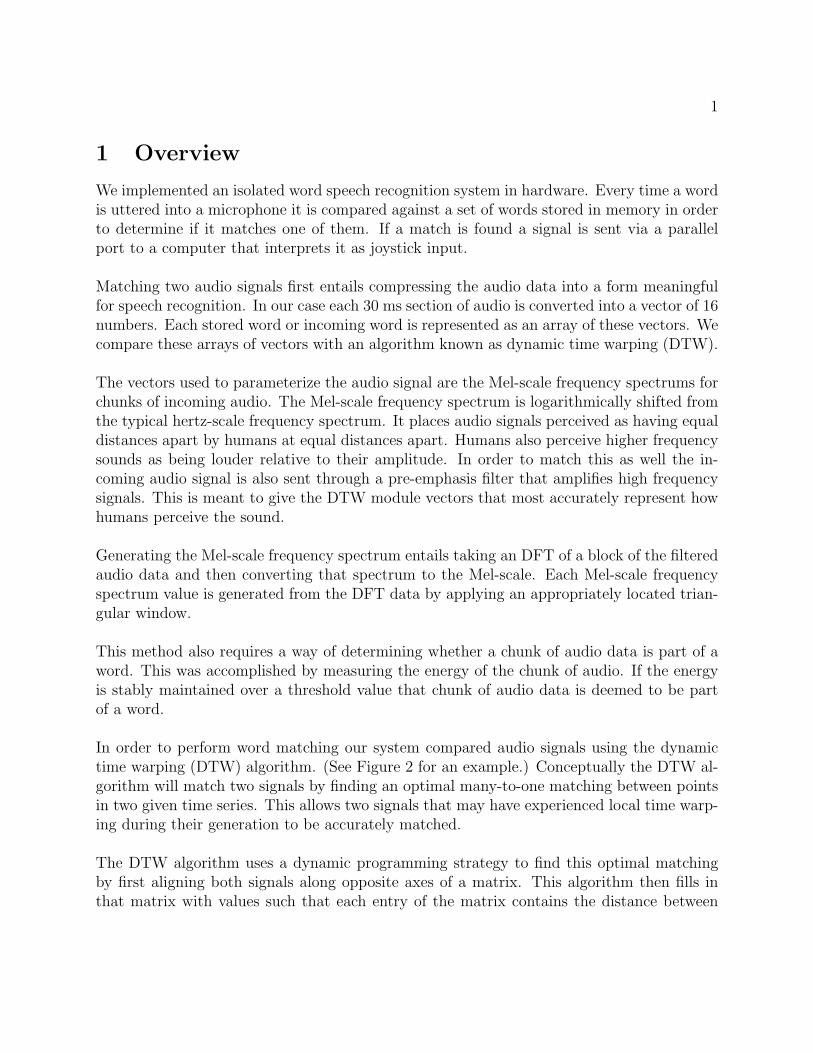
The vectors used to parameterize the audio signal are the Mel-scale frequency spectrums forchunks of incoming audio. The Mel-scale frequency spectrum is logarithmically shifted fromthe typical hertz-scale frequency spectrum. It places audio signals perceived as having equaldistances apart by humans at equal distances apart. Humans also perceive higher frequencysounds as being louder relative to their amplitude. In order to match this as well the in-coming audio signal is also sent through a pre-emphasis filter that amplifies high frequencysignals. This is meant to give the DTW module vectors that most accurately represent howhumans perceive the sound.

Generating the Mel-scale frequency spectrum entails taking an DFT of a block of the filteredaudio data and then converting that spectrum to the Mel-scale. Each Mel-scale frequencyspectrum value is generated from the DFT data by applying an appropriately located trian-gular window.

This method also requires a way of determining whether a chunk of audio data is part of aword. This was accomplished by measuring the energy of the chunk of audio. If the energyis stably maintained over a threshold value that chunk of audio data is deemed to be partof a word.

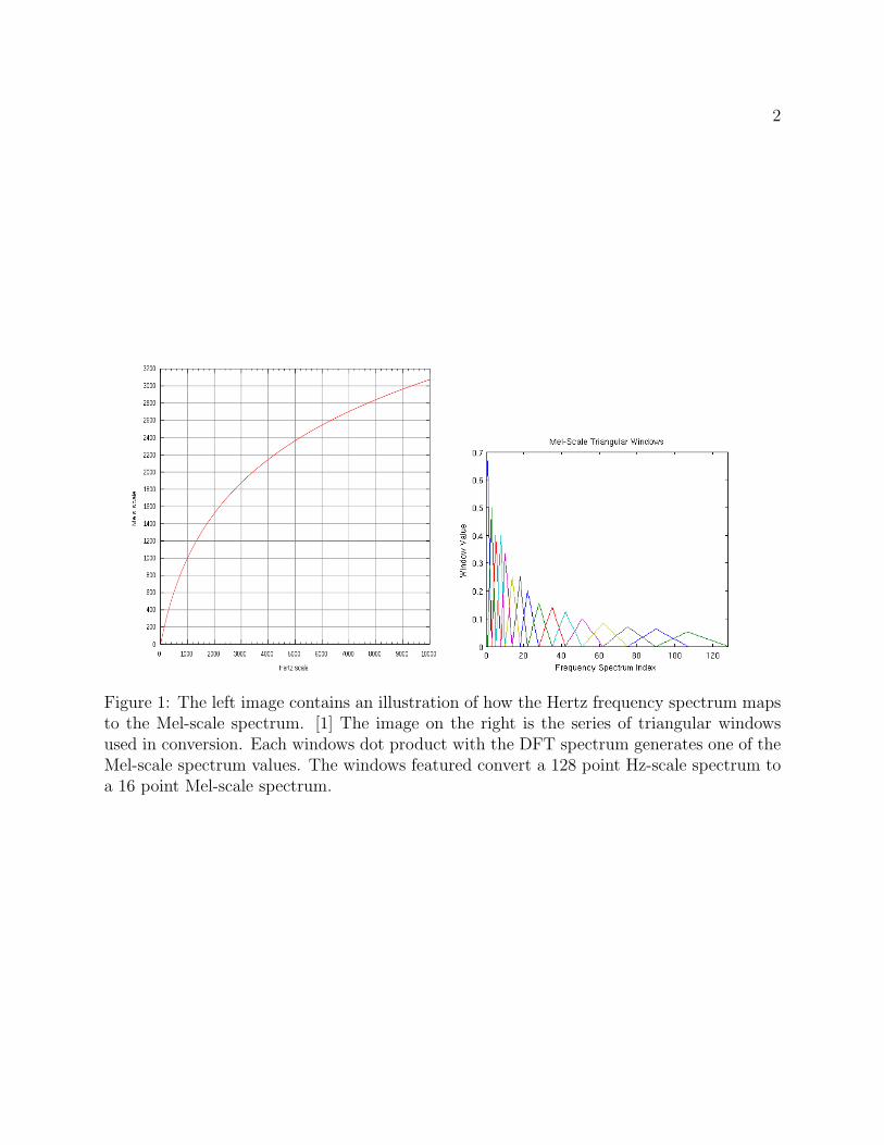
In order to perform word matching our system compared audio signals using the dynamictime warping (DTW) algorithm. (See Figure 2 for an example.) Conceptually the DTW al-gorithm will match two signals by finding an optimal many-to-one matching between pointsin two given time series. This allows two signals that may have experienced local time warp-ing during their generation to be accurately matched.

The DTW algorithm uses a dynamic programming strategy to find this optimal matchingby first aligning both signals along opposite axes of a matrix. This algorithm then fills inthat matrix with values such that each entry of the matrix contains the distance between

2

Figure 1: The left image contains an illustration of how the Hertz frequency spectrum mapsto the Mel-scale spectrum. [1] The image on the right is the series of triangular windowsused in conversion. Each windows dot product with the DFT spectrum generates one of theMel-scale spectrum values. The windows featured convert a 128 point Hz-scale spectrum toa 16 point Mel-scale spectrum.

3

Figure 2: Example of conceptual DTW algorithm execution. [2]

4

it’s row’s associate value and it’s column’s associated value. Finally the algorithm findsthe minimum weight path from the corner of the matrix corresponding to the beginning ofboth series to the opposite corner, which corresponds to the end of both time series. Thisminimum weight path consists of entries in the computation matrix that are each connectedto previous adjacent entries either from below, from the left, or from the intervening diago-nal. The resultant path therefore corresponds directly to the optimal many-to-one mappingbetween discrete points in the two given signals.

To efficiently match a new input word with a set of known words each DTW module storesa trained word in memory and new input words are fed to each DTW module in parallel.Each module executes the DTW algorithm and reports the distance value of the minimumweight path found.

To finally determine if a word match occurred the output of every DTW module is given toa single “judge” module that finds the best reported distance value and determines if thatdistance is within some specified threshold. If this is found to be the case, the correspondingDTW is declared to be the winner for that particular input.

1.0.1 MATLAB Implementation

The preprocessing and DTW algorithm were tested in MATLAB before being implementedin hardware. The website http://www.speech-recognition.de/matlab-files.html pro-vided some of the preprocessing employed. This encompassed taking an FFT and thengenerating the Mel-scale frequency spectrum. We then added pre-emphasis filters, the cal-culation of cepstral coefficients, and the DTW algorithm. The pre-emphasis helped withwords that contained fricatives and the cepstral coefficients proved to be a better param-eterization of audio input. Later during implementation, the MATLAB simulation wouldprovide an excellent framework for testing how our implementation would work under theconstraints provided by trying to implement the algorithm in hardware.

2 Summary of Modules

Our system was divided into two main components: preprocessing and vector generation,and word recognition. Each component was subsequently broken down into interconnectedmodules, which processed the specified input for that component and produced the outputspecified in that components contract. An additional component, system output, was usedto graphically display the function of the system and produce the desired joystick output.

5

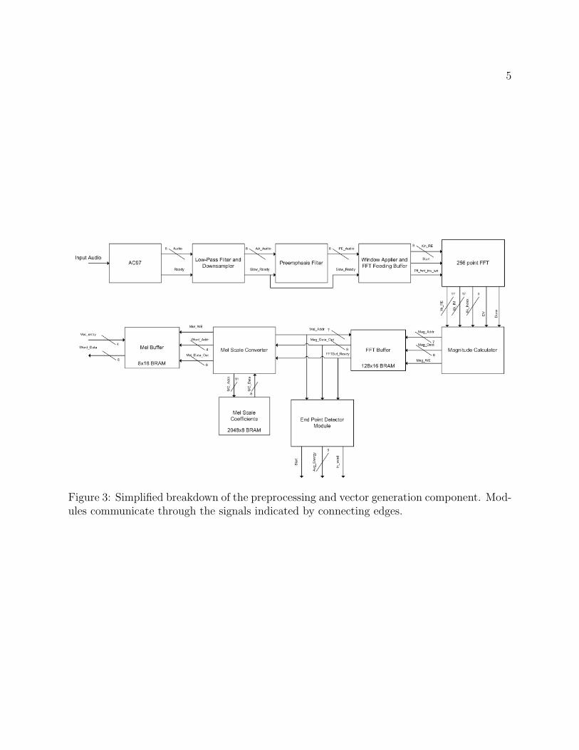
Figure 3: Simplified breakdown of the preprocessing and vector generation component. Mod-ules communicate through the signals indicated by connecting edges.

6

2.1 Audio Preprocessing/Vector Generation

The audio preprocessing takes an 8 bit, 48kHz audio signal and converts into meaningfulvectors for use in the DTW system. This conversion chain encompasses an initial filteringand downsampling stage followed by taking the discrete Fourier transform of a block of theaudio signal. The frequency spectrum generated by the FFT is then converted into a Mel-scale frequency spectrum and the number of values are reduced to 16. These 16 Mel-scalefrequency spectrum values are the parameters used by the DTW modules to match words.The energy of the signal is also calculated and is used to determine when a word is beingsaid into the microphone. Once a block of data reaches the end of the preprocessing chaina signal is sent to the DTW

2.1.1 Discarding Significant Bits

Many of the calculations performed during preprocessing could theoretically generate muchlarger values than they do during typical operation. The discrete Fourier transform, forexample, could generate very large values if the input was consistently a very large value.This is very unlikely to happen, however. In order to keep the size of the circuitry usedduring the calculations down many times during the preprocessing chain significant bitswere discarded. If in the value cannot be represented in the new bit reduced version of thedata, the new data would take the value in the bit reduced form that was closest to what theold would have produced. That typically means the maximum integer possibly representedin the new bit reduced version of the data. In many instances the least significant bits arediscarded. The goal is to have most of the information carried in human speech preservedwhile keeping the size of the circuit down. The number of bits discarded is controlled byparameters programmable at runtime. All of the sections with discarded bits have a directgraphical representation allowing for easy calibration.

2.1.2 Run Time Parameter Control

A set of parameters that affect the preprocessing chain and the word identification arecontrolled via the up and down buttons on the FPGA. The parameter to be modified isselected with a set of switches. These are used to control the discarding of significant bits,the threshold levels for what is considered a word and the timing values associated with wordidentification, and the threshold values for word matches.

2.1.3 Low Pass Filter and Downsampler

The low pass filter is a 31 tap digital finite impulse response (FIR) filter. It is set tofilter frequencies above 3.7 kHz which is above the range of normal human speech. Thecoefficients were generated using matlab and then scaled by 210 and rounded in order to

7

make the coefficients integer values. The incoming 8 bit 48 kHz signal from the AC 97microphone data is sent through the low pass filter and then is downsampled to 8kHz bytaking every 6th value. The data is then passed to the pre-emphasis filter.

2.1.4 Pre-emphasis Filter

The pre-emphasis filter amplifies higher frequencies relative to lower frequencies in order tohave the DFT spectrum better reflect the human response to audio because we perceivehigher frequencies as louder relative to the energy in the signal. This is also a FIR digitalfilter. The coefficients have the form 1 − /α for α ∈ (0, 1). For our use α ≈ 2/5. Thecoefficients were scaled by 29 and rounded. These were then fed to the Window Applier.

2.1.5 Window Applier

The window applier repeatedly applies a Hann window to the incoming data to reduceleakage in the FFT. This multiplies incoming audio data by coefficients representing thewindow stored in a ROM. In order ensure it is synchronized with the buffer feeding theFFT, the window applier is reset whenever the FFT buffer sends data to the FFT.

2.1.6 FFT Feeding Buffer and FFT

The FFT feeding buffer stores incoming samples until it has 256 8 bit samples. At this pointit stops receiving data, sends the appropriate control signals to the FFT and then dumpsall the data in the buffer to the real input in the FFT. The FFT used is a Xilinx Logi-CORE IP Fast Fourier Transform. For the specifications on this see http://www.xilinx.

com/support/documentation/ip_documentation/xfft_ds260.pdf The module used is an8 bit, 256 point FFT with 16 bits for phase information. It uses the radix-2 burst mode andtruncated rounding. For more information on this topic see the documentation at the URLgiven above.

2.1.7 Magnitude Finder

The magnitude of the complex numbers exiting the FFT was found through a pipelinedcalculation that squared the real and imaginary values, added them together and then tookthe square root. The square root was calculated using a large look up table that could acceptnumbers as large as 12 bits. It returned 4 times the square root of the number in order toprovide slightly better data for output. The values exiting the magnitude finder were passedto two block RAMs. One stores data to accessed by a display module. The other stores datato be accessed by the Mel-scale spectrum calculator.

8

2.1.8 Mel-scale Spectrum Calculator

The Mel-scale spectrum calculator is meant to take the 128 unique values coming out ofthe magnitude finder representing the frequency spectrum of the incoming audio data andconvert it into 16 numbers representing the Mel-frequency spectrum. The Mel-frequencyspectrum reflects how humans perceive sound.

If we consider the 128 value data as an incoming vector, then this was accomplished by per-forming the dot product of the incoming vector with 16 vectors that are triangular windowsspaced such that they produce the desired Mel-scale spectrum. The 16 values are stored inthree buffers. One to be used for a graphical display, one to be sent to the DTW modulesand one to be sent to the Cepstral coefficient generator.

2.1.9 Energy Finder and Word Detector

The energy is found using the same hardware as the Mel-scale Spectrum Calculator. Insteadof feeding in a vector representing a triangular window, however, it sends in two versions ofthe 128 point frequency spectrum. Their dot product is the energy. The energy value is thenused to determine if this segment of audio is part of a possible word. If the energy is above acertain threshold value for a set number of incoming energy values then it is deemed a word.If it drops below that energy value for another set number of incoming energy values it is nolonger deemed a word. These delays exist to ensure that multisyllabic words are counted asone word.

Once the Mel-scale values are calculated and whether they are part of a word is determineda signal is sent to the DTW modules signalling that a new block of data is ready.

2.1.10 Cepstral Coefficient Generator

During MATLAB simulations before implementation cepstral coefficients were found to bea better parameterization of the audio data. In our hardware implementation the Mel-scalespectrum values proved to be a better parameterization. This is partly due to instabilitiesin the phase of the cepstral values. Calculating cepstral values involved taking a square rootof the Mel-scale spectrum values and then taking the real part of the output of an IDFT. Avestigial graphical output of them exists.

2.2 Word Recognition

2.2.1 Master

In the original design of our the word recognition component we used a master module tocontrol all of our DTWs and maintain synchronicity in starting their execution. However

9

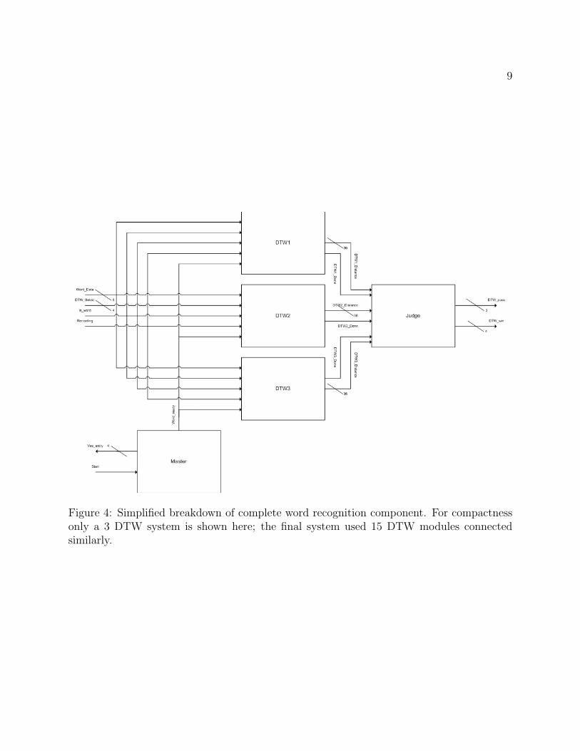
Figure 4: Simplified breakdown of complete word recognition component. For compactnessonly a 3 DTW system is shown here; the final system used 15 DTW modules connectedsimilarly.

10

a redesign of the DTW implementation to stream the computation for matching of a newinput signal removed the need for this master module, as all DTW modules could listen tothe same data bus from the vector generator and manage themselves individually.

There was need for a simple module that acted between the Vector Generator and the jury(the array of 15 DTW modules.) The Vector Generator produced new vectors by filling ina small BRAM and generating a signal when that BRAM had new data available. In orderto satisfy the input specifications of the DTW module an additional module was neededto access the values stored in this BRAM such that it would return its data to the DTWmodules according to their specification. In addition this module needed to generate theappropriate word ready signal for those DTW modules. Fortunately a similar module wasnecessary for unit testing the DTW module, so this module was modified and used as asimple “master” module to deliver new data to all of the DTW modules simultaneously.

2.2.2 DTW

The primary module in the Word Recognition component was the Dynamic Time Warping(DTW) module. This module received input from the Vector Generation component via theMaster and performed one of two functions. In the training mode the DTW module wouldrecord the input it had received, treating that input word as training data. In the testingmode the DTW module will process incoming data as a word sample against which it shouldattempt to match.

Inputs and Parameters Parameter ID: Unique identifier for each DTW module. It isassumed that all DTW ID’s are greater then 0.

Input word data: Bus containing word data, delivered in a packet of 16 8-bit valuessent in succession for each vector.

Input word ready: 1 clock cycle pulse that indicates the availability of new data (thefirst entry in a vector) on the word data bus.

Input in word: Level signal to indicate a set of contiguous vectors that compose a singleword.

Input dtw select: Bus indicating which DTW is currently being trained, or 0 whenDTWs should attempt to match new input.

Input recording: Level signal indicating when the selected DTW should attempt tostore an incoming word as a training sample.

11

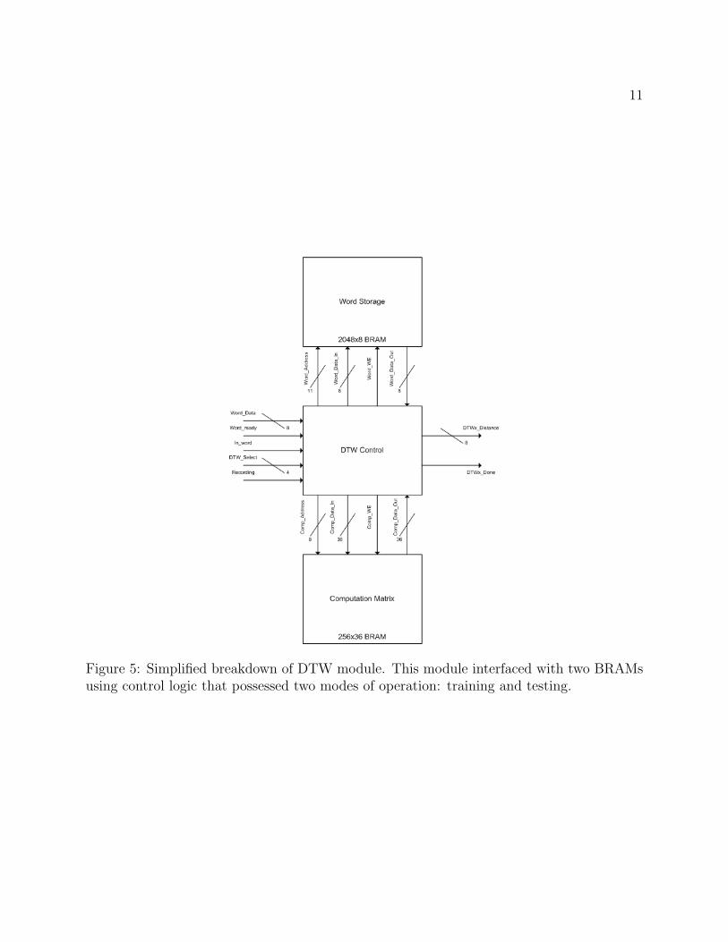
Figure 5: Simplified breakdown of DTW module. This module interfaced with two BRAMsusing control logic that possessed two modes of operation: training and testing.

12

Components and Operation The DTW module has two modes of operation: trainingand testing.

Each DTW module contained a BRAM for storing a new training word. This BRAM wascapable of storing 128 16-entry vectors of 8-bit words. The Vector Generation componentproduced one such vector for each time slice of input data in a word, and because eachvector represented approximately 32 ms of input data a full BRAM would corresponded toa maximum word length of 4 seconds. This corresponds to a very long word; most wordsexamined during testing consisted of at most 24 samples. Therefore, for simplicity, we de-cided not to concern ourselves with potentially overflowing this training word storage BRAM.

To control this training word BRAM, each DTW possessed a small amount of recording con-trol logic. This logic examined to determine if the DTW was currently selected for training,(dtw select equaled the DTW’s ID) the user was recording, and the in word signal was high.If all of these were true, then new word data received, packets of which were indicated viathe “word ready” signal, were stored in the training word BRAM. If the word ended and anew word began while the “recording” signal was engaged, the latter word would overwritethe first word, allowing the user to retrain a single DTW without imposing a full reset ofthe system.

When the DTWs were not engaged in training mode (dtw select was 0) new word datawould be processed in testing mode. In this mode the DTW module evaluated one row ofthe computation matrix at a time. When the DTW module received a complete vector itwould treat that vector as the next value in the testing input, and compute the distancebetween that vector and every stored vector in that DTW’s trained word. Meanwhile theDTW module would use the previously computed row of values to determine the distancesof the minimum weight paths to each cell in the new row, and subsequently combine thosepath values with the distances associated with entry to compute complete path length valuesfor the new row.

At the end of this computation the weight of the minimum weight path to the final cellexamined corresponded to the minimum weight path in the complete matrix for the wordreceived thus far. Therefore if the in word signal went low after this vector, indicating theend of the word, the DTW module may simply return this last computed net distance valueand indicate that it had completed.

This strategy for computation had a number of advantages. Because the DTW computationfor each row depended only on the previously computed row in the computation matrix, only

13

two rows of this matrix had to be stored at any time. Because each new vector was receivedat least 32 ms apart, an entire row of the DTW computation matrix could be computedbefore the reception for the next vector. This removed the necessity of our algorithm tostore an entire word for matching purposes, and allowed the DTW modules to return almostimmediately upon receiving a signal of the end of the word (in word going low.) The endresult of this strategy is therefore increased efficiency and a smaller memory requirementfor each DTW. These optimizations to the DTW module were important, since we wereplanning on using a large number of DTW modules (15) and desired low latency from oursystem.

2.2.3 Judge

The judge module took distance values and completion signals from all DTW modules anddetermined which of those DTWs successfully matched the last input word. The judge uti-lized two metrics to determine if a match was found. First it examined all distances returnedby the DTW modules and examined if they were below some pre-specified threshold value.Second, if examined the distance from all DTW modules to determine which was gave thesmallest distance.

The judge module produced two output signals. First it produced a bus of values indicatingwhich DTWs had produced a distance value that was within the specified threshold. Secondit produced the ID of the “winning” DTW, where a DTW could only win if it produced thesmallest measured distance of any other module and that value was less then the specifiedthreshold. This output was subsequently processed by the DTW display modules and thejoystick module, or “executioner,” to produce the desired output to the user.

2.3 System Output

Our system had two forms of output. First, to visually observe its processing and fordebugging purposes, we incorporated a number sprite modules to print pertinent data to thedisplay. Second, we incorporated a joystick interface module to translate word recognitioninto joystick button presses and to interface with a computer as a joystick.

2.3.1 Bar Graph Display

The hertz scale frequency spectrum values, the Mel-scale frequency spectrum values, and theCepstral coefficients are all displayed on a VGA display. They are displayed as bar graphsthat update everytime a packet of audio data is sent through the processing chain. They areimplemented as sprites that are sent a pixels position and return the color one clock cyclelater. The heights of the bars are stored in a BRAM that updates during the vsync pulse.

14

2.3.2 DTW Display

For debugging and visualization purposes, each DTW was connected to a display modulethat would display pertinent data concerning the DTW. Each DTW display module dis-played the DTW’s ID and associated distance value. The DTW displays were clusteredbased on the intended usage pattern of our system, where three DTW modules would betrained for each word.

This text display would assume a different color depending on the status of that DTW’soutput, as determined by the associated DTW module and the judge. If the DTW was pro-cessing (dtw done was low) the text for that DTW would be displayed in white. Otherwise, ifthe judge had determined that DTW’s distance value had failed to beat the stored thresholdvalue, this text would be displayed in red. If the distance value returned by the DTW waswithin the threshold limit, the display for that module would be colored cyan. Finally, if thejudge determined that the particular value produced by a DTW was within the thresholdlimit and was the best value of those returned by any DTW module, that DTW’s displaywould display green text, indicating the winning module.

2.4 Joystick Output

Joystick output is generated following the protocol used by Playstation 1 controllers. This isa basic serially protocol done over four data lines. All of the incoming data was sent througha debouncer before interacting with the controller circuitry. With the modification of a fewtiming parameters the communication protocol will also work with a PS2. To interface thisto a computer we relied on a freeware program named PSX Pad. For more information onthe protocol see http://users.ece.gatech.edu/~hamblen/489X/f04proj/USB_PSX/psx_

protocol.html.

3 Testing

A series of tests were performed to debug and examine the effectiveness of our system. Firsteach component was tested through a series of unit tests and component-wide integrationtests. Once both components were found to be working properly they were combined andfull system integration tests were performed. Finally we performed controlled experimentsto examine the effectiveness of our algorithm and gameplay tests to examine its performancein an example application.

3.1 Unit Testing

We performed individual unit testing on the preprocessing and word recognition components.

15

3.1.1 Preprocessing

The coefficients for the two filters were first tested on simulated audio data in MATLAB.The actual Verilog implementation was then tested with simulated audio data in Modelsim.The window applier was tested by generating canned input and viewing the output on a logicanalyzer. The FFT feeding buffer was also sent predetermined data and then the outputwas observed to make sure it met all the timing specs of the FFT and presented the properdata. The Xilinx FFT was given a few delta pulses with known responses in order to testcorrectness. The magnitude finder was tested with a set of inputs. The hardware used toimplement the Mel-spectrum calculator was tested with Modelsim.

3.1.2 Word Recognition

The most complex module in the Word Recognition component was the DTW module it-self, so it in particular was subjected to a substantial amount of careful testing. The DTWmodule was first simulated using ModelSim in order to ensure the correct synchronizationof internal signals for accessing the storage and computation matrix BRAMs as well as forperforming the computation pipelines to execute the DTW algorithm.

Once these signals were verified the DTW module was tested on the FPGA itself. A simplemodule that would eventually become the Master was created to access preloaded BRAMsof values and feed their contents to the DTW modules according to their specification.These preloaded BRAMs were loaded with specific values to examine different aspects of theDTW’s execution. For example, two identical BRAMs were used for training and testing ofthe DTW module to ensure that the distance produced was 0. More complex sets of trainingand testing BRAMs whose distance value according to DTW was known were also tested toensure the correctness of the computation.

Finally the Judge and DTW Display modules were connected to a single DTW module toverify the correctness of both of these modules and the word recognition component as awhole. We first tested a complete word recognition component that incorporated a singleDTW module. Once the proper functionality of this setup was observed we connected moreDTW modules to the system and verified their parallel functionality.

3.1.3 Experimentation

We performed a few tests to gain a sense of the error rates of our system. Two sets of testswere performed; one where each DTW trained stored a unique word, and one where sets ofthree DTWs were trained per word. This initial set of tests examined the performance of thealgorithm itself, while the latter tests examined more closely the performance of the system

16

as we planned to use it in gaming applications.

To complement our initial Matlab tests between the words “taco” and “fish” we examinedour system’s recognition of these two words. Each word was uttered 10 times, and thenumber of matches for each word was recorded. The vertical chart of the following graphdescribes the two words trained into the system, while the horizontal axis describes the wordbeing used to test.

Trained Word fish taco

fish 10 0taco 0 10

As expected based on our initial experimentation with Matlab, our algorithm was able toeffectively distinguish the words “fish” and “taco,” scoring perfect results.

We then subjected our algorithm to two more challenging tests. First it’s ability to dis-tinguish “pot‘ay’to” from “pot‘ah’to,” and results given below were found. Again, for theresults below, each word was uttered 10 times, and the number of matches for each trainedis recorded; missing entries indicate instances where the utterance failed to match any word.

Trained Word pot‘ay’to pot‘ah’to

pot‘ay’to 9 0pot‘ah’to 1 4

In these tests we found significantly more errors on account of the significantly more similarwords. One false positive was discovered, and the system had difficulty matching pot‘ah’tomany times. The higher word similarity is the most likely cause of the mismatch discovered.The failed matches are probably due to a sub-par training recording or the pre-emphasisfilter, which amplified the higher frequencies in an attempt to make our system better ableto handle fricatives.

The final algorithmic test we attempted, and arguably the most difficult, attempted to dis-tinguish the words “alpha,” “bravo,” “charlie,” and “delta” from each other. In this caseeach word was uttered 5 times, yielding the results depicted below.

Trained Word alpha bravo charlie delta

alpha 5 1 0 3bravo 0 4 0 0charlie 0 0 2 0delta 0 0 0 2

This test demonstrated some significant problem areas in our algorithm. First, our algorithmhad difficulty detecting the utterance of a fricative, due to the high-frequency low-magnitude

17

nature of fricatives. This accounts for the lack of successful matches with the word “charlie,”since that test point starts with a fricative-like sound. This test also compared two wordsthat sounded very similar: “alpha” and “delta.” Unsurprisingly our algorithm had diffi-culty distinguishing such similar words from each other, matching each word approximatelyequally when the uttered word was “delta.” This may be due to the soft or quiet nature ofthe initial consonant, which may not have been detected by our system in many cases.

To combat high error rates when used in practical applications we decided to operateour system with 3 DTWs trained on 3 instances of each word. We conducted similar error-rate tests with this modified configuration, using words of more pertinent interest to thesystem’s intended use. In both of the tests described below, each word was uttered 10 timesin testing, and a word match was counted if any of the DTWs associated with some wordsuccessfully matched the input. First we examined the error rates when given the words“up” and “down.”

Trained Word up down

up 10 0down 0 10

Next we examined the error rates when given the words “left” and “right.”

Trained Word left right

left 9 1right 1 9

With this modification to the application of our algorithm we were able to achieve substan-tially better error rates on words we expected our system to handle. This result demonstratedpromise for our system to effectively recognize words in a gaming setting.

3.1.4 Gameplay Testing

Thanks to a once flourishing emulation community on the internet there is software thattranslates joystick input into mouse or keyboard input. This means that the joystick inputgenerated by the hardware can be used for a large number of tasks on the computer. Wetested the input with two different uses. The first use was using the joystick input on thecomputer to control NES games on an emulator. Because of the slight delay inherent in thevoice processing complete control of the games proved to be problematic. Using the inputto supliment the controls already was a much better idea. Mapping the word “away” to thebutton that launches bombs in 1942 for example. That way when you say “bombs away” itactually happens.

We also used the input to drive a very simple python script that, when it received certain

18

joystick input, played an audio file with “do doo do do doo.” Training the speech recognitionsystem on “Mahna Mahna” allowed us to reenact that bit. If you have no idea what I amtalking about see http://muppet.wikia.com/wiki/Mahna_Mahna_(song).

4 Conclusion

We implemented an isolated word speech recognition system in hardware. This systemprocesses raw audio data using Mel scale values and matches words using the dynamic timewarping algorithm. We have successfully demonstrated this systems capability to distinguishmany words from each other, through use of our algorithm and through the use of multipleDTW modules trained on the same word. Finally we implemented a joystick interface to ourspeech recognition system that allows it to interface with an existing computer and executejoystick button press commands through word recognition.

Our system works well at distinguishing dissimilar words from each other. However there area number of points in which recognition does not work as well. Words that begin or end withfricatives often have difficulties on account of the high-frequency nature of fricative soundsfailing to generate sufficient energy for the system to detect. In a future implementationwe may attempt to combat this effect with a pre-emphasis filter that amplified higher fre-quencies, although initial testing with such a filter tended to increase these higher frequencyvalues too much, hurting the system’s ability to match words.

Very short words tend to match much more frequently, since the dynamic time warping al-gorithm will tend to find a good matching with such short inputs. We attempted to combatthis effect by adding a small punishment value for matching words of dramatically differentlengths, but properly calibrating this punishment value proved tricky on initial implementa-tion.

In general we found that our algorithm was effective at matching words and identifying thecorrect word from the best distance value. However reasonable threshold values were difficultto determine, and different length words often needed different threshold values. Dynamicthreshold values based on word lengths may be useful to implement to improve our system’seffectiveness in the future.

As mentioned previously Matlab tests indicated that cepstral coefficients would be moreeffective for speech recognition applications then mel scale values. We attempted to imple-ment this feature, but due to phase instability in the inverse FFT output we were unable tomake effective matches on these values. Future work should investigate this instability andattempt to counteract it to provide more effective matches.

19

Overall our system worked reasonably well at isolated word speech recognition. We weresuccessful in applying a joystick interface to our speech recognition system that allowed usto play games and perform a variety of tasks on a computer using a voice interface. Thereare a number of areas in which our speech recognition system could be improved, but oursystem overall achieved reasonable success.

20

References

[1] http://en.wikipedia.org/wiki/Mel_scale . Images of Mel Scale borrowed fromwikipedia. November 2008.

[2] Keogh, Eamonn and Michael Pazzani. Derivative Dynamic Time Warping. Example im-age of DTW execution borrowed from this paper. November 2008.