speculative bubbles and financial crisis · with incomplete –nancial markets and borrowing...
TRANSCRIPT
Research Division Federal Reserve Bank of St. Louis Working Paper Series
Speculative Bubbles and Financial Crisis
Pengfei Wang
and Yi Wen
Working Paper 2009-029B
http://research.stlouisfed.org/wp/2009/2009-029.pdf
June 2009 Revised July 2009
FEDERAL RESERVE BANK OF ST. LOUIS Research Division
P.O. Box 442 St. Louis, MO 63166
______________________________________________________________________________________
The views expressed are those of the individual authors and do not necessarily reflect official positions of the Federal Reserve Bank of St. Louis, the Federal Reserve System, or the Board of Governors.
Federal Reserve Bank of St. Louis Working Papers are preliminary materials circulated to stimulate discussion and critical comment. References in publications to Federal Reserve Bank of St. Louis Working Papers (other than an acknowledgment that the writer has had access to unpublished material) should be cleared with the author or authors.

Speculative Bubbles and Financial Crisis�
Pengfei WangHong Kong University of Science & Technology
Yi WenFederal Reserve Bank of St. Louis
& Tsinghua University (Beijing)
July 23, 2009
Abstract
Why are asset prices so much more volatile and so often detached from their fundamental values? Why
does the bursting of �nancial bubbles depress the real economy? This paper addresses these questions by
constructing an in�nite-horizon heterogeneous agent general equilibrium model with speculative bubbles.
We characterize conditions under which storable goods, regardless of their intrinsic values, can carry
bubbles and agents are willing to invest in such bubbles despite their positive probability of bursting.
We show that perceived changes in the bubbles�probability to burst can generate boom-bust cycles and
produce asset price movements that are many times more volatile than the economy�s fundamentals, as
in the data.
Keywords: Asset Price Volatility, Boom-Bust Cycles, Financial Crisis, Speculative Bubbles, Sunspots,
Tulip Mania.
JEL Codes: E21, E22, E32, E44, E63.
�We thank Judy Ahlers and Luke Shimek for research assistance. The usual disclaimer applies. Correspondence: Yi Wen,Research Department, Federal Reserve Bank of St. Louis, St. Louis, MO, 63144. Phone: 314-444-8559. Fax: 314-444-8731.Email: [email protected].
1
1 Introduction
The current �nancial crisis caused by the burst of the U.S. housing bubble is not new. History has too often
witnessed the rise and collapse of nationwide asset bubbles. Each time, an entire economy cheered for a
bubble�s birth and then mourned its death. The �rst recorded nationwide bubble is the "Tulip mania"� a
period in Dutch history during which contract prices for tulip bulbs reached extraordinarily high levels and
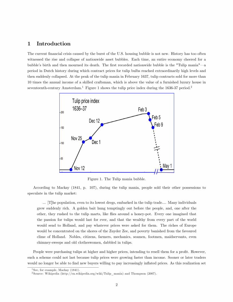
then suddenly collapsed. At the peak of the tulip mania in February 1637, tulip contracts sold for more than
10 times the annual income of a skilled craftsman, which is above the value of a furnished luxury house in
seventeenth-century Amsterdam.1 Figure 1 shows the tulip price index during the 1636-37 period.2
Figure 1. The Tulip mania bubble.
According to Mackay (1841, p. 107), during the tulip mania, people sold their other possessions to
speculate in the tulip market:
... [T]he population, even to its lowest dregs, embarked in the tulip trade.... Many individualsgrew suddenly rich. A golden bait hung temptingly out before the people, and, one after the
other, they rushed to the tulip marts, like �ies around a honey-pot. Every one imagined that
the passion for tulips would last for ever, and that the wealthy from every part of the world
would send to Holland, and pay whatever prices were asked for them. The riches of Europe
would be concentrated on the shores of the Zuyder Zee, and poverty banished from the favoured
clime of Holland. Nobles, citizens, farmers, mechanics, seamen, footmen, maidservants, even
chimney-sweeps and old clotheswomen, dabbled in tulips.
People were purchasing tulips at higher and higher prices, intending to resell them for a pro�t. However,
such a scheme could not last because tulip prices were growing faster than income. Sooner or later traders
would no longer be able to �nd new buyers willing to pay increasingly in�ated prices. As this realization set
1See, for example, Mackay (1841).2Source: Wikipedia (http://en.wikipedia.org/wiki/Tulip_mania) and Thompson (2007).
2

in, the demand for tulips collapsed and prices plummeted. The Dutch economy went into a deep recession
in 1637.
Although historians and economists continue to debate whether the tulip mania was indeed a bubble
caused by what Mackay termed "Extraordinary Popular Delusions and the Madness of Crowds" (see, e.g.,
Dash, 1999; Garber, 1989, 1990; and Thompson, 2007), this paper shows that genuine bubbles with prices
far exceeding the bubbles�fundamental values and with movements similar to Figure 1 can be constructed
in an in�nite-horizon dynamic stochastic general equilibrium (DSGE) model. In the model, in�nitely lived
agents are willing to invest in bubbles even though they may burst at any moment. The reason is that
with incomplete �nancial markets and borrowing constraints, bubbles provide liquidity and help diversify
idiosyncratic risks by serving as stores of value. We show that the burst of such bubbles can generate
recessions, and the perceived changes in the probability of the bubbles�burst can cause asset price movements
many times more volatile than aggregate output.
People invest in bubbles for many reasons. The idea that in�nitely lived rational agents are willing to
hold bubbles with no intrinsic values to self-insure against idiosyncratic income risks can be traced back
at least to Bewley (1980).3 This idea is more clearly articulated recently in general equilibrium models by
Kiyotaki and Moore (2008) and Kocherlakota (2009), where heterogeneous �rms use intrinsically worthless
assets to improve resource allocation and investment e¢ ciency when �nancial markets are incomplete.4
This paper extends this literature to study asset price volatility and bubbles that may grow on assets with
intrinsic values. This extension is not trivial because sunspot equilibrium may disappear in the Kiyotaki-
Moore-Kocherlakota model once the object supporting the bubble (e.g., land) is allowed to have fundamental
values. More importantly, casual observation suggests that more often the bubbles are likely to exist in goods
with fundamental values, such as antiques, bottles of wines, paintings, �ower bulbs, rare stamps, houses,
land, and so on.
We use a DSGE model to characterize conditions for the existence of rational bubbles that grow on
goods with fundamental values. We show that any inelastically supplied storable goods,5 regardless of
their intrinsic values, can support bubbles with the following features: (i) the market price of the goods
exceeds their fundamental values and (ii) the market values can collapse to fundamental values with positive
probability (namely, the fundamental value is itself a possible equilibrium).6
The basic structure of our model closely resembles that of Kiyotaki and Moore (2008) and Kocherlakota
(2009) wherein �rms, instead of households, invest in bubbles; however, the analysis easily can be extended
to households. The main di¤erences between our model and the literature include the following:
1. In addition to characterizing general equilibrium conditions for bubbles to develop on objects with
fundamental values, in our model the probability of capital investment is endogenously determined by
�rms rather than exogenously �xed. That is, �rms optimally choose whether to invest in �xed capital
3 It can be traced further back to Samuelson�s (1958) overlapping generations model of money. For a recent extension ofBewley�s model to a DSGE model with multiple assets; see Wen (2009).
4The related literature also includes Angeletos (2007), Araujo, Pascoa, and Torres-Martinez (2005), Caballero and Krish-namurthy (2006), Farhi and Tirole (2008), Hellwig and Lorenzoni (2009), Kocherlakota (1992), Santos and Woodford (1997),Scheinkman and Weiss (1986), Tirole (1985), and Woodford (1986), among others. These literature reports focus on asset pricebubbles and �nancial market frictions and di¤er from the indeterminacy literature of Benhabib and Farmer (1994) and Wangand Wen (2007, 2008). For the earlier literature on sunspots, see Cass and Shell (1983) and Azariadis (1981).
5Goods can be producible yet at the same time inelastically supplied. For example, antiques and bottles of wine are producedgoods, but their dates of production make them unique and nonsubstitutable by newly produced ones.
6 If the fundamental value is not an equilibrium, then bubbles will never burst and thus it may be argued that bubblesdo not exist (because it is di¢ cult to know empirically whether there is a bubble if it never bursts). Also, the existence ofmultiple fundamental equilibria does not imply bubbles because the asset values never exceed fundamentals in a fundamentalequilibrium.
3
each period. Hence, in equilibrium the number of �rms that are investing can respond to aggregate
shocks and monetary policy. This extensive margin is missing from the literature.
2. We introduce multiple assets in the model. Our multiple asset approach allows us to construct sto-
chastic sunspot equilibrium and conduct impulse response analyses and time-series simulations.
3. We focus on asset price volatility and calibrate our model to match the second moments of the U.S.
data.
4. We provide an analytically tractable method to solve the dynamic paths of our model (without re-
sorting to numerical computational techniques as in Krusell and Smith, 1998) despite a continuum of
heterogeneous agents with irreversible investment and borrowing constraints.7
The rest of the paper is organized as follows. Section 2 presents a basic model and characterizes conditions
under which bubbles can grow on goods with intrinsic values. Section 3 introduces sunspot shocks to a version
of the basic model (by allowing the perceived probability of bubbles to burst to be stochastic) and calibrates
the model to match the U.S. business cycles and asset price volatility. Section 4 concludes the paper.
2 The Basic Model
2.1 Firms
There is a continuum of competitive �rms indexed by i 2 [0; 1]. Each �rm maximizes discounted dividends,
E0P1
t=0 �t�tdt(i); where d denotes dividend, � the representative household�s marginal utility that �rms
take as given, and � 2 (0; 1) the time-discounting factor. The production technology of �rm i is denoted by
y(i) = Ak(i)�n(i)1��; � 2 (0; 1); (1)
where A is an index of aggregate total factor productivity (TFP), k(i) capital stock, and n(i) employment.
The capital stock is accumulated according to the law of motion:
kt+1(i) = (1� �)kt(i) +it(i)
"t(i); (2)
where investment is irreversible (i(i) � 0) and is subject to an idiosyncratic rate of return (cost) shock, "t(i);with support, [";�"] 2 R+; and the cumulative distribution function, F (").Assume that in the beginning of time (t = 0) there exists one unit of divisible good endowed from nature
and equally distributed among the �rms. The good can be paid to households (�rm owners) as dividends
and yield marginal utility, f . Hence, f is the fundamental value of the good.8 (We call the good "tulips"
throughout the paper.) Also assume that households do not have the technology to store tulips but �rms
do, and there exists a �xed storage cost, � � 0; per unit per period. Obviously, �rms will never want to selltulips if their market price, (q), is less than f . The question is: Do �rms have incentives to hold and invest
in tulips when q > f? In other words, can q > f be supported as a competitive (bubble) equilibrium in the
economy other than the fundamental equilibrium, q� = f? Intuitively, because tulips are storable for �rms,
7Our method follows that of Wang and Wen (2009). As far as we know, the existing literature� except Wang and Wen(2009)� has not shown how to solve discrete-time models with irreversible investment and borrowing constraints analytically.
8For simplicity, assume that the good cannot be used as a factor of production.
4

they thus allow a �rm to self-insure against idiosyncratic shocks by serving as a store of value (i.e., liquidity).
For example, if the cost shock " is large (or the rate of return to capital investment is low), �rms may opt
to invest in tulips to have liquidity available in the future when the next-period costs of capital investment
may be low. On the other hand, if the rate of return to capital investment is high (" is small), �rms may opt
to liquidate (sell) tulips in hand and make more income available by purchasing �xed capital and expanding
production capacity. Such behavior is rational despite the fact that tulip bubbles have a positive probability
to burst.
To characterize the conditions for the existence of a bubble equilibrium, consider a �rm�s maximization
problem, which is to decide whether and how much to invest in tulips to maximize the present value of
expected future dividends. The �rm�s resource constraint is
dt(i) + it(i) + (qt + �)ht+1(i) + wtnt(i) � Atkt(i)�nt(i)1�� + qtht(i); (3)
where w is the real wage, ht+1 the quantity (or shares) of tulips purchased in the beginning of period t as a
store of value, and �ht+1 the total �xed storage costs paid for storing tulips within period t. In addition, we
impose the following constraints: dt(i) � 0 and ht+1(i) � 0. That is, �rms can neither pay negative dividendsnor hold negative amounts of tulips. These assumptions imply that �rms are �nancially constrained and
the asset markets are incomplete. Such constraints plus investment irreversibility give rise to speculative
(precautionary) motives for investing in tulip bubbles.
The following steps simplify our analysis. Using the �rm�s optimal labor demand schedule,
(1� �)Ak(i)�n(i)�� = w; (4)
we can express labor demand as a linear function of the capital stock, k(i),
n(i) =
�(1� �)A
w
� 1�
k(i): (5)
Accordingly, output y(i) is also a linear function of k(i),
y(i) = A
�(1� �)A
w
� 1���
k(i). (6)
These linear relations imply that aggregate output and employment may depend only on the aggregate
capital stock. Thus, we do not need to track the distribution of k(i) to study aggregate dynamics. De�ning
R � �Ah(1��)A
w
i 1���
, the �rm�s net revenue is given by
y(i)� wn(i) = Rk(i); (7)
which is also linear in the capital stock.
Using the de�nition of R, the �rm�s problem is to solve
maxE0
1Xt=0
�t�t [Rtkt(i)� it(i) + qtht(i)� (qt + �)ht+1(i)] ; (8)
5

subject to the following constraints:
dt(i) � 0 (9)
ht+1(i) � 0 (10)
it(i) � 0 (11)
kt+1(i) = (1� �) kt(i) +it(i)
"t(i): (12)
Let f�(i); �t(i); �(i); �(i)g denote the Lagrangian multipliers of constraints (9) through (12), respectively;the �rst-order conditions for fit(i); kt+1(i); ht+1(i)g are given, respectively, by
1 + �t(i) =�t(i)
"t(i)+ �t(i) (13)
�t(i) = �Et�t+1�t
�[1 + �t+1(i)]Rt+1 + (1� �)�t+1(i)
(14)
[1 + �t(i)] (qt + �) = �Et�t+1�t
�qt+1
�1 + �t+1(i)
�+ �t(i); (15)
plus the complementary slackness conditions,
�t(i)it(i) = 0 (16)
�t(i)ht+1(i) = 0 (17)
[1 + �t(i)] [Rtkt(i)� it(i) + qtht(i)� (qt + �)ht+1(i)] = 0: (18)
Notice that equation (14) implies that the value of �t(i) is the same across �rms because "(i) is i.i.d. and is
orthogonal to aggregate shocks.
2.2 Decision Rules
There are two possible outcomes for the circulation of tulips and their liquidation value in the economy.
First, tulips may not be traded among �rms and their liquidation value is simply q = f . Second, tulips
may be traded among �rms and their market price is q � f .9 In the �rst possible outcome, each �rm does
not expect other �rms to invest in tulips and therefore has no incentives to deviate by holding tulips as a
store of value. This may happen, for example, if the liquidation value, f , is low relative to storage costs so
that tulips are not an e¢ cient store of value. In the second possible outcome, each �rm expects a positive
measure of other �rms willing to hold tulips each period and the liquidation value, q; is su¢ ciently high;
thus, it is willing to invest in tulips as well. Which outcome prevails in general equilibrium depends on the
parameter space, as the following analysis shows.
The decision rules at the �rm level are characterized by a cuto¤ strategy. Consider two possibilities:
Case A: "t(i) � "�t . In this case, the cost of capital investment is low. Suppose it(i) > 0; accordinglywe have �t(i) = 0. Equations (13) and (14) imply
"t(i) [1 + �t(i)] = �Et�t+1�t
�[1 + �t+1(i)]Rt+1 + (1� �)�t+1(i)
: (19)
9Notice that in any case, qt < f can never be an equilibrium outcome, because in this case the demand for tulips will riseand consequently qt will increase.
6

Given that �t(i) � 0, we must have "t(i) � �Et�t+1�t
�[1 + �t+1(i)]Rt+1 + (1� �)�t+1(i)
, which de�nes the
cuto¤ value, "�t ;
"�t � �Et�t+1�t
�[1 + �t+1(i)]Rt+1 + (1� �)�t+1(i)
: (20)
Equation (13) then becomes
1 + �t(i) ="�t"t(i)
: (21)
Hence, whenever "t(i) < "�t , we must have �t(i) ="�t"t(i)
� 1 > 0 and dt(i) = 0. Equation (15) becomes
"�t"t(i)
(qt + �) = �Et�t+1�t
�qt+1
�1 + �t+1(i)
�+ �t(i): (22)
De�ning ��t as the cuto¤ value of �t(i) for �rms with "t(i) = "�t , equation (22) implies
qt + � = �Et�t+1�t
�qt+1
�1 + �t+1(i)
�+ ��t : (23)
Given that ��t � 0, the fact that �t(i) > ��t under Case A yields
�t(i) > 0: (24)
That is, for any "t(i) < "�t , we must have
ht+1(i) = 0 (25)
and
it(i) = Rtkt(i) + qtht(i): (26)
This suggests that �rms opt to liquidate all �nancial assets to maximize investment in �xed capital when
the cost of �xed investment is low.
Case B: "t(i) > "�t . In this case, the cost of investing in �xed capital is high. Suppose dt(i) > 0 and
�t(i) = 0. Then equations (13) and (14) and the de�nition of the cuto¤ "� imply �t(i) = 1 � "�t"t(i)
> 0.
Hence, we have it(i) = 0. In such a case, �rms opt not to invest in �xed capital and instead pay shareholders
a positive dividend. Given that �t(i) = 0, equation (15) implies �t(i) = ��t � 0. That is, the Lagrangian
multiplier �(i) is the same across �rms under Case B because ��t is independent of i. However, depending
on the liquidation value of tulips in the next period, there are two possible choices (outcomes) for tulip
investment under Case B: (B1)R 10ht+1(i)di > 0 and (B2)
R 10ht+1(i)di = 0. The �rst outcome (B1) implies
a positive aggregate demand for tulips (i.e., tulips are held as a store of value in the economy) because �rms
expect other �rms to accept tulips in the future and the liquidation value is high enough to cover storage
costs, so we must have ��t = 0. The second outcome (B2) implies that tulips are not traded and all existing
tulips are consumed (i.e., paid to households as dividends); hence, we must have ��t � 0 and ht+1(i) = 0 forall i. Under outcome (B2), we must also have qt = f .
Thus, whether a positive demand exists for tulips under Case B depends on �rms�expectation of the
liquidation value of tulips in the future (i.e., on whether tulips are traded in the next period). Denoting
t+1 �Z 1
0
ht+1(i)di (27)
as the aggregate demand of tulips in period t, the two possible outcomes under Case B imply the equilibrium
7

complementary slackness condition,
t+1��t = 0: (28)
Combining Cases A and B, the decision rule for capital investment is given by
it(i) =
8><>:Rtkt(i) + qtht(i) if "t(i) � "�t
0 if "t(i) > "�t
: (29)
The rate of returns to tulips depends on the expected marginal value of liquidity (cash �ow), which is greater
than 1 because of the option of waiting. This option value is denoted by
Q("�t ) � E [1 + �(i)] =Zmax
�1;"�
"(i)
�dF (") > 1: (30)
When the cost of capital investment is low (Case A), one tulip yields "�
"(i) > 1 units of new capital through
investment by liquidating the tulip asset. When the cost is high (Case B), �rms can opt to hold on to theliquid asset and the rate of return is simply 1.
Using equations (22) and (23), the value of the Lagrangian multiplier for the nonnegativity constraint
(10) is determined by
�t(i) =
8>><>>:�"�
"(i) � 1�(qt + �) if "(i) � "�
��t if "(i) > "�: (31)
This suggests that the cross-�rm average shadow value of relaxing the borrowing constraint (10) by purchas-
ing one additional tulip isZ 1
0
�(i)di = (q + �)
Z"�"�
�"�
"� 1�dF (") + ��t [1� F ]
= (q + �) (Q� 1) + ��t [1� F ] ; (32)
which is independent of i but positively related to the tulip�s price, q. Based on this, integrating equation
(15) over i and rearranging yields
qt + � = �Et�t+1�t
qt+1Qt+1 + ��t [1� F ] : (33)
Equation (33) has several implications (proofs are given in the next section) for the equilibrium price of
a tulip:
1. If � = 0 and f = 0, then qt = 0 and ��t � 0 for all t is a fundamental equilibrium, and q > 0 and
��t = 0 is a possible bubble equilibrium. This is the case analyzed by Kiyotaki and Moore (2008) and
Kocherlakota (2009).
2. If � = 0 and f > 0, then there can exist at most one equilibrium with qt � f and ��t = 0; hence, thetype of sunspot equilibrium discussed by Kocherlakota (2009) is not possible. That is, if q > f is an
equilibrium, then q = f is not an equilibrium and vice versa.
3. If � > 0 and f � 0, then multiple equilibria are possible; in particular, q = f and ��t � 0 is a
8
fundamental equilibrium and q > f and ��t = 0 is a possible bubble equilibrium, depending on the
parameter values.
2.3 Aggregation
The aggregate variables are de�ned as Nt =R 10nt(i)di, It =
R 10it(i)di, Kt =
R 10kt(i)di, and Yt =
R 10yt(i)di.
Given that kt(i) is a state variable, by the factor demand functions of �rms we have Nt =h(1��)At
wt
i 1�
Kt
and Yt = Ath(1��)At
wt
i 1���
Kt. These two equations imply that aggregate output can be written as a simple
function of aggregate labor and capital, Yt = AtK�t N
1��t . Hence, the real wage is wt = (1��) YtNt
and Rt is
denoted as Rt = � YtKt, which turns out to be the aggregate marginal product of capital. Equation (14) can
be written as
"�t = �Et�t+1�t
"�t+1
��Yt+1Kt+1
Q("�t+1)
"�t+1+ 1� �
�: (34)
This equation determines the endogenous cuto¤ value, "�t ; and therefore the optimal level of capital invest-ment and production at the �rm level. The left-hand side of the equation is the marginal cost of installingone additional unit of capital, whereas the right-hand side is the expected rate of returns to capital. Also,
the e¤ective aggregate investment is given byR 10i(i)"(i)di = It
R"�"� "
�1dF
F ("�t ), where the coe¢ cient
R"�"� "
�1dF
F ("�t )
measures the marginal e¢ ciency of aggregate investment.
By the law of large numbers, the aggregate capital investment is given by
It = [�Yt + qtt]F ("�t ): (35)
Notice that the tulips a¤ect aggregate capital accumulation through two channels. First, they directly
increase all �rms�cash �ows through the liquidation value, qt. Second, they in�uence the cuto¤ value, "�,
thus a¤ecting the number of active �rms (that make �xed investments) along the extensive margin and,
consequently, the marginal e¢ ciency of aggregate investment. The last channel plays a critical role in our
model�s dynamics but is absent in the models of Kiyotaki and Moore (2008) and Kocherlakota (2009).
2.4 General Equilibrium
To close the model, we add a standard representative household that solves
max1Xt=0
�t
log(Ct)�An
N1+ nt
1 + n
!
subject to
Ct � wtNt +Dt; (36)
where
Dt =
Z 1
0
dt(i)di = RtKt � It + f(t � t+1)� �t+1; (37)
where the term f(t � t+1) implies that (t � t+1) tulips are retired from circulation and each is trans-
formed into f units of consumption goods, and the term �t+1 implies that t+1 tulips are carried into the
next period and each incurs a storage cost �. Notice that if a tulip never retires from circulation, then t = 1
for all t � 0; and if tulips are never wanted by �rms as a store of value, then 0 = 1 and t = 0 for all
9
t > 0. The �rst-order conditions for the household are summarized by 1Ctwt = AnN
nt , and the household�s
resource constraint implies Ct = (1� �)Yt +Dt = Yt � It + f(t � t+1)� �t+1.To sum up, the equilibrium paths of the model, fCt; It; Nt; Yt;Kt+1; qt; "
�t ;t+1g, are fully characterized
by the following system of eight nonlinear di¤erence equations:
Yt = AtKt�N1��
t (38)
Ct + It = Yt + f(t � t+1)� �t+1 (39)
(1� �) YtCt= AnN
1+ nt (40)
qt + �
Ct= �Et
�qt+1Ct+1
Qt+1
�+��t [1� F ("�t )]
Ct(41)
It = [�Yt + qtt]F ("�) (42)
"�tCt= �Et
�"�t+1Ct+1
��Yt+1Kt+1
Qt+1"�t+1
+ 1� ���
(43)
Kt+1 = (1� �)Kt + It
R"�"� "
�1dF
F ("�t )(44)
t+1��t = 0: (45)
Two steady states are possible in the model. In one steady state, tulips are never consumed and their
market price is greater than their fundamental value� namely, qt > f , t = 1, and �� = 0. In the other
steady state, the market price equals the fundamental value and tulips are not circulated among �rms�
namely, q = f , t = 0, and �� � 0. We are now ready to characterize conditions under which particular
steady state(s) may arise in general equilibrium.
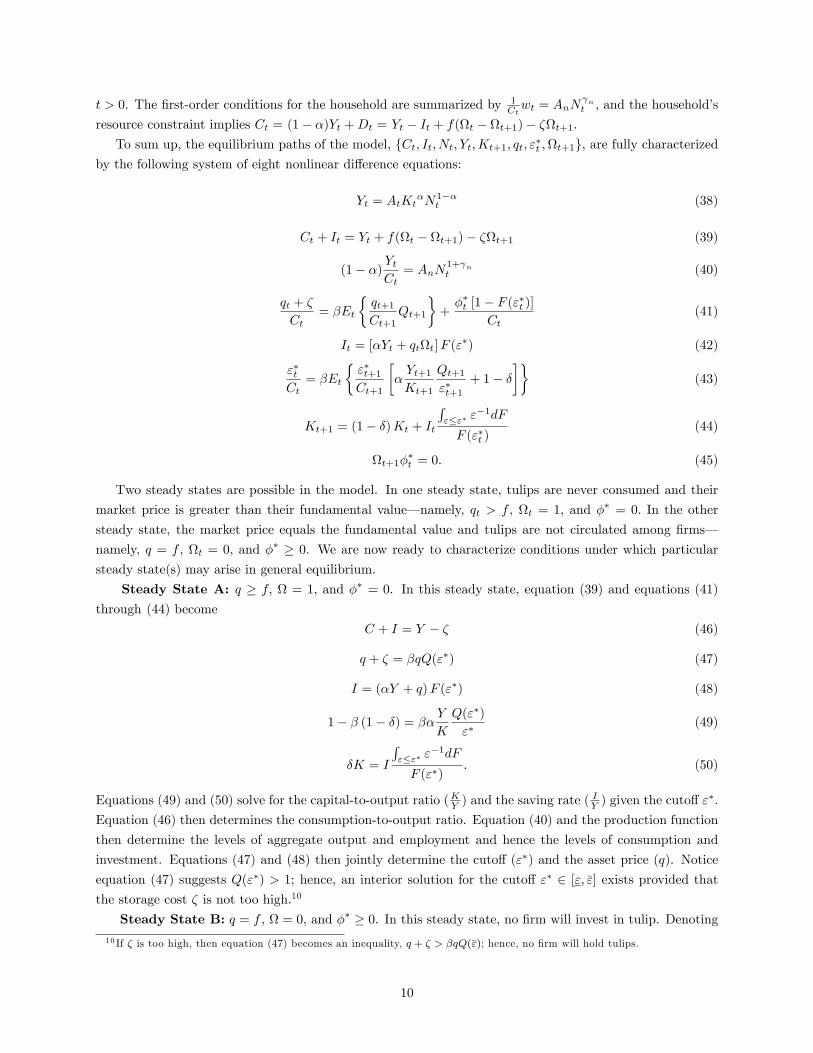
Steady State A: q � f; = 1; and �� = 0. In this steady state, equation (39) and equations (41)
through (44) become
C + I = Y � � (46)
q + � = �qQ("�) (47)
I = (�Y + q)F ("�) (48)
1� � (1� �) = �� YK
Q("�)
"�(49)
�K = I
R"�"� "
�1dF
F ("�): (50)
Equations (49) and (50) solve for the capital-to-output ratio (KY ) and the saving rate (IY ) given the cuto¤ "
�.
Equation (46) then determines the consumption-to-output ratio. Equation (40) and the production function
then determine the levels of aggregate output and employment and hence the levels of consumption and
investment. Equations (47) and (48) then jointly determine the cuto¤ ("�) and the asset price (q). Notice
equation (47) suggests Q("�) > 1; hence, an interior solution for the cuto¤ "� 2 [";�"] exists provided thatthe storage cost � is not too high.10
Steady State B: q = f , = 0, and �� � 0. In this steady state, no �rm will invest in tulip. Denoting
10 If � is too high, then equation (47) becomes an inequality, q + � > �qQ(�"); hence, no �rm will hold tulips.
10
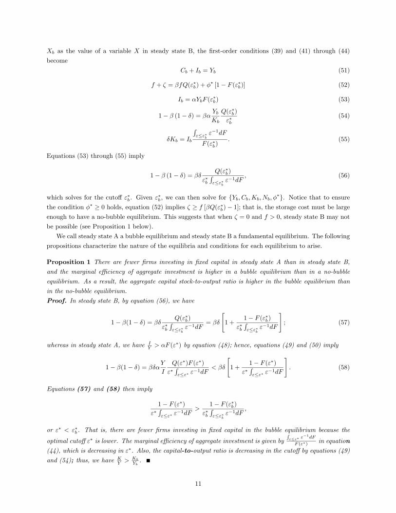
Xb as the value of a variable X in steady state B, the �rst-order conditions (39) and (41) through (44)
become
Cb + Ib = Yb (51)
f + � = �fQ("�b) + �� [1� F ("�b)] (52)
Ib = �YbF ("�b) (53)
1� � (1� �) = �� YbKb
Q("�b)
"�b(54)
�Kb = Ib
R"�"�b
"�1dF
F ("�b): (55)
Equations (53) through (55) imply
1� � (1� �) = �� Q("�b)
"�bR"�"�b
"�1dF; (56)
which solves for the cuto¤ "�b . Given "�b , we can then solve for fYb; Cb;Kb; Nb; �
�g. Notice that to ensurethe condition �� � 0 holds, equation (52) implies � � f [�Q("�b)� 1]; that is, the storage cost must be largeenough to have a no-bubble equilibrium. This suggests that when � = 0 and f > 0, steady state B may not
be possible (see Proposition 1 below).
We call steady state A a bubble equilibrium and steady state B a fundamental equilibrium. The following
propositions characterize the nature of the equilibria and conditions for each equilibrium to arise.
Proposition 1 There are fewer �rms investing in �xed capital in steady state A than in steady state B,
and the marginal e¢ ciency of aggregate investment is higher in a bubble equilibrium than in a no-bubble
equilibrium. As a result, the aggregate capital stock-to-output ratio is higher in the bubble equilibrium than
in the no-bubble equilibrium.
Proof. In steady state B, by equation (56), we have
1� �(1� �) = �� Q("�b)
"�bR"�"�b
"�1dF= ��
"1 +
1� F ("�b)"�bR"�"�b
"�1dF
#; (57)
whereas in steady state A, we have IY > �F ("
�) by equation (48); hence, equations (49) and (50) imply
1� �(1� �) = ���YI
Q("�)F ("�)
"�R"�"� "
�1dF< ��
"1 +
1� F ("�)"�R"�"� "
�1dF
#: (58)
Equations (57) and (58) then imply
1� F ("�)"�R"�"� "
�1dF>
1� F ("�b)"�bR"�"�b
"�1dF;
or "� < "�b . That is, there are fewer �rms investing in �xed capital in the bubble equilibrium because the
optimal cuto¤ "� is lower. The marginal e¢ ciency of aggregate investment is given byR"�"� "
�1dF
F ("�) in equation(44), which is decreasing in "�. Also, the capital-to-output ratio is decreasing in the cuto¤ by equations (49)and (54); thus, we have K
Y > Kb
Yb.
11

Proposition 2 (i) If � = 0 and f = 0, then qt = 0 and �� � 0 for all t is a fundamental equilibrium, andq > 0 and �� = 0 is a possible bubble equilibrium. (ii) If � = 0 and f > 0, then there exists at most one
equilibrium with q � f and �� = 0. (iii) If � > 0 and f � 0, then q = f and �� � 0 is a fundamentalequilibrium; and q > f and �� = 0 is a possible bubble equilibrium.
Proof. We prove the proposition case by case.(i) Suppose � = 0 and f = 0. Then equation (52) is clearly satis�ed if ��t = 0. In such a case, = 0 and
q = 0 is an equilibrium because no �rm has an incentive to deviate by holding tulips when the liquidation
value of a tulip is zero. Hence, a fundamental equilibrium with q = f = 0 exists. To prove the bubble
equilibrium, suppose q > 0. Equation (47) implies Q("�) = 1� , which solves for the cuto¤ value "
� as an
interior point in the support " 2 [";�"] because 1� > 1, provided the upper bound of the support �" is large
enough. Given this, we have 0 < F ("�) < 1. Equation (49) implies the capital-to-output ratio,
K
Y=
�
1� �(1� �)1
"�: (59)
This ratio and equation (50) give the household�s saving rate,
I
Y=
��
1� �(1� �)F
Q� 1 + F ; (60)
where Q� 1+F = "�R"�"� "
�1dF . Equation (48) then implies the asset value-to-output ratio as a function
of the saving rate,q
Y=
�I
Y
1
F ("�)� �
�: (61)
To ensure q > 0 (i.e., qY > 0), we must have I
Y > �F , which implies the following restriction on theparameters:
� >���1 � 1 + F
�(1� � (1� �)) : (62)
That is, if the household is su¢ ciently patient (i.e., � close to 1), then �rms have incentives to hold bubbleswith q > 0; hence, = 1 and �� = 0. (Note that when � is close to 1, Q("�) is also close to 1; hence, "� isclose to its lower bound " and F (") = 0.)
(ii) Suppose � = 0 and f > 0. In this case, q < f is clearly not an equilibrium because the demand
for tulips will increase to in�nity. So let q � f . First, steady state B with q = f , = 0; and �� � 0 is
not an equilibrium. To see this, suppose �rm i deviates from this equilibrium and decides to hold tulips as
a store of value. This makes �rm i�s position better because tulips always have liquidation value f > 0 in
any period and there is no storage cost; hence, tulips help diversify idiosyncratic risk in capital investment
and the demand for tulips will rise. Therefore, all �rms have incentives to deviate and q may rise above
f . Alternatively, by Proposition 1, we have Q("�b) > Q("�) = ��1; then by equation (52), we must have
�� = f(1� �Q("�b))=[1� F ("�b)] < 0, which is contrary to the requirement �� � 0. Thus, steady state B can
never be an equilibrium and we only need to consider steady state A with q � f as a possible equilibrium.In this case, following similar steps in case (i), equation (61) implies that q � f is equivalent to the followingcondition:
��
1� �(1� �)1
��1 � 1 + F� � � f
Y: (63)
There exists a unique equilibrium whenever this condition is satis�ed. For example, condition (63) is satis�ed
when � ! 1.
12
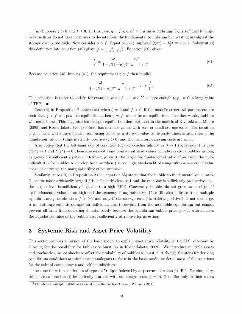
(iii) Suppose � > 0 and f � 0. In this case, q = f and �� � 0 is an equilibrium if � is su¢ ciently large,
because �rms do not have incentives to deviate from the fundamental equilibrium by investing in tulips if the
storage cost is too high. Now consider q > f . Equation (47) implies �Q("�) = q+�q � � > 1. Substituting
this de�nition into equation (49) gives KY = �
1��(1��)�"� . Equation (50) gives
I
Y=
��
1� �(1� �)�F
��1�� 1 + F: (64)
Because equation (48) implies (61), the requirement q > f then implies
��
1� �(1� �)�
��1�� 1 + F� � > f
Y: (65)
This condition is easier to satisfy, for example, when � ! 1 and Y is large enough (e.g., with a large value
of TFP).
Case (ii) in Proposition 2 states that when � = 0 and f > 0; if the model�s structural parameters are
such that q > f is a possible equilibrium, then q = f cannot be an equilibrium. In other words, bubbles
will never burst. This suggests that sunspot equilibrium does not exist in the models of Kiyotaki and Moore
(2008) and Kocherlakota (2009) if land has intrinsic values with zero or small storage costs. The intuition
is that �rms will always bene�t from using tulips as a store of value to diversify idiosyncratic risks if the
liquidation value of tulips is strictly positive (f > 0) and the inventory-carrying costs are small.
Also notice that the left-hand side of condition (63) approaches in�nity as � ! 1 (because in this case
Q("�)! 1 and F ("�)! 0); hence, assets with any positive intrinsic values will always carry bubbles as long
as agents are su¢ ciently patient. However, given �, the larger the fundamental value of an asset, the more
di¢ cult it is for bubbles to develop because when f is too high, the bene�t of using tulips as a store of value
does not outweigh the marginal utility of consumption.
Similarly, case (iii) in Proposition 2 (i.e., equation 65) states that the bubble-to-fundamental value ratio,qf , can be made arbitrarily large if � is su¢ ciently close to 1 and the economy is su¢ ciently productive (i.e.,
the output level is su¢ ciently high due to a high TFP). Conversely, bubbles do not grow on an object if
its fundamental value is too high and the economy is unproductive. Case (iii) also indicates that multiple
equilibria are possible when f > 0 if and only if the storage cost � is strictly positive but not too large.
A mild storage cost discourages an individual �rm to deviate from the no-bubble equilibrium but cannot
prevent all �rms from deviating simultaneously because the equilibrium bubble price q > f , which makes
the liquidation value of the bubble asset su¢ ciently attractive for investing.
3 Systemic Risk and Asset Price Volatility
This section applies a version of the basic model to explain asset price volatility in the U.S. economy by
allowing for the possibility for bubbles to burst (as in Kocherlakota, 2009). We introduce multiple assets
and stochastic sunspot shocks to a¤ect the probability of bubbles to burst.11 Although the steps for deriving
equilibrium conditions are similar and analogous to those in the basic mode, we detail most of the equations
for the sake of completeness and self-containedness.
Assume there is a continuum of types of "tulips" indexed by a spectrum of colors j 2 R+. For simplicity,
tulips are assumed to (i) be perfectly storable with no storage costs (� = 0), (ii) di¤er only in their colors
11The idea of multiple bubble assets is akin to that in Kareken and Wallace (1981).
13

(types), and (iii) have no intrinsic values (f = 0).12 Thus, according to Proposition 2, each type of tulip
asset can be a bubble with the following property: Its equilibrium price is zero if no �rms in the economy
expect other �rms to invest in it, and the price is strictly positive if all agents expect others to hold it.
In each period a constant measure z of new colors of tulips is born (issued).13 The supply of each color
(variety) of tulips is normalized to 1; hence, each tulip has a unique color. Also, all tulips have the same
probability, pt; to lose their values in each period regardless of color. This assumption captures the concept
of systemic risk. The newborn tulips are distributed equally to all agents (�rms) as endowments, and issuing
(producing) new tulips does not cost any social resources. Let qjt denote the price of a tulip (with color) j
and hjt+1(i) the quantity of the tulip j demanded by �rm i 2 [0; 1]. The aggregate number (stock) of tulipsevolves over time according to the law of motion:
t+1 = (1� pt)t + z; (66)
where is the measure of the stock of tulips in the entire economy. The market clearing condition for each
tulip with color j is Z 1
i=0
hjt+1(i)di = 1: (67)
As in the basic model, �rms have the same constant returns to scale production technologies and are hit
by idiosyncratic cost shocks to the marginal e¢ ciency of investment "(i). A �rm�s problem is to determine
a portfolio of tulips to maximize discounted future dividends. Its resource constraint is
dt(i) + it(i) +
Zj2t+1
qjthjt+1(i)dj + wtnt(i) � Atkt(i)�nt(i)1�� +
Zj2t
qjthjt (i)1
jtdj +
Zj2z
qjtdj; (68)
where w is the real wage, is the set of available colors of tulips, and the index variable 1jt satis�es
1jt =
8><>:1 with prob. 1� pt
0 with prob. pt
: (69)
Namely, each tulip bought in period t� 1 may lose its value completely with probability pt in the beginningof period t. As in the basic model, we impose the following constraints: it(i) � 0, dt(i) � 0, and hjt+1(i) � 0for all j 2 .Using the same de�nition of R as in the basic model, the �rm�s problem is to solve
maxE0
1Xt=0
�t�t
"Rtkt(i)� it(i) +
Zj2t
qjthjt (i)1
jtdj +
Zj2z
qjtdj �Zj2t+1
qjthjt+1(i)dj
#; (70)
subject to
dt(i) � 0 (71)
hjt+1(i) � 0 for all j (72)
it(i) � 0 (73)
12These assumptions reduce the number of parameters and simplify our calibration analysis.13We can also allow z to be stochastic.
14

kt+1(i) = (1� �) kt(i) +it(i)
"t(i): (74)
Letn�(i); �jt (i); �(i); �(i)
odenote the Lagrangian multipliers of constraints (71) through (73), respectively,
the �rst-order conditions fornit(i); kt+1(i); h
jt+1(i)
oare similar to those in the basic model and denoted,
respectively, by
1 + �t(i) =�t(i)
"t(i)+ �t(i) (75)
�t(i) = �Et�t+1�t
�[1 + �t+1(i)]Rt+1 + (1� �)�t+1(i)
(76)
[1 + �t(i)] qjt = �Et
�t+1�t
nqjt+11
jt+1
�1 + �t+1(i)
�o+ �jt (i); (77)
plus the complementary slackness conditions,
�t(i)it(i) = 0 (78)
�jt (i)hjt+1(i) = 0 for all j (79)
[1 + �t(i)]
"Rtkt(i)� it(i) +
Zj2t
qjthjt (i)1
jtdj +
Zj2z
qjtdj �Zj2t+1
qjthjt+1(i)dj
#= 0: (80)
3.1 Decision Rules
As in the basic model, the decision rules at the �rm level are characterized by a cuto¤ strategy. The following
steps are analogous to those in the basic model. Consider two possibilities:
Case A: "t(i) � "�t . In this case, the cost of capital investment is low. Suppose it(i) > 0; accordinglywe have �t(i) = 0. Equations (75) and (76) imply
"t(i) [1 + �t(i)] = �Et�t+1�t
�[1 + �t+1(i)]Rt+1 + (1� �)�t+1(i)
: (81)
Given that �t(i) � 0, we must have "t(i) � �Et�t+1�t
�[1 + �t+1(i)]Rt+1 + (1� �)�t+1(i)
, which de�nes the
cuto¤ value, "�t :
"�t � �Et�t+1�t
�[1 + �t+1(i)]Rt+1 + (1� �)�t+1(i)
: (82)
Equation (75) then becomes 1+�t(i) ="�t"t(i)
. Hence, whenever "t(i) < "�t , we must have �t(i) ="�t"t(i)
�1 > 0and dt(i) = 0. Equation (77) becomes
"�t"t(i)
qjt = �Et�t+1�t
nqjt+11
jt+1
�1 + �t+1(i)
�o+ �jt (i): (83)
De�ning ��t as the cuto¤ value of �jt (i) for �rms with "t(i) = "
�t , equation (84) implies
qjt = �Et�t+1�t
nqjt+11
jt+1
�1 + �t+1(i)
�o+ ��t (84)
Given that ��t � 0, the fact that �jt (i) > �
�t under Case A yields �
jt (i) > 0. That is, for any "t(i) < "
�t , we
must have hjt+1(i) = 0 for all j 2 t+1 and it(i) = Rtkt(i) +Rj2t q
jthjt (i)1
jtdj +
Rj2z q
jtdj. This suggests
15

that �rms opt to liquidate all tulip assets to maximize investment in �xed capital when the cost of �xed
investment is low.
Case B: "t(i) > "�t . In this case, the cost of investing in �xed capital is high. Suppose dt(i) > 0 and
�t(i) = 0. Then equations (75) and (76) and the de�nition of the cuto¤ "� imply �t(i) = 1� "�t
"t(i)> 0. Hence,
we have it(i) = 0. In such a case, �rms opt not to invest in �xed capital and, instead, pay the shareholders
a positive dividend. Because the market clearing condition for each tulip j isRhjt+1(i)di = 1, we must also
have hjt+1(i) > 0 and �jt (i) = 0 for all j 2 t+1 under Case B. Thus, equations (77) and (84) then imply the
cuto¤ ��t = 0.
Combining these two cases, the decision rule for capital investment is given by
it(i) =
8><>:Rtkt(i) +
Rj2t q
jthjt (i)1
jtdj +
Rj2z q
jtdj if "t(i) � "�t
0 if "t(i) > "�t
: (85)
The option value of liquidity is again de�ned by Q � E [1 + �(i)] =Rmax
n1; "
�
"(i)
odF ("). Using equations
(83) and (84), the Lagrangian multiplier for the nonnegativity constraint (72) is given by
�jt (i) =
8>><>>:�"�
"(i) � 1�qjt if "(i) � "�
0 if "(i) > "�; (86)
and the average shadow value of �j isR�j(i)di = qj
R"�"�
�"�
" � 1�dF (") = qj (Q� 1), which is independent
of i but proportional to the tulip�s price, qj .Integrating equation (77) over i and rearranging gives
qjt = �Et�t+1�t
qjt+11jt+1Qt+1; (87)
where the right-hand side is the expected rate of return to tulip j. This equation shows that if pt = 1 (i.e.,
1jt = 0 with probability 1), then tulip j�s equilibrium price is given by qjt = 0 for all t because the demand
for such an asset is zero when it has no market value in the next period. More importantly, even if p < 1
(e.g., p = 0), qjt = 0 for all t is still an equilibrium because no �rms will hold tulip j if they do not expect
others to hold it. In the next section, we de�ne restrictions on the value of p so that qjt > 0 constitutes a
bubble equilibrium.
3.2 Aggregation and General Equilibrium
As in the basic model, we have at the aggregate level Nt =h(1��)At
wt
i 1�
Kt, Yt = At
h(1��)At
wt
i 1���
Kt,
Yt = AtK�t N
1��t , wt = (1� �) YtNt
, and Rt = � YtKt. Consider a symmetric equilibrium14 where
qjt1jt =
8><>:qt with prob. 1� pt
0 with prob. pt
; (88)
14A symmetric equilibrium exists because of arbitrage across tulips of di¤erent colors.
16
where qt is the price of tulips of all colors. De�ne xt(i) �Rj2t q
jthjt (i)1
jtdj +
Rj2z q
jtdj and Xt �
R 10x(i)di.
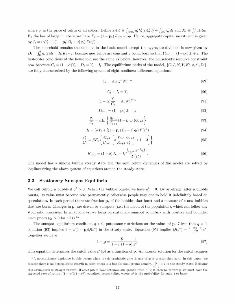
By the law of large numbers, we have Xt = (1� pt) tqt+ zqt. Hence, aggregate capital investment is givenby It = (�Yt + [(1� pt) t + z] qt)F ("�t ).The household remains the same as in the basic model except the aggregate dividend is now given by
Dt =R 10dt(i)di = RtKt�It because new tulips are constantly being born so that t+1 = (1�pt)t+z. The
�rst-order conditions of the household are the same as before; however, the household�s resource constraint
now becomes Ct = (1� �)Yt +Dt = Yt � It. The equilibrium paths of the model, fC; I;N; Y;K 0; q; "�;0g,are fully characterized by the following system of eight nonlinear di¤erence equations:
Yt = AtKt�N1��
t (89)
Ct + It = Yt (90)
(1� �) YtCt= AnN
1+ nt (91)
t+1 = (1� pt)t + z (92)
qtCt= �Et
�qt+1Ct+1
(1� pt+1)Qt+1�
(93)
It = (�Yt + [(1� pt)t + z] qt)F ("�) (94)
"�tCt= �Et
�"�t+1Ct+1
��Yt+1Kt+1
Qt+1"�t+1
+ 1� ���
(95)
Kt+1 = (1� �)Kt + It
R"�"� "
�1dF
F ("�t ): (96)
The model has a unique bubble steady state and the equilibrium dynamics of the model are solved by
log-linearizing the above system of equations around the steady state.
3.3 Stationary Sunspot Equilibria
We call tulip j a bubble if qjt > 0. When the bubble bursts, we have qjt = 0. By arbitrage, after a bubble
bursts, its value must become zero permanently, otherwise people may opt to hold it inde�nitely based on
speculation. In each period there are fraction pt of the bubbles that burst and a measure of z new bubblesthat are born. Changes in pt are driven by sunspots (i.e., the mood of the population), which can follow any
stochastic processes. In what follows, we focus on stationary sunspot equilibria with positive and bounded
asset prices (qt > 0 for all t).15
The sunspot equilibrium condition, q > 0, puts some restrictions on the values of p. Given that q > 0,
equation (93) implies 1 = �(1 � p)Q("�) in the steady state. Equation (95) implies Q("�) = 1��(1��)�R "�.
Together we have
1� p = R
1� � (1� �)1
"�: (97)
This equation determines the cuto¤ value "�(p) as a function of p. An interior solution for the cuto¤ requires
15A nonstationary explosive bubble occurs when the deterministic growth rate of qt is greater than zero. In this paper, we
assume there is no deterministic growth in asset prices in a bubble equilibrium; namely,qjt
qjt�1
= 1 in the steady state. Relaxing
this assumption is straightforward. If asset prices have deterministic growth rates rj � 0, then by arbitrage we must have theexpected rate of return, (1� �j)(1 + rj), equalized across tulips, where �j is the probability for tulip j to burst.
17

"�(p) 2 (";�"), where ";�" > 0 are the lower and upper bounds of the support for "t(i), respectively. Hence,we must have
R
1� � (1� �)1
"> (1� p) > R
1� � (1� �)1
�": (98)
Notice that R1��(1��) =
P1j=0 �
j (1� �)j � YK is the present value of the marginal products of capital and 1"
is the marginal e¢ ciency of investment. Hence, the conditions in equation (98) state that the real expected
rate of return to tulips (i.e., the survival probability of a speculative bubble) must be comparable to that of
capital investment (Tobin�s q) to induce people to hold both capital and bubbles.The wider the support of the idiosyncratic shocks, the larger the permissible region for the value of p.
This simply restates the �nding that idiosyncratic uncertainty in the expected rate of returns to capital
investment (or Tobin�s q) is the fundamental reason for people to invest in bubbles. When such idiosyncratic
assessments of risks converge (e.g., " = �"), it is virtually impossible for bubbles to arise (i.e., the measure of
sunspot equilibria becomes zero).
In the steady state, equations (93) through (96) become
1 = �(1� p)Q("�) (99)
I = (�Y +q)F ("�) (100)
1� � (1� �) = �� YK
Q("�)
"�(101)
�K = I
R"�"� "
�1dF
F ("�): (102)
Equation (99) solves for the cuto¤ value "�. Equation (101) implies the capital-to-output ratio, KY =
��1��(1��)
Q"� . Equations (102) and (101) give the household�s saving rate, I
Y = ���1��(1��)
FQQ�1+F , where
Q � 1 + F = "�R"�"� "
�1dF . Equation (100) implies the asset-to-output ratio as a function of the saving
rate, qY = 1F ("�)
IY � �. As in the basic model, to ensure
qY > 0, we must have I
Y > �F , which implies
� >���1 � 1 + F
�(1� � (1� �)).
3.4 Calibration and Impulse Responses
Assume that "(i) follows the Pareto distribution, F (") = 1 � "��, with the shape parameter � = 1:5 and
the support (1;1).16 With this distribution, we have Q = �1+� "
�+ 11+� "
���. We normalize the steady-state
values z = 1 and A = 1 and calibrate the structural parameters of the model as follows: The time period isa quarter, the capital�s income share � = 0:4, the time-discounting factor � = 0:99, the capital depreciation
rate � = 0:025, and the inverse elasticity of labor supply n = 0 (indivisible labor).
The driving processes of the model are assumed to follow AR(1) processes,
lnpt = �p lnpt�1 + (1� �p) ln �p+ "pt (103)
lnAt = �A lnAt�1 + "At; (104)
where the steady-state probability for bubbles to burst is set to �p = 0:1. To show the potential of the model
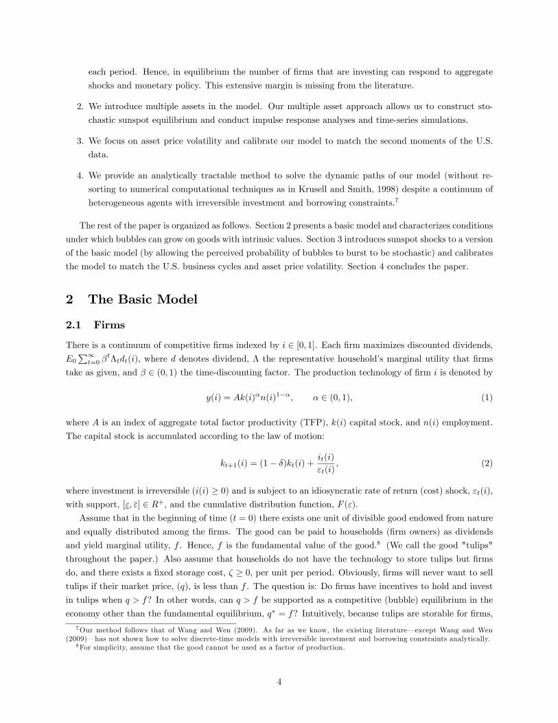
in explaining asset price volatility, Figure 2 plots the impulse responses of the output and tulip price to a
16The results are not sensitive to the values of �. For example, with � = 3 we obtain similar results.
18

1 percent decrease in productivity "At and compares them with a 10 percent increase in the probability for
bubbles to burst. A positive shock to "p is akin to a �nancial crisis because it implies a higher systemic
�nancial risk. We set �p = �A = 0:9 in the impulse responses.
Figure 2. Impulse reponses to probably shock (top windows) and productivity shock (bottom windows).
The top windows in Figure 2 show that an increase in the bubbles� probability to burst generates a
recession in aggregate output (upper-left window) and a dramatic drop in asset prices (upper-right window).
When the perceived rate of return to tulips decreases (or the �nancial risk increases), agents rationally
decrease their demand for tulips, leading to a sharp fall in asset price. Because tulip assets provide liquidity
for �rms, "panic" sales of tulips reduce �rms�net worth and working capital, leading to a U-shaped decline
in output, employment, and capital investment. Such a hump-shaped output dynamics suggest that asset
price movements lead the business cycle and provide a key litmus test of business cycle models (see Cogley
and Nason, 1995). Our model passes this test with �ying colors in this dimension. More importantly, asset
prices are far more volatile than the fundamentals. For example, the initial drop in asset prices is more than
32 times larger than that in output, resembling a typical stock market crash. In contrast, an adverse shock
to aggregate productivity generates a fall in asset prices (lower-right window) that is only twice as large as
the fall in output (lower-left window). Hence, to understand the excessive asset market volatilities, shocks
to the probability of the burst of asset bubbles (i.e., systemic �nancial risk) are essential.
To test whether the model has the potential to match the U.S. time-series data quantitatively, we calibratethe two driving processes fAt;ptg using the Solow residuals and the S&P 500 price index (normalized by
19

the GDP de�ator) from the U.S. economy (1947:1�2009:1), respectively. For each time series, we apply
the Hodrick-Prescott �lter on the logged series and estimate an univariate AR(1) model to obtain the
coe¢ cients��p; �A
. The covariance matrix of the two residuals from the AR(1) models is then used
to calibrate f"pt; "Atg. The results are as follows: �p = 0:85; �A = 0:75; �"p = 0:056; �"A = 0:00625;
and corr("p; "A) = �0:3. A negative correlation suggests that it is less likely for bubbles to burst when
productivity is high. The data show that the innovations in stock prices are about 9 times more volatile
than the innovations in productivity. Based on these values, we reset �p = 0:15 so that the implied relative
volatility of asset price to output is in line with the data. We generate 10; 000 observations from the model
and estimate the model�s moments. Given the large sample size, the standard errors are small and they are
thus not reported. Table 1 reports the predicted second moments of the model and their counterparts in the
data.17
Table 1. Selected Second Moments
std �x relative std �x�y
corr(x; y) corr(xt; xt�1)
x y c i n q c i n q c i n q y c i n q
Data :017 :010 :050 :016 :099 :60 2:98 :98 5:93 :78 :77 :83 :46 :83 :81 :84 :90 :80
Model :012 :009 :025 :005 :068 :74 2:12 :42 5:76 :93 :92 :75 :35 :79 :83 :80 :83 :80
According to the table, the model�s predictions are broadly consistent with the U.S. data. For example,
in terms of standard deviations, the model is able to explain about 70 percent of output �uctuations and
70 percent of stock price movements in the data. In terms of relative volatilities with respect to output, the
model predicts that consumption is about 25 percent less volatile, investment about 2 times more volatile,
and asset price nearly 6 times more volatile than output; these predictions are broadly consistent with the
U.S. economy. In the data, the correlation between stock prices and output at the business cycle frequencies
is 0:46; this value is 0:35 in the model, qualitatively matching the data. The model also can generate strong
autocorrelations in output, consumption, investment, labor, and asset prices that are very close to the data.
The gap between model and data is most signi�cant in the relative volatility of employment to output; the
model signi�cantly underestimated the volatility of employment even with indivisible labor.
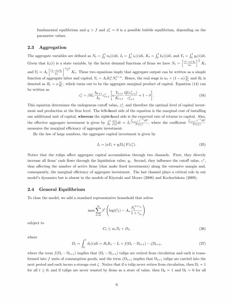
We can simulate a tulip bubble using the model. For example, assuming the time period to be a quarter
and letting the probability of bubble to burst follow a moving average process,
pt = �p+T�1Xj=0
�j"t�j ;
where " is zero mean i.i.d. innovations. Suppose T = 8, �p = 0:1, and the probability weight vector
� = 1100 [1; 2; 1; 1; 0;�1;�1;�2]. The simulated tulip bubble is graphed in Figure 3. The larger the value
of �p, the larger the bubble will be. The vector � has zero mean and determines the shape of the bubble.The intuition behind the values of � is as follows: Because agents are forward looking, they react to good
�nancial news by buying tulips now when they perceive that the probability of the bubbles to burst willbe lower several periods from now. Thus, tulip prices would increase immediately. To prevent a big jump
in the current tulip prices, there must be enough bad news today so that investors are cautious in entering
the tulip market. This is why � takes positive values initially so that the bubble only grows slowly and
gradually.17The data are quarterly and include real GDP (y), nondurable goods consumption (c), total �xed investment (i), total
private employment by establishment survey, and the S&P 500 price index normalized by the GDP de�ator. The sample coversthe period 1947:1�2009:1.
20

Figure 3. Simulated tulip bubble.
4 Conclusion
This paper provides an in�nite-horizon DSGE model with heterogeneous agents to explain asset price volatil-
ity. It characterizes conditions under which bubbles with market values exceeding their fundamental values
may arise. It is shown that rational agents are willing to invest in such bubbles despite their positive prob-
ability to burst and that changes in the perceived systemic risk in the asset market can trigger boom-bust
cycles and asset price collapse. Calibration exercises con�rm that the model has the potential to quanti-
tatively explain the U.S. business cycle and asset price volatility. As potential research topics, it would be
interesting to consider welfare analysis and optimal policies in a bubble economy as in Kiyotaki and Moore
(2008) and Kocherlakota (2009) and to consider bubbles with nonstationary prices. We leave these issues to
future research.
21

References
[1] Angeletos, G.-M., 2007, Uninsured idiosyncratic investment risk and aggregate saving, Review of Eco-
nomic Dynamics 10(1), 1-30.
[2] Araujo, A., Pascoa, M., and Torres-Martinez, J., 2005, Bubbles, collateral, and monetary equilibrium,
PUC-Rio Working Paper No. 513.
[3] Azariadis, C., 1981. Self-ful�lling prophecies, Journal of Economic Theory 25(3), 380-396.
[4] Benhabib, J., and Farmer, Roger., 1994, Indeterminacy and increasing returns, Journal of Economic
Theory 63(1), 19-41.
[5] Bewley, T., 1980, "The optimum quantity of money," in Models of Monetary Economics, ed. by John
Kareken and Neil Wallace. Minneapolis, Minnesota: Federal Reserve Bank, 1980.
[6] Caballero, R., and Krishnamurthy, A., 2006, Bubbles and capital �ow volatility: Causes and risk
management, Journal of Monetary Economics 53(1), 35-53.
[7] Cass, D. and K. Shell, 1983, Do sunspots matter? Journal of Political Economy 91(2), 193�227.
[8] Cogley, T., Nason, J., 1995. Output dynamics in real-business-cycle models, American Economic Review85(3), 492�511.
[9] Dash, Mike (1999), Tulipomania: The Story of the World�s Most Coveted Flower and the Extraordinary
Passions It Aroused. London: Gollancz.
[10] Farhi, E. and J. Tirole, 2008, Competing Liquidities: Corporate Securities, Real Bonds and Bubbles,
NBER Working Paper No. W13955.
[11] Garber, Peter M., 1989, "Tulipmania," Journal of Political Economy 97 (3): 535�560.
[12] Garber, Peter M., 1990, "Famous �rst bubbles," Journal of Economic Perspectives 4 (2): 35�54.
[13] Hellwig, C., and Lorenzoni, G., 2009, Bubbles and self-enforcing debt, Econometrica (forthcoming).
[14] Kiyotaki, N., and Moore, J., 2008, Liquidity, business cycles, and monetary policy, Princeton University
working paper.
[15] Kocherlakota, N., 1992, Bubbles and constraints on debt accumulation, Journal of Economic Theory
57(1), 245-256.
[16] Kocherlakota, N., 2009, Bursting bubbles: Consequences and cures, University of Minnesota working
paper.
[17] Krusell, P., and Smith A., 1998, Income and wealth heterogeneity in the macroeconomy, Journal of
Political Economy 106(5), 867-896.
[18] Mackay, Charles, 1841, Memoirs of Extraordinary Popular Delusions and the Madness of Crowds, Lon-
don: Richard Bentley. Republished as Extraordinary Popular Delusions and the Madness of Crowds,
Hampshire, UK: Harriman House, 2003.
22

[19] Samuelson, P., 1958. An exact consumption-loan model of interest with or without the social contrivance
of money, Journal of Political Economy 66(6), 467�482.
[20] Santos, M., and Woodford, M., 1997, Rational asset pricing bubbles, Econometrica 65(1), 19-57.
[21] Scheinkman, J., and Weiss, L., 1986, Borrowing constraints and aggregate economic activity, Econo-
metrica 54(1), 23-46.
[22] Thompson, Earl (2007), "The tulipmania: Fact or artifact?" Public Choice 130(1): 99�114.
[23] Tirole, J., 1985, Asset bubbles and overlapping generations, Econometrica 53(6), 1499-1528.
[24] Wang, P. and Y. Wen, 2007, Incomplete information and self-ful�lling prophecies, Federal Reserve Bank
of St. Louis Working Paper No. 2007-033B.
[25] Wang, P. and Y. Wen, 2008, Imperfect competition and indeterminacy of aggregate output, Journal of
Economic Theory 143(1), 519-540.
[26] Wang, P. and Y. Wen, 2009, Financial development and economic volatility: A uni�ed explanation,
Federal Reserve Bank of St. Louis Working Paper No. 2009-022C.
[27] Wen, Y., 2009, Liquidity and welfare in a heterogeneous-agent economy, Federal Reserve Bank of St.
Louis Working Paper No. 2009-019B.
[28] Woodford, M., (1986), Stationary sunspot equilibria in a �nance-constrained economy, Journal of Eco-
nomic Theory 40(1), 128-137.
23