spectrum map and its application in resource management in

406 IEEE TRANSACTIONS ON COGNITIVE COMMUNICATIONS AND NETWORKING, VOL. 1, NO. 4, DECEMBER 2015

Spectrum Map and Its Application in ResourceManagement in Cognitive Radio Networks

Saptarshi Debroy, Shameek Bhattacharjee, and Mainak Chatterjee

Abstract—Measurements on radio spectrum usage haverevealed an abundance of under-utilized bands of spectrum thatbelong to primary (licensed) networks. Prior knowledge aboutthe occupancy of such bands and the expected achievable perfor-mance on those bands can help secondary (unlicensed) networksto devise effective strategies to improve utilization. Such priorspatio-temporal spectrum usage statistics can either be obtainedfrom a database that is maintained by the primary networks orcould be measured by customized sensors deployed by the sec-ondary networks. In this paper, we use Shepard’s interpolationtechnique to estimate a spatial distribution of spectrum usageover a region of interest, which we call the spectrum map. Theinterpolation is achieved by intelligently fusing the data sharedby the the secondary nodes considering their mutual distancesand spatial orientation with each other. The obtained map is atwo-dimensional (2-D) interpolation function that is continuouslydifferentiable and passes through all the spectrum usage valuesrecorded at arbitrary locations; thus providing a reference forprimary occupancy in that region. For determining the optimallocations for sensing primary activity, we use an iterative cluster-ing technique that uses tree structured vector quantization. We usethe spectrum map to estimate different radio and network per-formance metrics like channel capacity, network throughput, andspectral efficiency. As a comprehensive case study, we demonstratehow the spectrum map can be used for efficient resource allocationin TV white space. In particular, we consider an IEEE 802.22-based WRAN and show how the rendezvous probability can beimproved for better radio resource allocation, thereby increasingthe secondary spectrum utilization.

Index Terms—Cognitive Radio Network, Spectrum Map,Cooperative Spectrum Sensing, Resource Allocation, IEEE 802.22WRAN.

I. INTRODUCTION

I N a cognitive radio network (CRN), secondary nodes (i.e.,unlicensed users) equipped with cognitive radio enabled

devices continuously monitor the presence of primary (i.e.,licensed) nodes and opportunistically access the unused orunder-utilized licensed bands of primaries [1]. However, themost important regulatory aspect of these networks is the factthat the secondary nodes must not interfere with primary trans-missions. Thus, when secondary nodes detect transmissions

Manuscript received January 30, 2015; revised November 4, 2015;accepted December 12, 2015. Date of publication January 12, 2016; date ofcurrent version June 14, 2016. The associate editor coordinating the review ofthis paper and approving it for publication was A. B. MacKenzie.

S. Debroy is with the Department of Computer Science, University ofMissouri, Columbia, MO 65211 USA (e-mail: [email protected]).

S. Bhattacharjee is with the Department of Computer Science, MissouriUniversity of Science and Technology, Rolla, MO 65409 USA (e-mail:[email protected]).

M Chatterjee is with the Department of Electrical Engineering and ComputerScience, University of Central Florida, Orlando, FL 32816 USA (e-mail:[email protected]).

Digital Object Identifier 10.1109/TCCN.2016.2517001

from primaries, they are mandated to relinquish those interfer-ing channels immediately and switch to other non-interferingchannels. Due to the temporal and spatial fleetingness of pri-mary spectrum occupancy, such reactive nature of secondarynetworks is insufficient for desired utilization of under-usedlicensed spectrum. However, a prior knowledge of the possibletransmission activities of the primaries can allow the secondarynodes to effectively access the available channels and predictthe expected radio and network performances for quality of ser-vice (QoS) provisioning. Thus, there is a need to proactivelyestimate the spectrum usage at any arbitrary location and pre-dict the nature of spectrum utilization in the region of interest.In order to facilitate such preemptive primary usage knowledgeacquisition, the recent ruling by FCC [2] necessitates the needfor networks to create, manage, and refer to spectrum databasesfor efficient secondary access without providing any concreteframework. This has opened new discussions on the design,implementation techniques and capabilities of such spectrumdatabases.

Spectrum databases are usually manifested either throughmandating primary transmitters to report their transmissionactivities to a central authority, or through building spectrumusage maps (e.g., TV whitespace database [3]). Spectrum usagemaps give signal strength from primary transmitters on differ-ent channels in a particular geographical region. The stringentpolicy enforcement of reporting spectrum activities has hadsome roadblocks in terms of the underlying legal and policyissues, which are suspected to pose a barrier for wide-adoptionof dynamic spectrum access technologies. Thus, primary usageprediction schemes and models have garnered much tractionin recent times. These schemes mostly deal with either mod-eling spectrum utilization using statistical models [4] or usingreal-world measurement data to predict usage patterns [5]. Suchmechanisms are mostly specific to primary network types (suchas, TV, cellular etc.) and lack extensibility for generic primarynetworks. Thus, structuring design principles and implemen-tation specifics for predicting spectrum usage at any arbitrarylocation for any generic primary network still remains a chal-lenge. This work is motivated by the idea of radio frequency(RF) cartography, which suggests developing a map of theRF field in space by sampling this field at particular loca-tions, which could be done by receivers or dedicated RFsensors. These samples are then interpolated or extrapolated toyield an estimate of the RF field at every point in the space.Although our work is independent of the underlying primarynetworks and secondary sensor devices, our solutions do con-sider their applicability to solve practical secondary networkingproblems.

2332-7731 © 2016 IEEE. Personal use is permitted, but republication/redistribution requires IEEE permission.See http://www.ieee.org/publications_standards/publications/rights/index.html for more information.

DEBROY et al.: SPECTRUM MAP AND ITS APPLICATION IN RESOURCE MANAGEMENT 407

In this paper, we create a spectrum map by defining aspatial distribution function for spectrum utilization. This mapworks as a reference database to predict the spectrum usageat any arbitrary location. We argue that such prediction canbe achieved by fusing the information gathered by the vari-ous stationary secondary nodes operating at different locations.Therefore, we use a collection of such nodes at different loca-tions that monitor the spectrum usage in a distributed mannerand share their findings with others. By fusing the raw spectrumusage data from these nodes, we show how an interpolationfunction can be used to construct a continuously differen-tiable distribution function which governs the estimation of thespectrum utilization at any location. The proposed scheme isindependent of the outdoor fading and shadowing environment;only the sampling and reporting frequencies may vary depend-ing on the environment. To find optimal locations for thesemonitoring nodes, we use an iterative clustering techniqueusing tree structured vector quantization (TSVQ).

We evaluate our proposition by measuring the accuracy ofestimation and also characterizing the nature of the spectrummap. We emulate an environment using the real-world spectrumdata of RWTH Mobnets [6] and replicating their transmissionpattern. We observe that the projected spectrum map mimicsthe real nature of spectral power density. We also demonstratethe effectiveness of iterative clustering in finding the sensinglocations over random selection through simulation experi-ments. We use the prior knowledge of spectrum utilization topredict radio and network performance. We demonstrate howperformance metrics like the channel capacity, spectrum effi-ciency, and system throughput, can be estimated for a secondarytransmitter-receiver pair at any secondary network location. Wealso simulate the nature of these performance metrics.

We also apply our spectrum map for a secondary network usecase: intra-cell channel allocation for IEEE 802.22 networks[7], [8] in TV white space. We show how using spectrum map,the rendezvous probability between secondary users increasesin the absence of a common control cannel. Our spectrum mapinspired channel allocation algorithm achieves close to perfectallocation and more than 50% utilization of free channels evenin the worst case scenario with no intra-cell spatial reuse.

The rest of the paper is organized as follows. In Section II,we discuss the notable prior work in this area. In Section III,we show how the spectrum map is built with data obtainedfrom arbitrary sensing locations. In Section IV, we use describethe iterative clustering technique for finding the ideal sens-ing locations. In Section V, spectrum map-aided predictionof performances metrics are discussed. In Section VI, wepresent the IEEE 802.22 network channel allocation case study.Conclusions are drawn in the last section.

II. RELATED WORK

Prior work in modeling the spectrum usage involves derivingthe distribution of spectrum utilization in a primary networkusing both theoretical models and real-world data logs [4], [5],[6], [9], [10], [11], [12]. One of the earliest work in spectrummeasurements was reported by NSF [9] where it was con-cluded that less than 1% of the spectrum opportunities, both in

frequency and time, were utilized at the place of measurement.Authors in [5] measured the spectrum usage at different loca-tions in Tokyo city and created 3-dimensional plots that showedthe temporal distribution of frequency usage near the monitoredpoints. In [4], the authors observed that the location distribu-tion of primary TV transmitters in USA and Europe closelyfollow the Poisson model. A frequency distribution model toemulate the nature of noise from a primary transmitter on dif-ferent channels was presented in [6]. The most notable studywas carried out by Harrold et. al [10] where three years ofcontinuous measurements for the city of Chicago were pre-sented. Some notable work has also been done on geolocationdatabases. Authors in [13] highlight the benefits of geoloca-tion database technology and Murty et. al in [14] went closestto implementing a database-driven secondary network for TVwhite space (TVWS).

Although most of the above real-world data based learningschemes have valid contribution in the area of primary usageestimation, as with most learning algorithms, there is a ‘time tolearn’. On a macro time scale where events occur on large timedurations (e.g., limited spectrum utilization during weekendsin a downtown area), such learning helps. However, researchhas shown that in order to capture the instantaneous spectrumoccupancy coupled with the channel fading conditions and usethat for scheduling at the MAC layer every 10 or 20 ms (4G net-works), learning does not yield optimal results. Moreover, someof the primary traffic has been proven to obey Poisson distribu-tion [15], [16]; making learning ineffective in such cases. Thus,decisions based on the ground truth obtained by the sensors areproving to be more effective.

Works based on such ground truth observation mostly pro-pose interpolation or extrapolation functions that estimate newdata points given a discrete set of observed data points. Themost common in this category are linear, piece-wise linear,polynomial, splines, multi-variant, Whittaker-Shannon, nearestneighbor, and Hermite interpolation based techniques. As far asconstructing spectrum maps using interpolation are concerned,there have been a few notable efforts. In [17], a spline basedmethod for field estimation was introduced that uses collabora-tive and adaptive sensing. In [18], an algorithm was developedfor sensor placement on a map that is generated by Kriging andLiVE techniques. In [19], a linear unbiased predictor was devel-oped to predict the value at any point on the map’s surface.The reliability of the bounds of interpolation techniques thatare inverse distance weighting based were analyzed in [20].

Although the above mentioned techniques allow predictionof spectrum usage at unknown locations, there is still littleunderstanding on how to build a mathematical function thatcaptures the spatial distribution for the spectrum utiliza-tion. Moreover, for these techniques, construction of a newdata point from known ones is computationally intensive.Sometimes, convergence is slow for techniques that resortto numerical methods. For example, the Kriging method andits variants are among the most popular methods. However,the basic Kriging approaches suffer from poor scalability,requiring up to O(n3) operations for prediction at a singlelocation, where n is the number of measurement points fromwhich data is obtained [21]. Furthermore, the success of most


of these proposed interpolation algorithms is restricted byweaker power levels as the efficiency of the interpolationscheme is a function of received signal strength. Thus, suchschemes have limitations of their applicability for differenttypes of primary networks. Therefore, there is a requirementfor a generic spectrum usage estimation technique that iscomputationally lightweight and equally efficient for differenttypes of primary networks (e.g., TVWS, cellular network, 4Getc.) with different transmission characteristics.

III. BUILDING THE SPECTRUM MAP

The basis for modeling a spatial distribution of spectrumusage is to estimate the activity on every channel. Such esti-mation of spectrum usage at any arbitrary point from a givenset of points is non-trivial. In essence, we seek to define a con-tinuously differentiable two-dimensional interpolation functionwhich passes through all the given irregularly-spaced datapoints1. It can be noted that the estimation method is identicalfor both distributed and centralized sharing system.

A. Sharing Raw Spectrum Data

The concept of sharing and fusing spectrum data amongcognitive radio enabled devices is not new. The process of shar-ing channel usage information among different cognitive radioenabled devices to predict the existence of primary user in achannel is called cooperative sensing [22] or collaborative sens-ing [23], [24]. The nature of such cooperation can be distributedor centralized depending upon the location of the fusion cen-ter. Our proposed scheme borrows the essence of cooperativespectrum sensing by allowing the delegation secondary nodes toshare their sensed spectrum data periodically with the base sta-tion or a fusion node. However, unlike conventional cooperativespectrum sensing where the devices share decision vectors (rep-resenting occupancy of channels), the sensing nodes share theirraw spectrum data which are later fused to estimate spectrumusage at unknown points.

Although sharing such raw spectrum data requires a higherdata rate than sharing binary vectors, the overhead and itsimpact to the secondary communication are negligible. Let usassume that there are N channels, then N bits are shared amongthe sensor nodes. Whereas, our proposed scheme requires1byte/8 bits to represent a power spectral density with 1 bitfor the sign (positive/negative) and 7 bits for the value. Herewe assume that −128 dBm/kHz is the minimum power spec-tral density required for most of the primary network operationwhere secondary access is permitted. Thus, in our scheme, thesharing overhead is 8 × Nbits. Now if we assume a particularprimary network, such as TVWS with 50 channels, then the sys-tem requires 400 bits for raw spectrum data sharing. Even if weassume a faster than normal sensing frequency of 60 seconds,i.e., sensor nodes sense the spectrum every 60 seconds andshare their raw spectrum data, the required data rate to supportsuch mechanism is merely 400/60 ≈ 7 bps. Such data rate canbe supported by any secondary network with minimal overhead.

1We use the monitoring secondary nodes as the data gathering points, hencewe also refer to them as ‘data points’.

B. Interpolation Function

An ideal spectrum map should be in 3-D as the devicesaccessing and using spectrum are not expected to be on thesame height from the reference (sea) level. Though comput-ing a 3-D map is theoretically possible using the extrapolationfunction, the number of computations will be one order of mag-nitude higher. For example, instead of computing 100 × 100points, we will have to compute 100 × 100 × H . Since thisheight H is expected to be very small compared to the distancesin the planar 2-D region (i.e., the TV towers are separated by 5-10 KMs), we can project the 3-D map on to a 2-D map withoutany loss of generality. Thus, we consider a 2-D spectrum map.

Let us assume that we have |�| cognitive radio enabledsecondary nodes monitoring the spectrum usage and let the co-ordinates of the i th secondary node δi be (xi , yi ). Also, thisnode records some data value of zi . The data value can cor-respond to one of the many radio parameters like SNR, dutycycle, or detected energy for a particular channel that the nodeis sensing. Now, given |�| such triplets (xi , yi , zi ), we seek tofind a two dimensional interpolation function f (x, y) = z thatwill be continuously differentiable, passing through all the datapoints i.e., f (xi , yi ) = zi , and should conform to real life val-ues. Such an interpolation function will allow us to evaluatethe spectrum usage (i.e., the data value) at any arbitrary targetlocation say, (xt , yt ).

We start with a basic approach to interpolate values usingweighed averages. Let ei

q be the value of the detected energy byδi for channel chq . If dt

i is the Euclidean distance between δi

and (xt , yt ), then the estimated received energy in channel chq

can be interpolated as:

φtq =

|�|∑i=1

(dt

i

)−kei

q

|�|∑i=1

(dt

i

)−k

(1)

Here k is the power of the distance weighing factor.Although this technique of finding the expected received

energy at an arbitrary point is easy to compute, it overlookssome key aspects: the distance between the data points and thesecondary receiver, and the relative positions of the known datapoints with respect to that receiver. In this regard, we make useof the Shepard’s [25] method of interpolation for irregularlyspaced data points in a two dimensional region.

C. Distance of Data Points

Let r be the radius of circle drawn centering (xt , yt ) andthe furthest of the data points being at the edge of the cir-cle. The value of r depends upon choice of (xt , yt ) and thenumber of monitoring secondary nodes. Let us define the setRt = {δ1, δ2, · · · , δn} such that 0 ≤ dt

1 ≤ dt2 ≤ · · · ≤ dt

n whichgives the data points in an ascending order of their distancesfrom (xt , yt ). As the data points have varying distances from(xt , yt ), they ought to have a weighing function that reflectsthe effect of their distance from the target. Such a weighingfunction dependent on the search radius is given by [25]:


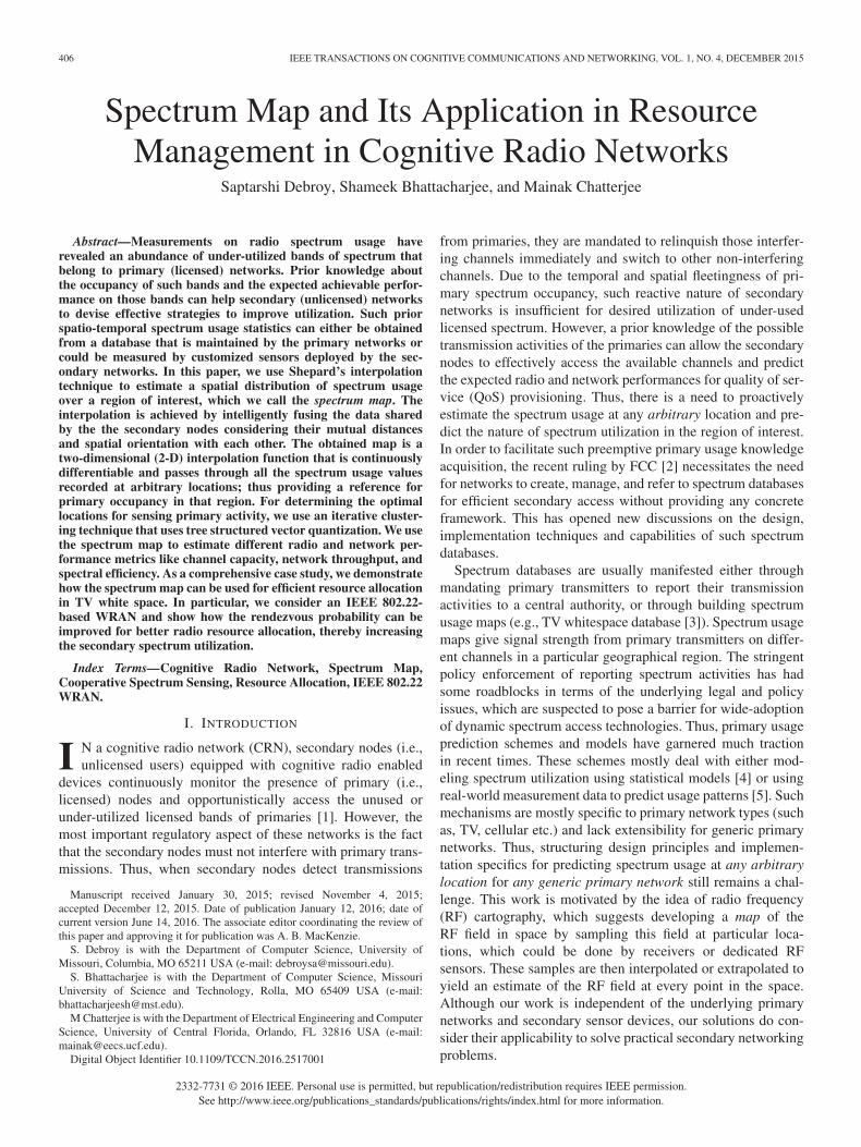
Fig. 1. Different orientations of data points influencing estimation at (xt , yt ).

pti =

⎧⎪⎪⎨⎪⎪⎩

1

dti

i f 0 < dti ≤ r

3

27

4r

(dt

i

r− 1

)2

i fr

3< dt

i ≤ r

The above function is defined to be continuously differen-tiable for all dt

i > 0. It can easily be argued that more datapoints will yield a better estimation; however, they will alsoincrease the computational complexity.

Considering the effect of distance of the data points, theestimated received energy value can be modified as:

φtq =

∑δi ∈Rt

(pt

i

)2ei

q

∑δi ∈Rt

(pt

i

)2(2)

However, this interpolation function does not captive the effectof spatial orientation of the data points i.e., the relative anglethey make with each other.

D. Direction of Data Points

First, let us demonstrate the effect of direction of data pointswith the help of an example. In Fig. 1, we see two differentorientations of data points 1, 2 and 3 with respect to target clocated at (xt , yt ). In both cases, the distances of the pointsfrom (xt , yt ) are d1, d2 and d3 respectively. In the first orien-tation, all the points are on the same side of (xt , yt ) whereasin the second orientation they are on different directions withrespect to (xt , yt ). The disparate spatial orientations in thesetwo cases yield different effects on (xt , yt ). Thus, we considerall the possible set of angles that each data point makes with allother data points.

The directional weighting term for each selected data pointδi near (xt , yt ) is given as

ati =

∑δ j ∈Rt

(pt

j

)[1 − cos � δi t δ j ]

∑δ j ∈Rt

(pt

j

) ∀ j �= i (3)

Equation (3) signifies when two sensors are on the same line,the algorithm only considers the contribution from the closersensor. When the sensors are at right angles, the algorithmweights each of them equally, and for angles in between, theweighting follows a cosine.

Now, considering the effect of number, distances, and direc-tions of data points on (xt , yt ), we define the weighing factoras wt

i = (pti )

2(1 + ati ). It is to be noted that in the directional

Algorithm 1. Interpolation algorithm

Data: Set of sensors/data points Si = {δi }Data: Target point (xt , yt )Data: Sensor radius rData: Power spectral density ei

q of data point i on channel qResult: Estimated power spectral density in a region for each

channelfor all channels q do

for all data points i in the set Si doif 0 ≤ dt

i ≤ r3 then

dis Fact ti ⇐ 1

dti

else if r3 < dt

i ≤ r then

dis Fact ti ⇐ 27

r (dt

ir − 1)2

for all data points k ∀ k �= i doangFact t

i ⇐ angFact ti + dis Fact t

i × ((xt − xi )

(xt − xk) + (yt − yi )(yt − yk))/dis Fact ti

endf nlWghtt

i ⇐ (dis Fact ti )

2(1 + angFact ti )

powSpecDnst tq ⇐ powSpecDnst t

q + f nlWghtti ×ei

q

f nlWghtti

endend

weighing term ati , the distance weighting factor pt

j is includedin the numerator and the denominator because points near(xt , yt ) should be more important in shadowing than distantpoints [25]. Thus, the final interpolated received energy forchannel chq considering the distance and direction factors is:

φtq =

∑δi ∈Rt

wti ei

q

∑δi ∈Rt

wti

(4)

Note, this is the estimated channel usage of a particularchannel chq . To get the values for the entire spectrum range,we simply repeat the computations for all the channels (letthere be N channels in the spectrum) concerned. Therefore theestimated spectrum usage at (xt , yt ) is given as:

�t = [φt

1, φt2, · · · , φt

N

](5)

The process of computing �t is shown in Algorithm 1. Theinterpolation technique meets all the requirements (i.e., definedat every point and is continuously differentiable) for computingthe spectrum usage scenario at the target location (xt , yt ). Withthe usage for the entire spectrum known, we can find the set offree channels at (xt , yt ) for which we need to apply hypothesisanalysis on every channel.

The complexity of Algorithm 1 is O(m2 N ) where N is thenumber of channels and m is the number of data points (mon-itoring secondary nodes) involved in the interpolation. Sincethe number of monitoring secondary nodes is a constant, theaverage case complexity is O(N ).

Our choice for using Shepard’s method for constructingthe spectrum map over other multi-dimensional interpolationfunctions are because of the following reasons:


Fig. 2. Estimated power spectral density with 40 sensing locations.

Fig. 3. Estimated power spectral density with 80 sensing locations.

1) Shepard’s method is inherently suited for multi-dimensional spatial data.

2) It involves simple mathematical operations with lowcomputational complexity.

3) Only a few data points are to be considered in R2.4) Time independence obviates effects of fading which

can be countered with suitable sensing and collectionfrequency.

For building the spectrum map, we do not consider sensorsreporting imprecise readings located behind obstacles. Suchphenomenon can be corrected by using other known sensorlocalization techniques where the distance d to a sensor is cor-rected as d ′ [26]. Such discussions are beyond the scope of thispaper.

E. Spectrum Map Construction From Real Data

Now we demonstrate the spatial distribution of spectrumusage and measure the accuracy of estimation. We create a gridof 100×100 units and emulate primary behavior using real-world spectrum data archive of RWTH Mobnets used in [6].The experiment performed considers 1000 channels of band-width 100 kHz each in the 2.4 GHz ISM band in Germany. Thereceived power at any receiver from primary nodes was variedfrom −45 dBm to −80 dBm.

Figures 2 and 3, show the power spectral density of primarychannel usage for one of the 1000 channels using 40 and 80data points respectively. Locations of the data points used for

interpolation are shown in darker shades. Expectedly, the sur-face plots become increasingly accurate as the number of datapoints increases. Similar results are observed for all the chan-nels. Although it seems beneficial to use as many data pointsas possible to get more accurate spectrum map, there is a trade-off between the accuracy of estimation and complexity of suchestimation. Such trade-off is dependent on other physical andenvironmental factors such as type of primary network (thresh-old signal strength to operate, probability of primary activity),accuracy of sensors involved in detecting signals, location ofthe sensors, physical environment in terms of terrain affect-ing fading and shadowing. Moreover, this trade-off is not onlydependent on the number of sensors but also on the frequencyof periodic sensing, making such trade-off modeling non-trivialand to our opinion, beyond the scope of the paper. However,we make an attempt to perform an experimental trade-off quan-tification in Section IV for a specific approach on data pointplacement.

It is to be noted that spectrum usage reports from sensorslocated in heavily faded regions will not be very effective - evenmore so when there are few sensors. We argue that, there willbe enough sensors to average out any bad readings. Moreover,the deployment of the sensors are not ad hoc. Rather, inour proposed method, their locations are determined consid-ering topological effects and primary locations which will bediscussed in Section IV.

Once the estimates of channel usage for all the channels areknown, we apply the energy detection hypothesis to decidethe channel occupancy from the interpolated values (detectedenergy) and find the set of free channels at (xt , yt ). Althoughthe proposed interpolation scheme successfully estimates thereceived signal strength of a region of interest, there are cer-tain assumptions and limitations in terms of the techniques’applicability. The are:

• The proposed model does not include channel variablesfor phenomena such as shadowing or fading to keep thealgorithmic complexity low and lightweight to make iteasily implementable on low-cost and power-constraintsensor devices.

• The proposed model works best in a slow fading and lowshadowing environment. For fast fading and shadowingenvironment, the estimation accuracy decreases; however,the estimation is always conservative. Thus the estima-tion does not generate false negative in terms of channeloccupancy.

• Since the transmitter and receiver heights are very smallcompared to the distances in the planar 2-dimensionalregion, we can project an actual 3-dimensional spectrummap on to a 2-dimensional map with minimal effect.

IV. SELECTION OF IDEAL SENSING LOCATIONS

We argue that the accuracy of the Shepard’s interpolationtechnique can be improved by selecting the data points at strate-gic locations. Be it centralized or distributed, either with a cen-tral repository or multiple fusion centers, strategically placingthe sensing locations that depend on the primary locations havea profound effect on the construction of the Spectrum Map.


Fig. 4. Iterative clustering and corresponding representation points.

Thus, we propose an iterative clustering technique using treestructured vector quantization (TSVQ) to find these representa-tion points, i.e., sensing locations. Vector quantization (VQ) isa powerful data compression technique where an ordered setof real numbers is quantized. The idea of such quantization isto find |�| representation points (distinct vectors) from a largeset of vectors so that the average distortion is minimized. Withiterative clustering, the size of the representation points growsfrom 1 to the desired value, |�|. Given a set of primary trans-mitter locations, their centroid is the ideal representation pointwhen |�| = 1, as the sum of the Euclidean distances to all theprimary transmitters is minimum at the centroid. We show anillustrated example in Fig. 4(a) where S1 denotes the centroidof the primary transmitters represented as hollow dots creatinga single cluster C1.

A. Iterative Clustering

With further iterations, S1 is split into two points, S1 andS1 + ε, where ε is a small Euclidean distance. Each of theprimary locations is grouped on to the closer of the tworepresentation points thereby creating two clusters with tworepresentation points. The centroids of these two clusters aredetermined and the representation points, S1 and S1 + ε, areupdated with the centroids’ position creating new representa-tion points S1 and S2. Clustering is performed again on thesetwo representation points till the desired size of |�| is achieved.Fig 4(b) shows the scenario with two such points correspond-ing to the two clusters C1 and C2. Further splitting into four anditeratively applying the clustering algorithm, we obtain the fourcentroids along with the four clusters as shown in Fig. 4(c). Itis to be noted that such binary splitting yields 2n clusters.

B. Choice of Number of Representation Points (|�|)The requirement of |�| in the given scenario differs from the

choice of |�| in conventional VQ. In conventional VQ, the maingoal of designing a quantizer is to find the representation pointsand the cluster such that the average distortion is minimized fora fixed number of such points. However, in a cognitive radionetwork, the choice of |�| is governed by variables like thetype of secondary network, number of primary transmitters and

density of secondary nodes. More data points obviously resultmore accurate spectrum but with more sharing and complexityoverhead. In next section, we shed more light on the accuracyof estimation with choice of |�|.

C. Performance Gains Using Iterative Clustering

We conduct simulation experiments to demonstrate the ben-efits of using iterative clustering technique over deterministicand random selection of data points. The simulation is con-ducted using C and the figures are generated using MATLAB.A fixed number of primary users (70 in this case) are deployedrandomly over a 100×100 area region. A certain number of pri-maries are chosen randomly to be active and assigned powersranging from high to low based on various primary network’stransmission patterns using RWTH Mobnets data [11].

In the first set of experiments, we compare the actual RSSvalues (calculated using a highly sophisticated and widely usedpath-loss model proposed in [27]) with the estimated values(calculated using our interpolation scheme). We choose the datapoints (representation points) according to iterative clusteringand vary the number of data points from 20 to 60. We then omit3 data points from the group of data points and reconstruct themap using our proposed interpolation scheme. The results ofactual and estimated RSS at the missing data point locationsare presented in Table I. The same experiment is run 3 differenttimes with different numbers of data points used each time toconstruct the map. We observe that in terms of dBm, the erroris negligible and with more data points the accuracy increases.

In the next set of results, we use the number of mismatchesas the metric to evaluate the benefits of using iterative cluster-ing for data point location selection. A mismatch is defined foreach channel where the the actual and the estimated binary vec-tors do not match. Fig. 5 depicts the effectiveness of iterativeclustering in estimating the spectrum map for varied primaryactivity, i.e., the probability of primary being active on a par-ticular channel. This probability is calculated by the number ofchannels where primaries are active over the total number ofchannels (100 in this case). First, we find the actual RSS in thesecondary locations for all the channels and compare the valueswith a threshold to find actual binary decision vectors. Then, weuse iterative clustering technique to find the suitable data point


TABLE ICOMPARISON BETWEEN ACTUAL AND ESTIMATED POWER SPECTRAL DENSITY (DBM/100 KHZ) AT MISSING DATA POINTS FOR

DIFFERENT NUMBER OF DATA POINTS

Fig. 5. Performance of iterative clustering for different primary activities.

Fig. 6. Comparison of different data point selection strategies.

locations for Shepard’s interpolation. From the estimated RSS,we find the estimated binary decision vectors using the samethreshold. We observe that even with high primary activity, theiterative clustering performs fairly well in terms of mismatcheswhen there are more than 16 data points selected for interpola-tion. For low primary activity, the average mismatch is less than10% for any number of selected data points.

In Fig. 6, we compare the performance of the proposediterative clustering technique with random and deterministicselection of data points. In deterministic selection, data pointsare chosen uniformly in a grid-like orientation to cover theentire region without considering the locations of the primaries.The performance comparison is made for low primary activityof value 0.3. From the figure, we observe that even for low pri-mary activity, iterative clustering performs better than randomand deterministic selections in terms of average mismatches forany number of selected data points for interpolation. We alsoobserve that, especially for random selection the number of

mismatches vary more than iterative and deterministic scenar-ios proving random selection being the most imprudent choice.We also observe that accuracy of estimation is not only a func-tion of location of data points selected, but also on the numberof data points and primacy activity. This makes the theoreticalquantification of trade-offs between accuracy and complexityof estimation is non-trivial and in our opinion, an independentavenue of research altogether.

V. PREDICTING CHANNEL PERFORMANCE METRICS

We extend our spectrum usage prediction model to predictthe performance of a secondary transmitter-receiver pair andalso the secondary network as a whole. We assume a scenariowhere K secondary nodes are exposed to M primary users. Asecondary receiver is interfered by potentially all transmitterson all possible channels.

The interference experienced by a secondary receiver at(xt , yt ) is due to the primary transmitters as well as otherreceivers using the same channel. Let us suppose that theinterference experienced receiver at (xt , yt ) from all primarytransmitters is ϕt

q .

The received signal power at (xt , yt ) is given by P|htq |2,

where P is the transmit power of the corresponding secondarytransmitter and ht

q is the channel gain between the secondarytransmitter-receiver pair. The channel gain between the two sep-arated by a distance Dt is given by ht

q = ADα/2

t; where A is a

frequency dependent constant and α is the path loss exponent.Let I t

q is the interference the receiver at (xt , yt ) experiencesfrom another secondary communication in the cell using samechannel chq . Then

I tq =

∑∀ j∈κq

P∣∣∣h j

q

∣∣∣2(6)

where κq is the set of all other secondary pairs usingchannel chq .

With the above parameters defined, we show how the we cancalculate critical channel performance metrics, such as, channelcapacity, spectral efficiency, and secondary throughput. Witheach performance metric we provide simulation results of thecorresponding metric using the same experimental environmentdescribed in Section III-E.

A. Channel Capacity

We use Shannon-Hartley’s capacity model for a band-limitedchannel with additive white Gaussian noise (AWGN) [28].Thus, we express the channel capacity Ct

q for channel chq as


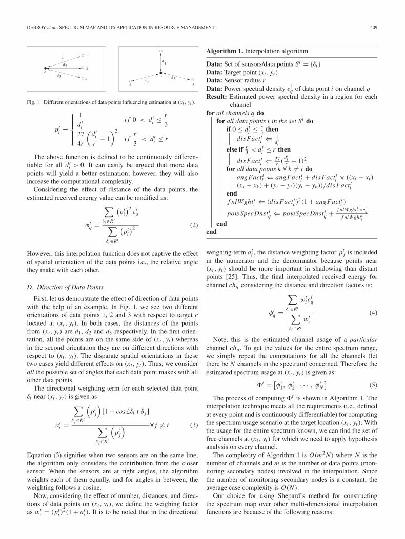
Fig. 7. Channel capacity characteristics.

Ctq = B log2

⎛⎜⎝1 +

P∣∣∣ht

q

∣∣∣2

ϕtq + I t

q

⎞⎟⎠ (7)

where B is the channel bandwidth. Note that the channel capac-ity is dependent on the channel used by the transmitter-receiverpair as the interference experienced from primary transmittersand other secondary communication are different on differentchannels.

In Fig. 7(a), we show the channel capacity characteristicsfor an arbitrary receiver location calculated using Equation (9).The figure shows different channel capacity values for 1000channels of 100KHz each in the 2.4 GHz ISM band. Suchrepresentation of channel capacity can be exploited by a par-ticular transmitter-receiver pair for selecting better channels interms of achievable capacity when multiple such free channelsare available for communication. Through another 3D repre-sentation shown in Fig. 7(b), we present the channel capacityvalues (calculated using Eqn. (7)) of a particular channel andfor a particular transmitter and multiple potential receiverlocations. Such representation can be further exploited for:a) optimal allocation of a particular channel to the best con-tending secondaries, and b) optimal location selection of asecondary node (in cases where secondary node installation ispre-planned) for statistically empty channels. Both approachesshown in figures 7(a) and 7(b) are highly effective for bettersecondary utilization. Later in Section VI-E we will show howthis expected channel capacity information can be utilized forefficient channel allocation in an IEEE 802.22 network.

B. Secondary Network Throughput

Secondary network throughput depends on the number ofsecondary pairs in a network using the same channel. If thesecondary transmitter transmits with power P to receiver at(xt , yt ), then the transmission rate considering all other sec-ondary communication is given by

π tq = log

⎛⎜⎝1 +

P∣∣∣ht

q

∣∣∣2

I tq + ϕt

q + σ 2

⎞⎟⎠ (8)

where the received signals are corrupted by zero-mean additivewhite Gaussian noise of power σ 2.

To obtain the network throughput for the channel chq , wesum the transmission rates of all the secondary pairs using chq

as [29]:

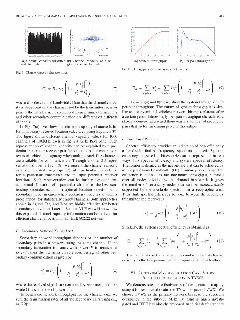
Fig. 8. Throughput estimation using spectrum map.

�q =∑

∀ j∈κq

π tq =

∑∀ j∈κq

log

⎛⎜⎝1 +

P∣∣∣ht

q

∣∣∣2

I tq + ϕt

q + σ 2

⎞⎟⎠ (9)

In figures 8(a) and 8(b), we show the system throughput andper-pair throughput. The nature of system throughput is sim-ilar to a conventional wireless network hitting a plateau aftera certain point. Interestingly, per-pair throughput characteristicshows a convex nature and there exists a number of secondarypairs that yields maximum per-pair throughput.

C. Spectral Efficiency

Spectral efficiency provides an indication of how efficientlya bandwidth-limited frequency spectrum is used. Spectralefficiency measured in bits/sec/Hz can be represented in twoways: link spectral efficiency and system spectral efficiency.The former is defined as the net bit-rate that can be achieved bya link per channel bandwidth (Hz). Similarly, system spectralefficiency is defined as the maximum throughput, summedover all nodes, divided by the channel bandwidth. It givesthe number of secondary nodes that can be simultaneouslysupported by the available spectrum in a geographic area.Thus, link spectral efficiency for chq between the secondarytransmitter and receiver is

ξ tq = 1

Blog

⎛⎜⎝1 +

P∣∣∣ht

q

∣∣∣2

I tq + ϕt

q+ σ 2

⎞⎟⎠ (10)

Similarly, the system spectral efficiency is obtained as

�q =∑

∀ j∈κq

ξ tq = 1

B

∑∀ j∈κq

log

⎛⎜⎝1 +

P∣∣∣ht

q

∣∣∣2

I tq + ϕt

q+ σ 2

⎞⎟⎠ (11)

The nature of spectral efficiency is similar to that of channelcapacity as the two parameters are proportional to each other.

VI. SPECTRUM MAP APPLICATION CASE STUDY:RESOURCE ALLOCATION IN TVWS

We demonstrate the effectiveness of the spectrum map byusing it for resource allocation in TV white space (TVWS). Wechoose TVWS as the primary network because the spectrumoccupancy in the sub-900 MHz TV band is much investi-gated and IEEE has already proposed an initial draft standard


Fig. 9. Architecture of an IEEE 802.22 network.

(IEEE 802.22 WRAN) [7] to exploit these unused bands. Thecore components of an IEEE 802.22 WRAN are base sta-tions (BS) and consumer premise equipments (CPE) as shownin Fig. 9. Secondary nodes (BSs and CPEs) opportunisticallyaccess unused or underutilized TV bands when not in use.

A. Network Model

1) Primary Network: The primary network consists of TVtransmitters, TV receivers and wireless microphones with thelatter taking only a small amount of band space. The TV trans-mitters are deployed depending on population density in ageographic region. An urban area has denser transmitters thanrural regions. In Section VI-E3, we try to emulate the locationdistribution of TV transmitters from existing literature surveys.We assume that the signal diffuses isotropically in the environ-ment and is then received by xi with intensity P multiplied by aloss factor of l(xi ,x j ) due to isotropic dispersion and absorptionin the environment.

2) Secondary Network: IEEE 802.22 networks are central-ized CRNs divided into cells, each having one BS. The BScommunicates with the CPEs in its cell as well as with neigh-boring BSs. The BS is aware of the location of all the CPEsunder it. We assume that there are no pre-defined control chan-nels in the system, i.e., the only means of communicationbetween the BS and the CPEs are the free channels that arecurrently not being used by the primary users. Each BS has twoprocessing units responsible for two sets of functions. Periodicspectrum sensing, sharing the sensed spectrum data and creat-ing the spectrum map is performed by one unit and the other isresponsible for beacon broadcast to advertise free channels andQoS provisioned allocation of the free channels to the CPEs.The latter functions are performed after consulting the latestversion of spectrum map. Details of the allocation process isdiscussed in Section VI-E2.

CPEs are also equipped with sensing devices for findingunused channels; however, performing spectrum sensing isintelligent and selective depending on the state of the node dis-cussed in Section VI-E1. CPEs are allocated a pair of uplink anddownlink channels which they are allowed to use till a primaryarrives or unless they relinquish the channels themselves.

B. Resource Allocation Problem

The main challenge in allocating channels to the CPEs is theabsence of pre-defined control channels between the BS and the

CPEs. Upon detection of any transmission activity from a pri-mary user on a channel, the secondary nodes are mandated torelinquish those channels [30]. The ability of the BS to assignthe best possible channels to the CPEs depends on how wellthe BS is able to capture the spectrum availability at the variousCPE locations. Since the BS cannot perform sensing at loca-tions other than itself, it has to rely upon the sensed spectrumreports shared by the CPEs. If all the CPEs were to continu-ously share their spectrum usage reports, the BS would have themost accurate information. However, the communication over-head becomes a bottleneck as sharing of data has to be doneon the same channels that the BS is supposed to allocate. Thus,channel assignment to CPEs becomes a challenge.

C. Our Solution Using the Spectrum Map

We design an on-demand channel allocation scheme forIEEE 802.22 networks using our proposed spectrum map. Welet a subset of CPEs to work as data points and feed theirspectrum usage data to the BS for it to create the spectrummap. The spectrum map allows a two-fold solution for efficientresource allocation. First, the map is used for quicker commu-nication with a candidate CPE and increases the probabilityof rendezvous between the CPE and the BS. Such commu-nication allows the BS to acquire the actual spectrum usageat the CPE and evaluate different performance metrics. Suchproactive performance analysis not only identifies the best can-didate channel for a CPE but also indicates the best possibleCPE among candidate CPEs for a particular channel. Channelallocation scheme thus adopted increases the overall networkthroughput and maximizes spectrum usage.

D. Improving Rendezvous Probability Using Spectrum Map

The means of initial communication between the BS and aCPE looking for channels is the beacons sent by the BS andsubsequent handshaking process. The latest IEEE 802.22 basedWRAN specifications [8] mandate the MAC layer to be able toadapt dynamically to changes in the environment by sensingthe spectrum. Although the MAC layer is mandated to con-sist of specific data structures, details about the mechanismand involved channels (i.e., dedicated common control chan-nel or dynamic channel rendezvous) for such rendezvous arenot specified. However, in the absence of any control channel,this communication is probabilistic, i.e., the BS can send bea-cons with the specific data structures on the available channelsand hope that the CPEs respond. Although viable, this tradi-tional technique is ineffective and probability of rendezvousbetween the BS and a CPE is low. We propose an intelligentbeacon broadcast scheme with the help of the spectrum mapthat can minimize the number of channels where beacons aresent and thus increasing the probability of dynamic rendezvouswith the CPEs. This obviates the need for a any control channelbetween the BS and the CPEs making the secondary com-munication completely opportunistic. In the intelligent beaconbroadcasting scheme, the beacons are sent only on selectedchannels depending on the requirement of idle CPEs. Theseselected channels are those that belong to the common set of


the available channels at the BS and the set of channels whichare estimated to be available for the idle CPEs (from spectrummap). The BS sends beacons in each of this common pool ofchannels and waits for channel allocation request from any nodeand after a stipulated time moves to the next channel. In case ofsuccessful reception of a channel allocation request, the BS logsthe request before moving to next channel. At the end of thebeacon cycle, the BS proceeds to allocate channels to the nodeswhose channel allocation requests were successfully receivedduring the beacon broadcast cycle. Such prediction of channelusage at CPE and sending beacons only on the potential freechannels reduce interference to primaries.

Let us assume that there are K CPEs in a cell tuning period-ically to N channels in order to receive a BS beacon. Thereforeinitially,

Prob{A CPE receiving a beacon} = 1

N

Let us also assume that out of K CPEs, |�| have been alreadybeen delegated for sensing. From the remaining K − |�| CPEs,let the probability that a CPE is allocated at any instance bepalloc. Therefore, if |J | is the set of idle CPEs in the system atany time then,

|J | = K − (K − |�|) × palloc − |�|We also assume that γ b

f ree and γ if ree are the sets of free chan-

nels at the BS and at any CPE i as estimated by the BS usingthe spectrum map (|γ b

f ree|, |γ if ree| ≤ N ). Now from γ i

f ree∀i ,the BS can estimate the entire set of free channels for the cellas γ cell

f ree = ⋃i∈J γ i

f ree and use the channels belonging to the

set γ bf ree

⋂γ cell

f ree only; thus initiating the intelligent beaconbroadcast scheme.

Now for a successful handshake between a BS and aCPE, ideally only a single CPE should reply to the beaconwith a channel allocation request. More than one reply willcause interference resulting in unsuccessful reception. Thus,collision is only possible when more than one CPE listen to abeacon on the same channel at the same time. Therefore, theprobability of a successful rendezvous in a beacon period, Pren

is expressed as:

Pren = Prob {Beacon is sent on a channel and only a single

CPE is tuned to the channel}= Prob {A single CPE tuned to a channel | beacon was

sent on that channel}Since the tuning by a CPE and the beacon broadcast aremutually independent,

Pren = Prob{A single CPE is tuned to a channel}

= |J | × 1

N×

(1 − 1

N

)|J |(12)

Therefore, the expected number of successful handshakes perbeacon period is,

E[No. of successful handshakes] =∣∣∣γ b

f ree

⋂γ cell

f ree

∣∣∣ × Pren

Fig. 10. Benefits of proposed beacon broadcast technique in terms of beaconreception.

Fig. 11. Nature of probability of a successful handshake.

It is to be noted that the above analysis considers an aggres-sive transmission-reception strategy adopted by the CPEs, i.e.,the CPEs do not wait before transmitting the channel allocationrequest. In the other alternative, i.e., the non-persistent strategywhere CPEs wait for a time window before sending channelallocation request, the possibility of collision between CPEsdecreases. Therefore, the above analysis considers the worstcase performance in terms of probability of a successfulrendezvous.

1) Numerical Results: To better elucidate the advantages ofproposed intelligent beacon broadcast over conventional proba-bilistic technique, we perform numerical analysis in MATLABcapturing the spatial correlation among nodes, and interferenceamong CPEs. The probability of a channel being free is kept at0.3.

In Fig. 10, we compare the probabilities of a CPE receiv-ing a beacon for conventional and proposed intelligent beaconbroadcast schemes. We see that irrespective of the total numberof channels in the spectrum, the probability is higher with theintelligent beacon broadcasting technique.

In Fig. 11, we observe the nature of Pren from Eqn. (12).There exists a convexity where the probability of handshakeincreases with number of unallocated CPEs and graduallydecreases afterwards. The gradual decrease is due to the lim-ited channel availability for increasing unallocated CPEs. Withmore channels in the system, the saturation point is with higher


Fig. 12. Benefits of proposed beacon broadcast technique in terms of expectednumber of successful handshakes.

value of unallocated CPEs. However, the maximum numberof CPEs allowed in a cell is 255 [8] and the number ofsimultaneous unallocated CPEs will be even less.

Fig. 12 compares the performance of the proposed intelligentbeacon broadcast with conventional probabilistic rendezvoustechnique in terms of expected number of successful hand-shakes in a beacon period. We observe that with any numberof unallocated CPEs, the proposed technique performs betterthan conventional beacon broadcast.

E. Channel Allocation

In order to efficiently allocate channels to the CPEs, weuse iterative clustering as was discussed in Section IV to finddelegation among the CPEs to work as data points.

1) Delegation CPEs With Iterative Clustering: We createzones are logical divisions of the coverage area of a BS. Thezones are equivalent to the clusters discussed in Section IV.This division is proposed as a BS specific feature and there-fore does not violate the specifications [30]. Each of such zones(clusters) has a cluster-head which is the designated data pointfor that zone. We call these data-points as Delegation CPEs.BS controls the selection of a particular CPE as a delegationmember. The idea is to have almost equal representation fromall zones and no zone is unrepresented as far as possible. TheBS maintains three queues for each zone, namely: AQ (for allo-cated CPEs), DQ (for delegated CPEs) and HQ (for potentiallydelegate CPEs i.e., idle CPEs with channels). Selection of adelegation member takes place after termination of data trans-mission (either voluntarily or forcefully) with the channel usednow serving as sharing medium. If not selected for delegation,a CPE can relinquish its channels or hold onto the channels inanticipation of channel requirement in the near future. Holdingtime depends on the demand for the particular channels by otherCPEs. However, such holding onto channels can result in thatCPE being selected as a delegation member (using the samechannels for sharing) if instructed by the BS. A delegated CPEcontinues to serve until it is instructed otherwise by the BS. Thisobligates the CPE to use the allocated channels only as meansto share its spectrum usage with BS even if the CPE wants to goto the transmission state. The decision of keeping such a CPE

Fig. 13. IEEE 802.22 network with BS and different types of CPEs.

in sharing state solely depends on the importance of that CPE inbuilding the spectrum profile. Soon after the BS finds a suitablealternative, it allows the CPE to switch to the transmission stateand use the same channel for data communication.

Fig. 13 is an illustrative example that shows how the coveragearea of the BS is divided into zones. The BS attempts to find adelegated CPE for every zone.

2) Allocation Process: The allocation process by the BS isinitiated by reception of a channel allocation reply from anyCPE c on any of the νest ∩ γ b

f ree ∩ γ cf ree channels. Such allo-

cation reply is accompanied with raw spectrum usage at c,ϒc={φc

j |∀ch j ∈ N }. The BS creates the set of available chan-nels ρc

avl={ j |∀φcj < T } allocable to c. Channels used by other

allocated or delegated CPEs in the interference range of c cannot be allocated to c for obvious reasons. In order to ensure this,the BS maintains the AQ, DQ and HQ of all the zones withinthe interference range of c. From the AQs, the BS creates theset AQ

cwith only those channels which are allocated to CPEs

within the interference range of c. Similarly DQc

and H Qc

arecreated. No channels in AQ

cand DQ

ccan be allocated to avoid

co-channel interference. BS updates the set of available chan-nels for allocation ρc

avl excluding all such channels. For all therest of the channels in ρc

avl , expected channel performance (canbe any desirable parameter or a combination of some) is calcu-lated and given a score. ρc

avl is further updated with descendingorder of the channel scores. There is also the set H Q

cwhose

channels are held by other idle CPEs in the interference range ofc. The purpose for allowing the CPEs to hold onto channels isto expedite channel allocation by not making them go throughthe entire handshaking process. Therefore, BS always tries toallocate the best channel among |ρc

avl | not belonging to H Qc,

if possible.3) Experimental Results: In a completely new experimen-

tal set-up to the one discussed in Section III-E, we simulatethe locations of TV stations in a 500 × 500 sq. miles grid asshown in Fig 15 using TV station location distribution in [4].The total number of channels is varied from 50-400 with corre-sponding bandwidth of 6 MHz-750 kHz. The power-profile ofthe TV stations ranges between 10kW-1MW. We identify tworegions with dense and sparse primary densities (mimickingbig cities and small towns) and deploy IEEE 802.22 networks(WRAN cells) shown in Fig. 15. Locations of different typesof nodes and transmission patterns are different in the two sce-narios while total number of CPEs, density, and the number ofdelegated CPEs are kept the same.


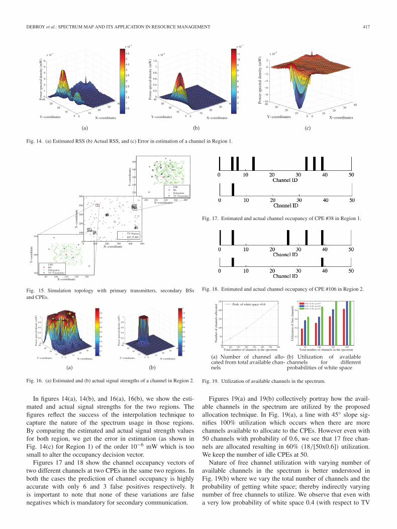
Fig. 14. (a) Estimated RSS (b) Actual RSS, and (c) Error in estimation of a channel in Region 1.

Fig. 15. Simulation topology with primary transmitters, secondary BSsand CPEs.

Fig. 16. (a) Estimated and (b) actual signal strengths of a channel in Region 2.

In figures 14(a), 14(b), and 16(a), 16(b), we show the esti-mated and actual signal strengths for the two regions. Thefigures reflect the success of the interpolation technique tocapture the nature of the spectrum usage in those regions.By comparing the estimated and actual signal strength valuesfor both region, we get the error in estimation (as shown inFig. 14(c) for Region 1) of the order 10−6 mW which is toosmall to alter the occupancy decision vector.

Figures 17 and 18 show the channel occupancy vectors oftwo different channels at two CPEs in the same two regions. Inboth the cases the prediction of channel occupancy is highlyaccurate with only 6 and 3 false positives respectively. Itis important to note that none of these variations are falsenegatives which is mandatory for secondary communication.

Fig. 17. Estimated and actual channel occupancy of CPE #38 in Region 1.

Fig. 18. Estimated and actual channel occupancy of CPE #106 in Region 2.

Fig. 19. Utilization of available channels in the spectrum.

Figures 19(a) and 19(b) collectively portray how the avail-able channels in the spectrum are utilized by the proposedallocation technique. In Fig. 19(a), a line with 45◦ slope sig-nifies 100% utilization which occurs when there are morechannels available to allocate to the CPEs. However even with50 channels with probability of 0.6, we see that 17 free chan-nels are allocated resulting in 60% (18/[50x0.6]) utilization.We keep the number of idle CPEs at 50.

Nature of free channel utilization with varying number ofavailable channels in the spectrum is better understood inFig. 19(b) where we vary the total number of channels and theprobability of getting white space; thereby indirectly varyingnumber of free channels to utilize. We observe that even witha very low probability of white space 0.4 (with respect to TV


Fig. 20. Number of allocated CPEs for different number of channels.

Fig. 21. Normalized supported data rate for different number of idle CPEs.

spectrum), the proposed allocation scheme ensures more than50% utilization of free spectrum in most occasions. The totalnumber of allocable CPEs are kept at 255 for all the scenariosabove which is the maximum number of CPEs that an IEEE802.22 cell can have [30].

In Fig. 20, we show the efficiency of the proposed allocationtechnique by calculating the number of CPEs being allocateda pair of uplink and downlink channels. We observe that with400 channels and a probability of getting white space of 0.8, weallocate 106 out of possible 160 CPEs.

In Fig. 21, we compare the performances of channel alloca-tion with and without using spectrum map for different numberof free channels in terms of normalized supported data rate.We define normalized aggregate data rate as the aggregate bitrate supported by the allocated channels to the total achiev-able capacity of the free channels. We see that except the casewith 50 free channels, the spectrum map initiated allocationperforms better. For very low number of available channels,if there are more idle CPEs, it creates more collision duringbeacon broadcast phase resulting less utilization.

VII. CONCLUSION

In this paper, we use Shepard’s interpolation technique tocreate a spectrum map, i.e., an estimate of the spectrum usageat any arbitrary location in a secondary cognitive radio network.

This is achieved by sharing and fusing raw spectrum datasensed at various strategic locations computed using itera-tive clustering. We demonstrate how the spectrum map canhelp in predicting channel performance metrics, such as, chan-nel capacity, spectral efficiency, and secondary throughput.Through simulation experiments, we validate the correctness ofthe map and show how we can compute the distribution of thesemetrics at any arbitrary location, which can potentially be usedby secondary networks for better channel selection to maximizespectrum usage. Finally, we demonstrate how the proposed maphelps attain near perfect channel allocation in IEEE 802.22networks and improve channel rendezvous probability.

REFERENCES

[1] I. F. Akyildiz, W.-Y. Lee, M. C. Vuran, and S. Mohanty, “Next generation/dynamic spectrum access/cognitive radio wireless networks: A survey,”Comput. Netw. J., vol. 50, pp. 2127–2159, 2006.

[2] FCC Adopts Rule for Unlicensed Use of Television White Spaces[Online]. Available: https://www.fcc.gov/document/tv-white-spaces-rule-changes/

[3] Google Spectrum Database [Online]. Available: https://www.google.com/get/spectrumdatabase/

[4] J. Riihijarvi and P. Mahonen, “Exploiting spatial statistics of primary andsecondary users towards improved cognitive radio networks,” in Proc. 3rdInt. Conf. Cognit. Radio Oriented Wireless Netw. Commun. (CrownCom),May 2008, pp. 1–7.

[5] Y. Li, T. T. Quang, Y. Kawahara, T. Asami, and M. Kusunoki, “Buildinga spectrum map for future cognitive radio technology,” in Proc. ACMWorkshop Cognit. Radio Netw. (CoRoNet’09), 2009, pp. 1–6.

[6] J. Riihijarvi, P. Mahonen, M. Wellens, and M. Gordziel, “Characterizationand modeling of spectrum for dynamic spectrum access with spatialstatistics and random fields,” in Proc. IEEE 19th Int. Symp. Pers. IndoorMobile Radio Commun. (PIMRC), Sep. 2008, pp. 1–6.

[7] IEEE 802.22, Working Group on Wireless Regional Area Networks(WRAN) [Online]. Available: http://grouper.ieee.org/ groups /802/22

[8] IEEE Draft Standard for Wireless Regional Area Networks—Part 22:Cognitive Wireless Ran Medium Access Control (MAC) and PhysicalLayer (PHY) Specifications: Policies and Procedures for Operation inthe TV Bands—Amendment: Management and Control Plane Interfacesand Procedures and Enhancement to the Management Information Base(MIB), IEEE P802.22a/D2, Oct. 2013, pp. 1–551.

[9] M. A. McHenry, D. McCloskey, D. Roberson, and J. T. MacDonald,“Spectrum occupancy measurements—Chicago, Illinois,” SharedSpectrum Company, Tech. Rep., 2005.

[10] T. Harrold, R. Cepeda, and M. Beach, “Long-term measurements of spec-trum occupancy characteristics,” in Proc. IEEE Int. Symp. New Front.Dyn. Spectr. Access Netw. (DySPAN), May 2011, pp. 83–89.

[11] V. Atanasovski et al., “Constructing radio environment maps with het-erogeneous spectrum sensors,” in Proc. IEEE Int. Symp. New Front. Dyn.Spectr. Access Netw. (DySPAN), May 2011, pp. 660–661.

[12] B. Jayawickrama, E. Dutkiewicz, I. Oppermann, G. Fang, and J. Ding,“Improved performance of spectrum cartography based on compressivesensing in cognitive radio networks,” in Proc. IEEE Int. Conf. Commun.,2013, pp. 5657–5661.

[13] A. Stirling, “Exploiting hybrid models for spectrum access: Building onthe capabilities of geolocation databases,” in Proc. IEEE Int. Symp. NewFront. Dyn. Spectr. Access Netw. (DySPAN), May 2011, pp. 47–55.

[14] R. Murty, R. Chandra, T. Moscibroda, and P. Bahl, “Senseless: Adatabase-driven white spaces network,” IEEE Trans. Mobile Comput.,vol. 11, no. 2, pp. 189–203, Feb. 2012.

[15] M. Wellens, J. Riihijarvi, and P. Mahonen, “Modeling primary systemactivity in dynamic spectrum access networks by aggregated ON/OFF-processes,” in Proc. 6th Annu. IEEE Commun. Soc. Conf. Sensor MeshAd Hoc Commun. Netw. (SECON) Workshops, Jun. 2009, pp. 1–6.

[16] M. Wellens, J. Riihijärvi, and P. Mähönen, “Full length article: Empiricaltime and frequency domain models of spectrum use,” Phys. Commun.,vol. 2, nos. 1–2, pp. 10–32, Mar. 2009.

[17] J. Bazerque, G. Mateos, and G. Giannakis, “Group-lasso on splines forspectrum cartography,” IEEE Trans. Signal Process., vol. 59, no. 10,pp. 4648–4663, Oct. 2011.


[18] H. Yilmaz, C.-B. Chae, and T. Tugcu, “Sensor placement algorithmfor radio environment map construction in cognitive radio networks,”in Proc. IEEE Wireless Commun. Netw. Conf. (WCNC), Apr. 2014,pp. 2096–2101.

[19] R. Mahapatra and E. Strinati, “Interference-aware dynamic spectrumaccess in cognitive radio network,” in Proc. IEEE 22nd Int. Symp. Pers.Indoor Mobile Radio Commun. (PIMRC), Sep. 2011, pp. 396–400.

[20] D. Denkovski, V. Atanasovski, L. Gavrilovska, J. Riihijarvi, andP. Mahonen, “Reliability of a radio environment map: Case of spa-tial interpolation techniques,” in Proc. 7th Int. ICST Conf. Cognit.Radio Oriented Wireless Netw. Commun. (CROWNCOM), Jun. 2012,pp. 248–253.

[21] J. Riihijarvi, J. Nasreddine, and P. Mahonen, “Demonstrating radio envi-ronment map construction from massive data sets,” in Proc. IEEE Int.Symp. Dyn. Spectr. Access Netw. (DYSPAN), Oct. 2012, pp. 266–267.

[22] G. Ganesan and Y. Li, “Cooperative spectrum sensing in cognitiveradio—Part I: Two user networks,” IEEE Trans. Wireless Commun.,vol. 6, no. 6, pp. 2204–2213, Jun. 2007.

[23] A. Ghasemi and E. Sousa, “Collaborative spectrum sensing for oppor-tunistic access in fading environments,” in Proc. IEEE Int. Symp. NewFront. Dyn. Spectr. Access Netw. (DySPAN), 2005, pp. 131–136.

[24] E. Visotsky, S. Kuffner, and R. Peterson, “On collaborative detectionof TV transmissions in support of dynamic spectrum sharing,” in Proc.IEEE Int. Symp. New Front. Dyn. Spectr. Access Netw. (DySPAN), 2005,pp. 338–345.

[25] D. Shepard, “A two-dimensional interpolation function for irregularly-spaced data,” in Proc. 23rd ACM Nat. Conf., 1968, pp. 517–524.

[26] M. Sen, I. Banerjee, M. Chatterjee, and T. Samanta, “Sensor localiza-tion using received signal strength measurements for obstructed wirelesssensor networks with noisy channels,” in Proc. IEEE Wireless Commun.Netw. Conf. Workshops (WCNCW), Mar. 2015, pp. 47–51.

[27] Z. Rena, G. Wanga, Q. Chena, and H. Lib, “Modelling and simulationof Rayleigh fading, path loss, and shadowing fading for wireless mobilenetworks,” Simul. Modell. Practice Theory, vol. 19, no. 2, pp. 626–637,2011.

[28] C. E. Shannon, “A mathematical theory of communication,” SIGMOBILEMobile Comput. Commun. Rev., vol. 5, no. 1, pp. 3–55, Jan. 2001.

[29] S.-W. Jeon, N. Devroye, M. Vu, S.-Y. Chung, and V. Tarokh, “Cognitivenetworks achieve throughput scaling of a homogeneous network,” IEEETrans. Inf. Theory, vol. 57, no. 8, pp. 5103–5115, Aug. 2011.

[30] IEEE P802.22/d1.0 Draft Standard for Wireless Regional AreaNetworks—Part 22: Cognitive Wireless RAN Medium Access Control(MAC) and Physical Layer (PHY) Specifications: Policies andProcedures for Operation in the TV Bands, Apr. 2008.

Saptarshi Debroy received the B.Tech. degree ininformation technology from West Bengal Universityof Technology, Kolkata, India, the M.Tech. degreein distributed and mobile computing from JadavpurUniversity, Kolkata, India, and the Ph.D. degreein computer engineering from the University ofCentral Florida, Orlando, FL, USA, in 2006,2008, and 2014, respectively. He is a PostdoctoralFellow with the Virtualization, Multimedia andNetworking (VIMAN) Laboratory, Department ofComputer Science, University of Missouri-Columbia,

Columbia, MO, USA. His research interests include cloud computing, bigdata networking, cognitive radio networks, and QoE provisioning for onlinemultiplayer gaming. He has served as Publicity Co-Chair for ACM MoViD2013, TPC member of conferences such as the IEEE GCNC, the IEEEBigDataService, ICA3PP, the IFIP/IEEE QCMan, the IEEE ANTS, the IEEEICNC, and reviewer for several international conferences and journals. He wasthe recipient of multiple awards including the IEEE PIMRC best paper award,multiple U.S. National Science Foundation (NSF), the IEEE Comsoc TravelGrant Awards, and an academic year Gold Medal at Jadavpur University.

Shameek Bhattacharjee received the B.Tech.degree in information technology from West BengalUniversity of Technology, Kolkata, India, and theM.S. and Ph.D. degrees in computer engineeringfrom the University of Central Florida, Orlando,FL, USA, in 2009, 2011, and 2015, respectively.He is currently a Postdoctoral Research Fellowwith CReWMAN Laboratory, Missouri Universityof Science and Technology, Rolla, MO, USA.His research interests include dynamic spectrumaccess networks, trust and reputation scoring and

information assurance in networking systems. He also serves as a TPC memberand reviewer of several international conferences and peer-reviewed journals.He was the recipient of the IEEE PIMRC Best Paper Award.

Mainak Chatterjee received the B.Sc. degree(Hons.) in physics from the University of Calcutta,Kolkata, India, the M.E. degree in electrical com-munication engineering from the Indian Institute ofScience, Bangalore, India, and the Ph.D. degreein computer science and engineering from theUniversity of Texas at Arlington, Arlington, TX,USA. He is an Associate Professor with theDepartment of Electrical Engineering and ComputerScience, University of Central Florida, Orlando, FL,USA. He has authored more than 150 conferences

and journal papers. His research interests include economic issues in wirelessnetworks, applied game theory, cognitive radio networks, dynamic spectrumaccess, and mobile video delivery. He co-founded the ACM Workshop onMobile Video (MoVid). He serves on the Editorial Board of the journalsComputer Communications (Elsevier) and Pervasive and Mobile Computing(Elsevier). He has served as the TPC Co-Chair of several conferences includ-ing the ICDCN 2014, the IEEE WoWMoM 2011, the WONS 2010, the IEEEMoVid 2009, Cognitive Radio Networks Track of the IEEE GLOBECOM2009, and ICCCN 2008. He also serves on the executive and technical pro-gram committee of several international conferences. He was the recipient ofthe Best Paper Awards in the IEEE GLOBECOM 2008, the IEEE PIMRC 2011,the AFOSR sponsored Young Investigator Program (YIP) Award.

spectrum map and its application in resource management in

Documents