Spectrophotometry of Very Bright Stars in the Southern Sky

Kevin Krisciunas,1,2 Nicholas B. Suntzeff,1,2 Bethany Kelarek,1 Kyle Bonar,1 and Joshua

Stenzel1

ABSTRACT

We obtained spectra of 26 bright stars in the southern sky, including Sirius,

Canopus, Betelgeuse, Rigel, Bellatrix, and Procyon, using the 1.5-m telescope at

Cerro Tololo Inter-American Observatory and its grating spectrograph RCSPEC.

A 7.5 magnitude neutral density filter was used to keep from saturating the CCD.

Our spectra are tied to a Kurucz model of Sirius with T = 9850 K, log g = 4.30,

and [Fe/H] =+0.4. Since Sirius is much less problematic than using Vega as a

fundamental calibrator, the synthetic photometry of our stars constitutes a Sirius-

based system that could be used as a new anchor for stellar and extragalactic

photometric measurements.

Subject headings: Stars - spectra

1. Introduction

Flux calibration, whether it be for photometry or spectroscopy, is a fundamental aspect

of observational astronomy (Hearnshaw 1996, 2014). Vega (α Lyr) has been a fundamental

photometric and spectroscopic standard for decades (Hayes & Latham 1975; Bohlin 2014;

Bohlin, Gordon, & Tremblay 2014). In the 1980’s the Infrared Astronomy Satellite (IRAS)

discovered circumstellar material around Vega. Subsequently, observations with the Spitzer

Space Telescope characterized this material as a debris disk (Su et al. 2005, 2013). Vega may

be spectroscopically variable as well (Butkovskaya 2014). Bohlin (2014) comments on the

non-variability of Vega. In any case Vega is problematic as a fundamental calibrator.

The Sloan Digital Sky Survey committed to using four principal photometric standards

(Fukugita et al. 1996), but in the end relied primarly on the star BD +17◦4708. Recently, it

1Texas A. & M. University, Department of Physics & Astronomy, 4242 TAMU, College Station, TX

77843; krisciunas@physics.tamu.edu

2George P. and Cynthia Woods Mitchell Institute for Fundamental Physics & Astronomy

arX

iv:1

702.

0160

2v2

[as

tro-

ph.S

R]

19

Feb

2017

– 2 –

was revealed that this star brightened by 0.04 mag in the UBV R bands from 1986 to 1991

(Bohlin & Landolt 2015).

Here we present a set of bright spectrophotometric standards, many of the brightest

stars visible in the southern hemisphere during the southern summer. Our data expand the

lists of stars observed by Hamuy et al. (1992, 1994) and Stritzinger et al. (2005). Given the

increase in sensitivity of instrumentation over the years, it might be the first time in 40 years

that carefully calibrated spectra of most of these bright stars have been obtained. Using well

defined bandpasses (Bessell 1990), we can use our spectra to generate BV RI photometry

tied to a model of Sirius, which is a “well behaved” star compared to Vega.

2. The Target Stars

The target stars are situated from −70◦ to +9◦ declination, and all but one have right

ascensions ranging from ∼5 to 13 hours (see Fig. 1 and Table 1). About half the target stars

are members of binary or multiple star systems. α CMa (Sirius) and α Car (Canopus) are

the two brightest stars in the night sky. ζ Ori is the brightest O-type star in the sky.

Two other notable stars are ε CMa and β CMa. The former was the brightest star in

the sky 4.7 million years ago (with visual magnitude -3.99). The latter was the brightest

star in the sky 4.4 million years ago (with visual magnitude -3.65). This was not due to

changes in their intrinsic luminosities. It was due to their changing distances from the Sun

(Tompkin 1998).

α Ori (Betelgeuse) is a variable star. On the basis of 17 years of photoelectric photometry

by one of us (KK), we found that its V -band magnitude ranges from 0.27 to 1.00 (Krisciunas

1982, 1990). A photoelectric light curve obtained from 1979 through 1996 is shown in Fig.

2. The mean brightness during these years was V = 0.58.

On the basis of all sky photometry and differential photometry with respect to φ2 Ori,

it appears that HR 1790 (γ Ori; Bellatrix) ranges in brightness in the V -band by as much

as 0.07 mag (Krisciunas & Fisher 1988).

Only three of our targets (β Ori, α CMa, and α CMi) are fundamental UBV standards

of Johnson & Morgan (1953). Their targets are primarily northern hemisphere objects.

– 3 –

3. Data Acquisition and Reduction

Three nights were allocated to this project on the CTIO 1.5-m telescope in January of

2003, and eight more nights were allocated in January of 2005. However, due to a variety

of hardware and weather programs, we only obtained useful data on two nights, 6 January

2003 and 21 January 2005 (UT). On the first night all the spectra were taken with the blue

grating. On the second night all the spectra were taken with the red grating.

Details of the facility spectrograph RCSPEC are discussed by Stritzinger et al. (2005).

The blue and red gratings give dispersions of 2.85 and 5.43 A per pixel, respectively.

Stritzinger et al. (2005) give 5.34 A per pixel as the dispersion of the red grating, but

this is a transcription error. The FWHM values are 8.6 A for the blue grating and 16.4

A for the red grating. Because of the extreme brightness most of our stars, we included a 7.5

mag neutral density filter in the light path to prevent saturation of the pixels. Our exposure

times ranged from 5 to 420 seconds. While the spectra of Landolt standards obtained by

Stritzinger et al. (2005) are useful at wavelengths as short as 3100 A, ours are no good below

3300 A.

Raw two dimensional spectra were saved as FITS files 1274 by 140 pixels in size. Batches

of four spectra were taken of each star, with the telescope offset 30 arcsec west along the

slit between spectra to place the spectrum on a different part of the chip. A He-Ar-Ne arc

spectrum was taken before every batch.3 Once the star was centered in a 2′′ slit, the slit

width was widened to 21′′. Since many of our targets are close binary or multiple stars, this

means that many of our spectra are blended spectra of more than one star. On the plus

side, such a wide slit eliminates any worries about guiding and seeing, allowing accurate

spectrophotometry under clear sky conditions.

Spectra were reduced in the iraf environment.4 We made extensive use of the spec-

troscopic reduction manual of Massey, Valdes, & Barnes (1992). We first bias subtracted,

trimmed, and flattened the spectra. One dimensional spectra were extracted with apall in

the apextract package.5

3For calibration line identification we used A CCD Atlas of Helium/Neon/Argon Spectra, by E. Carder,

which can be downloaded at https://www.noao.edu/kpno/KPManuals/henear.pdf.

4iraf is distributed by the National Optical Astronomy Observatory, which is operated by the Association

of Universities for Research in Astronomy, Inc., under cooperative agreement with the National Science

Foundation (NSF).

5iraf users should know or be reminded that there is a second version of apall in the ctioslit part of

imred. Setting the many parameters in one version of apall does not set them in the other parameter list!

– 4 –

Wavelength calibration was accomplished using identify, reidentify, and dispcor in the

ctioslit package. Once we had carried out the wavelength calibration we could ask the

question: To what extent were our two useable nights clear? To do this one can sum up

the instrumental counts over some wavelength range, then take −2.5 log10 of the counts

to produce instrumental magnitudes. In Fig. 3 we show these instrumental magnitudes

vs. airmass from 27 Sirius spectra obtained on 6 January 2003. We have eliminated the 9

spectra that were the final spectra of the batches of four on this date. For reasons we do

not understand the final spectrum of each batch often gave an instrumental magnitude that

was about ∼0.10 mag fainter than the other three. In Fig. 3 the slope is 0.237 ± 0.009

mag per airmass. The RMS residual of the fit is ±0.018 mag, which is comparable to CCD

photometry on a photometric night. The wavelength range for integrating those spectra was

3600 to 5500 A. This is somewhat wider than the standard B-band filter. From photometry

at Cerro Tololo and Las Campanas we find a mean B-band extinction coefficient of 0.262

± 0.007 mag per airmass. The bottom line is that by using RCSPEC as a photometer, we

demonstrated that 6 January 2003 was clear the whole night.

Similar considerations for the spectra taken on 21 January 2005 indicate that this night

became non-photometric by 05:27 UT. We will only consider spectra taken on this night

prior to this time.

The flux calibration of our spectra was carried out with tasks standard, sensfunc, and

calibrate within the ctioslit package. With the calibrate task we applied extinction correc-

tions appropriate for Cerro Tololo (found in file onedstds$ctioextinct.dat within iraf).

For flux calibration of the blue grating spectra obtained on 6 January 2003 we observed

the spectrophotometric standards HR 3454 (observed at a mean airmass of 1.201) and HR

4468 (observed at mean airmass 1.154). For red grating spectra obtained on 21 January

2005 we used the standard HR 1544 for the flux calibration. It was observed at a mean

airmass of 1.427. The mean airmass values for the observations of our target stars are

given in Table 1. Any systematic errors in the flux calibration with iraf will be equal to

the arithmetic difference of the airmass of the standards and the program stars times the

arithmetic difference of the true extinction coefficient as a function of wavelength minus the

adopted mean values appropriate to CTIO. For photometric sky and observations above an

elevation angle of 45 degrees, any systematic error of the flux calibration should be less than

10 percent in the B-band and less than 5 percent in the V RI bands. Relative fluxes of

our spectra and synthetic photometry have estimated internal random errors of 3 percent or

better (see below).

The final step in our reduction was to tie the spectra to a Kurucz model of Sirius. An

– 5 –

ascii version of an R=1000 spectrum of Sirius was kindly provided by Ralph Bohlin.6 The

sampling is at twice the frequency of the resolution. The model spectrum has T = 9850 K,

log g = 4.30 and metallicity [Fe/H] = +0.4.

The wavelengths of the model spectrum were in nm, so we multiplied by 10 to convert

them to A. We also want wavelengths in air, rather than vacuum wavelengths. For this we

used the transformation given at the SDSS Data Release 7 website.7 Finally, we used a scale

factor of 2.75440 ×10−16 to convert the Kurucz model flux to that of Sirius, so that it is

measured in erg cm−2 s−1 A−1.

In the top panel of Fig. 4 we see the Kurucz model spectrum. The middle panel is

the average of 18 blue grating spectra of Sirius (taken at airmass less than 1.3), and 16

red grating spectra, as processed with iraf. We have stitched together the blue grating

spectra and the red grating spectra at 6000 A, which produces a small discontinuity at

that wavelength. The bottom panel of Fig. 4 is the ratio of the Kurucz spectrum and our

mean Sirius spectrum. We call that ratio the “flux function” or “spectral flat”. All our other

spectra are then multiplied by the flux function to place them on a system tied to the Kurucz

model of Sirius. This largely, but not entirely, takes out the discontinuity at 6000 A and

also takes out telluric features such as the Fraunhofer B-, A-, and Z-lines at 6867, 7594 and

8227 A, which are due to atmospheric O2. The identity of a feature at ∼3680 A evident in

many of our spectra is uncertain; it too is largely taken out by the spectral flat.

The average value of the flux function shown in the bottom panel of Fig. 4 is 0.990,

which is close enough to 1.000 to give us confidence that the flux calibration of our coadded

spectra of Sirius, obtained with iraf, is consistent with the scaling of the model of Sirius

to the flux density of the star. Our ultimate filter by filter zeropoints are the values of the

BV RI magnitudes of Sirius given in Table 1, which come from Cousins (1971, 1980).

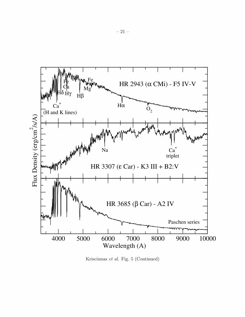
Fully reduced spectra, transformed to the “Sirius system” and ranging from 3300 to

10,000 A, are shown in Fig. 5. Spectra taken with only the blue grating are shown in

Fig. 6.8

6One must use a model spectrum of appropriate resolution. Otherwise the final spectra may contain

spurious features such as fictitious P Cygni profiles. A scaled FITS version of the Kurucz model spectrum

can be obtained via http://www.stsci.edu/hst/observatory/crds/calspec.html as file sirius mod 002.fits. A

comment in the header of this file indicates that fluxes have been scaled by 2.75440 ×10−16. This accounts

for the distance to Sirius and its limb-darkened angular diameter.

7 http://classic.sdss.org/dr7/products/spectra/vacwavelength.html

8 FITS and ASCII spectra are available via http://people.physics.tamu.edu/krisciunas/spec.tar.gz and

from the online version of this paper.

– 6 –

Some line identifications are given in the last panel of Fig. 5. In spectra of stars

hotter than the Sun we clearly see the Balmer lines at 6563, 4861, 4340, 4102 A and shorter

wavelengths. Cooler stars such as HR 3307 (ε Car) and HR 2061 (α Ori) show the infrared

Ca+ triplet (8498, 8542, and 8662 A) and the blended Na D lines (5890 and 5896 A). ζ Ori

and early B-type stars, such as HR 1790 (γ Ori), HR 2294 (β CMa), HR 2618 (ε CMa), and

HR 4853 (β Cru), show He I absorption at 4471 and 5876 A, though it is difficult to see

given the scale of the spectra shown in Figs. 5 and 6. A higher resolution spectrum of ζ

Ori A from 3980 to 4940 A, including line identifications, is shown in Fig. 14 of Soto et al.

(2011).

One thing to note in our reduced spectra is the strength of the Balmer jump in early-

type main sequence stars. This is due to ionization of atomic hydrogen from the first excited

state, producing strong absorption shortward of the Balmer limit at 3646 A. This results

in fainter U -band magnitudes of such stars. A much weaker Balmer jump is seen in hot

giant and supergiant stars. Thus, the Balmer jump gives us a photometric tool to measure

a combination of the luminosity class and the local acceleration of gravity of hot stars (log

g). For example, an A2 V star is 0.30 mag redder in the U − B color index than an A2 III

star (Drilling & Landolt 2000, pp. 388-389). Kaler (1962) points out that one also needs the

rotation rates of the stars to do this properly.

4. Synthetic Photometry

The filter prescriptions originally given by Bessell (1990) have been slightly modified

by Bessell & Murphy (2012). We have adopted the latter. In Fig. 7 we show their filter

prescriptions, multiplied by an atmospheric extinction function appropriate to Cerro Tololo,

and also multiplied by a function which accounts for the principal atmospheric extinction

lines. This is noticeable in the R- and I-band functions.

We then calculated synthetic BV RI magnitudes of our target stars using an iraf script

written by one of us (N. B. S.). This script uses an arbitrary zero point for each filter. We

adjusted the BV RI zero points to given synthetic magnitudes of the scaled Sirius model

spectrum that match those of Cousins (1971, 1980). If the reader chooses to adopt different

BV RI magnitudes of Sirius than those given in Table 1, then the synthetic magnitudes of

the other stars given in the table must be adjusted up or down accordingly.

Bessell and Murphy’s V -band filter prescription extends to 7400 A, while our blue

grating spectra stop at ∼6400 A. We cannot obtain synthetic V -band magnitudes for the

cooler stars observed only with the blue grating. However, we can obtain approximate V -

– 7 –

band magnitudes for the hot stars HR 2618, 3485, 4853, and 4963 by extrapolating the

spectra using the Rayleigh-Jeans approximation.

Table 1 gives our synthetic BV RI photometry. Fig. 8 shows the differences of our

synthetic photometry and the values of Cousins (1971) and Cousins (1980), as a function

B − V (for B and V ), V − R (for R), and V − I (for I). There is no color term for the

V -band differences, but there are non-zero colors terms for B, R, and I. At zero color there

is no offset between our V -band magnitudes and those of Cousins, but in B, R, and I ours

are 0.02 to 0.03 mag fainter.

From the AAVSO online light curve calculator we find that the V -band brightness of

α Ori was V = 0.398 on 2 January 2003, and V = 0.384 on 7 January. The mean is V =

0.391, which is comparable to our synthetic V -band magnitude of 0.398 from spectra taken

on 6 January 2003. This is a good sanity check. On 21 January 2005, when we took the red

grating spectra, Betelgeuse’s brightness was V = 0.436, according to the AAVSO.

The spectra presented here and the associated synthetic photometry can function as a

Sirius-based anchor for Galactic as well as extragalactic observational astronomy.

We made use of the SIMBAD database, operated at CDS, Strasbourg, France. We

thank the AAVSO for the V -band photometry of Betelgeuse obtained from their database.

Kenneth Luedeke and Raymond Thompson measured Betelgeuse closest to the times we took

spectra. We thank Ralph Bohlin for providing an ASCII version of the Kurucz spectrum of

Sirius used for the calibration, and for useful comments. We also thank James Kaler and

Jesus Maız Apellaniz for comments and references.

A. Other Spectra

The spectra shown in Figs. 5 and 6 were taken under demonstrably clear sky conditions.

Synthetic photometry based on these spectra is transformable to the systems of Cousins

(1971) and Cousins (1980) with uncertainties of ±0.03 mag or less. Other spectra were

taken which might be of use to the reader.

In Fig. 9 we show blue grating spectra of HR 5056 (α Vir) and HR 5267 (β Cen) taken

on 6 January 2003. For reasons that are not entirely clear, our synthetic photometry was

too faint by ∼0.55 mag and ∼0.12 mag for these two stars. The most likely explanation

is a misalignment of the telescope and the dome slit. We have scaled these two spectra by

appropriate amounts to make them consistent with photometry of Cousins (1971).

– 8 –

In Fig. 10 we show red grating spectra of HR 3454 (η Hya), HR 4216 (µ Vel), and HR

4450 (ξ Hya), taken through clouds on 21 January 2005. The spectra have been scaled to

make them consistent with photometry of Cousins (1980).

Finally, in Fig. 11 we show two spectra of η Carinae taken through clouds on 21 January

2005. The top spectrum is a coadd of 12 exposures of 7 seconds. Such a short exposure

time was necessary to prevent saturation of the H-α line. The bottom spectrum is a coadd

of 3 exposures of 240 seconds. In this spectrum H-α is saturated, but other emission lines

such as the Paschen lines of hydrogen and multiple helium lines are evident with a better

signal-to-noise ratio. Since η Car has such a non-stellar spectrum and we have no available

R- or I-band photometry of this star at this epoch, we have not scaled our spectra like the

others presented in this Appendix.

These additional spectra are available from the first author of this article.

– 9 –

REFERENCES

Bessell, M. S. 1990, PASP, 102, 1181

Bessell, M. S. & Murphy, S. 2012, PASP, 124, 140

Bohlin, R. C. 2014, AJ, 147, 127

Bohlin, R. C., Gordon, K. D., & Tremblay, P.-E. 2014, PASP, 126, 711

Bohlin, R. C., & Landolt, A. U. 2015, AJ, 149, 122

Butkovskaya, V. V. 2014, Bull. Crimean Astrophys. Obs. 110, 80

Cousins, A. W. J. 1971, Roy. Obs. Annals, 7, 1

Cousins, A. W. J. 1980, South Afr. Astr. Obs. Circular, 1, 234

Drilling, J. S. & Landolt, A. U. 2000, in Allen’s Astrophysical Quantities, 4th ed., A. N.

Cox, ed., New York, Berlin, Heidelberg: Springer, pp. 381-396

Fukugita, M., Ichikawa, T., Gunn, J. E., Doi, M., Shimasaku, K., & Schneider, D. P. 1996,

AJ, 111, 1748

Hamuy, M., Walker, A. R., Suntzeff, N. B., Gigoux, P., Heathcote, S. R., & Phillips, M. M.

1992, PASP, 104, 533

Hamuy, M., Suntzeff, N. B., Heathcote, S. R., Walker, A. R., Gigoux, P., & Phillips, M. M.

1994, PASP, 106, 566

Hayes, D. S., & Latham, D. W. 1975, ApJ, 197, 593

Hearnshaw, J. B. 1996, The Measurement of Starlight: Two Centuries of Astronomical Pho-

tometry, Cambridge: Cambridge Univ. P.

Hearnshaw, J. B. 2014, The Analysis of Starlight: Two Centuries of Astronomical Spec-

troscopy, 2nd ed., Cambridge: Cambridge Univ. P.

Johnson, H. L., & Morgan, W. W. 1953, ApJ, 117, 313

Kaler, J. 1962, Zeitschrift fur Astrophys., 56, 150

Krisciunas, K. 1982, IBVS 2104

Krisciunas, K., & Fisher, D. 1988, IBVS 3227

– 10 –

Krisciunas, K. 1990, IBVS 3477

Krisciunas, K., & Luedeke, K. D. 1996, IBVS 4355

Massey, P., Valdes, F., & Barnes, J. 1992, A User’s Guide to Reducing Slit Spectra with

IRAF

Soto, A., Maız Apellaniz, J., Walborn, N. R., Alfaro, E. J., Barba, R. H., Morrell, N. I.,

Gamen, R. C., & Arias, J. I. 2011, ApJS, 193, 24

Stritzinger, M., Suntzeff, N. B., Hamuy, M., Challis, P., Demarco, R., Germany, L., &

Soderberg, A. M. 2005, PASP, 117, 810

Su, K. Y. L., Rieke, G. H., Misselt, K. A., et al. 2005, ApJ, 628, 487

Su, K. Y. L., Rieke, G. H., Malhotra, R., et al. 2013, ApJ, 763, 118

Tompkin, J. 1998, Sky and Telescope, 95, no. 4, 59

This preprint was prepared with the AAS LATEX macros v5.2.

– 11 –

Tab

le1.

Synth

etic

Phot

omet

ryof

Tar

get

Sta

rs

HR

aName

Binary/Multiple?

SpectralTypeb

Xblu

ec

Xredd

BV

RI

1544

π2Ori

NA1Vn

1.338

1.427

4.381

4.365

4.365

4.351

1713

βOri

NB8Ia:

1.085

1.144

0.200

0.224

0.173

0.148

1790

γOri

NB2III

1.253

1.352

1.425

1.635

1.756

1.888

1948/1949

ζOri

A/B

YO9.7b+O9III+

B0II-IV

1.376

1.223

1.635

1.826

1.874

1.968

2061e

αOri

NM1-2

Ia-Iab

1.291

1.321

2.198

0.398

−0.653−1.799

2294

βCMa

NB1II-III

1.316

1.123

1.761

1.996

2.126

2.265

2326

αCar

NF0II

1.251

1.137−0.584−0.726−0.830−0.952

2491f

αCMa

YA1V

1.123

1.077−1.425−1.420−1.408−1.400

2943

αCMi

YF5IV

-V1.299

1.226

0.761

0.357

0.132

−0.098

3307

εCar

YK3III+

B2:V

1.211

1.147

3.081

1.844

1.092

0.360

3685

βCar

NA2IV

1.428

1.305

1.674

1.661

1.693

1.690

99

αPhe

YK0III

1.562

...

3.460

...

...

...

2618

εCMa

YB2II

1.226

...

1.315

1.519

...

...

2693

δCMa

NF8Ia

1.172

...

2.533

...

...

...

3485

δVel

YA1V

1.177

...

1.990

1.949

...

...

3634

λVel

NK4.5

Ib-II

1.126

...

3.822

...

...

...

3748

αHya

NK3II-III

1.126

...

3.415

...

...

...

4763

γCru

NM3.5

III

1.192

...

3.160

...

...

...

4853

βCru

YB0.5

III

1.169

...

1.050

1.241

...

...

4963

θVir

YA1IV

s+Am

1.225

...

4.392

4.364

...

...

Note.—

Thestars

listed

inth

etop

half

ofth

etable

wereobserved

with

thebluegratingand

thered

grating.Thestars

inth

e

bottom

halfofth

etable

wereonly

observed

withth

ebluegrating.

aHarvard

Rev

ised

number

=ca

talognumber

inTheBrigh

tStarCatalogu

e.

bFrom

onlineversionofTheBrigh

tStarCatalogu

e,5th

edition,1991.

cMea

nairmass

forbluegratingsp

ectraobtained

on6January

2003UT.

dMea

nairmass

forredgratingsp

ectraobtained

on21January

2005UT.

eα

Ori

isvariable.See

textforco

mmen

ts.

fBV

photometry

from

Cousins(1971).RIphotometry

from

Cousins(1980).

– 12 –

Fig. 1.— Positions of our target stars on the sky. The numerical labels are the catalog

numbers in The Bright Star Catalogue. Blue dots represent stars that were observed with

the blue grating only. Other stars were observed with both the blue and red gratings.

Fig. 2.— V -band magnitude of α Ori from October 1979 through November 1996. Key to

data points: blue dots (K. Krisciunas), green squares (D. Fisher), red triangles (K. Luedeke).

Data by Fisher were published by Krisciunas & Fisher (1988). Data by Luedeke were pub-

lished by Krisciunas & Luedeke (1996).

Fig. 3.— Instrumental magnitudes of Sirius vs. airmass on 6 January 2003 (UT). The Y-axis

values are equal to −2.5 log10 of the integrated counts from 3600 to 5500 A of spectra that

have only been wavelength-calibrated.

Fig. 4.— Top: Kurucz model spectrum of Sirius with R = 1000, T = 9850 K, log g =

4.30, and [Fe/H] = +0.4. Middle: Average of calibrated Sirius spectra taken with airmass

less than 1.3. This is the output from iraf. Bottom: Ratio of model spectrum of Sirius to

output from iraf. This is the “flux function” or “spectral flat” used to multiply the reduced

spectra of the other stars to place the spectra on the system of the Kurucz model of Sirius.

In the bottom two panels the Fraunhofer B, A, and Z lines at 6867, 7594, and 8227 A are

labeled. These are due to molecular oxygen in the Earth’s atmosphere.

Fig. 5.— Spectra of program stars observed with the blue grating and the red grating.

Small spurious variations of the flux density are seen in some spectra at 6000 and ∼7600

A which are attributable to the method of construction of the “spectral flat”. Some line

identifications are given in the last panel of this figure. See text for further information.

Fig. 6.— Spectra of program stars observed with the blue grating only.

Fig. 7.— Fractional transmission of Bessell & Murphy (2012) filters, multiplied by an at-

mospheric extinction model appropriate to Cerro Tololo, and also multiplied by a function

that accounts for principal terrestrial atmospheric features. As our spectra are not useful

shortward of 3300 A, designated here by a vertical dashed line, we can not easily obtain

U -band synthetic photometry of our program stars.

Fig. 8.— Differences of photometry in the sense “our synthetic photometry” minus “pho-

tometry of Cousins”. The slope is also known as the “color term”.

Fig. 9.— Spectra of HR 5056 (α Vir) and HR 5267 (β Cen) obtained on 6 January 2003.

Fig. 10.— Spectra of HR 3454 (η Hya), HR 4216 (µ Vel), and HR 4450 (ξ Hya) obtained on

21 January 2005 under non-photometric conditions.

– 13 –

Fig. 11.— Spectra of η Carinae, obtained under non-photometric conditions on 21 January

2005. Top: Coadd of shorter exposures. The H-α line is not saturated. Bottom: Coadd of

longer exposures. While the H-α line is saturated, other spectral features are more easily

seen.

– 14 –

02468101214Right Ascension (hours)

-80

-70

-60

-50

-40

-30

-20

-10

0

10

20

Dec

linat

ion (

deg

)

99

1544

1713

1790

1948

2061

2294Sirius

2326

2943

3307

3685

2618

2693

3485

3634

3748

4763

4853

4963

Krisciunas Fig. 1.

– 15 –

4000 4500 5000 5500

0.2

0.4

0.6

0.8

1

V

6000 6500 7000

0.2

0.4

0.6

0.8

1

V

7500 8000 8500

0.2

0.4

0.6

0.8

1

V

9000 9500 10000

Julian Date [2,440,000 + ...]

0.2

0.4

0.6

0.8

1

V

α Ori

Krisciunas Fig. 2.

– 16 –

1 1.1 1.2 1.3 1.4 1.5 1.6 1.7 1.8 1.9 2 2.1Air mass

-17.05

-17

-16.95

-16.9

-16.85

-16.8

-16.75

-16.7

Inst

rum

enta

l m

agnit

ude

slope = 0.237 +/- 0.009

RMS = +/− 0.018

6 January 2003 (UT)

Krisciunas Fig. 3.

– 17 –

0

1e-08

2e-08

3e-08

4e-08

0

1e-08

2e-08

3e-08

4e-08

5e-08

Flu

x D

ensi

ty (

erg

/cm

2/s

/A)

4000 5000 6000 7000 8000 9000 10000Wavelength (A)

0

0.5

1

1.5

Rat

io

Kurucz model

T = 9850 log g = 4.30 [Fe/H] = +0.4

Sirius spectrum (output of IRAF)

Ratio

B A Z?

?

B

A

Z

Krisciunas Fig. 4.

– 18 –

4000 5000 6000 7000 8000 9000 10000Wavelength (A)

0

5e-11

1e-10

1.5e-10

2e-10

Flu

x D

ensi

ty (

erg/c

m2/s

/A)

HR 1544 (π2

Ori) - A1 Vn

Krisciunas et al. Fig. 5

– 19 –F

lux D

ensi

ty (

erg/c

m2/s

/A)

4000 5000 6000 7000 8000 9000 10000Wavelength (A)

HR 1713 (β Ori) - B8 Ia:

HR 1790 (γ Ori) - B2 III

HR 1948/1949 (ζ Ori Aa +Ab +B) -

O9.7 Ib + O9 III + B0 II-IV

Krisciunas et al. Fig. 5 (Continued)

– 20 –F

lux D

ensi

ty (

erg/c

m2/s

/A)

4000 5000 6000 7000 8000 9000 10000Wavelength (A)

HR 2061 (α Ori) - M1-2 Ia-Iab

HR 2294 (β CMa) - B1 II-III

HR 2326 (α Car) - F0 II

Krisciunas et al. Fig. 5 (Continued)

– 21 –F

lux D

ensi

ty (

erg/c

m2/s

/A)

4000 5000 6000 7000 8000 9000 10000Wavelength (A)

HR 2943 (α CMi) - F5 IV-V

HR 3307 (ε Car) - K3 III + B2:V

HR 3685 (β Car) - A2 IV

Hα

HβHγ

FeCa

Ca+

(H and K lines)O

2

Hδ

Na Ca+

triplet

Mg

Fe

Paschen series

Krisciunas et al. Fig. 5 (Continued)

– 22 –F

lux D

ensi

ty (

erg/c

m2/s

/A)

3500 4000 4500 5000 5500 6000 6500Wavelength (A)

HR 99 (α Phe) - K0 III

HR 2618 (ε CMa) - B2 II

HR 2693 (δ CMa) - F8 Ia

Krisciunas et al. Fig. 6

– 23 –F

lux D

ensi

ty (

erg/c

m2/s

/A)

3500 4000 4500 5000 5500 6000 6500Wavelength (A)

HR 3485 (δ Vel) - A1 V

HR 3634 (λ Vel) - K4.5 Ib-II

HR 3748 (α Hya) - K3 II-III

Krisciunas et al. Fig. 6 (Continued)

– 24 –F

lux D

ensi

ty (

erg/c

m2/s

/A)

3500 4000 4500 5000 5500 6000 6500Wavelength (A)

HR 4763 (γ Cru) - M3.5 III

HR 4853 (β Cru) - B0.5 III

HR 4963 (θ Vir) - A1 IV s+Am

Krisciunas et al. Fig. 6 (Continued)

– 25 –

3000 4000 5000 6000 7000 8000 9000Wavelength (A)

0

0.2

0.4

0.6

0.8

1

Fra

ctio

nal

tra

nsm

issi

on

U

B

V R

I

Krisciunas Fig. 7.

– 26 –

0 0.5 1 1.5 2B − V

-0.2

-0.15

-0.1

-0.05

0

0.05

0.1

0.15

0.2

∆ B

0 0.5 1 1.5 2B − V

-0.2

-0.15

-0.1

-0.05

0

0.05

0.1

0.15

0.2

∆ V

0 0.5 1 1.5 2V − R

-0.2

-0.15

-0.1

-0.05

0

0.05

0.1

0.15

0.2

∆ R

0 0.5 1 1.5 2 2.5V − I

-0.2

-0.15

-0.1

-0.05

0

0.05

0.1

0.15

0.2

∆ I

slope = −0.042 +/− 0.008

RMS = +/− 0.027

slope = −0.017 +/− 0.009

RMS = +/- 0.020

slope = −0.002 +/− 0.011

RMS = +/− 0.013

slope = +0.030 +/− 0.007

RMS = +/− 0.017

Krisciunas Fig. 8.

– 27 –(e

rg/c

m2/s

/A)

3500 4000 4500 5000 5500 6000 6500Wavelength (A)

Flu

x D

ensi

ty

HR 5056 (α Vir) - B1 III-IV + B2 V

HR 5267 (β Cen) - B1 III

Krisciunas Fig. 9.

– 28 –F

lux D

ensi

ty (

erg/c

m2/s

/A)

6000 7000 8000 9000 10000Wavelength (A)

HR 3454 (η Hya) - B3 V

HR 4216 (µ Vel) - G5 III + G2 V

HR 4450 (ξ Hya) - G7 III

Krisciunas Fig. 10.

– 29 –(e

rg/c

m2/s

/A)

5500 6000 6500 7000 7500 8000 8500 9000Wavelength (A)

Flu

x D

ensi

ty

HR 4210 (η Car)

exptime = 12 X 7 sec

exptime = 3 X 240 sec

Krisciunas Fig. 11.