spectral three-term conjugate descent method for …

ISSN 1686-0209

Thai Journal of MathematicsVol. 18, No. 1 (2020),

Pages 501 - 517

SPECTRAL THREE-TERM CONJUGATE DESCENT

METHOD FOR SOLVING NONLINEAR MONOTONE

EQUATIONS WITH CONVEX CONSTRAINTS

Auwal Bala Abubakar, 1∗, Jewaidu Rilwan1, Seifu Endris Yimer,2, Abdulkarim Hassan Ibrahim 4, IdrisAhmed 3

1Department of Mathematical Sciences, Faculty of Physical Sciences, Bayero University, Kano. Kano, Nigeria.2Department of Mathematics, College of Computation and Natural Science , Debre Berhan University, P.O.Box 445, Debre Berhan , Ethiopia.3Department of Mathematics and Computer Science, Faculty of Natural and Applied Sciences , Sule LamidoUniversity Kafin Hausa, P.M.B 048, Jigawa State, Nigeria.4Department of Mathematics, Faculty of Science, King Mongkut’s University of Technology Thonburi(KMUTT), 126 Pracha Uthit Road, Bang Mod,Thung Khru, Bangkok 10140, Thailand.Email addresses: [email protected] (A. B. Abubakar), [email protected] (J. Rilwan),[email protected] (S. E. Yimer), [email protected] (A. H. Ibrahim),[email protected] (I. Ahmed)

Abstract This paper proposes three (3) three term conjugate gradient (CG) methods based on the well

known conjugate descent (CD) CG parameter. The two directions were obtained by adding a term to

the CD direction such that the sufficient descent property is satisfied. Under some assumptions, we

establish the convergence of the proposed methods. In addition, numerical examples were given to show

the capability of the two methods in solving nonlinear monotone equations with convex constraints.

MSC: 65K05; 90C52; 90C56; 92C55

Keywords: Nonlinear monotone equations, Conjugate gradient method, Projection method

Submission date: 30.11.2019 / Acceptance date: 18.02.2020

1. Introduction

A nonlinear monotone equation with convex constraints is an equation of the form

F (x) = 0, subject to x ∈ Ω, (1.1)

where F : Rn → Rn is continuous and monotone. The set Ω ⊂ Rn is assumed to benonempty, closed and convex.

The above problem feature in many applications, such as the subproblems in the gen-eralized proximal algorithms with Bregman distance [1], reformulation of ℓ1-norm reg-ularized problems [2], and conversionn of variational inequality problems into nonlinearmonotone equations via fixed point maps [3].

*Corresponding author. Published by The Mathematical Association of Thailand.Copyright c⃝ 2020 by TJM. All rights reserved.

502 Thai J. Math. Vol. 18, No. 1 (2020) / Abubakar et al.

Among famous and efficient methods for solving (1.1) are the conjugate gradient (CG)methods. They are iterative methods for solving unconstrained optimization problem andnonlinear systems, due to low memory requirement (see [4–10] and references their in).This and other reasons inspired many authors to propose CG methods combined withthe projection method by Solodov and Svaiter [11].

Given an initial guess xk, the conjugate gradient algorithm combined with the projec-tion method computes the next guess xk+1 as

xk+1 = PΩ[xk − ζkF (zk)] (1.2)

where

PΩ(x) = argmin∥x− y∥ : y ∈ Ω.,

ζk = F (zk)T (xk−zk)

∥F (zk)∥2 and zk = xk + αkdk. αk is the step size obtained using a suitable line

search procedure and the search direction

dk =

−F (xk), if k = 0,

−F (xk) + βkdk−1, if k ≥ 1,(1.3)

with βk being the conjugate gradient parameter. An important condition needed for thedirection to satisfy is

F (xk)T dk ≤ −c∥F (xk)∥2, c > 0. (1.4)

This condition ensures a decrease in the norm of the residual at each iteration. A niceproperty of the projection map is it’s nonexpansiveness, that is

∥PΩ(x)− PΩ(y)∥ ≤ ∥x− y∥, ∀x, y ∈ Rn. (1.5)

Among such methods are the two directions proposed by Ahookhosh et al. [12]. Thesearch directions are defined as

dk =

−F (xk), if k = 0,

−F (xk) + βPRPk wk−1 − θikyk−1, if k ≥ 1 and i=1,2,

(1.6)

where

βPRPk =

F (xk)T yk−1

∥F (xk−1)∥2,

θ1k =F (xk)

T yk−1∥wk−1∥2

∥F (xk−1)∥4,

θ2k =F (xk)

Twk−1

∥F (xk−1)∥2+

F (xk)T yk−1∥yk−1∥2

∥F (xk−1)∥4,

yk−1 = F (xk)− F (xk−1), wk−1 = zk−1 − xk−1 = αk−1dk−1.

The global convergence was established under the line search

−F (zk)T dk ≥ σαk∥F (zk)∥∥dk∥2, σ > 0. (1.7)

Another is that proposed by Papp and Rapajic [13] which is modified Fletcher-Reeves(FR) CG method. The directions are defined as

dk =

−F (xk), if k = 0,

−F (xk) + βFRk wk−1 − θikF (xk), if k ≥ 1 and i=1,2,3,

(1.8)

SPECTRAL THREE-TERM CONJUGATE DESCENT METHOD . . . 503

where

βFRk =

∥F (xk)∥2

∥F (xk−1)∥2,

θ1k =F (xk)

Twk−1

∥Fk−1∥2,

θ2k =∥F (xk)∥2∥wk−1∥2

∥∥F (xk−1)∥∥4,

θ3k =F (xk)

Twk−1

∥∥F (xk−1)∥∥2+

∥F (xk)∥2

∥∥F (xk−1)∥∥4.

The three directions based on θ1k, θ2k, and θ3k are called M3TFR1, M3TFR2 and M3TFR3

respectively. Numerical results presented reveals that overall, M3TFR1 has the leastnumber of iterations. However, in terms of number of function evaluations and CPUtime, M3TFR2 was the most efficient and robust.Likewise, Feng et al. [14] proposed a search direction given by

dk =

−F (xk), if k = 0,

−(1 + βk

F (xk)T dk−1

∥F (xk)∥2

)F (xk) + βkdk−1, if k ≥ 1,

(1.9)

where βk = ∥F (xk)∥∥dk−1∥ .

The global convergence was proved using the line search

−F (zk)T dk ≥ σαk∥dk∥2, σ > 0. (1.10)

. Just recently, Abubakar et. al [15] proposed a modified version of the method proposedby [13] defined as

dk =

−F (xk), if k = 0,

−F (xk) +∥F (xk)∥2wk−1−F (xk)

Twk−1F (xk)maxµ∥wk−1∥∥F (xk)∥,∥F (xk−1)∥2 , if k ≥ 1,

(1.11)

where µ > 0 is a positive constant. The difference between the M3TFR1 direction andthe above direction is the scaling term appearing in the denominator of Equation (1.11).To have more incite on conjugate gradient projection methods, the reader is referred to[16–22].

Motivated by the above methods and in particular the method proposed in [12, 13],we present three spectral conjugate descent projection methods. Section 2 gives detail ofthe proposed methods. In Section 3, the global convergence of the proposed methods isdiscussed. Numerical experiments are carried out in section 4. Finally section 5 has theconclusion.

2. Algorithm: Inspiration and convergence analysis

We begin this section by defining the projection map, then introduce our proposedmethod together with is convergence analysis.

Definition 2.1. Let Ω ⊂ Rn be a nonempty closed convex set. Then for any x ∈ Rn, itsprojection onto Ω, denoted by PΩ(x), is defined by

PΩ(x) = argmin∥x− y∥ : y ∈ Ω.


Indeed, PΩ is nonexpansive, That is,

∥PΩ(x)− PΩ(y)∥ ≤ ∥x− y∥, ∀x, y ∈ Rn. (2.1)

All through, we assume the followings

(K1) The function F is monotone, that is,

(F (x)− F (y))T (x− y) ≥ 0, ∀x, y ∈ Rn.

(K2) The function F is Lipschitz continuous, that is there exists a positive constantL such that

∥F (x)− F (y)∥ ≤ L∥x− y∥, ∀x, y ∈ Rn.

(K3) The solution set of (1.1), denoted by Ω, is nonempty.

An important property that is required of a method for solving equation (1.1) to possessis that the direction dk satisfy

F (xk)T dk ≤ −δ∥F (xk)∥2, (2.2)

where δ > 0. The above relation (2.2) is called the sufficient descent condition if F (x) isthe gradient vector of a real valued function f : Rn → R.

Inspired by the directions proposed in [12] and [13], we propose the following searchdirection

dk =

−F (xk), if k = 0,

−F (xk) + βCDk wk−1 − λkF (xk), if k ≥ 1,

(2.3)

where

βCDk =

∥F (xk)∥2

−dTk−1F (xk−1), (2.4)

wk−1 = zk−1 − xk−1 = αk−1dk−1. The parameter λk will be derived in three differentapproaches such that (2.2) is satisfied.M3TCD1 direction: Multiplying (2.3) by F (xk)

T and substituting (2.4) in (2.3), wehave

F (xk)T dk = −∥F (xk)∥2 +

∥F (xk)∥2

−dTk−1F (xk−1)F (xk)

Twk−1 − λk∥F (xk)∥2.

By choosing

λk =F (xk)

Twk−1

−dTk−1F (xk−1), (2.5)

then (2.2) is satisfied with δ = 1, that is F (xk)T dk = −∥F (xk)∥2.

we call the first modified three term CD like direction M3TCD1 which is defined by(2.3),(2.4) and (2.5).M3TCD2 direction: Applying similar approach used in [12] and [13], we have

F (xk)T dk

=[− ∥F (xk)∥2(dTk−1F (xk−1))

2 − dTk−1F (xk−1)∥F (xk)∥2

× F (xk)Twk−1 − λk∥F (xk)∥2(dTk−1F (xk−1))

2]/(dTk−1F (xk−1))

2.


Using the relation uT v ≤ 12 (∥u∥

2 + ∥v∥2) and letting u = − 1√2(dTk−1F (xk−1))F (xk) and

v =√2∥F (xk)∥2wk−1, then

F (xk)T dk

=[− ∥F (xk)∥2(dTk−1F (xk−1))

2 +1

4(dTk−1F (xk−1))

2∥F (xk)∥2

+ ∥F (xk)∥4∥wk−1∥2 − λk∥F (xk)∥2(dTk−1F (xk−1))2]/(dTk−1F (xk−1))

2

= −∥F (xk)∥2 +1

4∥F (xk)∥2 +

∥F (xk)∥4∥wk−1∥2

(dTk−1F (xk−1))2− λk∥F (xk)∥2

= −3

4∥F (xk)∥2 +

∥F (xk)∥4∥wk−1∥2

(dTk−1F (xk−1))2− λk∥F (xk)∥2.

(2.6)

Choosing

λk =∥F (xk)∥2∥wk−1∥2

(dTk−1F (xk−1))2, (2.7)

then then (2.2) is satisfied with δ = 34 , that is F (xk)

T dk = − 34∥F (xk)∥2. The direction

defined by (2.3),(2.4) and (2.7) is called M3TCD2.M3TCD3 direction: This third parameter λk is chosen as

λk =F (xk)

Twk−1

−dTk−1F (xk−1)+

∥F (xk)∥2

(dTk−1F (xk−1))2. (2.8)

The first term is (2.5) and the second term is chosen such that (2.2) is satisfied. Now,multiplying (2.3) by F (xk)

T and substituting (2.4) and (2.8) in (2.3), we have

F (xk)T dk = −∥F (xk)∥2 +

∥F (xk)∥2


Twk−1

−

(F (xk)

Twk−1


∥F (xk)∥2

(dTk−1F (xk−1))2

)∥F (xk)∥2

= −∥F (xk)∥2 −∥F (xk)∥4

(dTk−1F (xk−1))2

≤ −∥F (xk)∥2.

The above relation shows that (2.2) is satisfied with δ = 1. We call the direction definedby (2.3), (2.4) and (2.8) M3TCD3.

To prove the global convergence of Algorithm 1, the following lemmas are needed.

Lemma 2.2. The directions M3TCD1, M3TCD2 and M3TCD3 by satisfy the sufficientdescent condition (2.2).

Remark 2.3. Since M3TCD1, M3TCD2 and M3TCD3 by satisfy the sufficient descentcondition (2.2) ∀k ∈ N

∪0, then

F (xk−1)T dk−1 ≤ −δ∥F (xk−1)∥2,

which implies

1

−F (xk−1)T dk−1≤ 1

δ∥F (xk−1)∥2(2.10)


Algorithm 1

Step 0. Given an arbitrary initial point x0 ∈ Rn, parameters σ > 0, 0 < ρ < 1, Tol > 0and set k := 0.

Step 1. If ∥F (xk)∥ ≤ Tol, stop, otherwise go to Step 2.Step 2. Compute dk using Equation (2.3).

Step 3. Compute the step size αk = maxγρi : i = 0, 1, 2, · · · such that

−F (xk + αkdk)T dk ≥ σαk∥F (xk + αkdk)∥∥dk∥2. (2.9)

Step 4. Set zk = xk + αkdk. If zk ∈ Ω and ∥F (zk)∥ ≤ Tol, stop. Else compute

xk+1 = PΩ[xk − ζkF (zk)]

where

ζk =F (zk)

T (xk − zk)

∥F (zk)∥2.

Step 5. Let k = k + 1 and go to Step 1.

Lemma 2.4. Suppose assumptions (K1)-(K3) holds, xk and zk defined by Algorithm1. Then

αk ≥ max

γ,

ρδ∥F (xk)∥(L+ σ∥F (xk + αkdk)∥)∥dk∥2

. (2.11)

Proof. By the line search (2.9), if αk = γ, the α′

k = αkρ−1 does not satisfy (2.9), that is

−F (xk + α′

kdk)T dk < σα

′

k∥F (xk + α′

kdk)∥∥dk∥2.

Now from (2.2) and assumption (K2), we have

δ∥F (xk)∥2 ≤ −F (xk)T dk

= (F (xk + α′

kdk)− F (xk))T dk − F (xk + α

′

kdk)T dk

≤ α′

k(L+ σ∥F (xk + αkdk)∥)∥dk∥2.

The desired result is obtained after solving for α′

k.

Lemma 2.5. Suppose assumptions (K1)-(K3) holds, then xk and zk defined by Al-gorithm 1 are bounded. In addition, we have

limk→∞

∥xk − zk∥ = 0 (2.12)

and

limk→∞

∥xk+1 − xk∥ = 0. (2.13)

Proof. We will start by showing that the sequences xk and zk are bounded. Supposex ∈ Ω, then by monotonicity of F , we get

F (zk)T (xk − x) ≥ F (zk)

T (xk − zk). (2.14)

Also by definition of zk and the line search (2.9), we have

F (zk)T (xk − zk) ≥ σα2

k∥F (zk)∥∥dk∥2 ≥ 0. (2.15)


So, we have

∥xk+1 − x∥2 = ∥PΩ[xk − ζkF (zk)]− x∥2 ≤ ∥xk − ζkF (zk)− x∥2

= ∥xk − x∥2 − 2ζkF (zk)T (xk − x) + ∥ζF (zk)∥2

≤ ∥xk − x∥2 − 2ζkF (zk)T (xk − zk) + ∥ζF (zk)∥2

= ∥xk − x∥2 −(F (zk)

T (xk − zk)

∥F (zk)∥

)2

≤ ∥xk − x∥2

(2.16)

Thus the sequence ∥xk − x∥ is decreasing and convergent, and hence xk is bounded.Furthermore, from equation (2.16), we have

∥xk+1 − x∥2 ≤ ∥xk − x∥2, (2.17)

and we can conclude recursively that

∥xk − x∥2 ≤ ∥x0 − x∥2, ∀k ≥ 0.

Then from Assumption (G2), we obtain

∥F (xk)∥ = ∥F (xk)− F (x)∥ ≤ L∥xk − x∥ ≤ L∥x0 − x∥.

If we let L∥x0 − x∥ = M , then the sequence F (xk) is bounded, that is,

∥F (xk)∥ ≤ M, ∀k ≥ 0. (2.18)

By the definition of zk, equation (2.15), monotonicity of F and the Cauchy-Schwatzinequality, we get

σ∥xk − zk∥ =σ∥αkdk∥2

∥xk − zk∥≤ F (zk)

T (xk − zk)

∥xk − zk∥≤ F (zk)

T (xk − zk)

∥xk − zk∥≤ ∥F (xk)∥.

(2.19)

The boundedness of the sequence xk together with equation (2.18)-(2.19), implies thesequence zk is bounded.

Since zk is bounded, then for any x ∈ Ω, the sequence zk− x is also bounded, thatis, there exists a positive constant ν > 0 such that

∥zk − x∥ ≤ ν.

This together with Assumption (G2) yields

∥F (zk)∥ = ∥F (zk)− F (x)∥ ≤ L∥zk − x∥ ≤ Lν.

Therefore, using equation (2.16), we have

σ2

(Lν)2∥xk − zk∥4 ≤ ∥xk − x∥2 − ∥xk+1 − x∥2,


which implies

σ2

(Lν)2

∞∑k=0

∥xk − zk∥4 ≤∞∑k=0

(∥xk − x∥2 − ∥xk+1 − x∥2) ≤ ∥x0 − x∥ < ∞. (2.20)

Equation (2.20) implies

limk→∞

∥xk − zk∥ = 0.

However, using Equation 2.1, the definition of ζk and the Cauchy-Schwartz inequality, wehave

∥xk+1 − xk∥ = ∥PΩ[xk − ζkF (zk)]− xk∥

≤ ∥xk − ζkF (zk)− xk∥

= ∥ζkF (zk)∥

= ∥xk − zk∥,

(2.21)

which yields

limk→∞

∥xk+1 − xk∥ = 0.

Equation (2.12) and definition of zk implies that

limk→∞

αk∥dk∥ = 0. (2.22)

Theorem 2.6. Suppose that assumptions (K1)-(K3) hold and let the sequence xk begenerated by Algorithm 1, then

lim infk→∞

∥F (xk)∥ = 0, (2.23)

Proof. Suppose by contradiction that (2.23) is not true, then there exist r0 > 0 such that∀k ≥ 0

∥F (xk)∥ ≥ r0. (2.24)

This combined with (2.2) yields

∥dk∥ ≥ δr0 ∀k ≥ 0. (2.25)


Next we will show that the directions M3TCD1, M3TCD2 and M3TCD3 are bounded.M3TCD1: Using (2.3), (2.4), (2.5), (2.10), (2.18) and (2.24), we have

∥dk∥ =

∥∥∥∥∥−F (xk) +∥F (xk)∥2

−dTk−1F (xk−1)wk−1 −

F (xk)Twk−1


∥∥∥∥∥≤ ∥F (xk)∥+ 2

∥F (xk)∥2∥wk−1∥δ∥F (xk−1)∥2

= ∥F (xk)∥+ 2∥F (xk)∥2αk−1∥dk−1∥

δ∥F (xk−1)∥2

≤ M +2M2

δr20αk−1∥dk−1∥.

(2.26)

Equation (2.22) implies that for all ϵ0 > 0 there exist k0 such that αk−1∥dk−1∥ < ϵ0for all k > k0. So choosing ϵ0 = r20 and κ = max∥d0∥, ∥d1∥, · · · , ∥dk0

∥,M1 whereM1 = M(1 + 2M

δ ). Therefore ∥dk∥ ≤ κ.M3TCD2 direction: Also by (2.3), (2.4), (2.7), (2.10), (2.18) and (2.24), we have

∥dk∥ =

∥∥∥∥∥−F (xk) +∥F (xk)∥2


∥F (xk)∥2∥wk−1∥2

(dTk−1F (xk−1))2F (xk)

∥∥∥∥∥≤ ∥F (xk)∥+

∥F (xk)∥2∥wk−1∥δ∥F (xk−1)∥2

+∥F (xk)∥3∥wk−1∥2

δ2∥F (xk−1)∥4

= ∥F (xk)∥+∥F (xk)∥2αk−1∥dk−1∥

δ∥F (xk−1)∥2+

∥F (xk)∥3(αk−1∥dk−1∥)2

δ2∥F (xk−1)∥4

≤ M +M2

δr20αk−1∥dk−1∥+

M3(αk−1∥dk−1∥)2

δ2r40.

(2.27)

In a similar way as above, letting κ = max∥d0∥, ∥d1∥, · · · , ∥dk0∥,M1 where M1 =M(1 + M

δ + (Mδ )2), we get that ∥dk∥ ≤ κ.


M3TCD3 direction: Again by (2.3), (2.4), (2.8), (2.10), (2.18) and (2.24), we have

∥dk∥ =

∥∥∥∥∥−F (xk) +∥F (xk)∥2


(F (xk)

Twk−1


∥F (xk)∥2

(dTk−1F (xk−1))2

)F (xk)

∥∥∥∥∥≤ ∥F (xk)∥+ 2

∥F (xk)∥2∥wk−1∥δ∥F (xk−1)∥2

+∥F (xk)∥3

δ2∥F (xk−1)∥4

= ∥F (xk)∥+ 2∥F (xk)∥2αk−1∥dk−1∥

δ∥F (xk−1)∥2+

∥F (xk)∥3

δ2∥F (xk−1)∥4

≤ M +M2

δr20αk−1∥dk−1∥+

M3

δ2r40.

(2.28)

Using same argument and letting κ = max∥d0∥, ∥d1∥, · · · , ∥dk0∥,M1 whereM1 = M(1+2Mδ + M2

δ2r40). Hence ∥dk∥ ≤ κ.

Now multiplying both sides of (2.11) with ∥dk∥, we have

αk∥dk∥ ≥ max

γ,

ρδ∥F (xk)∥(L+ σ∥F (xk + αkdk)∥)∥dk∥2

∥dk∥

≥ max

γδr0 ,

ρδr20L(1 + σν)κ

.

The above relation contradicts (2.22) and therefore (2.23) must hold.

3. Numerical Experiments

This section investigates the numerical performance of the proposed algorithms withother conjugate gradient algorithms.

We tested the following algorithms:

CGD: the algorithm proposed by Xiao and Zhu [23]

PCG: the algorithm proposed by Liu and Li [24]

M3TCD1: Algorithm 1 with the choice of λk using (2.5)



All algorithms were coded in MATLAB using a windows 10 operating system of 2.4GHzIntel(R) Core(TM) i3-7100U CPU with 8GB RAM. The experiments were carried outon eight benchmark test problems using seven initial points with dimension ranging from


n =5000 to 100000. Note that one of the initial points was randomly chosen. For the im-plementation of M3TCD1, M3TCD2 and M3TCD3, we choose the following parameters:σ = 10−4, ρ = 0.9 and γ = 1. We implemented CGD and PCG as in [23, 24].

The chosen stopping condition was

∥Fk∥ ≤ 10−6

The algorithm is also terminated if the iteration exceeds 1000. To this end, we give a listof the test problem utilized in this experiment.

Problem 1. This problem is the Exponential function [25] with constraint set C = Rn+,

that is,

f1(x) = ex1 − 1,

fi(x) = exi + xi − 1, for i = 2, 3, ..., n.

Problem 2. Modified Logarithmic function [26] with constraint set C = x ∈ Rn :∑ni=1 xi ≤ n, xi > −1, i = 1, 2, . . . , n, that is,

fi(x) = ln(xi + 1)− xi

n, i = 2, 3, ..., n.

Problem 3. The Nonsmooth Function [27] with constraint set C = Rn+.

fi(x) = 2xi − sin |xi|, i = 1, 2, 3, ..., n.

Problem 4. [28] The function with constraint set C = Rn+, that is,

fi(x) = min(min(|xi|, x2

i ),max(|xi|, x3i ))for i = 2, 3, ..., n

Problem 5. The Strictly convex function [29], with constraint set C = Rn+, that is,

fi(x) = exi − 1, i = 2, 3, · · · , n.

Problem 6. Tridiagonal Exponential function [30] with constraint set C = Rn+, that is,

f1(x) = x1 − ecos(h(x1+x2)),

fi(x) = xi − ecos(h(xi−1+xi+xi+1)), for 2 ≤ i ≤ n− 1,

fn(x) = xn − ecos(h(xn−1+xn)), where h =1

n+ 1

Problem 7. Nonsmooth function [31] with with constraint set C = x ∈ Rn :∑n

i=1 xi ≤n, xi ≥ −1, 1 ≤ i ≤ n.

fi(x) = xi − sin |xi − 1|, i = 2, 3, · · · , n.

Problem 8. The Trig exp function [25] with constraint set C = Rn+, that is,

f1(x) = 3x31 + 2x2 − 5 + sin(x1 − x2) sin(x1 + x2)

fi(x) = 3x3i + 2xi+1 − 5 + sin(xi − xi+1) sin(xi + xi+1) + 4xi − xi−1e

xi−1−xi − 3 for i = 2, 3, ..., n− 1

fn(x) = xn−1exn−1−xn − 4xn − 3, where h =

1

n+ 1.


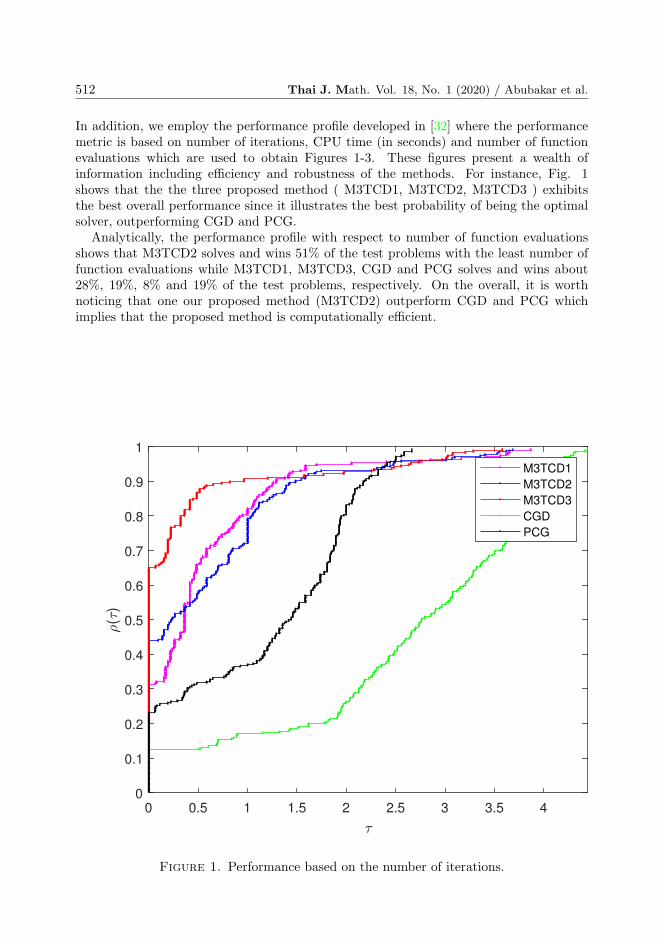
In addition, we employ the performance profile developed in [32] where the performancemetric is based on number of iterations, CPU time (in seconds) and number of functionevaluations which are used to obtain Figures 1-3. These figures present a wealth ofinformation including efficiency and robustness of the methods. For instance, Fig. 1shows that the the three proposed method ( M3TCD1, M3TCD2, M3TCD3 ) exhibitsthe best overall performance since it illustrates the best probability of being the optimalsolver, outperforming CGD and PCG.

Analytically, the performance profile with respect to number of function evaluationsshows that M3TCD2 solves and wins 51% of the test problems with the least number offunction evaluations while M3TCD1, M3TCD3, CGD and PCG solves and wins about28%, 19%, 8% and 19% of the test problems, respectively. On the overall, it is worthnoticing that one our proposed method (M3TCD2) outperform CGD and PCG whichimplies that the proposed method is computationally efficient.

0 0.5 1 1.5 2 2.5 3 3.5 40

0.1

0.2

0.3

0.4

0.5

0.6

0.7

0.8

0.9

1

()

M3TCD1

M3TCD2

M3TCD3

CGD

PCG

Figure 1. Performance based on the number of iterations.


0 0.5 1 1.5 2 2.5 3 3.5 4 4.50

0.1

0.2

0.3

0.4

0.5

0.6

0.7

0.8

0.9

1

()

M3TCD1

M3TCD2

M3TCD3

CGD

PCG

Figure 2. Performance based function evaluation.


0 0.5 1 1.5 2 2.5 3 3.5 4 4.50

0.1

0.2

0.3

0.4

0.5

0.6

0.7

0.8

0.9

1

()

M3TCD1

M3TCD2

M3TCD3

CGD

PCG

Figure 3. Performance based on CPU time.

4. Conclusions

In this article, we modified the well known conjugate descent (CD) direction and pro-posed three distinct spectral conjugate gradient algorithms for solving (1.1). The modifi-cation was achieved by adding the term −λkF (xk) to the CD direction making it three-term. Using three different approaches as in [33], we obtained three distinct definition ofλk corresponding to the three directions M3TCD1, M3TCD2 and M3TCD3 respec-tively. The proposed directions are bounded and satisfy the sufficient descent property.The convergence of the proposed algorithms was established under suitable assumptions.Finally, we give some numerical experiments to show the efficiency of the algorithmscompared with two existing algorithms namely; CGD and PCG.

Acknowledgements

This project was supported by Theoretical and Computational Science (TaCS) Cen-ter under Computational and Applied Science for Smart research Innovation Cluster(CLASSIC), Faculty of Science, KMUTT. The first author was supported by the Petchra


Pra Jom Klao Doctoral Scholarship, Academic for Ph.D. Program at KMUTT (GrantNo.26/2560).

References

[1] S.V. M. Iusem, N Alfredo, Newton-type methods with generalized distances for con-strained optimization, Optimization 41(3)(1997) 257–278.

[2] M. AT Figueiredo, R.D. Nowak, S.J. Wright, Gradient projection for sparse recon-struction: Application to compressed sensing and other inverse problems, IEEE Jour-nal of selected topics in signal processing 1(4)(2007) 586–597.

[3] T.L. Magnanti, G. Perakis, Solving variational inequality and fixed point problems byline searches and potential optimization, Mathematical programming 101(3)(2004)435–461.

[4] M. Al-Baali, Y. Narushima, H. Yabe, A family of three-term conjugate gradientmethods with sufficient descent property for unconstrained optimization, Computa-tional Optimization and Applications 60(1)(2015) 89–110.

[5] W.W. Hager H. Zhang, A survey of nonlinear conjugate gradient methods, Pacificjournal of Optimization, 2(1)(2006) 35–58.

[6] Y. Narushima, A smoothing conjugate gradient method for solving systems of non-smooth equations, Applied Mathematics and Computation, 219(16)(2013) 8646–8655.

[7] Y. Narushima, H. Yabe, J. Ford, A three-term conjugate gradient method withsufficient descent property for unconstrained optimization, SIAM Journal on Opti-mization, 21(1)(2011) 212–230.

[8] L. Zhang, W. Zhou, Spectral gradient projection method for solving nonlinear mono-tone equations, Journal of Computational and Applied Mathematics, 196(2)(2006)478–484.

[9] H. Mohammad, A.B. Abubakar, A positive spectral gradient-like method for non-linear monotone equations, Bulletin of Computational and Applied Mathematics5(1)(2017) 99–115.

[10] A.B. Abubakar P. Kumam, An improved three-term derivative-free method forsolving nonlinear equations, Computational and Applied Mathematics, 37(5)(2018)6760–6773.

[11] M.V. Solodov B.F. Svaiter, A globally convergent inexact newton method for systemsof monotone equations, In Reformulation: Nonsmooth, Piecewise Smooth, Semis-mooth and Smoothing Methods (1998) 355–369.

[12] M. Ahookhosh, K. Amini, S, Bahrami, Two derivative-free projection approachesfor systems of large-scale nonlinear monotone equations, Numerical Algorithms,64(1)(2013) 21–42.

[13] Zoltan Papp and Sanja Rapajic, Fr type methods for systems of large-scale nonlinearmonotone equations, Applied Mathematics and Computation, 269(2015) 816 – 823.

[14] D. Feng, M. Sun, X. Wang, A family of conjugate gradient methods for large-scalenonlinear equations, Journal of Inequalities and Applications, 2017 (2017) 236.

[15] A.B. Abubakar, P. Kumam, H. Mohammad, A.M. Awwal, K. Sitthithakerngkiet, Amodified fletcher–reeves conjugate gradient method for monotone nonlinear equationswith some applications, Mathematics 7(8)(2019) 745.


[16] A.B. Abubakar, P. Kumam, A.M. Awwal, A descent dai-liao projection method forconvex constrained nonlinear monotone equations with applications, Thai Journal ofMathematics 17(1)(2018).

[17] A.B. Abubakar, P. Kumam, A.M. Awwal, P. Thounthong, A modified self-adaptiveconjugate gradient method for solving convex constrained monotone nonlinear equa-tions for signal recovery problems, Mathematics 7(8)(2019) 693.

[18] A.A. Muhammed, P. Kumam, A.B. Abubakar, A. Wakili, N. Pakkaranang, A newhybrid spectral gradient projection method for monotone system of nonlinear equa-tions with convex constraints, Thai Journal of Mathematics, 16(4)(2018).

[19] A.B. Abubakar, P. Kumam, A descent dai-liao conjugate gradient method for non-linear equations, Numerical Algorithms, 81(1)(2019) 197–210.

[20] A.M. Awwal, P. Kumam, A.B. Abubakar, A modified conjugate gradient method formonotone nonlinear equations with convex constraints, Applied Numerical Mathe-matics 145(2019) 507 – 520.

[21] A.M. Awwal, P. Kumam, A.B. Abubakar, Spectral modified polak–ribiere–polyakprojection conjugate gradient method for solving monotone systems of nonlinearequations, Applied Mathematics and Computation 362(2019) 124514.

[22] A.B. Abubakar, P. Kumam, H. Mohammad, A.M. Awwal, An efficient conjugategradient method for convex constrained monotone nonlinear equations with applica-tions, Mathematics, 7(9)(2019) 767.

[23] Y. Xiao, H. Zhu, A conjugate gradient method to solve convex constrained monotoneequations with applications in compressive sensing, Journal of Mathematical Analysisand Applications, 405(1)(2013) 310–319.

[24] J.K. Liu, S.J. Li, A projection method for convex constrained monotone nonlin-ear equations with applications, Computers & Mathematics with Applications70(10)(2015) 2442–2453.

[25] W.L. Cruz, J. Martınez, M. Raydan, Spectral residual method without gradientinformation for solving large-scale nonlinear systems of equations, Mathematics ofComputation 75(255)(2006) 1429–1448.

[26] W.L. Cruz, J.M. Martınez, M. Raydan, Spectral residual method without gradientinformation for solving large-scale nonlinear systems of equations, Mathematics ofComputation 75(255)(2006) 1429–1448.

[27] W. Zhou, D. Li, Limited memory bfgs method for nonlinear monotone equations,Journal of Computational Mathematics 25(1)(2007).

[28] W.L. Cruz, A spectral algorithm for large-scale systems of nonlinear monotone equa-tions, Numerical Algorithms 76(4)(2017) 1109–1130.

[29] C. Wang, Y. Wang, and C. Xu, A projection method for a system of nonlinearmonotone equations with convex constraints, Mathematical Methods of OperationsResearch 66(1)(2007) 33–46.

[30] Y. Bing, G. Lin, An efficient implementation of merrills method for sparse or partiallyseparable systems of nonlinear equations, SIAM Journal on Optimization, 1(2)(1991)206–221.

[31] G. Yu, S. Niu, J. Ma, Multivariate spectral gradient projection method for nonlinearmonotone equations with convex constraints, Journal of Industrial and ManagementOptimization 9(1)(2013) 117–129.

[32] E.D. Dolan, J.J. More, Benchmarking optimization software with performance pro-files, Mathematical Programming 91(2)(2002) 201–213.


[33] Z. Papp, S. Rapajic, Fr type methods for systems of large-scale nonlinear monotoneequations, Applied Mathematics and Computation (2015) 269:816–823.

spectral three-term conjugate descent method for …

Documents