spectral linewidth and coherence
TRANSCRIPT

Spectral linewidth and coherence
Johanne Lein
Thesis submitted for the degree of
Master of Science
Department of Physics
Faculty of Natural Sciences
University of Oslo
2010


Abstract
Our aim has been to give a contribution to the study of the nature and wave-particleduality of light through an analysis of the concept of optical coherence. We havecarried out a numerical study of a pulse model of light, and experimentally de-termined the temporal coherence length of the spectral line of wavelength 692 nmin neon. The experimental setup proved to be less accurate than expected, but themeasurements indicate a coherence length in the order of 30 mm. The numericalsimulations suggest the possibility of using the auto-correlation function to determ-ine the temporal size of pulses of electromagnetic radiation.
iii

iv

Acknowledgments
A lady I know lives and works in a community of people with strong mental han-dicaps. Part of her work is to teach them gardening. She told me: Weeding ishard work, and even more so when you not only have to pull the weed, but alsothe person weeding. Over the past two years, I have often pictured myself as theperson being pulled, clinging to my thesis while the real work was being done bythose around me. I therefore would like to direct my thanks to...
...my supervisor, Arnt Inge Vistnes for his dedication to the work of his students.
...Borys Jagielski, PhD student and my senior in the lab by one year, both of whichmade him an infallible source of Matlab tips, oscilloscope s.o.s, and general wisdom.
...Efim Brondz, our very easy-to-ask engineer.
...Erik Alfsen, Joakim Bergli, Håkon Brox, Simen Kvaal, and Sølve Selstø for ourdiscussions.
...Håkon Bjørgen, Torbjørn Næss, and Mikkjel Thorsrud who, challenging their(strongly) theoretical disposition, helped me with lab work, pressing the buttonof the oscilloscope when time didn’t allow me to fight with the trigger, and KyrreNess Sjøbæk, for his help with the numerical part of the work.
...The students in the MEF/MENA program and on the group of theoretical phys-ics, these five years would have been much less fun if you weren’t there.
...My uncle Peter Luitjens who proofread my thesis.
...My family, for being very easy to impress, and my friends outside the departmentof physics who from time to time forced me out of my dark lab and the bubble ofMatlab simulations into the real world.
...The sisters of Abbaye de Sainte Marie de Maumont and Sta. Katarinahjemmetfor all their help, ranging from moral support and prayers to supplying LATEXcode.
v

vi

Contents
Acknowledgements v
Introduction 1
1 Models of light 5
1.1 Ray optics . . . . . . . . . . . . . . . . . . . . . . . . . . . . . . . . 61.2 Wave optics and the beam model of light . . . . . . . . . . . . . . . 11
2 Coherence 19
2.1 Interference . . . . . . . . . . . . . . . . . . . . . . . . . . . . . . . 192.2 Coherence . . . . . . . . . . . . . . . . . . . . . . . . . . . . . . . . 21
2.2.1 The n’th order correlation function . . . . . . . . . . . . . . 222.2.2 Classical theoretical value of coherence length . . . . . . . . 25
2.3 Coherence as predictability . . . . . . . . . . . . . . . . . . . . . . 31
3 Simulations 33
3.1 Generation of signals . . . . . . . . . . . . . . . . . . . . . . . . . . 343.2 Matlab code for analysis . . . . . . . . . . . . . . . . . . . . . . . . 35
3.2.1 The auto-correlation function . . . . . . . . . . . . . . . . . 353.2.2 Simulation of a Michelson’s interferometer . . . . . . . . . . 363.2.3 Power spectral density . . . . . . . . . . . . . . . . . . . . . 36
3.3 The Wiener-Khinchine theorem . . . . . . . . . . . . . . . . . . . . 363.4 Visibility and the auto-correlation function . . . . . . . . . . . . . . 373.5 Wave packets, photons and coherence length . . . . . . . . . . . . . 40
3.5.1 Does the coherence length correspond to the photon size? . 40
4 Components of the experimental setup 53
4.1 Spectral lamps . . . . . . . . . . . . . . . . . . . . . . . . . . . . . 534.1.1 Broadening mechanisms . . . . . . . . . . . . . . . . . . . . 55
4.2 Fabry-Perot interferometer and interference filter . . . . . . . . . . 614.3 Optic fibers . . . . . . . . . . . . . . . . . . . . . . . . . . . . . . . 63
5 Experimental setup and methods 73
5.1 Measuring the spectral line widths of light sources . . . . . . . . . 735.2 Measuring coherence length of light sources . . . . . . . . . . . . . 79
5.2.1 General outline of the experiment . . . . . . . . . . . . . . . 80
vii

viii CONTENTS
5.2.2 Collimating light into an optic fiber . . . . . . . . . . . . . . 805.2.3 Achieving high visibility . . . . . . . . . . . . . . . . . . . . 815.2.4 Positioning of mirrors using white light interference . . . . . 85
5.3 Changing path length . . . . . . . . . . . . . . . . . . . . . . . . . 875.3.1 Platform with µm-screw . . . . . . . . . . . . . . . . . . . . 875.3.2 Piezo-element . . . . . . . . . . . . . . . . . . . . . . . . . . 875.3.3 Step-motor . . . . . . . . . . . . . . . . . . . . . . . . . . . 88
5.4 Detectors . . . . . . . . . . . . . . . . . . . . . . . . . . . . . . . . 935.4.1 USBeamPro . . . . . . . . . . . . . . . . . . . . . . . . . . . 935.4.2 Silicon photodetector (SPD) and power meter . . . . . . . . 945.4.3 Single photon counting module (SPCM) . . . . . . . . . . . 965.4.4 LeCroy digital oscilloscope . . . . . . . . . . . . . . . . . . . 975.4.5 Time-digitizer . . . . . . . . . . . . . . . . . . . . . . . . . . 99
6 Experimental results for Ne692 101
6.1 Measurements . . . . . . . . . . . . . . . . . . . . . . . . . . . . . . 1016.2 Discarding data . . . . . . . . . . . . . . . . . . . . . . . . . . . . . 102
6.2.1 Discarding the data for ∆l = 30 mm . . . . . . . . . . . . . 1026.2.2 Discarding of data due to hysteresis of piezo-element . . . . 103
6.3 Finding the visibility of the spectral lamps . . . . . . . . . . . . . . 1046.4 Pulse number-density . . . . . . . . . . . . . . . . . . . . . . . . . . 107
7 Summary and outlook 109
A Fourier transforms 113
A.1 General introduction . . . . . . . . . . . . . . . . . . . . . . . . . . 113A.2 Fourier transform of a Gaussian function . . . . . . . . . . . . . . . 115
B Data 119
B.1 Data . . . . . . . . . . . . . . . . . . . . . . . . . . . . . . . . . . . 119B.2 Code for finding least square fit of sine to data . . . . . . . . . . . 123
C Program used in simulations 125
C.1 Main program . . . . . . . . . . . . . . . . . . . . . . . . . . . . . . 126C.2 Plotting the original signal and its Fourier transform . . . . . . . . 127C.3 Plotting the auto-correlation function . . . . . . . . . . . . . . . . . 129C.4 Simulating a Michelson’s interferometer . . . . . . . . . . . . . . . 131C.5 Power spectral density . . . . . . . . . . . . . . . . . . . . . . . . . 133

Introduction
“We are convinced that our present problems, our methods, our sci-entific concepts are, at least partly, the results of a scientific traditionwhich accompanies or leads the way of science through the centuries.It is therefore natural to ask to what extent our present work is de-termined or influenced by tradition. Are the problems in which we areengaged freely chosen according to our interest or inclination, or arethey given to us by an historical process? To what extent can we selectour scientific methods according to the purpose, to what extent do weagain follow a given tradition? And finally how free are we in choosingthe concepts for formulating our questions? Any scientific work canonly be defined by formulating the questions which we want to answer.But in order to formulate the questions we need concepts by which wehope to get hold of the phenomena. These concepts usually are takenfrom the past history of science; they suggest already a possible pictureof the phenomena. But if we are going to enter into a new realm ofphenomena, these concepts may act as a collection of prejudices, whichhamper progress rather than foster it” (Werner Heisenberg in [21]).
In every subject there comes a point when one has to accept some facts. To be ableto build one needs to be on solid ground. If not, one will find oneself flounderingawkwardly about in a confusing vacuum. Science will never advance if every sci-entist were to do everything from scratch. If we know more than our predecessors,it is because of what they gave us. Every physicist should recognize themselves inwhat sir Isaac Newton famously wrote: “If I have seen further, it is by standingon the shoulders of giants” [31].
However, as Heisenberg argues in the opening quote, the scientific tradition is al-ways in danger of being a collection of prejudices. Every once in a while, oneneeds to critically examine the giants. They, also, need our support and approvalto remain standing. The work that is being performed at Oslo Quantum-opticLaboratory has the expressed goal of examining one of these giants, namely thatof the duality of the nature of light.
As the title suggests, the work that has been done has centered around the conceptof coherence time and length. A passable definition of the term coherence time is
1

2 CONTENTS
the time τ one may predict the state of the system if one knows its current state.Coherence length of light is the length covered by the light in that time: lcoh = cτ ,where c is the speed of light. The above definition will be closer analysed andspecified in the course of the work. Our aim has been to obtain a greater under-standing of the concept of optical coherence through experimental measurementson light emitted from gasses consisting of a single chemical element.
While working on the thesis, the author has collaborated with Borys Jagielski andArnt Inge Vistnes on a numerical analysis of various methods of determining tem-poral coherence length for different models of light. It should be mentioned thatmuch of what is being discussed in the thesis is, directly or indirectly, a fruit ofthat collaboration.
Some authors have indirectly suggested that the coherence time of light is a meas-ure of the temporal size of a photon [2], [25]. As we will see, this is plausible if oneexamines a single photon depicted as a wave-packet of electromagnetic radiation.It may, however, become problematic if the signal to be examined is a collection ofmany such wave-packets. It has been said about the electron that “We experienceit as a causal tie or link between two events, its "birth" in the electron source andits death (or transmutation) in the interaction with the detector” [19]. It seemsthat this could equally well have been uttered about particles of light, but, in thatcase, must that link always be a one-to-one relation between its emission from thesource and its absorption in our detectors?
The somewhat sloppy definition of coherence time as being linked to the predict-ability of a system also seems to suggest a picture of coherence length of being dueto more or less random fluctuations in the system. Is it possible that the coherencetime and length of a light source is an indication of the average time between thefluctuations in the source? During our work, we will keep this picture in mind.
We begin in chapter one by introducing the model of light that will serve to giveus the mental pictures needed in the continuation. In chapter two, we will brieflydescribe the phenomenon of interference, before introducing the main topic of thethesis, coherence of light. The predictions made in this chapter will form the basisof numerical simulations, the results of which will be presented in chapter three.We will also discuss the concept of the photon, and show how its size may be un-derstood in relation to the coherence length found in the simulations. In chapterfour and five, the experimental setup and methods are described in some detail.The experimental results will be presented and discussed in chapter six, and wewill round off in chapter seven with a summary and some concluding remarks. Inaddition, a brief, conceptional review of Fourier transforms, the experimental data,and the program used in simulations have been included in appendices.
It should be mentioned that much time has been spent doing the seemingly trivialwork of building up and testing the experimental setup. In quantum optics, doing

CONTENTS 3
an experiment in general means spending hours of choosing the right pieces ofequipment, aligning and adjusting, and re-aligning and re-adjusting them. Theauthor is only the second student to obtain a master’s degree at the laboratory,and the first whose work has been completely centered around experiment1. Partof the goal has therefore been to take part in choosing and purchasing experimentalequipment, to gain competence and learn about its behaviour in practical applic-ation, to test and develop methods for our specific use, and to describe it all toallow future students to avoid the mistakes, improve that which has potential forimprovement, and, maybe, repeat that which was successful.
The theory that is presented has also been chosen with an experimental ratherthan theoretical goal in mind. The author has tried to give a simple and pragmaticpresentation of background information and concepts, while keeping the question“why and how does it work?” in mind. As a result, a person more theoreticallyminded will possibly find that some details are excessively elaborated, while otherinteresting relations are omitted. Hopefully, future students may also here benefitfrom the choices made.
Let us in closing include a few words on the notation used. Some figures are madeup of several sub-figures. These will, starting from the top left, be denoted (a),(b), and so on. Since we are only working with relative quantities, most constantsof normalisation have been excluded. In particular, the intensity is said to be theabsolute square of the electric field, I = |E|2, omitting the constant ǫ0c/2. Also,the symbols λ and c are taken to be the wavelength and speed of the light in amedium. To denote the wavelength and speed of light in vacuum, we will writeλvac and cvac. As described in appendix A, if F and G are Fourier pairs, we willwrite F ⇀↽ G.
1The first student was Borys Jagielski, whose thesis also included experimental work. Themain focus, however, was theoretical.

4 CONTENTS

Chapter 1
Models of light
Often in the natural sciences, many models that describe the same phenomenonexist side by side. The different models may emphasize different aspects of thephysical reality that they aim to describe. Although a model rarely or never canclaim to capture the whole truth of the phenomenon in question, several modelstaken together may offer a more complete picture.
In the physics of optics, various models often fit into one of two main categories:The particle and the wave description of light. In the particle description lightis perceived as a collection of indivisible quanta. At the present moment perceiv-ing light as particles or quanta seems to offer the best explanation of the resultsof coincidence experiment, where light is sent through a beam splitter and intodetectors on the two outgoing sides. If the intensity of the light is very low, thedetectors do not respond at the same time, and this is interpreted as a proof thatlight is indeed made up of indivisible entities [16].
The wave description builds on Maxwell’s equations, and in it, light is perceivedas continuous, propagating electromagnetic fields. As we will see, the model al-lows for describing interference and diffraction phenomena of light with a rathersimple mathematical formalism, and for intuitive conceptional analogies to otherwave-phenomena in nature.
It is difficult to conceive a phenomenon both as a continuous field and as indivisibleparticles. Efforts have been made to force light to reveal the interference patternwithout actually interacting with it, to be able to experimentally see examples ofwave and particle behaviour at the same time [2], but there is not full consensusof the validity of the conclusions from such experiments [14], [46].
A thorough discussion of historical and experimental aspects of the wave-particleduality of light is given in [22].
In section 1.2, we will introduce the beam model that will serve as our referencein the continuation. As an hors d’oeuvre, we have included a description of a
5
6 CHAPTER 1. MODELS OF LIGHT
geometrical ray model. This ray model will not, or very little, be referred to in thecontinuation, but has been included since it with some simple geometrical argu-ments allows us to find a formula for the propagation of light through an opticalsystem that, once derived in the ray model, may easily be transferred to and jus-tified in the beam model.We have not meant to give an exhaustive description ofeither of the two model, but a pragmatic introduction of concepts that will becomeuseful in describing the experimental work.
1.1 Ray optics
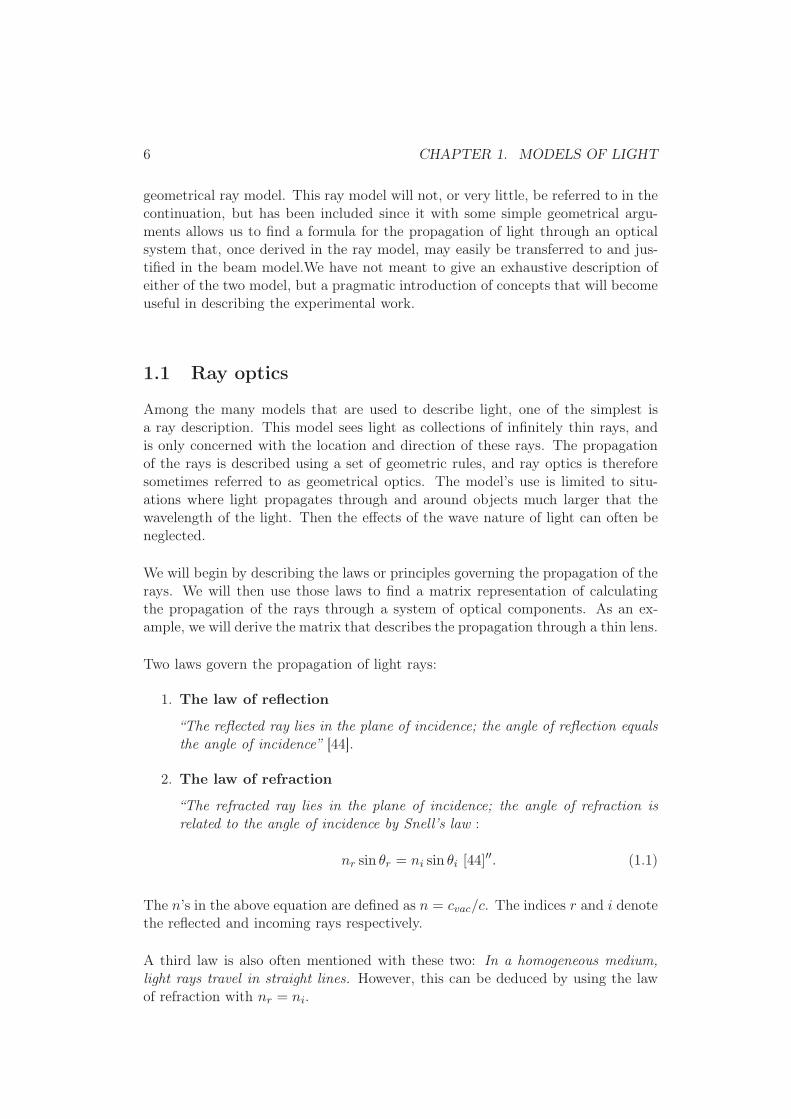
Among the many models that are used to describe light, one of the simplest isa ray description. This model sees light as collections of infinitely thin rays, andis only concerned with the location and direction of these rays. The propagationof the rays is described using a set of geometric rules, and ray optics is thereforesometimes referred to as geometrical optics. The model’s use is limited to situ-ations where light propagates through and around objects much larger that thewavelength of the light. Then the effects of the wave nature of light can often beneglected.
We will begin by describing the laws or principles governing the propagation of therays. We will then use those laws to find a matrix representation of calculatingthe propagation of the rays through a system of optical components. As an ex-ample, we will derive the matrix that describes the propagation through a thin lens.
Two laws govern the propagation of light rays:
1. The law of reflection
“The reflected ray lies in the plane of incidence; the angle of reflection equalsthe angle of incidence” [44].
2. The law of refraction
“The refracted ray lies in the plane of incidence; the angle of refraction isrelated to the angle of incidence by Snell’s law :
nr sin θr = ni sin θi [44]′′. (1.1)
The n’s in the above equation are defined as n = cvac/c. The indices r and i denotethe reflected and incoming rays respectively.
A third law is also often mentioned with these two: In a homogeneous medium,light rays travel in straight lines. However, this can be deduced by using the lawof refraction with nr = ni.

1.1. RAY OPTICS 7
Figure 1.1: Light ray propagating a distance d through homogeneous medium
ABCD-matrix in ray optics
As mentioned above, ray optics is only concerned with the position and directionof a ray of light. If we assume that the ray is propagating in the (x, y)-plane, theray will be unambigously determined if we know its y-position for some x, and theangle θ it makes with the x-axis. Examining figure 1.1, one finds that for a raypropagating a distance whose x-component is d, in a homogeneous medium, onefinds that y2 and θ2 at the point x2 are
y2 = 1 × y1 + d× tan θ1
tan θ2 = 0 × y1 + 1 × tan θ1,
where y1, θ1 are the y-position and angle with the x−axis when x = x1.
In the paraxial approximation, with all θi being small so that tan θi ≈ sin θi ≈ θi,this can be written:
(
y2
θ2
)
=
(
1 d0 1
)(
y1
θ1
)
.
In general, any optical system can in the paraxial approximation be written in theform
(
y2
θ2
)
= M
(
y1
θ1
)
, with M =
(
A BC D
)
.
If the optical system consists of i components, each with ABCD-matrix
mi =
(
ai bici di
)
,
the final matrix M is just the product of the separate matrices. The outcomeof the system of optical components is uniquely determined by the final matrix

8 CHAPTER 1. MODELS OF LIGHT
M =∏
i
mi. Two systems of different optical components with matrices mi that
multiply to the same matrix M will have the same effect on the propagation ofthe light, as illustradet with the “black box” in figure 1.2. When finding the totalmatrix M of a system of optical components, the far left matrix will correspondto the last optical component, since it will be the last matrix to operate on the
vector
(
yθ
)
.
Figure 1.2: Propagation of a light ray through some optical system is uniquely determined
by the ABCD-matrix of the total system. The matrix of the system is the product of the
matrices of its components.
ABCD-matrix for propagation through a thin lens
To make even clearer the concept of the ABCD-method, and since it will be rel-evant in the experimental setup, let us find the matrix for propagation of a raythrough a thin lens.
When the ray crosses a boundary of refraction, the y-parameter will, because ofcontinuity, remain the same, y = y2 = y1, where y1 and y2 are the distances to theaxis of propagation as the ray hits and leaves the boundary respectively.
From figure 1.3, Snell’s law for refraction through a curved surface gives
n1 sin (α+ θ1) = n2 sin (α− θ2).
Assuming that α, θ1 and θ2 are small1 this is
n1(α+ θ1) = n2(α− θ2)
⇒ θ2 =n2α− n1(α+ θ1)
n2=n2 − n1
n2Ry1 −
n1
n2θ1
1the θ’s are small by the assumption that we work in the paraxial approximation, the α issmall since we are looking at a thin lens. Using a thin lens, the y-position of the ray will alwaysbe much smaller than the radius of curvature of the lens, and α can therefore be assumed to besmall.

1.1. RAY OPTICS 9
Figure 1.3: If the lens is thin, the difference in position, ∆y, can be neglected, and the
matrix for a ray through the lens equals the product of the matrices of two curved surfaces
where in the last line we have used the identity
α ≈ sinα = y/R,
which can be verified by studying figure 1.3. Thus, the matrix of refraction througha curved surface is:
(
1 0n2−n1n2R −n1
n2
)
. (1.2)
Now, the matrix for diffraction through a lens is the product of three matrices:That of propagation through a homogeneous media wedged between the matricesof refraction through two curved surfaces2. Since we are assuming the lens to bethin, the matrix of propagation will be almost equal to the identity matrix, so thetotal matrix of the lens will be the product of the matrices of two surfaces withradii R1 and R2:
(
1 0n1−n2n1R1
−n2n1
)(
1 0n2−n1n2R2
−n1n2
)
=
(
1 0n1−n2
n1( 1
R1+ 1
R2) 1
)
≡(
1 0− 1
f 1
)
. (1.3)
The f in the above equation is called the focal length of the lens and is perhapsthe most important parameter of the lens.
2Note that in the second surface (the leftmost matrix) n2 will be the refractive index at theincoming surface, and n1 at the outgoing, opposite to that of equation (1.2). Note also thatthe definition of the sing of the radius of a boundry, and therefore the C-parameter of the thirdmatrix in (1.3) may look slightly different in different texts.
10 CHAPTER 1. MODELS OF LIGHT
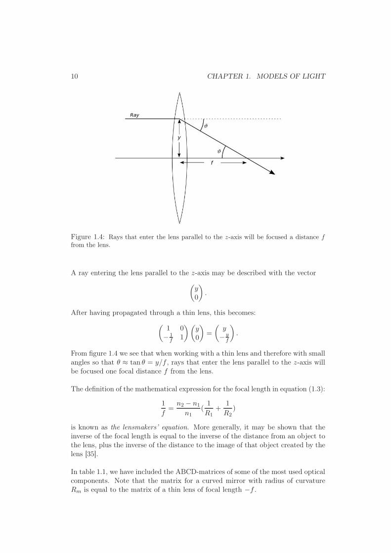
Figure 1.4: Rays that enter the lens parallel to the z-axis will be focused a distance ffrom the lens.
A ray entering the lens parallel to the z-axis may be described with the vector
(
y0
)
.
After having propagated through a thin lens, this becomes:
(
1 0− 1
f 1
)(
y0
)
=
(
y− y
f
)
.
From figure 1.4 we see that when working with a thin lens and therefore with smallangles so that θ ≈ tan θ = y/f , rays that enter the lens parallel to the z-axis willbe focused one focal distance f from the lens.
The definition of the mathematical expression for the focal length in equation (1.3):
1
f=n2 − n1
n1(
1
R1+
1
R2)
is known as the lensmakers’ equation. More generally, it may be shown that theinverse of the focal length is equal to the inverse of the distance from an object tothe lens, plus the inverse of the distance to the image of that object created by thelens [35].
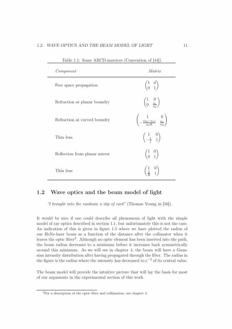
In table 1.1, we have included the ABCD-matrices of some of the most used opticalcomponents. Note that the matrix for a curved mirror with radius of curvatureRm is equal to the matrix of a thin lens of focal length −f .
1.2. WAVE OPTICS AND THE BEAM MODEL OF LIGHT 11
Table 1.1: Some ABCD-matrices (Convention of [44]).
Component Matrix
Free space propagation
(
1 d0 1
)
Refraction at planar boundry
(
1 00 n1
n2
)
Refraction at curved boundry
(
1 0
− (n2−n1)n2R
n1n2
)
Thin lens
(
1 0− 1
f 1
)
Reflection from planar mirror
(
1 00 1
)
Thin lens
(
1 02R 1
)
1.2 Wave optics and the beam model of light
”I brought into the sunbeam a slip of card” (Thomas Young in [56]).
It would be nice if one could describe all phenomena of light with the simplemodel of ray optics described in section 1.1, but unfortunately this is not the case.An indication of this is given in figure 1.5 where we have plotted the radius ofour HeNe-laser beam as a function of the distance after the collimator when itleaves the optic fiber3. Although no optic element has been inserted into the path,the beam radius decreases to a minimum before it increases back symmetricallyaround this minimum. As we will see in chapter 4, the beam will have a Gaus-sian intensity distribution after having propagated through the fiber. The radius inthe figure is the radius where the intensity has decreased to e−2 of its central value.
The beam model will provide the intuitive picture that will lay the basis for mostof our arguments in the experimental section of this work.
3For a description of the optic fiber and collimation, see chapter 4.

12 CHAPTER 1. MODELS OF LIGHT
0 200 400 600 800 1000100
200
300
400
500
600
700
Distance from fiber/mm
Bea
m r
adiu
s/µm
Figure 1.5: The profile of the laser beam after it leaves the collimator on the outgoing
side of the optic fiber.
Young’s double slit experiment
One of the first demonstrations of the wave nature of light was the famous “doubleslit experiment” performed by the British physicist Thomas Young at the begin-ning of the 19th century. When bringing a thin piece of cardboard into a beam ofsunlight and examining the pattern of the light falling on a screen behind the card,he found that the one piece of card produced a pattern of several dark and brightfringes. The idea of light having wave-like properties was not new. Refractionphenomena of light had been observed by physicists before Young, and some hadconcluded that light possessed wavelike, or oscillating, properties. It is nonthelessthe article in which Young presented his ideas to the Physical Society of Londonthat has come to be considered the modern revival of the wave theory of light [22].
Young himself never uses the word “waves” in his article, but he argues that onemay infer from his experiments that light
“...is possessed of opposite qualities, capable of neutralising or destroy-ing each other, and of extinguishing the light, where they happen to beunited; that these qualities succeed each other alternately (...) at dis-tances which are constant for the same light passing through the samemedium” [56].
He equally urges “those who are attached to the Newtonian theory of light”, that is,those who believe in a corpuscular theory of light [32], to make an effort to explainhis results using their own theory or
“...if they fail in the attempt, to refrain at least from idle declamationagainst a system which is founded on the accuracy of its application toall these facts, and to a thousand others of a similar nature” [56].4
4Though of no relevance to the theme of this thesis, let us, purely for the sake of its beauty,offer one more example of the poetic langage of Young’s article, in which he discusses the pos-

1.2. WAVE OPTICS AND THE BEAM MODEL OF LIGHT 13
The beam model from Maxwell’s equations
Standard electromagnetism tells us that light is a type of electromagnetic phenom-ena. Maxwell’s equations state that if E denotes the electric and H the magneticfield, one has:
∇× E = −µ∂H
∂t (1.4a)
∇× H = ǫ∂E
∂t (1.4b)
∇ · E = 0 (1.4c)
∇ ·H = 0 (1.4d)
given that the media is linear5, isotropic6, and dielectric7 without currents or freecharges. Taking the curl of equation (1.4a) gives
∇× (∇× E) = −µ ∂∂t
∇× H
and using the identity
∇× (∇× v) = ∇(∇ · v) −∇2v
together with (1.4c) on the left hand side, and (1.4b) on the right hand side gives
∇2E = ǫµ
∂2E
∂t2.
Equivalently, one can find that
∇2H = ǫµ
∂2H
∂t2.
These equations must be satisfied for all the components of the electric and mag-netic field separately. To simplify the notation we write
∇2u =1
c2∂2u
∂t2. (1.5)
where u = u(r, t) is any of the six components of the electric and magnetic fields,and r = (x, y, z) is the position vector. Equation (1.5) is a wave-equation, and
sibility of light moving through an ether: “I am disposed to believe, that the luminiferous etherpervades the substance of all material bodies with little or no resistance, as freely perhaps as thewind passes through a grove of trees” [56].
5Linear: Having the property that the polarisation-vector is parallel and proportional to theelectric field [51].
6Isotropic: “Denoting a medium whose physical properties are independent of direction” [12].7Dielectric: “A nonconductor (...) in which an applied electric field causes a displacement
of charge but not a flow of charge” [12].

14 CHAPTER 1. MODELS OF LIGHT
the electromagnetic field may therefore be interpreted as a phenomenon exhibitingwave-like properties.
It will prove useful to expand the wave function u with an imaginary part. We canthen write this new complex wave function as
U(r, t) = U(r)ei2πνt = a(r)eiφ(r)ei2πνt (1.6)
and define our real wave function to be u = Re{U(r, t)}. In equation (1.6), φ issome parameter that describes the phase of the beam at a certain point r. Thewave fronts of the beam are surfaces of constant phase φ, that move with speedc ≡ 1/
√ǫµ. All information about the electromagnetic wave and its propagation
is now contained in U(r, t).
The time-independent part, U(r) = a(r)eiφ(r) is commonly referred to as the com-plex amplitude of the wave. In the following, when we write only U , we will takeit to mean U(r). The complex wave function has to obey the same wave-equationas its real part. When putting the expression for U(r, t) into equation (1.5), theexponential containing all the time-dependence is kept constant and cancels out,and we are left with
∇2U + k2U = 0, (1.7)
where we have used the definition k = 2πνc .
We will in the following see how equation (1.7) brings fourth the Gaussian beamas a possible allowed solution for propagating light. In chapter 4 we will showhow to experimentally shape a beamfront to become Gaussian, and see why thisis essential in carrying out experiments in optics.
The paraxial approximation
It is possible to show more subtly the connection between the models of wavesand rays, but suffice it here to simply state that the rays of ray optics are parallelto the normals of the wave fronts of wave optics. As a consequence of this, themathematics of wave optics may be carried out in the paraxial approximation iftheir normals are paraxial rays, that is, if the wavefront bends only slightly.
A wave whose wavefront does not bend at all is called a plane wave. If it propagatesin the z-direction its complex amplitude can be written out
U(r) = Ae−ikz,
where A is a constant.
To allow for the wavefront to bend, we let A become a function of r, and write
U(r) = A(r)e−ikz .

1.2. WAVE OPTICS AND THE BEAM MODEL OF LIGHT 15
Putting this into equation (1.7), we are left with an equation for A(r):
∇2TA+
∂2A
∂z2− i2k
∂A
∂z= 0. (1.8)
In the above equation, ∇2T = ∂2
∂x2 + ∂2
∂x2 is the transverse Laplacian operator.
For the wavefront to be and remain in the paraxial approximation, the varianceof A and its derivative must be very small within distances in the order of awavelength [44]. We then have
δ
(
∂A
∂z
)
=∂2A
∂z2δz =
∂2A
∂z2λ <<
∂A
∂z.
Since λ = 2π/k and the factor of π is of the order of unity, the term with thedouble derivative in z in equation (1.8) may be neglected, and we are left with thesimpler equation
∇2TA− i2k
∂A
∂z= 0. (1.9)
The solutions to equation (1.9) define the set of possible waves that propagate inthe z-direction and obey the paraxial aproximation.
The Gaussian beam
Although simpler solutions to equation (1.9) exist, let us jump directly to the onethat will be relevant in the continouation of the thesis: The Gaussian beam.
A Gaussian beam may be described by [44]
A(r) =z0√I0
q(z)exp
{
−ik ρ2
2q(z)
}
, ρ = x2 + y2. (1.10)
In equation (1.10), q(z) is called the q−parameter of the beam, and is equal toz plus a constant imaginary term, q(z) = z + iz0. The quantity z0
√I0 is for the
time being just an arbitrary constant. Its somewhat peculiar appearance will proveuseful in a moment.
To show the physical meaning of the q-parameter, let us look at its inverse:
1
q=
1
z + iz0=
z
z2 + z20
− iz0
z2 + z20
≡ 1
R− i
λ
πW 2, (1.11)
where we have defined
R = R(z) ≡ z[
1 +(
z0z
)2]
W = W (z) ≡W0
√
z2 + z20
z20
, W0 ≡√
λz0π.
(1.12)

16 CHAPTER 1. MODELS OF LIGHT
Using the expressions for W and R with equation (1.10), the complex envelopemay be written out
U(r) = −i√
I0W0
W (z)exp
{
− ρ2
W 2(z)
}
exp
{
−ikz − ikρ2
2R(z)− i tan
(z0z
)
}
.
(1.13)The intensity of a beam is the square of its complex envelope [44]. In our case thisis:
I(r) = I(ρ, z) = |U(r)|2 = |A(r)|2
=I0z
20
|q(z)|2 exp
{ −kρ2λ
πW 2(z)
}
= I0
[
W0
W (z)
]2
exp
{
2ρ2
W 2(z)
}
.
(1.14)
As seen from the last part of the equation, the beam is a Gaussian function of theradial distance from the beam axis. On the beam axis, where ρ = 0, the intensityis equal to
I(0, z) = I0
[
W0
W (z)
]2
.
From equation (1.12), W (z = 0) = W0 so that
I0 = I(ρ = 0, z = 0).
The parameters W and R defined in equation (1.12) are called the waist andradius of curvature of the beam. We will now show the physical meaning of thetwo parameters.
Beam width
The ratio of the total energy of the beam within a circle of radius W (z) is
E
Etotal=
∫W (z)0 I(ρ, z)2πρ dρ∫∞0 I(ρ, z)2πρ dρ
= 1 − e−2 ≈ 0.86.
Since a high fraction of the energy is contained within a circle of radius W (z), andsince this fraction is independent of z, W (z) is called the beam width, and is oftengiven as one of the parameters needed to completely describe the propagation ofthe beam. The smallest beam width is W0 = W (z = 0), and the z = 0-plane iscalled the beam waist.
Radius of curvature
To justify giving the name radius of curvature to the quantity R let us first lookat the radius of curvature of a spherical wavefront. Spherical waves have complexamplitude U(r) = Ae−ikr, every point on the wavefront has the same radius of

1.2. WAVE OPTICS AND THE BEAM MODEL OF LIGHT 17
0 5 10 15 20 250
10
20
30
40
z / mm
phas
e
without tan−1(z/z0)
with tan−1(z/z0)
Figure 1.6: Equation 1.16 with and withouth the tan−1 (z/z0)-term. In the graphs, ρ = 10 mm,W0 = 1 mm and k = 1 mm−1. In visible light, k would be many orders of magnitude larger, andthe effect of the tan−1 (z/z0)-term would not be visible in the graph.
curvature r. Remembering that the wavefronts were defined as surfaces of constantphase, we may write
constant = kr = k√
ρ2 + z2 = kz
√
ρ2
z2+ 1 ≈ kz
(
1 +ρ2
2z2
)
≈ kz +kρ2
2r, (1.15)
where the last two steps are only valid in the paraxial approximation whereρ << |z| ≈ r.
The phase of a Gaussian wave was written out in equation (1.13). Setting thisphase to be constant, we find that for Gaussian wavefronts, it holds that
kz +kρ2
2R+ tan
(z0z
)
= constant, R = z[
1 +(
z0z
)2]
. (1.16)
If we make a plot as in figure 1.6 of the left hand side of equation (1.16) withand without the tan z0/z, we see that this term may be neglected. Without thisterm, equation (1.15) and equation (1.16) are identical with the R defined inequation (1.12) indeed playing the role of radius of curvature. As we will seein chapter 5, for measuerments of coherence length to be possible, the wavefrontsof two beams must be completely overlapping, that is, both the beam waist andradius of curvature must be similar for the overlapping beams.
ABCD-matrix in beam optics
At a first glance, it may not seem obvious that the ABCD-parameters from rayoptics can be used with a model of a propagating and developing beam. However,using the fact that the rays of ray optics are parallel to the wavefront normals, wewill see that this is indeed the case. Though qualitatively different from the matrixrepresentation of the ray model, the ABCD-equation of the beam optics will have

18 CHAPTER 1. MODELS OF LIGHT
Figure 1.7: The rays are normal to the wavefront normals. Accordingly, to work in the
paraxial approximation in the beam model means that the wavefront bends little enough
for its normals to be paraxial rays.
an appearance very similar to what we previously saw.
Recall that in the representation of paraxial rays,
y/R = sin θ ≈ θ. (1.17)
Now, let R be the radius of curvature of the beam itself (and not of a lens). Fromfigure 1.7 we see that the relation (1.17) still holds. Since the rays we had earliercorrespond to the wavefront normals, we can use the same set of equations asbefore, and we get
y2 = Ay1 +Bθ1
θ2 = Cy1 +Dθ1.
Dividing the former by the latter and using equation (1.17), one finds directly [35]
R2 =AR1 +B
CR1 +D.
It has been shown ([10], [54]) that this can be generalized to
q2 =Aq1 +B
Cq1 +D,
q being the q-parameter of the beam, whose relation to R is defined by equa-tion (1.11).

Chapter 2
Coherence
The title of this work is Spectral linewidth and coherence. Coherence in light isclosely tied with interference, a physical phenomenon found in many situationsthat involve wavelike behaviour. We will therefore begin with a short discussionof interference before moving on to defining coherence, and to define and calculatesome quantities that will help us measure the coherence of a signal.
2.1 Interference
Imagine throwing a pebble into a lake and watching the waves spread in circlesfrom where it hits the water. If you trow several pebbles into the water, they willstart out in the same way: Several circular wavefronts spreading from each pointwhere a pebble hit. After a while, when the circles have grown large enough, theybegin to mix. The resultant wave depends on the amplitude and relative phaseof the wavefronts of each of the partial waves, and the result is an interferencepattern with very many more speckles and nuances than of the original circularpattern.
Interference patterns in water is an idea intuitively easy to accept. If two wavetops of equal amplitude meet, it is only natural that the new wave has an amp-litude larger than each of the two partial waves. If a wave top meets a trough,the result would be no wave at all - at least if the partial waves were identical andconducted in a way so that a wave top always would hit a trough and vice-versa.Doing a similar experiment with light is perhaps more astonishing. In chapter 1we saw that light may be described as electromagnetic waves. In daily life, thewave-nature of light for the most part remains hidden. Even our best detectorsdo not have the temporal resolution to be able to resolve field oscillations in theorder of 1014 Hz; what they actually measure is the time average of the intensity,proportional to the square of the electric field, taken over a time window muchlarger than a period of oscillation of the light. With the help of an interferometer,light waves may be brought together and mixed in a way that lets us examine therelative phase of their electric field.
19

20 CHAPTER 2. COHERENCE
Figure 2.1: The total electric field (in black) is the sum of the electric fields of the two partialwaves. If the electric field is completely in phase, constructive interference will occur (a). If thereis a slight phase difference between the two waves, the difference of value between the maximaand the minima will be smaller, as in (b). If the difference in the two paths, ∆l, is an odd integerof half of the wavelength, the interference will be destructive (c).
0 0.5 1 1.5 2 2.5 30
0.2
0.4
0.6
0.8
1
∆l / λ
Rel
ativ
e in
tens
ity
Figure 2.2: The intensity is proportional to the square of the electric field, and changing thepath difference ∆l therefore makes the intensity oscillate.
An interferometer is an optical device that splits a beam into two and lets thetwo parts follow different paths before recombining them. The recombination ofthe two partial beams follow the principle of superposition. If the two paths areequal, the beams will recombine to form the original beam1 as in the first graphin figure 2.1. If, however, one of the partial beams has followed a path whosedistance differs with an amount ∆l with respect to the path of the other, themeasured intensity may be significantly different from what it would have been ifno interference had taken place. The second and third graphs in figure 2.1 showthe total wave created from superposing waves that have a slight phase difference,and that are completely out of phase. The intensity as function of phase differencewill oscillate as shown in figure 2.1.
To be able to measure the quality of an interference pattern, we define the quantityvisibility:
V =Imax − Imin
Imax + Imin, (2.1)
where Imax is the intensity maximum closest to I(∆l) and Imin is the intensity ofthe following minimum. It then follows that a visibility of 1 means that the wave-
1Or rather, they will recombine to form two beams, each with intensity half of the original

2.2. COHERENCE 21
fronts are perfectly overlapping, so that destructive interference brings Imin to zero.
As we will see in chapter 4, no physical light source emits purely monochromaticlight. In addition, there will always be random fluctuations that over time canchange a beam significantly. A beam with a visibility of nearly unity when ∆l inthe order of 1 mm may have been subject to many fluctuations, and therefore notshow any sign of an interference pattern when ∆l becomes close to, say, a meter.This brings us to the main topic of this chapter: Coherence.
2.2 Coherence
In the introduction we defined coherence as the time τ one may predict the state ofthe system if one knows its current state, though we admitted that this definitionwas only passable, and promised to make it more precise.
In the following, we will sometimes write intensities and electric fields as functionsof time, sometimes as functions of frequency. This has been done to make themathematics as intuitive as possible. It is implied that when we use quantitiesas functions of time, we mean the instantaneous intensity and electric field, andthat when we are working with frequency-dependent quantities, the quantity inquestion is a time-average.
Figure 2.3: The double slit experiment (Figure from [28], slightly modified)
.
22 CHAPTER 2. COHERENCE
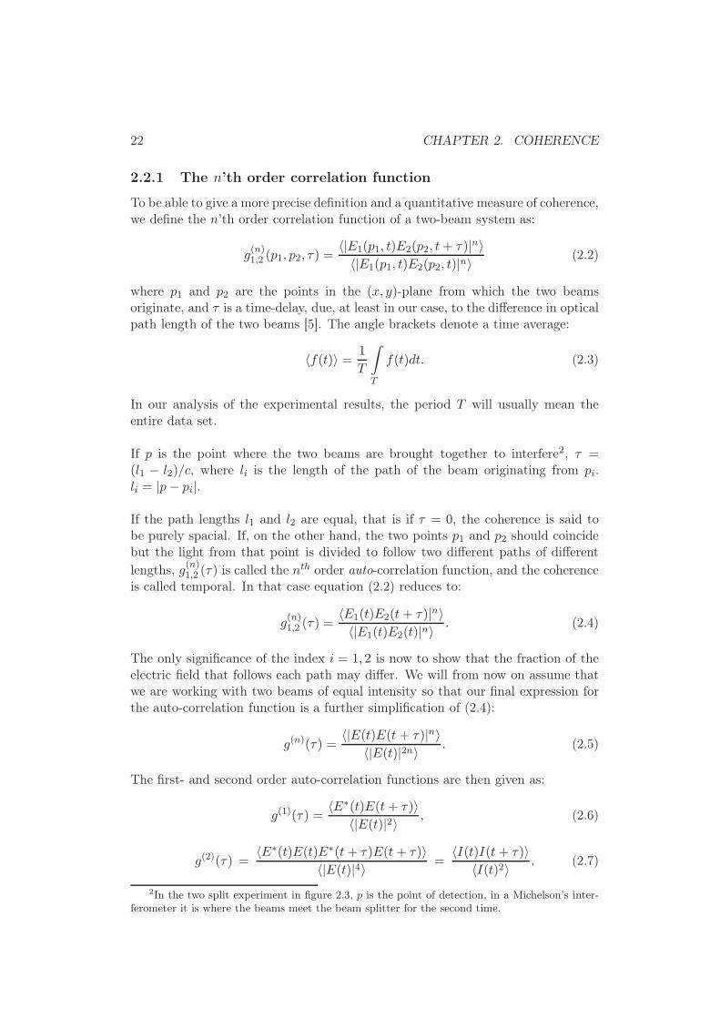
2.2.1 The n’th order correlation function
To be able to give a more precise definition and a quantitative measure of coherence,we define the n’th order correlation function of a two-beam system as:
g(n)1,2 (p1, p2, τ) =
〈|E1(p1, t)E2(p2, t+ τ)|n〉〈|E1(p1, t)E2(p2, t)|n〉
(2.2)
where p1 and p2 are the points in the (x, y)-plane from which the two beamsoriginate, and τ is a time-delay, due, at least in our case, to the difference in opticalpath length of the two beams [5]. The angle brackets denote a time average:
〈f(t)〉 =1
T
∫
T
f(t)dt. (2.3)
In our analysis of the experimental results, the period T will usually mean theentire data set.
If p is the point where the two beams are brought together to interfere2, τ =(l1 − l2)/c, where li is the length of the path of the beam originating from pi.li = |p− pi|.
If the path lengths l1 and l2 are equal, that is if τ = 0, the coherence is said tobe purely spacial. If, on the other hand, the two points p1 and p2 should coincidebut the light from that point is divided to follow two different paths of different
lengths, g(n)1,2 (τ) is called the nth order auto-correlation function, and the coherence
is called temporal. In that case equation (2.2) reduces to:
g(n)1,2 (τ) =
〈E1(t)E2(t+ τ)|n〉〈|E1(t)E2(t)|n〉
. (2.4)
The only significance of the index i = 1, 2 is now to show that the fraction of theelectric field that follows each path may differ. We will from now on assume thatwe are working with two beams of equal intensity so that our final expression forthe auto-correlation function is a further simplification of (2.4):
g(n)(τ) =〈|E(t)E(t + τ)|n〉
〈|E(t)|2n〉 . (2.5)
The first- and second order auto-correlation functions are then given as:
g(1)(τ) =〈E∗(t)E(t+ τ)〉
〈|E(t)|2〉 , (2.6)
g(2)(τ) =〈E∗(t)E(t)E∗(t+ τ)E(t+ τ)〉
〈|E(t)|4〉 =〈I(t)I(t+ τ)〉
〈I(t)2〉 . (2.7)
2In the two split experiment in figure 2.3, p is the point of detection, in a Michelson’s inter-ferometer it is where the beams meet the beam splitter for the second time.

2.2. COHERENCE 23
We will define the n’th order coherence time of a signal to be the time τcoh wherethe absolute value of the envelope of the n’th order correlation function |gn(τ)|has decreased to e−1 of its value at τ = 0, and we say that the signal is n’thorder coherent for τ < τcoh. The coherence length of a signal is defined to belcoh = cτcoh.where c, as always, is the speed of light.
It should be mentioned that the quantity we have called the auto-correlation func-tion often in the literature is named the degree of coherence, while the term temporalcorrelation function or auto-correlation function is reserved for the unnormalizednumerator 〈E∗(t)E(t + τ)〉. Since, as mentioned in the introduction the thesis isonly concerned with relative quantities, we will use the two terms interchangeably.
In reality almost all coherence measurements will be a mix between temporal andspacial coherence, though it may be more spacial than temporal or vice versa. Thedouble slit experiment depicted in figure 2.3 is one example of this. It is onlypurely spacial along the middle line of the interference pattern, where the lengthsfrom the two slits to the screen are the same. For all other points, there willbe a difference in the length of the two paths, and we will therefore have a mixbetween temporal and spacial coherence. In our work, we have assumed that theeffect of temporal coherence is much greater than that of spacial coherence. Whentalking about coherence in the rest of the thesis, it will be implied that we aretalking about temporal coherence. Also, when talking about the first order auto-correlation function, it will simply be referred to as the auto-correlation function.If we are talking about a higher order function, this will be specified.
The second order correlation function can be found directly from experimentaldata using the program in appendix C. The first order correlation function mayseem more tricky, since our detectors measure intensities, not electric fields. In thenext two sections we will look at two methods to determine the first order auto-correlation function of a light source. First, we will see how equation (2.6) maybe re-written to show |g1(τ)| to be equivalent to the earlier mentioned, very usefulexperimental quantity: Visibility, secondly how the auto-correlation function maybe determined by looking at the frequency distribution of the original signal.
Visibility and the first order correlation function
The electric field of the total beam in the previous section is the superposition ofthe electric fields of the two partial beams: E = E(t) + E(t + τ). The detected

24 CHAPTER 2. COHERENCE
intensity is then:
Idet = 〈I(t)〉= 〈|E(t) + E(t+ τ)|2〉= 〈|E(t)|2〉 + 〈|E(t + τ)|2〉 + 〈E∗(t)E(t + τ) + E(t)E∗(t+ τ)〉= 〈|E(t)|2〉 + 〈|E(t + τ)|2〉 + 2Re〈E∗(t)E(t+ τ)〉= 〈|E(t)|2〉 + 〈|E(t + τ)|2〉 + 2|〈E∗(t)E(t+ τ)〉| cos [φ(τ)].
(2.8)
The first two terms in the last line are just the intensity of the two partial beams.Since we have assumed to be working with a 50-50 beam splitter, only half ofthe original incoming intensity takes the path towards the detector3, and we willhave 〈|E(t)|2〉 = 〈|E(t + τ)|2〉 = Ipartial beam = Iin/4. The third term in the lastline in equation (2.8) can be re-written using equation (2.6) with the fact that|E(t)|2 = I(t), so that in the end we find
Idet = 2Ipartial beam{1 + |g1(τ)| cos [φ(τ)]} =Iin2{1 + |g1(τ)| cos [φ(τ)]}. (2.9)
In equation (2.1) we defined visibility to be:
V (∆l) =Imax − Imin
Imax + Imin
If we have a interference maximum at τ−δτ/2, we will have a minimum at τ+δτ/2,where δτ is the time it takes for light to move the distance of one half wave length.In terms of equation (2.9) we may write the visibility as4
V (l) =2I{1 + |g1(τ − δτ/2)|} − 2I{1 − |g1(τ + δτ/2)|}2I{1 + |g1(τ − δτ/2)|} + 2I{1 − |g1(τ + δτ/2)|} ≈ |g1(τ)|, (2.10)
where the last approximation holds if the first order correlation function changesvery little within a time difference of δτ , so that |g1(τ + δτ)| ≈ |g1(τ)|. Since∆l = cτ , writing visibility and the correlation as functions of ∆l or τ is equivalent.First-order coherence may in this case be directly measured through measuring thevisibility of a signal.
The Wiener Khinchine-theorem
The intensity as a function of frequency of a signal of light is known as powerspectral density:
I(ν) = |E(ν)|2 = E∗(ν)E(ν).
3The other half (the light that is twice reflected and twice transmitted in the beam splitter)takes the path back towards the light source. See also the figures 2.4 and 5.9 for an illustrationof this.
4Since cos (φ) will be +1 when I = Imax and −1 when I = Imin.

2.2. COHERENCE 25
If we let E(t) denote the Fourier transformed of E(ν), we have
I(ν) =
∫ ∞
−∞E(t)ei2πνt dt
∫ ∞
−∞E(t′)e−i2πνt′ dt′
=
∫ ∞
−∞
∫ ∞
−∞E(t)ei2πνtE(t′)e−i2πνt′ dtdt′
=
∫ ∞
−∞
∫ ∞
−∞E(t)E(t′)ei2πν(t−t′) dtdt′.
(2.11)
We now define τ to be the difference between t and t′: τ = t − t′. Writingequation (2.11) as a function of t and τ , it becomes
I(ν) =
∫ ∞
−∞
{∫ ∞
−∞E(t)E(t + τ)dt
}
e−i2πντ dτ. (2.12)
Recognizing the quantity inside the curly brackets as part of the definition of theauto-correlation function, equation (2.6) we have5
I(ν) = 〈|E(t)|2〉∫ ∞
−∞g(1)(τ)e−i2πντ dτ.
In other words, the intensity as a function of frequency is (apart from a constant)the Fourier transformed of the first order auto-correlation function. This is knownas the Wiener-Khinchine theorem [24].
2.2.2 Classical theoretical value of coherence length
Following, but somewhat modifying and adapting to our use the method describedby Salamon [43], we will now make a classical estimate of expected coherencelength of light with a Gaussian and Lorentzian frequency distributions. Althoughwe will not make express use of the concept of Fourier transforms, the Wiener-Khinchine theorem will be shown to hold for these cases. It should be stressedthat the Gaussian shape refers to the distribution of the frequency contents in asignal, centered around some central frequency ν0. This distribution is not relatedthe shape of the Gaussian beam described in chapter 1.
General expression for outgoing electric field in a two-beam interfero-
meter
As explained above, in an interferometer, the incoming beam is split, and the par-tial beams follow separate paths until recombined to form an interference pattern.
5One may wonder how we may say that an integral that spans the interval between ±∞ maybe said to be the same as an integral that we specifically defined to be over a period only, as wedid in equation (2.3). However, if the function is not periodic, one period really is infinitely long.If, on the other hand, the function is periodic,taking the integral over many whole periods anddividing by the total number of periods will yield the same answer as if one took the integral overa single period. If the integral is taken over time that is not an integer times the duration of aperiod, any error due to the “leftover” after the last whole will be minute since it will be dividedby the total number of periods.

26 CHAPTER 2. COHERENCE
The electric field of the beam leaving the interferometer is the superposition of theelectric fields of the partial beams. We will again look at only one component ofthe electric field.
Eout =∑
j
Ej .
For a two-beam interferometer, such as the Michelson’s interferometer, this is:
Eout = E1 + E2 = k1Ein(ν)eiφ1(t) + k2Ein(ν)eiφ2(t),
where Ein(ν) is the electric field entering the interferometer, kj is a constant modi-fying the amplitude of the electric field, and φj(t) is the phase of the partial wave.
Detected intensity in a Michelson’s interferometer
Figure 2.4: The path difference in a Michelson’s interferometer will cause a phase difference∆l = 2(l2 − l1) between the two paths.
In a Michelson’s interferometer, each partial wave that leaves the interferometeron the side of the detector will once be reflected and once transmitted through thebeam splitter. Assuming all mirrors to be identical and perfect reflectors, thesewill not affect the constants kj , and any phase change due to the beam splitteror mirrors will be the same for both paths. The phase change due to the beampropagating a length l is given by φ = 2πl/λ = 2πνl/c. Since only the phasedifference between the paths is of any importance, we may write:
Eout(ν) = RTEin(ν)eiφ1 + TREin(ν)eiφ2 = RTEin(ei2πν(2l1)
c + ei2πν(2l2)
c ).
The quantities R and T are the fraction of the original electric field being reflectedand transmitted, and c is again the speed of light. Note that the distance thatenters the equation is actually 2li, since the beam will have to travel the distance

2.2. COHERENCE 27
of the arm twice.
The intensity of the light is -apart from a constant- the absolute square of theelectric field:
Iout(ν) = |Eout(ν)|2 = R2T 2|Ein(ν)|2∣
∣
∣
∣
e
“
i4πνl1c
”
+ e
“
i4πνl2c
”∣
∣
∣
∣
2
.
Assuming a perfect 50-50 beam splitter6 with R2 = T 2 = 1/2 this is7 :
Iout(ν) =1
2Iin(ν)
[
1 + cos
(
2πν∆l
c
)]
,∆l = 2(l1 − l2)
Iin(ν) = |Ein(ν)|2.
The total detected intensity will be the integral of this over all frequencies8:
Idet =1
2
∫ ∞
−∞Iin(ν)
[
1 + cos
(
2πν∆l
c
)]
dν. (2.13)
Coherence length of a light source with a Gaussian intensity distribution
Let us now have a look at the expected coherence length of a light source ofwhich the intensity is a Gaussian function of frequency, centered around a centralfrequency ν0:
Iin(ν) = I0 e−4 ln 2
“
ν−ν0∆ν
”2
, I0 = I(ν = ν0).
The constant ∆ν is called the full width at half maximum (FWHM). If calculatingthe value of the intensity at the points ν0 ± ∆ν/2, one finds:
I(ν0 ± ∆ν/2) = I0/2,
so ∆ν = (ν0 + ∆ν/2) − (ν0 − ∆ν/2) is indeed the width of the intensity graph atthe height where it has decreased to half of its maximum value.
6Half of the intensity reflected, half transmitted.7The energy of a beam of light is proportional to its intensity. Conservation of energy therefore
requires that the sum of the intensity leaving each side of the beam splitter is equal to the incomingintensity. Since intensity is proportional to the square of the electric field, and R and T representthe fractions of the reflected and transmitted electric field, we require R and T squared to beequal to one half for a 50-50 beam splitter.
8Technically, one should weight the frequencies with the detection efficiency P (ν) of thedetector. However, since we will be working with Gaussian and Lorentzian distributions thatgo very fast to zero, and light with a fairly narrow bandwidth, our assumption of a perfect anduniversal detector should be well grounded.

28 CHAPTER 2. COHERENCE
Putting this into the expression for the detected intensity in equation (2.13), wefind9:
Idet =I02
∫ ∞
−∞e−4 ln 2
“
ν−ν0∆ν
”2 {
1 + cos
(
2πν∆l
c
)}
dν
=I04
∆ν
√
π
ln 2
[
1 + exp
{
−1
ln 2
(
π∆l∆ν
2c
)2}
cos
(
2π∆lν0
c
)
]
.
Integrating over all frequencies, we have for the incoming intensity
Iin = I0
∫ ∞
−∞e4 ln 2
“
ν−ν0∆ν
”2
dν =I02
∆ν
√
π
ln 2,
so that the outgoing intensity normalized to that of the incoming is:
Idet
Iin=
1
2
[
1 + exp
{
−1
ln 2
(
π∆l∆ν
c
)2}
cos
(
2π∆lν0
c
)
]
. (2.14)
The intensity has been plotted in figure 2.5. Comparing equation (2.14) withequation (2.9) and (2.10), we see that we have
V (∆l) = exp
{
−1
ln 2
(
π∆ν∆l
2c
)2}
. (2.15)
Above we found that visibility should be proportional to the Fourier transform ofthe intensity distribution I(ν). From Table A.1 we find as predicted:
V (∆l) = exp
{
−1
ln 2
(
π∆ν∆l
2c
)2}
⇀↽ e−4 ln 2
“
ν−ν0∆ν
”2
= Iin(ν).
In this case, the expression for the coherence length is given by:
V (lgcoh) = exp
{
−1
ln 2
(
π∆νlgcoh
2c
)2}
= e−1
⇒ lgcoh =2√
ln 2c
π∆ν.
(2.16)
Coherence light for Lorentzian light
As we will see in chapter 4, the other far side of the possible range of intensitydistributions of atomic light sources is the Lorentzian:
I(ν) = I0∆ν2
4(ν − ν0)2 + ∆ν2,
9We solved the integral by making the substitution u = (ν − ν0)/∆ν, writing the cosine asa sum of exponential functions, and then looking up in [42]. An alert reader may also noticethat the integral is actually the same as the integral solved to find the Fourier transform of theGaussian function, which we solve in appendix A.

2.2. COHERENCE 29
−3 −2 −1 0 1 2 3
0
0.2
0.4
0.6
0.8
1
∆l, relative units
Inte
nsity
rela
tive
units
Figure 2.5: The output intensity of a Michelson’s interferometer using a light source with aGaussian I(ν)-distribution.
where ∆ν is again the FWHM-width of the distribution.
Inserting this into equation (2.13) we have
Idet =I02
∫ ∞
−∞
∆ν2
4(ν − ν0)2 + ∆ν2
[
1 + cos
(
2πν∆l
c
)]
dν.
Looking the integral up in [39] we find:
Idet = I0π
4∆ν
{
1 + e−π∆ν
c|∆l| cos
(
2πν0
c∆l
)}
.
The total incoming intensity is given by
Iin(ν) = I0
∫ ∞
−∞
∆ν2
4(ν − ν0)2 + ∆ν2dν =
I02π∆ν.
This gives a relative intensity of:
Idet
Iin=
1
2
[
1 + e−π∆ν
c|∆l| cos
(
2πν0
c∆l
)]
. (2.17)
The intensity is plotted in figure 2.6.
Again comparing with equation (2.10), we have
V (∆l) = |g1(∆l)| = e−π∆ν
c|∆l|. (2.18)
The coherence length is now:
V (lgcoh) = exp
{−π∆ν
cllcoh
}
= e−1
⇒ llcoh =c
π∆ν.
(2.19)

30 CHAPTER 2. COHERENCE
−3 −2 −1 0 1 2 3
0
0.2
0.4
0.6
0.8
1
∆lrelative units
inte
nsity
rela
tive
units
Figure 2.6: The output intensity of a Michelson’s interferometer using a light source with aLorentzian I(ν)-distribution.
Again comparing with table A.1 we find
1
ω2 + a2⇀↽
π
ae−a|t|.
In finding the auto-correlation function of Gaussian and Lorentzian intensity dis-tribution, we have also shown that the Wiener-Khinchine theorem holds.
In chapter 4, we will have a closer look at the physical meaning of the two shapesof the frequency distribution. We will see that a light source consisting of an ideal,dilute gas will have a Gaussian frequency distribution, while a dense gas of hightemperature will be closer to Lorentzian.
It should perhaps be mentioned that the figures 2.5 and 2.6 have been made forillustrative purposes only, to show the shapes of the expected curves after the lighthas been sent through an interferometer. The curves depicted can hardly be saidto satisfy the requirement that the auto-correlation function (and therefore alsothe visibility) changes very little within a wavelength. With a signal similar tothose depicted, it would be impossible to measure a visibility close to unity evenfor very small ∆l. From equation (2.14) and (2.17), we see that the number ofoscillations within the enveloping curve depends on the ratio R = ∆ν/ν0. If R issmall, the intensity will oscillate fast compared to the damping time of the Gaus-sian or Lorentzian envelope, and the requirement will be satisfied. If R is large,we will have a situation as in figure 2.5 and figure 2.6.
Comparing the coherence length of Lorentzian light sources, equation (2.19), withthat of light of Gaussian intensity distributions, equation (2.16), we see that theGaussian coherence length is a factor 2
√ln 2 larger that the coherence length for

2.3. COHERENCE AS PREDICTABILITY 31
−4 −2 0 2 4
0
0.2
0.4
0.6
0.8
1
Frequency / Hz ν
0 + relative distance
Am
plitu
dere
lativ
e un
its
Figure 2.7: A Gaussian distribution (whole drawn line) has more of its intensity concentratedwithin a narrower FWHM-width, and therefore has a longer coherence length than Lorentziandistributed light (dotted line).
light of a Lorentzian distribution with the same ∆ν. This can be explained byexamining figure 2.7. In Gaussian light, a higher fraction of the total intensity isconcentrated in frequencies between ν0 ± ∆ν/2 than for Lorentzian light.
One could argue that it would make more sense to define a width of the graph thattook this intensity distribution into account, but as we will see, light from physicallight sources tend to be a mix between the two extremes: A pure Gaussian and apure Lorentzian. It is then useful to have a common convention of spectral width.
2.3 Coherence as predictability
Let us again return to the way we described coherence in the introduction, and thatwas repeated at the beginning of this chapter. We claimed that [Coherence timeis] the time τ one may predict the state of a system if one knows its current state.From the above discussion, it should be clear that the predictability in questionis not a matter of whether we are able to mathematically calculate the behaviorof a signal. In that case, the coherence length of a light source would depend onour subjective knowledge of its evolution in time. The predictability is rather aquestion of how sensitive the average intensity of a superposition of a signal witha shifted10 version of itself is. If the intensity is highly dependent on the value ofτ , it is an indication that the signal is highly periodic, and that a change at onepoint of the signal to a great extent is matched by a similar change in the rest ofthe signal. In that sense, the signal may be said to be predictable. If, on the otherhand, the average intensity does not change significantly with different values ofτ , it is an indication that the parts of the signal are not strongly correlated, andthe signal may thus be said to not be predictable.
10In time or space.

32 CHAPTER 2. COHERENCE

Chapter 3
Simulations
In the previous chapter, we saw several examples of relations between quantitiesthat may be calculated from a signal of light. We will now analyze some of theserelations through numerical simulation. We will also try to give an estimate of thecoherence length of the signal, and in the end we will discuss coherence length inrelation to the concept of the photon or quantum of light. The original signals havebeen generated using Matlab-code produced by Borys Jagielski [23]. The analysishas been done using code made by the author, which may be found in appendix C.
Graphs representing quantities that do not in general have magnitudes relative toone have been normalized for easily comparison.
It is worthwhile saying a few words to clarify the terms that will be used. Whenwe talk about a pulse, we will mean the quantity that is emitted from a lightsource, as in figure 3.1. The term wave-packet will be used for a wave envelopedby a function, periodic or not, that groups some of the periods of the wave intoseparate entities, as in figure 3.7(a2)1. In this definition, a pulse will always be awave packet, while a wave packet is not necessarily a pulse.
In the discussion of figures 3.9 and 3.10, we will talk about the background, thepulse-like structure, the central peak and the classical coherence length. The firstterm will refer to the flat background that is especially visible in the last graphin figure 3.9. The second term refers to the larger structure in the background,enveloped by a Gaussian function. The third and fourth terms will both referto the peak of the envelope, a few wave lengths thick, that becomes increasinglydominating and visible for an increasing number of emitters.
1See figure text for letter-labeling of figures.
33

34 CHAPTER 3. SIMULATIONS
3.1 Generation of signals
Generation of all signals builds on a model where light is emitted in the form ofelectromagnetic pulses, or wave-packets as in figure 3.1. Each pulse is a pure sinewith a Gaussian envelope. The author finds this the most intuitive way to picturelight emittance from atoms, as it allows for keeping some ideas from both the waveand particle interpretation of light. It is nevertheless understood that this pictureimposes some strong constraints on the simulations and the interpretation of theirresults.
2.8 3 3.2 3.4 3.6
x 10−13
−0.4
−0.2
0
0.2
0.4
0.6
Time / s
Ele
ctric
fiel
d re
lativ
e un
its
Figure 3.1: An electromagnetic pulse or wave-packet.
To generate a signal in the simulations, the user must choose how many emittersthere will be in the sample, and the probability per data-point for an emitter to emita pulse. Each pulse is characterized by three parameters: Wavelength, amplitudeand damping factor. While the wavelength and amplitude refer to the wavelengthand amplitude of the sine-function mentioned above, the damping factor determ-ines the width of the Gaussian envelope. Each pulse has a sharp value for all threeparameters, but the values vary randomly from pulse to pulse, following a normaldistributed probability function [23]. The generation program allows for the userto determine the central value and width of the distribution function of all threeparameters. In our simulations, we have set the amplitude to be equal to unity forall pulses, that is, with a normal distribution of width equal to zero, The centralwavelengths were chosen to be 633±10 nm or 633±100 nm, corresponding to asmall or large spectral width, respectively (cf. figure 3.8). For the most part, awide spectral width has been used, as the correspondingly short coherence lengthis clearly discernible from the pulse width. The damping factor was set for eachseparate simulation to give the best possible visualisation of the point being dis-cussed. It was, of course, kept constant where required for a fair comparison ofdifferent figures. This applies especially to the figures 3.6 and 3.7, figure 3.11, andfigures 3.9 and 3.10.

3.2. MATLAB CODE FOR ANALYSIS 35
3.2 Matlab code for analysis
We will now give a description of the Matlab code used in the analysis of the gen-erated signals. The code may be found in appendix C, and the line numbering ofthe text refers to the lines in the code.
In the main program, the user is asked to enter the set of data to be plotted, andto choose a τcut (lines 55 and 72 of the code respectively). A τcut is chosen partlyto speed up calculation time, since the loops that generate g(n)(τ) run from ±τcut.The chosen value of τcut should be much smaller than the total length of the dataset to avoid unphysical effects due to low statistics in the end of the function. Ifthe original data does not include a time-column, the user is also asked to statethe sampling time (lines 78-85). The user is then given the following choice:
1. To plot the original signal and its Fourier transform
2. To plot the auto-correlation function of arbitrary order, and its Fourier trans-form
3. To simulate the intensity as a function of the length difference ∆l = cτ in aMichelson’s interferometer, and to plot its visibility
4. To plot power spectral density.
In the following, we will briefly describe the algorithms of the points (2)-(4), thecode of which may be found in section C.3, C.4 and C.5 in the appendix. As inthe code, we will take a to be the amplitude of the original signal, t to be the timein data-points, and τ to be the retardation in time, related to the path difference∆l in an interferometer through ∆l = cτ .
3.2.1 The auto-correlation function
The user is asked to choose the order n of the auto-correlation function (cf. thedefinition of g(n)(τ) on page 22), and the nth order auto-correlation function isgenerated (lines 193-212). In generating g(n)(τ), a loop runs between the valuesτ = ±τcut. The auto-correlation function is then calculated as a(t)×a(t+τ) for allt in the interval defined by τcut from each end of the total data set. The programwill also calculate the Fourier transform of g(n)(τ) (lines 238-242), which the useris offered to save (lines 248-257) for later comparison with the visibility function(cf. equation (2.10)).
If the user has chosen to plot the first order auto-correlation function, the programautomatically also finds and plots its absolute value, and offers to save the inform-ation for later comparison with the power spectral density (lines 250-286).

36 CHAPTER 3. SIMULATIONS
3.2.2 Simulation of a Michelson’s interferometer
The algorithm is similar to that of the auto-correlation function, but this timecalculating the sum (instead of the product): a(t) + a(t+ τ) (lines 303-309). Theoutput intensity is the square of this, normalized by the intensity at τ = 0.
To find the visibility, we defined two vectors, pks_n and pks_p where we enteredthe minimum and maximum values of the intensity function (lines 321-323). Avisibility-vector was defined as visibility(i) = (pks_p(i) - pks_n(i))/(pks_p(i) +pks_n(i)), with i being the element number of the vectors (line 337). The positionof visibility(i) was defined as the mean value of the positions of pks_n(i) andpks_p(i) (lines 335-337). The program offers to save the visibility graph for latercomparison with the absolute value of the Fourier transform of the first orderauto-correlation function (lines 347-355).
3.2.3 Power spectral density
The user may choose to divide the original signal into a number of sub-segments(line 359). The program then calculates the Fourier transform of the square ofeach sub-segment separately, and superposes them (lines 379-389). If the numberof sub-segments is chosen to be high, the average obtained from sub-segmentingwill be better, but at the cost of adding to the edge-effects and effects stemmingfrom decreased statistics, of each Fourier transform due to shorter segments. Sub-segmenting should not be used if the original data is not stationary.
3.3 The Wiener-Khinchine theorem
On page 24, we showed that power spectral density is equal to the Fourier transformof the first order auto-correlation function. In figure 3.2, we have plotted thepower spectral density described in section 3.2.3 in red together with the Fouriertransform of g1(τ) from section 3.2.1 in blue.
In the figure, a sub-segmenting of 14 was used to obtain the graph of the spec-tral density. The upper frame shows the calculated Fourier transform. In thelower frame the graphs have been smoothed using the built-in Matlab-functionsmooth(data,n), where data is the set of data that is to be smoothed, and n is aninteger. The function smooth makes a moving average of n points around eachdata point in data.
As seen in the figure, our signal is in very good agreement with the theoreticalprediction that says that g(1)(τ) ⇀↽ I(ν) (equation (2.12)). The curve describ-ing spectral density has slightly lower values than the curve generated from theauto-correlation function. Examining the upper figure, the red line has one peaksignificantly higher than the rest, and in using the very simple normalization of

3.4. VISIBILITY AND THE AUTO-CORRELATION FUNCTION 37
0 2 4 6 8 10
x 1014
0
0.2
0.4
0.6
0.8
1
Frequency / Hz
Rel
ativ
e am
plitu
de
Figure 3.2: Numerical test of the Wiener-Khinchine theorem
defining the highest peak to be equal to one, this will cause the bulk of the curveto be shifted towards lower values.
3.4 Visibility and the auto-correlation function
The first frame in figure 3.3 shows the first order correlation function of the signal(cf. section 3.2.1), the second the intensity as as function of τ = c∆l that one wouldobtain if sending the light through a Michelson’s interferometer, as described insection 3.2.2. If one neglects the fact that the second graph is shifted to haveonly positive values (since the intensity cannot be negative), the two graphs areidentical2. Comparing the third line of equation (2.8), which shows the intensityfrom an interferometer, with equation (2.6) defining the first order correlationfunction, this is not surprising3.
2As in chapter 2 we have normalized the intensity to that of the incoming intensity3In a Michelson’s interferometer, it does not matter which arm is defined to give the electric
field E(t) and which arm gives the field E(t+τ ). This is equivalent to saying that the the intensityof the light from an interferometer should be the same for positive and negative τ . We may thenwrite 〈E∗(t)E(t+τ )+E(t)E∗(t+τ )〉 = 〈E∗(t)E(t+τ )+E(t)E∗(t−τ )〉 = 〈E∗(t)E(t+τ )+E∗(t−

38 CHAPTER 3. SIMULATIONS
−1 −0.5 0 0.5 1
x 10−13
−1
−0.5
0
0.5
1Autocorrelation function
τ / s
g1 (τ)
−1 −0.5 0 0.5 1
x 10−13
0
0.5
1Intensity after Michelsons interferometer
tau / s
Rel
ativ
e in
tens
ity
Figure 3.3: The shape of the intensity as a function of τ = c∆l from a Michelson’s interferometeris identical to the shape of first order correlation function, but their absolute values are different.
On page 23 we showed that the absolute value of the first order correlation functionis equal to the visibility. In figure 3.4 we have plotted the absolute value of the auto-correlation function together with the visibility of the same signal as in figure 3.3.Again, our simulations are in good agreement with the theory.
τ )E(t)〉. Making the shift t′ = t− τ this is: 〈E∗(t)E(t+ τ )+E(t′)E∗(t′ + τ )〉 = 2〈E∗(t)E(t+ τ )〉,where the last equation is valid because we are taking the integral over all t. The two equationsmentioned in the paragraph are now directly comparable.

3.4. VISIBILITY AND THE AUTO-CORRELATION FUNCTION 39
−1 −0.5 0 0.5 1
x 10−13
0
0.2
0.4
0.6
0.8
1
τ /s
rela
tive
ampl
itude
|g1(τ)|
Visibility
Figure 3.4: The visibility is equal to the absolute value of the first order auto-correlationfunction |g1(τ )|.
0 1 2 3 4
x 10−12
−1
−0.5
0
0.5
1
3 emitters
Time / s
Ele
ctric
fiel
d re
lativ
e un
its
0 1 2 3 4
x 10−12
−1
−0.5
0
0.5
1
30 emitters
Time / s
Ele
ctric
fiel
d re
lativ
e un
its
0 1 2 3 4
x 10−12
−1
−0.5
0
0.5
1
Time / s
Ele
ctric
fiel
d re
lativ
e un
its
300 emitter
Figure 3.5: When the number of emitted pulses become large, the pulse pattern graduallybecomes hidden in the interference pattern of superposed pulses.

40 CHAPTER 3. SIMULATIONS
3.5 Wave packets, photons and coherence length
As it was briefly mentioned in the introduction, some authors seem to suggestthat the coherence length of a signal may be identified as the size of a photon orquantum of light [2], [25]. In our model, this size would intuitively correspondto the dimensions of the curve enveloping the pulse in figure 3.1. We will inthe following examine some methods of determining coherence, and see how thecoherence length depends on the number of emitters.
3.5.1 Does the coherence length correspond to the photon size?
In chapter 2, the coherence length and time of a signal was defined to be the∆l = cτ where the value of the auto-correlation function had decreased by a factore−1. This definition was shown, theoretically and numerically to be equivalentwith the half-width of the visibility function. Other ways of finding the coherencetime of a signal have been suggested, some have also been proved. In this section,we will numerically examine the following methods of calculating coherence time:
1. The size of a photon, which in our pulse-model would correspond to thetemporal length of a pulse
2. The width of the visibility function
3. Calculation from the width of the power spectral density, according to theclassical value for a Gaussian intensity distribution.
We have chosen to use the visibility function rather than the auto-correlation sincewe have shown that the two are equivalent, and it is easier to make a rough estim-ate of the former through examination of figures 3.6 and 3.7.
Examine for a moment figure 3.6(a) and figure 3.7(a1 and a2). The only differencebetween the two figures is the number of light emitters; figure 3.6 depicts a singlelight pulse from a single emitting atom, while figure 3.7, shows a signal that is a su-perposition of pulses from one hundred emitters4. The pulse in 3.6 has a e−1-widthof about 0.35 × 10⁻¹² sec, the value of the visibility graph, figure 3.6(d), when itsamplitude is e−1 is about 0.25 × 10⁻¹², that is in the same order of the pulse.The signal in figure 3.7(a2) also shows a wave-packet pattern, but this time onewave-packet lasts for a much shorter time; a rough estimate gives 0.01× 10⁻¹² secper wave-packet. Again, the number is approximately equal to that found throughan examination of graphs showing the visibility function, figure 3.7(d).
According to the results found in chapter 2, the coherence length of a source of aGaussian frequency distribution is
lgcoh =2√
ln 2c
π∆ν⇒ τ g
coh =2√
ln 2
π∆ν, (3.1)
4As described in section 3.1, each emitter has a given probability per data point of emittinga pulse. If a signal contains n pulses, the pulse density is such that there are n pulses within adistance lmax = cτmax, where lmax is the maximum length difference of the interferometer.

3.5. WAVE PACKETS, PHOTONS AND COHERENCE LENGTH 41
2.8 3 3.2 3.4 3.6 3.8 4 4.2 4.4
x 10−12
−1
0
1
Original signal
Time / s
Ele
ctric
fiel
d r
elat
ive
units
3.85 3.9 3.95 4 4.05 4.1 4.15
x 1014
0
0.5
1
Fourier transform of original signal
Frequency / Hz
Rel
ativ
e am
plitu
de
−4 −3 −2 −1 0 1 2 3 4
x 10−13
−1
0
1Autocorrelation function
τ / s
g1 (τ)
−4 −3 −2 −1 0 1 2 3 4
x 10−13
0
0.5
1Visibility after Michelsons interferometer
τ / s
Vis
ibili
ty
3.85 3.9 3.95 4 4.05 4.1 4.15
x 1014
0
0.5
1
Power spectral density
Frequency /Hz
Rel
ativ
e am
plitu
de
Figure 3.6: A single pulse. From the top down: (a) Electric field, (b) Fourier transform of theelectric field, (c) auto-correlation function, (d) visibility and (e) power spectral density.

42 CHAPTER 3. SIMULATIONS
0 0.5 1 1.5 2 2.5 3 3.5
x 10−12
−10
0
10Original signal
Time / s
Ele
ctric
fiel
d re
lativ
e un
its
1.35 1.4 1.45 1.5 1.55 1.6
x 10−12
−5
0
5Original signal
Time / s
Ele
ctric
fiel
d re
lativ
e un
its
0 0.5 1 1.5 2
x 1015
0
0.5
1
Fourier transform of original signal
Frequency / Hz
Rel
ativ
e am
plitu
de
−8 −6 −4 −2 0 2 4 6 8
x 10−14
−1
0
1
Autocorrelation function
τ / s
g1 (τ)
−8 −6 −4 −2 0 2 4 6 8
x 10−14
0
0.5
1Visibility after Michelsons interferometer
τ / s
Vis
ibili
ty
0 0.5 1 1.5 2
x 1015
0
0.5
1
Power spectral density
Frequency / Hz
Rel
ativ
eam
plitu
de
Figure 3.7: A superposition of one hundred pulses. From the top down: (a1) Electric field, (a2)enlarged section of the electric field, (b) Fourier transform of the electric field, (c) auto-correlationfunction, (d) visibility and (e) power spectral density.

3.5. WAVE PACKETS, PHOTONS AND COHERENCE LENGTH 43
The FWHM-width of the power spectral density of the single pulse is approx-imately ∆ν = 0.021 × 10¹⁴ Hz. Plotting this value into equation (3.1) gives atheoretical value of the width of the visibility graph:
τ gcoh =
2√
ln 2
π∆ν=
2√
ln 2
0.021 × 10¹⁴π Hz= 0.25 × 10⁻¹² sec, (3.2)
in exact agreement with the above estimate.
The width of the power spectrum of the light from the hundred emitters is harderto define, but a value of 0.2 × 10¹⁵ Hz seems to be of the right order. The shapeof the spectrum may hardly be said to be a well defined Gaussian, but in lackinga proper expression, we will use equation (3.1). We then find:
τ gcoh =
2√
ln 2
π∆ν=
2√
ln 2
0.2 × 10¹⁵π Hz= 0.27 × 10⁻¹⁴ sec, (3.3)
As expected, the match is not as good as for the single graph. The coherencelength found from the width of the pulse is a little less than a factor 4 longerthan that found from the power spectral density. The disagreement may be dueto the fact that the power spectral density is composed of several distinct peaks,which together would not decrease the coherence length as much as our roughlydetermined FWHM suggests.
As mentioned at the beginning of this section, the only difference between the twosets of graphs in figure 3.6 and figure 3.7 is the number of light emitters. Seeingthe difference between the coherence lengths in the two cases, it is very difficult toexplain how coherence length may correspond to the size of a photon unless one iswilling to sacrifice the idea of a photon as an indivisible and unique link betweentwo events (cf. the introduction chapter) [19]. If one, on the other hand is willingto see the photon as a statistical feature arising from the superposition of severalpulses of electromagnetic radiation, the picture of light in the form of particlesor wave-packets may be kept, and the photon may then be identified as the wavepackets defined in the introduction of this chapter. In the case of a single pulse,the photon will be identical to a pulse, while in the case of many such pulses asin figure 3.7(a2), we will be forced to identify the photon as the wave packets ofmuch shorter coherence length than each original pulse.
It may be clarifying to briefly return to the analogy that opened our descriptionof interference in chapter 2. In the case of a single pebble being thrown into thequiet lake, the waves that emerged could truly be said to stem from that pebblehitting the water. In the case of many such pebbles, there is no longer a one-to-one link between a specific pebble to a resultant wave-top far from where thepebbles hit. Each wave-top5 is a superposition of a collection of original waves,and each original wave may be part in the formation of several such new wave-tops.
5It may be confusing that a photon now corresponds to a wave in water, but hopefully thereader is able to understand the analogy.

44 CHAPTER 3. SIMULATIONS
−1.5 −1 −0.5 0 0.5 1 1.5
x 10−12
0
0.2
0.4
0.6
0.8
1
τ / sec
visi
bilit
yOne pulse
−3 −2 −1 0 1 2 3
x 10−14
0
0.2
0.4
0.6
0.8
1
τ / sec
Vis
ibili
ty
100 pulses
Figure 3.8: The visibility, and therefore the coherence length of single pulses is highly dependenton the length of the pulse. When the number of pulses increases, the coherence length no longerdepend on this length. Note the color/pattern coding of the graphs and the difference scaling ofthe τ -axis.
In figure 3.8, the dependence of coherence length on pulse size and line width isfurther investigated. The upper frame depicts the visibility of single pulses. Aswe saw and discussed in the previous paragraphs, the coherence length of a singlepulse is comparable to the length of the pulse. The second graph in figure 3.8depicts the coherence length of light from one hundred emitters with the samestatistical settings as for the pulses in the upper graph.
In both sub-figures in 3.8, the damping factor (corresponding to the temporal sizeof a pulse) of the blue and dashed gray pulse is the same, while the damping factorof the black pulse is significantly longer. On the other hand, when it comes to thestatistical properties of a collection of pulses, the picture is another: The black andthe dotted gray lines both have a standard deviation of wave length of 100 nm,while the blue has a standard deviation of 10 nm. In all three cases, each single

3.5. WAVE PACKETS, PHOTONS AND COHERENCE LENGTH 45
pulse contains only one wavelength6, but the probability for a pulse to be emit-ted with a given wavelength follows a Gaussian probability distribution with thestandard deviations just mentioned. In each case, this distribution is centered at633 nm, the nominal wave length of our laser.
As implied from the previous paragraph, the statistical properties of the pulses donot matter in figure 3.8(a). When comparing with figure 3.8(b), however, it be-comes clear that the standard deviations are important, as it is the two graphs withthe same standard deviation that have similar widths. In our case, the collectiveproperties are very dominant for the signal from 100 pulses. It should not be for-gotten that the Fourier transform of the signal and the power spectral density willdepend on both the damping factor and standard deviations of the wavelengthsIt would be interesting to see how varying the values of these would change thegraphs in 3.8. Standard deviations of 10 and 100 nm are rather large, and willtherefore tend to make the coherence length of the light very short. The physicalmeaning of a given standard deviation will be further investigated in chapter 4.
The auto-correlations function of an increasing number of emitters
Let us again look at the auto-correlation function of the pulse-signal, this timeover a larger range of τ . Figure 3.9 shows the absolute value of |g1(τ)| for lightemitted from 10, 100, 1000, and 10000 atoms. Figure 3.10 shows the same graphszoomed in on the central maximum. The auto-correlation function seems to have aless defined value. Even with as many as 1000 emitters, there is a structure higherthan than the flat background but not belonging to the central peak. The widthof the structure is of the same order as in the figures for 10 and 100 emitters, soit seems natural to assume that the structure stems from the shape of the originalpulse. The value of the highest point of this structure is decreasing with an increas-ing number of emitters, until it is barely discernible when the number of emittersbecomes very large. At the same time, the fluctuations of the background seemto increase, and comparing the two lowest frames in figure 3.9, it does not seemimpossible that it reaches a constant level, and that this level is reached when thenumber of emitters become large enough for the pulse-structure to be indiscernible.
Examining the figures 3.8 and 3.10, it looks like the width of each of the small topsof the fluctuations in the background are of approximately the same width as thecentral maximum.
Figure 3.9 and 3.10 seem to contain more information than what we have seen con-tained in the auto-correlation function discussed in the literature. An experimentalverification of the pattern shown in the figures would significantly strengthen the
6Strictly speaking, a pulse is never entirely monochromatic, since, according to the discussionof Fourier transforms in appendix A that would imply that the length of it is infinite, and it wouldno longer be a pulse. What we mean is that the wavelength “inside” the pulse is well-defined.

46 CHAPTER 3. SIMULATIONS
−1 0 1
x 10−11
0
0.2
0.4
0.6
0.8
1
τ / s
|g1 (τ
)|
10 emitters
−1 0 1
x 10−11
0
0.2
0.4
0.6
0.8
1
τ / s
|g1 (τ
)|
100 emitters
−1 0 1
x 10−11
0
0.2
0.4
0.6
0.8
1
τ / s
|g1 (τ
)|
1000 emitters
−1 0 1
x 10−11
0
0.2
0.4
0.6
0.8
1
τ / s
|g1 (τ
)|
10000 emitters
Figure 3.9: The absolute value of the first order auto-correlation function for 10, 100, 1000 and10000 emitters.

3.5. WAVE PACKETS, PHOTONS AND COHERENCE LENGTH 47
−5 0 5
x 10−14
0
0.2
0.4
0.6
0.8
1
τ / s
|g1 (τ
)|10 emitters
−5 0 5
x 10−14
0
0.2
0.4
0.6
0.8
1
τ / s
|g1 (τ
)|
100 emitters
−5 0 5
x 10−14
0
0.2
0.4
0.6
0.8
1
τ / s
|g1 (τ
)|
1000 emitters
−5 0 5
x 10−14
0
0.2
0.4
0.6
0.8
1
τ / s
|g1 (τ
)|
10000 emitters
Figure 3.10: The absolute value of the first order auto-correlation function for 10, 100, 1000and 10000 emitters, zoomed in on the central maximum.

48 CHAPTER 3. SIMULATIONS
pulse model of light emission7 As shown on page 37, the first order auto-correlationfunction of a signal is equal in shape to the signal from a Michelson’s interfero-meter, and measurements should in principle be possible.
A few words should be said on the attenuation of a beam of light down to verylow intensities. One may perceive the attenuation of a beam in at least two ways.
1. The shape of the signal remains the same as when the intensity was higher,but the amplitude is scaled down gradually as the attenuation factor increases
2. Decreasing the intensity would cause the signal to become a superposition offewer pulses, and it would therefore regain the pulse-like appearance we sawin figure 3.5.
The first option is closely related to a classical wave-description of light, the secondfavours a quantum description where the pulses emitted from atoms are indivisiblephotons. It is possible to argue that the method chosen to attenuate the beamwould play a significant part. If the intensity of the light source itself is lowered, itseems natural that one would return to a pulse-like signal8. If, on the other hand,the light source is kept at a constant intensity and the beam is attenuated using afilter, both of the possibilities i and ii seems perceivable. Experimentally, a directmeasurement of a beam at very low intensities is difficult, since it would requireusing a detector similar to our SPCM-detector which by its nature has single pulsesas output (see chapter 5 for a discussion of the SPCM). Using the auto-correlationfunction instead of the raw signal, it may be possible to distinguish between thetwo.
In figure 3.9, the value of the maximum point of the pulse shaped background isdecreasing with an increasing number of emitters. When the number of emittersbecomes very large, this background is no longer visible. In figure 3.11 we haveplotted the maximum value of the background as a function of the number ofemitters9. The graphs seems to be decreasing towards a constant value. It seemsnatural that a function describing the graph in the figure would be a function ofthe number density, damping factor and wavelength of the pulses. In the figure,we have included a curve fit on the form A = a/(n+b) where A is the amplitude ofthe graph at point n, and a and b are constants. A function on the form of a simplefraction was chosen from purely visual arguments, as it seemed to give a better fitthan an exponentially or logarithmically decreasing function, or more complicatedfractions of polynomials. Intuitively, in light of the arguments above, it seems as if
7Given, of course, that one is not able to find another model that predicts the same behaviour.8It is implied that the energy of each pulse remains the same, so that the decrease of intensity
is due to a lowering of the number of pulses emitted.9The reader should be warned that the original code was meant simply to visualize the auto-
correlation function, and consequently did not include a way of calculating any numerical values.The values in the graph are the maximum value of a Gaussian function that was visually fittedto the pules-structure. Accordingly, the values given are due to the (possibly large) correctionfactor of a human being that would like to be right.

3.5. WAVE PACKETS, PHOTONS AND COHERENCE LENGTH 49
0 2000 4000 6000 8000 10000
0
0.5
1
Number of emitters (n)
Rel
ativ
e am
plitu
deof
pul
se−
like
stru
ctur
e
Numerical dataCurve fit on form a/(n+b)
Figure 3.11: The maximum value of the background as a function of the total numbers ofemitters.
a function on the form of a simple fraction would not be complete, since it does nottake the flat background into account, but becomes equal to zero as the numberof emitters, n, approaches infinity. A separate constant or slowly increasing termdescribing the background could be added to make up for this. Unfortunately, timedid not allow us to make the necessary theoretical speculations or simulations togive other hints of the dependence on the factors suggested above.
Increasing the number of emitters, and therefore the intensity of the light cor-responds to moving from the quantum mechanical to the classical domain. If thebehaviour suggested in figure 3.11 is confirmed by experiment, the coherence lengthcould be a measure of the extent to which a system belongs to the quantum ofclassical domain.
Pulse-shape
As described at the beginning of the chapter, the models we use are based onpulses with a Gaussian envelope. It would be interesting to repeat the analysisof the previous sides with different-shaped pulses. Two possibilities would be tochoose a square envelope as in figure 3.12(a), or an exponentially decaying envelopeas in figure 3.12(b). The second of these would perhaps be the more interestingfor two reasons: 1) It is probably more physical than a box-shape, as it couldbe directly related to the quantum mechanical state function that we will findin chapter 4, and 2) we predicted in chapter 2 that the auto-correlation functionis symmetric around τ = 0. Using an un-symmetric pulse-shape would possiblyshow some interesting features. On the other hand, doing the simulations withsimple pulse-shapes, such as a box, would allow us to investigate closer the shapeof the pulse-structure of the auto-correlation. In that respect, the Gaussian envel-ope we chose is maybe a little too well-behaved for all details to emerge in the plot.

50 CHAPTER 3. SIMULATIONS
0 1 2 3 4
−1
−0.5
0
0.5
1
Relative time
Ele
ctric
fiel
dre
lativ
e un
its
0 1 2 3 4 5 6−1
−0.5
0
0.5
1
Relative time
Ele
ctric
fiel
dre
lativ
e un
its
Figure 3.12: Possible interesting pulse-shapes for future simulations: (a) A square box, and(b) and exponentially decreasing function.
Problems with a common definition of coherence time
Some authors define coherence time to be [44]
τc =
∫ ∞
−∞|g(1)(τ)|2dτ. (3.4)
This is a definition that works for functions that decrease to zero fast enough forequation (3.4) to be well defined. If, on the other hand the fluctuations appearingin our simulations should prove to be aspects of a physical reality, not only dueto the limitations of numerical simulation, the integral in (3.4) will diverge. Toresolve this problem, we see two possible solutions:
1. To redefine coherence time and length to include the width of the central

3.5. WAVE PACKETS, PHOTONS AND COHERENCE LENGTH 51
peak only, make a fit of the peak with a function f(τ) of which the integralτc =
∫∞−∞ |g(1)(τ)|2dτ is well defined, and define this to be the true expression
for the coherence time.
2. To introduce a cut-value τcut and redefine the coherence time to be
τc =
∫ τcut
−τcut
|g(1)(τ)|2 dτ. (3.5)
The first approach seems unsatisfactory in that it neglects some possibly import-ant features of the auto-correlation function. Having to fit a graph with an almostfreely chosen function also introduces an element of subjectivity into the definition,as the choice of function may not be obvious. By examining the uppermost graphsin the figures 3.9 and 3.10 it is also not obvious how to make such a fit for signalsfrom very few emitters.
The second approach allows for the inclusion of features apart from the centralmaximum to be included in the definition of coherence length, given that one isable to make a sensible choice τcut. Using the wave-packet structure in figure 3.9as a basis may open for a definition of τcut less arbitrary than what has hithertobeen possible. One possibility is to define that:
The cut value τcut should be equal to the value of τ where the the en-velope of pulse-structure is a factor κ1 larger than the average value ofthe background when the number of emitters approaches infinity. If thetop of the pulse structure is smaller than a factor κ1 times the averageof the background, τcut should be at the position of this first minimumafter the central peak.
A definition of τcut similar to the definition above would allow for inclusion of fea-tures of the auto-correlation function aside from the central maximum, and beingwell defined even for a signal with many fluctuations in the auto-correlation func-tion.
Another possible way to define τcut would be to find the enveloping curve for somevery few emitters, choose a cut value where the curve is equal to some κ2, andkeep that value of τcut constant regardless of the number of emitters. This defini-tion would in practice probably be more time consuming, since it would require aknowledge of the auto-correlation function of a single or very few pulses.
On the other hand, it could well be argued that if we have already found a char-acteristic time τcut of a graph, then τcut itself could well be used as a definition ofcoherence time, and the integral in (3.5) would be superfluous.

52 CHAPTER 3. SIMULATIONS
Chapter 4
Components of the experimental
setup
“There is another much stronger motive which fascinates the good sci-entist in connection with practical application, namely: to see that isworks; to see that one has correctly understood nature” (Werner Heis-enberg in [21]).
As the choice of opening quote suggests, one of the author’s fascinations with thenatural sciences is nature’s ability to be described in the language of mathematics,and the possibility to make predictions for practical application based on the rulesof that language1. It was to a large part this fascination that motivated the presentchapter.
4.1 Spectral lamps
The structure of the atom, and why an atomic element emits light of
certain wavelengths
Examining the colors of light emitted from matter under certain conditions is anold and effective technique of identifying chemical elements. The wavelengths ofthe visible spectral lines of the hydrogen atom was mathematically described byJohann Balmer in 1885, and in the years that followed, descriptions of other linesin the non-visible part of the spectrum were added.
At the beginning of the 20th century, Max Planck presented his idea of quantiza-tion of energy to explain the black-body spectrum, and shortly thereafter AlbertEinstein suggested that the electromagnetic field itself is quantized into what isnow known as photons. Experiments showing the photoelectric effect2 were seen
1Whether she may be counted among the good scientists is a question subjective in naturethat the author herself will not attempt to answer. The fascination, however, remains.
2The photoelectric effect is the phenomenon that electromagnetic radiation hitting a metalplate will cause electrons to loosen, and therefore create an electric current if and only if the
53

54 CHAPTER 4. COMPONENTS OF THE EXPERIMENTAL SETUP
as hard proof of these particles of light3.
In 1913 Bohr introduced his model of the atom in which he used Planck’s idea ofquantization of energy to explain the mechanism behind the observed wavelengthsin the hydrogen spectrum. The idea was that the electron moves around the nuc-leus in circular orbits, the radius of which corresponds to a given energy. In thetransition from a larger to a smaller radius, the atom loses energy which is emittedin the form of quanta of electromagnetic radiation.
Although a tremendous achievement and a great leap forward for theoretical phys-ics, several steps in the derivation of Bohr’s formula were highly questionable4, themost fundamental of which was the way he used classical mechanics to find thestable energy levels. Nevertheless, the idea that the spectrum has something to dowith the energy of the electrons in the atom was born [52].
Inspired by classical wave mechanics and Louis de Broglies idea that matter may beassigned a wavelength, Erwin Schrödinger invented a wave equation for quantummechanics, the validity of which was proven through experiments [17].
Light can be emitted from or absorbed in an atom if the energy of the light cor-responds to the energy difference between two of the atomic energy levels allowedby the Schrödinger equation.
ih∂ψ
∂t=
(
− h2
2m∇2 + V
)
ψ = Eψ, (4.1)
where ψ is the state, V is the potential, m the mass, and E the energy of thesystem we are working with. For electrons belonging to an atom in a gas wherethe interactions between the separate atoms may be neglected, the potential canbe assumed to be the total coulomb potential of the protons in the nucleus plusthat of the other electrons. It is typically only the valence electrons of an atomthat undergo optical transitions [44].
For atoms of chemical elements, the solutions to (4.1) are discrete. The light thatis emitted from an atom can therefore have only certain wavelengths determinedby the difference between the energy levels of the atom, as given by Planck’s law:
ν =∆E
2πh=E2 − E1
2πh, (4.2)
quantity 2πhν where ν is the frequency of the radiation is larger than the binding energy of theelectron. A voltage V0 may be set up in the other direction to prevent the current. This voltage isonly dependent on the frequency, and not on the intensity of the light [52] (see also the discussionof equation (4.2)).
3Whether the photoelectric effect is really a proof of the particle nature of light has later beenquestioned. See for example the discussion of the effect in [22].
4That is, highly questionable to the modern physicist familiar to the rules of quantum mech-anics.

4.1. SPECTRAL LAMPS 55
Figure 4.1: The spectra of our gas discharge lamps. From the top down: White light, neon,argon, mercury, and mercury lamp with interference filter (for a brief discussion on interferencefilters, see section 4.2). The camera settings were adjusted to give each separate picture the bestpossible quality. The relative intensities may therefore not be compared between two differentphotographs. The circle around the bright green line in the mercury spectra is a reflection of thelamp holder (photographs by author).
E1 and E2 being the energies of the higher and lower electron level. As a resultof this, each element has a spectrum of possible wavelengths, something that isreflected in figure 4.1 for Neon, Argon and Mercury. The uppermost photographin figure 4.1 shows the spectrum of white light.
4.1.1 Broadening mechanisms
From our discussion of the energy levels of the atom, one could think that thefrequency of each spectral line of the emitted radiation would have a sharp value.This is not the case even in principle. The mechanisms that govern the spectralwidth of the intensity function of each line are called broadening mechanisms. Itis common to distinguish between two main families of broadening mechanisms:Homogeneous broadening, that affect all the separate microscopic light sources(that is, all atoms) in the same way, and inhomogeneous broadening due to actualdifferences between the light sources, and to the statistical properties of the col-lection of sources.
As we will see, homogeneous mechanisms give rise to a Lorentzian shaped intensityfunction, whereas inhomogeneously broadened lines of ideal gases are Gaussian [44].
Lifetime broadening
In the formalism of quantum mechanics, a physical state may be written as5
ψ(t) =∑
n ψn(t), where the ψn’s constitute a complete set of basis-vectors. Ameasurement of a property, or physical observable A of ψ(t) may be described
5In anticipation of the calculation of natural linewidth, we have chosen not to normalize theψn’s to have length equal to unity.

56 CHAPTER 4. COMPONENTS OF THE EXPERIMENTAL SETUP
through an operator A acting on the state. The Dynamics of ψ(t) may be said tofollow two main principles [8]:
1. The wavefunction ψ(t) evolves continuously and deterministically accordingto the Schrödinger equation (equation (4.1)). The Schrödinger equation islinear so that if ψ(t) and φ(t) are solutions, then αψ(t)+βφ(t), where α andβ are constants, will also be a solution.
2. Upon a measurement, the state ψ(t) is discontinuously reduced to some ψ′n
which is an eigenvector of the operator describing the measurement, and themeasurement will return the corresponding eigenvalue an. The reduction isstochastic, not deterministic. The probability of obtaining an is equal to theabsolute square of ψn; P (an) = |ψ′
n|2.
According to the second dynamic principle of quantum mechanics, a measurementof a single quantum system will necessarily return one of the eigenvalues of thesystem, and the state will collapse to the corresponding eigenvector ψn(t). It istherefore impossible to find the total original state ψ(t) doing measurements ononly one quantum system. Since after a measurement the state of the system willbe changed, repeated measurements on the same system will be void6.
Heisenberg’s uncertainty principle of position and momentum states that
∆x∆p ≥ h
2,
where ∆x = σx and ∆p = σp are the standard deviations of the data-set of multiplemeasurements or position and momentum on identical sets of quantum systems7.A similar uncertainty principle holds for time and energy:
∆t∆E ≥ h
2. (4.3)
In this case, the interpretation that “∆” really means the standard deviation ofrepeated measurements is problematic. Time is a running parameter, not a dy-namical variable8. There is no time-operator, you simply cannot measure the timeof a system! How then should we understand ∆t?
6It is far beyond our aim to discuss the problem of the reality of the wavefunction. Whetherthis collapse of the wavefunction is something that happens within the state itself or only in ourknowledge of the state, has been, and is still, a matter of dispute.
7Actually, in the standard interpretation of quantum mechanics, σA is the standard deviationof the quantum system itself. Quantum mechanics states that one cannot measure every propertywith arbitrarily good precision at the same time. This is closely related to the theory of Fouriertransforms. The sets of position- and momentum eigenstates are Fourier pairs. If the position of astate is measured, the wavefunction will become a delta function in the position-state. Accordingto table A.1, the wavefunction will then become a constant in momentum space, its standarddeviation will become infinite, and we will not know anything about the momentum of the state.At this point, however, we have gotten dangerously close to breaking our promise of not discussingthe reality of the physical meaning of ψ(t).
8Assuming that we stay clear of relativistic quantum mechanics.

4.1. SPECTRAL LAMPS 57
To answer that question, we will need to look at the other input in equation (4.3):∆E. This is again a variable to which repeated measurements may be assigned astandard deviation. Now, some time t after a given atom of our spectral lamp hasbeen exited, there is a given possibility that the atom will have already emitteda quantum of light. In the words of David J. Griffiths we may then say that: ∆trepresents the amount of time it takes the expectation value of E to change by onestandard deviation [18]. From now on, in anticipation of what is about to be said,we will write τ instead of ∆t. It should be mentioned that alternative approachesand formulations of the uncertainty relation of time and energy exist [18], [9].
Let Ajk denote the rate of transition due to spontaneous emission between twoenergy levels j and k. For historical reasons, Ajk is called the Einstein coefficientof the given transition [44]. The total transition rate from an energy level k isthen the sum over the Einstein coefficients of transitions from k to all lower energylevels:
Rk =∑
j
Ajk.
Tables of the Einstein coefficients for various elements, along with other proper-ties of various atoms, may be found in for example the web-pages of the NationalInstitute of Standards and Technologies [34].
The τ that we have just defined and defended is often referred to as the lifetimeof a given energy level and it is therefore the inverse of the rate:
τ = R−1k =
∑
j
Ajk
−1
.
The uncertainty of energy level k may then be rewritten
∆Ek =h
2τ=
h
2Rk =
h
2
∑
j
Ajk
.
The uncertainty of the difference in energy between the two levels that take partin the transition of the electron is equal to the sum of the uncertainties of eachenergy level
∆Ejk = ∆Ek + ∆Ej.
Using Planck’s law (equation (4.2)) and Heisenberg uncertainty relation this givesthe uncertainty of the frequency of the radiation emitted9:
∆νH ≥ 1
4π(Rj +Rk) ≡
1
4πR.
9We have added a subscript H on the frequency to remind the reader that we are talkingabout the natural linewidth that stems from Heisenberg’s uncertainty principle.

58 CHAPTER 4. COMPONENTS OF THE EXPERIMENTAL SETUP
Imagine looking at a sample of atoms, with Nk(t) of them being in the excitedstate k at time t. The speed with which the number of excited electrons decreasesis proportional to the number of atoms still in the excited state, and with the rateof photon emission from an atom:
dNk
dt′= −RNk.
Integrating from time t′ = 0 to t′ = t, we find
∫ Nk(t)
N0
dNk
Nk= −R
∫ t
0dt′.
where N0 = Nk(t′ = 0). After integrating we find
Nk(t) = N0e−Rt.
So that at a time t, N0e−Rt atoms will be found in the excited state. The probab-
ility to find a given atom in the excited state at time t after we know that it wasin the excited state will then be
Pk(t) = e−Rt.
The probability that a quantum mechanical system is in a certain state, is equalto the absolute square of that state:
Pk(t) = |ψk(t)|2 ⇒ ψk(t) = e−R2
t.
From the discussion above, and from appendix A, we know that the state as afunction of frequency is the Fourier transform of this. Looking up in table A.1, wefind that:
ψk(t) = e−Rt2 ⇀↽
i
2π(ν − ν0) + iR2= ψk(ν), (4.4)
where ψ(ν) is the state written out in the frequency domain.
The probability that the atom will send out light of frequency ν is then
Pk(ν) = |ψk(ν)|2 =
∣
∣
∣
∣
∣
i
2π(ν − ν0) + iR2
∣
∣
∣
∣
∣
2
=1
4π2(ν − ν0)2 +(
R2
)2 . (4.5)
Making the variable shift ν → ν ′ = ν + ν0 will not make any difference sinced/dν = d/dν ′, and since the Fourier integral is taken over the interval from −∞to +∞.
In a collection of many atoms, the intensity of the emitted light is proportional tothe probability that a single atom will emit light. The intensity as a function offrequency for a collection of atoms will then be:
I(ν) = I01
4(ν − ν0)2 +(
R2π
)2 ,
4.1. SPECTRAL LAMPS 59
where we have pulled a factor of 1/π from equation (4.5) into I0. The expressionon the right hand side of equation (4.4) is the Lorentzian curve that we saw inchapter 2, with ∆νFWHM = R/2π, and it is the shape we expect from a single,stationary light source [7].
The above use of quantum mechanics may be said to be questionable, since weare doing calculations on the de-excitation of single atoms while at the same time,we expressly say that there are several atoms in the gas, and use this to find theprobability function. One may think of the above calculation as valid in the limit ofan infinitely diluted ideal gas, so that the radiation from one atom may not exciteanother. In the next two sections, we will look at the more probable and not-so-ideal case, with a gas of interacting atoms, and where the statistical properties ofthe gas come into play.
Collision broadening
When there is more than one particle in a volume, there is a finite possibility thatthe particles will collide. This possibility increases with the number and speed ofthe particles. Using statistical quantities for a gas of many particles, this corres-ponds to the collision rate increasing with increasing temperature and pressure.
Each time an excited atom undergoes collision, it may gain or lose energy. The totaltransition rate will therefore be higher than the rate one gets from Heisenberg’suncertainty relation only:
R = Rtotal = Rcollision +RHeisenberg.
The mathematics of finding the lineshape has not changed, so the spectral line willstill have a Lorentzian shape. It will, however, be broadened since the numericvalue of the rate will be higher.
Since the rate now is a function of the pressure of the gas, R = R(p), the broadeningdue to collisions between the atoms is often referred to as pressure broadening [6].Lifetime- and collision broadening are the two most important contributions to thehomogeneous broadening of a spectral line. In a gas and under normal conditions,collision broadening will often give the greater contribution of the two [35].
Doppler broadening
In addition to the spread in frequency due to the physics of the individual atoms,the statistics of a collection of these will also give a contribution to the totallinewidth. As mentioned above, the broadening coming from statistical differencesbetween light sources is called inhomogeneous. The most significant inhomogen-eous effect comes from the Doppler shift due to the motion of the atoms in thegas [35].

60 CHAPTER 4. COMPONENTS OF THE EXPERIMENTAL SETUP
Figure 4.2: If the homogeneous broadening is much less than the inhomogeneous, and thenumber of light sources approaches infinity, the total broadening of the spectral line will beapproximately Gaussian. Note that in the figure, only the peaks of five different ν have beendrawn. (figure is self-made, but strongly inspired by [44]).
A light source at rest will emit light of frequency ν0. If the source is moving withrespect to the observer, the observed frequency will be shifted with an amount±(vz/c)ν0, where vz is the speed of light parallel to the direction of observation.Assuming our gas to be ideal, that is with no forces at work between the individualparticles, the probability distribution of the velocity of one particle is proportionalto the Boltzmann factor
P(v) ∝ e−mv2/2kT , (4.6)
where v is the velocity vector, m the mass of the particles, k the Boltzmannconstant and T the temperature of the gas. The distribution of each directionalcomponent of the velocity vector follow the same distribution10 as in (4.6) ([40],[45]). Since the frequency shift is a linear function of vz, the probability distribu-tion of frequencies will also be Gaussian, centered about ν0.
If the spectral line from each photon were infinitesimally thin11, the lineshape func-tion would become Gaussian as the number of light-emitting atoms approachedinfinity. If the spread in frequency due to the homogeneous broadening is muchsmaller than that due to inhomogeneous broadening ∆νhom << ∆νinhom, this isstill to a good approximation true, as in figure 4.2. In real life, however, the totalline shape will be somewhere between a pure Lorenzian and a pure Gaussian [44].
Recall our discussion of figure 3.8, where the standard deviation of the wavelengthof electromagnetic pulses were discussed. We may now recognize one physicalrealization of that standard deviation as due to Doppler shift and the velocitydistribution of our microscopic light sources.
10This is seen by writing v2 = v2
x + v2y + v2
z and integrating over all vx and vy.11That is, if there were no natural or homogeneous broadening
4.2. FABRY-PEROT INTERFEROMETER AND INTERFERENCE FILTER61
Choosing which lines to use
The spectral lines used in the experiments were chosen based on a set of criteria:
1. The line had to be part of an atomic spectra of an element in easily avail-able commercial lamps. Effectively, this narrowed the choice down to fiveelements: Mercury (Hg), neon (Ne), argon (Ar), krypton (Kr), and Xenon(Xe).
2. The spectral lines should be within the range of good detection efficiency forour detector. The detection efficiency of our detection device as a function ofthe wavelength is shown in figure 5.21 under the discussion of the detectorsin chapter 5. We thus only considered wavelengths between approximately500-900 nm.
3. To facilitate filtering and avoid signals coming from other lines, the linesbeing used should be intensive, and there should not be other intensive linestoo close.
4. Choosing lines with very different FWHM-width would be desirable to testthe theory for a wide range of parameters. However, this had to yield tothe more important requirements of points 1 through 3. In addition, thetechnical information from the manufacturer was very limited, and values forthe spectral widths could not be obtained prior to the purchase. Althoughnot ideal, testing sources of similar widths would still be a strong test of thetheory, which predicts a coherence length nearly independent of the value ofthe central frequency.
The Oriel Pencil Style Calibration Lamps from Newport [29] seemed to be a con-venient choice of light sources. Comparing data from [29] and [34] three spectrallines were decided upon:
Hg : 546.1 nm,
Ne : 692.9 nm,
Ar : 696.5 nm.
The spectral lines will in the future be referred to as Hg546, Ar696, and Ne692.
4.2 Fabry-Perot interferometer and interference filter
An interference filter is a bandpass filter based on the principles of the Fabry-Perot interferometer. This type of interferometer consists of two almost perfectreflectors separated by a layer of transparent material of distance d, see figure 4.3.The transparent middle layer is called a spacer. Most of the light that entersthe interferometer will be reflected back and forth between the two reflectors, and

62 CHAPTER 4. COMPONENTS OF THE EXPERIMENTAL SETUP
Figure 4.3: Fabry-Perot interferometer.
0 1 2 3 4 50
0.5
1
Wavelength (2d/λ)
Tra
nsm
issi
on
rel
ativ
e un
its
Figure 4.4: If the light rays hit the interferometer normal to the reflective surfaces, only bandsof wavelengths sharply peaked around a Central wavelength whose value is an integer of twicethe distance between the reflectors will be able to escape from the interferometer.

4.3. OPTIC FIBERS 63
interference between the waves will be overall destructive for all wavelengths sig-nificantly different from twice the distance that the ray travels between the tworeflectors divided by an integer n, that is, for wavelengths far from 2d/n cos θ, seefigure 4.3. In the following, we will assume that the beam of light is normal tothe plane of the interference filter, so that cos θ = 1. Alternatively, one may lookat the total electric field as analogous to a standing electromagnetic wave betweentwo perfect conductors. On a perfect conductor, the electric field has to be zero.Therefore, between such two, only standing waves with nodes on the conductorswill survive, and as a consequence, there will only be waves with wavelengths of2d/n, in the cavity, with n being an integer. Only a small fraction of the light willbe able to escape through the reflectors.
Each of the reflective mirrors in an interference filter are stacks of several layersof materials of alternating high and low refractive indices. The spacer is also athin film of thickness of one half of the wavelength one wants to transmit [11]. Asystem of two reflective stacks and a spacer film is commonly referred to as a cavity.
A filter typically consists of up to eight such cavities, and in addition has layersof film to block unwanted frequencies further from the desired frequency band [3].That is, to ensure that only frequencies within one of the peaks of figure 4.4 aretransmitted through the filter. The higher the number of cavities within a filter,the sharper is the cutoff of the bandwidth transmitted.
Figure 4.5: Structure of an optical interference filter. Figure from C& L Instruments [11].
4.3 Optic fibers
The physics behind optic fibers
The propagation of light in an optic fiber is based on the principle of total reflection,which can be deduced from Snell’s Law of refraction:
n1 sin θ1 = n2 sin θ2, (4.7)
where, as in equation (1.1), n1 and n2 are the refractive indices of the incoming andoutgoing medium respectively, and sin θ1 and sin θ2 are the incoming and outgoing

64 CHAPTER 4. COMPONENTS OF THE EXPERIMENTAL SETUP
Figure 4.6: Diffraction of light ray between to transparent media of different refractive indices
Figure 4.7: A typical optic fiber consists of a thin core with a thicker cladding, and a non-transparent jacket
angles with respect to the normal of the surface between the two media [15].
The angle θ2 has its maximum value at π/2, which gives sin θ2 = sinπ/2 = 1. Fora given set of n1 and n2, this also gives the maximum value θ1 can have before allthe light is reflected back into the incoming media. We define the critical angle tobe the incoming angle for which sin θ2 = 1. From equation (4.7) it then followsthat
θc = sin−1
(
n2
n1
)
. (4.8)
An optic fiber consists of a thin transparent core with refractive index n1, and acladding of a slightly smaller refractive index n2. Often a fiber or a bundle of fiberswill also be covered by a layer of rubber called a jacket for further protection andeasier handling of the fiber [15].
Since we also have diffraction in the surface at each end of the fiber, θc will ingeneral differ from the angle at which the light enters the fiber, as indicated infigure 4.8. The sine of the critical angle of the fiber is
sin θc =n2
n1, (4.9)
and from using Snell’s Law (equation (4.7)) on the surface where the light enters

4.3. OPTIC FIBERS 65
Figure 4.8: The concept of numerical aperture comes from the fact that the light ray is bentaccording to Snell’s law when entering the fiber.
the fiber we find
nair sinα = n1 sin(π
2− θc
)
= n1 cos θc = n1
√
1 − sin2 θc.
Together with using nair = 1, this gives12
sinα =√
n21 − n2
2.
The expression sinα is commonly referred to as “numerical aperture” and is, asfollows from the discussion above, a limit on the maximum angle a ray enteringthe fiber can have with respect to the fiber axis and still undergo total reflection.In other words, it describes the light-gathering capacity of the fiber [44].
Single-mode vs. mulitmode fibers
As we saw in chapter 1, much information is lost in picturing light as propagatingas single rays through a fiber. Our light sources do not emit light of infinitelythin rays. Instead, one has to consider a beam that varies in width as the lightpropagates. The cross section of the beam will have a certain intensity profile,which depends upon the source and the optical path of the light.
A beam of light can be described as a sum of different modes of electromagneticradiation. A multimode fiber is one that lets several modes pass, while a singlemode fiber only lets one or very few modes pass through. The physical differencebetween a multimode and a single mode fiber is the radius of the core. To explainwhy this is, and to make more clear the concept of a mode of light, we will inthe following deduce the intensity of a cross-section of the beam as a function ofdistance from the center of the fiber. The following discussion follows the line ofthought of [15] and [44].
12The refractive index of air is actually about nair = 1.00029 [26].

66 CHAPTER 4. COMPONENTS OF THE EXPERIMENTAL SETUP
Earlier we found that all allowed electromagnetic waves have to satisfy the waveequation13
∇2u =1
c2∂2u
∂t2. (4.10)
where u is any of the six components of the electric or magnetic field, and c =√
1/ǫν is the speed of light in the fiber. Since the fiber is essentially a very longand very thin cylinder of a circular cross section, we will do the mathematicsin cylindrical coordinates (the conversion from Cartesian coordinates is straightforward, but tedious, so we looked it up in [42]). Equation (4.10) then becomes
∂2u
∂r2+
1
r
∂u
∂r+
1
r2∂2u
∂φ2+∂2u
∂z2=
1
c2∂2u
∂t2. (4.11)
The z-axis is the axis of propagation, r and θ define the distance to the center ofthe fiber and the position angle in the cross-section of the fiber. We use the factthat u must be periodic with respect to φ so that u(φ) = u(φ+2π). Let us assumethat u(r, φ, z, t) is separable and can be written in the form
u = u(r, φ, z, t) = u(r)u(φ)u(z, t) = u(r)e−ipφe−i(kzz−2πνt),
where p is an integer and kz = k · z is the z-component of the wave vector. Puttingthis into equation (4.11) leaves
∂2u(r)
∂r2+
1
r
∂u(r)
∂r+
(
q2n − p2
r2
)
u(r) = 0, (4.12)
where
q2n ≡ (2πν)2/c2 − k2z = k2
vacn2 − k2
z . (4.13)
The quantity kvac = 2π/λ is the wavenumber in vacuum, and kz the z-componentof the wavevector in the fiber.
The solution to equations on the form of (4.12) are in the family of Bessel functionsin the variable qr [4].
For the solutions to make physical sense, we require all field values to go to zeroas r approaches infinity, and that they be finite at r = 0, that is
limr→∞
u(r) = 0 and u(0) <∞.
These requirements are fulfilled if
u(r) = ApJp(qnr) for r < a, and
u(r) = BpKp(qnr) for r > a
13The assumptions of a linear, dielectric and isotropic media of no currents and free chargesare all satisfied for an optic fiber.

4.3. OPTIC FIBERS 67
0 5 10 15 20 25−0.5
0
0.5
1
r
J 0(r)
0 5 10 15 20 25−0.4
−0.2
0
0.2
0.4
0.6
r
J 3(r)
0 0.5 1 1.5 2 2.5 30
2
4
6
8
r
K0(r
)
0 0.02 0.04 0.06 0.08 0.10
200
400
600
800
1000
r
K1(r
)
Figure 4.9: The Bessel-functions as function of radius. The upper two figures are the Bessel-functions of the first kind, J(r), of the zeroth and third order. The lower two are the modifiedBessel-functions of the second kind, K(r) of the zeroth and first order. Since the upper twooscillate they cannot be the solutions to the field propagating along the fiber as r → ∞. Similarly,the lower two become infinite at r = 0, and therefore cannot be solutions in the core of the fiber.
where a is the radius of the core of the fiber, Ap and Bp are constants, Jp isthe Bessel function of the first kind, and Kp is the modified Bessel function ofthe second kind. Further descriptions of the Bessel solutions can be found in forexample [4], [41]. In figure 4.9 we have plotted examples of the Bessel functions ofthe first and second kind for illustrating the argument above.
Let us have a closer look at the quantity q. Recall from a few pages back that forlight to undergo total reflection, the minimum angle θ the wavefront normal mayhave with respect to the normal of the boundary between the core and the cladderis the critical angle, θc. The z-component of the wave vector will be proportionalto the sine of θ:
kz = |k| sin θ = n1kvac sin θ. (4.14)
Since θc < θ, we must also have sin θc < sin θ, which, using equation (4.9) meansthat n2/n1 < sin θ < 1. Equation (4.14) then gives
n2kvac < kz < n1kvac. (4.15)
Plotting the limits of kz into equation (4.13) we find that q2n will be negative forr < a. To avoid imaginary quantities, we define
q2 = q2n for r < a, and
q′2 = −q2n for r > a.
Note that with this definition, the quantity q2+q′2 = (k2vacn
21−k2
z)+(k2z−k2
vacn22) =
k2vac(n
21 + n2
2) is a constant independent of the incoming angle, and proportional

68 CHAPTER 4. COMPONENTS OF THE EXPERIMENTAL SETUP
a0
0.5
1
Radius
Ele
ctric
fiel
dR
elat
ive
units
Figure 4.10: The electric field in a fiber is proportional to J(qr) for r < a and to K(qr) forr > a.
to the numerical aperture found earlier.
Continuity demands that
ApJp(qa) = BpKp(q′a). (4.16)
Generally, in an optic fiber, the refractive index of the cladding is only slightlysmaller than that of the core. In this limit, the bending of the light ray will be sosmall that we can also require continuity of the derivative of u(r) at r = a:
[
Ap∂Jp(qr)
∂r
]
a
=
[
Bp∂Kp(q
′r)
∂r
]
a
.
The derivative of Jp(qr) is
d
dr[Jp(qr)] =
p
qrJp(r) − qJp+1(qr), (4.17)
and the same expression is valid also for Kp(qr) [4]. We then find
qaJp+1(qa)
Jp(qa)= q′a
Kp+1(q′a)
Kp(q′a). (4.18)
Perhaps the easiest way to solve equation (4.18) is to plot the right- and left handside together, remembering that (qa)2 +(q′a)2 = k2
vaca2(n2
1 +n22). First, let us look
at a plot choosing the value kvaca√
n21 + n2
2 = 10. In figure 4.11, the discontinuoussolid line is the left hand side of equation (4.18). The dotted line for the righthand side crosses it at several points, goes to zero at qa = 10 and then disappears.This makes sense if one compares to equation (4.18). At qa = kvaca
√
(n21 + n2
2),

4.3. OPTIC FIBERS 69
0 1 2 2.405 3 4 5 6 7 8 9 10
−10
−5
0
5
10
qa
LHSRHS
Figure 4.11: Plot of the characteristic equation for an optic fiber with kvacap
(n21 + n2
2) = 10.
LHS = qaJp+1(qa)
Jp(qa)and RHS = q′a
Kp+1(q′a)
Kp(q′a), where (qa)2 + (q′a)2 = k2
vaca2(n2
2 − n21).
the right hand side of (4.18) becomes imaginary. Physically, this corresponds toequation (4.15) no longer being valid, so that the propagating field no longer isbound to the core of the fiber, and light will be lost through the cladder and jacketof the fiber.
Each time there is an intersection between the two graphs in figure 4.11, one moremode may propagate through the fiber. To allow for only one mode, kvaca
√
(n21 + n2
2)has to be small enough for the graphs to intersect only once. In other words, itmust cut before the first discontinuity of the solid graph, which can be found tobe at qa = kvaca
√
(n21 + n2
2) = 2.405 [44], [15]. Solving this for a, we find that afiber is a single mode fiber if its radius a obeys:
a < 2.405λ
2π√
n22 − n2
1
.
Using the values given for our fiber by the manufacturer, a = 1.65 µm, λnominal =515 nm and NA =
√
n22 − n2
1 = 0.12 [48], we find
kvacaNA =2π
515 nm× 1650 nm× 0.12 = 2.416, (4.19)
in good agreement with the theoretical value of 2.405. The small disagreementmay be due to the fact that the value given for a is actually a calculated radiusof the mode field where it has decreased to 1/e2 of the central value [48]. We areassuming that it is close to the actual radius of the core. The disagreement mayalso come from the fact that we have used a very simple model to describe theprinciple of a single mode fiber, where the refractive indices of both the core andthe cladding, n1 and n2 take on constant values. In reality, graded index fibers areoften used, where the refractive index has a higher value for small r than for large.The refractive index becomes constant at some r = a, defining the border betweenthe core and the cladding of the fiber. One then has to solve equation (4.12) withn = n(r), a task much more complicated than our calculations above [15], [44]. Our

70 CHAPTER 4. COMPONENTS OF THE EXPERIMENTAL SETUP
simple model serves its purpose of explaining the physics behind single mode fibers.
After having gone through the theoretical work of explaining single mode fibers,not to mention the experimental work of effectively sending light through a fiber,let us at last say a few words on why this component is so essential.
In chapter 1 we derived a simple system of using ABCD-parameters to describe thepropagation of a Gaussian beam. In addition, in appendix A, we explain the ideabehind Fourier transform, and we argued that any function may be written as a sumof harmonic functions since these constitute a complete set. That argument maybe generalized to higher dimensions. In our case: Any wavefront may be describedas a sum of planar waves. The effect of an optical component on a planar wave isoften easier to describe than its effect on a beam of random shape. Especially, afocusing lens will focus each planar wave to a point14. The lens therefor changesthe beam to its Fourier partner15 [44], [20]. We also show in appendix A that theFourier transform of a Gaussian beam is also Gaussian. Effectively, this meansthat a Gaussian beam will remain Gaussian through an optical system as long asone does not directly divide the beam. In figure 4.12 we have plotted the zerothorder Bessel-function of the first kind together with a Gaussian. For small r, thatis, in the core of the fiber, the first mode of the light able to propagate is verynearly Gaussian. The purpose of the fiber is in other words to shape the beaminto something over which we have nearly complete control, the geometry of thebeam on the outgoing side of the fiber will be the same regardless of the geometryon the incoming side. A very convenient side-effect is also that the fiber allows fora greater freedom in the arrangement of the experimental setup as the outgoingside may be moved around freely without having to adjusting the component ofthe experimental setup on the outgoing side of the fiber.
14As we saw in chapter 1 the planar wave is not actually focused to a point as that wouldimply W0 = 0, which is impossible according to equation (1.12), but to an area much smallerthan the area of the original planar wave.
15This implies that beams of light may actually be used to find the Fourier partner of uglyfunctions [44].

4.3. OPTIC FIBERS 71
−10 −8 −6 −4 −2 0 2 4 6 8 10−0.5
0
0.5
1
r, relative units
Rel
ativ
e am
plitu
de
Bessel function, J0(r)
Gaussian function, e−0.3r2
Figure 4.12: For small r, the first mode of the Bessel function of the first kind is very nearlyGaussian.

72 CHAPTER 4. COMPONENTS OF THE EXPERIMENTAL SETUP

Chapter 5
Experimental setup and methods
In the present chapter we will give brief outlines of the two most important exper-iments that were attempted: Measurements of the spectral line width and of thecoherence length of the light sources. Several smaller experiments were needed todetermine the behaviour of the specific pieces of equipment used, and these havebeen included together with technical data and tips and procedures in laboratorywork.
5.1 Measuring the spectral line widths of light sources
As may be inferred from chapter 2 and 4, any light source will have a finite,non-zero spectral linewidth. As there was no data available on the linewidth ofour light sources, we wanted to determine these experimentally. To find out ifthese measurements were possible to carry out, we used the experimental setupshown in figure 5.1. The light was collimated into a single mode optic fiber. Onthe outgoing side we increased the distance between the fiber and the collimatorlens1 so that the beam width increased to fit to the area of the concave mirror.Recall from the description of the ABCD-parameters in chapter 1 that two opticalsystem with identical final ABCD-parameter will have identical impacts on a beam.Recall also from table 1.1 that a focusing lens of focal length f has the sameABCD-parameters as a concave mirror of radius of curvature R = −2f . The setupdepicted in figure 5.2 is therefore equivalent to the actual setup in figure 5.1.
A diffraction grating will diffract light of wavelength λ in a direction α accordingto the equation
d sinα = mλ, (5.1)
where d is the center-to-center distance between adjacent slits in the grating, andm is an integer. As implied by equation (5.1) one will find several images of thesame spectral line after the grating, one in each direction α corresponding to adifferent value of m. The image found in the direction α(m = 1) is called the first
1See description of collimators in section 5.2.2.
73

74 CHAPTER 5. EXPERIMENTAL SETUP AND METHODS
Figure 5.1: Finding the resolution of the proposed setup to measure spectral linewidth.
Figure 5.2: Experimental setup optically equivalent to the setup in figure 5.1. The diffractiongrating will separate the original beam into monochromatic component beams. To be able tocarry out the measurements, the linear size of the spectral line (the distance between the blueand red beam at the right side of the figure) must be much larger than the linear width of eachof the monochromatic beams.

5.1. MEASURING THE SPECTRAL LINE WIDTHS OF LIGHT SOURCES75
order image, the image at α(m = 2) the second order image, and so on [55].
Let us assume that the spectral line has a central wavelength λ0, with a linewidthof 2δ. Light with wavelengths λ0 ± δ will be diffracted into directions
α± = sin−1
{
m(λ0 ± δ)
d
}
. (5.2)
The light is focused by a lens. Each spectral component may then be viewed as aseparate beam, following approximately the same direction as before, but with awaist decreasing as described with the ABCD-method in chapter 1. As we saw, thewaist never becomes infinitely thin, but will start to increase after it has reached avalue W (z) = W0. The beam waist W0 is then a measure of the maximum spacialresolution of the experimental setup.
For linewidth measurements to be possible, W0 must be much smaller than thelinear size at the focus of what we want to measure.
Finding the resolution of an experimental setup
To determine if the spacial resolution of our setup allowed for a measurement ofthe spectral linewidths to be carried out, we did preliminary measurements usinga laser, assuming a spectral linewidth much smaller than the linewidth of our spec-tral lamps so that we could set δ ≈ 0. The CCD-chip2 from a Nikon D200 camerawas used as detection device. Figure 5.3 shows the laser beam focused on the CCD.The image has been enlarged, for each pixel to be visible. The bright spot in thefigure seems elongated. This is due to a phenomena calles astigmatism, where twodirections in the plane perpendicular to the beam-axis have slightly different focallengths [53]. In figure 5.3, the CCD-chip has been placed in the focus of the x-axis.
According to the product specifications of the camera, the CCD has a total areaof 23.6 mm×15.8 mm, or 3872 × 2592 pixels [33]. This corresponds to a pixel sizeof about 6× 6 µm. Counting the number of light pixels in the horizontal directionin figure 5.3, we find that the width of the focused laser beam in in the order of20 pixels, or about 20×6 µm = 120µm.
Determination of d
At radial distance 170 cm from the grating, the linear distance between the firstand second order image of the laser was found to be 150 cm, as in figure 5.4. Theangle ∆α ≡ α2 − α1 between the first order and second order image then satisfies
sin
(
∆α
2
)
=150
2 × 170⇒ ∆α = 52.4◦.
2CCD-Charge Coupled Device is a device where electric charge is generated when light hitsthe surface of cells made of metaloxide semiconductors. The charges are conducted via theadjacent cell to a limited number of output nodes to be converted to voltage [13], [47].

76 CHAPTER 5. EXPERIMENTAL SETUP AND METHODS
Figure 5.3: Beam waist of laser light having propagated through the setup in figure 5.2.
According to equation (5.1)
d sinα1 =d sin (α1 + ∆α)
2.
Using the property of the sine of the sum of two angles3 and rearranging theequation, we obtain
tanα1 =2 − cos ∆α
sin∆α.
Inserting the value ∆α = 52.4◦ gives α1 = 60.3◦. Again using equation (5.1) andthe nominal value of our laser λ = 633 nm, we find
d =λ
sinα1= 729 nm. (5.3)
A more common convention for specification of diffraction gratings is to give thenumber of lines per unit length, N . Equation (5.3) is then equivalent to
N =1
729 × 10−6 mm= 1370/mm. (5.4)
3sin (α+ β) = sinα cos β + cosα sin β [42].

5.1. MEASURING THE SPECTRAL LINE WIDTHS OF LIGHT SOURCES77
Figure 5.4: Experimental setup for finding the distance between the middle point of twoadjacent slits in the diffraction grating.
Estimate of expected size of image from spectral lamps
Let us make an estimate of the size of the spectral line at the point of the beamwaist. We will choose the Ne692-line as our numerical example. In chapter 6, wewill see that the coherence length of Ne692 is about 30 mm. In chapter 2, we foundthat a source with a given coherence-length would have a frequency distributionwith FWHM-width in the order of
∆ν =c
πlcoh(cf. equations 2.19 and 2.16). (5.5)
Using the numbers above, this ∆ν is about 3.18 × 10⁹ Hz. This corresponds to aspread in wavelength of about δ = 0.01 nm. According to equation (5.2) the totalline will then cover an angle ∆α692 = α+ − α−, where α+ and α− are given by:
α+ = sin−1
(
692 + 0.01nm
729nm
)
= 71.67◦
α− = sin−1
(
692 − 0.01nm
729nm
)
= 71.66◦.
The angular spread of the spectral line is therefore ∆α692 = 71.67◦−71.66◦ = 0.01◦.
In figure 5.5, we have drawn the same setup as in figure 5.2, only including thequantities needed to find the size x of the spectral line. The distance L is thedistance from the grating to the point where the image is focused. From the figurewe see that the tangens of half the angle ∆α692 is equal to half the size x of thespectral line divided by the total length L:
tan
(
∆α692
2
)
=x
2L. (5.6)

78 CHAPTER 5. EXPERIMENTAL SETUP AND METHODS
Figure 5.5: Finding the size of an spectral line.
Solving for x and inserting L = 3.02 m + 1.84 m = 4.86 m (the distance from thegrating to the beam waist), we find that the linear size of the spectral line is:
x = 2L tan
(
∆α692
2
)
= 2 × 4.86 m tan
(
0.01
2
)
= 8.48 × 10⁻⁴ m = 848 µm.
With the resolution of 120 µm found for the laser experiment, measuring thelinewidth of Ne692 should be possible.
Although the geometry of the experiment seems to allow for the measurement ofthe spectral lines width of our light sources to be carried out, the low intensity ofthe filtered spectral lamps prevented us from continuing the spectral line measure-ments.
The intensity of the light sources was very low. After the light had propagatedthrought the fiber, it was not possible to see the beam with the naked eye. This factwould have made the alignment of the setup very difficult. In principle, one maycalculate the exact position of the spectral line using the methods and equationdescribed above, but this would require much higher accuracy in all measurementsmade above, and there would be a corresponding increase in the the time requiredfor the experiments to be carried out.
In addition, the low intensity prevented us from using the CCD-chip as detectiondevice. Accurate measurements of the intensity involved would have required theuse of the single photon counting module (SPCM) described later in this chapter.The use of a SPCM is highly time-consuming even when the detector is in rest.In performing linewidth measurements with a SPCM, we would have had to moveit a small distance between each measuerment, and the challenges of allinging thedetector and of isolating from background light would have been considerable,possibly impossible with the equipment and within the time available.

5.2. MEASURING COHERENCE LENGTH OF LIGHT SOURCES 79
5.2 Measuring coherence length of light sources
Figure 5.6: The complete experimental setup

80 CHAPTER 5. EXPERIMENTAL SETUP AND METHODS
5.2.1 General outline of the experiment
To measure the coherence length of a light source, we will need to split the light intotwo partial beams, let them interfere, and measure the visibility of the interferencepattern as one of the arms are moved. The experimental setup requires essentiallytwo things: 1) A light source and some way to shape it into a well-behaved beam,and 2) an interferometer that allows for changing the arm length a distance in theorder of the coherence length of the source. The first of these points was treatedin chapter 4, the second will be described in the current chapter. One exceptionto that division of the experimental setup into two chapters is the description ofcollimator and the process of collimation, which we chose to postpone till nowsince it is of a more technical than physical nature.
As seen in figure 5.6, the light is collimated into an optic fiber. On leaving thefiber, it is conducted via two mirrors (M3 and M4) into a beam-splitter. The twopartial beams each are reflected in a movable mirror (M5 and M6) back towardsthe beam-splitter, where they are mixed to two new partial beams. One of the newpartial beams follow the original path back towards the light source, the other isconducted via two mirrors (M7 and M8) to a lens that focuses the beam into thedetector. The two mirrors between each part of the setup allow for adjusting boththe position and the angle of the beam freely.
We will first show how to collimate light into an optic fiber. Then we will presentthe method used for aligning the components of the interferometer to achievehigh visibility. The techniques for changing the length of the arm, and differentdetectors and methods of detection will then be described. In table 5.3 at the veryend of the chapter, we have included the complete reference data for all parts ofthe experimental setup.
5.2.2 Collimating light into an optic fiber
We saw in chapter 1 that the propagation of a Gaussian beam may be describedwith a simple formula, and in chapter 4 we argued that it is nearly immune tounwanted side-effects of diffraction. In chapter 4 we also saw that using a single-mode optic fiber is one way to shape light into a Gaussian beam. If we try sendinglight directly into an optic fiber by holding the fiber into the beam, much of theintensity will never even enter the fiber, due to the very small radius of its core.In addition, in propagating through the single mode fiber, much of the intensitywill as we saw, be peeled off to reshape the beam. Also, the light that leaves thefiber will have a beam waist in the order of a few micrometers and will be highlydivergent.
The process of collimating the beam therefore has, in our case, two purposes:
1. To concentrate the incoming light so that as much of the intensity as possiblehits the fiber core.

5.2. MEASURING COHERENCE LENGTH OF LIGHT SOURCES 81
Figure 5.7: A collimator is effectively made up of a lens that may be moved with respect tothe fiber opening to adjust the spread of the beam (figure from [50].
2. To avoid excessive spread of the outgoing beam, or, in the language of rayoptics: To form the outgoing light into a bundle of parallel rays.
Although it may be composed of several optival components, a collimator is effect-ively a simple lense that can be moved with respect to the opening of the fiber toadjust the spread of the beam.
5.2.3 Achieving high visibility
The visibility defined on page 20 is a measure of the contrast of an interferencepattern. In some experiments (for example related to tests of violation of Bell’sinequality [1]) a high visibility is crucial for the results to be valid. In other exper-iments, such as ours, a high visibility is not crucial, but desirable since it increasesthe signal-to-noise ratio.
Since the visibility of the signal is strongly sensitive to the position of each com-ponent of an experimental setup, the measurement of coherence length requires asetup that allows changing the distance of at least one arm in the interferometerwithout changing the position of more components than strictly necessary. Theeasiest way to arrive at this is with a Michelson’s interferometer, where only onemirror has to be moved. In a perfectly aligned interferometer, the interferencepattern will take the form of a single spot whose intensity increases and decreasesas shown in figure 5.8(a) and 5.8(b) according to the path difference of the twoarms. If the interferometer is not perfectly aligned, the wavefronts will not becompletely overlapping, and there will be bright and dull areas, or fringes withina single spot, as in figure 5.8(c). In this case, changing the arm length only causesthe fringes to be shifted, while the total intensity remains nearly constant.
In light of the discussion above, and of the calculations showing the relationbetween coherence length and visibility in chapter 2, we may conclude that thereare at least two ways that the visibility of an interference pattern may be degraded:

82 CHAPTER 5. EXPERIMENTAL SETUP AND METHODS
(a) Constructive (b) Destructive (c) Bad overlap
Figure 5.8: If the two beams are overlapping, the interference pattern will take form as a spotwhose intensity increases and decreases periodically with path difference. If the path differenceis equal to an integer times the wavelength of the light, the interference will be constructive, andwe will see a bright spot (a). If, on the other hand, the path difference is equal to an integer plusone half wavelength, the interference will be destructive (b). If the beams are not completelyoverlapping, the interference pattern is striped (c).
• A ‘true’ degrading originating from the limited coherence length of the source
• Mechanical degrading caused by misaligned elements in the experimentalsetup.
The second of this must be avoided (or at the very least its magnitude mustbe known) for visibility measurements to be valid in determination of coherencelength.
Recalling the derivation of the parmeters of the Gaussian beam in chapter 1, wemay conclude that there is a third possible way the visibility may be degraded. Thebeam width and radius of curvature changes with propagation distance accordingto equation (1.12) on page 15. Even if the light source in principle has a longcoherence length, and even if the interferometer is perfectly aligned, in changingthe path length, the change of the beam width and radius of curvature may beso large that a complete overlap of the two partial beams is not possible. If thebeam is well collimated, however, this factor of degrading of visibility should benegligible.In chapter 1, we explained the concept and developed a mathematical expression
for the wavefront of a beam. It was defined to be a surface of constant phaseof the electric field. For two beams to exactly cancel each other out, it is notenough that their intensity profiles are overlapping. The electric fields must alsobe completely out of phase at all times: Both the beam width and curvature ofradius must match. To achieve the best possible visibility, the two partial beamsmust therefore follow the same path from where they leave the beam splitter, it isnot merely enough that they meet at the point of detection. Only then can therebe a complete overlap of the wavefronts.
All mirrors used in the experimental setup were fastened to mounts that offered(at least) two degrees of freedom: Tilting in the horizontal and vertical directions.

5.2. MEASURING COHERENCE LENGTH OF LIGHT SOURCES 83
(a) Low visibility (b) High visibility
Figure 5.9: To achieve high visibility, it is important that the two partial beams follow thesame path upon leaving the beam splitter (The rays have been colored and one has been dottedfor illustrative reasons. The thick purple line on the right is the original beam. In (b), this isthe same path as followed by half of the reflected re-mixed beam). The numbering M5 and M6of the mirrors correspond with the numbering in figure 5.6
As far as possible, the first adjustment of any component should be done in the or-der it appears in the experimental setup. In figure 5.6, starting from the outgoingside of the optic fiber4, this would mean collimating the fiberport before adjustingM3, then M4, then the beam-splitter, and so on. This is, however, not alwayspossible, and in addition a fine-adjustment must be done after all components havebeen positioned. In the following, we will explain how one may use reflections fromthe components to obtain good positioning of the beam-splitter and the mirrorsat the end of the arms of the interferometer.
Positioning of beam splitter
• Block the mirrors M5 and M6 so that no reflections of the light that hitsthese will be reflected back through the beam-splitter. There will still be adim reflection from the front face of the beam-splitter5.
• Adjust the beam splitter so that this reflection follows the same path as theoriginal beam, that is, so it is positioned in the middle of the original beamat a point on the axis of propagation far from the beam splitter itself.
4In addition to shaping the beam, an optic fiber is an asset to the setup in that it may bemoved around, and therefore allows for great freedom in the layout of the setup. The two sidesof the fiber may therefore be seen as separate parts of the setup, and the adjustments of one partdo not affect the other.
5This reflection is in every other aspect of the experiment an unwanted effect.

84 CHAPTER 5. EXPERIMENTAL SETUP AND METHODS
In principle, the same method can be used to make a good adjustment of M5and M6. One then blocks one of the arms of the interferometer and places thereflection of the other in the middle of the original beam. The procedure is thenrepeated with the other arm blocked. After both reflections are placed, one uses abeam profiler to examine the output on the detector side of the beam-splitter. Ifeverything is done right, the two partial beams should now be very close to eachother. Choosing one of the two as the position standard, the other is moved tooverlap with this.
For us, since the original beam was much more intense than the reflections, thisproved to be a difficult procedure for two reasons: The light of the original beammade it very difficult to see the reflections as they came close (in the x-y-plane) tothe original beam, and the original beam appeared to have a much larger diameterthan the reflections, so that the uncertainty of the position became very large. Toavoid these obstacles, we used a slightly different method:
Positioning of mirrors in interferometer
• Block the path ofM6 so that only the light fromM5 is reflected back throughthe beam-splitter.
• At a point on the axis of propagation far from the beam-splitter (close to theoutgoing side of the optic fiber), position the reflection slightly on the sideof the original beam, but with a very accurately determined vertical position(figure 5.10a).
• Now, block the path of M5, and, with the reflection from M6, do the same asin the previous point, this time placing the reflection just below the originalbeam.
• Open both paths. The partial beams should now each have one very accur-ately determined coordinate. Using a beam profiler on the detector side ofthe beam splitter, one may use only the horizontal screw on M5 and thevertical screw on M6 to move the two beams to the middle of the originalbeam without being disturbed by the original incoming beam (figure 5.10b).
• The most important contribution to error in the alignment should now bedue to the beam splitter, and its position may be slightly altered to obtainthe highest possible visibility.
Drift in system
Temperature fluctuations, equipment limitations and a non-stable environmentare factors that may cause an experimental setup to expand or contract and thuschange the path length between the arms or the tilt angle of the components inthe interferometer. Figure 5.11 shows the measured drift in our Michelson inter-ferometer. The drift was measured using the photo-diode detector from Newport,

5.2. MEASURING COHERENCE LENGTH OF LIGHT SOURCES 85
(a) Original beam and reflections of
the two partial beams.
(b) The two partial beams using the
beam profiler as detection devise.
Figure 5.10: Our method of adjusting the mirrors consists of placing the reflection slightlyoutside of the original beam, and thus obtaining very accurate coordinates for the optimal place-ment of the two mirrors using a graphic detection devise. The actual middle point should bevery close to the black spot in the upper left corner in figure (b). This black spot was not in theoriginal screen-shot, but has been added for clarity
described in section 5.4.2. The path length of the interferometer was not (manu-ally) changed during the time. At the end of the measurement, the voltage over thepiezo-element6 was changed to show the value of the drift relative to the maximumand minimum intensity of a cycle of interference. Although there is certainly somedrift that causes the fluctuations in intensity in figure 5.11, the intensity is alwaysfar from the maximum value seen on the far right side of the graph. On time scalesof about ten minutes, the magnitude of the drift is therefore much smaller thanone wavelength (633 nm).
5.2.4 Positioning of mirrors using white light interference
After having obtained good (angular) positioning of the elements of the experi-mental setup, it is important that the difference in distance between the two arms,∆l = l2 − l1 is determined as accurately as possible. As we begun trial measure-ments of the spectral lamps, it became obvious that their coherence lengths weremuch longer than first expected, in the order of centimeters rather than the firstexpected fraction of a millimeter. It became apparent that the span of the stepmotor would not allow us to cover a distance of both positive and negative τ (recallthat ∆l = cτ), and determining the exact position of ∆l = 0 became increasinglyimportant.
6See description of piezo-elements and the piezoelectric effect below.

86 CHAPTER 5. EXPERIMENTAL SETUP AND METHODS
−500 −400 −300 −200 −100 0 100 200 300 400 5000
0.2
0.4
0.6
0.8
Time / sec
Rel
ativ
e in
tens
ity
Figure 5.11: Mechanical drift in the experimental setup.
As found in chapter 2 and 4, any light with a finite linewidth should show inter-ference for very small τ . To find the point where ∆l = 0 to an accuracy of a fewmicrometers, we inserted a light source of white light into the experimental setup,and manually moved the mirror M5 with the µm-screw described below, untilfinding the interference pattern. Since white light has a very wide frequency range(cf. figure 4.1), the coherence length will be very short, in figure 5.12, it is found tobe in the order of a few tenths of wavelengths. When positioning the mirrors, wedefined ∆l = 0 to be the middle point between the two extreme point where theinterference pattern was observed. In figure 5.12, this point is between the secondand third oscillating pulse pattern (immediately to the right of the highest peakin the figure). The graph was recorded with the detector from Newport, which isdescribed below. The pulsating pattern in the figure may be due to the limitedtemporal resolution of the detector (cf figure 5.19).
Figure 5.12: Interference pattern of a white light source.
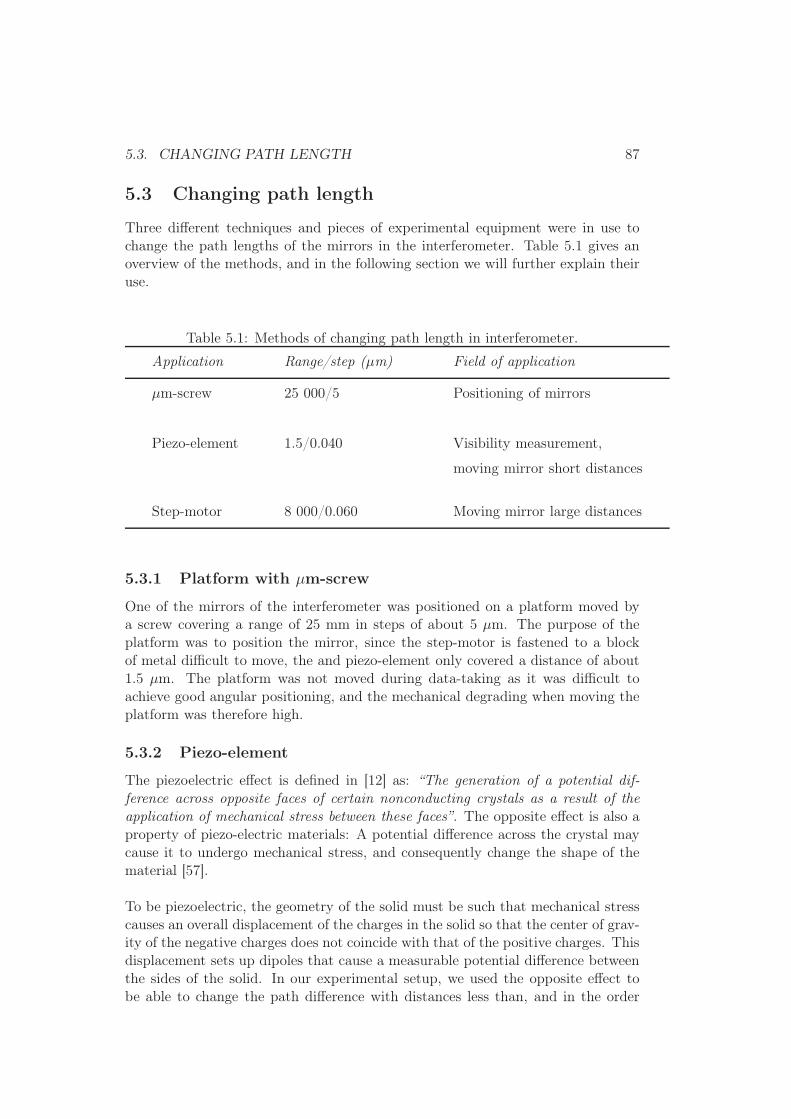
5.3. CHANGING PATH LENGTH 87
5.3 Changing path length
Three different techniques and pieces of experimental equipment were in use tochange the path lengths of the mirrors in the interferometer. Table 5.1 gives anoverview of the methods, and in the following section we will further explain theiruse.
Table 5.1: Methods of changing path length in interferometer.
Application Range/step (µm) Field of application
µm-screw 25 000/5 Positioning of mirrors
Piezo-element 1.5/0.040 Visibility measurement,
moving mirror short distances
Step-motor 8 000/0.060 Moving mirror large distances
5.3.1 Platform with µm-screw
One of the mirrors of the interferometer was positioned on a platform moved bya screw covering a range of 25 mm in steps of about 5 µm. The purpose of theplatform was to position the mirror, since the step-motor is fastened to a blockof metal difficult to move, the and piezo-element only covered a distance of about1.5 µm. The platform was not moved during data-taking as it was difficult toachieve good angular positioning, and the mechanical degrading when moving theplatform was therefore high.
5.3.2 Piezo-element
The piezoelectric effect is defined in [12] as: “The generation of a potential dif-ference across opposite faces of certain nonconducting crystals as a result of theapplication of mechanical stress between these faces”. The opposite effect is also aproperty of piezo-electric materials: A potential difference across the crystal maycause it to undergo mechanical stress, and consequently change the shape of thematerial [57].
To be piezoelectric, the geometry of the solid must be such that mechanical stresscauses an overall displacement of the charges in the solid so that the center of grav-ity of the negative charges does not coincide with that of the positive charges. Thisdisplacement sets up dipoles that cause a measurable potential difference betweenthe sides of the solid. In our experimental setup, we used the opposite effect tobe able to change the path difference with distances less than, and in the order

88 CHAPTER 5. EXPERIMENTAL SETUP AND METHODS
500 440 380 320−0.5
0
0.5
1
1.5
Voltage / V
Rel
ativ
e in
tens
ity
Figure 5.13: The piezo element glued to one of the mirrors enables us to change the path lengthwith distances in the order of one wavelength. The arrow to the far left and right on the x-axisshows that the voltage is kept constant at 500 V and 320 V respectively. The wavy or step-likefeature of the curve is due to an uneven rate of voltage change as described in the main text.
of one wave length: A varying potential difference between two of the sides of apiezoelectric crystal pulls the charges apart and gradually changes the size of thecrystal [51], [57].Figure 5.13 shows the intensity from the interferometer using a laser and changing
the voltage by turning a knob by hand. The step-like feature of the graph is due tothat hand work, as the author only managed to turn the knob about one half turnbefore having to take a new grip. Jagielski found in the work with his master’sthesis that the expansion of our piezo-crystal is linearly dependent on the voltageapplied [22].
5.3.3 Step-motor
To change the path length over a distance longer than approximately 1 µm dur-ing measurements, we used a combination of a Travel stepper actuator with anATP stepper motor controller, both from Thorlabs. The step-motor allows for pre-determining a sequence of moves to be carried out. In defining a move, the totaldistance, maximum speed, and acceleration must be defined.
As we will see below and in the next chapter, the step-motor was less stable andhad larger uncertainties than expected.
Uncertainty in linear distance
According to the description from the manufacturer, the actuator may cover a dis-tance up to 8 mm, with a minimum step size of 60 nm [49], and it should thereforebe possible to use the step motor for small changes in the path length. However, inexamining figure 5.14 and comparing the graphs obtained with the step-motor andthe piezo-element, it seems clear that the accuracy of the piezo-element is much
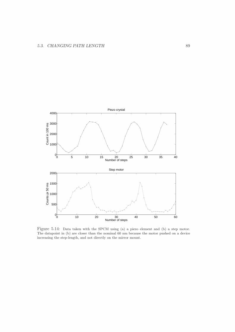
5.3. CHANGING PATH LENGTH 89
0 5 10 15 20 25 30 35 400
1000
2000
3000
4000
Number of steps
Cou
nt in
100
ms
Piezo crystal
0 10 20 30 40 50 600
500
1000
1500
2000
Cou
nts
pr 5
0 m
s
Number of steps
Step motor
Figure 5.14: Data taken with the SPCM using (a) a piezo element and (b) a step motor.The datapoint in (b) are closer than the nominal 60 nm because the motor pushed on a deviceincreasing the step-length, and not directly on the mirror mount.

90 CHAPTER 5. EXPERIMENTAL SETUP AND METHODS
larger than that of the step-motor, and correspondingly, the former was used dur-ing measurements.
Mechanical instability
4.25 4.3 4.35 4.4 4.45 4.5 4.55 4.6 4.65 4.7
0.2
0.4
0.6
0.8
1
time/sec
Inte
nsity
rela
tive
units
Figure 5.15: Tests with HeNe-laser and step-motor moving with a speed of 1 mm/10 sec.
During preliminary tests of the setup, we used a laser as light source, the Newportdetector described below as detection devise, and the step-motor, programmed tomove 1 mm in 10 sec to change the path length. The graph obtained is depictedin figure 5.15, and clearly shows an oscillating enveloping curve in addition to theexpected interference pattern. A priori, the oscillations could have four sources:
1. Instabilities in the laser
2. The limited temporal resolution of the detector
3. Mechanical instability of the step-motor
4. External noise.
To find the source of the oscillations, we measured the intensity as the step-motorwas moved with a speed of 1 mm/5 sec, 1 mm/10 sec, and 1 mm/20 sec. The datais plotted in figure 5.16.
Each of the three curves in figure 5.16 shows a segment of about 0.1 sec of the totaldata. In figure (a) one may see four periods of the oscillations, in figure (b) two,and in figure (c) only one oscillation. Temporally this corresponds to a period of0.025 sec, 0.05 sec and 0.1 sec, respectively.
Taking the speed of the motor, vmotor , into the calculation, the spatial period Ps ofthe oscillation is:
Ps = vmotor × Pt, (5.7)

5.3. CHANGING PATH LENGTH 91
5.41 5.42 5.43 5.44 5.45 5.46 5.47 5.48 5.49 5.50.4
0.5
0.6
0.7
0.8
time/sec
Inte
nsity
Rel
ativ
e un
its
4.46 4.48 4.5 4.52 4.54 4.56
0.4
0.6
0.8
1
time/sec
Inte
nsity
Rel
ativ
e un
its
3.28 3.3 3.32 3.34 3.36 3.38 3.40.02
0.04
0.06
0.08
0.1
time/sec
inte
nsity
rela
tive
units
Figure 5.16: Interference pattern of laser, with the step-motor used to change path length (a)1 mm in 5 seconds, (b) 1 mm in 10 seconds, and (c) 1 mm in 20 seconds.
where Pt is the temporal period of the oscillations.
Inserting the numbers for vmotor and Pt give above, we find that the spacial periodin all three cases is equal to 5µm. Since the oscillations seem to have a fixedspacial, and not temporal period, we concluded that they are due to mechanicalinstabilities of the step-motor.
Let us examine the graph in figure 5.16 once more. The maximum and minimumvalues of the oscillations change, but the shape of each top does not seem to besignificantly disorted. If the latter had been the case, it would have been an indic-ation that the speed of the stepmotor is not constant. Instead, we have a periodicchange of the value of the maxima and minima of the curve, and consequently ofthe visibility. We already showed that the periodicity of the envelope is causedby instabilities in the mechanics of the step-motor. It therefore seems natural to

92 CHAPTER 5. EXPERIMENTAL SETUP AND METHODS
conclude that in the forward motion of the mirror, there is a slight angular rockingof the mount of its mount.

5.4. DETECTORS 93
5.4 Detectors
Several means of light detection were used during the experimental work: A singlephoton counting module (SPCM) from PerkinElmer, a silicon photodetector (SPD)from Newport, and a USBeamPro beam profiler from Photon Inc. Following theprocedure of the section on methods of changing arm length, brief information onthe use of each detector is given in table 5.2, followed by a section of a descriptionof each. The SPD and the USBeamPro will be treated very briefly, the SPCM thatwere used during the actual measurements in some more detail. The data obtainedfrom the SPD and the SPCM were analysed using a LeCroy digital oscilloscope.A brief description of this is given after the descriptions of the detectors. Sincedescriptions of all three detectors are readily available online, our focus will be ongiving subjective discussion of our experience of the strengths and weaknesses ofeach module.
Table 5.2: Detectors and their use.
Detector Field of application
SPCM Numerical intensity measurement of
intensities on the single-photon level
SPD Numerical intensity measurement for
low to moderate intensities
USBeamPro Visualizing the beam,
determining beam shape and size
5.4.1 USBeamPro
The colorful images in 5.8 were made using the USBeamPro beam profiler fromPhoton Inc. The detection device consists of a camera-based CMOS-chip7 with1280×1024 pixels, each of size 6.7 × 6.7 µm, giving a total active area of 8.6 ×6.9 mm. The spectral range of the device is 360 nm - 1100 nm [37]. The camerais directly connected via an USB-cabel to a computer, where the data is analysedwith software following the camera. An example of the graphical interface and thepossibilities of the program of analysis is shown in figure 5.17.
7CMOS: Complementary metal oxide semiconductor, similar to the CCD decribed onpage 75. In a CMOS, each pixel has its own output-node, allowing for large variety in thefunctioning of the chip, but with lower uniformity than for the CCD [13].

94 CHAPTER 5. EXPERIMENTAL SETUP AND METHODS
Figure 5.17: Anomg the possibility of the analysis of data obtainded with the USBeamPro are:Color coded intensity distribution in 2D and 3D, time evolution of the beam width, numericaldata and gaussian fit of the intensity distribution.
5.4.2 Silicon photodetector (SPD) and power meter
While testing the experimental setup with the HeNe-laser, we combined a siliconphotodetector(SPD) and a power-meter from Newport. The spectral range of thedetector was 400-1100 nm [30]. The combination was not possible to use duringmeasurements on the spectral lamps for reasons described below.
Sensitivity
According to the description from the manufacturer, the detector is sensitive tointensities down to the pW-level. On that level, however, the signal-to-noise ratiowas far below a level where we could do measurements on the spectral lamps.Figure 5.18 shows the interference pattern close to ∆l = 0 for the unfiltered neonlamp. The gray signal show the original signal, while the black line is the smootheddata. Experiments showed that filtering out the Ne692-line would decrease theintensity with a factor 40, and with an intensity that low, it would not be possibleto distinguish the signal from the noise, at least not to the level we would need tomake a good determination of the visibility of the signal.

5.4. DETECTORS 95
Figure 5.18: Interference of a neon lamp at ∆l = 0. The gray area show the original data, toobtain the black line we have used the smooth-function described in chapter 3.
2 4 6 8 100.12
0.125
0.13
0.135
0.14
0.145
time / sec
Inte
nsity
(o
scill
osco
pe o
utpu
t / V
)
Figure 5.19: Pulsating signal due to limited temporal resolution of the SPD. The gray area isthe original signal, the black line a smoothing over 50 datapoints, using the smooth-function.

96 CHAPTER 5. EXPERIMENTAL SETUP AND METHODS
Temporal resolution
The sensitivity of the detector was highly dependent on its temporal resolution,and using the power meter setting to obtain the highest possible sensitivity meanthaving the sampling rate in the order of 1 Hz. As a result, the signal showed thepulsating behaviour depicted in figure 5.19. A signal that is already weak could besignificantly disorted by the pulsations. Also, to calculate the visibility of a signal,accurate values for the maximum and minimum points of a graphs is required.
5.4.3 Single photon counting module (SPCM)
General description
0 1 2 3 4 5 6 7 8
0
2
4
6
Time / 10−3sec
Vol
tage
/ V
0 5 10 15 20
0
2
4
6
Time / 10−9sec
Vol
tage
/ V
Figure 5.20: Output signal from the SPCM. Upper frame: The total signal. Lower frame: Thetemporal width of a single pulse.
To detect light with very low intensities, we used a Single photon counting modulefrom PerkinElmer. An example of its output data is shown in figure 5.20.
The name of the module and the appearance of its output favor a picture of eachpulse detected corresponding to a quantum of light as it was briefly described inthe introduction to chapter 1. In any detector, the detection process involves aninteraction between electromagnetic radiation and a charged particle [27]. In ouropinion, the implied assumption that a pulse in figure 5.20 must correspond tothe indivisible particle we normally have in mind when the word photon is used,

5.4. DETECTORS 97
therefore seems somewhat hasty.
The active part of the spcm is a circular silicon avalanche photodiode with anactive area of diameter of 180 µm [36]. The detection efficiency for light of a givenfrequency is given in figure 5.21. The output rate was found using a simple Matlabroutine, that counted the number of pulses while taking into account the temporalwidth of a single pulse as shown in the upper frame in figure 5.20. The code couldbe run directly on the oscilloscope to avoid having to store large quantities of data.
According to the data sheet from the manufacturer [36], the actual photon ratecompared to the output rate is
ACTUAL =(OUTPUT × CORRECTION FACTOR) − DARK COUNT
PHOTON DETECTION EFFICIENCY.
The correction factor is a factor dependent on the count rate, that takes the de-tector dead time8 into account. Its value as a function of rate is shown in figure 5.21.For count rates smaller than about one million, it is very nearly equal to unity. Asexplained below, we never exceeded 40 000 counts/sec in our experiments, and thecorrection factor was therefore neglected in our calculations. The inverse factor ofthe photon detection efficiency has been neglected since it cancels out in the calcu-lation of visibility. The detection efficiency did however, as we argued in chapter 4,play a part in our choice of light sources.
Degrading, and dark count rate
According to the detector manual, the SPCM should manage a count rate ex-ceeding 20 million counts per second [36], but according to the experience of theexperimental quantum optics group of the Bohr Institute at the University ofCopenhagen, the module is permanently degraded if the count rate over time ex-ceeds 40 000 counts/sec [53].
The nominal maximum dark count rate of our module is 25 counts/sec, but approx-imately one year after the purchase, it was measured to be 800 ± 100 counts/secand 150 ± 50 counts/sec respectively for two of our detectors [22]. Some monthslater, we measured the dark count to be 800±100 counts/sec and 900±100 count-s/sec. During the measurements, the photodiode was covered with a black rubbercap of thickness about 2 mm, and the whole detector was covered by a black boxof thickness about 5 mm. To our knowledge, the detectors have not been subjectto intensities above approximately 40 000 counts/second.
5.4.4 LeCroy digital oscilloscope
As mentioned above, the data from the SPD and SPCM were displayed usinga computer based oscilloscope from LeCroy. The oscilloscope has a maximum
8Dead time: The time from a pulse is registered till the detector is ready to detect the nextpulse.
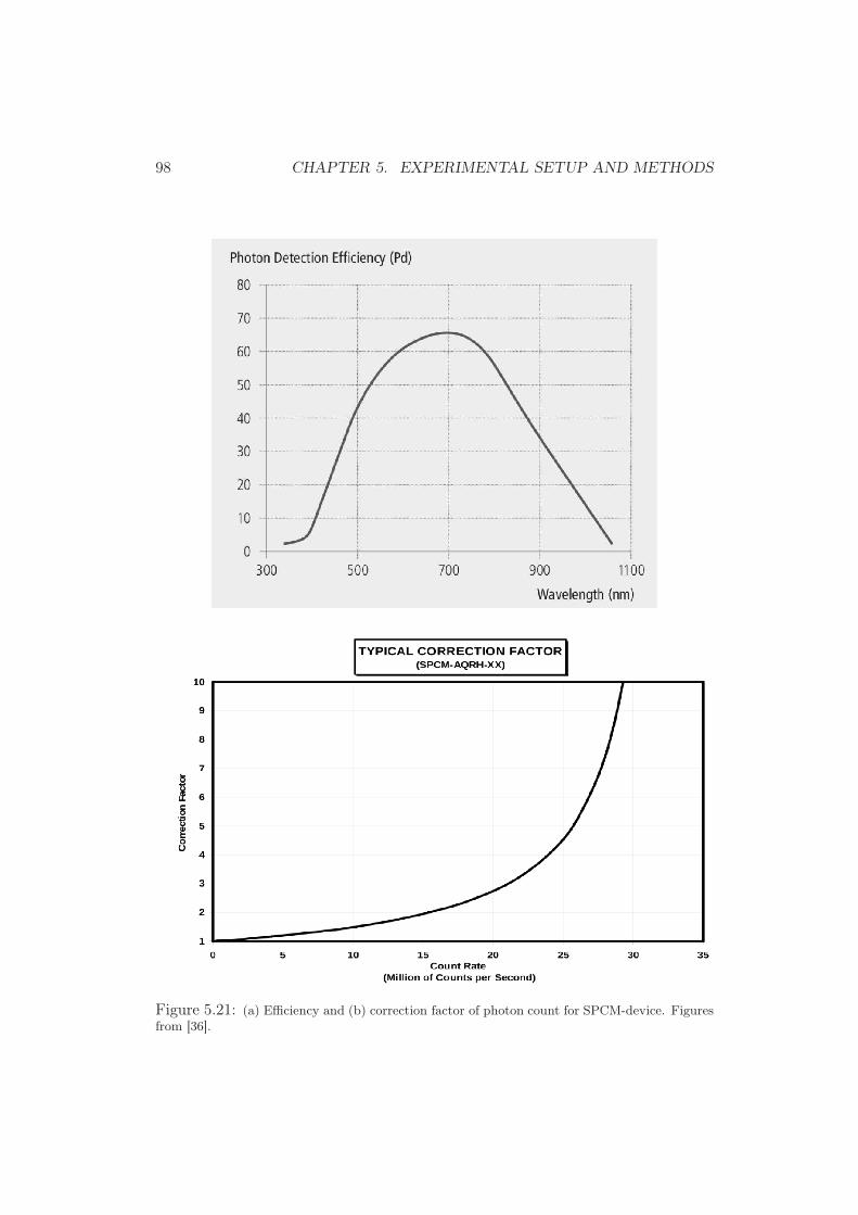
98 CHAPTER 5. EXPERIMENTAL SETUP AND METHODS
Figure 5.21: (a) Efficiency and (b) correction factor of photon count for SPCM-device. Figuresfrom [36].

5.4. DETECTORS 99
temporal resolution of one datapoint per 50 psec. The oscilloscope settings had tobe chosen to fulfill the following criteria:
• To make sure the temporal resolution is high enought for all pulses to bedetected, each pulse had to be at least two datapoints long
• The time span of one measurement should be as long as possible to obtainhigh statistics and even out possible fluctuation in the background and in-tensity of the beam
• The dataset should be of manageble size to minimize processing time
We found that for our use, a time span of 100 µsec and a total datalength of10 Mega-samples was a good compromize. This gives a temporal resolution of10 nsec per datapoint.
At the closing, let us mention one detail that may save a future user for frustrationand waste of time. A bug in the software included in the oscilloscope causes thecomputer to crash if one tries to overwrite a file. All filenames must therefore bechanged before saving.
5.4.5 Time-digitizer
Towards the finish of the experimental work, the laboratory was granted the eco-nomical means necessary to purchase a time-digitizer. The most important facetof a time-digitizer is that it may record the syncronized time of hits from differentdetectors. No selection of data needs to be made during measurements, and notrigger-mechanism between the two detectors are needed. In addition, only thetime for registered hits are recorded. This significantly decreases the size of thedata-sets that have to be saved and processed [53]. It is possible that the experi-ments described in this thesis could be done more easily and accurately with thisnew device.

100 CHAPTER 5. EXPERIMENTAL SETUP AND METHODS
Table 5.3: Reference data of experimental equipment.
Name Product code Manufacturer
HeNe-laser HRR120 Thorlabs
Broadband dielectric mirror BB1-E02 Thorlabs
Beam splitter TWK 10 Bernhard Halle
Plano-convex lens KPX100 Newport
Spectral calibration lamp 6030 Argon Newport/Oriel
Spectral calibration lamp 6032 Neon Newport/Oriel
Spectral calibration lamp 6035 Mercury (Argon) Newport/Oriel
Bandpass filter (mercury) 546FS05-25 Andover
Bandpass filter (neon) 690FS10-25 Andover
Bandpass filter (argon) 694FS10-25 Andover
Single mode fiber P1-630A-FC-10 Thorlabs(neon, argon)
Single mode polarizing P1-488PM-FC-5 Thorlabsmaintaining fiber (mercury)
Single mode fiber launch MBT613/M Thorlabs
Microscope objective RMS20X Thorlabs/Olympus
Travel stepper actuator DRV001 Thorlabs
ATP stepper motor controller BSC102 Thorlabs
Single Photon SPCM-AQRH-16 PerkinElmerCounting Module
USBeamPro PS-2323 Photon Inc.
Silicon photodetector 918D-SL-OD3 Newport
Power Meter 2931-C Newport
LeCroy Digital Oscilloscope WP7100A LeCroy

Chapter 6
Experimental results for Ne692
We will now present the experimental results for Ne692. Some data was alsoobtained from Hg546. As we will see, an accurate measurement of the laser visib-ility was required to allow any conclusions from the measurements of the spectrallamps. Measurements of the laser visibility was only done during the experimentson Ne692. Attempts to use the same values for Hg546 were unsuccessful, and theresults for this will therefore not be included in the chapter.
During the measurement on Ne692, it became clear that the limitations on theequipment did not allow us to obtain the results with the accuracy first expected,and we therefore chose not to spend time on repeating the measurements for Ar696.
The average background (including dark counts) was found to be about 110 countsper 100 µsec.
6.1 Measurements
We used the experimental setup depicted in figure 5.6. A SPCM was used as detec-tion devise, and the intensity was assumed to be proportional to the pulse-densityafter the background had been subtracted. A simple Matlab-routine was used tocount the number of pulses.
The total measurement consisted of several sets of sub-data, each data-set corres-ponding to intensity measurement over a distance of 2-3 wavelengths. To changethe path length within one set of sub-data, a piezo-element was used. Linearitybetween the voltage applied and distance was assumed (cf. discussion of the piezo-element in chapter 5). Between each set of sub-data, the step-motor was moved1 mm, corresponding to a total path difference of ∆l = 2 mm.
Figure 6.1(a) shows the intensity of Ne692 as a function of path difference in theinterferometer. In figure 6.1(b), we have zoomed in on the set of sub-data at∆l = 0. Note that the units of the x axis in the first case is in millimeters, in the
101

102 CHAPTER 6. EXPERIMENTAL RESULTS FOR NE692
0 4 8 12 16 20 24 28 320
1000
2000
3000
∆l / mm
Cou
nts
per
100µ
sec
320 345 370 395 420 445 470 495 5200
1000
2000
3000
Voltage / V
Cou
nts
per
100µ
sec
Figure 6.1: (a) The visibility of Ne692 as function of path difference, and (b) the intensity ofNe692 zoomed in on the sub-data at ∆l = 0 mm (the far left line of data-points in the uppergraph).
second case in volts to reflect the method used for moving the mirror.
For values of ∆l from 0 mm to 18 mm, the measurements were made in orderof increasing ∆l (0 mm, 2 mm, 4 mm, ..., 16 mm). The µm-platform was thenmoved to give a total path-difference of 30 mm. As we will see below, movingthe step-motor caused a large mechanical degrading of the visibility. The mirrorswere therefore re-adjusted to obtain the highest possible visibility for the laser.Measurements were then made for decreasing values of ∆l (30 mm, 28 mm, ...,18 mm).
6.2 Discarding data
6.2.1 Discarding the data for ∆l = 30 mm
In figure 6.1, the set of data for ∆l = 30 mm does not seem to stand out amongthe other sets; its maximum and minimum values are about the same as for theprevious data-sets, and the data-points seem to be evenly distributed as for the

6.2. DISCARDING DATA 103
320 345 370 395 420 445 470 495500
1000
1500
2000
2500
3000
Voltage / V
Cou
nts
per
100µ
sec
Figure 6.2: The data at ∆l = 30 mm.
rest of the sets. When we zoom in on the set, the situation is another. As shownin figure 6.2, there is no indication of the data-points forming a function similarto the form of a sine.
We did not arrive at finding the reason for the strongly oscillating pattern in thefigure. I could be an indication that we are past the coherence length, but asshown in figure 6.4 and in the data in appendix B, the visibility at ∆l = 28 mmwas about 0.6, and having no sign of an interference pattern at 30 mm thereforeseems unlikely. In addition, an integration period of 100 µm is very long comparedto the time it takes the light to move a distance of one wavelength. According tothe theory discussed in chapter 2, with ∆l >> lcoh one would expect a constantintensity equal to half the incoming intensity of the light, something that is hardlythe case in figure 6.2.
As mentioned in the beginning of the chapter, the data-set obtained for Hg546is incomplete, and we do not have any data for Ar696. In the lack of a possibleexplanation or other measurements confirming the results presented in figure 6.2we decided to discard the data-set in the determination of the visibility of Ne692.
6.2.2 Discarding of data due to hysteresis of piezo-element
Examine figure 6.3 showing the sets of sub-data for ∆l = 2 mm and ∆l = 6 mm.The right hand side of the figures resemble nicely periodic sines, while the left sideof the figures do not. All sets of sub-data showed the same behaviour, except forthe data for ∆l = 0 mm (cf. figure 6.1(b)). Recall that this was the first set ofdata to be recorded. Starting from the second set of sub-data, the voltage over thepiezo-element was turned from 520 V to 320 V immediately before beginning themeasurements, and the left-most data point were the first to be recorded in eachdata-set. We therefore believe the unpredictability of the first part of the data-setto be due to hysteresis of the element.

104 CHAPTER 6. EXPERIMENTAL RESULTS FOR NE692
320 345 370 395 420 445 470 495 5200
1000
2000
3000
Voltage / V
Cou
nts
per
100µ
sec
320 345 370 395 420 445 470 495 5200
1000
2000
3000
Voltage / V
Cou
nts
per
100µ
sec
Figure 6.3: The data for (a) ∆l = 2 mm and for (b) ∆l = 6 mm.
Data-points that seemed to have been subject to this hysteresis were not includedin the least-square fit described above.
6.3 Finding the visibility of the spectral lamps
To determine the coherence length, we needed to find the visibility of the datapresented in figure 6.1. Since the measurements clearly show an interference pat-tern for path differences of more than one centimeter, the visibility within one setof sub-data may be taken to be constant. To find the visibility of each set of sub-data, we made a least-square fit to a sine as indicated in figure 6.1. The visibilityof the data set was then defined as the visibility of the cosine. The sets of sub-dataand the code used to find the least-square sine fit are included in appendix B.

6.3. FINDING THE VISIBILITY OF THE SPECTRAL LAMPS 105
Scaling factor from laser visibility
The visibility of the laser was measured to be1
V (0 mm) = 0.921
V (16 mm) = 0.744 ± 0.002
After the path-difference had been changed to 30 mm and the mirrors re-adjusted,we measured a visibility of:
V (30 mm) = 0.954 ± 0.002
V (18 mm) = 0.719 ± 0.004
At ∆l = 16, 18 and 30 mm, two measurements of the visibility of laser were madefor each value of the path difference. The uncertainty of the numbers only reflectthe spread of the two measurements. The uncertainty due to varying backgroundis probably somewhat higher.
The fact that the visibility of the laser was ∼ 0.2 larger for a path difference of30 mm than at 16 mm is a clear sign that in moving the step motor, there is a sig-nificant mechanical degrading of visibility (cf. discussion on page 82). To accountfor this fact when finding the visibility of the spectral lamps, we scaled each of themeasurements with the visibility of the laser. In lack of accurate measurements ofthe laser visibility at each data-point, we assumed linearity.
In our simple scaling, we implicitly assumed that the degrading of the laser visib-ility was solely due to the mechanical degrading of the system, not to the limitedcoherence length of the laser itself. For this assumption to be valid, the coherencelength of the laser must be much longer than the maximum path-difference in themeasurements. The coherence length of the HeNe-laser used in the adjustmentswere in the order of 18 cm [22].
Calculation of visibility for Ne692
In chapter 4, we showed that spectral lines dominated by homogeneous and in-homogeneous broadening produced an exponential and Gaussian visibility functionrespectively. In figure 6.4 we have plotted the measured and scaled data with bothan exponential and a Gaussian fit. Both functions were found using the built inMatlab-routine cftool of the scaled data.
The Gaussian curve reaches the value e−1 when ∆l = 33.8 mm, the exponentialwhen ∆l = 27.1 mm. Since a physical light source in general is somewhere betweena pure Gaussian and a pure Lorentzian, it seems natural to conclude that the
1The laser visibility was actually not measured at ∆l = 0 mm. The visibility mentionedbelow is the visibility found from the data of Ne692.

106 CHAPTER 6. EXPERIMENTAL RESULTS FOR NE692
0 10 20 300
0.2
0.4
0.6
0.8
1
∆ l / mm
Vis
ibili
ty
Measured dataScaled dataexp{−(∆ l/16.9)2}
0 10 20 300
0.2
0.4
0.6
0.8
1
∆ l / mm
Vis
ibili
ty
Measured dataScaled dataexp{−0.037∆ l}
0 10 20 30 40 50 60 70 80 90 1000
0.2
0.4
0.6
0.8
1
∆ l / mm
Vis
ibili
ty
Figure 6.4: The visibility of Ne692 as function of path difference. (a) Measured and scaledvisibility with a Gaussian fit. (b) Scaled visibility and Gaussian fit, showing the expected totalvisibility function. The figures (c) and (d) show exponential fit,

6.4. PULSE NUMBER-DENSITY 107
coherence length of Ne692 most likely lies in the interval:
27.1 mm < lcoh(Ne692) < 33.8 mm, (6.1)
where the value ∆l = 27.1 mm corresponds to a purely Lorenzian source, and∆l = 33.8 mm to one that is purely Gaussian.
6.4 Pulse number-density
The average distance between two pulses is given by the number of pulses per unittime divided by the speed of light. In our case, the maximum pulse number densityn was about 3 200 per 100 µsec, which gives 32 000/sec. From figure 5.21, we findthat the detection efficiency at wavelengths around 700 nm is about 65%, so theactual number density is in the order of 49 000/sec. The refracive index of air isvery close to unity (see footnote on page 65), so the speed of light in air is veryclose to the speed of light in vacuum, about 3.0×10⁸ m/sec. The average distancebetween two pulses is then:
3.0 × 10⁸ m/sec
4.9 × 10⁴ pulses/sec= 6 × 10³ m/pulse.
The length of one arm of our interferometer was in the order of 10 cm, much shorterthan the average distance of 6 000 meters between each pulse.
It should be mentioned that in our simple calculation above, we have not con-sidered the statistical distribution of the light pulses. In general, for thermal light,this will be Poisson distributed. A distance of 6 000 meters between two pulsesis nevertheless large enough to assume that two pulses were never present in theinterferometer at the same time, and consequently our experiments may be saidto have been carried out at the single-photon level. In addition to being simplya measurement of the coherence length of a spectral line, we have with the abovedescribed experiment and results made a demonstration of one of the puzzelingascpects of the wave-particle duality mentioned in the introduction and at thebeginning of chapter 1: Even though some experiments seem to require a descrip-tion of light as an indivisible particle, light of intensities that indicate that we areworking with only one particle at a time also show their wave-behavior throughinterference.

108 CHAPTER 6. EXPERIMENTAL RESULTS FOR NE692

Chapter 7
Summary and outlook
As a finish, we will give a brief summary of our treatment of the concept of coher-ence and of our experimental work. We will then round off with some suggestionsfor future work, and some concluding remarks.
Coherence summarized
During the work, we have encountered several ways of representing or picturingtemporal coherence of light. Coherence has been related to the size of a photon,to the average time between fluctuations in an electric field, and to the width ofthe auto-correlation function and of the power spectral density. The two formermay be said to be of more phenomenological nature, the two latter more formal.
Temporal coherence length lcoh = cτ was defined in chapter 2 to be the length equi-valent to the time-difference τ where the auto-correlation function has a value ofe−1. In the same chapter, we proved analytically that with this definition, the de-gree of first-order coherence may be found through sending light through a Michel-son’s interferometer, and finding the visibility as a function of path length. Wealso showed that defining the coherence length using the first-order auto-correlationfunction as above is equivalent to using the width of the power spectral density, asthe two make up a Fourier-pair. The relations between the first-order correlationfunction, visibility, and power spectral density were illustrated using numericalsimulations in chapter 3.
In defining coherence length using the auto-correlation function, we impute restric-tions on the other suggested ways of perceiving coherence. The phenomenologicalpictures are only valid to the extend they correspond to the definition. By usinga pulse-model, our simulations showed that coherence length may only correspondto photon size if one is willing to abandon the picture of a photon being the ori-ginal pulse, and instead use the term to denote the wave packets that arise as acollective effect when one superposes several pulses.
The image of coherence length as equivalent to the average time between fluctu-
109

110 CHAPTER 7. SUMMARY AND OUTLOOK
ations has not been expressly treated. In assembling bits and pieces from several ofthe chapters, we may, however, argue that though it may not in itself be identifiedas the coherence length, it may nevertheless be an important factor of limiting thecoherence length of a given light source.
As mentioned above, we have shown that defining coherence length using the widthof the auto-correlation function is equivalent to defining it using the power spec-tral density. The theory developed in chapter 2 says nothing explicitly about thefluctuations. Light made up of a large number of perfect lasers, each with infinitecoherence length but slightly different wavelengths would, according to the theory,still have a finite coherence length since its spectrum would not be infinitely thin.
On the other hand, as we saw in chapter 2, power spectral density is equal to theabsolute square of the frequency distribution of the electric field. A wide frequencydistribution would cause the power spectral density to also be wide. Random fluc-tuations of the electric field may be defined as random deviations from the shapeof a perfect cosine1. As it is shown in our presentation of the mathematics ofFourier transforms in appendix A, a large deviation from a cosine will result inmore components in the Fourier spectrum2. Deviations, discrete or continuous,from a pure cosine, will therefore serve to broaden the spectrum and therefore alsothe power spectral density, and the coherence length will shorten.
In the description of broadening mechanisms in chapter 4, we argued that “Eachtime an excited atom undergoes a collision, it may gain or lose energy. The totaltransition rate will therefore be higher than the rate one gets from Heisenberg un-certainty relation only”. A collision may be imagined to cause an abrupt changein the electric field. Collision broadening may therefore be seen as one physicalexample of how the coherence length may be altered from deviations from thecosine-shaped electric field.
Albeit perhaps superfluous, we would like to again stress that a finite coherencelength does not necessarily mean that those random fluctuations take place. Tofind a physical example of this, one needs only to again look at the discussionof Doppler broadening following that of collision broadening. It should also bepointed out that a collection of light sources (with infinite coherence length) ofdifferent velocity distributions is mathematically equivalent to the collection ofperfect lasers mentioned above.
1Or sine.2As implied from the discussion in appendix A, and from table A.1 in particular, the extreme
example of deviation from a pure cosine is the δ-function. The Fourier transform of the δ-functionis a constant line, so to write the δ-function as a sum of cosines, all frequencies are needed, thespectrum is infinitely broad, and the coherence length infinitely small.

111
Experimental work: Experience gained
The experiments proved to be technically harder and more time-consuming thanexpected, and some of the components of the setup offered negative surprises intheir stability and resolution. As described in the previous chapter, we did man-age to show interference of Ne962 at the single-photon level, and the visibilitywas decreasing more than what may be accounted for from a purely mechanicaldegrading. The coherence length of the spectral line seems to be in the order of afew centimeters.
The most important value of the experimental work that has been done, is per-haps the work described in chapter 5, where the experimental applications havebeen analysed. During the year that has passed since the work started, we havegained knowledge on the whims of the equipment, and methods passed on fromthe experiences of others have been tested and modified for our use.
Work yet to be done: Future perspectives
As the time reserved for the work approaches the end, the author has the strongimpression that more questions have been posed than answered. Some of thosequestions could, perhaps, be explored in the work of another student:
1. Theory and numerical simulation
• Is it possible to use statistical physics to analyse the features of the auto-correlation function? How does the auto-correlation function dependon the parameters of the emission model employed, and what may thatteach us about nature?
• What would the figures 3.9 and 3.10 look like if the original pulse didnot have a Gaussian envelope, and especially if it were not symmetric?
2. Experiment
• If the measurements on Ne692 are repeated, are the large fluctuationsat ∆l = 30 mm reproduced? If the fluctuations are found, do Hg546and Ar696 show the same behavior? What about other light sources?
• Do the coherence length and the shape of the auto-correlation functiondepend on the intensity of the beam, as our simulations suggest?
• Is it possible to obtain more accurate data using a time-digitizer ratherthan an oscilloscope?
Concluding remarks
As defined in the introduction, the goal of this work was originally to obtain agreater understanding of the concept of coherence, through experimental measure-ments of the coherence length of atomic spectral lines. If judged by the experi-mental results alone, the work can hardly be said to have been as successful as
112 CHAPTER 7. SUMMARY AND OUTLOOK
we were hoping for. It is the author’s hope that the experimental work may becontinued by another student. In that case, a year of struggling in the dark3 is ayear of experience gained, and may be said to have been a necessity.
If judged by the criteria of having increased our understanding of coherence, thepicture seems to be quite different. We would especially like to mention again thenumerical analysis in chapter 3. The simulations, which originally were planned toillustrate the theorems and relations found in chapter 2, showed some surprisingdetails that could open the way for an experimental determination of the natureand shape of the light emitted from atoms.
3Literally!

Appendix A
Fourier transforms
Since Fourier transforms have been used in several places in the thesis, we hereinclude a very brief introduction to the idea behind the mathematics. The fo-cus has been on making the main idea conceptional clear. Mathematical proofsand theorems may be found in basically any book on mathematical methods forscientists, we used [4] and [41].
A.1 General introduction
Let us begin this section with an example taken from J. F. James’ little book [24],which well describes the idea of Fourier transforms.
Imagine singing a steady note, where the air pressure F as a function of time canbe described as a pure cosine1 (the factor 2A is just a constant):
F (t) = 2A cos (2πν0t). (A.1)
Alternatively, this can be rewritten using Euler’s formula2:
F (t) = A(e+i2πν0t + e−i2πν0t). (A.2)
A note sung is rarely a pure cosine. If one is trying to sing the note La, the maincontributor will be a pressure function of frequency 440 Hz, but other frequencieswill play a part, giving the voice its particular flavor. The resulting signal maylook like the graph in figure A.1. To better visualize the frequency contents of asignal, one may instead choose to plot the amplitude in front of each exponential,as a function of the frequency. The graph may then look like figure A.2. However,
1Although more common to define an ω = 2πν, I am choosing to follow the conventionof James [24] for two reasons: It avoids the somewhat awkward factors of 1√
2πin front of the
Fourier integrals, and it avoids having to introduce -for our use- the more abstract idea of angularfrequency, making the transition to frequency spectra of light very straight-forward.
2Euler’s formula says that eix = cosx + i sin x. Using it with the identities of the trigo-nometric functions: sin (−x) = − sin x and cos (−x) = cos x one may deduce the formula for thecosine: cos x = (eix + e−ix)/2.
113

114 APPENDIX A. FOURIER TRANSFORMS
0 0.005 0.01 0.015 0.02 0.025 0.03 0.035 0.04 0.045 0.05
−1
0
1
2
Time / s
Rel
ativ
e pr
essu
re
Figure A.1: The signal coming from a voice more flavorful than one that holds a pure cosine.
Figure A.2: The frequency spectrum of the pressure function of the flavorful voice in figure A.1(We have omitted the negative frequencies since, according to equation (A.2) this would be themirror-image of what we show).
in gaining information about the frequency content, we lose information of thetime-aspect and phase of the original function.
In general, a signal that consists of a sum of cosines may be written using the form
F (t) = A(ν0)ei2πν0t +A(ν1)e
i2πν1t +A(ν2)ei2πν2t + ...+A(νn)ei2πνnt
=
n∑
m=0
A(νm)ei2πνmt.(A.3)
To describe a function very different from a cosine, one may need the entire con-tinuous set of frequencies, and the sum in equation (A.3) becomes an integral3
F (t) =
∫ ∞
−∞A(ν)ei2πνtdν.
If we know the function A(νm), the function F(t) is unambiguously determined.A(ν) is called the Fourier transform of F(t). It can be shown that F(t) is alsothe Fourier-transform of A(ν), provided that one multiplies the exponent by a
3It may not be obvious that any function may be written as a sum of harmonic functions. Itmay however be shown that this is the case for most well-behaved functions [41].
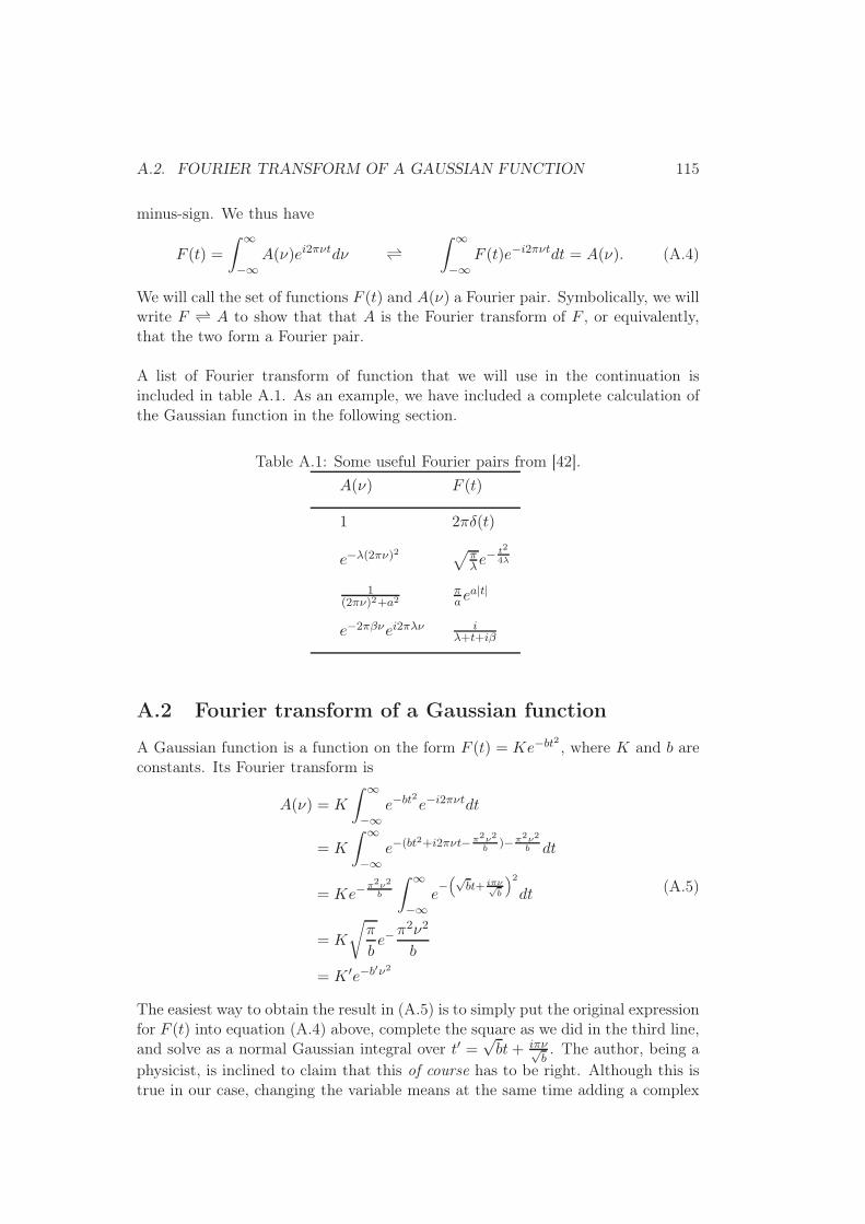
A.2. FOURIER TRANSFORM OF A GAUSSIAN FUNCTION 115
minus-sign. We thus have
F (t) =
∫ ∞
−∞A(ν)ei2πνtdν ⇀↽
∫ ∞
−∞F (t)e−i2πνtdt = A(ν). (A.4)
We will call the set of functions F (t) and A(ν) a Fourier pair. Symbolically, we willwrite F ⇀↽ A to show that that A is the Fourier transform of F , or equivalently,that the two form a Fourier pair.
A list of Fourier transform of function that we will use in the continuation isincluded in table A.1. As an example, we have included a complete calculation ofthe Gaussian function in the following section.
Table A.1: Some useful Fourier pairs from [42].
A(ν) F (t)
1 2πδ(t)
e−λ(2πν)2√
πλe
− t2
4λ
1(2πν)2+a2
πae
a|t|
e−2πβνei2πλν iλ+t+iβ
A.2 Fourier transform of a Gaussian function
A Gaussian function is a function on the form F (t) = Ke−bt2 , where K and b areconstants. Its Fourier transform is
A(ν) = K
∫ ∞
−∞e−bt2e−i2πνtdt
= K
∫ ∞
−∞e−(bt2+i2πνt−π2ν2
b)−π2ν2
b dt
= Ke−π2ν2
b
∫ ∞
−∞e−
“√bt+ iπν√
b
”2
dt
= K
√
π
be−π2ν2
b
= K ′e−b′ν2
(A.5)
The easiest way to obtain the result in (A.5) is to simply put the original expressionfor F (t) into equation (A.4) above, complete the square as we did in the third line,and solve as a normal Gaussian integral over t′ =
√bt+ iπν√
b. The author, being a
physicist, is inclined to claim that this of course has to be right. Although this istrue in our case, changing the variable means at the same time adding a complex

116 APPENDIX A. FOURIER TRANSFORMS
Figure A.3: The loop over which the integral is done.
factor to the integration limits, and it is in general a problem to have complexlimits of an integral over a real variable. To make our claim more plausible, onecan argue that in an integral on the form
∫ ∞
−∞e−bt2e−i2πνtdt (A.6)
the function ebt2
goes so fast to zero that the oscillations caused by the imaginaryterm don’t contribute enough to make the infinities a problem. However, to bemathematically rigid one should use Cauchy’s theorem4 on the rectangle C in thecomplex plane that has its corners in the points ±R and ±R−iπν/b. Se figure A.3.
Making the shift z = t− iπν/b, one has
A(ν) =
∫ ∞− iπνb
−∞− iπνb
e−bz2dz (A.7)
Since e−bz2is analytic everywhere, we have
∮
Ce−bz2
dz =
∫ R
−Re−bz2
dz+
∫ R− iπνb
Re−bz2
dz+
∫ −R− iπνb
R− iπνb
e−bz2dz+
∫ −R
−R− iπνb
e−bz2dz = 0
(A.8)In the limit R→ ∞, the first integral in (A.8) is just the normal Gaussian integralthat can be looked up anywhere (for example in [42]), and that equals
√
π/b. If theintegration limits are interchanged, the third integral is the same as our integralfor A(ν) in equation (A.7). Shifting the integration variable (and limits) of the
4Cauchy’s theorem: The loop integral of an area in the complex plane, with no singularities,is equal to zero [4].

A.2. FOURIER TRANSFORM OF A GAUSSIAN FUNCTION 117
second integral to z → z + iπν/b and making the substitution z′ = −z, it is fairlyeasy to see that this integral cancels the fourth, and we are left with
[
√
πb −
∫ R− iπνb
−R− iπνb
e−bz2dz.
]
R→∞= 0 (A.9)
Taking the limit R→ ∞ should convince the reader that (A.5) is correct [4], [38].
In any case, A(ν) is also Gaussian, but with new constants K ′ = K√
π/b andb′ = π2/b. Therefore, the narrower the original Gaussian is, the broader its Fourierpartner.
−2 −1 0 1 20
0.5
1
1.5
frequency /s−1
Am
plitu
de
−2 −1 0 1 20
0.5
1
1.5
time /s
ampl
itude
Figure A.4: The Fourier transform of a Gaussian function is also Gaussian. The lower andwider the original graph, the narrower and higher is its Fourier partner (In the above figures,K = b = 1).

118 APPENDIX A. FOURIER TRANSFORMS

Appendix B
DataFor reference we will here include the graphs of the original data of the intensityof of Ne692. The whole gray line is a least-square fit of a sine found using the codein section B.2.
B.1 Data
320 345 370 395 420 445 470 495 5200
1000
2000
3000
Voltage / V
Cou
nts
per
100µ
sec
0 mm
320 345 370 395 420 445 470 495 5200
1000
2000
3000
Voltage / V
Cou
nts
per
100µ
sec
2 mm
320 345 370 395 420 445 470 495 5200
1000
2000
3000
Voltage / V
Cou
nts
per
100µ
sec
4 mm
119

120 APPENDIX B. DATA
320 345 370 395 420 445 470 495 5200
1000
2000
3000
Voltage / V
Cou
nts
per
100µ
sec
6 mm
320 345 370 395 420 445 470 495 5200
1000
2000
3000
Voltage / V
Cou
nts
per
100µ
sec
8 mm
320 345 370 395 420 445 470 495 5200
1000
2000
3000
Voltage / V
Cou
nts
per
100µ
sec
10 mm
320 345 370 395 420 445 470 495 5200
1000
2000
3000
Voltage / V
Cou
nts
per
100µ
sec
12mm

B.1. DATA 121
320 345 370 395 420 445 470 495 5200
1000
2000
3000
Voltage / V
Cou
nts
per
100µ
sec
14 mm
320 345 370 395 420 445 470 495 5200
1000
2000
3000
Voltage / V
Cou
nts
per
100µ
sec
16 mm
320 345 370 395 420 445 470 495 5200
1000
2000
3000
Voltage / V
Cou
nts
per
100µ
sec
18 mm
320 345 370 395 420 445 470 495 5200
1000
2000
3000
Voltage / V
Cou
nts
per
100µ
sec
20 mm

122 APPENDIX B. DATA
320 345 370 395 420 445 470 495 5200
1000
2000
3000
Voltage / V
Cou
nts
per
100µ
sec
22 mm
320 345 370 395 420 445 470 495 5200
1000
2000
3000
Voltage / V
Cou
nts
per
100µ
sec
24 mm
320 345 370 395 420 445 470 495 5200
1000
2000
3000
Voltage / V
Cou
nts
per
100µ
sec
26 mm
320 345 370 395 420 445 470 495 5200
1000
2000
3000
Voltage / V
Cou
nts
per
100µ
sec
28 mm

B.2. CODE FOR FINDING LEAST SQUARE FIT OF SINE TO DATA 123
B.2 Code for finding least square fit of sine to data
%Function makes a least square fit of data to a shifted sine.User has
%to state constants c1, c2, c3 and c4 to define size of loops finding
%amplitude and shift constant of sine.
function[visibilitet] = leastsquare(data, c1, c2, c3, c4)
data = data - 110; %Substracting noise
x = 1:length(data);
ymax = max(data); ymin = min(data);
ysnitt = floor((ymax+ymin)/2)
nullpkt = ymax - ysnitt
minstefeil = -1;
for a = nullpkt+c1:nullpkt+c2 %a = amplitude
for b = 0:0.01:3.15 %b = weight of x-comp.
for c =-3.15:0.01:3.15 %c = phase
for d = ysnitt+c3:ysnitt+c4; %d = shift constant
y = a*sin(b*x +c) + d; %least square function
feilvektor = data-y; %difference to data
feilvektor = feilvektor.^2;
feil = sum(feilvektor);
if minstefeil == -1 %first loop only
minstefeil = feil;
elseif feil< minstefeil %finding least square
A = a; B = b;
C = c; D = d;
minstefeil = feil;
end; end; end; end; end;
xriktig = 1:0.01:length(data);
yriktig = A*sin(B*xriktig + C) + D;
plot (x, data, ’*r’)
hold on
plot(xriktig, yriktig);
k1 = max(yriktig); k2 = min(yriktig); %max and min of sine
visibilitet = (k1 - k2)/(k1+k2); %visibility

124 APPENDIX B. DATA
Appendix C
Program used in simulations
%Koherens2 is made to make graphic simulation of the theory found in the1
%thesis, especially to show examples of the Wiener-Khinchine theorem and2
%simulate the intensity and calculate visibility from a michelsons3
%interferometer. The input-data to any of the functions called by koherens24
%should be textfiles with columns separated by space.5
6
%If user asks program to plot coloumn 2, it is assumed that coloumn 1 is7
%x-axis. If user chooses to plot another column, program asks for8
%delta_tau, the time between two datapoints. The program also asks the user9
%for a cut-value to be given in numbers of datapoint. This cut-value serves10
%to save time since function 2 and 3 will only run through calculation11
%loops for time differences (or lengths c*tau) up to this value. The value12
%for tau_cut should be larger than the expected coherence length of the13
%signal, but be much smaller than the total length of the signal.14
15
%Program calls on one of four functions to plot signal, fourier transformed16
%or various methods to make analysis of coherence length or theorems17
%described in the thesis. A tau_cut is introduced to shorten calculation18
%time. tau_cut should be chosen to be larger than the expected coherence19
%length, but much smaller than length of signal to ensure good statistics.20
21
%The program offers to save to file all fourier transforms and enveloping22
%functions for easy later manipulation of these to show theorems described23
%in thesis. To more easily comparison of functions, most graphs are24
%normalized to show functions relative to 1.25
26
%User is asked to call one or more of four functions:27
%1 - manipulere_signaler plots the original signal. It ask user to define a28
%number of subsegments. The function finds the fourier transform of each29
%subsegment, and superposes them to obtain the final total fourier30
%transform of the signal. More subsegments then give a better picture of31
%the actual fourier transform of the signal, but too short segments will32
125

126 APPENDIX C. PROGRAM USED IN SIMULATIONS
%increase unwanted edge-effects of the fourier spectrum. Note also that the33
%subsegmenting must be used with care! -It requires signal of high34
%ergodicity (do not use on single pulses and similar signals!!!).35
36
%2 - autocorealtion2 plots the nth order autocorelation function of the37
%original signal as defined in thesis, up to a timedifference of tau, and38
%the fourier transform of this. If first order autocorrelation is chosen,39
%the function caluclates and plots the absolute value of the40
%autocorrelation function and the envelope of this.41
42
%3 - michelson2 simulates sending the signal through a Michelsons43
%interferometer with a 50-50 beam splitter for values of delta-l from zero44
%to c*tau. It then calculates the visibility of the signal and gives choise45
%to save the envelop of the visibility function to allow plotting with46
%absolute value of correlation function.47
48
%4 - spectral_power again splits signal into chosen number of subsegments,49
%but this time finds the fourier transform of the sqare of each and50
%superposes them. The warnings given under the description of #1 on the use51
%of subsegment apply.52
C.1 Main program
clear all53
%Reading data from file54
innfil = input(’please enter name of datafile: ’, ’s’);55
x = load(innfil);56
full_lengde = length(x);57
58
%Choosing coloumn of file.59
kolonne = input(’please enter which coloumn to plot [2] : ’);60
if isempty(kolonne)61
kolonne = 2;62
end63
a = x(:,kolonne);64
65
%Full length of signal (datapoints).66
display(’full lengde: ’);67
full_lengde68
69
%chosing at what value to cut tau. NB: datapoints, not time. Must be smaller70
than ’full_length’.71
tau_cut = input(’Please enter cut value for tau in number of datapoints: ’);72
73
%delta_tau is time between two datapoints74

C.2. PLOTTING THE ORIGINAL SIGNAL AND ITS FOURIER TRANSFORM127
if kolonne == 275
tidskolonne = x(:, 1);76
delta_tau = (tidskolonne(full_lengde)-tidskolonne(1))/full_lengde;77
else78
samples_per_second = input(’please enter sample rate in samples per seconds79
[1]: ’);80
if isempty(samples_per_second)81
samples_per_second = 1;82
end83
delta_tau = 1/samples_per_second;84
end85
86
%Choosing what to do.87
valg1 = -1;88
while valg1 ~= 089
valg1 = input(’Enter 0 to end program, 1-Signal, 2-Autocoherence,90
3-Michelsons simulation, 4-spectral power density: ’);91
switch valg192
case 0 %Ends program93
return94
case 1 %plots signal and its fourier transformed95
manipulere_signaler(a, tidskolonne, delta_tau);96
case 2 %plots autocoherence function of chosen order and its fourier97
transformed.98
autocorelation2(a, tidskolonne, delta_tau, tau_cut);99
case 3 %Simulating signal from michelsons interferometer100
michelson2(tidskolonne, a, delta_tau, tau_cut)101
case 4 %Plot intenisty and spectral power density102
spectral_power(a, delta_tau);103
otherwise104
end105
end106
C.2 Plotting the original signal and its Fourier trans-
form
function[q] = manipulere_signaler(a, t, delta_tau)107
108
l = length(a);109
110
%Plotting orignial signal111
figure112
plot(t, a, ’k’);113
xlim([0 l*delta_tau]);114

128 APPENDIX C. PROGRAM USED IN SIMULATIONS
title(’Original signal’,’FontSize’,16);115
xlabel(’Time / s’, ’FontSize’, 16);116
ylabel(’Electric field, relative units’, ’FontSize’, 16);117
set(gca, ’FontSize’, 16);118
119
%Choosing number of subsegments120
antall_deler = input(’Number of subsegments: ’);121
122
%tau_lengde = length of each subsegment123
tau_lengde = floor(l/antall_deler);124
125
%NFFT = length of frequency axis of fourier-plot126
NFFT = 2^nextpow2(tau_lengde-1);127
total_Y = zeros(NFFT/2, 1);128
129
%Calculating fourier transform of each subsegment, adding to those allready130
%calculated131
for n = 1:antall_deler132
fil = a(n:n-1+tau_lengde);133
134
Y = fft(fil,NFFT)/tau_lengde;135
Y = 2*abs(Y(1:NFFT/2));136
137
total_Y = total_Y + Y;138
n = n + tau_lengde;139
end140
141
%Giving right values to x-axis142
f = (1/delta_tau)/2*linspace(0,1,NFFT/2);143
144
%normalizing fourier graph145
normering = input(’Press 1 if you wish to normalize fourier funtion: ’);146
if normering == 1147
total_Y = total_Y/max(total_Y);148
end149
150
%Plotting superposed fourier transform of subsegments151
figure152
plot(f, total_Y, ’k’);153
title(’Fourier transform of original signal’,’FontSize’, 16);154
xlabel(’Frequency / Hz’, ’FontSize’, 16);155
ylabel(’Relative amplitude’, ’FontSize’, 16);156
set(gca, ’FontSize’, 16);157
158
%Gives choise of saving datafile with fourier transform159

C.3. PLOTTING THE AUTO-CORRELATION FUNCTION 129
lagre_fourier = input(’Press 1 if you wish to save fourier transform: ’);160
if lagre_fourier == 1;161
fourier_fil = zeros(length(f), 2);162
fourier_fil(:,1) = f;163
fourier_fil(:,2) = total_Y;164
navn_fil = input(’Choose name of file: ’, ’s’);165
166
dlmwrite(navn_fil, fourier_fil, ’delimiter’, ’ ’);167
end168
C.3 Plotting the auto-correlation function
function[q] = autocorelation2(a, t, delta_tau, tau_cut)169
170
full_lengde = length(t);171
172
%chosing order of coherence173
degree = input(’please enter order of coherence [1]: ’);174
if isempty(degree)175
degree = 1;176
end177
a = a.^degree;178
179
startpkt = tau_cut+1;180
sluttpkt = full_lengde-tau_cut;181
signal_lengde = sluttpkt - startpkt;182
183
%Making vector to become x- and y- axis. N is the normalizing factor N=<a(t)a(t)>184
tau = (-tau_cut:tau_cut);185
tau = tau*delta_tau;186
tau_lengde = length(tau);187
188
A = zeros(tau_lengde, 1);189
N_vektor = a(startpkt:sluttpkt);190
N = mean(N_vektor.*N_vektor);191
192
%gives values to tau and A193
for n = 1:tau_cut194
ampl = 0;195
for k = startpkt:sluttpkt196
ampl = ampl + a(k)*a(k-n);197
end198
ampl = ampl/(N*signal_lengde);199
A(tau_cut+1-n) = ampl;200
end201

130 APPENDIX C. PROGRAM USED IN SIMULATIONS
202
A(tau_cut+1) = 1;203
204
for n = tau_cut+2 : 2*tau_cut+1205
ampl = 0;206
for k = startpkt:sluttpkt207
ampl = ampl + a(k)*a(k+n-tau_cut-1);208
end209
ampl = ampl/(N*signal_lengde);210
A(n) = ampl;211
end212
213
%q = vanlig_signal2(A, tau, delta_tau, ’Autocorrelation function’, ’Fourier214
transform of autocorrelation function’);215
%full_lengde = length(t);216
217
%Plotting signal218
figure219
plot(tau, A, ’k’);220
title(’Autocorrelation function’,’FontSize’,16);221
xlim([-tau_cut*delta_tau tau_cut*delta_tau])222
xlabel(’\tau / s’, ’FontSize’,16);223
ylabel(’g^1(\tau)’,’FontSize’,16 );224
set(gca, ’FontSize’, 16);225
226
%Calculating fourier transformed227
NFFT = 2^nextpow2(full_lengde);228
Y = fft(A,NFFT)/full_lengde;229
Y = 2*abs(Y(1:NFFT/2));230
f = (1/delta_tau)/2*linspace(0,1,NFFT/2);231
tittel = ’Amplitude’;232
233
normering = input(’Press 1 if you wish to normalize fourier funtion: ’);234
if normering == 1235
Y = Y/max(Y);236
tittel = ’Relative amplitude’;237
end238
239
%Plotting fourier transformed240
figure241
plot(f, Y, ’k’);242
title(’Fourier transform of g(\tau)’,’FontSize’,16);243
xlabel(’Frequency/Hz’,’FontSize’,16);244
ylabel(tittel,’FontSize’,16);245
set(gca, ’FontSize’, 16);246

C.4. SIMULATING A MICHELSON’S INTERFEROMETER 131
247
%Saving fourier transform248
lagre_fourier = input(’Press 1 if you wish to save fourier transform: ’);249
if lagre_fourier == 1;250
fourier_fil = zeros(length(f), 2);251
fourier_fil(:,1) = f;252
fourier_fil(:,2) = Y;253
navn_fil = input(’Choose name of file: ’, ’s’);254
255
dlmwrite(navn_fil, fourier_fil, ’delimiter’, ’ ’);256
end257
258
if degree == 1259
abs_autocor = abs(A);260
[pks,locs] = findpeaks(abs_autocor);261
262
locs = locs*delta_tau;263
locs = locs + tau(1);264
265
figure266
plot(tau, abs_autocor, ’color’, [.5 .5 .5]);267
xlim([-tau_cut*delta_tau tau_cut*delta_tau])268
hold on269
plot(locs, pks, ’k’);270
xlabel(’tau’,’FontSize’,16);271
ylabel(’|g^1(\tau)|’,’FontSize’,16);272
title(’Absolute value of the first order autocorrelation function’,273
’FontSize’,16);274
set(gca, ’FontSize’, 16);275
276
lagre_kant = input(’Press 1 if you wish to save enveloping function: ’);277
if lagre_kant == 1;278
kant_fil = zeros(length(locs), 2);279
kant_fil(:,1) = locs;280
kant_fil(:,2) = pks;281
navn_fil = input(’Choose name of file: ’, ’s’);282
283
dlmwrite(navn_fil, kant_fil, ’delimiter’, ’ ’);284
end285
end286
C.4 Simulating a Michelson’s interferometer
function[q] = michelson2(tid, ampl, delta_tau, tau_cut)287
288

132 APPENDIX C. PROGRAM USED IN SIMULATIONS
%Lengden til opprinnelig signal289
lengde = length(tid);290
291
tau_teller = (-tau_cut:tau_cut);292
tau = delta_tau*tau_teller;293
tau_lengde = length(tau);294
295
%Makes vecotor for e-field and intensity296
e_lengde = lengde-tau_lengde;297
e_felt = zeros(e_lengde, 1);298
intensitet = zeros(tau_lengde, 1);299
300
%Loop running through signal, sums up e-fields, find301
%intensity.302
for k = -tau_cut:tau_cut303
for l = tau_cut+1:lengde-tau_cut304
e_felt(l) = ampl(l)+ampl(l+k);305
end306
e_kvadrat = e_felt.^2;307
intensitet(k+tau_cut+1) = mean(e_kvadrat);308
end309
intensitet = intensitet/intensitet(tau_cut+1);310
311
figure312
plot(tau, intensitet, ’k’);313
xlim([-tau_cut*delta_tau tau_cut*delta_tau])314
title(’Intensity after Michelsons interferometer’,’FontSize’,16);315
xlabel(’tau / s’,’FontSize’,16);316
ylabel(’Relative intensity’,’FontSize’,16);317
set(gca, ’FontSize’, 16);318
319
%abs_int_p = abs(intensitet);320
[pks_p,locs_p] = findpeaks(intensitet);321
[pks_n,locs_n] = findpeaks(-intensitet);322
pks_n = -pks_n;323
324
ln = length(locs_n);325
lp = length(locs_p);326
if ln ~= lp327
ln = min(ln, lp);328
pks_n = pks_n(1:ln);329
pks_p = pks_p(1:ln);330
locs_n = locs_n(1:ln);331
locs_p = locs_p(1:ln);332
end333

C.5. POWER SPECTRAL DENSITY 133
334
locs = floor((locs_p + locs_n)/2);335
locs = (locs*delta_tau)+tau(1);336
visibility = (pks_p-pks_n)./(pks_p+pks_n);337
338
figure339
plot(locs, visibility, ’k’);340
xlim([-tau_cut*delta_tau tau_cut*delta_tau])341
title(’Visibility after Michelsons interferometer’,’FontSize’,16);342
xlabel(’tau / s’,’FontSize’,16);343
ylabel(’Visibility’,’FontSize’,16);344
set(gca, ’FontSize’, 16);345
346
lagre_kant = input(’Press 1 if you wish to save visibility function: ’);347
if lagre_kant == 1;348
kant_fil = zeros(length(locs), 2);349
kant_fil(:,1) = locs;350
kant_fil(:,2) = visibility;351
navn_fil = input(’Choose name of file: ’, ’s’);352
353
dlmwrite(navn_fil, kant_fil, ’delimiter’, ’ ’);354
end355
C.5 Power spectral density
function[q] = spectral_power(a, delta_tau)356
357
%Choosing number of subsegments358
antall_deler = input(’Number of subsegments: ’);359
360
%finding the length of the signal and defining length of each subsegment361
l = length(a);362
tau_lengde = floor(l/antall_deler);363
364
%Making fourier transform of each subsegmeng and superposing them365
NFFT = 2^nextpow2(tau_lengde-1);366
total_sp = zeros(NFFT/2, 1);367
368
n = 1;369
while n <= l-tau_lengde+1;370
fil = a(n:n-1+tau_lengde);371
372
Y = fft(fil,NFFT)/tau_lengde;373
Y = 2*abs(Y(1:NFFT/2));374
sp = Y.^2;375

134 APPENDIX C. PROGRAM USED IN SIMULATIONS
sp = 2*abs(sp(1:NFFT/2));376
total_sp = total_sp + sp;377
n = n + tau_lengde;378
end379
f = (1/delta_tau)/2*linspace(0,1,NFFT/2);380
381
%normalizing power spectrum, defining the highest peak to have value = 1382
normering = input(’Press 1 if you wish to normalize fourier funtion: ’);383
if normering == 1384
total_sp = total_sp/max(total_sp);385
end386
387
%plotting spectral power denstiy388
figure389
plot(f, total_sp, ’k’);390
title(’spectral power density’,’FontSize’,16);391
xlabel(’Frequency / Hz’,’FontSize’,16);392
ylabel(’Amplitude’,’FontSize’,16);393
set(gca, ’FontSize’, 16);394
395
%choise to save spectrum for later plotting and smooting (to compare with396
%fourier transformed of auto correlation function)397
lagre_fourier = input(’Press 1 if you wish to save fourier transform: ’);398
if lagre_fourier == 1;399
fourier_fil = zeros(length(f), 2);400
fourier_fil(:,1) = f;401
fourier_fil(:,2) = total_sp;402
navn_fil = input(’Choose name of file: ’, ’s’);403
404
dlmwrite(navn_fil, fourier_fil, ’delimiter’, ’ ’);405
end406

Bibliography
[1] S. Aerts, P. Kwiat, J. Åke Larsson, and M. Zukowski, Two-photon franson-type experiments and local realism, Physical Review Letters,83 (1999), pp. 2872–2875.
[2] S. S. Afshar, E. Flores, K. McDonald, and E. Knoesel, Paradox inwave-particle duality, Foundations of Physics, 37 (2007), pp. 295–305.
[3] Andover Corporation, General/technical information: Bandpass filters.http://www.andovercorp.com/Web_store/General_info/Technical.php#
Bandpas%s\%20filters, 13 January 2010.
[4] M. L. Boas, Mathematical methods in the physical science, Wiley, third ed.,2006.
[5] M. Born and E. Wolf, Principles of optics, Cambridge University Press,seventh ed., 1999.
[6] B. H. Bransden and C. J. Joachain, Physics of atoms and molecules,Longman Scientific & Technical, 1983.
[7] , Physics of atoms and molecules, Prentice Hall, second ed., 2003.
[8] H. Brox. Presentation of the detection problem, Private seminar, 2010.
[9] P. Busch, On the energy-time uncertainty relation, Foundations of physics,20 (1990), pp. 1–43.
[10] P. A. Bélanger, Beam propagation and the ABCD ray matrices, OpticsLetters, 16 (1991), pp. 196–198.
[11] C&L Instruments Inc., Interference filters: The key to it all. http://www.
fluorescence.com/tutorial/int-filt.htm, 13 January 2010.
[12] J. Daintith, ed., Oxford dictionary of physics, Oxford University Press,fifth ed., 2005.
[13] Dalsa: CCD vs. CMOS. http://www.dalsa.com/corp/markets/ccd_vs_
cmos.aspx, 31 May 2010.
135

136 BIBLIOGRAPHY
[14] E. Flores, Reply to comments of steuernagel on the afshar’s experiment,Foundations of Physics, 38 (2008), pp. 778–781.
[15] M. Françon, Thèmes actuels en optique, Masson, 1986.
[16] P. Grangier, G. Roger, and A. Aspect, Experimental evidence for aphoton anticorrelation effect on a beam splitter: A new light on single-photoninterference, Europhysics Letters, 1 (1986), pp. 173–179.
[17] W. Greiner, Quantum mechanics, an introduction, Springer-Verlag, secondcorrected ed., 1989.
[18] D. J. Griffiths, Introduction to quantum mechanics, Pearson, second ed.,2005.
[19] R. Haag, Local quantum physics, fields, particles, algebras, Springer Verlag,1996. p. 309.
[20] E. Hecht, Optics, Addison Wesley, fourth ed., 2002.
[21] W. Heisenberg, Encounters with Einstein and other essays on people, placesand particles, Princeton Science Library, 1989.
[22] B. Jagielski, Elements of the wave-particle duality of light. Master thesis,University of Oslo, May 2009.
[23] B. Jagielski and J. Lein, Koherens_gui: Matlab-code for generation andanalysis of coherence length of signals, 2010.
[24] J. F. James, A student’s guide to Fourier transforms, Cambridge, second ed.,2002.
[25] P. Kwiat, Hyper-entangled states, Journal of modern optics, 44 (1997),pp. 2173–2184.
[26] D. R. Lide, ed., CRC handbook of chemistry and physics, CRC Press, 2008.
[27] L. Mandel and E. Wolf, Optical coherence and quantum optics, CambridgeUniversity Press, 1995.
[28] National Aeronautics and Space Administration, Dr. Nicholas Short’s remotesensing tutorial. http://rst.gsfc.nasa.gov/Sect20/09_Double-Slit-05.jpg, 27 January 2010.
[29] Newport, Product description: Pencil style calibration lamps.http://www.newport.com/Pencil-Style-Calibration-Lamps/377846/
1033/catal%og.aspx, 15 January 2010.
[30] Newport: Silicon Photodetector. http://search.newport.com/?q=
918D-SL-OD3, 27 May 2010.

BIBLIOGRAPHY 137
[31] I. Newton. Letter to Robert Hooke. May 5, 1675.
[32] , Opticks, Dover Publications INC, 1979.
[33] Nikon digital SLR camera D200 specifications. http://www.nikonusa.com/
Find-Your-Nikon/Product-Archive/Digital-SLR/252%35/D200.html, 26May 2010.
[34] National Institute of Standards and Technology, NIST atomic spectra data-base lines form. http://physics.nist.gov/PhysRefData/ASD/lines_form.html, 20 August 2009.
[35] F. L. Pedrotti, L. M. Pedrotti, and L. S. Pedrotti, Introduction tooptics, Pearson Prentice Hall, third ed., 2007.
[36] PerkinElmer Single Photon Counting Modul - SPCM. http://www.
perkinelmer.com, March 24, 2010.
[37] USBeamPro camera beam profiler. http://www.photon-inc.com/products/usbeampro/usbeampro.html, 27 May 2010.
[38] N. Prakash, Mathematical perspectives on theoretical physics, Imperial Col-lege Press, 2000.
[39] A. P. Prudnikov, Y. A. Brychkov, and O. I. Marichev, Integrals andseries, volume 1: Elementary functions, Gordon and Breach Science Publish-ers, 1986.
[40] F. Reif, Fundamentals of statistical and thermal physics, McGraw-Hill, 1985.
[41] K. F. Riley, M. P. Hobson, and S. J. Bence, Mathematical methods forphysics and engineering, Cambridge, second ed., 2002.
[42] K. Rottmann, Matematisk formelsamling, Spektrum forlag, 2003.
[43] T. Salamon, Michelson and fabry-perot interferometers with light sources ofgaussian and lorentzian spectral destribution, Acta Physica Academiae Scien-tiarum Hungaricae, 36 (1974), pp. 269–286.
[44] B. E. A. Saleh and M. C. Teich, Fundamentals of photonics, Wiley,second ed., 2007.
[45] D. V. Schroeder, An introduction to thermal physics, Addison Wesley Long-man, 2000.
[46] O. Steuernagel, Afshar’s experiment does not show a violation of comple-mentarity, Foundations of physics, 37 (2007), pp. 1370–1385.
[47] A. Sudbø, Nobelprisen i fysikk 2009, Fra fysikkens verden, (2009), pp. 105–107.

138 BIBLIOGRAPHY
[48] Thorlabs http://www.thorlabs.de, October 2010.
[49] Thorlabs Travel stepper actuator. http://www.thorlabs.com/
NewGroupPage9.cfm?ObjectGroup_ID=1881&pn=DRV001%&RiLink=5, May19, 2010.
[50] Thorlabs: FiberPort Collimators, operating manual. http://www.thorlabs.
de/NewGroupPage9.cfm?ObjectGroup_ID=2940, June 1 2010.
[51] R. Tilley, Understanding solids, Wiley, 2004.
[52] S. Viefers, T. Engeland, and M. Hjort-Jensen, Forelesningsnotater iFYS2140 Kvantefysikk, Department of Physics, University of Oslo, 2005.
[53] A. I. Vistnes. Dr. Scient. Private conversations.
[54] A. Yariv, Quantum electronics, John Wiley & Sons, third ed., 1989.
[55] H. D. Young and R. A. Freedman, University physics, Pearson, elev-enth ed., 2004.
[56] T. Young, The bakerian lecture: Experiments and calculations relative tophysical optics, Philosophical Transactions of the Royal Society of London, 94(1804), pp. 1–16.
[57] E. Østreng. MSc. Science of Materials. Private conversations.