spectral estimation of irregularly sampled nonstationary multidimensional processes by time-varying...
TRANSCRIPT

Mathematical Geology, Vol. 30, No. 1, 1998
Spectral Estimation of Irregularly SampledNonstationary Multidimensional Processes by
Time-Varying Periodogram1
Li Chao2
KEY WORDS: nonstationary process, time-varying periodogram, multidimensional spectral den-sity function, irregularly sampled process.
INTRODUCTION
Spectral analysis techniques have many important applications in the fieldsof geophysics, oceanography, and meteorology. In these fields, it may happenthat one has to conduct spectral analysis on nonstationary multidimensionalsignals generated by earthquakes, storms, rainfall, wind-induced ocean waveelevation, etc.
For a multidimensional stationary process, theorems for estimating thespectral density function have been extensively studied. A detailed descriptionof two-dimensional spectral estimation was given by Lim (1990). In Lim's work,the multidimensional spectral analysis techniques are applied to many practicalproblems in the field of image processing. In a geostatistical context, Borgman,Taheri, and Hagan (1984) applied multidimensional spectral analysis techniquesto random field simulation. Many other researchers also have contributed a goodnumber of papers to the spectral analysis techniques for multidimensional sta-tionary processes.
1Received 11 September 1996; revised 18 March 1997.2University of Houston at Victoria, Victoria, Texas 77901. e-mail:[email protected]
43
0882-8121/98/0100-0043$15.00/1 © 1998 International Association for Mathematical Geology
A multidimensional version of the time varying periodogram has been developed. The estimationmethod based on the multidimensional time-varying periodogram has been applied to a nonstation-ary multidimensional storm model. This work proposes that the multidimensional time varyingperiodogram is capable of estimating nonstationary spectral density functions in space and time.
On the other hand, for one-dimensional nonstationary processes, some newmethods have been developed in recent years. Many researchers have improvedthe classical evolutionary spectral estimation technique created by Priestley(1965). By using a time-varying periodogram, Kayhan El-Jaroudi, and Chaparro(1991) proposed a minimum variance evolutionary spectral estimation method.Another important improvement was done by Riedel (1993). In his study, Riedeldeveloped a new method to estimate evolutionary spectral density functions byusing a two-dimensional kernel smoother in the time-frequency domain. Theother notable nonstationary spectral estimation method, Wigner-Ville spectralestimation method developed by Martin (1982), also has been improved re-cently. Sayeed and Jones (1995) proposed an optimal kernel for the Wigner-Ville spectral estimation method. The optimal kernel may yield greater improve-ments for some nonstationary processes without the quasistationary assumption.
The mathematical theory of multidimensional spectral estimation is notcomplete yet. It is even more challenging if a multidimensional process is as-sumed to be nonstationary. However, many random fields in geostatistics arenonstationary. Spectral analysis on random fields requires that a nonstationarymultidimensional spectral density function be estimated from observation data.Therefore, the nonstationary multidimensional spectral estimation has becomean area of active research.
Irregular sampling is another concern in geostatistics. In many practicalapplications, data are sampled irregularly for several reasons. First, it is im-possible for some applications to take measurements at a regular grid becauseof physical limitations. Second, because failure of sampling mechanism, somesample data are lost. Third, some applications require that the underlying sam-pling scheme be random. Currently, many multidimensional spectral estimationmethods are built on the conventional FFT. Although it is simple and fastcomputationally, the FFT procedure requires regularly sampled data. To handleirregular sampling, the method developed in this paper will not use the FFTtechnique.
Articles published on efficiently estimating multidimensional spectral den-sity functions directly from irregularly sampled observation data are few, es-pecially for the nonstationary situation. As a result, there are not many articlespublished on the simulation and analysis based on nonstationary multidimen-sional spectral density functions. In this paper, a method of nonstationarymultidimensional spectral estimation based on time-varying periodogram is in-troduced. The advantages of the multidimensional nonstationary spectral esti-mation method are that it does not require window selection, it is computation-ally easy, and it can be applied to randomly sampled data. This paper beginswith a brief introduction to the multidimensional periodogram technique. Then,it discusses how a multidimensional time-varying periodogram is developed.Later, the multidimensional time-varying periodogram is applied to irregularly
44 Chao
Estimation of Irregularly Sampled Processes 45
sampled nonstationary multidimensional processes. Numerical examples arestudied. The results are presented graphically. The last section of this paperpresents the discussion and conclusions on the multidimensional time-varyingperiodogram and its applications. In the following development, although thetraditional term "time-varying periodogram is used, it is actually a time-space-varying periodogram in multidimensional cases.
MULTIDIMENSIONAL PERIODOGRAM
Before the discussion on multidimensional periodogram, some notationsand assumptions for the stationary multidimensional periodogram are introducedin the following.
For i = 1 , . . . , I , let ti belong to N. Let
be a vector of observation data taken from a stationary random process x(t).The observation data x(ti) can be represented by
where Ac is a constant amplitude, H is the notation for a Hermitian matrix, f isa multidimensional frequency, r(t) is an independent Gaussian noise processwith a zero mean, and 6 is a random variable with a uniform distribution. Ifordered by column, the vector of observation data is given as
where x = [x(t1), x(t2), . . . , x( t l)]T , A = Ac exp(j0), r = [r(t1), r(t2), . . . ,r(t1)]T, and e = [exp(j2tf Ht1), exp(j27rf Ht2), . . . , exp(j2nf Ht1)]
T.Suppose that the observation data x(ti), i = 1, . . . , / , are the input of a
narrowband realizable linear convolutional filter. The output of the filter is
where wi, i = 1, . . . , I are the filter coefficients and k = 1, . . . , I.At a given frequency f0, if the filter coefficients are selected such that the
filter will pass the power contributed by f0 only, the power can be consideredas a spectral estimate. This can be done by minimizing the variance of the outputy(tk) subject to the condition that the filter will pass signals unbiasedly.
The unbiased condition can be derived by changing the weight w so that
Consider the left-hand side of Equation (5), one has

46 Chao
Select w to yield wHe = 1, which is the desired unbiased condition.Performing the optimization procedure defined as
Minimize Var[ y(tk)]
Subject to wHe = 1
the minimized Var[ y(tk)]min with the selection of w then is considered as thespectral estimate (Lim, 1990). The solution to the given constrained optimizationproblem is (Lim, 1990)
where C is the covariance matrix of the modeling noise. In this example, C isassumed to be an identical matrix so that w = e/I. By Equation (5) and theunbiased condition,
Equation (8) gives a linear estimator of A.Because the minimized Var[ y(tk)]min represents the total power contributed
by the frequenc f0 only, it can be expressed as \A\2 (Priestley, 1981). Thus,
which is the multidimensional periodogram for stationary processes.
MULTIDIMENSIONAL TIME-VARYING PERIODOGRAM
If the amplitude Ac is allowed to be nonstationary in Equation (2), thenatural extension of the model described by Equation (2) is
Estimation of Irregularly Sampled Processes 47
where A(t, f) is a time-frequency varying amplitude.As a slowly changing function with ( t , f ) , A(t,f) can be defined as a linear
combination of a set of orthonormal basis functions for each given f0.
where a is a vector of constant coefficients, and b(t) is a vector of orthonormalbasis functions. By using these orthonormal basis functions, the computation ofthe minimum variance will be simplified greatly. The vector b(t) is defined as
For an N-dimensional problem, each element in the vector b(t) can be con-structed as an W-product of orthonormal polynomials with the degree from 0 toh, and
where a is a vector of constant coefficients, and pji(xi), i = 0, . . . , N - 1, isan orthonormal polynomial of degree ji. By using these orthonormal basis func-tions, the computation of the minimum variance will be simplified greatly.
When the amplitude A(t, f) is allowed to be nonconstant, the filter coef-ficient w also becomes nonconstant. Thus, the output of the filter y(tk) can beexpressed as
and the matrix B is defined as
where x is an / X 1 vector,

48 Chao
Substitute x into Equation (14), and
To pass only A(tk, f) - bH(tk)a through the narrowband realizable linear con-volutional filter, WHB must be an identity matrix. This is the desired unbiasedcondition. By using the orthonormality of B, one has W = B.
Similar to the stationary situation, the time-varying periodogram then isderived as, for a given frequency f0,
As a special situation of the time-varying periodogram, the periodogram for astationary process can be obtained by letting M = 1 and b1(tk) = (1/I)1/2.
NUMERICAL EXAMPLES
The method of spectral estimation developed in the previous sections canbe used in spectral analysis for nonstationary random fields in geostatistics. Toinvestigate this method further, two numerical examples are studied. In the firstexample, a synthetical two-dimensional nonstationary process is considered. Thenonstationary process has an amplitude which is a location dependent variable.In the second example, a three-dimensional (space-time) storm model is ex-plored.
The synthetical two-dimensional nonstationary process is defined as

Estimation of Irregularly Sampled Processes 49
Figure 1. Two-dimensional nonstationaryrandom field.
where c = 50, r is the Gaussian white noise with a zero mean, x(t, s) is definedon a square region with 0 < t < 50, and 0 < s < 50, (f1,f2) = (0.3n, 0.2ir)is the frequency where the theoretical spectral density function has its peak. Theorthonormal basis functions are constructed by using Legendre polynomials withdegree 0 and 1. It can be shown that the set of orthonormal basis functionspreserves its orthonormality when the inner product is defined by the expectationvalue for a set of randomly sampled data (Appendix). A set of 100 data issampled randomly from the process x(t, s) plotted in Figure 1.
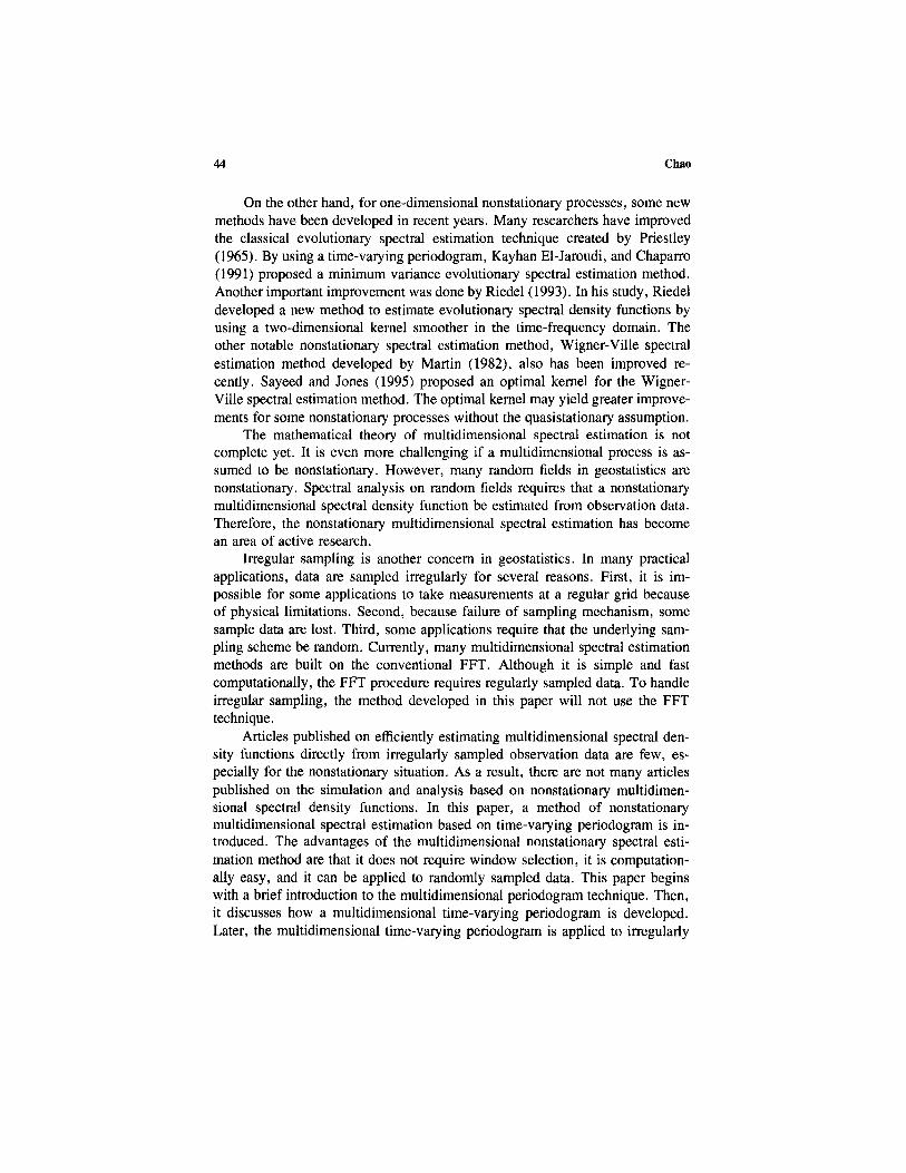
By substituting the irregularly sampled data into Equation (19), the esti-mated spectral density is calculated. f0 is selected so that -7r/2 < f01 < IT/2and - TT/2 < f02 < ir/2. A grid of 25 X 25 f0-values is used in the computationof Equation (19). To illustrate the nonstationarity, the estimated spectral densityfunction is evaluated at two spatial locations. Figure 2 shows the result at thelocation (s, t) = (5, 5).
In Figure 2, the estimated spectral density function is plotted on a 25 x25 grid. The horizontal axes represen f01 and f02. The vertical axis representsthe estimated spectral density. From Figure 2, one can see that the peak maybe correctly estimated.
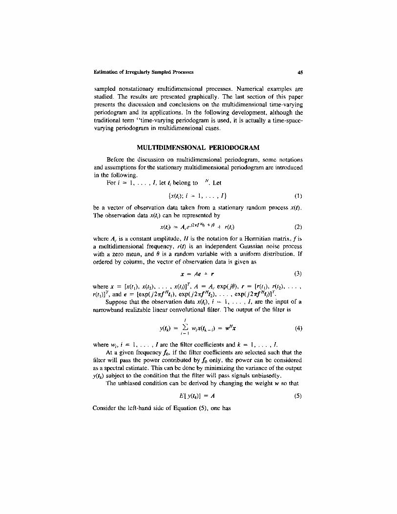
Figure 3 gives the estimated spectral density at the location (s, t) = (25,32). Notice that the scale on the vertical axis has been changed significantly,which indicates the effect of nonstationarity. The peak frequency in Figure 3also is correctly identified.
In the second example, the multidimensional time-varying periodogram isapplied to a nonstationary multidimensional storm model developed by Bras and
50 Chao
Figure 2. Estimated spectral density function at (t, s) = (5,5).
Rodriguez-Iturbe (1976). The rainfall intensity values of a storm are generatedby
where i(x, y, t) is the rainfall intensity at a point (x, y, t), R(x, y, t) is thestandard residual at (x, y, t) with a zero mean and unit variance, ia is the averageprecipitation at time (t - xi /u), aa is the standard deviation of precipitation attime (t - xi/u), and u is the average storm velocity in direction x.
The spatial correlation of rainfall intensities is assumed to be isotropic by
Figure 3. Estimated spectral density function at (t, s) =(25, 32).

Estimation of Irregularly Sampled Processes 51
Figure 4. Temporal average precipitation intensity of simulated storm.
Bras and Rodriguez-Iturbe (1976). The true peak frequency is expected to be atthe origin. With the average velocity u = 12 mi/hr and the temporal averageprecipitation and standard deviation given by Bras and Rodriguez-Iturbe (1976)(see Figs. 4 and 5), the point intensity is generated over a 20 x 20 square miledomain.
As pointed out by Bras and Rodriguez-Iturbe (1976), the point intensityhas little variation among different points in space at any given time duration,but the temporal behavior shows some significant variation. For a time durationof 14.33 hr, the largest variation occurs at the time interval (3.6 hr, 5.4 hr) andthe smallest variation occurs at the time interval (0 hr, 1.791 hr). 100 point-intensity values are selected randomly and the multidimensional time-varyingperiodogram procedure is applied to these data; then the estimated spectraldensity function is plotted in Figures 6 and 7. Again, to show the nonstationaryeifect, the estimated spectral density function is plotted for two different timeintervals. In Figure 6, the estimated spectral density function at (x, y, t) = (10,10, 4) is plotted. In Figure 7, the density function is plotted at (x, y, t) = (10,10, 1).
In Figure 6, the estimated spectral density is plotted for the time interval

52 Chao
Figure 5. Temporal standard deviation of simulated storm.
(3.6 hr, 5.4 hr) with the fixe f3 = 0. The time interval for Figure 7 is (0 hr,1.791 hr) on which the variation is about 20% of the variation on the intervalused in Figure 6. As in Figure 6, the estimated spectral density in Figure 7 isplotted on the f1 f2 domain with the fixef3 = 0.
Figure 6. Estimated spectral density function at (x, y, t)= (10, 10, 4).

Estimation of Irregularly Sampled Processes 53
Figure 7. Estimated spectral density function at (x, y, t) =(10, 10, 1).
CONCLUSIONS
There are many geostatistical variables which are considered as nonsta-tionary multidimensional random processes, such as the random processes gen-erated by earthquakes, storms, and wind-induced ocean wave elevation. Thespectral analysis of these random processes requires some reasonable approachto estimating spectral density functions from irregularly sampled data. In thispaper, a spectral estimation method based on multidimensional time-varyingperiodogram has been extended from the one-dimensional time-varying peri-odogram and has been applied to the data sampled irregularly from a multidi-mensional domain. Two numerical examples have been studied. From the es-timated spectral density functions, one can see that the peak frequencies havebeen identified correctly by the spectral estimation method developed in thispaper. For different points in a multidimensional domain, the nonstationaryeffect also can be seen by observing the changing peak values of the estimatedspectral density functions. These observations indicate that the multidimensionaltime-varying periodogram is a satisfactory spectral density estimation methodfor nonstationary multidimensional random processes. Because the method isbased on the assumption of nonstationarity, it has greater flexibility in con-ducting a spectral analysis.
Theoretically, the multidimensional time-varying method can be applied toany finite-dimensional spectral estimation problem. The advantages of themultidimensional nonstationary spectral estimation method are that it does notrequire window selection, it has better resolution power, and it can be appliedto randomly sampled data. To reduce the oscillation in an estimated spectraldensity function, a smoothing procedure should be considered to polish the finalresult.
54 Chao
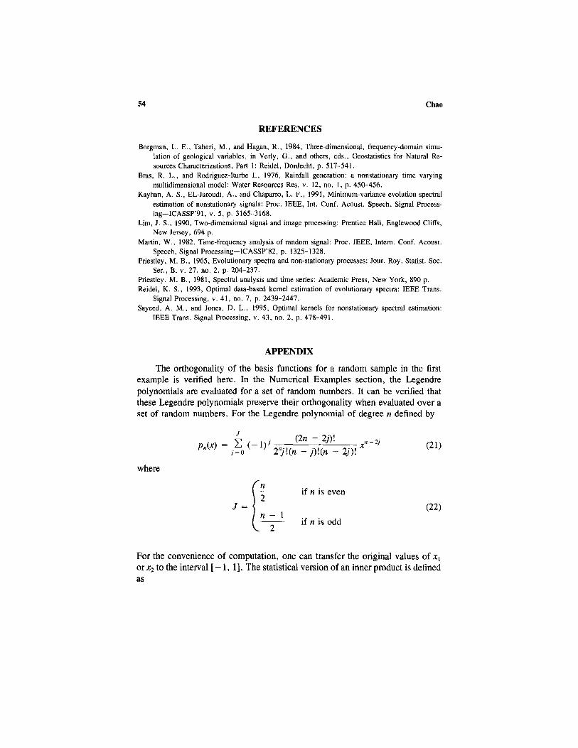
REFERENCES
Borgman, L. E., Taheri, M., and Hagan, R., 1984, Three-dimensional, frequency-domain simu-lation of geological variables, in Verly, G., and others, eds., Geostatistics for Natural Re-sources Characterizations, Part 1: Reidel, Dordecht, p. 517-541.
Bras, R. L., and Rodriguez-Iturbe I., 1976, Rainfall generation: a nonstationary time varyingmultidimensional model: Water Resources Res. v. 12, no. 1, p. 450-456.
Kayhan, A. S., EL-Jaroudi, A., and Chaparro, L. F., 1991, Minimum-variance evolution spectralestimation of nonstationary signals: Proc. IEEE, Int. Conf. Acoust. Speech, Signal Process-ing-ICASSP'91, v. 5, p. 3165-3168.
Lim, J. S., 1990, Two-dimensional signal and image processing: Prentice Hall, Englewood Cliffs,New Jersey, 694 p.
Martin, W., 1982, Time-frequency analysis of random signal: Proc. IEEE, Intern. Conf. Acoust.Speech, Signal Processing-ICASSP'82, p. 1325-1328.
Priestley, M. B., 1965, Evolutionary spectra and non-stationary processes: Jour. Roy. Statist. Soc.Ser., B, v. 27, no. 2, p. 204-237.
Priestley, M. B., 1981, Spectral analysis and time series: Academic Press, New York, 890 p.Reidel, K. S., 1993, Optimal data-based kernel estimation of evolutionary spectra: IEEE Trans.
Signal Processing, v. 41, no. 7, p. 2439-2447.Sayeed, A. M., and Jones, D. L., 1995, Optimal kernels for nonstationary spectral estimation:
IEEE Trans. Signal Processing, v. 43, no. 2, p. 478-491.
APPENDIX
The orthogonality of the basis functions for a random sample in the firstexample is verified here. In the Numerical Examples section, the Legendrepolynomials are evaluated for a set of random numbers. It can be verified thatthese Legendre polynomials preserve their orthogonality when evaluated over aset of random numbers. For the Legendre polynomial of degree n defined by
where
For the convenience of computation, one can transfer the original values of x1or x2 to the interval [ -1, 1]. The statistical version of an inner product is definedas
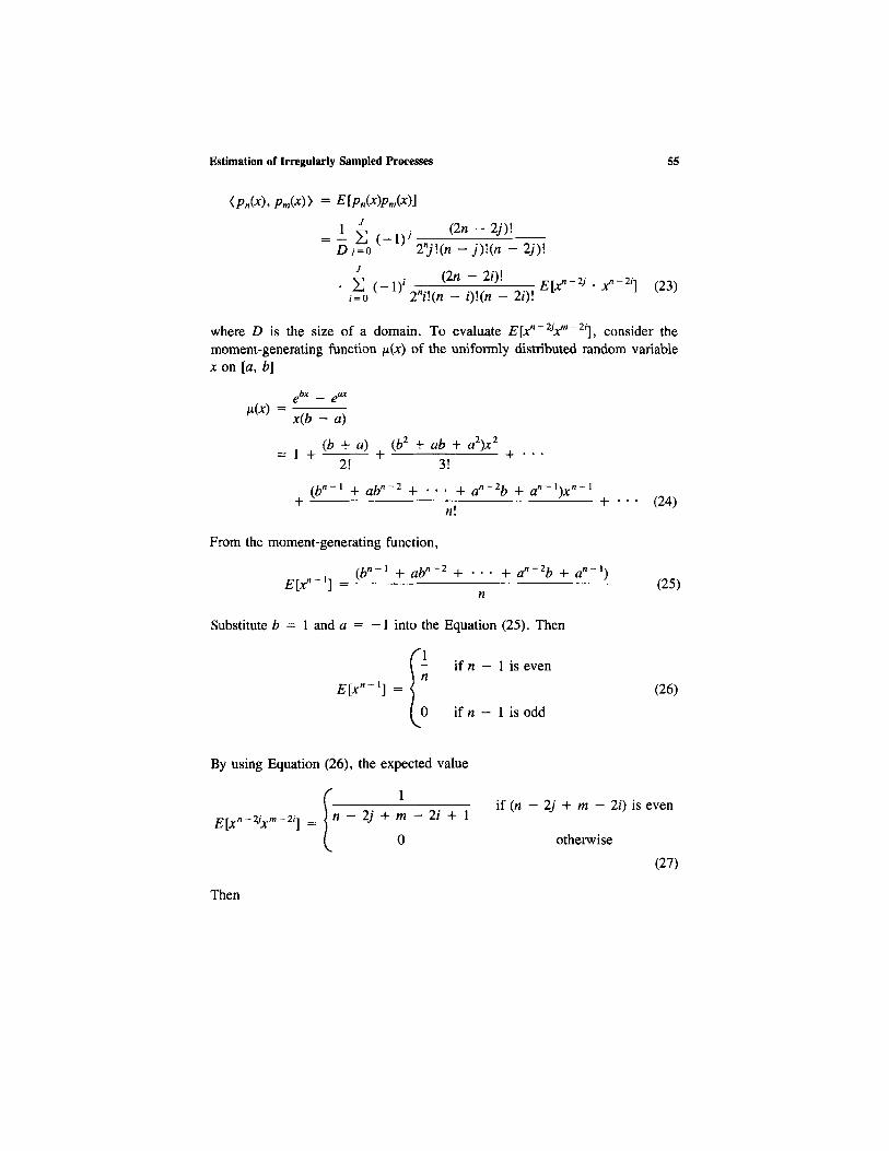
Estimation of Irregularly Sampled Processes 55
where D is the size of a domain. To evaluate E [ x n - 2 j x m - 2 i ] , consider themoment-generating function p(x) of the uniformly distributed random variablex on [a, b]
From the moment-generating function,
Substitute b - 1 and a = -1 into the Equation (25). Then
By using Equation (26), the expected value
Then
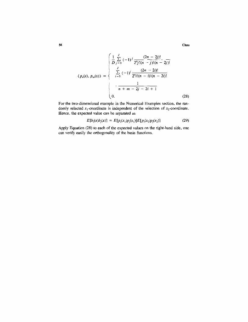
56 Chao
For the two-dimensional example in the Numerical Examples section, the ran-domly selected x1-coordinate is independent of the selection of x2-coordinate.Hence, the expected value can be separated as
Apply Equation (28) to each of the expected values on the right-hand side, onecan verify easily the orthogonality of the basis functions.