POLITEHNICA University Timisoara, Department of Hydrotechnics, 1A George Enescu, 300022, Timisoara, Romania, e-

mail: gheorghe.lazar@upt.ro

19

Buletinul Ştiinţific al Universităţii POLITEHNICA Timişoara

Seria HIDROTEHNICA

TRANSACTIONS on HYDROTECHNICS

Volume 59(73), Issue 2, 2014

Specific hydraulics related to a groundwater catchment

Gheorghe I. LAZĂR1 Marie-Alice GHITESCU2 Alina-Ioana POPESCU-BUSAN2

Albert Titus CONSTANTIN3 Şerban-Vlad NICOARĂ3

Abstract: The paper presents both, the study of a

ground water flow towards a series of catchment

drillings which are ran under different operational

schedule, and a flow simulation along the pipes network

and headrace supplying a small town of about 7200

inhabitants with fresh water under specific

requirements. The steady state ground water flow

numerical model considers a maximum captured

discharge of 20.00 l/s, obtained from 6 running drillings

out of 9 corresponding to several specific operation

situations. A daily water demand distribution is assumed

(the hourly variation ratios for the increased

consumption interval considered from 0.51 to 1.37),

which leads to a maximum water flow reached in the

network of 1.64 m3/min. The hourly water volume

required for the supply system is stored up by a

reservoir placed about 12km from the catchment line.

Several relative pumps rotation speed values are

considered in such a way that the working parameters of

the running system to be optimized.

Keywords: groundwater flow, underground water

catchment, pipes network.

1. INTRODUCTION

The Salsig Groundwater Catchment is situated on S-

W of the homonym village on the left bank of Somes

River, specifically in the alluvial fan formed by the

tributary Salaj Creek. The hydrotechnical study is

based on general data regarding the geo-morphology

and hydro-geology of the area corresponding to the

nine catchment drillings in the Somes River flood

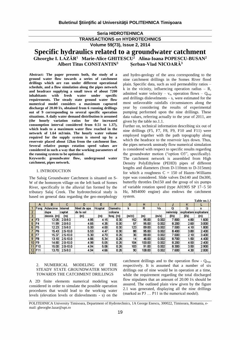
plain. Specific data, such as soil permeability ratios –

k in the vicinity, influencing operation radius – R,

admitted water velocity – va, operation flows – Qexp

and drillings dislevelments – s, were estimated for the

most unfavorable rainfalls circumstances along the

year by considering the results of experimental

pumping performed upon the nine drillings. These

data values, referring actually to the year of 2011, are

given by the table no.1.1.

Further on, technical information describing six out of

nine drillings (F5, F7, F8, F9, F10 and F11) were

employed together with the path topography along

which the headrace to the reservoir lays down. Thus,

the pipes network unsteady flow numerical simulation

is considered with respect to specific results regarding

the groundwater motion (“option O3”, specifically).

The catchment network is assembled from High

Density PolyEthylene (PEHD) pipes of different

lengths and diameters (from D-110mm to D-315mm)

for which a roughness C = 150 of HazenWilliams

type was considered. Slide valves Dn140 and Dn300,

butterfly throttles Dn150 and the group of six pumps

of variable rotation speed (type A01905 SP 175 50

Hz, MS4000 engine) also endows the catchment

system. Table no.1.1

2. NUMERICAL MODELING OF THE

STEADY STATE GROUNDWATER MOTION

TOWARDS THE CATCHMENT DRILLINGS

A 2D finite elements numerical modeling was

considered in order to simulate the possible operation

procedures that would lead to the working water

levels (elevation levels or dislevelments - s) on the

catchment drillings and to the operation flow - Qexp,

respectively. It is assumed that a number of six

drillings out of nine would be in operation at a time,

while the requirement regarding the total discharged

flow stipulates that an amount of 20.00 l/s should be

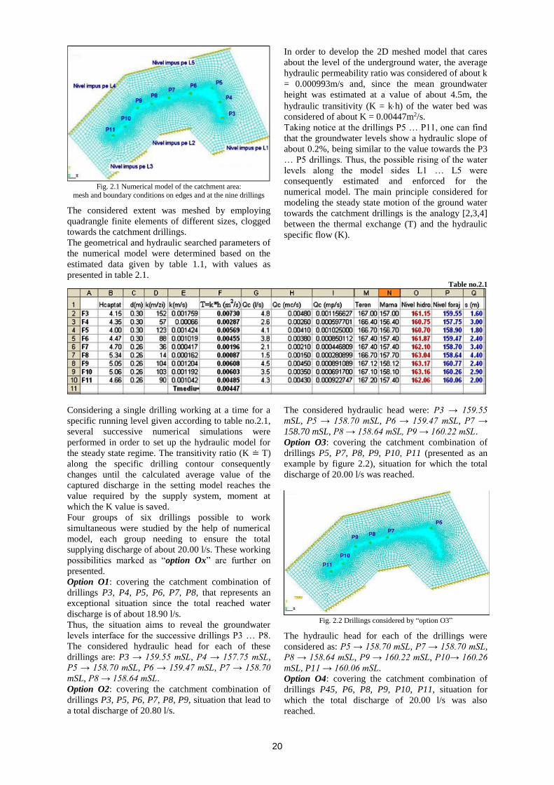
assured. The outlined plain view given by the figure

2.1 was generated, displaying all the nine drillings

(marked as P3 … P11 in the numerical model).

20

Fig. 2.1 Numerical model of the catchment area:

mesh and boundary conditions on edges and at the nine drillings

The considered extent was meshed by employing

quadrangle finite elements of different sizes, clogged

towards the catchment drillings.

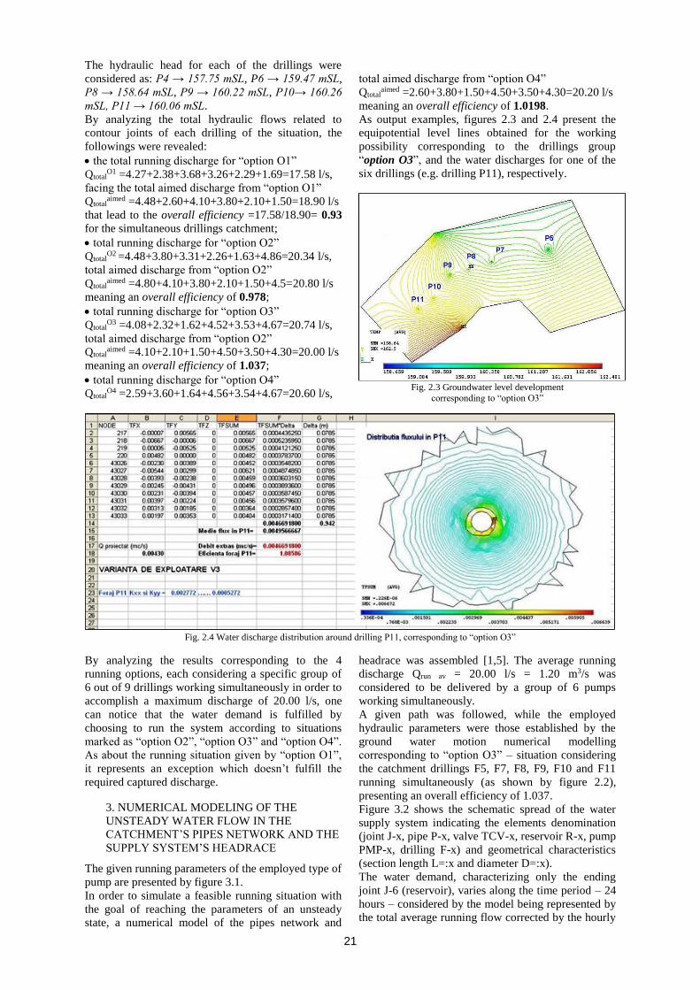
The geometrical and hydraulic searched parameters of

the numerical model were determined based on the

estimated data given by table 1.1, with values as

presented in table 2.1.

In order to develop the 2D meshed model that cares

about the level of the underground water, the average

hydraulic permeability ratio was considered of about k

= 0.000993m/s and, since the mean groundwater

height was estimated at a value of about 4.5m, the

hydraulic transitivity (K = kh) of the water bed was

considered of about K = 0.00447m2/s.

Taking notice at the drillings P5 … P11, one can find

that the groundwater levels show a hydraulic slope of

about 0.2%, being similar to the value towards the P3

… P5 drillings. Thus, the possible rising of the water

levels along the model sides L1 … L5 were

consequently estimated and enforced for the

numerical model. The main principle considered for

modeling the steady state motion of the ground water

towards the catchment drillings is the analogy [2,3,4]

between the thermal exchange (T) and the hydraulic

specific flow (K).

Table no.2.1

Considering a single drilling working at a time for a

specific running level given according to table no.2.1,

several successive numerical simulations were

performed in order to set up the hydraulic model for

the steady state regime. The transitivity ratio (K ≐ T)

along the specific drilling contour consequently

changes until the calculated average value of the

captured discharge in the setting model reaches the

value required by the supply system, moment at

which the K value is saved.

Four groups of six drillings possible to work

simultaneous were studied by the help of numerical

model, each group needing to ensure the total

supplying discharge of about 20.00 l/s. These working

possibilities marked as “option Ox” are further on

presented.

Option O1: covering the catchment combination of

drillings P3, P4, P5, P6, P7, P8, that represents an

exceptional situation since the total reached water

discharge is of about 18.90 l/s.

Thus, the situation aims to reveal the groundwater

levels interface for the successive drillings P3 … P8.

The considered hydraulic head for each of these

drillings are: P3 → 159.55 mSL, P4 → 157.75 mSL,

P5 → 158.70 mSL, P6 → 159.47 mSL, P7 → 158.70

mSL, P8 → 158.64 mSL.

Option O2: covering the catchment combination of

drillings P3, P5, P6, P7, P8, P9, situation that lead to

a total discharge of 20.80 l/s.

The considered hydraulic head were: P3 → 159.55

mSL, P5 → 158.70 mSL, P6 → 159.47 mSL, P7 →

158.70 mSL, P8 → 158.64 mSL, P9 → 160.22 mSL.

Option O3: covering the catchment combination of

drillings P5, P7, P8, P9, P10, P11 (presented as an

example by figure 2.2), situation for which the total

discharge of 20.00 l/s was reached.

Fig. 2.2 Drillings considered by “option O3”

The hydraulic head for each of the drillings were

considered as: P5 → 158.70 mSL, P7 → 158.70 mSL,

P8 → 158.64 mSL, P9 → 160.22 mSL, P10→ 160.26

mSL, P11 → 160.06 mSL.

Option O4: covering the catchment combination of

drillings P45, P6, P8, P9, P10, P11, situation for

which the total discharge of 20.00 l/s was also

reached.

21

The hydraulic head for each of the drillings were

considered as: P4 → 157.75 mSL, P6 → 159.47 mSL,

P8 → 158.64 mSL, P9 → 160.22 mSL, P10→ 160.26

mSL, P11 → 160.06 mSL.

By analyzing the total hydraulic flows related to

contour joints of each drilling of the situation, the

followings were revealed:

• the total running discharge for “option O1”

QtotalO1 =4.27+2.38+3.68+3.26+2.29+1.69=17.58 l/s,

facing the total aimed discharge from “option O1”

Qtotalaimed =4.48+2.60+4.10+3.80+2.10+1.50=18.90 l/s

that lead to the overall efficiency =17.58/18.90= 0.93

for the simultaneous drillings catchment;

• total running discharge for “option O2”

QtotalO2 =4.48+3.80+3.31+2.26+1.63+4.86=20.34 l/s,

total aimed discharge from “option O2”

Qtotalaimed =4.80+4.10+3.80+2.10+1.50+4.5=20.80 l/s

meaning an overall efficiency of 0.978;

• total running discharge for “option O3”

QtotalO3 =4.08+2.32+1.62+4.52+3.53+4.67=20.74 l/s,

total aimed discharge from “option O2”

Qtotalaimed =4.10+2.10+1.50+4.50+3.50+4.30=20.00 l/s

meaning an overall efficiency of 1.037;

• total running discharge for “option O4”

QtotalO4 =2.59+3.60+1.64+4.56+3.54+4.67=20.60 l/s,

total aimed discharge from “option O4”

Qtotalaimed =2.60+3.80+1.50+4.50+3.50+4.30=20.20 l/s

meaning an overall efficiency of 1.0198.

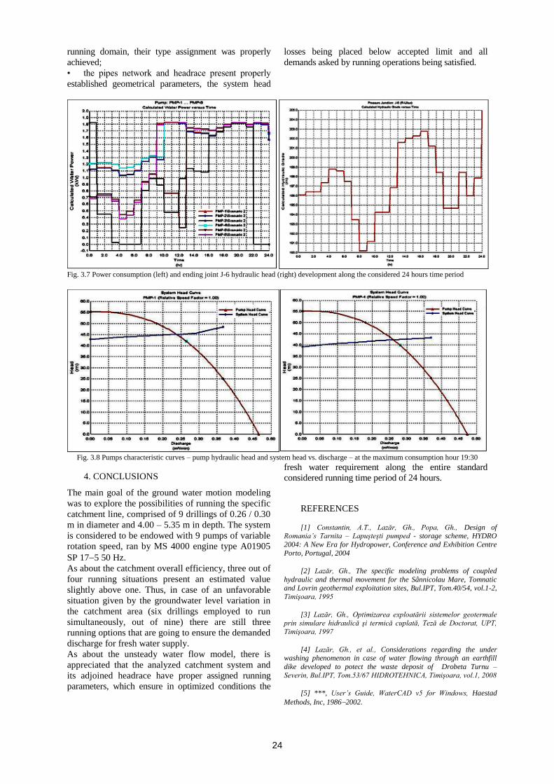
As output examples, figures 2.3 and 2.4 present the

equipotential level lines obtained for the working

possibility corresponding to the drillings group

“option O3”, and the water discharges for one of the

six drillings (e.g. drilling P11), respectively.

Fig. 2.3 Groundwater level development

corresponding to “option O3”

Fig. 2.4 Water discharge distribution around drilling P11, corresponding to “option O3”

By analyzing the results corresponding to the 4

running options, each considering a specific group of

6 out of 9 drillings working simultaneously in order to

accomplish a maximum discharge of 20.00 l/s, one

can notice that the water demand is fulfilled by

choosing to run the system according to situations

marked as “option O2”, “option O3” and “option O4”.

As about the running situation given by “option O1”,

it represents an exception which doesn’t fulfill the

required captured discharge.

3. NUMERICAL MODELING OF THE

UNSTEADY WATER FLOW IN THE

CATCHMENT’S PIPES NETWORK AND THE

SUPPLY SYSTEM’S HEADRACE

The given running parameters of the employed type of

pump are presented by figure 3.1.

In order to simulate a feasible running situation with

the goal of reaching the parameters of an unsteady

state, a numerical model of the pipes network and

headrace was assembled [1,5]. The average running

discharge Qrun av = 20.00 l/s = 1.20 m3/s was

considered to be delivered by a group of 6 pumps

working simultaneously.

A given path was followed, while the employed

hydraulic parameters were those established by the

ground water motion numerical modelling

corresponding to “option O3” – situation considering

the catchment drillings F5, F7, F8, F9, F10 and F11

running simultaneously (as shown by figure 2.2),

presenting an overall efficiency of 1.037.

Figure 3.2 shows the schematic spread of the water

supply system indicating the elements denomination

(joint J-x, pipe P-x, valve TCV-x, reservoir R-x, pump

PMP-x, drilling F-x) and geometrical characteristics

(section length L=:x and diameter D=:x).

The water demand, characterizing only the ending

joint J-6 (reservoir), varies along the time period – 24

hours – considered by the model being represented by

the total average running flow corrected by the hourly

22

variation ratio 0.51 ÷ 1.37 along one day given by

figure 3.3. Consequently, figure 3.4 gives the water

demand behavior along the time period, while the

limit values for required flow are Qrun_min = 0.61

m3/min and Qrun_max = 1.64 m3/min, respectively.

Fig. 3.1 MS4000 pumps characteristics

The boundary conditions considered on a data base in

order to solve the equations system generated by the

numerical model regard the minimum water levels in

catchment drillings area (PMP-1 → Ha=158.7m, PMP-

2 → Ha=158.7m, PMP-3 → Ha=158.64m, PMP-4 →

Ha=160.22m, PMP-5 → Ha=160.26m and PMP-6 →

Ha=160.06m) and in the same time the running

conditions assigned to the pumps by the relative

rotation ratio for an optimal work (minimum power

consumption).

All running parameters corresponding to the

considered group of six simultaneous working pumps

were obtained through the numerical simulation. As

an output example, figure 3.5 presents the water flows

through the components of the system formed by the

headrace and the pipes network for one specific

situation, i.e. the one developed at the maximum

consumption moment of 19:30.

The minimum water demand, happening at 04:00, is

0.61 m3/min, the pumped discharge at PMP-5 and PMP-

6 being 0.06 m3/min, while PMP-3 is turned off. As

regarding the maximum water demand at 19:30, the

water flow at the reservoir entrance is 1.64 m3/min,

while at the 6 pumps, all working, the water discharges

are as follows: PMP-1 → Q = 0.27 m3/min, PMP-2 →

Q = 0.27 m3/min, PMP-3 → Q = 0.27 m3/min, PMP-4

→ Q = 0.28 m3/min; PMP-5 → Q = 0.28 m3/min, PMP-

6 → Q = 0.28 m3/min.

The pumped water discharge aside of hydraulic head

behavior in time for the simultaneous working group of

6 pumps along a 24 hours time period is given by figure

3.6. Further on, figure 3.7 presents power consumption

development for the considered time period and the

hydraulic head produced at ending joint J-6 (reservoir

entrance), respectively.

Fig. 3.2 Water catchment system: pipes network and headrace [5]

As regarding the time development of the hydraulic

head, one can notice that at the minimum consumption

moments the pumps head upper limit reaches about

41.00m and then dropping towards the lower limit of

about 33.00m, while at the maximum consumption

moments the head goes for the upper limit of about

48.00m and drops at about 40.00m.

As a representative situation, figure 3.8 brings the

characteristic curves – the pump hydraulic head and the

system head vs. discharge – of two pumps (PMP-1 and

PMP-4) working simultaneously at the maximum

consumption hour 19:30.

23

Fig. 3.3 Water demand hourly variation ratio along one day Fig. 3.4 Water demand behavior along one day at joint J-6

Fig. 3.5 Water flow development at two specific moments: top h04:00, below h19:30

Fig. 3.6 Pumps water discharge (left) and hydraulic head (right) behavior for the 24 hours time period

By studying the results and the processed graphic

outputs, the followings can be found:

• the head loss along the longest path of the scheme at

the moment of maximum consumption is 5.94m (the

drop from 200.56 to 194.62 in figure 3.9);

• the hydraulic head of the system ending point -

reservoir entrance section - at the most demanding

moment, 19:30 hours, when the maximum supplied

discharge is of 1.64 m3/min, reaches the minimum level

of 194.62m, a value still above the maximum water

level in this storing basin (192.00m) with 2.62m;

• at the moment of maximum consumption each pump

runs near the point of optimum work (BEP);

• the power consumed by each pump along the running

period of 24 hours leads towards an optimum cumulated

value;

• since the pumps endowing the catchment drillings

(P5, P7, P8, P9, P10, P11) work in their optimum

24

running domain, their type assignment was properly

achieved;

• the pipes network and headrace present properly

established geometrical parameters, the system head

losses being placed below accepted limit and all

demands asked by running operations being satisfied.

Fig. 3.7 Power consumption (left) and ending joint J-6 hydraulic head (right) development along the considered 24 hours time period

Fig. 3.8 Pumps characteristic curves – pump hydraulic head and system head vs. discharge – at the maximum consumption hour 19:30

4. CONCLUSIONS

The main goal of the ground water motion modeling

was to explore the possibilities of running the specific

catchment line, comprised of 9 drillings of 0.26 / 0.30

m in diameter and 4.00 – 5.35 m in depth. The system

is considered to be endowed with 9 pumps of variable

rotation speed, ran by MS 4000 engine type A01905

SP 175 50 Hz.

As about the catchment overall efficiency, three out of

four running situations present an estimated value

slightly above one. Thus, in case of an unfavorable

situation given by the groundwater level variation in

the catchment area (six drillings employed to run

simultaneously, out of nine) there are still three

running options that are going to ensure the demanded

discharge for fresh water supply.

As about the unsteady water flow model, there is

appreciated that the analyzed catchment system and

its adjoined headrace have proper assigned running

parameters, which ensure in optimized conditions the

fresh water requirement along the entire standard

considered running time period of 24 hours.

REFERENCES

[1] Constantin, A.T., Lazăr, Gh., Popa, Gh., Design of Romania’s Tarnita – Lapuşteşti pumped - storage scheme, HYDRO

2004: A New Era for Hydropower, Conference and Exhibition Centre

Porto, Portugal, 2004

[2] Lazăr, Gh., The specific modeling problems of coupled

hydraulic and thermal movement for the Sânnicolau Mare, Tomnatic and Lovrin geothermal exploitation sites, Bul.IPT, Tom.40/54, vol.1-2,

Timişoara, 1995

[3] Lazăr, Gh., Optimizarea exploatării sistemelor geotermale prin simulare hidraulică şi termică cuplată, Teză de Doctorat, UPT,

Timişoara, 1997

[4] Lazăr, Gh., et al., Considerations regarding the under washing phenomenon in case of water flowing through an earthfill

dike developed to potect the waste deposit of Drobeta Turnu –

Severin, Bul.IPT, Tom.53/67 HIDROTEHNICA, Timişoara, vol.1, 2008

[5] ***, User’s Guide, WaterCAD v5 for Windows, Haestad

Methods, Inc, 19862002.