special issue on leonhard paul euler’s: mixed type partial...

Special Issue on Leonhard Paul Euler’s:

Mixed Type Partial Differential Equations (MT. PDE)

Volume 8 Number M07 March 2007

ISSN 0973-1377 (Print) ISSN 0973-7545 (Online)

International Journal of AppliedMathematics & Statistics

ISSN 0973-1377

Editorial Board

Executive Editor:

Tanuja Srivastava Department of Mathematics,

Indian Institute of Technology Roorkee-247667,INDIA

Email: [email protected]

Editors-in-Chief:

Florentin Smarandache Department of Mathematics & Sciences, University of New Mexico, USA. E-mail: [email protected]

R. K. S. Rathore

Department of Mathematics, Indian Institute of Technology, Kanpur, INDIA E-mail: [email protected]

Editors

Delfim F. M. Torres University of Aveiro Portugal Alexandru Murgu British Tel. Net. Research Centre UK Edward Neuman Southern Illinois University USA Hans Gottlieb Griffith University Australia Akca Haydar United Arab Emiartes University UAE Somesh Kumar Indian Institute of Technology, Kharagpur India

Associate Editors:

Alexander Grigorash University of Ulster U.K.

Bogdan G. Nita Montclair State University USA

Sukanto Bhattacharya Alaska Pacific University USA

Rogemar S Mamon University of Western Ontario Canada

Ferhan Atici Western Kentucky University USA

Karen Yagdjian University of Texas-Pan American USA

Rui Xu University of West Georgia USA

Alexander A. Katz St. John's University USA

Associate Editors: Contd….

Eduardo V. Teixeira Rutgers University USA

Weijiu Liu University of Central Arkansas USA

Wieslaw A. Dudek Wroclaw University of Technology Poland

Ki-Bong Nam University of Wisconsin, Whitewater USA

Diego Ernesto Dominici State University of New York at New Paltz USA

Ming Fang Norfolk State University USA

Hemant Pendharkar Worcester State College USA

Wen-Xiu Ma University of South Florida USA

V. Ravichandran University Sains Malaysia Malaysia

Piotr Matus Institute of Mathematics of NASB Belarus

Mustafa Bayram Yildiz Teknik Üniversitesi Turkey

Rodrigo Capobianco Guido University of S.ao Paulo Brazil

Song Wang University of Western Australia Australia

Tianzi Jiang Institute of Automation, CAS PR China

Henryk Fuks Brock University Canada

Nihal Yilmaz Ozgur Balikesir University Turkey

Muharem Avdispahic University of Sarajevo Bosnia

Xiao-Xiong Gan Morgan State University USA

Assistant Editors:

Irene Sciriha University of Malta Malta Doreen De Leon California State University USA Anahit Ann Galstyan University of Texas-Pan American USA Oliver Jones California State University USA Jose Almer T. Sanqui Appalachian State University USA Miranda I. Teboh-Ewungkem Lafayette College USA Guo Wei University of North Carolina at Pembroke USA Michael D. Wills Weber State University USA Alain S. Togbe Purdue University North Central USA Samir H. Saker Mansoura University Egypt Ganatsiou V. Chrysoula University of Thessaly Greece Bixiang Wang New Mexico Institute of Mining & Technology USA Andrei Volodin University of Regina Canada Mohammad Sal Moslehian Ferdowsi University Iran Ashwin Vaidya University of North Carolina - Chapel Hill USA Anna Karczewska University of Zielona Góra Poland Xiaoli Li University of Birmingham UK Guangyi Chen Canadian Space Agency Canada Clemente Cesarano University of Roma Italy Rãzvan Rãducanu Al. I. Cuza University Romania Fernando M. Lucas Carapau University of Évora Portugal Alireza Abdollahi University of Isfahan Iran Ay e Altın Hacettepe University Turkey

Special Issue on Leonhard Paul Euler’s:

Functional Equations and Inequalities (F. E. I.)

Special Editor-in-Chief

John Michael Rassias

Professor of Mathematics, National and Capodistrian, University of Athens, Greece

Guest Editors

Jewgeni H. Dshalalow Florida Institute of Technology, Division of Mathematical Sciences,

College of Science, Melbourne, FL 32901, U. S. A.

Valerii A. Faiziev Tver State Agricultural Academy, Tver Sakharovo, RUSSIA

David Goss The Ohio State University, Department of Mathematics

231 W. 18th Ave., Columbus, Ohio 43210, U. S. A.

Johnny Henderson Baylor University, Department of Mathematics

Waco, Texas 76798-7328, U. S. A.

T. Kusano Fukuoka University, Department of Applied Mathematics,

Faculty of Science, Fukuoka, 814-0180, JAPAN

Alexander G. Kuz’min St Petersburg State University

Institute of Mathematics and Mechanics 28 University Ave., 198504 St Petersburg, RUSSIA

Xuerong Mao University of Strathclyde

Department of Statistics and Modelling Science, Glasgow G1 1XH, U. K.

Shuji Watanabe Gunma University

Department of Mathematics, Faculty of Engineering 4-2 Aramaki-machi, Maebashi 371-8510, JAPAN

Guochun Wen Peking University

School of Mathematical Sciences, Beijing 100871, CHINA

International Journal of Applied Mathematics & Statistics

Contents

Volume 8 Number M07 March 2007

Preface 6

Initial-oblique derivative problem for nonlinear parabolic equations in high dimensional domains

D. Chen and G. Wen

8

Some solutions of generalized Rassias’s equation

A. Hasanov

20

The solution of the Cauchy problem for generalized Euler-Poisson-Darboux equation

A. Hasanov

30

Uniqueness of the solution of one non-local boundary value problem for the mixed parabolic type equation

E. T. Karimov

44

Non-uniqueness of transonic flow past a flattened airfoil

A. G. Kuz’min

49

Multiplier methods for mixed type equations

K. R. Payne

58

Tricomi-Protter problem of nD mixed type equations

J. M. Rassias

76

Fundamental solutions of two degenerated elliptic equations and solutions of boundary value problems in infinite area

J. M. Rassias and A. Hasanov

87

Solvability of the oblique derivative problem for second order equations of mixed type with nonsmooth degenerate curve

J. M. Rassias and G. Wen

96

PREFACE

This Euler’s commemorating volume entitled : Functional Equations , Integral Equations, Differential Equations and Applications (F. I. D. A),is a forum for exchanging ideas among eminent mathematicians and physicists, from many parts of the world, as a tribute to the tri-centennial birthday anniversary of Leonhard Paul Euler (April 15,1707 A.D., b. in Basel – September 18, 1783 A.D., d. in St. Petersburg). This 998 pages long collection is composed of outstanding contributions in mathematical and physical equations and inequalities and other fields of mathematical, physical and life sciences. In addition, this anniversary volume is unique in its target, as it strives to represent a broad and highly selected participation from across and beyond the scientific and technological country regions. It is intended to boost the cooperation among mathematicians and physicists working on a broad variety of pure and applied mathematical areas. Moreover, this new volume will provide readers and especially researchers with a detailed overview of many significant insights through advanced developments on Euler’s mathematics and physics. This transatlantic collection of mathematical ideas and methods comprises a wide area of applications in which equations, inequalities and computational techniques pertinent to their solutions play a core role.Euler’s influence has been tremendous on our everyday life, because new tools have been developed, and revolutionary research results have been achieved , bringing scientists of exact sciences even closer, by fostering the emergence of new approaches, techniques and perspectives. The central scope of this commemorating 300birthday anniversary volume is broad, by deeper looking at the impact and the ultimate role of mathematical and physical challenges, both inside and outside research institutes, scientific foundations and organizations. We have recently observed a more rapid development in the areas of research of Euler worldwide. Leonhard P. Euler (1707-1783) was actually the most influential mathematician and prolific writer of the eighteenth century, by having contributed to almost all the fundamental fields of mathematics and mathematical physics. In calculus of variations, according to C. Caratheodory, Euler’s work: Methodus inveniendi lineas curves…(1740 A.D.) was one of the most beautiful works ever written. Euler was dubbed Analysis Incarnate by his peers for his incredible ability. He was especially great from his writings and that produced more academic work on mathematics than anyone. He could produce an entire new mathematical paper in about thirty minutes and had huge piles of his works lying on his desk. It was not uncommon to find Analysis Incarnate ruminating over a new subject with a child on his lap. This volume is suitable for graduate students and researchers interested in functional equations, integral equations and differential equations and would make an ideal supplementary reading or independent study research text. This item will also be of interest to those working in other areas of mathematics and physics. It is a work of great interest and enjoyable read as well as unique in market.

This Euler’s volume (F. I. D. A.) consists of six (6) issues containing various parts of contemporary pure and applied mathematics with emphasis to Euler’s mathematics and physics. It contains sixty eight (68) fundamental research papers of one hundred one (101) outstanding research contributors from twenty seven (27) different countries. In particular, these contributors come from: Algerie (1 contributor); Belgique (2); Bosnia and Herzegovina (2); Brazil (2); Bulgaria (3); China (9); Egypt (1); France (3); Greece (2); India (8); Iran (3); Italy (1); Japan (7); Korea (7); Morocco (3); Oman (2); Poland (3); R. O. Belarus (8); Romania (2); Russia (3); Saudi Arabia (1); Serbia and Montenegro (5); The Netherlands (3); U. A. Emirates (1);U. K. (2); U. S. A. (15); Uzbekistan (2).

First Issue (F. E. I.) consisting of 14 research papers, 181 pages long, contains various parts of Functional Equations and Inequalities,namely:Euler’s Life and Work, Ulam stability, Hyers – Ulam stability and Ulam – Gavruta - Rassias stability of functional equations, Euler – Lagrange type and Euler – Lagrange – Rassias quadratic mappings in Banach and Hilbert spaces, Aleksandrov and isometry Ulam stability problems, stability of Pexider and Drygas functional equations, alternative of fixed point, and Hyers - Ulam stability of differential equations.

International Journal of Applied Mathematics & Statistics,ISSN 0973-1377 (Print), ISSN 0973-7545 (Online)Copyright © 2007 by IJAMAS, CESER; March 2007, Vol. 8, No. M07, 6-7

Second Issue (MT. PDE) consisting of 9 research papers, 117 pages long, contains various parts of Mixed Type Partial Differential Equations,namely:Tricomi - Protter problem of nD mixed type partial differential equations, solutions of generalized Rassias’ equation, degenerated elliptic equations, mixed type oblique derivative problem, Cauchy problem for Euler – Poisson - Darboux equation, non - local boundary value problems, non-uniqueness of transonic flow past a flattened airfoil, multiplier methods for mixed type equations. Third Issue (F . D . E.) consisting of 9 research papers, 146 pages long, contains various parts of Functional and Differential Equations,namely:Iterative method for singular Sturm - Liouville problems, Euler type boundary value problems in quantum mechanics, positive solutions of boundary value problems, controllability of impulsive functional semi-linear differential inclusions in Frechet spaces, asymptotic properties of solutions of the Emden-Fowler equation, comparison theorems for perturbed half-linear Euler differential equations, almost sure asymptotic estimations for solutions of stochastic differential delay equations, difference equations inspired by Euler’s discretization method, extended oligopoly models. Fourth Issue (D. E. I.) consisting of 9 research papers, 160 pages long, contains various parts of Differential Equations and Inequalities,namely:New spaces with wavelets and multi-fractal analysis, mathematical modeling of flow control and wind forces, free convection in conducting fluids, distributions in spaces, strong stability of operator– differential equations, slope – bounding procedure, sinc methods and PDE, Fourier type analysis and quantum mechanics. Fifth Issue (DS. IDE.) consisting of 9 research papers, 159 pages long, contains various parts of Dynamical Systems and Integro - Differential Equations,namely:Semi-global analysis of dynamical systems, nonlinear functional-differential and integral equations, optimal control of dynamical systems, analytical and numerical solutions of singular integral equations, chaos control of classes of complex dynamical systems, second order integro-differential equation, integro-differential equations with variational derivatives generated by random partial integral equations, inequalities for positive operators, strong convergence for a family of non-expansive mappings. Sixth Issue (M. T. A.) consisting of 18 research papers, 231 pages long, contains various parts of Mathematical Topics and Applications,namely:Maximal subgroups and theta pairs in a group, Euler constants on algebraic number fields, characterization of modulated Cox measures on topological spaces, hyper-surfaces with flat r-mean curvature and Ribaucour transformations, Leonhard Euler’s methods and ideas live on in the thermodynamic hierarchical theory of biological evolution, zeroes of L-series in characteristic p, Beck’s graphs, best co-positive approximation function, Convexity in the theory of the Gamma function, analytical and differential – algebraic properties of Gamma function, Ramanujan’s summation formula and related identities, ill – posed problems, zeros of the q-analogues of Euler polynomials, Eulerian and other integral representations for some families of hyper-geometric polynomials, group C*-algebras and their stable rank, complementaries of Greek means to Gini means, class of three- parameter weighted means, research for Bernoulli’s inequality.

Deep gratitude is due to all those Guest Editors and Contributors who helped me to carry out this intricate project. My warm thanks to my family: Matina- Mathematics Ph. D. candidate of the Strathclyde University (Glasgow, United Kingdom), Katia- Senior student of Archaeology and History of Art of the National and Capodistrian University of Athens (Greece), and Vassiliki- M. B. A. of the University of La Verne, Marketing Manager in a FMCG company (Greece). Finally I express my special appreciation to: The Executive Editor of the International Journal of Applied Mathematics & Statistics (IJAMAS)Dr. Tanuja Srivastava for her nice cooperation and great patience.


Special Editor-in-Chief of Euler’s volume F. I. D. A. – IJAMAS.National and Capodistrian University of Athens, Greece E-mail: [email protected]; [email protected] URL: http://www.primedu.uoa.gr/~jrassias/

Int. J. Appl. Math. Stat.; Vol. 8, No. M07, March 2007 7

Initial-Oblique Derivative Problem for Nonlinear ParabolicEquations in High Dimensional Domains

Dechang Chen1 and Guochun Wen2

1Department of Preventive Medicine and BiometricsUniformed Services University of the Health Sciences

MD 20814, USAE-mail: [email protected]

2School of Mathematical SciencesPeking University

Beijing 100871, ChinaE-mail: [email protected]

ABSTRACT

In this paper, we discuss some initial-boundary value problems for nonlinear nondiver-

gent parabolic equations of second order in high dimensional domains, where coefficients

of equations are measurable in multiply connected domains. We focus on initial-oblique

derivative problems. The estimates of solutions for the initial-boundary value problems are

given, and then the solvability result is derived. The results in this paper are the develop-

ment of the corresponding work in [1, 3, 4].

Keywords: initial-oblique derivative problems, nonlinear parabolic equations, high dimen-

sional domains.

2000 Mathematics Subject Classification: 35K15, 35K20, 35K60.

1 Formulation of Initial-Boundary Value Problems for Nonlinear Parabolic Equa-tions

Let Ω be a bounded multiply connected domain in RN with the boundary ∂Ω ∈ C 2α (0 < α < 1).

Set Q = Ω × I, where I is the interval 0 < t ≤ T , 0 < T < ∞. Let ∂Q = ∂Q1 ∪ ∂Q2 or

S = S1 ∪ S2 denote the parabolic boundary, where ∂Q1 = S1 = Ω × t = 0 is the bottom and

∂Q2 = S2 = ∂Ω × I is the lateral boundary. We consider the nonlinear parabolic equation of

second order

F (x, t, u,Dxu,D2xu) − Hut = 0 in Q,

where H is a positive number, and Dxu = (uxi), D2xu = (uxixj ). Under certain conditions, the

above equation can be written as

N∑i,j=1

aijuxixj +N∑

i=1

biuxi + cu − Hut = f in Q, (1.1)


where

aij =∫ 1

0Fτrij (x, t, u, p, τr)dτ, bi =

∫ 1

0Fτpi(x, t, u, τp, 0)dτ,

c=∫ 1

0Fτu(x, t, τu, 0, 0)dτ, f = −F (x, t, 0, 0, 0),

with r = D2xu = (rij) =

( ∂2u

∂xi∂xj

), p = Dxu = (pi) =

( ∂u

∂xi

).

Suppose that (1.1) satisfies Condition C, i.e. for arbitrary functions u1(x, t), u2(x, t) ∈ C1,0β,β/2(Q)∩

W 2,12 (Q) (0 < β < 1), F (x, t, u,Dxu, D2

xu) satisfies the condition

F (x, t, u1, Dxu1, D2xu1) − F (x, t, u2, Dxu2, D

2xu2)

=N∑

i,j=1

aijuxixj +N∑

i=1

biuxi + cu,

where u = u1 − u2, W 2,12 (Q) = W 2,0

2 (Q) ∩ W 0,12 (Q), and

aij =∫ 1

0Fuxixj

(x, t, u, p, r)dτ, bi =∫ 1

0Fuxi

(x, t, u, p, r)dτ,

c =∫ 1

0Fu(x, t, u, p, r)dτ, u = u2 + τ(u1 − u2),

p = Dx[u2 + τ(u1 − u2)], r = D2x[u2 + τ(u1 − u2)].

We assume that aij , bi, c, f are measurable in Q and satisfy the conditions

q0

N∑j=1

|ξj |2 ≤N∑

i,j=1

aijξiξj ≤ q−10

N∑j=1

|ξj |2, 0 < q0 < 1, (1.2)

supQ

N∑i,j=1

a2ij(x, t)/ inf

Q[

N∑i=1

aii(x, t)]2 ≤ q1 <1

N − 1/2. (1.3)

|aij |≤k0, |bi|≤k0, i, j =1, ..., N, |c|≤k0 in Q, Lp[f,Q] ≤ k1, (1.4)

in which k0, k1, q0, q1, p (> N + 2) are non-negative constants.

The condition (1.3) may be explained as follows. Consider the linear case of parabolic equation

(1.1), namely

N∑i,j=1

aij(x, t)uxixj +N∑

i=1

bi(x, t)uxi + c(x, t)u − Hut = f(x, t) in Q. (1.5)

Divide the above equation by Λ = τ infQ∑N

i=1 aii, where τ is an undetermined positive con-

stant. Denote aij = aij/Λ, bi = bi/Λ (i, j = 1, · · · , N), c = c/Λ, f = f/Λ. Then the above

equation is reduced to the form

Lu=N∑

i,j=1

aij(x, t)uxixj +N∑

i=1

bi(x, t)uxi +c(x, t)u−HutΛ = f , i.e.

Lu=∆u−HutΛ =−N∑

i,j=1

[aij(x, t)−δij ]uxixj −N∑

i=1

bi(x, t)uxi−c(x, t)u−f in Q.


We require that the above coefficients satisfy

supQ

[2N∑

i,j=1,i<j

a2ij+

N∑i=1

(aii−1)2]=supQ

[N∑

i,j=1

a2ij+N−2

N∑i=1

aii]<12, i.e.

supQ

[N∑

i,j=1

a2ij − 2

N∑i=1

aii] <12− N,

(1.6)

with the constant τ = 2/(2N − 1), and hence we can give the condition (1.3). In fact, consider

supQ

N∑i,j=1

a2ij − 2 inf

Q

N∑i=1

aii <12− N, i.e.

supQ

∑Ni,j=1 a2

ij

τ2 infQ[∑N

i=1 aii]2<

2τ

+12− N, or

supQ

∑Ni,j=1 a2

ij

infQ[∑N

i,j=1 aii]2<f(τ)

for f(τ) = 2τ + (1/2 − N)τ2. It is seen that the maximum of f(τ) on [0,∞) occurs at the point

τ = 2/(2N − 1), and the maximum equals f(2/(2N − 1)) = 1/(N − 1/2). The above inequality

with τ = 2/(2N − 1) is just the inequality (1.3). From the inequality it follows that (1.6) with

τ = 2/(2N − 1) holds.

In this paper we mainly consider the nonlinear parabolic equations of second order

N∑i,j=1

aijuxixj +N∑

i=1

biuxi +cu−Hut =f in Q, (1.7)

where c(x, t) = c(x, t) − |u|σ0 for any positive constant σ0. If equation (1.1) satisfies Condition

C, then equation (1.7) will be said to satisfy Condition C ′.

The so-called initial-mixed boundary value problem (Problem M ) is to find a continuously dif-

ferentiable solution u = u(x, t) ∈ B∗ = C1,0β,β/2(Q) ∩ W 2,1

2 (Q) satisfying the initial-boundary

conditions

u(x, 0) = g(x), x ∈ Ω, (1.8)

lu = d∂u

∂ν+ σu = τ(x, t), (x, t) ∈ S2, i.e.

lu =N∑

j=1

dj∂u

∂xj+ σu = τ(x, t), (x, t) ∈ S2,

(1.9)

in which g(x), d(x, t), dj(x, t)(j = 1, ..., N), σ(x, t), τ(x, t) satisfy the conditions

C2α[g(x), Ω]≤k2, C1,1

α,α/2[σ(x, t), S2]≤k0,

C1,1α,α/2[dj(x, t), S2]≤k0, C1,1

α,α/2[τ(x, t), S2]≤k2,

cos(ν,n)≥q0 >0, d≥0, σ≥0, d+σ≥1, (x, t)∈S2,

(1.10)

where n is the unit outward normal on S2, α, β (0 < β ≤ α < 1), k0, k2, q0(0 < q0 < 1) are non-

negative constants. In particular, if Problem M meets the conditions d = 0, ν = s, σ = 1 on S2,

then Problem M is the Dirichlet boundary value problem, which will be called Problem D. If

10 International Journal of Applied Mathematics & Statistics

Problem M meets the conditions d > 0 on S2, then Problem M is the initial-regular derivative

boundary value problem, which will be called Problem O. Problem O with the condition ν =n, σ = 0 on S2 is called Problem N . In this paper, we mainly discuss Problem O for equation

(1.7).

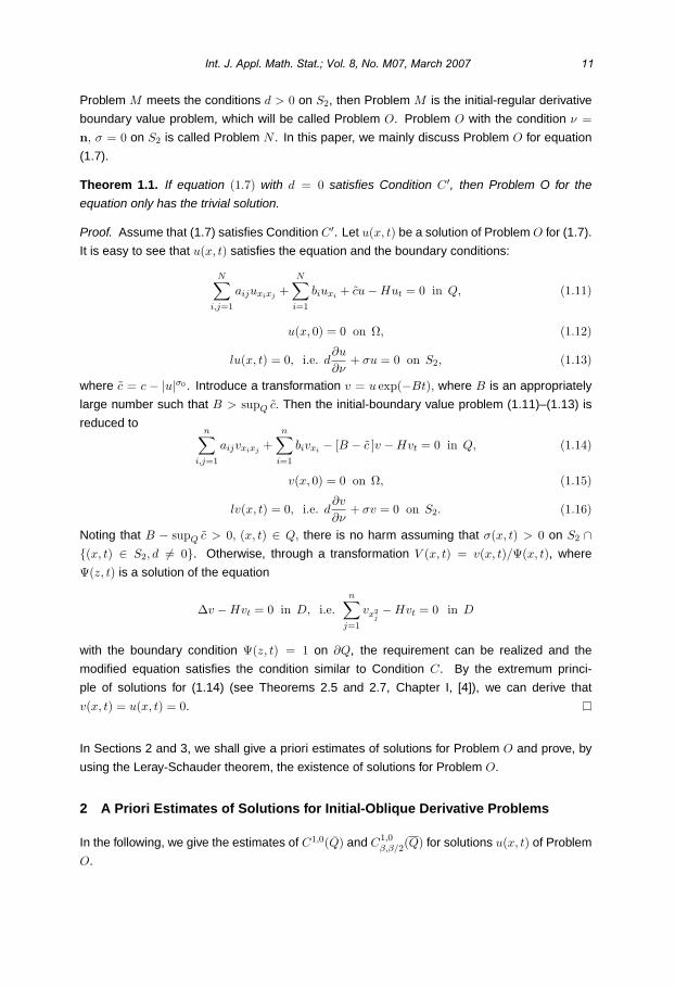
Theorem 1.1. If equation (1.7) with d = 0 satisfies Condition C ′, then Problem O for the

equation only has the trivial solution.

Proof. Assume that (1.7) satisfies Condition C ′. Let u(x, t) be a solution of Problem O for (1.7).

It is easy to see that u(x, t) satisfies the equation and the boundary conditions:

N∑i,j=1

aijuxixj +N∑

i=1

biuxi + cu − Hut = 0 in Q, (1.11)

u(x, 0) = 0 on Ω, (1.12)

lu(x, t) = 0, i.e. d∂u

∂ν+ σu = 0 on S2, (1.13)

where c = c − |u|σ0 . Introduce a transformation v = u exp(−Bt), where B is an appropriately

large number such that B > supQ c. Then the initial-boundary value problem (1.11)–(1.13) is

reduced ton∑

i,j=1

aijvxixj +n∑

i=1

bivxi − [B − c ]v − Hvt = 0 in Q, (1.14)

v(x, 0) = 0 on Ω, (1.15)

lv(x, t) = 0, i.e. d∂v

∂ν+ σv = 0 on S2. (1.16)

Noting that B − supQ c > 0, (x, t) ∈ Q, there is no harm assuming that σ(x, t) > 0 on S2 ∩(x, t) ∈ S2, d = 0. Otherwise, through a transformation V (x, t) = v(x, t)/Ψ(x, t), where

Ψ(z, t) is a solution of the equation

∆v − Hvt = 0 in D, i.e.n∑

j=1

vx2j− Hvt = 0 in D

with the boundary condition Ψ(z, t) = 1 on ∂Q, the requirement can be realized and the

modified equation satisfies the condition similar to Condition C. By the extremum princi-

ple of solutions for (1.14) (see Theorems 2.5 and 2.7, Chapter I, [4]), we can derive that

v(x, t) = u(x, t) = 0.

In Sections 2 and 3, we shall give a priori estimates of solutions for Problem O and prove, by

using the Leray-Schauder theorem, the existence of solutions for Problem O.

2 A Priori Estimates of Solutions for Initial-Oblique Derivative Problems

In the following, we give the estimates of C1,0(Q) and C1,0β,β/2(Q) for solutions u(x, t) of Problem

O.


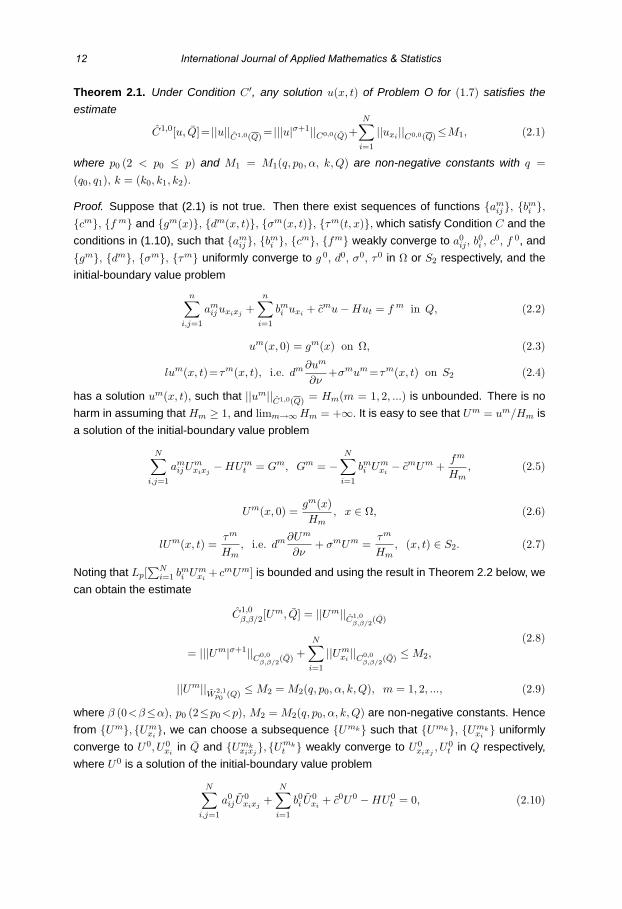
Theorem 2.1. Under Condition C ′, any solution u(x, t) of Problem O for (1.7) satisfies the

estimate

C1,0[u, Q]= ||u||C1,0(Q) = |||u|σ+1||C0,0(Q)+N∑

i=1

||uxi ||C0,0(Q)≤M1, (2.1)

where p0 (2 < p0 ≤ p) and M1 = M1(q, p0, α, k,Q) are non-negative constants with q =(q0, q1), k = (k0, k1, k2).

Proof. Suppose that (2.1) is not true. Then there exist sequences of functions amij , bm

i ,cm, f m and gm(x), dm(x, t), σm(x, t), τm(t, x), which satisfy Condition C and the

conditions in (1.10), such that amij , bm

i , cm, fm weakly converge to a0ij , b0

i , c0, f 0, and

gm, dm, σm, τm uniformly converge to g 0, d0, σ0, τ0 in Ω or S2 respectively, and the

initial-boundary value problem

n∑i,j=1

amij uxixj +

n∑i=1

bmi uxi + cmu − Hut = f m in Q, (2.2)

um(x, 0) = gm(x) on Ω, (2.3)

lum(x, t)=τm(x, t), i.e. dm ∂um

∂ν+σmum =τm(x, t) on S2 (2.4)

has a solution um(x, t), such that ||um||C1,0(Q) = Hm(m = 1, 2, ...) is unbounded. There is no

harm in assuming that Hm ≥ 1, and limm→∞ Hm = +∞. It is easy to see that Um = um/Hm is

a solution of the initial-boundary value problem

N∑i,j=1

amij U

mxixj

− HUmt = Gm, Gm = −

N∑i=1

bmi Um

xi− cmUm +

fm

Hm, (2.5)

Um(x, 0) =gm(x)Hm

, x ∈ Ω, (2.6)

lUm(x, t) =τm

Hm, i.e. dm ∂Um

∂ν+ σmUm =

τm

Hm, (x, t) ∈ S2. (2.7)

Noting that Lp[∑N

i=1 bmi Um

xi+ cmUm] is bounded and using the result in Theorem 2.2 below, we

can obtain the estimate

C1,0β,β/2[U

m, Q] = ||Um||C1,0

β,β/2(Q)

= |||Um|σ+1||C0,0

β,β/2(Q)

+N∑

i=1

||Umxi||

C0,0β,β/2

(Q)≤ M2,

(2.8)

||Um||W 2,1

p0(Q)

≤ M2 = M2(q, p0, α, k,Q), m = 1, 2, ..., (2.9)

where β (0<β≤α), p0 (2≤p0 <p), M2 = M2(q, p0, α, k,Q) are non-negative constants. Hence

from Um, Umxi, we can choose a subsequence Umk such that Umk, Umk

xi uniformly

converge to U0, U0xi

in Q and Umkxixj

, Umkt weakly converge to U0

xixj, U0

t in Q respectively,

where U0 is a solution of the initial-boundary value problem

N∑i,j=1

a0ijU

0xixj

+N∑

i=1

b0i U

0xi

+ c0U0 − HU0t = 0, (2.10)


U0(x, 0) = 0, x ∈ Ω, (2.11)

lU0(x, t) = 0, i.e. d∂U0

∂ν+ σU0 = 0, (x, t) ∈ S2. (2.12)

According to Theorem 1.1, we know U0(x, t) = 0, (x, t) ∈ Q. However, from ||Um||C1,0(Q) = 1,

there exists a point (x∗, t∗)∈Q, such that |U0(x∗, t∗)|+∑Ni=1 |U0

xi(x∗, t∗)| > 0. This contradiction

proves that (2.1) is true.

Theorem 2.2. Under the same condition in Theorem 2.1, any solution u(x, t) of Problem O

satisfies the estimates

||u||C1,0

β,β/2(Q)

≤ M3 = M3(q, p0, α, k,Q), (2.13)

||u||W 2,1

p0(Q)

≤ M4 = M4(q, p0, α, k,Q), (2.14)

where β (0 < β ≤ α), p0 (2 ≤ p0 ≤ p),Mj (j = 3, 4) are non-negative constants.

Proof. First of all, we find a solution u(x, t) of the equation

∆u − Hut = 0 (2.15)

with the initial-boundary conditions (1.8) and (1.9), which satisfies the estimate

||u||C2,1(Q) ≤ M5 = M5(q, p0, α, k,Q) (2.16)

(see Chapter III of [4] and [2]). Thus the function

u(x, t) = u(x, t) − u(x, t) (2.17)

is a solution of the equation

Lu =N∑

i,j=1

aij uxixj +N∑

i=1

biuxi + cu − Hut = f , (2.18)

u(x, 0) = 0, x ∈ Ω, (2.19)

lu(x, t) = 0, (x, t) ∈ S2, (2.20)

where f = f − Lu. Introduce a local coordinate system x = x(ξ) on the neighborhood G of a

surface S0 ∈ ∂Ω as follows:

xi = hi(ξ1, ..., ξN−1)ξN + gi(ξ1, ..., ξN−1), i = 1, ..., N, (2.21)

where ξN = 0 is just the surface S0 : xi = gi(ξ1, ..., ξN−1) (i = 1, ..., N), and

hi(ξ) =di(x)d(x)

∣∣∣∣xi=gi(ξ)

, i = 1, ..., N, d2(x) =N∑

i=1

d2i (x).

Then the boundary condition (2.20) can be reduced to the form

∂u

∂ξN+ σ = 0 on ξN = 0, (2.22)


where u = u[x(ξ), t], σ = σ[x(ξ), t]. Secondly, we find a solution v(x, t) of Problem N for

equation (2.15) with the boundary condition

∂v

∂ξN= σ on ξN = 0, (2.23)

which satisfies the estimate

||v||C2,1(Q) ≤ M6 = M6(q, p0, α, k,Q) < ∞. (2.24)

It is seen that the function

V (x, t) = uev(x,t) (2.25)

is a solution of the initial-boundary value problem

N∑i,j=1

aijVξiξj+

N∑i=1

biVxi + cV − HVt = f , (2.26)

∂V

∂ξN= 0, ξN = 0. (2.27)

On the basis of Theorem 3.3, Chapter III, [4], we can derive the following estimates of V (ξ, t):

||V ||C1,0

β,β/2(Q)

≤ M7 = M7(q, p0, α, k,Q), (2.28)

||V ||W 2,1

p0(Q)

≤ M8 = M8(q, p0, α, k,Q), (2.29)

where β (0<β≤α), p0 (2≤p0 <p),Mj (j = 7, 8) are non-negative constants. Combining (2.16),(2.24), (2.28) and (2.29), the estimates (2.13) and (2.14) are obtained.

By using the similar method as in the proof of Theorem 2.1, we can prove the following theorem.

Theorem 2.3. Suppose that equation (1.7) satisfies Condition C ′. Then any solution u(x, t) of

Problem O satisfies the estimates

C1,0β,β/2[u, Q] = ||u||

C1,0β,β/2

(Q)≤ M9(k1 + k2), (2.30)

||u||W 2,1

p0(Q)

≤ M10(k1 + k2), (2.31)

where β(0 < β ≤ α), p0 (2 ≤ p0 < p),Mj = Mj(q, p0, α, k0, Q) (j = 9, 10) are non-negative

constants.

3 Solvability of Initial-Oblique Derivative Problems for Parabolic Equations

We first consider a special equation of (1.7):

∆u − Hut = gm(x, t, u,Dxu, D2xu),

gm =∆u−N∑

i,j=1

aijmuxixj −N∑

i=1

bimu−cmu+fm in Q,(3.1)


with ∆u =∑N

i=1 ∂2u/∂x2i , Λ = 2 infQ

∑Ni=1 aii/(2N − 1), and the coefficients

aijm =

⎧⎨⎩

aij/Λ,

δij/Λ,bim =

⎧⎨⎩

bi/Λ,

0,i, j = 1, ..., N,

cm =

⎧⎨⎩

c/Λ,

0,H =

⎧⎨⎩

1/Λ,

1/Λ,fm =

⎧⎨⎩

f/Λ

0

in Qm,

in RN × I\Qm,

(3.2)

where Qm = (x, t) ∈ Q |dist((x, t), ∂Q) ≥ 1/m for a positive integer m, δii = 1, δij = 0 (i =j, i, j = 1, ..., N). In particular, the linear case of equation (3.1) can be written as

∆u−HuΛt =gm(x, t, u,Dxu, D2xu), gm =

N∑i,j=1

[δij−aijm(x, t)]uxixj

−N∑

i=1

bim(x, t)uxi−cm(x, t)u+fm(x, t) in Q. (3.3)

In the following, we will give the representation of solutions of Problem O for equation (3.1).

Theorem 3.1. Under Condition C ′, if u(x, t) is a solution of Problem O for equation (3.1), then

u(x, t) can be expressed in the form

u(x, t)=U(x, t)+V (x, t)=U(x, t)+v0(x, t)+v(x, t),

v(x, t) = Hρ =∫

Q0

G(x, t, ζ, τ)ρ(ζ, τ)dσζdτ,

G =

⎧⎨⎩

[Λ(t − τ)]−N/2 exp[|x − ζ|2/4Λ(t − τ)], t > τ,

0, t ≤ τ, except t − τ = |x − ζ| = 0.

(3.4)

In (3.4), ρ(x, t) = ∆u − Hut = ∆u − uΛt = gm. V (x, t) is a solution of Problem D for (3.1) in

Q0 = Ω0 × I with the initial-boundary condition V (x, t) = 0 on ∂Q0, where Ω0 = |x| < R for

a large number R such that Ω0 ⊃ Ω. U(x, t) is a solution of Problem P for LU = ∆U −UΛt = 0in Q with the initial-boundary condition (3.12) − (3.13) below. V (x, t) and U(x, t) satisfy the

estimatesC1,0

β,β/2[U,Q] + ||U ||W 2,1

2 (Q)≤ M11,

C1,0β,β/2[V , Q0] + ||V ||

W 2,12 (Q0)

≤ M12,(3.5)

where β(0 < β ≤ α), Mj = Mj(q, p0, α, k,Qm) (j = 11, 12) are non-negative constants, q =(q0, q1), k = (k0, k1, k2).

Proof. It is easy to see that the solution u(x, t) of Problem O for equation (3.1) can be ex-

pressed by the form (3.4). Since aijm = 0 (i = j), bim = 0, cm = 0, fm(x, t) = 0 in RN ×I\Qm and V (x, t) is a solution of Problem D for (3.1) in Q0, we can see that V (x, t) in

Q2m = Q\Q2m satisfies the estimate

C2,1[V (x, t), Q2m] ≤ M13 = M13(q, p0, α, k,Qm).

On the basis of Theorem 2.3, we can see that U(x, t) satisfies the first estimate in (3.5), and

then V (x, t) satisfies the second estimate in (3.5).


Theorem 3.2. If equation (1.7) satisfies Condition C ′, then Problem O for (3.3) has a solution

u(x, t).

Proof. In order to prove the existence of solutions of Problem O for the nonlinear equation (3.1)

by using the Larey-Schauder theorem, we introduce the equation with the parameter h ∈ [0, 1]

∆u − uΛt = hgm(x, t, u,Dxu, D2xu) in Q. (3.6)

Denote by BM a bounded open set in the Banach space B = W 2,12 (Q) = C1,0

β,β/2(Q)∩W 2,12 (Q)

for 0 < β ≤ α, the elements of which are real functions V (x, t) satisfying the inequalities

||V ||W 2,1

2 (Q)= C1,0

β,β/2[V, Q] + ||V ||W 2,1

2 (Q)< M14 = M3 + M4 + 1, (3.7)

in which W 2,12 (Q) = W 2,0

2 (Q) ∩ W 0,12 (Q), M3,M4 are the non-negative constants as stated in

(2.13) and (2.14). We choose any function V (x, t) ∈ BM and substitute it into the appropriate

positions on the right hand side of (3.6), and then we make an integral v(x, t) = Hρ as follows:

v(x, t) = Hρ, ρ(x, t) = ∆V − VΛt. (3.8)

Next we find a solution v(x, t) of the initial-boundary value problem in Q0:

∆v0 − v0Λt = 0 on Q0, (3.9)

v(x, t) = −v(x, t) on ∂Q0, (3.10)

and denote by V (x, t) = v(x, t) + v(x, t) the solution of the corresponding Problem D in Q0.

Moreover, on the basis of the result in Chapter III of [4] and [2], we can find a solution U(x, t)of the corresponding Problem O in Q:

∆U − UΛt = 0 on Q, (3.11)

U(x, 0) = g(x) − V (x, 0) on Ω, (3.12)

∂U

∂ν+ σ(x, t)U = τ(x, t) − ∂V

∂ν+ σ(x, t)V on S2. (3.13)

Now we discuss the equation

∆V − VΛt = hgm(x, t, u,Dxu, D2xU + D2

xV ), 0 ≤ h ≤ 1, (3.14)

where u = U + V . By Condition C, applying the principle of contracting mapping, we can find

a unique solution V (x, t) of Problem D for equation (3.14) in Q0 satisfying the initial-boundary

condition

V (x, t) = 0 on ∂Q0. (3.15)

Here we mention that due to Section 2, Chapter I, [4] and the result in [3], we can use the

principle of contracting mapping. If we do not have the conditions and results, it is impossible

to use the principle. Set u(x, t) = U(x, t) + V (x, t), where the relation between U and V is the

same as that between u and V , and denote by V = S(V , h) and u = S1(V , h) (0 ≤ h ≤ 1) the


mappings from V onto V and u respectively. Furthermore, if V (x, t) is a solution of Problem D

in Q0 for the equation

∆V − VΛt = hgm(x, t, u,Dxu, D2x(U + V )), 0 ≤ h ≤ 1, (3.16)

where u = S1(V, h), then from Theorem 3.1, the solution V (x, t) of Problem D for (3.16) satis-

fies the estimate (3.7), and consequently V (x, t) ∈ BM . Set B0 = BM × [0, 1]. In the following,

we shall verify that the mapping V = S(V , h) satisfies the three conditions of Leray-Schauder

theorem.

1) For every h ∈ [0, 1], V = S(V , h) continuously maps the Banach space B into itself, and is

completely continuous on BM . Besides, for every function V (x, t) ∈ BM , S(V , h) is uniformly

continuous with respect to h ∈ [0, 1].

In fact, we arbitrarily choose Vl(x, t) ∈ BM (l = 1, 2, ...). It is clear that from Vl(x, t) there

exists a subsequence Vlk(x, t) such that Vlk(x, t), Vlkxi(x, t) (i = 1, ..., N) and corre-

sponding functions Ulk(x, t), Ulkxi(x, t), ulk(x, t), ulkxi

(x, t) (i = 1, ..., N) uniformly

converge to V0(x, t), V0xi(x, t), U0(x, t), U0xi(x, t), u0(x, t), u0xi(x, t) (i = 1, ..., N) in Q0, Q re-

spectively, in which ulk = S1(Vlk , h), u0 = S1(V0, h). We can find a solution V0(x, t) of Problem

D for the equation

∆V0−V0Λt =hgm(x, t, u0, Dxu0, D2xU0 + D2

xV0), 0≤h≤1 in Q0. (3.17)

From Vlk = S(Vlk , h) and V0 = S(V0, h), we have

∆(Vlk − V0) − (Vlk − V0)Λt = h[gm(x, t, ulk , Dxulk , D2xUlk + D2

xVlk)

−gm(x, t, ulk , Dxulk , D2xUlk + D2

xV0) + Clk(x, t)], 0 ≤ h ≤ 1,

whereClk(z, t) = gm(x, t, ulk , Dxulk , D2

xUlk + D2xV0)

−gm(x, t, u0, Dxu0, D2xU0 + D2

xV0), (x, t) ∈ Q0.

Later we shall prove that

L2[Clk(x, t), Q0] → 0 as k → ∞. (3.18)

Moreover, according to Theorem 2.3, we can derive that

||Vlk − V0||W 2,12 (Q0)

≤ M15L2[Clk , Q0],

where M15 = M15(q, p0, α, k0, Qm) is a non-negative constant, and hence ||Vlk −V0||W 2,12 (Q0)

→0 as k → ∞. Thus from Vlk(x, t) − V0(x, t), there exists a subsequence, denoted, for con-

venience, by Vlk(x, t) − V0(x, t), such that ||Vlk(x, t) − V0(x, t)||W 2,1

2 (Q0)= C1,0

β,β/2[Vlk(x, t)−V0(x, t), Q0] + ||Vlk(x, t) − V0(x, t)||

W 2,12 (Q0)

→ 0 as k → ∞. From this we can obtain that

the corresponding subsequence ulk(x, t) − u0(x, t) = S1(Vlk , h) − S1(V0, h) possesses

the property: ||ulk(x, t) − u0(x, t)||W 2,1

2 (Q)→ 0 as k → ∞. This shows the complete conti-

nuity of V = S(V , h) (0 ≤ h ≤ 1) in BM . By using the similar method, we can prove that


V = S(V , h) (0 ≤ h ≤ 1) continuously maps BM into B, and V = S(V , h) is uniformly continu-

ous with respect to h ∈ [0, 1] for V ∈ BM .

2) For h = 0, from Theorem 2.2 and (3.7), it is clear that V = S(V , 0) ∈ BM .

3) From Theorem 2.2 and (3.7), we see that V = S(V , h)(0 ≤ h ≤ 1) does not have a solution

u(x, t) on the boundary ∂BM = BM\BM .

Hence by the Leray-Schauder theorem, we know that Problem D0 for equation (3.6) with h=1has a solution V (z, t) ∈ BM , and then Problem O of equation (3.6) with h = 1, i.e. (3.1) has a

solution u(x, t)=S1(V , h)=U(x, t)+V (x, t)=U(x, t)+v(x, t)+v(x, t) ∈ B.

Finally, we verify (3.18). In fact, by Condition C ′ and the above discussion, we can choose, from

Clk(x, t), a subsequence denoted by Clk(x, t) again, such that Clk(x, t) converges 0 for

almost every point in Q0. Hence for two sufficiently small positive numbers ε1, ε2, there exist a

subset Q∗ in Q0 and a positive number K0, such that mes Q∗ < ε1 and |Clk | < ε2, (x, t) ∈ Q0\Q∗as k > K0. According to the Holder inequality and Minkowski inequality, we have

L2[Clk , Q∗] + L2[Clk , Q0\Q∗]

≤ Lp1 [Clk , D∗]Lp2 [1, D∗] + ε2 (mes Q0)1/2

≤ ε1/p2

1 M16 + ε2(mes Q0)1/2 = ε,

where p2 is a sufficiently large positive constant, p1 = 2p2/(p2 − 2) is a positive constant near

2, and M16 = sup1≤k<∞ Lp1 [Clk , Q∗] is a constant. Provided that ε1, ε2 are small enough, ε can

be sufficiently small. This shows that (3.18) is true.

Theorem 3.3. Under the same condition in Theorem 3.2, Problem O for equation (1.7) has a

solution.

Proof. By Theorems 2.2 and 3.2, Problem O for equation (3.1) possesses a solution um(x, t)that satisfies the estimates (2.30) and (2.31)(m = 1, 2, ...). Thus, we can choose a subse-

quence umk(x, t), such that umk

(x, t), umkxi(x, t) (i = 1, ..., N) in Q uniformly converge

to u0(x, t), u0xi(x, t) (i = 1, ..., N), respectively. Obviously, u0(x, t) satisfies the initial-boundary

conditions of Problem O. On the basis of principle of compactness of solutions for equation

(3.1) (see Theorem 4.6, Chapter I, [4]), we can see that u0(x, t) is a solution of Problem O for

(1.7).

References

[1] Y. A. Alkhutov and I. T. Mamedov, The first boundary value problem for nondivergence

second order parabolic equations with discontinuous coefficients, Math. USSR Sbornik

59, 471–495(1988).

[2] O. A. Ladyzhenskaja, V. A. Solonnikov, and N. N. Uraltseva, Linear and quasilinear equa-

tions of parabolic type, (Amer. Math. Soc., Providence, RI, 1968).


[3] G. C. Wen, Linear and nonlinear parabolic complex equations, (World Scientific, Singa-

pore, 1999).

[4] G. C. Wen, Initial-boundary value problems for nonlinear parabolic equations in higher

dimensional domains, (Science Press, Beijing, 2002).


Some solutions of generalized Rassias’s equation

Anvar Hasanov

Institute of Mathematics, Uzbek Academy of Sciences, 29, F. Hodjaev street, Tashkent 700125, Uzbekistan

E-mail: [email protected], [email protected]

Abstract

In the field of 3 , , : 0, 0, 0x y z x y z the generalized Rassias’s equation

0,m k n k n m

xx yy zzR u y z u x z u x y u

, , 0,m n k const is considered. By means of a change of variables the generalized

Rassias’s equation to be reduced to a system of hypergeometric equations for the function of Lauricella of three variables. Eight linearly independent particular solutions of the system of hypergeometric equations are found. Properties of found particular solutions are studied by virtue of decomposition of the hypergeometric function of Lauricella.

2000 Mathematics Subject Classification. 35L80

Key Words and Phrases. Degenerating hyperbolic equation, particular solution, singular partial differential equation.

1 INTRODUCTION

In paper [1] studies the equation

, , , , ,xx yy zzR u k z u u u x y z u f x y z (1.1)

0, 0,

0, 0,

k z for z

k z for z

in a simply connected bounder domain 3D . There are some works, for example:

[2-4] in which the some modifications of equation (1.1) are considered. We shall

consider the equation (1.1) in the case of when 1, , , , , 0k z x y z f x y z and

we shall construct particular solutions of the equation (1.1). Also, we study the

generalized Rassias’s equation which degenerates in each hyper plane of the

space 3 , , : 0, 0, 0x y z x y z . For the generalized Rassias’s equation, we

find eight linearly independent particular solutions. Using decompositions of


hypergeometric function of Lauricella in a series on products of hypergeometric

function of Gauss, we investigate behavior of the found particular solutions at 0 .

2. PARTICULAR SOLUTIONS Of RASSIAS’S EQUATION

In the domain, 3 , , : , , ,x y z x y z we shall

consider the equation

0.xx yy zzL u u u u (2.1)

The solution of the equation (2.1) we shall search in the form of

,u (2.2)

Where is unknown function and

2 2 2

0 0 0 .x x y y z z (2.3)

Let’s calculate derivatives

2 2 2

, , ,

, , .

x x y y z z

xx x xx yy y yy zz z zz

u u u

u u u (2.4)

Substituting (2.4) in to the (2.1) we get

2 2 2 0.x y z xx yy zz (2.5)

We calculate derivatives

0 0 02 , 2 , 2 , 2, 2, 2.x y z xx yy zzx x y y z z (2.6)

Substituting (2.6) in to the equation (2.5), we have

2 3 0. (2.7)

The equations (2.7) has the following solution

1

21 2 1 2, , .c c c c const (2.8)

3. SOME PARTICULAR SOLUTIONS OF GENERALIZED RASSIAS’S EQUATION

We consider in the domain 3 , , : 0, 0, 0x y z x y z a generalized

Rassias’s equation

0, , , 0m k n k n m

xx yy zzR u y z u x z u x y u m n k const . (3.1)

The solution of the equation (3.1) we search in the form of

, ,u P , (3.2)


where

1

2 ,P (3.3)

31 2, , , , , ,2 2 2 2 2 2

n m k

n m k (3.4)

2 2 2

2 2 2 2 2 21 2 2 2 2 2 2

0 0 0

2

3

2 2 2 2 2 2.

2 2 2 2 2 2

n n m m k k

x x y y z zn n m m k k

(3.5)

Substituting (3.2) in to the (3.1), we have

1 2 3 1 2 3 1 2 3 0,A A A B B B C C C D (3.6)

where

2 2 2

1 ,m k n k n m

x y zA P y z x z x y

2 2 2

2 ,m k n k n m


2 2 2

3 ,m k n k n m


1 2 ,m k n k n m

x x y y z zB P y z x z x y

2 2 ,m k n k n m


3 2 ,m k n k n m


1 2 2 2 ,m k n k n m m k n k n m

x x y y z z xx yy zzC y z P x z P x y P y z P x z P x y P

2 2 2 2 ,m k n k n m m k n k n m


3 2 2 2 ,m k n k n m m k n k n m


.m k n k n m

xx yy zzD y z P x z P x y P

After elementary evaluations, we find

2 2

2 21 0

41 ,

n nn m kPx y zA x x (3.7)

2 2

2 22 0

41 ,

m mn m kPx y zA y y (3.8)

2 2

2 23 0

41 ,

k kn m kPx y zA z z (3.9)


2 2 2 2

2 2 2 21 0 0

4 4,

m m n nn m k n m kPx y z Px y zB y y x x (3.10)

2 2 2 2

2 2 2 22 0 0

4 4,

n n k kn m k n m kPx y z Px y zB x x z z (3.11)

2 2 2 2

2 2 2 23 0 0

4 4,

m m k kn m k n m kPx y z Px y zB y y z z (3.12)

2 2

2 21 0

2 2 2 2

2 2 2 20 0

4 12 1

2

4 4,

n nn m k

m m k kn m k n m k

Px y zC x x

Px y z Px y zy y z z

(3.13)

2 2 2 2

2 2 2 22 0 0

2 2

2 20

4 4 12 1

2

4,

n n m mn m k n m k

k kn m k

Px y z Px y zC x x y y

Px y zz z

(3.14)

2 2 2 2

2 2 2 23 0 0

2 2

2 20

4 4

4 12 1 ,

2

n n k kn m k n m k

m mn m k

Px y z Px y zC x x y y

Px y zz z

(3.15)

2 2 2 2

2 2 2 20 0

2 2

2 20

4 1 4 1

2 2

4 1.

2

n n m mn m k n m k

k kn m k

Px y z Px y zD x x y y

Px y zz z

(3.16)

Substituting (3.7) - (3.16) in to the (3.6) we get

2 2

2 20

4

11 2 1

2

1

2

n nn m kPx y zx x

2 2

2 20

4

11 2 1

2

1

2

m mn m kPx y zy y

(3.17)


2 2

2 20

4

11 2 1

20.

1

2

k kn m kPx y zz z

Solutions of the system of hypergeometric equations

11 2 1

2

10

2

11 2 1

2

10

2

11 2 1

2

10,

2

(3.18)

also satisfies to the equation (3.17). The system of hypergeometric equations (3.18)

has eight linearly independent solutions ([5], p. 117-118)

3

1

1, , ; , , ;2 , 2 ,2 ; , , ,

2AF (3.19)

31 2

2

3, , ;1 , , ;2 2 ,2 ,2 ; , , ,

2AF (3.20)

31 2

3

3, , ; ,1 , ;2 , 2 2 ,2 ; , , ,

2AF (3.21)

31 2

4

3, , ; , ,1 ;2 ,2 ,2 2 ; , , ,

2AF (3.22)

31 2 1 2

5

5, , ;1 ,1 , ;2 2 ,2 2 ,2 ; , , ,

2AF (3.23)

31 2 1 2

6

5, , ;1 , ,1 ;2 2 ,2 ,2 2 ; , , ,

2AF (3.24)

31 2 1 2

7

5, , ; ,1 ,1 ;2 ,2 2 ,2 2 ; , , ,

2AF (3.25)


1 2 1 2 1 2

8

3

, ,

7;1 ,1 ,1 ;2 2 ,2 2 ,2 2 ; , , .2

AF (3.26)

Substituting the found solutions (3.19) - (3.26) in to the (3.2), finally we define

particular solutions of (3.1)

132

1 0 0 0 1

1, , ; , , ; , , ;2 , 2 , 2 ; , , ,

2Au x y z x y z F (3.27)

3

22 0 0 0 2 0

3

, , ; , ,

3;1 , , ;2 2 ,2 ,2 ; , , ,2

A

u x y z x y z xx

F

(3.28)

3

23 0 0 0 3 0

3

, , ; , ,

3; ,1 , ;2 , 2 2 ,2 ; , , ,2

A

u x y z x y z yy

F

(3.29)

3

24 0 0 0 4 0

3

, , ; , ,

3; , ,1 ;2 ,2 ,2 2 ; , , ,2

A

u x y z x y z zz

F

(3.30)

5

25 0 0 0 5 0 0

3

, , ; , ,

5;1 ,1 , ;2 2 ,2 2 ,2 ; , , ,2

A

u x y z x y z xx yy

F

(3.31)

5

26 0 0 0 6 0 0

3

, , ; , ,

5;1 , ,1 ;2 2 ,2 ,2 2 ; , , ,2

A

u x y z x y z xx zz

F

(3.32)

5

27 0 0 0 7 0 0

3

, , ; , ,

5; ,1 ,1 ;2 ,2 2 ,2 2 ; , , ,2

A

u x y z x y z yy zz

F

(3.33)

7

28 0 0 0 8 0 0 0

3

, , ; , ,

7;1 ,1 ,1 ;2 2 ,2 2 ,2 2 ; , , ,2

A

u x y z x y z xyzx y z

F

(3.34)

where , 1, 2,...,8i i are constants and hypergeometric function of Lauricella looks

like [5]


1 2 33

1 2 3 1 2 3

, , 0 1 2 3

; , , ; , , ; , , ,! ! !

i j l i j l i j l

A

i j l i j l

a b b bF a b b b c c c x y z x y z

c c c i j l (3.35)

1 1 2 2 3 331 2

3 1 2 3

1 2 3 1 2 3

1 2 3 1 1 2 2 3 3

1 1 11 1 111 1

1 2 3 1 2 3 1 2 3 1 2 3

0 0 0

; , , ; , , ; , ,

1 1 1 1 ,

A

c b c b c b abb b

c c cF a b b b c c c x y z

b b b c b c b c b

t t t t t t xt yt zt dt dt dt

(3.36)

1 1 2 2 3 3Re Re 0,Re Re 0,Re Re 0.c b c b c b

Here, and in what follows, / denotes the Pochhammer symbol

(or the shifted factorial) for all admissible (real or complex) values of and .

4. PROPERTIES OF PARTICULAR SOLUTIONS OF GENERALIZED RASSIAS’S EQUATION

We study properties of particular solutions (3.27) - (3.34). It is not difficult to

prove that, the following identities

1 1 1 2 2 200 0 00 0

0, 0, 0, 0, 0, 0,x

x z zy y

u u u u u ux y z y z

(4.1)

3 3 3 4 4 40 00 0 0 0

0, 0, 0, 0, 0, 0,y z

x z x y

u u u u u ux z x y

(4.2)

5 5 5 6 6 60 0 0 00 0

0, 0, 0, 0, 0, 0,x y x z

z y

u u u u u uz y

(4.3)

7 7 7 8 8 80 0 0 0 00

0, 0, 0, 0, 0, 0,y z x y z

x

u u u u u ux

(4.4)

are true.

We investigate behavior of particular solutions (3.27) - (3.34) at 0 . For

this aim we use decomposition ([7], p. 117, (14))

3

1 2 3 1 2 3

1 2 3

, , 0 1 2 3

2 1 1 1 2 1 2 2

2 1 3 3

; , , ; , , ; , ,

! ! !

, ; ; , ; ;

, ; ; ,

A

l m l n m nl m n l m l n m n

l m n l m l n m n

F a b b b c c c x y z

a b b bx y z

c c c l m n

F a l m b l m c l m x F a l m n b l n c l n y

F a l m n b m n c m n z

(4.5)

where


2 1

0

, ; ; ,!

mm m

m m

a bF a b c x x

c m

is a hypergeometric function of Gauss [5, 6]. By virtue of decomposition (4.5), the

particular solution (3.27) can be written as

1

21 0 0 0 1

31 2

, , 0

12 1

2 1

, , ; , ,

1

21 1 1

2 2 2 ! ! !

1, ;2 ;1

2

1, ;2

2

m nl m l nl m l n m nl m n

l m n l m l n m n

u x y z x y z

l m n

F l m l m l m

F l m n l n 2

32 1

;1

1, ;2 ;1 .

2

l n

F l m n m n m n

(4.6)

We use the following formulae for a hypergeometric function of Gauss [6]

2 1 2 1, ; ; 1 , ; ; .1

b xF a b c x x F c a b c

x

Then equality (4.6) will have the following form

1

21 0 0 0 1 1 2 3 1 2 3, , ; , , , , , ,u x y z x y z f (4.7)

where

1 2 3

, , 0 1 2 3

2 1

1

2 1

2

2 1

, , ,

1

21 1 1

2 2 2 ! ! !

1, ;2 ;12

1, ;2 ;1

2

m nl m l nl m l n m n

l m n

l m n l m l n m n

f

l m n

F l m l m

F m l n l n

F3

1, ;2 ;1 .

2l m n m n

(4.8)

By virtue of equality

2 1 , ; ; , 0, 1, 2,...,Re 0,c c a b

F a b c x c c a bc a c b

(4.9)

we have


2 1

1 0

1, ;2 ;12

12 2

2,

1 1

2 2

l m

l m

F l m l m

(4.10)

2 1

2 0

1, ;2 ;1

2

1122

22,

1 1

2 2

l nm

l m n

F m l n l n

(4.11)

2 1

3 0

1, ;2 ;1

2

1122

22.

1 1

2 2

m nl

l m n

F l m n m n

(4.12)

Substituting (4.10) - (4.12) into the (4.8) we have

1 2 3

3

, , 0

0, , ,

1 1 12 2 2

2 2 2

1

2

1 1

2 2.

1 1! ! !

2 2

l m l n m nm l

l m n

l m n l m

f

l m n

(4.13)

It is easy to calculate, that

, , 0

2

1 1

2 2

1 1! ! !

2 2

1

2.

1 1 1

2 2 2

l m l n m nm l

l m n

l m n l m

l m

l m n

(4.14)


Substituting (4.14) in to (4.13), we have

1 2 3

2 2 20, , , .

1

2

f (4.15)

By virtue of equality (4.15) from (4.7) follows

1 0 0 0 1/ 2

1 2 3

, , ; , , , .c

u x y z x y z c const (4.16)

Expression (4.16) shows that, the particular solution 1 0 0 0, , ; , ,u x y z x y z is converted

to infinity with the order 1/ 2 at 0 . Similarly it is possible to be convinced, that

particular solutions 0 0 0, , ; , , , 2,3,...,8iu x y z x y z i are also converted to infinity with

the order 1/ 2 at 0 .

We study behavior of particular solutions (3.27) - (3.34) at . As at

arguments of the hypergeometric functions in the solution (3.27) - (3.34) are

converted to a zero, i.e. 0, 0, 0 particular solutions

0 0 0, , ; , , , 1, 2,...,8iu x y z x y z i are converted to zero of the order 1/ 2 .

ACKNOWLEDGEMENT

I am grateful to Professor John Michael Rassias for his kind interest during the preparation of this paper.

REFERENCES

[1] J. M. S. Rassias, 1979, The bi-hyperbolic degenerate boundary value problem in R3 Eleutheria, no. 2, 468-473.

[2] J. M. Rassias, 1980, A new bi-hyperbolic boundary value problem in the Euclidean space. Bull. Acad. Polon. Sci. Ser. Sci. Math. 28, no. 11-12, 565-568.

[3] J. M. Rassias, 1981, New uniqueness theorems, Bull. Acad. Polon. Sci. Ser. Sci. Math. 28 no. 11-12, 569-571.

[4] J. M. Rassias, 1982, The Bi-hyperbolic Degenerate Boundary Value Problem in R3, Discuss. Math., Vol. 5, 101-104.

[5] P. Appell and J. Kampe de Feriet, 1926, Fonctions Hypergeometriques et Hyperspheriques; Polynomes d’Hermite, Gauthier - Villars. Paris.

[6] A. Erdelyi, W. Magnus, F. Oberhettinger and F. G. Tricomi, 1953, Higher Transcendental Functions, Vol. I, McGraw-Hill Book Company, New York, Toronto and London.

[7] A. Hasanov and H. M. Srivastava, 2006, Some decomposition formulas associated with

the Lauricella function r

AF and other multiple hypergeometric functions, Appl. Math.

Lett. 19, no. 2, 113-121.


The solution of the Cauchy problem for generalized Euler-Poisson-Darboux equation

Anvar Hasanov

Institute of Mathematics, Uzbek Academy of Sciences, 29 F. Hodjaev Street, Tashkent 700125, Uzbekistan

E-mail: [email protected], [email protected]

Abstract.

In this paper in a characteristic triangle Cauchy problem for generalized Euler-Poisson-Darboux equation

, 0.L u u u u u

is considered. Function of Riemann, which expressed by Kummer’s function of three variables is constructed in an explicit form. By the method of Riemann for the hyperbolic equations, a solution of the Cauchy problem for generalized Euler-Poisson-Darboux equation expressed in an explicit form.

2000 Mathematics Subject Classification. primary 35Q05, 35L80; secondary 33C65.

Keywords: Generalized Euler-Poisson-Darboux equation, degenerating hyperbolic type equations, function of Riemann, a Cauchy problem, confluent hypergeometric functions of Kummer from three variables

1. INTRODUCTION

Many problems of gas dynamics can be reduced to boundary value problems for the mixed type degenerating equations. It is known that, the mixed type degenerating equations in a hyperbolic part of the domain reduced to the generalized Euler-Poisson-Darboux equation

, 0, 0 2 ,2 1,L u u u u u (1.1)

where , and are constant numbers. The Riemann function of generalized Euler-Poisson-Darboux equation (1.1) was not found. Hence, the Cauchy problem also not solved. Note, Euler-Poisson-Darboux equation

1 11 1 1 10, 0, 0, 1,L u u u u (1.2)

was considered in a work ([1], p. 57) and the Cauchy problem for the equation (1.2) was solved. In the papers [2-4] for the Euler-Poisson-Darboux equation (1.2) non-local boundary value problems in a characteristic triangle were solved. The method of Riemann also is applied to some equations of hyperbolic type [5-15].


In this paper, first we shall introduce two confluent hypergeometric functions from three variables. Further, for confluent hypergeometric functions formulas of an analytic continuation are proved. The function of Riemann for generalized Euler-Poisson-Darboux equation (1.1) by the help of introduced hypergeometric functions is build. Further, in a characteristic triangle with the help of Riemann’s function by a classical method we solve a Cauchy problem for generalized Euler-Poisson-Darboux equation (1.1). A solution of the Cauchy problem for generalized Euler-Poisson-Darboux equation (1.1) we shall construct in an explicit form.

2. CONSTRUCTIVE PROPERTIES OF GENERALIZED EULER-POISSON-DARBOUX EQUATION

We introduce a new function ,v , supposing

1 2, , .u v (2.1)

Then the equation (1.1) is reduced to

,1

1 10.L v v v v v (2.2)

Let's designate through ,u any solution of the equation (1.1). Then by virtue of equality

(2.1) we find the first constructive property

1 2

, ,1 .L u L u (2.3)

Similarly supposing

1 2, , ,u v (2.4)

we find the second constructive formula

1 2

, 1 , .L u L u (2.5)

Note, that constructive formulas (2.3) - (2.5) allow to solve some problems for various values of parameters , .

2. CONFLUENT HYPERGEOMETRIC FUNCTIONS OF KUMMER FROM THREE ARGUMENTS

Consider the system of hypergeometric equations ([16], p. 117)

1 1 1 1

2 2 2 2

3 3 3 3

1 1 0

1 1 0

1 1 0.

xx xy xz x

yy xy yz y

zz xz yz z

x x y z c a b x a b

y y x z c a b y a b

z z x y c a b z a b

(3.1)


The solution of the system of hypergeometric equations (3.1) is Lauricella’s hypergeometric function ([16], p. 114, (2))

1 2 3 1 2 33

1 2 3 1 2 3

, , 0

, , , , , ; ; , , ,! ! !

m n p m n p m n p

B

m n p m n p

a a a b b bF a a a b b b c x y z x y z

c m n p (3.2)

0, 1, 2,..., , , , 1 .c s x r y t z s r t

Using identity ([16], p. 124)

0 0 0

1 1 1lim lim lim 1m n p

m n p

, (3.3)

where / is a symbol of Pochhammer (or the shifted factorial). From

hypergeometric function (3.2), we find the following confluent hypergeometric functions of three variables

3

1 1 2 3 1 2 1 2 3 1 20

1 2 3 1 2

, , 0

1, , , , ; ; , , lim , , , , , ; ; , ,

,! ! !

B

m n p m n m n p

m n p m n p

B a a a b b c x y z F a a a b b c x y z

a a a b bx y z

c m n p

(3.4)

3 2

2 1 2 1 2 1 2 1 20

1 2 1 2

, , 0

1 1, , , ; ; , , lim , , , , , ; ; , ,

.! ! !

B

m n pm n m n

m n p m n p

B a a b b c x y z F a a b b c x y z

a a b bx y z

c m n p

(3.5)

The found hypergeometric functions 1B , 2B accordingly satisfy to the following systems of

hypergeometric equations

1 1 1 1

2 2 2 2

3

1 1 0

1 1 0

0,

xx xy xz x

yy xy yz y

zz xz yz z

x x y z c a b x a b

y y x z c a b y a b

z x y c z a

(3.6)

1 1 1 1

2 2 2 2

1 1 0

1 1 0

0.

xx xy xz x

yy xy yz y

zz xz yz z

x x y z c a b x a b

y y x z c a b y a b

z x y c

(3.7)

Confluent hypergeometric functions 1B , 2B have accordingly the following integral

representations


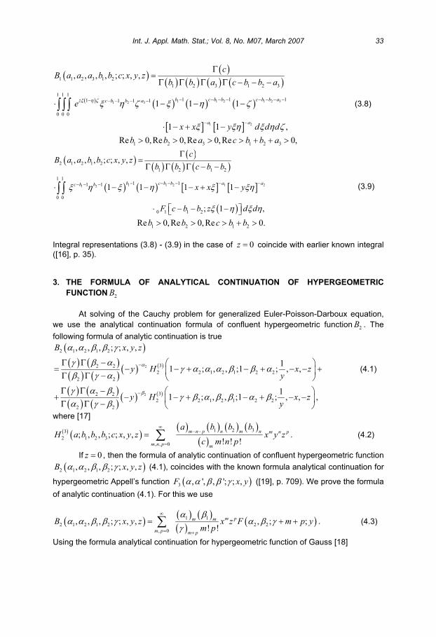
1 1 2 1 2 331 2

1 2

1 1 2 3 1 2

1 2 3 1 2 3

1 1 11 1 11 11 1

0 0 0

, , , , ; ; , ,

1 1 1

1 1 ,

b c b b c b b az ac b b

a a

cB a a a b b c x y z

b b a c b b a

e

x x y d d d

(3.8)

1 2 3 1 2 3Re 0,Re 0,Re 0,Re 0,b b a c b b a

1 21 1 21 2

2 1 2 1 2

1 2 1 2

1 11 11 1

0 0

0 1 1 2

, , , ; ; , ,

1 1 1 1

; 1 ,

a ab c b bc b b

cB a a b b c x y z

b b c b b

x x y

F c b b z d d

(3.9)

1 2 1 2Re 0,Re 0,Re 0.b b c b b

Integral representations (3.8) - (3.9) in the case of 0z coincide with earlier known integral ([16], p. 35).

3. THE FORMULA OF ANALYTICAL CONTINUATION OF HYPERGEOMETRIC

FUNCTION 2B

At solving of the Cauchy problem for generalized Euler-Poisson-Darboux equation, we use the analytical continuation formula of confluent hypergeometric function 2B . The

following formula of analytic continuation is true

2

2

2 1 2 1 2

32 2

2 2 1 2 1 2 2

2 2

32 2

2 2 1 2 1 2 2

2 2

, , , ; ; , ,

11 ; , , ;1 ; , ,

11 ; , , ;1 ; , , ,

B x y z

y H x zy

y H x zy

(4.1)

where [17]

1 2 33

2 1 2 3

, , 0

; , , ; ; , ,! ! !

m n p n m n m n p

m n p m

a b b bH a b b b c x y z x y z

c m n p. (4.2)

If 0z , then the formula of analytic continuation of confluent hypergeometric function

2 1 2 1 2, , , ; ; , ,B x y z (4.1), coincides with the known formula analytical continuation for

hypergeometric Appell’s function 3 , ', , '; ; ,F x y ([19], p. 709). We prove the formula

of analytic continuation (4.1). For this we use

1 1

2 1 2 1 2 2 2

, 0

, , , ; ; , , , ; ;! !

m pm m

m p m p

B x y z x z F m p ym p

. (4.3)

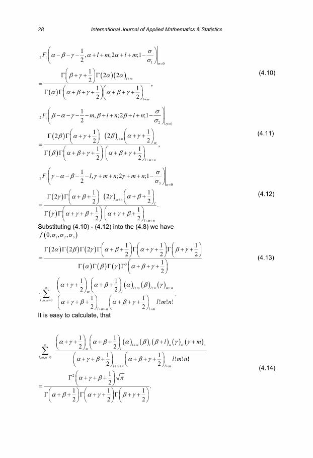
Using the formula analytical continuation for hypergeometric function of Gauss [18]


1, ; ; ,1 ;1 ;

1,1 ;1 ; ,

a

b

c b aF a b c y y F a c a b a

b c a y

c a by F b c b a b

a c b y

(4.4)

from expression (4.3) we get

2

2

2 1 2 1 2

2 2

2 2

1 1

2 2 2 2

, 0 2

2 2

2 2

1 1

2 2 2 2

, 0 2

, , , ; ; , ,

1,1 ;1 ;

! !

1,1 ;1 ;

! !

m pm m

m p m p

m pm m

m p m p

B x y z

y

x z F m pm p y

y

x z F m pm p y

(4.5)

Decomposing in a series hypergeometric function of Gauss, we receive

2

2

2 2

2 1 2 1 2

2 2

1 2 1 2

, , 0 2 2 2

2 2

2 2

1 2 1 2

, , 0 2 2 2

, , , ; ; , ,

11

! ! ! 1

11.

! ! ! 1

n

m pm n m n

m n p m p n

n

m pm n m n

m n p m p n

B x y z y

m px z

m n p y

y

m px z

m n p y

(4.6)

By virtue of identity

2 2 2

2 2 2

1 1 1 ,

1 1 1 ,

m p

n m p m n p

m p

n m p m n p

m p

m p

and changing the order of summation, from (4.6) we have

2

2

2 2

2 1 2 1 2

2 2

2 1 2 1

, , 0 2 2

2 2

2 2

2 1 2 1

, , 0 2 2

, , , ; ; , ,

1 1

1 ! ! !

1 1

1 ! ! !

m

n pm n p n m n

n m p m

m

n pm n p n m n

n m p m

B x y z y

x zn m p y

y

x zn m p y

(4.7)


By virtue of definition (4.2) of hypergeometric functions 3

2 1 2 3; , , ; ; , ,H a b b b c x y z , from

identity (4.7) we shall finally get the formula of an analytic continuation (4.1). Note, in paper [20] expansions of Lauricella’s hypergeometric functions from many variables were found.

5. THE STATEMENT OF THE CAUCHY PROBLEM

Consider the generalized Euler-Poisson-Darboux equation (1.1) in a characteristic triangle . The triangle is limited by straight lines 0 ,0 1 ; 1,0 ;

with tops in points 0,0O , 0,1A , 1,1B .

Definition. A regular solution of the equation (1.1) in the domain we call a

function ,u , which is continuous in the closed domain and has continuous derivatives

of the second order in the domain and satisfying the generalized Euler-Poisson-Darboux equation (1.1). Cauchy problem. Find a regular solution of the equation (1.1) in the domain , satisfying initial conditions

0lim , ,u 0 1 , (5.1)

2

0lim u u , 0 1 , (5.2)

where 2 2,C J C J C J C J are given functions, 0,1J is an

interval of an axis 0 . In the theory of degenerating equations of hyperbolic type, the main role is played the

function of Riemann 0 0, ; ,R , which for the equation (1.1) is defined as follows:

1. 0 0, ; ,R is a solution of the conjugate equation on variables ,

, 0.M R R R R R (5.3)

2. The function 0 0, ; ,R on characteristics 0 and 0 accordingly accept values

0 00 0 0

0 0 0 0

, ; ,R , (5.4)

0 00 0 0

0 0 0 0

, ; ,R , (5.5)

where 0 , 0 , .

3. The function 0 0, ; ,R is a solution of equation Volterra of the second kind


0

0 0 0

0 0 0 0

0 0 0 0

, ; , , ; ,

, ; , , ; , 1.

R R t dtt t

R t dt R t y dtdyt t

(5.6)

Let's construct the function of Riemann of generalized Euler-Poisson-Darboux equation.

6. THE FUNCTION OF RIEMANN GENERALIZED EULER-POISSON-DARBOUX EQUATION

The solution of the conjugate equation (5.3) we shall search in the form of

0 0 1 2 3, ; , , ,R P , (6.1)

where

0 0 0 0

P , (6.2)

0 0

1

0 0

, 0 0

2

0 0

, 3 0 0 . (6.3)

Calculating derivative of expression (6.1) and substituting in to the conjugate equation (5.3), we find

1 1 2 2 3 3 1 2 1 3 2 3

1 2 3

1 2 3 1 2 3

1 2 3 0,

A A A B B B

C C C D (6.4)

where

1 1 1 2 2 2 3 3 3, , ,A P A P A P

1 1 2 1 2 2 1 3 1 3 3 2 3 2 3, , ,B P B P B P

1 1 1 1 1 1 ,C P P P P P (6.5)

(6.5)

2 2 2 2 2 2 ,C P P P P P

3 3 3 3 3 3 ,C P P P P P

2 2

2 2.D P P P P

After elementary evaluations from (6.5) we get


1 1 121

PA , 2 2 22

11A P , 3 3A P ,

1 2 12 2

1 1B P , 3

2 1 2B P P , 3

3 2 2B P P ,

(6.6)

1 12

11 1 1C P , 2 22

1 1 1P

C , 3C P ,

2 2

1 1D P P P .

Substituting the received expressions (6.6) in to the equation (6.4), we define system of hypergeometric equation

1 1 1 2 1 3 1

2 2 1 2 2 3 2

3 3 1 3 2 3 3

1 1 2 3 1

2 2 1 3 2

3 1 2

1 1 1 1 1 0

1 1 1 1 1 0

0.

(6.7)

Considering a solution of the system of hypergeometric equations (3.7), we can find a solution of system (6.7)

1 2 3 2 1 2 3, , , ,1 ,1 ;1; , ,B . (6.8)

Substituting a solution (6.8) in to the representation (6.1), we define function of Riemann for the Cauchy problem

0 0 2 1 2 3

0 0 0 0

, ; , , ,1 ,1 ;1; , ,R B . (6.9)

Further, using function of Riemann (6.9), we shall solve the Cauchy problem for generalized Euler-Poisson-Darboux equation (1.1).

7. THE SOLUTION OF THE CAUCHY PROBLEM FOR GENERALIZED EULER-POISSON-DARBOUX EQUATION

We designate through the domain, limited by a segment 1 2PP of a straight line

( 0) and characteristics 1 0:PP , 2 0:PP . The following identity is true

, ,2

2 2 2 2.

RL u uM R

Ru uR uR Ru uR uR (7.1)


Integrating identity (7.1) on domain and applying Green's formula, we have

2 2 2 20,Ru uR uR d Ru uR uR d (7.2)

where 1 2 1 2PP PP PP is a boundary of domain ; taking 1 : 0PP d , 2 : 0PP d and

properties of the function of Riemann (6.9) into account , last identity we rewrite in the form of

0 0

0 0

0 0

2 1,

2 2

R Ru R u d u u R d . (7.3)

Calculate the first integral in a solution (7.3). Using the formula of the analytic continuation (4.1), from function of Riemann (6.9) we define

3

0 0 1 1 2 1 2 3

3

2 2 2 1 2 3

, ; , ; , ,1 ;2 ; , ,

1 ; ,1 ,1 ;2 2 ; , , ,

R PH

P H (7.4)

where2 1 2

0 0

1 2 1 1

0 0 0 0 0 0 0 0

1 22 2

0 0 0 0

1 2 3 0 0

0 0 0 0

, ,

1 2 2, ,

1 1 2

, , .

P P

(7.5)

Let's calculate derivatives of the function (7.4). Then we find

1 2

3 1

2 3

3 3 3

1 1 2 1 1 2 1 1 1 2 2

3 3 3

1 1 2 3 2 2 2 2 2 2 1

3 3

2 2 2 2 2 2 2 3

2 2 2

2 2 2 2 2

2 2 2 2 ,

R P H PH PH

PH P H P H

P H P H

(7.6)

1 2

3 1

2 3

3 3 3

1 1 2 1 1 2 1 1 1 2 2

3 3 3

1 1 2 3 2 2 2 2 2 2 1

3 3

2 2 2 2 2 2 2 3

2 2 2

2 2 2 2 2

2 2 2 2 ,

R P H PH PH

PH P H P H

P H P H

(7.7)

where3 3

2 2 1 2 3

3 3

2 2 1 2 3

2 ; , ,1 ;2 ; , , ,

2 2 1 ; ,1 ,1 ;2 2 ; , , .

H H

H H

Substituting found derivatives of the function of Riemann (7.6) - (7.7), in to the first integral of the solution (7.3) we get


2

2

R RR

3 3

1 2 1 1 2 2 2 2 2

1 12 2 2

2 2H P P P H P P

1 1

3 3

1 1 2 2 2 2 1 1 2 2 3 3

12 2 2

2PH P H (7.8)

3 3

1 1 2 2 2 2

2 22 2 2P H P H .

Considering the formula of derivation

3

2 1 2 3

1 2 3 3

2 1 2 3

; , , ; ; , ,

; , , ; ; , , ,

i j k

i j k

i j k j i j

i

H a b b b c x y zx y z

a b b bH a i j k b j b i b j c i x y z

c

(7.9)

and also by virtue of equalities

1 1 1

0 0

4P P P ,

2 2 2

0 0

2 1 1P P P ,

0 0 0 0 0 0

1 1 2 2

0 0 0 0

,

0 0 0 0

2 2 2 2

0 0 0 0

,

3 3 0 0 0 0 ,

from expression (7.8), follows

3

1 1 2

0 0

2 12

2 2

R RR PH

3

2 2 2

0 0

2 1 1 1 1 12 2

2 2P H (7.10)

1 1

3 3

1 1 2 2 2 2 1 1 2 2 3 3

12 2 2 .

2PH P H

Identity (7.10) we substitute in to the first integral of the solution (7.3) and we define

0

0

0

0

1 2

0 0

20

0 0

3

2 2 31 1

0 0

2lim 2 1

2

21 ; ,1 ,1 ;2 2 ;0, , .

v vv u d

H d

(7.11)


Taking

3

2 2 3 2 2 31 ; ,1 ,1 ;2 2 ;0, , ,1 ; ; , ,H (7.12)

into account, where confluent hypergeometric function of the Horn [16, 18]

2 2 3,1 ; ; , has a form

2

, 0

, ; ; , .! !

m nm m

m n m n

a ba b c x y x y

c m n (7.13)

Then the relation (7.11) will become

0

0

0

0

0

1 2

0 0

2 2 1 21 1

0 0 0 0

2lim

2

22 1 ,1 ; ; , ,

v vv u d

d

(7.14)

where

0 0

1 2 0 0

0 0

, .2

(7.15)

Further, we calculate the second integral in the formula (7.36). For this purpose in the expression (6.9), we shall select hypergeometric function on argument 2 .

0 0

2 1 3

, 00 0 0 0

, ; ,

1,1 ;1 ; .

1 ! !

m pm m

m p m p

R

F m pm p

(7.16)

We use the following formula [18]

, ; ; 1 , ; ;1

a zF a b c z z F a c b c

z, (7.17)

and from expression (7.16), we find

0 0 2

0 0 0 0

21 3

, 0 2

, ; , 1

1, ;1 ; .

1 ! ! 1

m pm m

m p m p

R

F m p m pm p

(7.18)

Considering equality

0 0 0 022 2

0 0 2 0 0

1 ,1

, (7.19)

we have


2

0 0

0 0 0 0

2 1 3

, 0

, ; ,

1, ;1 ; .

1 ! !

m pm m

m p m p

R

F m p m pm p

(7.20)

Now by the help of (7.21) we calculate expression under the second integral in the formula (7.3). Really, taking (7.20) into account, we define

0 00 0 0 0

2 1 3

, 0

lim lim

1, ;1 ; .

1 ! !

m pm m

m p m p

u u R

F m p m pm p

(7.21)

Using the following limits

0 0 0 0

1 10

0 0 0 0

lim2 2

, (7.22)

20

lim 1 , 3 3 0 00

lim ,

and also value of hypergeometric function of Gauss in a point 2 1 [18]

2

11 2, ;1 ;1

1 1

m p

m p

F m p m p ,

from (7.22), we define

0

2 1 22

0 0 0 0

lim

1 2 2,1 ;1 ; , ,

1

u u R

(7.23)

where 1 2, are defined by equality (7.15). Thus, the second integral in the formula (7.3) has

a form

0

0

0

0

0

2 1 22

0 0 0 0

1lim2

1 2 21,1 ;1 ; , .

2 1

u u R d

d

(7.24)

Substituting equalities (7.14) and (7.24) in to the formula (7.3), finally we find a solution of the Cauchy problem of generalized Euler-Poisson-Darboux equation


0

0

0

0

1 2

0 0

0 0 1 2 1 21 1

0 0 0 0

2 2 1 2

0 0 0 0

, ,1 ; ; ,

1,1 ;1 ; , ,

u k d

k d

(7.25)

where 1 2, are defined by equality (7.15) and

1 2

22k , 1

2 2

1 22

1k . (7.26)

It is not difficult to be convinced that, solutions of the Cauchy problem (7.26) satisfy to conditions of the Cauchy problem (5.1) - (5.2), and generalized Euler-Poisson-Darboux equation.

ACKNOWLEDGEMENT

I am grateful to Professor John Michael Rassias for his kind interest during the preparation of this paper.

REFERENCES

[1] G. Darboux. La Theorie Generale das Surfaces, Vol. 2, Gauthier-Villars, Paris, 1915.

[2] M. Saigo. A Certain boundary value problem for the Euler-Darboux equations, Math.

Japonica, 24 (1979), 377-385.

[3] M. Saigo. A Certain boundary value problem for the Euler-Darboux equations II, Math.

Japonica, 25 (1980), 211-220.

[4] M. Saigo. A Certain boundary value problem for the Euler-Darboux equations III, Math.

Japonica, 26 (1981), 103-119.

[5] A. Erdelyi, On the Euler-Poisson-Darboux equation. J. Analyse Math. 23 (1970), 89-102.

[6] W. Herbert, Riemann functions with several auxiliary variables. Forschunzentrum Graz,

Mathematisch-Statistische Sektion, Graz, 1981.

[7] D. W. Bresters, On the Euler-Poisson-Darboux equation. SIAM J. Math. Anal. 4 (1973), no. 1, 31-41,

[8] D. W. Bresters, On a generalized Euler-Poisson-Darboux equation. Ibid. 9 (1978), no. 5, 924-934.

[9] H. Wallner, The Riemann function of the differential equation ' 0zw z w .

Arch. Math. (Basel) 37 (1984), no. 5, 435-442.

[10] J. S. Lowndes, Cauchy problems for second-order hyperbolic differential equations with

constant coefficients. Proc. Edinburgh. Math. Soc. (2) 26 (1988), no. 3, 307-311.

[11] M. M. Smirnov, Equations of mixed type. Translations of Mathematical Monographs, 51,

American Mathematical Society, Providence, R. I., 1978, p. 232.

[12] J. M. Rassias, Mixed type Equations and Maximum Principles in fluid dynamics, 1983,


Symmetry Publ., Greece

[13] J. M. Rassias, Lecture Notes on Mixed Type Partial Differential Equations, World

Scientific, 144 p, 1990.

[14] J. M. Rassias, A maximum principle in 1nR . J. Math. Anal. Appl. 85 (1982), no. 1, 106-113.

[15] J. M. Rassias, An application of the theory of positive symmetric systems to a

degenerate multidimensional hyperbolic equation in 3R . Serdica 8 (1982), no. 3, 235-242

[16] P. Appell and J. Kampe de Feriet, Fonctions Hypergeometriques et Hyperspheriques;

Polynomes d'Hermite, Gauthier - Villars. Paris, 1926.

[17] A. Erdelyi, Integraldarstellungen fur Produkte Whittakerscher Funktionen. Nieuw Arch.

Wisk. 2, 20 (1939), 1-34.

[18] A. Erdelyi, W. Magnus, F. Oberhettinger and F. G. Tricomi, Higher Transcendental

Functions, vol. I, McGraw-Hill Book Company, New York, Toronto and London, 1953.

[19] P. O. Olsson, Analytic continuations of higher-order hypergeometric functions. J. Math.

Phys. 7 (1966), no 4, 702-710.

[20] A. Hasanov and H. M. Srivastava, Some decomposition formulas associated with the

Lauricella function r

AF and other multiple hypergeometric functions, Appl. Math. Lett.

19 (2006), no. 2, 113-121.


Uniqueness of the Solution of One Non-Local Boundary Value Problem for the Mixed Parabolic Type Equation

E. T. Karimov

Insitute of Mathematics, Uzbek Academy of Sciences F. Khodzhaev str. 29, Tashkent, 700125, Uzbekistan

E-mail: [email protected]

ABSTRACT

In the present work uniqueness of solution of boundary value problem with non-local conditions for mixed parabolic type equation is proven by the method of energy integrals. Moreover, using Fourier method eigenvalues and eigenfunctions of the considered problem are found.

Keywords and Phrases: Mixed Parabolic type equation; non-local boundary value problem;

eigenvalue and eigenfunction of problem.

Mathematics Subject Classification: 35M10; 35P05

1 INTRODUCTION

It is known that the theory of non-local problems is actual by itself as a

division of general theory of boundary-value problems for the partial differential

equations, and as a division of mathematics, which has numerous applications to the

mechanics, physics, biology and to other material sciences.

Note the work [1], where given main results on linear second order partial

differential equations of parabolic type and the works [2-5], where studied several

boundary problems for mixed type equations. In the book of J. M. Rassias [6] one

can find detailed explanations of methods using at solving boundary value problems

for mixed type equations. Especially, note works of A.L. Kerefov [7], E. T. Karimov

[8], A. S. Berdyshev and E. T. Karimov [9], and works of N. N. Shopolov [10] devoted

to studying non-local boundary value problems for mixed parabolic and mixed

parabolic-hyperbolic type equations, which results closely related to the present

work.


2 FORMULATION OF THE PROBLEM

We consider the equation

1

2

, 00

, 0

xx y

xx y

u u u x

u u u x (2.1)

in the domain 1 2D D D , in which 1 ( , ) : 1 0, 0 1D x y x y ,

2 ( , ) : 0 1, 0 1D x y x y , 1 2, are given complex numbers.

The Problem C. Find a function ( , )u x y , which satisfies the following conditions:

i) 2,1

, 1 2( , ) x yu x y C D C D D ; (2.2)

ii) 1 3 3( , )xu x y C D I I I ; (2.3)

iii) satisfies equation (2.1) in domain 1 2D D ;

iv) 1 2( 1, ) ( ), (1, ) ( ), 0 1u y y u y y y ; (2.4)

v) 1( ,0) ( ,1) ( ), 1 0,u x u x x x (2.5)

2( ,0) ( ,1) ( ), 0 1,u x u x x x (2.6)

where

1 ( , ) : 1,0 1 ,I x y x y 2 ( , ) : 0,0 1 ,I x y x y 3 ( , ) : 1,0 1I x y x y ,

( ), ( ) ( 1, 2)i iy x i are given real valued functions, moreover 1 2(0) (0),

1 1 1(0) (1) ( 1), 2 2 2(0) (1) (1) .

3 UNIQUENESS OF THE SOLUTION

Let the Problem C has two solutions 1u and 2u . We designate through

1 2U u u and obtain the following homogeneous problem C:

Homogeneous problem C. Find a solution of the equation

1

2

, 00

, 0,

xx y

xx y

U U U x

U U U x (3.1)

which satisfies conditions (2.2), (2.3), and the following conditions:

( 1, ) 0, (1, ) 0, 0 1U y U y y ; (3.2)

( ,0) ( ,1) 0, 1 0,U x U x x (3.3)

( ,0) ( ,1) 0, 0 1U x U x x . (3.4)


Theorem. If 1 2Re 0 is valid, then homogeneous problem C has trivial

solution.

Proof:

We prove this theorem by the method of energy integrals [6]. For this at 0x

we multiply equation (2.1) to ( , )U x y , which is complex-conjugate function of ( , )U x y :

1 0xx yU U U U ,

and integrate along the domain 1 ( , ) : 1 0, 0 1D x y x y :

1

2 2 2

1

1| | | | 0

2x x yx

D

U UU U U dxdy .

Using Green’s formula we have [6]

1

12 2

1

0

2 2

1

| | ( , ) ( , ) ( 1 , ) ( 1 , )

1| ( ,1 ) | | ( ,0) | 0.

2

x x x

D

U U dxdy U y U y U y U y dy

U x U x dx

(3.5)

Similarly at 0x we get the following equality:

2

12 2

2

1

2 2

| | (1 , ) (1 , ) ( , ) ( , )

1| ( ,1) | | ( , ) | 0,

2

x x x

D

U U dxdy U y U y U y U y dy

U x U x dx

(3.6)

in which 2 ( , ) : 0 1 , 1D x y x y .

We pass to the limit when 0 and separate the real parts of (3.5), (3.6).

After taking the following equality

Re ( 1, ) ( 1, ) Re ( 1, ) ( 1, )x xU y U y U y U y

and conditions (3.2) – (3.4) into account we obtain

12 2 2

1 2

0

Re | | | ( ,0) | 0.x

D

U U dxdy U x dx (3.7)

Further assume that 1 2Re 0 . Finally, taking condition (3.2) into account we

get ( , ) 0u x y in the domain D .

Theorem is proved.


It is easy to conclude that if homogeneous problem C has trivial solution, then

problem C has unique solution.

4 EIGENVALUES AND EIGENFUNCTIONS OF THE PROBLEM C

Definition. We call values of ( 1, 2)i i as an eigenvalues of the problem C, if at

these values of ( 1, 2)i i homogeneous problem C has non-trivial solution. These

non-trivial solutions we call as eigenfunctions of the problem C.

Corollary 1. The Problem C can have eigenvalues only outside of the domain

: Re 0 ( 1,2)i i i .

The solution of homogeneous problem C can be written as

( , ) ( ) ( )U x y X x Y y . (4.1)

Substituting (4.1) into the equation (3.1) at 0x and supposing ( ) 0, ( ) 0X x Y y ,

after some transformation we obtain

1 1

( ) ( )

( ) ( )

X x Y y

X x Y y, (4.2)

where 1 is any constant. From (4.2) we get

1 1

1

( ) ( ) 0

( ) ( ) 0.

X x X x

Y y Y y (4.3)

The condition (3.2) will pass to ( 1) 0, (0) 0X X . And condition (3.3) will have the

form of (0) ( 1)Y Y . After the solving the ordinary partial differential equations (4.3)

by the variation method at ( , ) 2

1 2 ( )m n n i m we get

2( ) sin , ( ) ( , /0)n iy

m nX x m x Y y e m n . (4.4)

Hence, non-trivial solution of homogeneous problem C in the domain 1D has the

form of

2( , ) ( ) ( ) sinn iy

mn m nu x y X x Y y e m x

Similarly we can find non-trivial solutions of homogeneous problem C

( , ) ( ) ( )mn m nu x y X x Y y at ( , ) 2

2 (1 2 ) ( )m n n i m in the domain 2D , in which

functions ( ), ( )m nX x Y y have the form of

(1 2 )( ) sin , ( ) ( , /0)n iy

m nX x m x Y y e m n .

One can see that ( 1,2)i i located outside of the domain ( see the Corollary 1).


Corollary 2. ( , ) 2

1 2 ( )m n n i m , ( , ) 2

2 (1 2 ) ( )m n n i m are eigenvalues, and

2( , ) sinn iy

mnu x y e m x , (1 2 )( , ) sinn iy

mnu x y e m x , ( , /0)m n are eigenfunctions

of the Problem C.

We note that existence of the solution of Problem C can be proven similarly to the

work [10].

REFERENCES

[1] A. M. Ilyin, A. S. Kalashnikov, and O. A. Oleynik (2002). Linear second order partial differential equations of the parabolic type. Journal of Mathematical Sciences, Vol. 108, No 4, pp. 435-542. The Russian version of this article is a reprint from the journal “Uspekhi Matematicheskikh Nauk” (1962, Vol. 17, issue 3(105), pp.3-146).

[2] M. H. Protter (1954). New boundary value problems for the wave equation and equations of mixed type. J. Rat. Mech. Anal., 3, 435-446.

[3] J. M. Rassias (1977). Mixed type partial differential equations. Ph. D. dissertation, U. C. Berkeley [Ph. D. thesis advisor: M. H. Protter].

[4] J. M. Rassias (1999). Existence of weak solutions for a parabolic elliptic- hyperbolic Tricomi problem. Tsukuba J. Math., 23, 37-54.

[5] J. M. Rassias (2002). Uniqueness of quasi-regular solutions for a bi-parabolic elliptic bi-hyperbolic Tricomi problem. Complex Variables, 47, pp.707 – 718.

[6] J. M. Rassias (1990). Lecture Notes on Mixed Type Partial Differential Equations. World Sci., Singapore.

[7] A. L. Kerefov (1979). Non-local boundary value problems for the parabolic type equations. Differensialnye uravnenija, Vol.15, No 1.

[8] E. T. Karimov (2005). About the Tricomi problem for the mixed parabolic-hyperbolic type equation with complex spectral parameter. Complex Variables: Theory and Application, Vol. 56, No 6, pp. 433 – 440.

[9] A. S. Berdyshev and E. T. Karimov (2006). Some non-local problems for the parabolic-hyperbolic type equation with non-characteristic line of changing type. Central European Journal of Mathematics, Vol. 4, No 2, pp. 183-193.

[10] N. N. Shopolov (1979). On one boundary value problem with non-local initial conditions for the mixed parabolic type equation I. Godishnik VUZ, Vol.15, No 2, pp.137-146.


Non-uniqueness of Transonic Flow past a Flattened Airfoil

Alexander G. Kuz’min1

1Institute of Mathematics and MechanicsSt Petersburg State University

28 University Ave., 198504 St Petersburg, [email protected]

ABSTRACT

A numerical analysis of inviscid and viscous transonic flows past a flattened airfoil is per-

formed. Non-unique solutions of boundary value problems for the Euler and Navier-Stokes

equations are obtained under certain conditions for flow parameters given on the far-field

boundary.

Keywords: transonic flow, airfoil, finite-volume solutions, stability, bifurcation.

2000 Mathematics Subject Classification: 76H05.

1 Introduction

Numerical studies of (Jameson, 1991), (Hafez and Guo, 1999a), (Hafez and Guo, 1999b) re-

vealed non-unique steady solutions of boundary value problems for the system of Euler equa-

tions governing inviscid flow. A detailed analysis of the non-uniqueness was performed by

(Ivanova and Kuz’min, 2004) and (Kuz’min, 2005) for flow past the airfoil

y(x) = ±0.06√

1 − (2x − 1)4 (1 − xm)2, 0 ≤ x ≤ 1. (1.1)

It was shown that transonic solutions are unique if m ≤ 8. At the same time, if 8.5 ≤ m ≤ 12and, consequently, airfoil’s curvature is small near the midchord x = 1/2, then there exist non-

unique solutions for certain ranges of the angle of attack α and Mach number M∞ given

on the far-field boundary.

In this paper, we analyze the non-uniqueness of transonic solutions for the airfoil ( with the

parameter m = 16:

y(x) = ±0.06√

1 − (2x − 1)4 (1 − x16)2, 0 ≤ x ≤ 1. (1.1′)

In particular, we demonstrate that at 0.825 < M∞ < 0.836, M∞ = 0.833, α = 0 there exist

both asymmetric and symmetric (with respect to the x−axis) steady solutions of the Euler

equations. The realization of a particular solution depends on the time history of M∞ and α.


2 Formulation of the problem and a numerical method

Let D be a domain of the plane (x, y) bounded by the airfoil (1.1′) and a C−type far-field

boundary Γ = Γ1∪Γ2∪Γ3∪Γ4, where Γ1 is the vertical segment x = 16, −15 ≤ y ≤ 15, while

the segments Γ2 and Γ3 are parallel to the freestream velocity vector, and Γ4 is a circular arc

(Fig. 1). The inviscid compressible adiabatic flow in the domain D is governed by the system

of Euler equations

∂ρ

∂t+

∂ρu

∂x+

∂ρv

∂y= 0,

∂ρu

∂t+

∂(ρu2 + p)∂x

+∂ρuv

∂y= 0,

∂ρv

∂t+

∂ρuv

∂x+

∂(ρv2 + p)∂y

= 0, (2.1)

∂e

∂t+

∂(e + p)u∂x

+∂(e + p)v

∂y= 0,

where p(x, y, t), ρ(x, y, t), u(x, y, t), v(x, y, t) are the static pressure, density, and compo-

nents of the velocity in x and y directions, respectively; e = p/(γ − 1) + ρ(u2 + v2)/2 is the

total energy per unit volume, γ = 1.4 is the ratio of specific heats.

A time-dependent solution [p, ρ, u, v] of the system ( admitting shock waves and contact dis-

continuities is to be found in the domain D under the initial-boundary conditions as follows.

The angle of attack α = acrtan(v∞/u∞) and the freestream Mach number M = M∞ < 1 are

given on the inflow part Γ4 of Γ, while the static pressure p = p∞ is given on the outflow part

Γ1. The normal velocity component vanishes on the airfoil and on Γ2 ∪ Γ3. The initial data are

either the uniform flow determined by the freestream conditions or a steady flow obtained pre-

viously for other values of M∞ and α. The Mach number is related to [p, ρ, u, v] by the formula

M2 = (u2 + v2)ρ/(γp).

To obtain numerical solutions of the above initial-boundary value problem, we used the NSCKE

finite-volume solver by (Mohammadi, 1994) in which the equations are discretized in space on

an unstructured mesh using the Roe scheme. The second-order accuracy is recovered by

means of a MUSCL reconstruction and Van Albada type limiters. The time integration was

performed by an explicit four-stage Runge-Kutta scheme. Steady solutions [p, ρ, u, v] of the

boundary value problem were calculated using relaxation in time and the local time-stepping

strategy,

p(x, y, t), ρ(x, y, t), u(x, y, t), v(x, y, t) → p(x, y), ρ(x, y), u(x, y), v(x, y) as t → ∞.

Computations were performed primarily on a nonuniform mesh of 733 × 215 grid points which

were clustered near the airfoil and in the vicinity of shock waves. Each of the two sides of

airfoil (1.1′) was represented by 265 nodes, whereas the outer boundary Γ of the domain

was discretized using 733 nodes. Test computations on a refined mesh yielded just marginal

corrections in the obtained flow field. The high accuracy of the method was confirmed by

application to transonic flow over the NACA 0012 airfoil at α = 1.25 deg and comparison with

results available in the literature (Delanyae, Geuzaine and Essers, 1997).


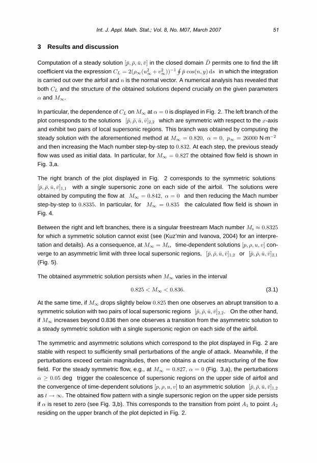
3 Results and discussion

Computation of a steady solution [p, ρ, u, v] in the closed domain D permits one to find the lift

coefficient via the expression CL = 2(ρ∞(u2∞ + v2∞))−1∮

p cos(n, y) ds in which the integration

is carried out over the airfoil and n is the normal vector. A numerical analysis has revealed that

both CL and the structure of the obtained solutions depend crucially on the given parameters

α and M∞.

In particular, the dependence of CL on M∞ at α = 0 is displayed in Fig. 2. The left branch of the

plot corresponds to the solutions [p, ρ, u, v]2,2 which are symmetric with respect to the x-axis

and exhibit two pairs of local supersonic regions. This branch was obtained by computing the

steady solution with the aforementioned method at M∞ = 0.820, α = 0, p∞ = 26000 N·m−2

and then increasing the Mach number step-by-step to 0.832. At each step, the previous steady

flow was used as initial data. In particular, for M∞ = 0.827 the obtained flow field is shown in

Fig. 3,a.

The right branch of the plot displayed in Fig. 2 corresponds to the symmetric solutions

[p, ρ, u, v]1,1 with a single supersonic zone on each side of the airfoil. The solutions were

obtained by computing the flow at M∞ = 0.842, α = 0 and then reducing the Mach number

step-by-step to 0.8335. In particular, for M∞ = 0.835 the calculated flow field is shown in

Fig. 4.

Between the right and left branches, there is a singular freestream Mach number Ms ≈ 0.8325for which a symmetric solution cannot exist (see (Kuz’min and Ivanova, 2004) for an interpre-

tation and details). As a consequence, at M∞ = Ms, time-dependent solutions [p, ρ, u, v] con-

verge to an asymmetric limit with three local supersonic regions, [p, ρ, u, v]1,2 or [p, ρ, u, v]2,1

(Fig. 5).

The obtained asymmetric solution persists when M∞ varies in the interval

0.825 < M∞ < 0.836. (3.1)

At the same time, if M∞ drops slightly below 0.825 then one observes an abrupt transition to a

symmetric solution with two pairs of local supersonic regions [p, ρ, u, v]2,2. On the other hand,

if M∞ increases beyond 0.836 then one observes a transition from the asymmetric solution to

a steady symmetric solution with a single supersonic region on each side of the airfoil.

The symmetric and asymmetric solutions which correspond to the plot displayed in Fig. 2 are

stable with respect to sufficiently small perturbations of the angle of attack. Meanwhile, if the

perturbations exceed certain magnitudes, then one obtains a crucial restructuring of the flow

field. For the steady symmetric flow, e.g., at M∞ = 0.827, α = 0 (Fig. 3,a), the perturbations

α ≥ 0.05 deg trigger the coalescence of supersonic regions on the upper side of airfoil and

the convergence of time-dependent solutions [p, ρ, u, v] to an asymmetric solution [p, ρ, u, v]1,2

as t → ∞. The obtained flow pattern with a single supersonic region on the upper side persists

if α is reset to zero (see Fig. 3,b). This corresponds to the transition from point A1 to point A2

residing on the upper branch of the plot depicted in Fig. 2.


Figure 6 demonstrates domains of the plane (M∞, α) in which the corresponding steady so-

lutions are stable and their structures are preserved (Fig. 6). The domains overlap revealing

a hysteresis with respect to variations of α and M∞. In the subdomains shown in light shade,

there exist two steady solutions, while in the subdomains shown in dark shade, there exist

three steady solutions of the boundary value problem formulated in Section 2. The realization

of a particular solution depends on the time history of the given boundary conditions.

The maximum of CL and the length of the non-uniqueness interval ( are greater in the case

under consideration as compared with that for airfoil ( with m = 10 and m = 12 studied by

(Ivanova and Kuz’min, 2004) and (Kuz’min, 2005). This is accounted for by the smaller cur-

vature of airfoil (1.1′) near x = 1/2 (see Fig. 7) and, consequently, a pronounced structural

instability of the transonic flow.

Non-unique solutions were also revealed for the system of Reynolds-averaged Navier-Stokes

equations which take into account the flow viscosity. In this case, the boundary condition on

the airfoil is the no-slip condition u = v = 0. To close the system of governing equations, we

used the Shear Stress Transport k − ω turbulence model (Menter, 1993). Numerical solutions

exhibited two, three, or four local supersonic regions as well as flow oscillations caused by the

boundary layer separation near airfoil’s trailing edge. Magnitudes of the oscillations of CL(t) at

Re = 5.4 × 106 are indicated by the shaded subdomains in Fig. 8. The singular Mach number

shifts from 0.833 to 0.836 in the case of viscous flow. Figure 9 demonstrates an instantaneous

pattern of the Mach number isolines in the viscous flow with three local supersonic regions at

M∞ = 0.832.

Acknowledgment

This work was supported by the Russian Foundation for Basic Research under grant 05-01-

00529.

References

Delanyae, M., Geuzaine, P. and Essers, J. (1997). Development and application of quadratic

reconstruction schemes for compressible flows on unstructured adaptive grids, AIAA Pa-

per, 97-2120: 250–260.

Hafez, M. and Guo, W. (1999a). Nonuniqueness of transonic flows, Acta Mechanica, 138: 177–

184.

Hafez, M. and Guo, W. (1999b). Some anomalies of numerical simulation of shock waves, part

1: inviscid flows, Computers and Fluids, 28: 701–719.

Ivanova, A. and Kuz’min, A. (2004). Nonuniqueness of the transonic flow past an airfoil, Fluid

dynamics (translated from Mekhanika Zhidkosti i Gaza), 39: 642–648.


Jameson, A. (1991). Airfoils admitting non–unique solutions of the euler equations, AIAA Pa-

per, 91-1625: 1–13.

Kuz’min, A. and Ivanova, A. (2004). The structural instability of transonic flow associated with

amalgamation/splitting of supersonic regions, J. of Theoretical and Computational Fluid

Dynamics, 18: 335–344.

Kuz’min, A. (2005). Bifurcation of transonic flow over a flattened airfoil, Frontiers of Fluid

Mechanics, World Scientific Publishing Company, Singapore, pp. 285–295.

Menter, F. (1993). Zonal two equation k − ω turbulence model predictions, AIAA Paper, 93-

2906: 1–13.

Mohammadi, B. (1994). Fluid dynamics computation with NSC2KE: an user-guide, release

1.0, Vol. RT-0164 of Techn. Report, INRIA, Le Chesnay.


Figure 1. A sketch of the domain D and the computational mesh.

Figure 2. Lift coefficient CL vs. M∞ at α = 0 for steady inviscid flow past airfoil (1.1′).


Figure 3. Mach number isolines for the steady inviscid flow at M∞ = 0.827, α = 0:(a) symmetric flow corresponding to point A1 in Fig. 2,(b) asymmetric flow corresponding to point A2 in Fig. 2.

Figure 4. Mach number isolines for the steady symmetric flow at M∞ = 0.835, α = 0.


Figure 5. Mach number isolines for the steady flow at M∞ = 0.833, α = 0:(a) asymmetric flow corresponding to point B2 in Fig.2,(b) asymmetric flow corresponding to point B1 in Fig.2.

Figure 6. Subdomains of the non-uniqueness in the plane of freestream parameters.


Figure 7. Upper parts of the airfoil (1.1) with m = 10, 12, 16, and the flattened airfoil byHafez and Guo (1999a).

Figure 8. Lift coefficient CL for airfoil (1.1′) at α = 0:1 - oscillating viscous flow, Re = 5.4 × 106, 2 - steady inviscid flow (reproduced from Fig.2).

Figure 9. Instantaneous Mach number isolines for the asymmetric viscous flow atM∞ = 0.832, α = 0, Re = 5.4 × 106.


Multiplier methods for mixed type equations

Kevin R. Payne

Dipartimento di Matematica “F. Enriques”Universita’ di Milano

Via Saldini, 5020133 Milano, [email protected]

ABSTRACT

We present a survey of recent results on existence, uniqueness and non-existence for

boundary value problems for equations of mixed elliptic-hyperbolic type. The common tech-

nical feature is the use of suitable integral identities and estimates that arise from well cho-

sen multipliers which are the infinitesimal generator of an invariance or almost invariance

of the differential equation.

Keywords: equations of mixed elliptic-hyperbolic type, multiplier methods, symmetry groups,

existence, nonexistence.

2000 Mathematics Subject Classification: 35M10, 35A05, 35B33, 35B45.

1 Introduction

The use of multiplier methods as an organized tool in the study partial differential equations

of mixed elliptic-hyperbolic type has its origins in the paper of Protter (1953), who, following

the suggestion of Friedrichs, generalized the uniqueness proof of Frankl’ (1945) for the Tricomi

problem by reinterpreting the proof in the language of suitable energy integrals. Since its in-

ception, this technique has become an indispensable tool due to its versatile technical power

as well as due to its global nature, which allows for an a posteriori understanding as to which

problems for mixed type equations are well posed. The problem of well-posedness is particu-

larly difficult in this setting with its mixture of qualitative types and the use of type-dependent

tools often results in a host of technical assumptions in order to glue together the pieces that

come from dividing the problem along its type change interface. The purpose of this note is

to give a survey of some recent developments in the use of multiplier methods for obtaining

results on existence, uniqueness and nonexistence for linear and nonlinear problems of mixed

type.

Before beginning our survey in earnest, we will briefly indicate what we mean by a multiplier

method and in which class of mixed type equations we will work. By a multiplier method, we

mean that given a partial differential equation

Lu = f in Ω ⊂ RN , (1.1)


where L is, for example, a second order linear differential operator with sufficiently smooth

coefficients in Ω and f a given function of x (and perhaps u or ∇u as well), one seeks to: 1)

multiply (1.1) by a suitable multiplier M [u]; 2) integrate over Ω; 3) manipulate the expression

using integration by parts and eventual boundary conditions to arrive at a potentially useful

integral identity. There is much artistry in both the choice of the multiplier M [u] as well as in

the choice of a suitable function space for u.

The class of mixed type equations we have in mind is that of Chaplygin type, in which the

differential operator has the form

L = K(y)∆xu + ∂2yu, (1.2)

where (x, y) ∈ Rn × R, ∆x is the Laplace operator on R

n with n ≥ 1 and the coefficient

K ∈ C0(R) satisfies

K(0) = 0 and K(y) = 0 for y = 0 (1.3)

so that the equation degenerates along the hypersurface y = 0. Our main interest concerns

cases in which K yields a change of type; that is, K also satisfies

yK(y) > 0 for y = 0, (1.4)

so that the equation (1.1) is of mixed type (elliptic for y > 0 and hyperbolic for y < 0), although

much of what will be discussed depends only on (1.2)-(1.3). The case n = 1 is particularly

important due to its longstanding connection with transonic fluid flow (cf. (Frankl’, 1945), (Bers,

1958), (Morawetz, 2004)) and also arises in problems of isometrically imbedding Riemannian

manifolds whose Gauss curvature changes sign (cf. (Lin, 1986)).

As a final preparation for our survey, we give a brief history of the use of multiplier methods in

mixed type equations. Protter’s original work, cited above, made use of a differential multiplier

M [u] = a(x, y)u + b(x, y)ux + c(x, y)uy in treating the question of uniqueness of quasi-regular

solutions to the Tricomi problem for an equation of Chaplygin type; that is,

Lu = K(y)uxx + uyy = f in Ω (1.5)

u|Γ = g, (1.6)

where Γ = σ ∪ AC ⊂ ∂Ω is particular proper subset of the boundary. More precisely, σ

is a piecewise regular curve in the elliptic region Ω+ (where y > 0), AC is a characteristic

of the operator L, and the type change function K obeys (1.3)-(1.4) and certain technical

conditions. Protter works directly on the second order equation and the function u essentially

lies in C2(Ω). Using a suitable choice of the unknown coefficients (a, b, c), integration by parts

together with the vanishing of u on σ ∪AC, yields an integral expression which is the sum of a

positive definite quadratic form on Ω and boundary integrals which are non-negative, provided

that the boundary satisfies a certain starlike condition, expressed by the non-negativity of a

certain differential one form. In this way, technical boundary geometry restrictions enter into

the hypotheses of the theorem. This result has been generalized to include other kinds of


boundary conditions of the form u = g on Γ ⊂ ∂Ω and to include additional classes of equations

in a host of papers too numerous to mention.

Soon afterward, Morawetz (1958), by exploiting duality along the lines used by Friedrichs

(1954) for hyperbolic equations, adapted the multiplier method in order to prove results on

existence for problems such as (1.5)-(1.6). In her approach, the differential equation (1.5) is

replaced by a more general first order system for (v1, v2) = (ux, uy) of the form

Lv =

[K∂x ∂y

∂y −∂x

] [v1

v2

]=

[f1

f2

].

The key step in her existence proof is a suitable a priori estimate for the formally skew-

symmetric operator L which comes from: 1) defining a multiplier matrix M in the form

M =

[b c

−Kc b

],

with M invertible almost everywhere; 2) taking a test function ϕ ∈ C1(Ω, R2) calibrated to

the adjoint boundary conditions, and 3) estimating (Lϕ,M−1ϕ) = (LMΦ, Φ) from above and

below, where

Φ = M−1ϕ or ϕ = MΦ.

A suitable multiplier pair (b, c) can be chosen to give the non-negativity of the form (LMΦ, Φ) if

the boundary is suitably starlike with respect to (b, c). Since L is formally skew-symmetric, one

recognizes this argument as a uniqueness result for the adjoint problem. At the same time, and

motivated in part by equations of mixed type, this technique was developed in a systematic way

by Friedrichs (1958) in his discovery of positive symmetric systems. These two papers are the

source of many important future developments, the former for attacks on problems related to

transonic flow such as (Morawetz, 1956), (Morawetz, 1957) and the latter for its prominence in

the theory of first order systems and as a touchstone in the development of type independent

tools for partial differential equations (cf. (Lax and Phillips, 1960), (Phillips and Sarason, 1966),

for example).

Shortly after the work of Morawetz, Berezanskii (1960), showed how one could use the multi-

plier technique directly on the second order equation to obtain a priori estimates on problems

such as (1.5)-(1.6), and its adjoint problem, by estimating from above and below the quadratic

forms (L∗u, M [u]) and (Lu,M [u]) with u ∈ C2(Ω), calibrated to the boundary condition, and M

a suitable differential multiplier. The form of the estimate for L∗ is

||u||H1Γ∗ ≤ C||L∗u||L2 , (1.7)

where H1Γ∗ is a Sobolev space of functions, calibrated to the adjoint boundary condition, which

are square integrable together with their first derivatives, perhaps with suitable weights. Such

an estimate on L∗ yields a uniqueness theorem for the adjoint problem as well as an exis-

tence theorem for the problem (1.5)-(1.6) and has been widely developed. With respect to the

approach of Morawetz, the existence results obtained directly by this method are weaker, the

solutions are guaranteed to lie only in L2, while the forcing term f can be more general (they

lie the dual space H−1Γ∗ ). On the other hand, if one wants to treat the second order equation,


this approach suggests the possibility of avoiding the passage to and return from the first order

system.

On the other hand, Didenko (1973) introduced an important variant in the multiplier technique

for problems such as (1.5)-(1.6), and its adjoint problem. His idea is to estimate from above

and below the quadratic forms (L∗u, M [u]) and (Lu,M [u]), where M [u] is now an integral

multiplier. For example, in order to estimate the adjoint L∗, one starts from u ∈ C20 (Ω), and

defines v = M [u] as the solution of the first order Cauchy problem

Mv := av + bvx + cvy = u in Ωv = 0 on Γ

where Γ is portion of the boundary carrying the boundary condition (1.6). Such a technique,

if it works, produces an a proiri estimate one step lower on the regularity scale with respect to

(1.7), namely

||u||L2 ≤ C||L∗u||H−1Γ

,

where H−1Γ is the dual space to H1

Γ equipped with its negative norm in the sense of Lax. This

approach retains the advantage of Berezanskii’s method by working directly on the second or-

der equation but it also produces solutions that are as strong as those obtained by Morawetz’s

technique.

There are two additional pieces of history which are important for what we have to say. First, in

a ground breaking paper (1970), Morawetz was able to use her method to obtain the first result

on well-posedness for weak solutions to the Dirichlet problem for mixed type equations. We

call such a boundary value problem closed in the sense that the boundary condition is placed

on the entire boundary, as opposed to an open boundary value problem in which the condition

is placed on a proper subset of the boundary. As the uniqueness theorems suggest, a closed

problem is typically over-determined in spaces of classical regularity. Such closed boundary

value problems are important for transonic flows about profiles, while the open problems are

linked to flows in nozzles (cf. (Bers, 1958), (Morawetz, 2004)). Morawetz’s result (1970) is valid

for the Tricomi equation (K(y) = y) and for domains which are lens-like and thin. Such re-

strictions are not particularly welcome in the applications to transonic flow since restrictions on

boundary geometry correspond to restrictions on airfoil shape and the approximation K(y) ∼ y

is valid only for nearly sonic speeds. Finally, we note that the method of multipliers has been

used to prove uniqueness theorems for semilinear boundary value problems of mixed type, as

done by Gvazava (1970), Rassias (1986) and others.

The recent progress we which to describe can be summarized in the following way. First,

we identify a class of multipliers naturally associated to the differential operators of the form

(1.2)-(1.4); namely, those which are the infinitesimal generators of the symmetry group for the

differential operator. This group has been calculated in (Lupo and Payne, 2005) and will be

discussed in section 2. Second, we apply variants of the methods of Berezanskii and Didenko

to the Dirichlet problem in order to find robust results on the existence and uniqueness of weak

solutions for such closed boundary value problems, which generalize the particular result of

Morawetz (1970). These results have been proven in (Lupo, Morawetz and Payne, in press)


and will be discussed in section 3. Finally, we give results on the nonexistence of nontrivial

solutions for semilinear equations of mixed type with various boundary conditions. These are

results from (Lupo and Payne, 2003) and (Lupo, Payne and Popivanov, 2006) and will be

discussed in section 4. The key ingredient is our systematic use of multipliers which generate

an invariance or almost invariance in the differential operator.

2 Symmetry groups and multiplier classes

In the art of choosing a useful multiplier for a given partial differential equation, it is a good idea

to think of the complete symmetry group associated to the differential operator (or its principal

part). The reason for this is fairly simple. If one has a continuous one parameter symmetry

group of variational or divergence type associated to a differential equation

Lu = 0, (2.1)

then Noether’s theorem ensures the existence of a conservation law associated to the solutions

of the differential equation; that is, an equation of the form

div U = 0,

which must be satisfied by every sufficiently regular solution of (2.1), where U is a nonlinear

function of (x, y, u,∇u). Integration of the conservation law over a domain then yields the

vanishing of a certain boundary integral. The same integral identity results if one uses the mul-

tiplier method with M [u] chosen as the infinitesimal generator of the one parameter symmetry

group applied to u. Hence, in some sense, the simplest possible integral identities are those

that result from an invariance property of the differential operator, or of its principal part.

We now recall briefly the results in (Lupo and Payne, 2005) on the symmetry groups for the

equation (2.1) with L of the form (1.2)-(1.4). The largest possible symmetry group results from

the particular choice of power type degeneration

K(y) = y|y|m−1, m > 0

(or K(y) = ±|y|m). The equation (2.1) is the Euler-Lagrange equation for the Lagrangian

L(y,∇u) =12

(K(y)|∇xu|2 + u2

y

). (2.2)

One has, apart from certain trivial symmetries for these linear and homogeneous equations,

symmetries coming from: 1) translations in the “space variables” x; 2) rotations in the space

variables; 3) certain anisotropic dilations; 4) inversion with respect to a well chosen hypersur-

face (cf. Theorem 2.5 of (Lupo and Payne, 2005)).

More precisely, the trivial one parameter symmetry groups arise from the fact that if u solves

(2.1) then so does u+ εβ with β any solution of (2.1) and ε ∈ R. The non trivial symmetries are

represented by the fact that if u solves (2.1) with K(y) = y|y|m−1,m > 0, then so do

uk;ε(x, y) = Tk;εu(x, y) = u(x − εek, y) (2.3)


uj,k;ε(x, y) = Rj,k;εu(x, y) = u(Aj,k;εx, y) (2.4)

uλ(x, y) = Sλu(x, y) = λ−p(m,N)u(λ−(m+2)x, λ−2y

)(2.5)

and

uk;ε(x, y) = Ik;εu(x, y) = D−q(N,m)k,ε u

⎛⎝x + εdek

Dk,ε,

y

D2/(m+2)k,ε

⎞⎠, (2.6)

where ε ∈ R (and |ε| is small in (2.6)), λ > 0, ekNk=1 is the standard basis of R

N , Aj,k;ε is the

ε-rotation in the xj − xk plane,

p(m,N) =N(m + 2) − 2

2> 0,

Dk,ε(x, y) = 1 + 2εxk + ε2d(x, y),

where

d(x, y) = |x|2 +4

(m + 2)2y|y|m+1, (2.7)

and

q(m,N) =N(m + 2) − 2

2(m + 2)> 0.

The same result holds for the degenerate elliptic/hyperbolic cases where K(y) = ±|y|m where

it is enough to replace y|y|m+1 with ±|y|m+2 in (2.7). The symmetries (2.3)-(2.5) are variational

in the sense that they leave invariant the integral of the Lagrangian (2.2) while the symmetry

(2.6) is a divergence symmetry and is only locally well defined. All yield associated conserva-

tion laws.

The infinitesimal generators of the nontrivial symmetries are given by the vector fields

vTk =

∂

∂xk, k = 1, . . . , N (2.8)

vD = (m + 2)x · ∇x + 2y∂

∂y− N(m + 2) − 2

2u

∂

∂u, (2.9)

vRjk = xk

∂

∂xj− xj

∂

∂xk, 1 ≤ j < k ≤ N (2.10)

vIk = −d(x, y)

∂

∂xk+ 2xkx · ∇x +

4m + 2

xky∂

∂y

−N(m + 2) − 2m + 2

xku∂

∂u, k = 1, . . . , N (2.11)

and together with the trivial symmetries generate the complete symmetry group (cf. Theorem

2.5 of (Lupo and Payne, 2005)). The proof of this claim exploits well known infinitesimal tech-

niques for classifying the infinitesimal generators

v =N∑

i=1

ξi(x, y, u)∂

∂xi+ η(x, y, u)

∂

∂y+ ϕ(x, y, u)

∂

∂u


of symmetries, where v is thought of as a vector field which acts an open subset M of the 0-jet

space, RN+1×U (0) R

N+1×R (the space of values for independent and dependent variables)

together with the action of their prolongations onto higher order jet spaces (which includes the

values of higher order derivatives of u). See the Appendix of (Lupo and Payne, 2005) for

details. See also (Payne, in press) for the relation between the symmetry group and the class

of conformal transformations with respect to a certain singular Riemannian metric associated

to the operator L

Hence, we obtain a class of potentially useful differential multipliers of the form M [u] = v(u)with v one of the vector fields in (2.8)-(2.11) or a linear combination of them.

3 Well posedness for the Dirichlet problem

In this section, we examine the question of well-posedness for the Dirichlet problem for a

second order linear partial differential equation of mixed elliptic-hyperbolic type. That is, given

f ∈ H0, we ask if it is possible to show the existence of a unique u ∈ H1 which solves in some

reasonable sense the problem

Lu = K(y)uxx + uyy = f in Ω (3.1)

u = 0 on ∂Ω (3.2)

where H0,H1 are functions spaces to be determined, K ∈ C1(R2) satisfies

K(0) = 0 and yK(y) > 0 for y = 0, (3.3)

Ω is a bounded open and connected subset of R2 with piecewise C1 boundary. We will assume

throughout that

Ω± := Ω ∩ R2± = ∅, (3.4)

so that (3.1) is of mixed elliptic-hyperbolic type. We will call Ω a mixed domain if (3.4) holds.

As noted in the introduction, while the Dirichlet problem (3.1)-(3.2) is classically well-posed for

an elliptic operator L, the presence of a hyperbolic subregion Ω− leads to an over-determined

problem in spaces of classical regularity. This phenomenon is well known for purely hyper-

bolic equations, as first noted by Picone (1910). From a suitable uniqueness theorem, one

can show that if u is a sufficiently smooth solution to (1.1) which vanishes only on a proper

subset of the boundary Γ = ∂Ω \ Σ, it must vanish on Ω. Hence, if one wants to impose the

boundary condition on all of the boundary, one must expect in general that some real singu-

larity must be present. Moreover, in order to prove well-posedness, one must make a good

guess about where to look for the solution; that is, one must choose some reasonable function

space which admits a singularity strong enough to allow for existence but not so strong as to

lose uniqueness. This, in practice, has proven to be the main difficulty of the problem.

In order to present the well-posedness results for (3.1)-(3.2), we would like to first make precise

the setting in which we will work. The function K ∈ C1(R) will be taken to satisfy (3.3) and


additional assumptions as necessary. In all that follows, Ω will be a bounded mixed domain

(open, connected, satisfying (3.4)) in R2 with piecewise C1 boundary so that we may apply the

divergence theorem and ν will denote the external normal field. Since the differential operator

(3.1) is invariant with respect to translations in x, we may assume that the origin is the point on

the parabolic line AB := (x, y) ∈ Ω : y = 0 with maximal x coordinate; that is, B = (0, 0). This

will simplify certain formulas without reducing the generality of the results. We will sometimes

require that Ω is star-shaped with respect to the flow of a given (Lipschitz) continuous vector

field V = (V1(x, y), V2(x, y)); that is, for every (x0, y0) ∈ Ω one has Ft(x0, y0) ∈ Ω for each

t ∈ [0, +∞] where Ft(x0, y0) represents the time-t flow of (x0, y0) in the direction of V .

We will make use of several natural spaces of functions and distributions. We define H10 (Ω; K)

as the closure of C∞0 (Ω) (smooth functions with compact support) with respect to the weighted

Sobolev norm

||u||H1(Ω;K) :=[∫

Ω

(|K|u2x + u2

y + u2)

dxdy

]1/2

.

Since u ∈ H10 (Ω; K) vanishes weakly on the entire boundary, one has a Poincare inequality:

there exists CP = CP (Ω,K)

||u||2L2(Ω) ≤ CP

∫Ω

(|K|u2x + u2

y

)dxdy, u ∈ H1

0 (Ω; K). (3.5)

The inequality (3.5) is proven in the standard way by integrating along segments parallel to the

coordinate axes for u ∈ C10 (Ω) and then using continuity. An equivalent norm on H1

0 (Ω; K) is

thus given by

||u||H10 (Ω;K) :=

[∫Ω

(|K|u2x + u2

y

)dxdy

]1/2

. (3.6)

We denote by H−1(Ω; K) the dual space to H10 (Ω; K) equipped with its negative norm in the

sense of Lax

||w||H−1(Ω;K) := sup0 =ϕ∈C∞

0 (Ω)

|〈w,ϕ〉|||ϕ||H1

0 (Ω;K)

, (3.7)

where 〈·, ·〉 is the duality bracket and one has the generalized Schwartz inequality

|〈w,ϕ〉| ≤ ||w||H−1(Ω;K)||ϕ||H10 (Ω;K), w ∈ H−1(Ω; K), ϕ ∈ H1

0 (Ω; K). (3.8)

One clearly has a rigged triple of Hilbert spaces

H10 (Ω; K) ⊂ L2(Ω) ⊂ H−1(Ω; K),

where the scalar product (on L2 for example) will be denoted by (·, ·)L2(Ω).

It is routine to check that the second order operator L in (3.1) is formally self-adjoint when

acting on distributions D′(Ω) and gives rise to a unique continuous and self-adjoint extension

L : H10 (Ω; K) → H−1(Ω; K) (3.9)


We will also make use of suitably weighted versions of L2(Ω) and their properties. In particular,

for K ∈ C1(R) satisfying (3.3) we define

L2(Ω; |K|−1) := f ∈ L2(Ω) : |K|−1/2f ∈ L2(Ω),

equipped with its natural norm

||f ||L2(Ω;|K|−1) =[∫

Ω|K|−1f2 dxdy

]1/2

,

which is the dual space to the weighted space L2(Ω; |K|) defined as the equivalence classes

of square integrable functions with respect to the measure |K| dxdy; that is, with finite norm

||f ||L2(Ω;|K|) =[∫

Ω|K|f2 dxdy

]1/2

.

One has the obvious chain of inclusions

L2(Ω; |K|−1) ⊂ L2(Ω) ⊂ L2(Ω; |K|),

where the inclusion maps are continuous and injective (since K vanishes only on the parabolic

line, which has zero measure).

As a first step, using standard functional analytic techniques, one can obtain results on distri-

butional existence and strong uniqueness for solutions to the Dirichlet problem (3.1)-(3.2). The

key point is to obtain a suitable a priori estimate by adapting the multiplier method of Berezan-

skii to this closed boundary value problem and selecting the test function to have compact

support. One obtains the following result

Theorem 3.1. Let Ω be any bounded region in R2 with piecewise C1 boundary. Let K ∈ C1(R)

be a type change function satisfying (3.3) and

K ′ > 0 (3.10)

∃δ > 0 : 1 +(

2K

K ′

)′≥ δ (3.11)

a) There exists a constant C1(Ω,K) such that

||u||H10 (Ω;K) ≤ C1||Lu||L2(Ω), u ∈ C2

0 (Ω). (3.12)

b) For each f ∈ H−1(Ω; K) there exists u ∈ L2(Ω) which distributionally solves (3.1)-(3.2) in

the sense that

(u, Lϕ)L2 = 〈f, ϕ〉, ϕ ∈ H10 (Ω; K) : Lϕ ∈ L2(Ω). (3.13)

This theorem is the union of Lemma 2.1 and Theorem 2.2 of (Lupo et al., in press), where the

complete proof is given. It should be noted that, since L is formally self-adjoint, the estimate

(3.12) also holds for Lt = L and that, in (3.13), L is the self-adjoint extension (3.9). The

estimate (3.12) follows from the multiplier method in which one considers an arbitrary u ∈


C20 (Ω) and seeks to estimate the expression (Mu,Lu)L2 from above and below where Mu =

au + bux + cuy is the multiplier to be determined. Using

a ≡ −1, b ≡ 0, c = c(y) = max0,−4K/K ′ (3.14)

one has the needed positive lower bound, while the Cauchy-Schwartz inequality is used for the

upper bound. The two estimates are combined with the Poincare inequality (3.5) to complete

the estimate (3.12). The proof of the existence in part b is a standard argument using the

Hahn-Banach theorem and the Riesz representation theorem.

The estimate (3.12) also shows that sufficiently strong solutions must be unique. We say

that u ∈ H10 (Ω; K) is a strong solution of the Dirichlet problem (3.1)-(3.2) if there exists an

approximating sequence un ∈ C20 (Ω) such that

||un − u||H1(Ω;K) → 0 and ||Lun − f ||L2(Ω) → 0 as n → +∞

The following theorem is an immediate consequence of the definition.

Theorem 3.2. Let Ω be any bounded region in R2 with piecewise C1 boundary. Let K ∈ C1(R)

be a type change function satisfying (3.3), (3.10) and (3.11). Then any strong solution of the

Dirichlet problem (3.1)-(3.2) must be unique.

Remarks:

1. The class of admissible K is very large and includes the standard models for transonic

flow problems such as the Tricomi equation with K(y) = y and the Tomatika-Tamada equation

K(y) = A(1 − e−2By) with A,B > 0 constants.

2. The result also holds for non strictly monotone functions such as the Gellerstedt equation

with K(y) = y|y|m−1 where m > 0. In this case, one can check that in place of (3.14) it is

enough to choose the dilation multiplier, introduced in (Lupo and Payne, 2003), whose principal

part was given in (2.9)

a ≡ 0, b = (m + 2)x, c = 2y.

3. No boundary geometry hypotheses have yet been made; in particular, there are no star-like

hypotheses on the elliptic part and no sub-characteristic hypotheses on the hyperbolic part.

These kinds of hypotheses will enter when we look for solutions in a stronger sense.

It is clear that the distributional existence is in a very weak sense; too weak, in fact, to be

very useful. In particular, the sense in which the solution vanishes at the boundary is only by

duality and one may not have uniqueness. Example 2.4 of (Lupo et al., in press) gives one

way in which things may go wrong. In any case, the existence result is a first general indication

that while the closed Dirichlet problem is generically over-determined for regular solutions, it is

generically not over-determined if one looks for a solution which is taken in a sufficiently weak

sense. Moreover, while uniqueness generically holds for strong solutions, one must show that

such strong solutions exist.

We are now ready for the well-posedness result, which shows that there is a way to steer a

course between the weak existence and the strong uniqueness result for the Dirichlet problem


by following the path laid out by Didenko (1973) for open boundary value problems. The suit-

able notion of solutions (called generalized solutions by Didenko in the case of open boundary

conditions) is contained in the following definition.

Definition 3.3. We say that u ∈ H10 (Ω; K) is a weak solution of the Dirichlet problem (3.1)-(3.2)

if there exists a sequence un ∈ C∞0 (Ω) such that

||un − u||H10 (Ω;K) → 0 and ||Lun − f ||H−1(Ω;K) → 0, for n → +∞

or equivalently

〈Lu, ϕ〉 = −∫

Ω(Kuxϕx + uyϕy) dxdy = 〈f, ϕ〉, ϕ ∈ H1

0 (Ω,K),

where 〈·, ·〉 is the duality pairing between H10 (Ω; K) and H−1(Ω; K), L is the continuous exten-

sion defined in (3.9), and the relevant norms are defined in (3.6) and (3.7).

Our first result concerns the Gellerstedt operator; that is, with K of pure power type

K(y) = y|y|m−1, m > 0. (3.15)

Theorem 3.4. Let Ω be a bounded mixed domain with piecewise C1 boundary and parabolic

segment AB with B = 0. Let K be of pure power form (3.15). Assume that Ω is star-shaped

with respect to the vector field V = (−(m + 2)x,−µy) where µ = 2 for y > 0 and µ = 1 for

y < 0. Then

a) there exists C1 > 0 such that

||u||L2(Ω;|K|) ≤ C1||Lu||H−1(Ω;K), u ∈ C∞0 (Ω). (3.16)

b) for each f ∈ L2(Ω; |K|−1) there exists a unique weak solution u ∈ H10 (Ω; K) in the sense of

Definition 3.3 to the Dirichlet problem (3.1)-(3.2).

Note that the theorem allows for both non lens-like and lens-like domains and hence relaxes

substantially the restrictions on the geometry of the boundary with respect to the original re-

sult of Morawetz (1970). Moreover, the star-shaped assumption implies that the hyperbolic

boundary is non-characteristic.

This theorem is the union of Lemma 3.3 and Theorem 3.2 of (Lupo et al., in press). The ex-

istence in part b) follows from the a priori estimate of in much the same way as in Theorem

2.1. The uniqueness follows also from the estimate and the Definition 2.3. To obtain the esti-

mate (3.16), the basic idea is to adapt the Didenko multiplier method to this closed boundary

value problem; that is, to estimate from above and below the expression (Iu, Lu)L2(Ω) for each

u ∈ C∞0 (Ω) where v = Iu is the solution to the following auxiliary Cauchy problem

Mv := av + bvx + cvy = u in Ωv = 0 on ∂Ω \ B

where B = (0, 0) is the righthand endpoint of the parabolic line and

a ≡ −1/4, (b, c) = −V = ((m + 2)x, µy). (3.17)


This multiplier is almost the principal part the dilation and translation multipliers (2.9); it has

been fudged a bit in the hyperbolic region in order to obtain the necessary positivity in a key

step of the proof. One analyzes first the properties of the solution v, which is shown to lie in

C∞(Ω±)∩C0(Ω)∩H10 (Ω; K). Then one estimates from below where the choice (3.17) ensures

the positivity of the quadratic form (Iu, Lu). The rest of the estimate proceeds as before, using

the generalized Schwartz inequality (3.8), continuity properties of the differential operator M ,

and the Poincare inequality (3.5).

Remarks:

1. One can eliminate almost entirely the boundary geometry restrictions in the elliptic part of

the domain by patching together the a priori estimate (3.16) with an easy estimate on elliptic

subdomains using the multiplier Mu = u (see Theorem 3.4 of (Lupo et al., in press)).

2. One can replace the type change functions K of pure power type with more general forms

in which there is a bound on the variation of (K/K ′)′ for y small (see Proposition 3.5 of (Lupo

et al., in press)).

3. Moreover, it should be possible to relax the regularity assumptions on the type change

function K. For example, this should be the case for the Lavrentiev-Bitsadze equation in which

K(y) = sign(y) (Lavrentiev and Bitsadze, 1950). This equation has been well studied for

problems with open boundary conditions; for example, see (Rassias, 1990) for techniques

along the lines of Protter and Berezanskii.

4. With respect to the original result of Morawetz, our improvements are due in part from the

fact that we work directly on the second order equation instead of reducing to a first order

system. Working with the equation allows for a greater freedom in choosing the multipliers

(a, b, c); for the first order system there is no coefficient corresponding to a.

5. The norm H1(Ω; K) employed here has a weight |K| which vanishes on the entire parabolic

line and hence one might worry that the solution is not locally H1 due to the term |K|u2x. In fact,

the solution does lie in H1loc(Ω) as is shown in section 5 of (Lupo et al., in press), which contains

the beginnings of a regularity theory. On the other hand, the norms used in (Morawetz, 1970)

for treating the equation by way of a first order system were carefully constructed so as not to

have weights vanishing on the interior.

6. In (Lupo et al., in press), we have also established well-posedness for closed problems

with mixed boundary conditions; Dirichlet conditions on the elliptic boundary and conormal

conditions on the hyperbolic boundary. The conormal condition is natural for transonic flow

problems when the unknown is a perturbation of the velocity potential. On the other hand, for

the Lavrentiev-Bitsadze operator, Pilant (1985), has obtained a result similar in spirit to that of

Morawetz (1970) for the full conormal problem. His result follows the idea of Morawetz and

has similarly strong restrictions on the geometry of the boundary, which must be lens-like and

thin. Attempts to handle general classes of equations in general domains for the full conormal

problem are in progress.


4 Nonexistence for semilinear problems

It is well known, starting from the seminal paper of Pohozaev (1965), that the homogeneous

Dirichlet problem for semilinear elliptic equations such as ∆u + u|u|p−2 = 0 in Ω a bounded

subset of Rn, with n ≥ 3, will permit only the trivial solution u ≡ 0 if the domain is star-shaped,

the solution is sufficiently regular, and p > 2∗(n) = (n + 2)/(n − 2) the critical exponent in

the Sobolev embedding of H10 (Ω) into Lp(Ω) for p ≤ 2∗(n) which fails to be compact at the

critical exponent. The proof of this result hinges upon a multiplier method in which one uses

the infinitesimal generator of the invariance of the Laplace operator with respect to dilations.

Hence, there arises the natural question of whether an analogous result holds for equations of

mixed type. That is, if L is a mixed type operator of Gellerstedt type

L = K(y)∆xu + ∂2yu, K(y) = y|y|m−1 with m > 0, (4.1)

one would like to know if sufficiently smooth solutions to the problem

Lu + F ′(u) = 0 in Ω (4.2)

u = 0 on Σ ⊆ ∂Ω (4.3)

must vanish identically in Ω if F a nonlinearity with a suitable notion of supercritical growth.

The answer is yes, as has been shown in (Lupo and Payne, 2003) and (Lupo et al., 2006).

The proof for the closed Dirichlet problem (Σ = ∂Ω) is almost completely analogous with the

classical elliptic case, while for open boundary value problems, there is a critical difference in

that one must be able to control the sign of additional boundary integrals. In many cases, we

are able to control these terms by using a suitable Hardy-Sobolev inequality.

In order to state the main results, we need to recall a few notions. Here Ω ⊂ RN+1 will again

be bounded with a piecewise C1 boundary. The hyperbolic boundary Σ− = ∂Ω ∩ RN+1− will be

called sub-characteristic for L if one has

K(y)|νx|2 + ν2y ≥ 0, on Σ− (4.4)

where ν = (νx, νy) is the (external) normal field on the boundary. This normal field is well

defined with the possible exception of a finite number of points which will create no essential

difficulty. If the inequality (4.4) holds in the strict sense, we will call Σ− strictly sub-characteristic

which just means that Σ− is a piece of a spacelike hypersurface for the operator L which is

hyperbolic for y < 0. The operator L in (4.1) is invariant with respect to the anisotropic dilation

whose infinitesimal generator is

V = −N∑

j=1

(m + 2)xj∂xj − 2y∂y (4.5)

(cf. (2.14)). This Lipschitz continuous vector field V defines the class of domains which are

admissible for the nonexistence principle; namely, those that are V -star-shaped, as defined in


section 3. Furthermore, we recall that if Ω is V -star-shaped then ∂Ω will be V -star-like in the

sense that on ∂Ω one has

(α, β) · ν ≥ 0 (4.6)

where α = (α1, . . . , αN ) and ν is the external unit normal to ∂Ω (cf. Lemma 2.2 of (Lupo and

Payne, 2003)). If the inequality (4.6) holds in the strict sense, we will say that ∂Ω is strictly

V -star-like. The differential operator L is also invariant with respect to translations in the x

variables, so one may normalize a given problem by assuming a particular location of the

origin without loss of generality, as done in section 3.

The dilation generated by V in (4.5) also gives rise to a critical exponent

2∗(N,m) =2[N(m + 2) + 2]N(m + 2) − 2

(4.7)

for the embedding of the weighted Sobolev space H10 (Ω; m) into Lp(Ω) where

||u||2H10 (Ω;m) :=

∫Ω

(|y|m|∇xu|2 + u2y

)dxdy

defines a natural norm for which to begin the search for weak solutions (cf. Proposition 2.4

of (Lupo and Payne, 2003) and section 3 of (Lupo and Payne, 2005)). More precisely, this

norm is the natural norm for variational solutions where one notes that the equation (4.2) is

the Euler-Lagrange equation associated to the functional J(u) =∫Ω (L(y,∇u) + F (u)) dxdy

where L(y,∇u) is the Lagrangian defined in (2.4). One has the following result (cf. Theorem

2.1 of (Lupo et al., 2006)).

Theorem 4.1. Let Ω be mixed type domain which is star-shaped with respect to the generator V

of the dilation invariance defined in (4.5) and whose hyperbolic boundary is sub-characteristic

in the sense (4.4). Let u ∈ C2(Ω) be a solution to (4.1)-(4.3) with F ′(u) = u|u|p−2. If p >

2∗(N,m) the critical Sobolev exponent (4.7), then u ≡ 0. If, in addition, ∂Ω is strictly V -star-like

and Σ− is strictly sub-characteristic, then the result holds also for p = 2∗(N,m).

We recall only the outline of the proof. Consider the primitive F satisfying F (0) = 0. One

multiplies (4.2) by Mu = −V u and integrates by parts and uses the boundary condition u =F (u) = 0 on ∂Ω to find the Pohozaev type identity calibrated to the dilation invariance

∫Ω

[(N(m + 2) + 2)F (u) − (N(m + 2) − 2)

2uF ′(u)

]dxdy =

∫∂Ω

W · ν dσ (4.8)

where

W = [(m + 2)x · ∇xu + 2yuy](K∇xu, uy) − L((m + 2)x, 2y)

and L is the Lagrangian defined in (2.2). In the supercritical case p > 2∗(N,m), if u is nontrivial,

then one arrives at a contradiction as the left hand side of (4.8) is negative, while the right

hand side is non-negative if u vanishes on the boundary which is assumed starlike and sub-

characteristic. In the critical case p = 2∗(N,m), if the boundary is strictly starlike, then the

identity (4.8) shows that the normal derivative of u vanishes on the boundary (together with u).

Another multiplier identity using M [u] = uy then shows that u vanishes on Ω.


We now turn our attention to the more difficult case in which the boundary condition is placed

on a proper subset Σ of the boundary ∂Ω. As a rule of thumb, Σ will be chosen in order to

yield a uniqueness theorem for the linear version of the problem. After all, the nonexistence

of nontrivial solutions for the semilinear problem can be viewed as a uniqueness theorem. For

simplicity, we will describe the simplest case, namely the Tricomi problem in dimension two,

but we will make some remarks about generalizations at the end of the section. We consider

the problem

K(y)uxx + uyy + F ′(u) = 0 in Ω (4.9)

u = 0 on Σ = σ ∪ AC, (4.10)

where K(y) = y|y|m−1 with m > 0, σ is an arc in the elliptic region and AC,BC are character-

istics of negative, positive slope for L = K(y)∂2x + ∂2

y . Again, without loss of generality we may

assume that the point B = (0, 0) and hence the equation for the characteristic BC becomes

BC = (x, y) ∈ R2 | y ≤ 0; (m + 2)x = −2(−y)(m+2)/2. (4.11)

We have proven the following result (cf. Theorem 4.2 of (Lupo and Payne, 2003)).

Theorem 4.2 Let Ω ⊂ R2 be a Tricomi domain with boundary σ ∪ AC ∪ BC. Assume that Ω is

star-shaped with respect to the generator V of the dilation invariance for L. Let u ∈ C2(Ω) be

a solution to (4.9)-(4.10) with F ′(u) = u|u|p−2. If p > 2∗(1,m) = 2(m + 4)/8 the critical Sobolev

exponent, then u ≡ 0.

We recall the outline of the proof. The Pohozaev identity calibrated to the dilation invariance in

this case is (cf. Theorem 3.1 of (Lupo and Payne, 2003)):

∫Ω

[(m + 2)F (u) − m

2uF ′(u)

]dxdy =

∫σ

W1 · ν ds +∫

BC(W1 + W2) · ν ds (4.12)

where

W1 = [(m + 2)xux + 2yuy](Kux, uy) − 12[Ku2

x + u2y]((m + 2)x, 2y)

W2 = F (u)((m + 2)x, 2y) +m

2u(Kux, uy).

For supercritical p > 2∗(1,m), the integral over Ω is negative for nontrivial u. On the other

hand, the first boundary integral in (4.12) is non-negative due to the boundary condition and

the starlike hypothesis on σ. The second boundary integral is “new” and reflects the fact that

the boundary condition has not been placed on BC. After choosing the parametrization γ(t)of the characteristic BC defined in (4.11) with t equals y as parameter, integration by parts

shows that

∫BC

(W1 + W2) · ν ds =∫ 0

yC

[4(−t)(m+2)/2ψ′(t)2 − m2

4(−t)(m−2)/2ψ2(t)

]dt (4.13)

where ψ(t) := u(γ(t)) ∈ C2((yC , 0)) ∩ C1([yC , 0]). The non-negativity of (4.13) is equivalent to

the validity of a Hardy-Sobolev inequality for ψ of the form


∫ 0

yC

ψ2(t)w(t) dt ≤ C2L

∫ 0

yC

(ψ′(t))2v(t) dt

with weights w(t) = (−t)(m−2)/2 and v(t) = (−t)(m+2)/2 where one also needs that the best

constant CL in the inequality satisfies C2L ≤ 16/m2. Lemma 4.3 of (Lupo and Payne, 2003)

provides exactly this result which is a transcription of a result of Opic and Kufner (Theorem

1.14 of (Opic and Kufner, 1990)). This completes the proof for supercritical p.

Remarks:

1. Theorem 4.2 also holds for other two dimensional problems with suitable choices for Ω and

Σ. For example, by replacing the characteristic AC with a sub-characteristic arc Γ1, one arrives

at the so-called Frankl’ problem, where Γ = σ ∪ Γ1. For supercritical growth p > 2∗(1,m), one

has Theorem 4.2 (cf. Theorem 3.1 of (Lupo et al., 2006)). The same consideration holds for

the so-called Guderley-Morawetz problem in which Γ is taken as the part of ∂Ω outside of a

backward light cone with vertex at the origin, assuming that the reminder of the boundary is

V -starlike and its hyperbolic part is sub-characteristic.

2. If Γ is strictly V -starlike with its hyperbolic part strictly sub-characteristic, then Theorem 4.2

also holds at critical growth p = 2∗(1,m), using ideas similar to those used in the Dirichlet

problem at critical growth (cf. Theorem 3.1 of (Lupo et al., 2006)).

3. In higher dimensions, one can prove analogous results under suitable conditions. For exam-

ple, one can treat the so-called Protter problem in Ω ⊂ RN+1 for the operator (4.1) (cf. Theorem

4.1 of (Lupo et al., 2006)). Here the hyperbolic boundary is formed by certain characteristic

surfaces and was proposed by Protter (1954) as an analog of the Guderley-Morawetz and Tri-

comi problems in higher dimensions, although the analogy has proven to be weaker than what

one would have expected (cf. (Popivanov, 1979) and (Rassias, preprint), for example).

4. One can also consider mixed type operators with substantially different qualitative structures.

For example, one can prove nonexistence results for an operator with lateral degeneration,

such as L = K(y)∂2x1

= ∂2x2

in R3. See section 5 of (Lupo et al., 2006) for details.

Acknowledgment

This work was supported Supported by MIUR, Project “Metodi Variazionali e Topologici nello

Studio di Fenomeni Non Lineari” and MIUR, Project “Metodi Variazionali ed Equazioni Differen-

ziali Non Lineari”


References

Berezanskii, Y. M. 1960. Energy inequalities for some classes of equations of mixed type,

Soviet Math. Dokl. 1: 447–451.

Bers, L. 1958. Mathematical Aspects of Subsonic and Transonic Gas Dynamics, Vol. 3 of

Surveys in Applied Mathematics, John Wiley & Sons, New York.

Didenko, V. P. 1973. On the generalized solvability of the Tricomi problem, Ukrain. Math. J.

25: 10–18.

Frankl’, F. I. 1945. On the problems of Chaplygin for mixed sub- and supersonic flows, Isv.

Akad. Nauk. USSR Ser. Mat. 9: 121–143.

Friedrichs, K. O. 1954. Symmetric hyperbolic linear differential equations, Comm. Pure Appl.

Math. 7: 345–392.

Friedrichs, K. O. 1958. Symmetric positive linear differential equations, Comm. Pure Appl.

Math. 11: 338–418.

Gvazava, D. K. 1970. On the uniqueness of the solution of the Tricomi problem for a certain

class of nonlinear equations, Soviet Math. Dokl. 11: 65–69.

Lavrentiev, M. A. and Bitsadze, A. D. 1950. On the problem of equations of mixed type (in

Russian), Dokl. Akad. Nauk SSSR 70: 373–376.

Lax, P. and Phillips, R. 1960. Local boundary conditions for dissipative symmetric linear differ-

ential operators, Comm. Pure Appl. Math. 13: 427–455.

Lin, C. S. 1986. The local isometric embedding in R3 of two-dimensional riemannian manifolds

with Gaussian curvature changing sign cleanly, Comm. Pure Appl. Math. 39: 867–887.

Lupo, D., Morawetz, C. S. and Payne, K. R. in press. On closed boundary value problems for

equations of mixed elliptic-hyperbolic type, Comm. Pure Appl. Math. .

Lupo, D. and Payne, K. R. 2003. Critical exponents for semilinear equations of mixed elliptic-

hyperbolic and degenerate types, Comm. Pure Appl. Math. 56: 403–424.

Lupo, D. and Payne, K. R. 2005. Conservation laws for equations of mixed elliptic-hyperbolic

and degenerate types, Duke Math. J. 127: 251–290.

Lupo, D., Payne, K. R. and Popivanov, N. I. 2006. Nonexistence of nontrivial solutions for su-

percritical equations of mixed elliptic-hyperbolic type, Contributions to nonlinear analysis,

Progr. Nonlinear Differential Equations Appl. 66: 371–390.

Morawetz, C. S. 1956. Non-existence of transonic flow past a profile I, Comm. Pure Appl. Math.

9: 45–68.

Morawetz, C. S. 1957. Non-existence of transonic flow past a profile II, Comm. Pure Appl.

Math. 10: 107–131.


Morawetz, C. S. 1958. A weak solution for a system of equations of mixed elliptic-hyperbolic

type, Comm. Pure Appl. Math. 11: 315–331.

Morawetz, C. S. 1970. The Dirichlet problem for the Tricomi equation, Comm. Pure Appl. Math.

23: 587–601.

Morawetz, C. S. 2004. Mixed equations and transonic flow, J. Hyperbolic Differ. Equ. 1: 1–26.

Opic, B. and Kufner, A. 1990. Hardy-type Inequalities, Vol. 219 of Pitman Research Notes in

Mathematics, Longman, Harlow.

Payne, K. R. in press. Singular metrics and associated conformal groups underlying differential

operators of mixed and degenerate types, Ann. Mat. Pura Appl. .

Phillips, R. and Sarason, L. 1966. Singular symmetric first order partial differential operators,

J. Math. Mech. 15: 235–272.

Picone, M. 1910. Sulle equazioni alle derivate parziali del second’ordine di tipo iperbolico in

due variabili independenti, Rend. Circ. Mat. Palermo 30: 349–376.

Pilant, M. 1985. The neumann problem for an equation of lavrentiev-bitsadze type, J. Math.

Anal. Appl. 106: 321–359.

Pohozaev, S. I. 1965. On the eigenfunctions of the equation ∆u + λf(u) = 0, Soviet Math.

Dokl. 6: 1408–1411.

Popivanov, N. I. 1979. The strong solvability of multidimensional analogues of Tricomi and

Frankl problems (in Russian), Mathematics and Mathematical Education, Proc. 8th Spring

Conf. Bulgarian Math. Soc. pp. 472–486.

Protter, M. H. 1953. Uniqueness theorems for the tricomi problem I, J. Rat. Mech. Anal. 2: 107–

114.

Protter, M. H. 1954. New boundary value problems for the wave equation and equations of

mixed type, J. Rat. Mech. Anal. 3: 435–446.

Rassias, J. M. 1986. On three new uniqueness theorems of the Tricomi problem for nonlinear

mixed type equations, Mixed Type Equations, Teubner-Texte Math. 90: 269–279.

Rassias, J. M. 1990. The well-posed Tricomi-Bitsadze-Lavrentiev problem in the Euclidean

plane, Atti Accad. Sci. Torino Cl. Fis. Mat. Natur. 124: 73–83.

Rassias, J. M. preprint. Tricomi-Protter problem of nD mixed type equations.


Tricomi-Protter Problem of nD Mixed Type Equations


Pedagogical Department Section of Mathematics and Informatics

National and Capodistrian University of Athens Attikis 15342 Athens , GREECE

e-mail: [email protected]; [email protected]

Abstract

The Tricomi equation was established, in 1923, by F. G. Tricomi (Atti Accad. Naz. Lincei, 14, 133-247) who was the pioneer of parabolic elliptic and hyperbolic boundary value problems. In 1953, 1954 and 1955 M. H. Protter (J. Rat. Mech. Anal. : 2, 107-114, 1953 ; 3,435-446, 1954; 4, 721-732, 1955) generalized these problems even further for the Tricomi equation in three dimensions. In 1977 the author (Ph.D. Dissertation, Univ. Cal., Berkeley) generalized these results in n dimensions. In 2004, A. Kuzmin ,Frontiers of Fluid Mechanics (World Sci. Publ., Singapore, 285-295) considered the bifurcation of transonic flow over a flattened airfoil. In 2005, G. Wen (Applicable Analysis, 84(12), 1267-1286) investigated the Tricomi problem for second order linear equations of mixed type with parabolic degeneracy. In this paper we investigate the Tricomi- Protter problem of mixed type equations in n dimensions.

Key words and phrases: Tricomi- Protter problem; Mixed type equation; Tricomi equation.

AMS (MOS) Subject Classification: 35M05

1. Introduction

In 1904 Chaplygin [10] noticed that the equation of a perfect gas was ( ) 0xx yyK y u u .

In 1923 Tricomi [17] initiated the work on boundary value problems for linear partial differential mixed type equations of second order and related equations of variable type. In 1945 Frankl [1] drew attention to the fact that the Tricomi problem was closely connected to the study of gas flow with nearly sonic speeds.in 1953, and 1955 Protter [4,6] generalized and improved the afore mentioned results in the Euclidean plane. Furthermore Protter [5] he was

the first who investigated the Tricomi problem of 3D mixed type equations. In 1977 we [7]

generalized Protter’ s results in ( 2)n n for more general mixed type equations. In 1982 we [8] established a maximum principle of the Cauchy problem for hyperbolic equations in

( 2)n n .In 1983 we [9] solved the Tricomi problem with two parabolic lines of degeneracy. In 1986 Kracht and Kreyszig [2]

established new interesting results in mixed type equations. Other interesting results in this area have been achieved by Wen and Begehr [14] in 1990, Semerdjieva [13] in 1993, Wen [15-16] in 2002 and 2005, Kuzmin [3] in 2005, as well as the author [10-12] in 1990, 1999 and 2002. In this paper we introduce the new nD (n>2) parabolic elliptic-hyperbolic partial differential equation


1 2

1

( )( ) ( ( ) ) ( , ) ( , )i i

n

x x t t

i

Lu K t u K t u r x t u f x t (*)

which is parabolic on 0t ; elliptic in 0t ;and hyperbolic in 0t , for 1 2( , ,..., )nx x x x ,

and 2 2(0) 0 ; ( ) 0K K t for all real 0t , as well as 1(0) 0K ; 1( ) 0K t for 0t ;and

1( ) 0K t for 0t ,as well as ( ) /t t . Besides we investigate the pertinent Tricomi -

Protter problem of this equation. Furthermore we establish uniqueness of quasi-regular solutions for the afore-mentioned Tricomi – Protter problem. However the existence of weak solutions and well-posedness of regular solutions for this mixed type boundary value problem in several variables are still open. These research results are interesting in Fluid Mechanics.

2. Tricomi – Protter problem

Consider the parabolic elliptic-hyperbolic equation (*) in a bounded simply-connected mixed domain G with a piecewise smooth boundary 1 3 4G S S S , where ( , )f f x t is

continuous in G, ( , )r r x t is once-continuously differentiable in G, ( ) ( 1,2)i iK K t i are

monotone increasing continuously differentiable for 1 2[ , ]t k k with 1 inf : ( , ) k t x t G

and 2 sup : ( , ) k t x t G , for 1 2( , ,..., )nx x x x .Furthermore we denote

1 2( ) ( ) ( )K t K t K t

for all (x, t) in G.

The boundary G of a bounded simply-connected region G of 1( 2)n n is formed by the following surfaces:

(1) A piecewise smooth surface 1S : ( , ) 0x t lying in the elliptic region

( , ) : 0G x t G t which intersects the plane 0 ( , ) : 0G x t G t in 1x ; and (2)

two characteristic surfaces 3S and 4S of (*):

3 : ( , ) 1 0S x t x , and 4 : ( , ) 0S x t x ,

lying in the hyperbolic region ( , ) : 0G x t G t and satisfying the conditions

3

2 2

1 2

1

( )[ ( / ) ] ( )( / ) | 0n

i S

i

K t x K t t ,4

2 2

1 2

1

( )[ ( / ) ] ( )( / ) | 0n

i S

i

K t x K t t

where 2

1

n

i

i

x x and0

( ) ( 0)t

K d with

1 2( ) ( ) / ( ) 0K K K for 1( ) 0K and 2 ( ) 0K if 0 .

We note that 3S ascends from a fixed point (0, ), 0p pP t t and intersects the plane 0G in

1x for 0t , and 4S descends from the fixed origin O(0,0), and intersects 3S for

0t : pt t . Furthermore if G is bounded, instead of 3S , by a piecewise smooth non-

characteristic surface 3S : ( , ) 0x t which intersects the plane 0G in 1x and satisfies

the non-negative condition

3

2 2

1 2

1

( )[ ( / ) ] ( )( / ) | 0n

i S

i

K t x K t t ,


then the surface 3S lies inside the characteristic triangle bounded by the characteristic

surfaces 3S and 4S of (*).

Assume the boundary condition

0u on 1 3S S (**)

If 3S is replaced by 3S , the boundary condition (**) is replaced accordingly.

The Tricomi - Protter problem, or Problem (TP) consists in finding a function ( , )u u x t

which satisfies the mixed type partial differential Eq. (*) in G and the boundary condition (**) on the surface portion 1 3S S of the boundary G of G.

If 3S is replaced by 3S , the Tricomi - Protter problem, or Problem (TP) is recalled

accordingly as the Frankl - Protter problem, or Problem (FP) .

Definition 2.1. A function ( , )u u x t is a quasi-regular solution [7-8, 9-10] of Problem (TP) if (i) the Green’s theorem (of the integral calculus) is applicable to the integrals

G

u Lu dxdt ,ix

G

u Lu dxdt ( 1,2,..., )i n and t

G

u Lu dxdt ;

(ii) the boundary surface and region integrals, which arise, exist; and (iii) u satisfies the mixed type Eq. (*) in G and the boundary condition (**) on 1 3 4G S S S .

Theorem 2.1. Consider the parabolic elliptic- hyperbolic Eq. (*) and the boundary condition(**). Also consider the afore-described bounded simply-connected mixed domain G of the

(x, t) - Euclidean space 1( 2)n n . Besides let us assume that 2 2(0) 0 ; ( ) 0K K t for all

real 0t , as well as 1(0) 0K ; 1( ) 0K t for 0t ;and 1( ) 0K t for 0t .Furthermore let

us assume the conditions:

1( ) :R The piecewise smooth surface 1S : ( , ) 0x t is strongly star-like, such that

11

1

( ) | 0n

i i n S

i

x c t for 0t ,

where 1 2 1( , ,..., , )n n is the normal unit vector on 1 3 4G S S S , and

0

( ) ( ) / ( ) 0

t

c t K d K t for 0t with 1 2( ) ( ) / ( ) 0K t K t K t ,

with characteristic surfaces 3S and 4S of (*) described above ;

2 2

1

( ) : (2 ) ( ) ( ) 0i

n

i x t

i

R a nr x r cr K a in G,

1 2 1 2[( 1) / 2] [( ( ) ( )) / 4 ( ) ( )]a n K t K t c K t K t

2 2[( 1) / 2] [[( ( )) / ( )] 2[( ( )) / ( )]]( / 4)n K t K t K t K t c ,

0

| ( ) | / | ( ) |

t

c K d K t

in G and ( ) ( ) /d dt ;


( 3R ): 1 1

2 2( ) ( ) 0n nR t aK K a K K for 0t ,

0( ) ( 0)

t

K d for 0t ;

4( )R : *( )R t 2K2

1 12( ( ) / ( )n

n nT t T t 0 for 0t ,

with a real valued function 1 : ( 2),nT n such that 1 1( ) 0n nT T t

as 0t and 41 1( ) / ( ) | ( 0)n n ST dT t dt R t ,as well as ( , )f f x t is continuous in G,

( , )r r x t is once-continuously differentiable in G, ( ) ( 1,2)i iK K t i are monotone

increasing continuously differentiable for 1 2[ , ]t k k with

1 inf : ( , ) k t x t G , 2 sup : ( , ) k t x t G , for 1 2( , ,..., )nx x x x .Then the Problem (TP)

has at most one quasi-regular solution in G.

We note that employing a variation of the , ( 1,2,..., ),ia b i n c energy integral method, we

obtain the above sufficient conditions ( ) ( 1,2,3)iR i for the uniqueness of the quasi-regular

solutions of the Tricomi - Protter boundary value problem (*) and (**). If one takes

1 2, 1K K K in this theorem and follows our proof, one obtains a Ph. D. dissertation

uniqueness result of the author [7-8].

The following case :

2 2(0) 0 ; ( ) 0K K t for all real 0t , as well as 1(0) 0K ; 1( ) 0K t for 0t ;and

1( ) 0K t for 0t , where the order of the mixed type equation (*) is degenerated at 0t , is

analogous in investigating pertinent quasi-regular solutions of (*).

Proof . We apply the well known , ( 1,2,..., ),ia b i n c energy integral method with

choices in G:

1 2 1 2[( 1) / 2] [( ( ) ( )) / 4 ( ) ( )]a n K t K t c K t K t , i ib x ,0

| ( ) | / | ( ) |

t

c K d K t (1)

for all 1,2,...,i n .Then we use the above mixed type Eq. (*) as well as the boundary condition (**).

The above uniqueness method is also useful for proving the existence of weak solutions byproving a priori estimates. First, we assume two quasi-regular solutions 1 2,u u of the Problem (TP).

Then, we claim that 1 2 0u u u holds in the domain G. In fact, we investigate

00 2( , ) 2G

J lu Lu lu Lu dxdt (2)

where

1

( ) ( ) ( )i

n

i i x t

i

lu a t u b x u c t u ,

and ( ), ( ), ( )i i ia a t b b x c c t are defined above. Thus

1 2 1 2( ) 0Lu L u u Lu Lu f f in G.


We introduce the new differential identities

2 2 2

1 1 1 1 1

2

1 1

2 (2 ) 2 (( ) ) ( )

(2 ) 2 ;

i i i i i i i i i

i i i

x x x x x x x x x

x x x

aK uu aK uu aK u aK u K a u

aK uu aK u

2 2 2

2 2 2 2 22 (2 ) 2 (( ) ) ( ) ,tt t t t taK uu aK uu aK u aK u K a u22 2 ;aruu aru

2 2

2 2 22 ( ) ( ) ;t taK uu aK u aK u

2 2

1 1 1 1 1

2 2

1 1 1

2 (2 ) ( ) ( ) 2( )

(2 ) ( ) ( )

( ; , : 1, 2,..., );

i jj i j j j i i j j i j

i j j j i i j

i x x i x x x i x x i x x i x x x

i x x x i x x i x x

b K u u b K u u b K u b K u b K u u

b K u u b K u b K u

i j i j n2 2

1 1 12 ( ) ( ) ;i i i i i i ii x x x i x x i x xb K u u b K u b K u

2 2

2 2 2 2 22 (2 ) ( ) ( ) 2( )i i i i ii x tt i x t t i t x i x t i t x tb K u u b K u u b K u b K u b K u u ;

2 22 ( ) ( ) ;i i ii x i x i xb ru u b ru b r u

2 22 2( ) ;i ii x t i t xb K u u b K u u

2 2

1 1 1 1 1

2 2

1 1 1

2 (2 ) ( ) ( ) 2( )

(2 ) ( ) ( ) ;

i i i i i i i i

i i i i

x x t x t x x t x x x t

x t x x t x

cK u u cK u u cK u cK u cK u u

cK u u cK u cK u

2 2

2 2 22 ( ) ( ) ;t tt t t tcK u u cK u cK u2 22 ( ) ( ) ;t t tcru u cru cr u2 2

2 2 22 ( ) ( ) .t tt t t tcK u u cK u cK u

We note that

( ) 2 ( ) 2 ( ) .i j i j i j

n n n

i j j i x x i j j i x x i j x x

i j i j i j

b b u u b b u u b u u

Furthermore we employ the classical Green’s theorem of the integral calculus in (2). Therefore if dV dxdt , and dS the surface element ,we get the fundamental identity

0=J= 2G 1

[ ( ) ( ) ( ) ]i

n

i i x t

i

a t u b x u c t u Lu dV

= 2

1 2

1 1

[2 ( ) ( ) ( ) ( ) ]i i i

n n

i x t x x

i iG

ar b r cr K a K a u dV

+ 2

1 1 1 1

1

[ 2 ( ) ( ) ( ) ]i j i

n n

i x j x x

i j iG

aK b K b K cK u

+2

2 2 2 2

1

[ 2 ( ) ( ) 2 ]i

n

i x t

i

aK b K cK cK u

- 1 1

1

2 ( ) 2 ( ) j i j i i

n n

i x x x x x t

i j i

K b u u K c u u dV


+ 2

1

1

( )n

i i n

iG

b c r u dS

+ 2

1 2 1 1 2 1

1 1

2 ( ) [ ( ) ]i i

n n

x i t n x i n

i iG

au K u K u u K a a K dS

+ 2 2

1 1 1 2

1 1

[ ( ) ( )j

n n n

j j i i n x i i n t

j i j iG

b b c K u b c K u

+2 1 2 1 1

1

( ) 2 ( ) ]i j i

n n

i j j i x x i n i x t

i j i

b b K u u b K cK u u dS

= 1 2 1 2 3I I J J J . (3)

We note that

1 1 1 12 ( ) ( ) ( ) 0i j

n

i i x j x

j i

A aK b K b K cK for 1,2,...,i n ,

B 2 2 2 2

1

2 ( ) ( ) 2 0i

n

i x

i

aK b K cK cK .

Therefore 2 2

2

1

( ) 0i

n

i x t

iG

I Au Bu dV , because i iA B 1 1( ) ( ) 0.j ii x xK b K c

Furthermore, from condition 2( )R ,one gets

2

1 2

1

[(2 ) ( ) ( ) ] 0i

n

i x t

iG

I a nr x r cr K a u dV .

We claim that 1 0J :

In fact, this is valid from the boundary condition (**) because

4 1 2 1| ( , ,..., , ) /S n n 41 2( , ,..., , ) / 1 |n Sx x x N K N K ,

such that0

( ( ) )( 0)

t

N K K K d for 0t ,and

4 1 2 1 2| ( , ,..., , ) ( / , / ,..., / , )nS x x x t nx x x K , 1 ,

the characteristic equation 4

2 2

1 2

1

( )[ ( / ) ] ( )( / ) | 0n

i S

i

K t x K t t holds, and

4 4

2

1

1 1 0

[ ] | ( / 1 ) [ ( ) / ( )] | 0

tn n

i i n S i S

i i

b c K N K x N K d K t .

We investigate 2J :

In fact, let us note that 4S :

1 1 2 3 2cos cos cos ...cos cos ;n nx 2 1 2 3 2sin cos cos ...cos cos ;n nx

3 1 2 3 2sin cos ...cos cos ;n nx 4 2 3 2sin ...cos cos ;n nx

………………………………

2 4 3 2sin cos cos ;n n n nx 1 3 2sin cos ;n n nx 2sin ;n nx ,t t

for [0,2 ], [ / 2, / 2] ( 1,2,..., 2); ; ( ,0]j ij n x and t .

We consider

41 2 2 1 2( , , , ,..., ) ( , ,..., , ) |n n Su t u x x x t


1 2 1 2 2( cos cos ...cos , sin cos ...cos ,..., sin , )n n nu t .

Thus

4

2

1 1

|i j

n n

S x i t t j

i j

du u dx u dt u dt u d u d ,

such that0

( )

t

K d yielding ( ) / ( )dt d t K t .

Let us denote 4 1 2| ( , , ,..., )i S i nx f t . Thus we obtain

4

2

1

| ( ) ( ) ( )j

n

i S i t i j j

j

dx f dt f d f d and

1 2

4 4 4

1 2 1 2

2

/ [ ( cos cos ...cos sin cos ...cos ...

sin ) ] | / | / | ,n

x n x n

x n t S S S

u t K u u

u u u T u T

which is the derivative in the direction of the tangent vector

1 2 1 1 2( , ,..., , ) ( / , / ,..., / , / )n n nT t t t t x t x t x t t t

1 2( , ,..., , / ) /nK x x x K ,

of u in the direction of one of the generators of 4S ,such that the dot product 1

1 1

. [ ( / ) ( / )] 0i

n n

i i x i t

i i

T t x t t t .

Therefore

4 11 2 1 2 1 2

1

2 2

| /(1 )[ ( cos cos ...cos

... sin ) ] /(1 ) ( / )

i

n

n

x i t n S x n

i

x n t

K u K u K K K K u

u u K K K u t

(4)

where

1 2cos cos ...cos n = 1 1/ 1x K ,…, 2sin 1n nK .

But4 1| ( / )S n tdx dS dS . Hence

4| ( / ] ( 1 / ) ( 1 / )S tdS dx K K dx K K J d d dt ,

where2

1 1,

n n

i ji j

dx dx d d ; and

1 2 2( , , ,..., )nJ J t = 1 2 1 1 2

1 1

0

( , ,..., , ) / ( , ,..., , )

( ( ) ) ( ) ( ),

n n n

t

n n

x x x x t

K K d C K C

where2

22

2 2 11

( ) cos (cos ) ... cos cos ( 0)n

j n

j nj

C ,for

[ / 2, / 2] ( 1,2,..., 2)j j n for 2n and J the Jacobian.

We note that ( ) 1, 1 2C for n and n . Therefore

4

1| 1 ( )n

SdS K C d d dt . (5)

Therefore from (4)-(5), one gets

4

1

1 2 1 2

1

( ) | ( )( / )i

nn

x i t n S

i

K u K u dS K K C u t d d dt (6)


If 1( , ) : nF F x t is a given real function, we find

4 4

*

2 ( , ) ( , ( ))( / ) ,t

S S

J F x t dS F x t x dx (7)

where 4S is the projection of 4S into the x-space, such that

2 1/ 2

1

( )n

i

i

x x ; and0

( ) 0

t

x K d (or ( )t t x ).

Let us denote 1 2 2( , ,..., )n . Thus from (5) and (7) and denoting 1 *

4 ( , , ) : 0 , / 2 / 2( 1,2,..., 2), ( , ) 0n

jt j n t t

we get

4

4

*

2 1 2

0

1

1 2

0

( ( ) cos cos ...cos ,..., ) 1 /

( ( ) cos cos ...cos ,..., ) ( ) ( )

t

n

t

n

n

J F K d t J K Kdtd d

F K d t t C dtd d

We note that 4 is the region in the t space into which the region 4S is mapped under

the following transformation

1 1 2 3 2cos cos cos ...cos cos ;n nx …; 2sinn nx . (8)

Let us denote 1

4 ( , , ) : 0 , / 2 / 2( 1,2,..., 2),0 ( , )n

j j n R

the region in the space into which either the region 4S is mapped under the

transformation (8) or the region 4 is mapped under the transformation

0

( )

t

K d . (9)

In this latter case the Jacobian is

/ 1t and / ( )d dt K t (10)

Thus

/ (1/ )dtd d dt d d d d K d d d (11)

From (5) and the geometry of 4S ,we obtain

4

1 1

1 | ( / 1 ) 1 ( ) ( )n n

n SdS K K K C d d dt K C d d dt . (12)

Therefore from the boundary condition (**), one proves

4 4

21 1

2 2 22 ( / ) ( ) ( )n nJ u K K u t C d d dt u a K KC d d dt . (13)

From this and integrating by parts and by virtue of the fact that 0lim ( ) 0t

K t and that

u vanishes at the upper and lower limits of 4S , we get

4

2 1 1

2 2 2( ) [( ) ] ( )n nJ u K K a K K C d d dt . (14)

We now investigate 3J :

In fact, from condition 1( )R and from the boundary condition (**) we prove that


1 2 1 2 1 2

1 3 4 1 3 4

1 3 4

4

3

* 2 2 2 2

1 2 1 1 2

1 1

2

2

( , ,..., , ) ( , ,..., , ) ( , ,..., , )

( ) [ ][ ( ) ] 2 ( / ) ( / 1 )

2 ( / ) ( / 1 )

n n nx x x t x x x t x x x t

S S S S S S

n n

i n i i n

i iS S S

S

J Q u u u u dS Q u u u u dS Q u u u u dS

N K K x c t dS u t K K dS

u t K K dS

=4

2

22 ( / ) ( ) ( )nu t K C d d dt (15)

where *N is the normalizing factor, such that boundary condition 1| 0Su implies

1 3

* *

1

1

0 | ; ( 1, 2,..., ),i i

n

S S x i t x i t n

i

du u du u dt u N i n u N , and

[ 2 2

1 2 1

1

n

i n

i

K K ]|10S and characteristic equation

3

2 2

1 2 1

1

[ ] | 0n

i n S

i

K K ,

as well as the quadratic form Q on the boundary 1 3 4 :G S S S

Q1 1 3 4

* 2 * 2 * *

1 1

( ,..., , ) | 2n j i j i

n n n

x x t S S S j x t t ij x x i x t

j i j i

Q u u u A u B u A u u B u u

= * 2( )N1 3

2 2

1 1 2 1

1 1

[ ( ) ][ ] |n n

i i n i n S S

i i

x c t K K4

2

22( / 1 ) ( / ) |SK K u t ,

* 2( )N1

2 2

1 1 2 1

1 1

[ ( ) ][ ] |n n

i i n i n S

i i

x c t K K4

2

22( / 1 ) ( / ) |SK K u t

4

2

22( / 1 ) ( / ) |SK K u t ( 0) , (16)

where on 4 :S

4

*

1 1

1

( ) |n n

j j j i i n S

j i j

A b b c K = 2

22 ( / 1 ) 0( 1,2,..., ),jKK K N K x j n

4

*

1 2

1

( ) |n

t i i n S

i

B b c K = 2

2

0

2( / 1 )( ( ) ) 0

t

K K N K K d ,

4

*

1( ) |n

ij i j j i S

i j

A b b K = 22( / 1 ) ( ; , : 1, 2,..., )i jKK K N K x x i j i j n ,

4

*

2 1 1

1

( ) |n

i i n i S

i

B b K cK = 22( / 1 ) ( 1,2,..., )iK K K x i n .

Therefore from 1 0J and (14)-(15), we obtain

4

2 1 1

4 1 2 3 2 2

2

2

( ) [( ) ]

2( ) ( ) ( )

n n

n

t

J J J J u aK K a K K

u K C d d dt

(17)

where /tu u t .

Assuming a real valued function 1 : ( 2),nT n such that 1 1( ) 0n nT T t

as 0t ;4 4

1 1

1 1 2 2( ) / [( ) ] | ( ) | ( 0)n n

n n S ST dT t dt K K a K K R t

from condition 3( )R .From integration by parts and by virtue of the fact that0lim ( ) 0t

K t and

that u vanishes at the upper and lower limits of 4,S one gets that


4 4

2

1 1( )( ) ( ) 2 ( ) ( )n n tT t u C d d dt T t u u C dtd d

From this and Cauchy-Schwarz-Buniakowski inequality,as well as by the fact that:

1( ) 0nT t on 4 ( 0)S t and if 1 1/n nT T is integrable, one gets on 4S that

4 4

2 2

1 1( )( ) ( ) ( )( ) ( )n nt u C d d dt t u C d d dt

4

1 1 1 12 ( ) ( ) 2 [ ( ) ][( ( ) / ( )) ] ( )n t n n n tT t u u C dtd d T t u T t T t u C dtd d

4

2

12[ ( )( ) ( )n t u C d d dt 1/ 2]

4

2 2 1/ 2

1 1[ ( ( ) / ( ))( ) ( ) ]n n tt T t u C d d dt

holds or the inequality

4

2

1( )( ) ( )n t u C d d dt

4

2 2

1 14 ( ( ) / ( ))( ) ( )n n tt T t u C d d dt

Therefore from this inequality and (17) we find

4

2 2

4 2 1[2 ( ) ( )( ) ] ( )n

t nJ K u T t u C d d dt

4

2 2

2 1 12 [ 2( ( ) / ( )]( ) ( ) ( 0)n

n n tT t T t u C d d dt ,as

[ 2K2

1 12( ( ) / ( )n

n nT t T t ]|4=

4

2

2 1 1 1[ ( ) 2 ( )] / ( ) | 0n

n n nT t T t T t , or* 2

1 2 1 1( ) ( ) 2 0n

n n nT t R t K T T for 0t ,

which holds by condition 4( )R ,and the proof of our above theorem is complete.

Corollary 2.1. Consider the parabolic elliptic- hyperbolic Eq. (*) and the boundary condition(**). Also consider the afore-described bounded simply-connected mixed domain G of the

(x, t) - Euclidean space 1( 2)n n . Besides let us assume that 2 2(0) 0 ; ( ) 0K K t for all

real 0t , as well as 1(0) 0K ; 1( ) 0K t for 0t ; and 1( ) 0K t for 0t .Furthermore let

us assume the conditions:

1( ) :R The piecewise smooth surface 1S : ( , ) 0x t is strongly star-like, such that

11

1

( ) | 0n

i i n S

i

x c t for 0t ,

where 1 2 1( , ,..., , )n n is the normal unit vector on 1 3 4G S S S , and

0

( ) ( ) / ( ) 0

t

c t K d K t for 0t with 1 2( ) ( ) / ( ) 0K t K t K t ,

with lim ( ) 0t oK t and characteristic surfaces 3S and 4S of (*) described above ;

( )( 2,3,4)jR j hold with a real valued function 1 : ( 2),nT n such that

1 1( ) 0n nT T t as 0t and 41 1( ) / ( ) | ( 0)n n ST dT t dt R t ,as well as ( , )f f x t

is continuous in G, ( , )r r x t is once-continuously differentiable in G, ( ) ( 1,2)i iK K t i

are monotone increasing continuously differentiable for 1 2[ , ]t k k with

1 inf : ( , ) k t x t G , 2 sup : ( , ) k t x t G ; 1 2( , ,..., )nx x x x .

Then the Problem (TP) has at most one quasi-regular solution in G.


Example 2.1. Tricomi case: 1 2 2; 1, (0) 0K t K such that K . For 0t :

( ) ;K t t0 0

( ) 2 / 3 0

t t

K d d t t ;

2

3 3/ 9;T t T = 2 / 9 0;t * 2 2 4

3 2 3 3( ) ( ) 2 2 / 27 0T t R t K T T t ;2 3

3 3/ /18 0,T T t as t o .

Example 2.2. Generalized Tricomi case: 3 2

1 2 2; , (0) 0K t K t such that K .For 0t :

( ) ;K t t 2 / 3 0t t ;4

3 3/ 9;T t T = 34 / 9 0;t * 2 2 8

3 2 3 3( ) ( ) 2 6 / 81 0T t R t K T T t ;2 5

3 3/ / 36 0,T T t as t o .

References

[1] F. I. Frankl (1945). On the problems of Chaplygin for mixed subsonic and supersonic flows. Izv. Akad. Nauk SSSR Ser. Mat. ,9, 121-143.

[2] M. Kracht and E. Kreyszig (1986). In: J. M. Rassias (Ed.), Mixed Type Equations, Vol.90, 157-165. Teubner –Texte zur Mathematik, Leipzig.

[3] A. Kuzmin (2005), Frontiers of Fluid Mechanics, 285-295. World Sci., Singapore.

[4] M. H. Protter(1953). Uniqueness theorems for the Tricomi problem, I. J. Rat. Mech. Anal. ,2, 107-114.

[5] M. H. Protter(1954). New boundary value problems for the wave equation and equations of mixed type. J. Rat. Mech. Anal. ,3, 435-446.

[6] M. H. Protter(1955). Uniqueness theorems for the Tricomi problem, II. J. Rat. Mech. Anal. ,4, 721-732.

[7] J. M. Rassias (1977). Mixed type partial differential equations in n , Ph. D. dissertation, U. C. Berkeley [Ph.D. thesis advisor: M. H. Protter].

[8] J. M. Rassias (1982). A maximum principle in 1n . J. Math. Anal. and Appl., 85, 106-113. Acad. Press, New York.

[9] J. M. Rassias (1983). On the Tricomi problem with two parabolic lines of degeneracy. Bull. Inst. Math., Acad. Sinica, 12, 62-67.

[10] J. M. Rassias (1990). Lecture Notes on Mixed Type Partial Differential Equations. World Sci., Singapore.

[11] J. M. Rassias (1999). Existence of weak solutions for a parabolic elliptic- hyperbolic Tricomi problem. Tsukuba J. Math. ,23, 37-54.

[12] J. M. Rassias ( 2002). Uniqueness of quasi-regular solutions for a bi-parabolic elliptic bi-hyperbolic Tricomi problem. Complex Variables, 47, 718.

[13] R. I. Semerdjieva (1993). Uniqueness of regular solutions for a class of nonlinear degenerating hyperbolic equations. Math. Balkan., 7, 277-283.

[14] G. C. Wen and H. Begehr (1990), Boundary Value Problems for Elliptic Equations and Systems (Harlow: Longman Sci. and Techn. Co.).

[15] G. C. Wen (2002), Linear and quasilinear complex equations of hyperbolic and mixed type (Taylor & Francis, London).

[16] G. C. Wen (2005). The Tricomi problem for second order linear equations of mixed type with parabolic degeneracy. Applicable Analysis, 84, 1267-1286.

[17] F. G. Tricomi (1923). Sulle equazioni lineari alle parziali di 2o ordine ditipo misto. Atti Accad. Naz. Lincei, 14, 133-147.


Fundamental Solutions of Two Degenerated Elliptic Equations and Solutions of Boundary Value

Problems in Infinite Area

John Michael Rassiasa and Anvar Hasanovb

aNational and Capodistrian University of Athens

Pedagogical Department EE Section of Mathematics and Informatics

Athens, Attikis 15342, Greece. [email protected] ; [email protected]

bUzbek Academy of Sciences

Institute of Mathematics 29, F. Hodjaev street, Tashkent 700125, Uzbekistan [email protected] ; [email protected]

ABSTRACT

In the domain , , : 0 , ,D x y z x y z it is considered elliptic

type equation with singular coefficient

220,xx yy zz xL u u u u u u

x0 2 1, 1 2 1 2, , .i

Fundamental solutions that express through confluent hypergeometric functions of Kummer

3 , ; ; ,H a b c x y from two arguments were found for the given equation. By means of

expansion confluent hypergeometric functions of Kummer it is proved, the constructed

solutions have a singularity of the order 1/ r at 0r . Further, in case of when 2 2

for the certain equation by means of found fundamental solutions, boundary value

problems are solved in the domain D .

Keywords: Singular partial deferential equation, fundamental solutions, hypergeometric Gauss function, confluent hypergeometric function, expansion of hypergeometric function.

2000 Mathematics Subject Classifications: primary 35A08

1. INTRODUCTION.

In the monograph of R. P. Gilbert [1], applying a method of the complex analysis, integral representation of a solution of generalized bi-axially Helmholtz equation (GBSHE)

2

,

2 20,xx yy x yH u u u u u u

x y, , ,const (1.1)

via analytical functions is constructed. The obtained formula contains rather bulky series and it is inconvenient in applications. In work [2], applying a method of the complex analysis, inversion formulas and representations are constructed in the explicit form for two


important cases of this equation: 1) when 0, 0 ; 2) when 0, 0 , and the domain, where the equation (1.1) defined, is a circle with the center in an origin of coordinates. Further, two integral equations with cylindrical and Legendre functions in the kernel are solved. There are many scientific works [3-9] in which some problems of the modified forms of the equation (1.1) are studied. For example, in the work [4] a solution of equation (1.1) in

the case 0 , expresses by ,cos 2nP - Legendry polynomials. Note, in these works for

the considered equations, fundamental solutions were not found.

In this paper we shall consider an elliptic type equation with singular coefficient


x0 2 1, 1 2 1 2, , .i (1.2)

in the domain , , : 0 , ,D x y z x y z . For the given equation

fundamental solutions which express through confluent hypergeometric functions of Kummer

3 , ; ; ,H a b c x y from two arguments were found. By means of expansion confluent

hypergeometric functions of Kummer it is proved, the constructed solutions have a singularity of the order 1/ r at 0r .

2. THE CASE 0

Let's consider the equation

20,xx yy zz xL u u u u u

x0 2 1, (2.1)

in the field of , , : 0 , ,D x y z x y z and a solution of equation

(2.1) we search in the form of

,u P (2.2)

where1

2 2 ,P r

222 2

0 0 02

1

,r

x x y y z zr

2 2

1

2.

r r

r (2.3)

Substituting (2.2) in (2.1), we have 0,A B C (2.4)

where2 2 2 ,

22 2 2 ,

2.

x y z

xx yy zz x x y y z z x

xx yy zz x

A P

B P P P P P P Px

C P P P Px

After elementary evaluations, we found

1

02

41 ,

PA x x

r (2.5)

1

02

4 12 1 ,

2

PB x x

r (2.6)

1

02

4 1.

2

PC x x

r (2.7)


Substituting (2.5) - (2.7) equation (2.4), we obtain hypergeometric equation of Gauss [10]

1 11 2 1 0.

2 2 (2.8)

The equation (2.8) has two linearly independent solutions [10]

1 0 0 0

1, , ; , , , ;2 ; ,

2x y z x y z F (2.9)

1 2

2 0 0 0

3, , ; , , ,1 ;2 2 ; ,

2x y z x y z F (2.10)

where

0

, ; ; ,!

mm m

m m

a bF a b c x x

c m

is hypergeometric function of Gauss [10]. Substituting (2.9) - (2.10) in (2.2), we have 1 2 2

2 121 0 0 0 1 2

1, , ; , , , ;2 ; ,

2

r rq x y z x y z k r F

r (2.11)

3 2 22 1 2 1 2 12

2 0 0 0 2 0 2

3, , ; , , ,1 ;2 2 ; ,

2

r rq x y z x y z k r x x F

r (2.12)

where 1 2,k k are determined at solving of boundary value problems for the equation (2.1).

We shall prove, that the found solutions (2.11) - (2.12) have a singularity 1/ r at 0r .Really, by virtue of the formula [10]

, ; ; 1 , ; ; ,1

b xF a b c x x F c a b c

x (2.13)

the solution (2.11) looks like 1 2 2

2 2 121 0 0 0 1 1 2

1

1, , ; , , , ;2 ; .

2

r rq x y z x y z k r r F

r (2.14)

Considering value of hypergeometric function of Gauss [10]

, ; ;1 , 0, 1, 2,...,Re Re ,c c a b

F a b c c c a bc a c b

from equality (2.14) follows that, the solution 1 0 0 0, , ; , ,q x y z x y z has a singularity 1/ r at

0r . It is similarly proved, that the solution (2.12) also has a singularity 1/ r at 0r .Thus, the constructed solutions (2.11) - (2.12) are fundamental solutions of equation (2.1).

3. THE CASE 0

A solution of the equation (1.2) we search in the form of

, ,u P (3.1)

where1

2 2P r ,2 2

1

2

r r

r,

22 ,

4r (3.2)

2 2

1,r r are defined from equality (2.3). Substituting (3.1) in the equation (1.2), we have

1 2 3 1 2 0.A A A B B C (3.3)

where


2 2 2

1 ,x y zA P P P

2 2 2 2 ,x x y y z zA P P P

2 2 2

3 ,x y zA P P P

1

22 2 2 ,xx yy zz x x y y z z xB P P P P P P P

x

2

22 2 2 ,xx yy zz x x y y z z xB P P P P P P P

x

22.xx yy zz xC P P P P P

xAfter elementary evaluations, we get

1

1 02

41 ,

PA x x

r (3.4)

1 2

2 02

4,

PA x x P

r (3.5)

2

3 ,A P (3.6)

1

1 02

4 12 1 ,

2

PB x x

r (3.7)

1 2

2 02

4 11 ,

2

PB x x P

r (3.8)

1 2

02

4 1.

2

PC x x P

r (3.9)

Substituting the received equalities (3.4) - (3.9) in the equation (3.3), we find system of hypergeometric equation [10]

1 11 2 1 0

2 2

11 0.

2

(3.10)

The system of hypergeometric equation (3.10) has two linearly independent solutions

1 3

1, ;2 ; , ,2

H (3.11)

1 2

2 3

3,1 ;2 2 ; , ,

2H (3.12)

where confluent hypergeometric function of Kummer looks like [10]

3

, 0

, ; ; , , 1,! !

i j i i j

i j i

a bH a b c x y x y x

c i jRe Re 0.c b (3.13)

Substituting solutions (3.11) - (3.12), in (3.1), we find solutions of the equation (1.2) 1 2 2 2

2 2121 0 0 0 1 3 2

1, , ; , , , ;2 ; , ,

2 4

r rq x y z x y z k r H r

r (3.14)

1 2 2 22 1 2 212

2 0 0 0 2 3 2

3, , ; , , ,1 ;2 2 ; , ,

2 4

r rq x y z x y z k r H r

r (3.15)


where 1 2,k k , and they are defined at solving of boundary value problems for the equation

(1.2).

Note that, for confluent hypergeometric function of Kummer 3 , ; ; ,H a b c x y takes

place the following formulas of expansion and integral representation

3

0 1

0

, ; ; ,

, ; ; 1 ;1 !

i ii

i i i

H a b c x y

bx y F a b i c i x F a i y

a c i

, (3.16)

3

0

1, ; ; , , ; ;

1 !

i

i

i i

H a b c x y y F a i b c xa i

, (3.17)

3

0

, ; ; , 2!

ii ia i

i i

a bH a b c x y x J y

c i, (3.18)

111

3

0

, ; ; , 1 1 2 1c b ab

a

cH a b c x y t t xt J y xt dt

b c b, (3.19)

zFzJzzJ ;1212 102 is function Bessel-Clifford [10]. The proof of

expansion (3.16) are based on symbolical method of Burchnall-Chaundy [11, 12]. We shall note, that in work [13] for hypergeometric function of Lauricella from many variables formulas of expansion were found.

Let's prove that, the received particular solutions (3.14) - (3.15) have a singularity 1/ r at 0r . We shall consider a particular solution (3.14). By virtue of expansion (3.17) and considering the formula (2.13), (3.14) we shall transform to an aspect

1 2 22 2 12

1 0 0 0 1 1 2

1

1 2 222 2 12

1 1 1 21 1

1, , ; , , , ;2 ;

2

1 1, ;2 ; .

1 4 2!

2

ii

i

i

r rq x y z x y z k r r F

r

r rk r r F i

ri

(3.20)

From identity (3.20) follows, that the first composed converts infinity of the order1/ r , and the second composed is limited at 0r .

If in the solutions (3.14) and (3.15) 0 they coincide to the solutions (2.11) and (2.12) of the equation (2.1).

4. THE STATEMENT AND UNIQUENESS OF THE SOLUTION OF BOUNDARY VALUE PROBLEMS

We consider the equation


x0 2 1, , (4.1)

in the domain , , : 0 , ,D x y z x y z .

ProblemD . Find a solution of the equation (4.1) from the class 2C D C D , satisfying

the following conditions


0, , , ,

xu x y z y z , ,y z (4.2)

lim , , 0.x

u x y z (4.3)

,y z is a continuous and bounded function in a plane , .y z

Problem N . Find a solution of the equation (4.1) from the class 2C D C D , satisfying

conditions

2

0, , , ,x x

x u x y z y z , ,y z (4.4)

lim , , 0.x

u x y z (4.5)

,y z is a continuous function in a plane , .y z

Theorem. If for enough big R the following conditions are satisfied

1, , ,c

u x y zR

2 2

1, , ,x

cx u x y z

R0, (4.6)

where 1 2,c c are const, 2 2 2 2R x y z , then solutions of a problemD , N for the

equation (4.1), are unique.

At the proof of the theorem will be used the following identities

2 2 2 2 2 2 2 2 2 ,x y z x y zx u u u u x uu x uu x uux y z

(4.7)

and Green's formula.

5. EXISTENCE OF A SOLUTION OF A PROBLEM D , N

Using a fundamental solution 2 0 0 0, , ; , ,q x y z x y z of the equation (4.1), we consider

the formula

2

0 0 0 2 0 0 0

00 0

, , , 0, , ; , , ,x

u x y z x y z q y z x y z dydzx

(5.1)

where 0 0 0, ,x y z D . The formula (5.1) is a solution of a problem D and satisfies the

equation (4.1). By virtue of (3.15) from (5.1) considering

3 0 1

0

, ; ;0, 1 ;1 !

m

m m

yH a b c y F a y

a m

we found

0 0 0

22 22

0 1 0 0 0

1 2

2 0 32 20 0 2 2

0 0 0

, ,

1;2 4

1 2 , .

u x y z

F x y y z z

k x y z dydz

x y y z z

(5.2)

It is easy to see, that the solution (5.2) to converge absolutely.

We prove, that function 0 0 0, ,u x y z is limited and 0 0 0 0 0, , ,u x y z y z at

0 0x . Really, having made a change of variables, 0 0 0 0,y y x t z z x s we shall

transform the formula (5.2) to an aspect


0 0

0 0

0 0 0

22 2 2

0 1 0

2 0 0 0 0 32 2 2

, ,

1; 12 4

1 2 , .

1y z

x x

u x y z

F x t s

k y x t z x s dtds

t s

(5.3)

At 0 0x , we have

00 0 0 2 0 0 30

2 2 2

lim , , 1 2 , .

1x

dtdsu x y z k y z

t s

(5.4)

Value of last integral is known

32 2 2

2.

1 21

dtds

t s

(5.5)

Considering value

2

1,

2k (5.6)

from (5.3) we find, that 0 0 0 0 0, , max , ,u x y z y z M hence 0 0 0, ,u x y z it is limited in

the field of D . From (5.3) we get

0 0 0 0 0 2

22 2 2

0 1 0

0 0 0 0 0 0 32 2 2

, , , 1 2

1; 12 4

, , .

1

u x y z y z k

F x t s

y x t z x s y z dtds

t s

(5.7)

By virtue of limitation of the function 0 0,y z at any 0 0 0, , , ,x y z t s

0 0 0 0 0 0, , 2 .y x t z x s y z M

Let 0 any positive number. Then there is such so big positive number ,N that 2

2 2 2

0 1 0

2 32 2 2

1; 12 4

2 1 2 ,3

1

N NF x t s

Mk dtds

t s

(5.8)

22 2 2

0 1 0

2 32 2 2

1; 12 4

2 1 2 .3

1N N

F x t s

Mk dtds

t s

(5.9)

Then from (5.7) will follow

0 0 0 0 0 2

22 2 2

0 1 0

0 0 0 0 0 0 32 2 2

2, , , 1 2

3

1; 12 4

, , .

1

N N

N N

u x y z y z k

F x t s

y x t z x s y z dtds

t s

(5.10)


By virtue of a continuity 0 0,y z it is possible to conclude, that at 0x enough close to zero,

and at ,t N s N we have

0 0 0 0 0 0, , ,3

y x t z x s y z

and in view of an inequality (5.8), (5.9) it is defined

0 0 0 0 0

22 2 2

0 1 0

2 32 2 2

, , ,

1; 12 42 1

1 2 .3 3

1

N N

N N

u x y z y z

F x t s

k dtds

t s

(5.11)

By virtue of that

0

22 2 2

0 1 00

1lim ; 1 1,

2 4xF x t s

From (5.11) in view of value of an integral (5.5) we have 0 0 0 0 0, , ,u x y z y z . Thus

takes place equalities 0

0 0 0 0 00

lim , , , .x

u x y z y z

Similarly, using a fundamental solution 1 0 0 0, , ; , ,q x y z x y z of the equation (4.1), we

shall receive a solution of a problem N . This solution looks like 2

2 22

0 1 0 0 0

0 0 0 1 12 20 0 2 2

0 0 0

1;

2 4, , , ,

F x y y z z

u x y z k y z dydz

x y y z z

(5.12)

where

1

1.

2k

Also as in the case of a problemD it is possible to be convinced, that the solution (5.12)

satisfies to conditions of a problem N .

REFERENCES

[1] R. P. Gilbert, Function Theoretic Methods in Partial Differential Equations. New York, London. Acad. Press., 1969.

[2] O. I. Marichev, Integrated representation of solutions of symmetric equation Helmholtz generalized two axes (in Russian), Differencial’ye Uravnenija, Minsk, 14 (1978), no. 10, pp. 1824-1831.

[3] P. A. McCoy, Polynomial approximation and growth of generalized axisymmetric potentials. Canad. J. Math. 31 (1979), no 1, 49-59.

[4] A. J. Fryant, Growth and complete sequences of generalized bi-axially symmetric potentials. J. Differential Equations, 31 (1979), no. 2, 155-164.

[5] A. Altin, Solutions of type mr for a class of singular equations. Internat. J. Math. Sci. 5 (1982), no. 3, 613-619.

[6] A. Altin, Some expansion formulas for a class of singular partial differential equations.Proc. Amer. Math. Soc. 85 (1982), no. 1, 42-46.


[7] Niu Pei Ping and Luo Xue Bo, Some notes on solvability of LPDO. J. Math. Res. Expositions 3 (1983), no 1, 127-129.

[8] A. Altin and Y. Eutiquio, Some properties of solutions of a class of singular partial differential equations. Bull. Inst. Math. Acad. Sinica 11 (1983), no. 1, 81-87.

[9] K. Pevendra, Approximation of growth numbers generalized bi-axially symmetric potentials. Fasc. Math. no 35, 2005, 51-60.

[10] A. Erdelyi, W. Magnus, F. Oberhettinger and F. G. Tricomi, 1953, Higher Transcendental Functions, Vol. I, McGraw-Hill Book Company, New York, Toronto and London.

[11] J.L. Burchnall, T.W. Chaundy, Expansions of Appell’s double hypergeometric functions, Quart. J. Math. Oxford Ser. 11 (1940), 249-270.

[12] J.L. Burchnall, T.W. Chaundy, Expansions of Appell’s double hypergeometric functions. II, Quart. J. Math. Oxford Ser. 12 (1941), 112-128.

[13] A. Hasanov, H. M. Srivastava, Some decomposition formulas associated with the

Lauricella function r

AF and other multiple hypergeometric functions, App. Math. Lett.

19 (2006) 113-121.


Solvability of the oblique derivative problem for secondorder equations of mixed type with nonsmooth degenerate

curve

J. M. Rassias1 and Guochun Wen2

1Pedagogical Department,University of Athens,Attikis 15342, Greece

e-mail: [email protected]

2School of Mathematical Sciences,Peking University,

Beijing 100871, Chinae-mail: [email protected]

ABSTRACT

In [1]-[7], the authors posed and discussed the Tricomi problem of second order equations

of mixed type, but they only consider some special mixed equations. In [4], the author dis-

cussed the uniqueness of solutions of the Tricomi problem for a second order mixed equa-

tion with nonsmooth degenerate line. The present article deals with the oblique derivative

problem for general second order mixed equations with nonsmooth parabolic degenerate

line, which includes the Tricomi problem as a special case, we first give the formulation of

the above problem, and then prove the solvability of the problem for the mixed equations

with nonsmooth degenerate line. Here we introduce the notation (2.1) below, such that the

second order equation of mixed type can be reduced to the mixed complex equation of

first order and then we can use the advantage of complex analytic method, otherwise the

complex analytic method cannot be used.

Keywords: Oblique derivative problem, mixed equations, nonsmooth degenerate line.

2000 Mathematics Subject Classification: 35N99.

1 Formulation of the oblique derivative problem for degenerate mixed equa-tions with nonsmooth degenerate line

Let D be a simply connected bounded domain in the complex plane C with the boundary

∂D = Γ ∪ L, where Γ(⊂ x > 0, y > 0) ∈ C2α(0 < α < 1) is a curve with the end points

z = 1, i, and L = L1 ∪ L2 ∪ L3 ∪ L4, where L1, L2, L3, L4 are four characteristic lines with the

slopes −H2(x)/H1(y),H2(x)/H1(y),−H2(x)/H1(y),H2(x)/H1(y) passing through the points


z = x + jy = 0, 1, 0, j respectively as follows

L1 =−G1(y)=−∫ y

0H1(t)dt=G2(x)=

∫ x

0H2(t)dt, x∈(0, x1),

L2 =−G1(y)=−∫ y

0H1(t)dt=

∫ 1

xH2(t)dt=G2(1)−G2(x), x ∈ (x1, 1),

L3 =G1(y)=∫ y

0H1(t)dt=−

∫ x

0H2(t)dt=−G2(x), y∈(0, y2),

L4 =G1(1) − G1(y)=∫ 1

yH1(t)dt=−

∫ x

0H2(t)dt=−G2(x), y∈(y2, 1),

(1.1)

in which H1(y) =√|K1(y)|,H2(x) =

√|K2(x)|, K1(0) = 0, K2(0) = 0, K1(y) = sgny|y|m1h1(y),

K2(x) = sgnx|x|m2h2(x), m1,m2 are positive constants, h1(y), h2(x) in D are continuously dif-

ferentiable positive functions, and (x1, y1), (x2, y2) are the intersection points of L1, L2 and

L3, L4 respectively. There is no harm in assuming that the boundary Γ of the domain D is a

smooth curve including the line segments Rez = 1 and Imz = 1 near the points z = 1 and i re-

spectively, otherwise by using a conformal mapping, the requirement can be realized. Denote

D+ = D∩x > 0, y > 0, D− = D−1 ∪D−

2 , D−1 = D∩y < 0, D−

2 = D∩x < 0. In this article

we use the notation of the complex number in D+ and the hyperbolic number in D− (see [10]).

Now we introduce the second order linear equation of mixed type with nonsmooth degenerate

line

Lu=K1(y)uxx+K2(x)uyy+a(x, y)ux+b(x, y)uy+c(x, y)u=−d(x, y) in D, (1.2)

especially the above equation with K2(x) = 1, a = b = c = d = 0 is the famous Chaplygin

equation in gas dynamics. Suppose that the coefficients of (1.2) satisfy Condition C, namely

the real functions a, b, c, d are measurable in z ∈ D+ and continuous in D−, and satisfy

L∞[η, D+], η = a, b, c, L∞[d, D+] ≤ k1, c ≤ 0 in D+,

η|x|−m2/2 = O(1) as z = x + iy → 0, η = a, b, c, d,

|a|/H1 = ε1(y)k0 in D−1 ,m1 ≥ 2, |b|/H2 = ε2(x)k0 in D−

2 ,m2 ≥ 2,

C[η,D−1 ]=C[η,D−

1 ]+C[ηx, D−1 ]≤k0, η=a, b, c, C[d,D−

1 ]≤k1,

C[η,D−2 ]=C[η,D−

2 ]+C[ηy, D−2 ]≤k0, η=a, b, c, C[d, D−

2 ]≤k1,

(1.3)

in which, k0(≥ maxl=1,2[2√

hl, 1/√

hl]), k1(≥ max[1, 6k0]) are positive constants, ε1(y) → 0 as

y → 0 and ε2(x) → 0 as x → 0. If H1(y) = [|y|m1h1(y)]1/2, H2(x) = [|x|m2h2(x)]1/2, here

m1,m2 are positive numbers, then

±Y = ±G1(y) = ±∫ y

0H1(t)dt, |Y | ≤ k0

m1 + 2|y|(m1+2)/2,

±X = ±G2(x) = ±∫ x

0H2(t)dt, |X| ≤ k0

m2 + 2|x|(m2+2)/2,

(1.4)

and their inverse functions y = ±|(±G1)−1(±Y )|, x = ±|(±G2)−1(±X)| satisfy the inequalities

|y|= |(±G1)−1(±Y )|≤(

k0(m1+2)2

)2/(m1+2)|Y |2/(m1+2) =J1|Y |2/(m1+2),

|x| = |(±G2)−1(±X)| ≤(

k0(m2 + 2)2

)2/(m2+2)|X|2/(m2+2) = J2|X|2/(m2+2).(1.5)


The oblique derivative boundary value problem for equation (1.1) may be formulated as

follows:

Problem P Find a continuous solution u(z) of (1.2) in D, where ux, uy are continuous in

D∗ = D\1, i, 0, and satisfy the boundary conditions

12

∂u

∂l=

1H(z)

Re[λ(z)uz]=Re[Λ(z)uz]=r(z) on Γ∪L2∪L4,

1H(z)

Im[λ(z)uz]|z=zl=Im[Λ(z)uz]|z=zl

=bl, l = 1, 2, u(1)=b0, u(i) = b3,

(1.6)

in which l is a given vector at every point z ∈ Γ ∪ L2 ∪ L4, H(z) = H1(y) or H2(x), uz =[H1(y)ux − iH2(x)uy]/2, Λ(z) = cos(l, x) − i cos(l, y) and λ(z) = Reλ(z) + iImλ(z), if z ∈Γ ∪ L2 ∪ L4, bl(l = 0, 1, 2, 3) are real constants, and r(z), bl(l = 0, 1, 2, 3) satisfy the conditions

C1α[λ(z), Γ] ≤ k0, C

1α[λ(z), L2∪L4] ≤ k0, C

1α[r(z), Γ] ≤ k2,

C1α[r(z),L2∪L4]≤k2, cos(l, n) ≥ 0 on Γ∪L2∪L4,

|bl|≤k2, l=0, 1, 2, 3, maxz∈L2

1|a(z)+b(z)| ≤k0, max

z∈L4

1|a(z)+b(z)| ≤k0,

(1.7)

in which n is the outward normal vector at every point on Γ, α (0 < α < 1), k0, k2 are non-

negative constants. The number

K =12(K1 + K2 + K3) (1.8)

is called the index of Problem P , where

Kj =[φj

π]+Jj , Jj =0 or 1, eiφj =

λ(tj−0)λ(tj+0)

, γj =φj

π−Kj , j =1, 2, 3, (1.9)

in which t1 = 1, t2 = i, t3 = 0. Here K = 0 or 1/2 on the boundary ∂D of D is chosen, because

otherwise it is sufficient to multiply the complex equation (2.2) below by the function X0(z) = z

or X0(z) = z(z + 1/2)(z − 1/2), then the index of λ(z) on ∂D is equal to K = 0 or 1/2.

Moreover the Tricomi problem for equation (1.1) may be formulated as follows:

Problem T Find a continuous solution u(z) of (1.1) in D, where ux, uy are continuous in

D∗ = D\1, i, 0, and satisfy the boundary conditions

u(z) = φ(z) on Γ, u(z) = ψ1(x) on L2, u(z) = ψ2(y) on L4, (1.10)

where φ(1) = ψ1(1), φ(i) = ψ2(i), and φ(z), ψ1(x), ψ2(y) satisfy the conditions

C2α[φ(z), Γ] ≤ k2, C2

α[ψ1(x), L2] ≤ k2, C2α[ψ2(y), L4] ≤ k2, (1.11)

in which α (0<α<1), k2 are positive constants.

We find the derivative for (1.10) according to the parameter s = Im z = y on Γ near z = 1and the parameter s = Re z = x on Γ near z = i, and obtain

Re[λ(z)(U + iV )] = Re[λ(z)(H1(y)ux − iH2(x)uy)]/2 = R(z) on Γ,

Re[λ(z)(U + jV )] = Re[λ(z)(H1(y)ux − jH2(x)uy)]/2 = R(z) on L2 ∪ L4,

Im[λ(z)(U+jV )]z=z1 =Im[λ(z)(H1(y)ux−jH2(x)uy)]/2|z=z1 =b1,

Im[λ(z)(U+jV )]z=z2 =Im[λ(z)(H1(y)ux−jH2(x)uy)]/2|z=z2 =b2,


where

U(z)=12ux, V (z)=−1

2vy, b0 =φ(1), b1 =

12√

2[−H1(y1)ψ′

1(x1)], b2 =1

2√

2[−H2(x2)ψ′

2(y2)],

and

λ(z)=

⎧⎪⎪⎪⎪⎪⎪⎪⎪⎪⎪⎪⎪⎪⎪⎪⎪⎨⎪⎪⎪⎪⎪⎪⎪⎪⎪⎪⎪⎪⎪⎪⎪⎪⎩

i,

1,

(1+j)/√

2,

(1+j)/√

2,

j,

1,

.R(z)=

⎧⎪⎪⎪⎪⎪⎪⎪⎪⎪⎪⎪⎪⎪⎪⎪⎪⎨⎪⎪⎪⎪⎪⎪⎪⎪⎪⎪⎪⎪⎪⎪⎪⎪⎩

H2(x)φ′(y)/2 on Γ at z=1,

H1(y)φ′(x)/2 on Γ at z= i,

H1(y)ψ′1(x)/2

√2 on L2,

H2(x)ψ′2(y)/2

√2 on L4,

−R0(x) on L′0 = D− ∩ y = 0,

R0(y) on L′′0 = D− ∩ x = 0.

.

where R0(x) on L′0 and R0(y) on L′′

0 are undermined functions, L0 = L′0 ∪ L′′

0. Denoting

t1 = 1, t2 = i, t3 = 0, we have

eiφ1 =λ(t1 − 0)λ(t1 + 0)

= eπi/2−πi/2 = e0πi, γ1 = 0 − K1 = 0,K1 = 0,

eiφ2 =λ(t2 − 0)λ(t2 + 0)

= e0πi−0πi = e0πi, γ2 = 0 − K2 = 0, K2 = 0,

eiφ3 =λ(t3−0)λ(t3+0)

=e0πi−πi/2 =e−πi/2, γ3 =−π/2

π−K3 =−1

2,K3 =0,

hence the index of λ(z) on Γ ∪ L′0 ∪ L′′

0 is K = (K1 + K2 + K3)/2 = 0. Obviously the Tricomi

problem for Chaplygin equation is a special case of Problem P for equation (1.1). Because the

this case we have cos(l, n) ≡ 0 on Γ, from the boundary condition (1.6), we can determine the

value u(i) by the value u(1), namely

u(i)=2Re∫ 1

iuzdz + b0 =2

∫ S

0Re[z′(s)uz]ds+b0 =2

∫ S

0r(z)ds + b0, (1.12)

in which Λ(z) = z′(s) on Γ, z(s) is a parameter expression of arc length s of Γ with the condition

z(0) = 0, and S is the length of the curve Γ, the condition u(i) = b3 is not necessary and can

be cancelled. If H2(x)uy(x) = −2R0(x) on L′0, H1(y)ux(y) = 2R0(y) on L′′

0 are replaced

by Re[λ(z)W (z)] = H1(y)ux/2 = 0, λ(z) = 1 on L′0 and Re[λ(z)W (z)] = −H2(x)uy/2 =

0, λ(z) = i on L′′0 respectively, then similarly we can choose the corresponding numbers

γ1 = γ2 = −1/2, γ3 = 1/2, and the index K = 0 of the function λ(z) on ∂D+, we can add one

point condition u(0) = 0.

Noting that λ(z), r(z)∈C1α(Γ), r1(z)∈C1(L2), r2(y) ∈ C2

α(L4) (0 < α < 1), we can find two

twice continuously differentiable functions u±0 (z) in D

±, for instance, which are the solutions of

the Dirichlet problem with the boundary condition on Γ∪L2∪L4 in (1.6) for harmonic equations

in D±, thus the functions v(z) = v±(z) = u(z) − u±0 (z) in D is the solution of the equation

Lv = K1(y)vxx+K2(x)vyy+a(x, y)vx+b(x, y)vy+c(x, y)v=−d(x, y) in D (1.13)


satisfying the corresponding boundary conditions

Re[λ(z)W (z)] = R(z) on Γ ∪ L2 ∪ L4,

v(1) = b0, v(i) = b3, Im[λ(z)W (z)]|z=zl= H(zl)bl, l = 1, 2,

(1.14)

where d = d + Lu±0 , the coefficients of (1.13) satisfy the conditions similar to Condition C,

W (z) = U + iV = v+z in D+ and W (z) = U + jV = v−z in D−, hence later on we only

discuss the case of R(z) = 0 on Γ ∪ L2 ∪ L4 and bl = 0, l = 0, 1, 2, 3 in (1.14) and the case

of index K = 0, which is called Problem P , the other case can be similarly discussed. From

v(z) = v±(z) = u(z)−u±0 (z) in D±, we have u(z) = v−(z)+u−

0 (z) in D−, u(z) = v+(z)+u+0 (z)

in D+, v+(z) = v−(z) − u+0 (z) + u−

0 (z) on L0 = L′0 ∪ L′′

0, and

uy =v±y +u±0y, v+

y =v−y −u+0y+u−

0y =2R1(x), v−y =2R1(x) on L′0 =0<x<1, y=0,

ux =v±x +u±0x, v+

x =v−x −u+0x+u−

0x = 2R2(y), v−x =2R2(y) on L′′0 = x=0, 0 < y<1.

2 Representation of solutions of the oblique derivative problem for mixed equa-tions with nonsmooth degenerate line

In this section, we first write the complex form of equation (1.2). Denote

W(z)=U+iV=12[H1(y)ux−iH2(x)uy]=uz =

H1(y)H2(x)2

[uX−iuY ]=H1(y)H2(x)uZ ,

H1(y)H2(x)WZ =H1(y)H2(x)

2[WX +iWY ]=

12[H1(y)Wx+iH2(x)Wy] = Wz in D+,

(2.1)

we have

H1(y)H2(x)WZ =H1H2[WX +iWY ]/2=H1H2[(U+iV )X +i(U+iV )Y ]/2

= iH1H2[(U+V )−i(U−V )]µ+iν = iH1H2[(U+V )+i(U−V )]µ−iν =

=[iH2H1y/H1 − a/H1]H1ux−[iH1H2x/H2 + b/H2]H2uy−cu−d]/4

=[iH2H1y/H1−a/H1+H1H2x/H2−ib/H2]W +[iH1H2x/H2−a/H1−H1H2x/H2

+ib/H2]W−cu−d/4=A1(z)W +A2(z)W +A3(z)u+A4(z)=g(Z), i.e.

[(U+V )+i(U−V )]µ−iν = 2[H2H1y/H1]U + 2[H1H2x/H2]V

−i[aux + buy + cu + d]/(4H1H2) = ig(Z) in D+Z = DZ ,

(2.2)

in which D+Z , D+

τ are the image domains of D+ with respect to the mapping Z = Z(z) =X + iY, τ = µ + iν = τ(z) respectively, and

µ = G2(x) + G1(y) = X + Y, ν = G2(x) − G1(y) = X − Y in D+. (2.3)


Similarly introduce the hyperbolic unit j such that j2 = 1, we can obtain

W(z)=U+jV =12[H1(y)ux−jH2(x)uy]=

H1(y)H2(x)2

[uX−juY ]=H1(y)H2(x)uZ ,

H1(y)H2(x)WZ =H1(y)H2(x)

2[WX +jWY ]=

12[H1(y)Wx+jH2(x)Wy]=Wz in D−,

−K1(y)uxx−K2(x)uyy =H1(y)[H1(y)ux−jH2(x)uy]x+

+jH2(x)[H1(y)ux−jH2(x)uy]y−jH2(x)H1yux+jH1(y)H2xuy =

= 2H1[U+jV ]x+jH2[U+jV ]y−j[H2H1y/H1]H1ux +

+j[H1H2x/H2]H2uy = 4H1(y)H2(x)WZ − j[H2H1y/H1]H1ux+

+j[H1H2x/H2]H2uy = aux + buy + cu + d, i.e.

H1(y)H2(x)WZ =H1H2[WX +jWY ]/2=H1H2(U+V )µe1+(U−V )νe2

= 2j[H2H1y/H1]U+2j[H1H2x/H2]V +aux+buy+cu+d/4=[jH2H1y/H1

+a/H1](W +W )+[H1H2x/H2−jb/H2](W−W )+cu+d/4=[jH2H1y/H1

+a/H1+H1H2x/H2−jb/H2]W +[jH2H1y/H1+a/H1−H1H2x/H2+jb/H2]W

+cu+d/4=[a/H1+H1H2x/H2+H2H1y/H1−b/H2](U+V )+[a/H1−H1H2x/H2

+H2H1y/H1+b/H2](U−V )+cu+de1/4+[a/H1−H1H2x/H2−H2H1y/H1−b/H2]

×(U+V )+[a/H1+H1H2x/H2−H2H1y/H1+b/H2](U−V )+cu+de2/4, i.e.

(U+V )µe1+(U−V )νe2 =[A1(U + V )+B1(U − V )+C1u+D1]e1+

+[A2(U + V )+B2(U − V ) +C2u+D2]e2 in D−τ ,

(2.4)

in which e1 = (1 + j)/2, e2 = (1 − j)/2, D−Z , D−

τ are the image sets of D−1 with respect to the

mapping Z = Z(z), τ = µ + jν = τ(z) respectively, and

A1 =1

4H1H2[

a

H1+

H1H2x

H2+

H2H1y

H1− b

H2], C1 =

c

4H1H2,

B1 =1

4H1H2[

a

H1− H1H2x

H2+

H2H1y

H1+

b

H2], C2 =

c

4H1H2,

A2 =1

4H1H2[

a

H1− H1H2x

H2− H2H1y

H1− b

H2], D1 =

d

4H1H2,

B2 =1

4H1H2[

a

H1+

H1H2x

H2−H2H1y

H1+

b

H2], D2 =

d

4H1H2in D−

1 .

(2.5)

For the domain D−2 , we can also write the coefficients of equation (2.4) in D−

τ , where τ =µ + jν = G1(y) + G2(x) + j[G1(y) − G2(x)].

It is clear that a special case of (2.2), (2.4) is the complex equation

WZ = 0 in DZ , (2.6)


which can be rewritten in the form

[(U + V ) + i(U − V )]µ−iν = 0 in D+τ ,

(U + V )µ = 0, (U − V )ν = 0 in D−τ ,

(2.7)

and the solution (U + V ) + i(U − V ) is an analytic function in the corresponding domain D+τ .

The boundary value problem for equations (2.2), (2.4) with the boundary condition (1.14) and

the relation: the first formula in (2.9) below will be called Problem A.

According to the method in [9], we can verify that there exists a solution of the Riemann-

Hilbert problem (Problem A) for equation (2.6) in D with the boundary conditions

Re[λ(z)(U+iV )] = R(z) on Γ ∪ L2 ∪ L4,

Im[λ(z)(U+jV )]|z=zl= bl, l = 1, 2, u(1) = b0, u(i) = b3,

(2.8)

in which λ(z) = a(z) + jb(z) on Γ ∪ L2 ∪ L4, R(z) is as stated in (1.14).

Now we state and verify the representation of solutions of Problem P for equation (1.2).

Theorem 2.1 Under Condition C, any solution u(z) of Problem T for equation (1.2) in D can

be expressed as follows

u(z)=u(x)−2∫ y

0

V (z)H2(x)

dy=2Re∫ z

1

⎡⎣ Rew

H1(y)+

⎛⎝ i

−j)

Imw

H2(x)]dz + b0 in

⎛⎝D+

D−),

w(z) = Φ(Z)+Ψ(Z)=Φ(Z)+Ψ(Z),

Ψ(Z)=−2Re1π

∫ ∫Dt

f(t)t−Z

dσt, Ψ(Z)=−2i Im1π

∫ ∫Dt

f(t)t−Z

dσt in DZ =D+Z ,

w(z) = φ(z) + ψ(z) = ξ(z)e1 + η(z)e2 in D−,

η(z)=−∫ ν

0

g2(y)2H1(y)

dν = θ(z)+∫ y

0g2(z)dy =

∫S2

g2(y)dy +∫ y

0g2(z)dy

=∫ |y|

y0

g2(z)dy, z ∈ s2, ξ(z) = ζ(z) +∫ y

0g1(z)dy, z ∈ s1,

gl(z)=Al(U+V )+Bl(U−V )+2ClU+Dlu+El, l = 1, 2,

ξ(z)=ζ(z)+∫ x

0g1(z)dx, z ∈ s1, η(z)=θ(z)+

∫ x

0g2(z)dx, z ∈ s2,

gl(z)=Al(U+V )+Bl(U−V )+2ClU+Dlu+El, l = 1, 2,

(2.9)

in which Z = X + iY = G2(x) + iG1(y), f(Z) = g(Z)/H1H2, U = H1ux/2, V = −H2uy/2,

ζ(z)e1+θ(z)e2 is a solution of (2.6) in D−Z , s1, s2 are two families of characteristics in D−:

s1 :dx

dy=

H1(y)H2(x)

, s2 :dx

dy= −H1(y)

H2(x)(2.10)

passing through z = x+jy ∈ D−, S1, S2 are the characteristic curves from the points on L1, L2

to two points on L′0 respectively, θ(z)=

∫S2

g2(z)dy, η(z) = − ∫ ν0 g2(z)/2H1(y)dν is the integral

along characteristic curve s2 from a point z1 = x1 + jy1 on L2 to the point z = x + jy ∈ D−Z ,


θ(x)=−ζ(x) on L′0, and ζ(z) = −θ(G2(x)−G1(y)) on the characteristic curves of s1, s2 passing

through the point z = x respectively, and

w(z) = U(z) + jV (z) =12H1ux − j

2H2uy,

ξ(z)=Reψ(z)+Imψ(z), η(z)=Reψ(z)−Imψ(z),

A1 =14[h1y

h1+

H1h2x

H2h2− 2b

H22

], B1 =14[h1y

h1− H1h2x

H2h2+

2b

H22

],

A2 =14[h1y

h1+

H1h2x

H2h2+

2b

H22

], B2 =14[h1y

h1− H1h2x

H2h2− 2b

H22

],

A1 =14[H2h1y

H1h1+

h2x

h2+

2a

H21

], B1 =14[H2h1y

H1h1− h2x

h2+

2a

H21

],

A2 =14[H2h1y

H1h1+

h2x

h2− 2a

H21

], B2 =14[H2h1y

H1h1−h2x

h2− 2a

H21

] in D−,

C1 =a

2H1H2+

m1

4y, C2 =− a

2H1H2+

m1

4y, D1 =−D2 =

c

2H2,

E1 = −E2 =d

2H2in D−

1 , C1 = − b

2H1H2+

m2

4x,

C2 =b

2H1H2+

m2

4x, D1 =−D2 =

c

2H1, E1 =−E2 =

d

2H1in D−

2 ,

in which

H1(y) = [|y|m1h1(y)]1/2, H2(x) = [|x|m2h1(x)]1/2,

herein h1(y), h2(x) are continuously differentiable positive functions.

Proof Here and later on we only discuss the integrals in D−1 , the case in D−

2 can be similarly

discussed. From (2.4) it is easy to see that equation (1.2) in D−1 can be reduced to the system

of integral equations: (2.9). Moreover we can extend the equation (2.4) onto the the symmet-

rical domain DZ of D−Z with respect to the real axis ImZ = 0, namely introduce the function

W (Z) as follows:

W (Z) =

⎧⎨⎩

W [z(Z)],

−W [z(Z)],.u(z) =

⎧⎨⎩

u(Z) in D−Z ,

−u(Z) in DZ ,.

and then the equation (2.4) is extended as

Wz = A1W + A2W + A3u + A4 = g(Z) in D−Z ∪ DZ ,

where

Al(Z)=

⎧⎨⎩

Al(Z),

Al(Z),.l=1, 2, 3, A4(Z)=

⎧⎨⎩

A4(Z),

−A4(Z),.gl(Z)=

⎧⎨⎩

gl(z) in D−Z ,

−gl(Z) in DZ ,.l=1, 2, (2.11)

here A1(Z) = A2(Z), A2(Z) = A1(Z), A3(Z) = A3(Z), and we mention that in general u(z) on

L′0 may not be continuous. It is easy to see that the system of integral equations (2.9) can be


written in the form

η(z)=θ(z)+∫ y

0g2(z)dy=

∫ y

y0

g2(z)dy,

ξ(z) = ζ(z) +∫ y

0g1(z)dy=

∫ y

y0

g1(z)dy, z = x + jy = x + j|y| in D−1 ,

(2.12)

where x1 + jy1 is the intersection point of L2 and the characteristic curve s2 passing through

z = x + jy ∈ D−1 , for the extended integral, the function ζ(z) is determined by θ(z), which can

be appropriately defined in D−Z , for convenience the above form g2(z) is written still, and later

on the function ζ(z) will be defined by ζ(z) = −θ(G2(x)−G1(y)), and the numbers y−y0, t−y0

will be written by y, t respectively.

3 Existence of solutions of the oblique derivative problem for degenerate ellip-tic equations with nonsmooth degenerate line

For proving the existence of solutions of the oblique derivative problem for mixed equations

with nonsmooth degenerate line in D, we first give the estimates of the solutions of Problem P

for (1.2) in DZ . It is clear that Problem P is equivalent to Problem A for the complex equation

WZ =1

H1H2[A1W + A2W + A3u + A4] in DZ ,

A1 =iH2H1y

4H1+

H1H2x

4H2− a

4H1− ib

4H2, A3 =

−c

4,

A2 =iH2H1y

4H1− H1H2x

4H2− a

4H1+

ib

4H2, A4 =

−d

4,

(3.1)

with the boundary condition

Re[λ(z)W (z)] = R(z) on Γ ∪ L2 ∪ L4, u(1) = b0, u(i) = 0 (3.2)

and the relation

u(z)=u(x)−2∫ y

0

V (z)H2(x)

dy=2Re∫ z

1

[ReWH1(y)

+iImW

H2(x)]dz + b0.(3.3)

As stated in Section 1, we can assume R(x) = 0 on Γ∪L2∪L4 in (3.2), b0 = u(0) = 0, u(i) = 0.

In the following we first prove that there exists a solution of Problem A+ for (3.1), (3.3) with the

boundary condition (3.2) on Γ and

Re[−iW (x)] = −H2(x)R1(x)/2 on L′0, Re[W (iy)] = H1(y)R2(y)/2 on L′′

0,

and the boundary value problem for (3.1), (3.3) with the boundary condition (3.2) on L2 ∪ L4

and

Re[−jW (x)]=H2(x)R1(x)/2=R(z) onL′0, Re[W (jy)]=H1(y)R2(y)/2=R(z) onL′′

0

will be called Problem A−, where R1(x), R2(y), R1(x), R2(y) are as stated in (1.14). From the

method in [12], we can prove that Problem A+ for equation (3.1), (3.3) in D+ has a unique


solution W (z). Hence in the following we only prove the unique solvability of Problem A− for

(3.1), (3.3) in D−, which is the Darboux type problem (see [2]).

Theorem 3.1 If equation (1.1) satisfies Condition C, then there exists a solution [w(z), u(z)]of Problem A− for (3.1) − (3.3).Proof We can only discuss in D−

1 , because the case in D−2 can be similarly discussed. By using

the method in [10], we may only discuss the problem in D∗ = D−1 ∩ (0 ≤)a0 = δ0 ≤ x ≤ a1 =

1 − δ0(< 1),−δ ≤ y ≤ 0, and s1, s2 are the characteristics of families in Theorem 2.2 emanating

from any two points (a0, 0), (a1, 0) (0 ≤ a0 < a1 < 1), where δ, δ0 are sufficiently small positive

numbers. In this case, we can omit the function K2(x), and may only consider the function K(y) =K1(y) = −|y|mh(y) = −|y|m1h1(y) and h2(x) = 1, where m = m1, h(y) = h1(y) is a continuously

differentiable positive function in D−1 , H(y) =

√|K(y)|. It is clear that for two characteristics s1, s2

passing through a point z = x + jy ∈ D and x1, x2 are the intersection points with the axis y = 0respectively, for any two points z1 = x1 + jy ∈ s1, z2 = x2 + jy ∈ s2, we have

|x1 − x2| ≤ |x1 − x2| = 2|∫ y

0

√−K(t)dt| ≤ 2k0

m + 2|y|1+m/2

≤ k1

6|y|m/2+1 ≤ M |y|m/2+1, |y|m/2+1 ≤ k0(m + 2)

2|x1 − x2|,−δ ≤ y ≤ 0,

(3.4)

where M is a positive constant as stated in (3.6) below. From Condition C, we can assume that the

coefficients of (2.9) possess continuously differentiable with respect to x ∈ L′0 and satisfy the conditions

|Al|, |Alx|, |Bl|, |Blx|, |Dl|, |Dlx| ≤ k0 ≤ k1/6,

|El|, |Elx|≤k1/2, 2√

h, 1/√

h, |hy/h|≤k0≤k1/6 in D, l = 1, 2,(3.5)

and we shall use the constants

M = 4max[M1,M2,M3,M4], M1 = max[8(k1d)2,M3

k1],

M2 =k1d+14(2ε0+m)|d|β′−1,M3 =2k2

1[d+1

2H(y′1)],

M4 =1

H(y′1)[k1d+(ε0+

m

2)dβ′−1],M0 =k1d+

2ε0 + m

2δ≥M2,

γ = max[6k1δ+6ε(y)+m

2β′ +2M4(k0δ1+m/2)β] < 1, 0 ≤ |y| ≤ δ,

(3.6)

and Ml(l = 1, ..., 4) are positive constants as stated in (3.9)–(3.14) below, and d is the diameter of D−1 ,

1/H(y′1) ≤ 2k0[(m + 2)a0/k0]−m/(2+m), δ is small enough, and y′1 is as stated in (3.10) below. We

choose v0 = 0, ξ0 = 0, η0 = 0 and substitute them into the corresponding positions of v, ξ, η in the

right-hand sides of (2.9), and obtain

v1(z) = v1(x) − 2∫ y

0V0dy= v1(x) +

∫ y

0(η0 − ξ0)dy,

ξ1(z)=ζ1(z)+∫ y

0g10(z)dy=ζ1(z)+

∫ y

0E1dy=

∫ y

y1

E1dy,

η1(z)=θ1(z)+∫ y

0g20(z)dy=θ1(z)+

∫ y

0E2dy=

∫ y

y1

E2dy,

gl0 = Alξ0 + Blη0 + Cl(ξ0+η0)+Dlv+El = El, l=1, 2,

(3.7)


where v(x) = u(x) − u0(x) on L′0 as stated before, z1 = x1 + jy1 is a point on L2, which is the

intersection of L2 and the characteristic curve s2 passing through the point z = x + jy ∈ D−1 . By the

successive iteration, we find the sequences of functions vk, ξk, ηk, which satisfy the relations

vk+1(z)=vk+1(x)−2∫ y

0Vk(z)dy=vk+1(x)+

∫ y

0(ηk − ξk)dy,

ξk+1(z) = ζk+1(z) +∫ y

0g1k(z)dy =

∫ y

y0

glkdy,

ηk+1(z) = θk+1(z) +∫ y

0g2k(z)dy =

∫ y

y0

g2k(z)dy,

glk(z)=Alξk+Blηk+Cl(ξk+ηk)+Dlvk+El, l=1, 2, k=0, 1, 2, ...,

(3.8)

setting that glk(z) = glk(z) − glk−1(z)(l = 1, 2) and

y = y − y1, t = t − y1, vk+1(z)=vk+1(z)−vk(z), ξk+1(z)=ξk+1(z)−ξk(z),

ηk+1(z)=ηk+1(z)−ηk(z), ζk+1(z)=ζk+1(z)−ζk(z), θk+1(z)=θk+1(z)−θk(z),

we shall prove that vk, ξk, ηk, ζk, θk in D0 satisfy the estimates

|vk(z)|, |ξk(z)−ζk(z)|, |ηk(z)−θk(z)|≤M ′γk−1|y|1−β ,

|ξk(z)|, |ηk(z)| ≤ M(M0|y|)k−1/(k − 1)!≤M ′γk−1,

|ξk(z1)−ξk(z2)−ζk(z1)−ζk(z2)|, |ηk(z1)−ηk(z2)

−θk(z1)−θk(z2)|≤M ′γk−1[|x1−x2|1−β+|x1−x2|β|t|β′],

|ξk(z1)−ξk(z2)|,|ηk(z1)−ηk(z2)|≤M(M0|t|)k−1[|x1−x2|1−β

+|x1−x2|β |t|β′]/(k−1)!≤M ′γk−1[|x1−x2|1−β+|x1−x2|β |t|β′

],

|ξk(z) + ηk(z)−ζk(z) − θk(z)|≤M ′γk−1|x1−x2|β |y|β′,

|ξk(z)+ηk(z)|≤M(M0|y|)k−1/(k−1)!≤M ′γk−1|x1−x2|β|y|β′,

(3.9)

where z = x + jy, z = x + jt is the intersection point of two characteristics of families in (2.10)

emanating from two points z1, z2, |x1 − x2| < 1, β′ = 1 + m/2 − (2 + m)β, β is a sufficiently

small positive constant, such that (2 + m)β < 1, moreover γ = max[6k1δ + (6ε(y) + m)/2β′ +2M4(k0δ

1+m/2)β] < 1, M0 = (2k1dδ + 2ε0 + m)/2δ and M4,M′ are sufficiently large positive

constants as stated in (3.6) and (3.11) below.

In fact, from (3.7), it follows that the first formula with k = 1 holds, namely

|η1(z)−θ1(z)|≤|∫ y

0E2dy|≤|

∫ y

0

k1

2dt|≤ k1|y|

2, |θ1(z)|= |

∫S2

E2dt|≤|∫

S2

k1

2dt|

≤ k1d

2, |η1(z)|≤ k1

2|y|≤M, |ξ1(z)−ζ1(z)|≤|

∫ y

0E1dt|≤ k1|y|

2≤M |y|,

|ζ1(z)|= |−θ1(x−G(y))|≤ k1d

2, |ξ1(z)|≤|ζ1(z)|+|ξ1(z)−ζ1(z)|≤ k1

2|y|≤M.


From the first formula in (3.7) and above estimates, we can obtain |v1(z)| ≤ 2d maxD |ξ0(z)−η0(z)|/2 ≤2k1d

2. Moreover we can get

|η1(z1)−η1(z2)−θ1(z1)+θ1(z2)|≤|∫ t

0[E2(x1+jt)−E2(x2+jt)]dt|

≤ |∫ t

0|E2x||x1 − x2|dt| ≤ k1

2|∫ t

0|x1 − x2|dt| ≤ k1

2|t||x1 − x2|

≤ M |t|2

|x1−x2|, |θ1(z1)−θ1(z2)|≤|∫

S2

E2(z)dt−∫

S′2

E2(z)dt|

≤ |∫

S3

E2x|x1−x2|dt| + |∫

S4

E2

2Hdµ| ≤ |

∫ 0

y′1

k1

2(x1 − x2)dt|

+k1

2H(y′1)|G(y′2) − G(y′1)|≤

k1

2|y′1||x1−x2| + k1

4H(y′1)|x1−x2|

≤ k1[d+1/2H(y′1)]2

|x1−x2|≤ M3

4k1|x1−x2| ≤ M

8k1|x1−x2|≤M |x1−x2|,

|ξ1(z1)−ξ1(z2)|, |η1(z1)−η1(z2)| ≤ M3

2k1|x1−x2|,

|ξ1(z)+η1(z)−ζ1(z)−θ1(z)|≤|∫ y

0[E1(z1)−E1(z2)]dt|

≤ |∫ y

0E1x[x1 − x2]dt|≤ k1|y|

2|x1−x2|≤ M |y|

8|x1−x2|β|y|β′

,

|ζ1(z) + θ1(z)| = |θ1(z) − θ1(x − G(y))| ≤ |θ1(x + G(y)) − θ1(x − G(y))|

≤ M3

2k1|x1 − x2| ≤ M

8|x1−x2|β|y|β′

, |ξ1(z) + η1(z)|

≤ |ζ1(z) + θ1(z)| + |ξ1(z) + η1(z) − ζ1(z) − θ1(z)| ≤ M |y|4

|x1−x2|β|y|β′,

(3.10)

where z = x + jy is the same as in (3.12) below, the meaning of the integral∫ ν0 [E2/2H]dν is as

stated in (2.9), M3 = 2k21[d + 1/2H(y′1)] is a positive constant, S2, S

′2 are two characteristics of family

s2 in (2.10) emanating from two points z′2 = x′2 + jy′2, z′′1 = x′′

1 + jy′′1 on L2 to two points z′0 =x′

0, z′′0 = x′′

0(> x′0) on L′

0, z1 = x1 + jt, z2 = x2 + jt are two points on S2, S′2 respectively, denote

by z′1 = x′1 + jy′1 = x′

1 + jy′′1 the intersection of S2 and the line y = y′1 = y′′1 , it is clear that

S2 = S3 ∪ S4, S3 = S2 ∩ y′1 ≤ y ≤ 0, S4 = S2 ∩ y < y′1, and x′2 + G(y′2) = x′

1 + G(y′1) =x′

0, x′′1 + G(y′′1) = x′′

0, x2 − x1 = x′′0 − x′

0 = x′′1 − x′

1 = 2(x′2 − x′

1) = x′′2 − x′

1 + G(y′2) − G(y′′1), i.e.

G(y′2) − G(y′′1) = x′2 − x′

1 = (x2 − x1)/2 ≤ k1|y′0|(m+2)/2/(m + 2), herein (x′0 + x′′

0)/2 + jy′0 is the

intersection of S2 and S1 emanating from the point z = x′′0 on L′

0.

In the following we use the inductive method, namely suppose the estimates in (3.9) for k = n are

valid, then we can prove that they are true for k = n + 1. In the following, we only give the estimates

of ξn+1(z1) − ξn+1(z2), ξn+1(z) + ηn+1(z), and η(z) = ηn+1(z) − ηn(z), the other estimates can be

similarly given. Firstly we estimate the upper bound of |ηn+1(z1)− ηn+1(z2)|. From (3.8), and noting


that|A2(z1)ξn(z1)−A2(z2)ξn(z2)|≤|(A2(z1)−A2(z2))ξn(z1)

+A2(z2)(ξn(z1) − ξn(z2))| ≤ k1M(M0|t|)n−1[|x1−x2|/6(n−1)!

+|x1−x2|1−β/6(n − 1)!]≤k1M(M0|t|)n−1|x1−x2|1−β/3(n−1)!, t≤−δ, or

≤ k1M′γn−1[|x1 − x2|/6 + |x1 − x2|β|t|β′

/6],−δ ≤ t ≤ 0,

|C2(z1)(ξn(z1) + ηn(z1)) − C2(z2)(ξn(z2) + ηn(z2))|+

≤ | 12H

|(a(z1) − a(z2))(ξn(z1) + ηn(z1))+

+a(z2)(ξn(z1) + ηn(z1) − ξn(z2) − ηn(z2))|

+|m4t

(ξn(z1) + ηn(z1) − ξn(z2) − ηn(z2))|

≤ M(M0|t|)n−1

(n − 1)!4ε(t) + m

2|t| |x1 − x2|1−β , t ≤ −δ, or

≤ M ′γn−1|x1 − x2|β 4ε(t) + m

2|t| |t|β′, −δ ≤ t ≤ 0,

we can get|ηn+1(z1)−ηn+1(z2)−θn+1(z1)+θn+1(z2)|

≤|∫ t

0[g2n(z1)−g2n(z2)]dt|≤|

∫ t

0M ′γn−1[2k1|x1−x2|

+|x1−x2|β(2k1+4ε(t)+m

2|t| )|t|β′]dt|≤M ′γn−1[2k1|x1 − x2|t|

+|x1−x2|β(2k1|t|+4ε(t)+m

2β′ )|t|β′]≤ M ′γn|x1 − x2|β|t|β′

, −δ ≤ t ≤ 0,

and

|ηn+1(z1)−ηn+1(z2)−∫ t

−δ[g2n(z1)−g2n(z2)]dt|

≤|∫ −δ

y1

[g2n(z1)−g2n(z2)]dt| ≤|∫ −δ

y1

M(M0|t|)n−1

(n − 1)![k1|x1−x2|1−β

+2ε(t)+m

2|t| |x1 − x2|1−β ]dt| + |∫

S4

MM4(M0|t|)n−1

(n−1)!dµ|

≤ M(M0|t|)n−1

(n−1)![|t|n

(k1|x1−x2|1−β+2ε0+m

2δ|x1−x2|1−β)

+2M4|G(y′2)−G(y′1)|]≤M(M0|t|)n−1

(n − 1)![M0|t|

n|x1−x2|1−β+M4|x1 − x2|]

≤M ′γn−1[γ|x1−x2|1−β+M4|x1−x2|]≤M ′γn|x1−x2|β|t|β′, t≤−δ,

(3.11)

where t = |t|−y1, |x1−x2| < 1, M0,M4 are as stated in (3.6), and M4 = [k1d+(ε0+m/2)dβ′−1]/H(y′1) ≤2k0[k1d + (ε0 + m/2)dβ′−1][(m + 2)a0/k0]−m/(2+m), β is a sufficiently small positive constant, such

that 2M4|x1 − x2| ≤ k1|x1 − x2|1−β , similarly to the integral∫ y0 [g2n(z1)− g2n(z2)]dy, the estimate

of∫ |y|−δ [g2n(z1)− g2n(z2)]dy is given, and 2M4|G(y′2)−G(y′1)| = M4|x1 − x2| and

∫ 0−δ[g2n(z1)−

g2n(z2)]dt are estimated together with∫ y0 [g2n(z1)− g2n(z2)]dt. It is clear that there exists a suf-

ficiently large positive integer N such that 2dM0/(N + 1) ≤ γ, hence we can discuss the prob-

lem only for n > N . But the constant M can be replaced by a sufficiently large positive constant


M ′ = M max0≤n≤N (M0|2d|)n/(n!γn), then we have M(M0|t|)n/n! ≤ M ′γn ≤ M ′, n = 1, 2, ....

Secondly we consider

I =I1+I2, I1 = ξn+1(z)+ηn+1(z)−ζn+1(z)−θn+1(z), I2 = ζn+1(z)+θn+1(z),

noting that

|A1(z1)ξn(z1) + A2(z2)ξn(z2) + B1(z1)ηn(z1) + B2(z2)ηn(z2)|

≤|[A1(z1) − A1(z2)]ξn(z1) + [A1(z2) + A2(z2)]ξn(z1) +

+A2(z2)[ξn(z2) − ξn(z1)] + [B1(z1) − B1(z2)]ηn(z1)

+[B1(z2) + B2(z2)]ηn(z1)| + B2(z2)[ηn(z2)−ηn(z1)]|

≤ 2k1M(M0|t|)n−1(|x1−x2|1−β+|x1−x2|β |t|β′)/3(n − 1)! = I3,

|C1(z1)(ξn(z1)+ηn(z1))+C2(z2)(ξn(z2)+ηn(z2))|= |C2(z2)[ξn(z2)+ηn(z2)+ξn(z1)+ηn(z1)]+[C1(z1)−C2(z2)]

×[ξn(z1)+ηn(z1)]|≤M(M0|t|)n−1

(n − 1)!|x1−x2|β(

2ε(t)|t| +

m

2|t|)|t|β′

=I4,

the inequality

|I1|= |∫ y

0[g1n(z1)+g2n(z2)]dt|≤|

∫ y

0[g1n(z1)+g2n(z2)dt|

≤ |∫ y

0M ′γn−1[3k1|x1−x2|1−β+|x1−x2|β(2k1+

6ε(t)+m

2|t| |t|β′]dt|

≤M ′γn−1[3k1|x1−x2|1−β|y|+|x1−x2|β(2k1|y|+6ε(y)+m

2β′ )|y|β′]

≤M ′γn|x1−x2|β |y|β′, −δ ≤ y ≤ 0,

(3.12)

and

|I|= |∫ y

y1

[g1n(z)+g2n(z)]dy|≤M ′γn|x1−x2|β|y|β′

can be derived, where z = x + jy, 2M4|x1−x2| ≤ k1|x1 − x2|1−β in (3.11), and the estimate of |I2| is

used by the same way in (3.11). Finally we estimate

II = II1 + II2, II1 = ηn+1(z) − θn+1(z)=∫ y

0g2n(z)dy

=∫ y

0[A2ξn + B2ηn + C2(ξn + ηn) + D2vn]dy, z ∈ s2,

and can get

|II1|= |∫ y

0g2n(z)dy|≤|

∫ y

0M

(M0|y|)n−1

(n − 1)![k1|x1−x2|1−β+

2ε(t)+m

4|t| |t|β′]dt|

≤M(M0|y|)n

n!|y|1−β , |II2|= |θn+1(x−G(y))| ≤ M

M2Mn−10 dn

n!,

|II| = |II1| + |II2| ≤ M(M0|y|)n

n!,

(3.13)


where M2 = k1d + (ε0/2+m/4)dβ′−1 ≤ M0. Here we mention that the functions ηn−1(z), ξn−1(z) +ηn−1(z), ξn−1(z) may successively choose, when we estimate the upper bound of above functions ηn(z),ξn(z), ξn(z) + ηn(z). As for the estimate in the neighborhood D′ = D−

1 ∩ a1 = 1 − δ0 ≤ x ≤ 1(⊂−δ ≤ y ≤ 0) of z = 1, which can be obtained by the simpler successive iteration, because it is

belonging the case: −δ ≤ y ≤ 0, when δ0 is small enough.

On the basis of the estimate (3.9), the convergence of sequences M(M0|y|)k−1/(k−1)!, M ′γk−1|y|β′,and the comparison test, we can derive that vn, ξn, ηn in D−

1 ∩ −δ ≤ y ≤ 0 uniformly con-

verge to v∗, ξ∗, η∗ satisfying the system of integral equations: (2.9), and by the result in [10], we can

derive that the function [W∗(z), v∗(z)] = [(ξ∗ + η∗ + jξ∗ − jη∗)/2, v∗(z)] is a solution of Problem A−

for equation (3.1) in D−1 ∩ y < −δ. Moreover the function u(z) = v∗(z) + u0(z) is a solution of

Problem P for (1.2) in D−. The proof is finished.

From the above discussion and by using the method in [11], [12], we can obtain the following

theorem.

Theorem 3.2 Let equation (1.2) satisfy Condition C. Then the above oblique derivative problem

(Problem P ) for (1.2) has a unique solution.

In [6], the author mainly investigated the unique solvability of Tricomi problem for equation (1.2)with K2(x) = 1, a = b = c = d = 0 in D. In [7], the author discussed the uniqueness and existence

of solutions of homogeneous Tricomi problem for second order equation of mixed type with parabolic

degenerate line by using the method of energy integral, but he assumes that the coefficients of (1.2)

satisfy some stronger conditions, for instance K2(x) = 1, b ≥ 0, c ≤ 0, Ky−amaxL2

√−K > 0, cy−maxL2

√−Kcx ≤ 0 in D, and the inner angles of elliptic domain D+ at z = 0, 2 are less than π/2. In

[5], the authors discuss some Tricomi problem for equation (1.2) with the condition K1(y) = sgny|y|m,

K2(x) = xn, η = xp|y|qη∗(x, y), η = a, b, c, d (η∗ ∈ C1(D), m, n, p, q are positive numbers) by the

method of integral equations. In the present paper, we consider the equation (1.2) with Condition C,

which is weaker then the conditions as stated in [2]-[7].

Finally we mention that the coefficients K1(y),K2(x) in equation (1.2) can be replaced by functions

Kl(x, y) (l = 1, 2) with some conditions, for instance K1(x, y) = sgny|y|m1h1(x, y), K2(x, y) =sgnx|x|m2h2(x, y), hl(x, y) (l = 1, 2) are continuously differentiable positive functions. Besides if

the boundary condition on L2 ∪ L4 in (1.6) is replaced by the boundary condition L1 ∪ L3 in (1.6),

then we can also discuss by the similar method. The equation (1.2) in this paper includes the mixed

(bi-hyperbolic elliptic and bi-parabolic) equation

K1(y)[M2(x)ux]x + M1(x)[K2(y)uy]y + ru = f in D,

in [4] as a special case. In fact the above equation can be rewritten as

K1(y)M2(x)uxx+M1(x)K2(y)uyy+K1(y)M2xux+M1(x)K2yuy+ru=f in D,

the above equation is divided by K2M2(K2 > 0,M2 > 0) in D, we obtain

Kuxx + Muyy + K(lnM2)′ux/M2 + M(lnK2)′uy/K2 + ru/M2K2 = f/M2K2,

where K = K1/K2,M = M1/M2.

References

[1] L. Bers, Mathematical aspects of subsonic and transonic gas dynamics, (Wiley, New York, 1958).


[2] A. V. Bitsadze, Some classes of partial differential equations, (Gordon and Breach, New York, 1988).

[3] M. H. Protter, Uniqueness theorems for the Tricomi problem, I, J. Rat. Mech. Anal., 2, 107-114

(1953).[4] J. M. Rassias, Uniqueness of quasi-regular solutions for a bi-parabolic elliptic bi-hyperbolic Tricomi

problem, Complex Variables 47, 707-718 (2002).[5] M. S. Salakhitdinov and B. Islomov, The Tricomi problem for the general linear equation of mixed

type with a nonsmooth line of degeneracy, Soviet Math. Dokl. 34, 133-136 (1987).[6] M. M. Smirnov, Equations of mixed type, (Amer. Math. Soc., Providence RI, 1978).

[7] H. S. Sun, Tricomi problem for nonlinear equation of mixed type, Sci. in China (Series A), 35, 14-20

(1992).[8] I. N. Vekua, Generalized analytic functions, (Pergamon, Oxford, 1962).

[9] G. C. Wen and H. Begehr, Boundary value problems for elliptic equations and systems, (Longman

Scientific and Technical, Harlow, 1990).[10] G. C. Wen, Linear and quasilinear complex equations of hyperbolic and mixed Type, (Taylor & Fran-

cis, London, 2002).[11] G. C. Wen and D. C. Chen, The discontinuous Riamman-Hilbert problem for degenerate elliptic com-

plex equations of first order. Complex Variables, 50, 707-718 (2005).[12] G. C. Wen, Oblique derivative problems for quasilinear degenerate elliptic equations of second order.

Acta Sci. Natur. Univ. Peki., 42, 29-34 (2006).


Call for Papers

International Journal of Ecological Economics & StatisticsISSN 0973-1385 (Print); ISSN 0973-7537 (Online)

The main aim of International Journal of Ecological Economics & Statistics (IJEES) ISSN 0973-1385 publishes refereed, well-written original research articles, and studies that describe the latest research and developments in "ecological economics"/ "ecological statistics". IJEESis interdisciplinary within the context of contemporary environmental issues and the associated economics/ mathematical /statistical tools, concepts and methods. IJEES is published in Winter, Summer and Fall i.e. thrice in a year.

The IJEES is reviewed, abstracted and indexed by the EconLit, Journal of Economic Literature [JEL] ( of American Economic Association), Mathematical Reviews (of MathSciNet & American Mathematical Society), Current Index to Statistics (CIS) [ The Current Index to Statistics (CIS) is a joint venture of the American Statistical Association and Institute of Mathematical Statistics, USA] Newjour, JournalSeek and Getcited.

Detailed information and instructions are available at www.ceser.res.in/ijees.html

Bulletin of Statistics & Economics ISSN 0973-7022

Bulletin of Statistics & Economics publishes papers in all areas of Statistics and Economics, emphasis is placed on the practical importance, theoretical interest and policy-relevance of their substantive results, as well as on the methodology and technical competence of the research. More general papers in statistics, probability, mathematical economics, microeconomic, macroeconomic, forecasting, business econometrics, computation, simulation, or graphics are also appropriate if they are immediately applicable to the journal's general topics of interest. Articles published in BSE contain significant results, high-quality methodological content, excellent exposition, and usually include a substantive empirical application. The BSE is a peer-reviewed online journal, published in Spring and Autumn i.e. two times a year.

Bulletin of Statistics & Economics is reviewed, abstracted and indexed by the EconLit,Journal of Economic Literature [JEL] (of American Economic Association), Mathematical Reviews, MathSciNet (American Mathematical Society), Zentralblatt MATH, Math-job.com, phds.org, JournalSeek and Getcited.

Detailed information and instructions are available at www.ceser.res.in/bse.html

International Journal of Tomography & StatisticsISSN 0972-9976 ( Print ); ISSN 0973-7294 (Online)

The main aim of the International Journal of Tomography & Statistics (IJTS) is to publish refereed, well-written original research articles, and studies that describe the latest research and developments in computerized Tomography and Statistics. Applications in signal and image processing with Fourier analysis or WAVELETS are particularly welcome. IJTS is published one Volume per year, three issues yearly in Winter, Summer and Fall.

The IJTS is reviewed, abstracted and indexed by the Zentralblatt MATH (Zentralblatt für Mathematik), Statistical Theory and Method Abstracts (STMA-Z), Mathematical Reviews (of MathSciNet & American Mathematical Society), getCITED, Newjour and JournalSeek.

Detailed information and instructions are available at www.isder.ceser.res.in/ijts.html

Submission of Manuscripts

International Journal of Applied

Mathematics & Statistics (IJAMAS)

ISSN 0973-1377

The authors should submit one complete hard copy of manuscript and an electronic copy of their unpublished and original paper to the Executive Editor, International Journal of

Applied Mathematics & Statistics, Centre for Environment, Social & Economic Research,

Post Box No. 113, Roorkee-247667, INDIA; Email: [email protected];[email protected]. Also, submit an electronic copy of the manuscript by e-mail to the Executive Editor. It will be assume that authors will keep a copy of their paper.

There are no page charges to individuals or institutions for contributions.

Format of Manuscripts:

Instructions for author are available at http://ceser.res.in/ijamas/instr4b.html.

The manuscript should be in the LaTeX or MS Word format. The user of LaTeX should use the journal "LaTeX Style Kit" can be download at http://www.ceser.res.in/ijamas/l-

style.html.

Please send your paper as a single document including tables and figures. This means, it should be one Microsoft Word file ... AND NOT a zipped File containing different files for text, tables, figures, etc. The paper should not normally exceed 5000 words, and should confirm to the following:

The paper should contain the title, author(s) name, affiliation(s), mailing and email

addresses

Abstract describing the context and scope of the paper

Keywords

Mathematics Subject Classification

Main text

References

All pages should be without page number, header Text and footer text.

Submission of a paper implies that the reported work is neither under consideration for a scientific journal nor already published. All manuscripts are subject to peer review. If revisions are required for acceptance of a manuscript, one copy of the revised manuscript should be submitted.

The corresponding author will receive a PDF file of the article via email. This file is for personal use only and may not be copied and disseminated in any form without prior written permission from journal.

Print copy of the journal will be dispatch to subscribers only. A free print (paper) issue of journal will be available to the authors whose institutions subscribe. A copy of single issue of journal is available on a special discount to the authors only. Furthermore, you are welcome to support the journal by requesting that your library to subscribe the journal, or by taking out an individual subscription.

The IJAMAS is reviewed, abstracted and indexed by the Mathematical Reviews

(MathSciNet), Zentralblatt MATH, Statistical Theory and Method Abstracts (STMA-Z),

Current Index to Statistics (CIS) [ The Current Index to Statistics (CIS) is a joint venture of the American Statistical Association & Institute of Mathematical Statistics, USA],International Abstracts in Operations Research (IAOR), Indian Science

Abstracts, JournalSeek and Getcited.

The views and contents of the articles (papers) printed in this issue herein do not reflect the official views of International Journal of Applied Mathematics & Statistics (IJAMAS) and Editors of the journal. The concern author(s) is answerable for the correctness and authenticity of article.

SUBSCRIPTION: Followings are the Annual Subscription Fee for International Journal of

Applied Mathematics & Statistics (IJAMAS):

Issue Individual Institutional

Print Issue: Euro € /US$ 700.00 Euro € /US$ 1000.00

Online: Euro € /US$ 300.00 Euro € /US$ 700.00

Print Issue and Online (Both): Euro € /US$ 800.00 Euro € /US$ 1500.00

How to Pay Subscriptions?

Subscriptions are payable in advance. Subscribers are requested to send payment with their order. Issues will only be sent on receipt of payment. Subscriptions are entered on an annual basis and may be paid US Dollars/Euro or in equivalent amount in Indian Rupees.

Payment can be made by Bank Draft/ Bank Wire Transfers only. All payments should be made to "Centre for Environment, Social & Economic Research" bank draft should be drawn on Roorkee, India.

Claims and Cancellations

Claims for issues not received should be made in writing within three months of the date of publication. Cancellations: no refunds will be made after the first issue of the journal for the year has been dispatched.

Detailed information and instructions are available at

http://www.ceser.res.in/ijamas.html

Call for Paper

International Journal of Ecology & DevelopmentThe main aim of the International Journal of Ecology & Development (IJED), ISSN

0973-7308 (Online); ISSN 0972-9984 (Print), is to publish refereed, well-written original research articles, and studies that describe the latest research and developments in ecology and development. It also covers the many potential applications and connections to other areas of Ecological Science, economics and technology such as the use and development of mathematics/statistics in ecology or use and development of economics for ecology & development or inter-disciplinary nature of applications for Ecology & Development. IJED is published one Volume per year, three issues yearly in Winter, Summer and Fall. Detailed

information and instructions are available at www.isder.ceser.res.in/ijed.html.

special issue on leonhard paul euler’s: mixed type partial...

Documents