special guidelines for the design at-grade …
TRANSCRIPT

Special Publication 41
GUIDELINES FOR THE DESIGN OFAT-GRADE INTERSECTIONS IN
RURAL & URBAN AREAS
THE INDIAN ROADS CONGRESS
1994

Digitized by the Internet Archive
in 2014
https://archive.org/details/govlawircy1994sp41_0


Special Publication 41
GUIDELINES FOR THE DESIGN OFAT-GRADE INTERSECTIONS IN
RURAL & URBAN AREAS
THE INDIAN ROADS CONGRESS
1994
Published in September 1994
Reprinted : February. 2007
Reprinted December 20 1
1
(Rights of Publication and Translation are Reserved)
Published by:
The Indian Roads Congress
Copies can be had from the
Secretary General, Indian Roads Congress,
Jamnagar House, Shahjahan Road,
New Delhi- 11 0001
NEW DELHI 1 994 Price Rs. 200/-
(Plus Packing & Postage)
Edited and Published by Shri D.P. Gupta, Secretary, Indian Roads Congress, New Delhi
Published at : Aravali Printers & Publishers
Pvt. Ltd. W-30, Okhla Phase II, New Delhi
(500 Copies)
MEMBERS OF THE HIGHWAYS SPECIFICATIONS ANDSTANDARDS COMMITTEE (AS ON 1-9-92)
1. R.P.Sikka
{Convenor)
2. P. K. Dutta
(Member - Secretary)
3. G. R. Ambwani
4. S.R. Agarwal
5. V. K. Arora
6. R.K. Banerjee
7. Dr. S. Raghava Chari
8. Dr. M. P. Dhir
9. J.K. Dugad
10. Lt. Gen. M.S. Gosain
11. O.P. Goel
12. D.K. Gupta
13. Dr. A.K. Gupta
Addl. Director General (Roads),
Ministry of Surface Transport (Roads Wing)
Chief Engineer (Roads)
Ministry of Surface Transport (Roads Wing)
Engineer-in-Chief, Municipal Corporation
of Delhi
General Manager (R), Rail India Technical
& Economic Services Ltd.
Chief Engineer (Roads),
Ministry of Surface Transport, (Roads Wing)
Engineer-in-Chief & Ex-officio Secretary
to Govt, of West Bengal
Professor, Transport Engg. Section,
Deptt. of Civil Engg., Regional Engg.
College, Warangal
Director (Engg. Co-ordination), Council of
Scientific & Industrial Research
Chief Engineer (Retd.) 98A, MIG Flats,
AD Pocket, Pitam Pura New Delhi.
Shanker Sadan, 57/1, Hardwar Road,
Dehradun.
Director General (Works), C.P.W.D. NewDelhi
Chief Engineer (HQ), PWD, U.P.
Professor & Coordinator, University of
Roorkee

i
14. G. Sree Ramana Gopal
15. H.P. Jamdar
16. M.B. Jayawant
17. V.P. Kamdar
18. Dr. L. R. Kadiyali
19. Ninan Koshi
20. P.K. Lauria
21. N.V. Merani
22. M.M. Swaroop Mathur
23. Dr. A.K. Mullick
24. Y.R. Phull
25. G. Raman
26. Prof. N. Ranganathan
27. P.J.Rao
28. Prof. G.V. Rao
29. R.K. Saxena
Scientist - SD, Ministry of Environment &Forest
Special Secretary to Govt, of Gujarat, Roads
& Building Department
Synthetic Asphalts, 103, Pooja Mahul Road,
Chembur, Bombay
Plot No. 23, Sector No. 19, Gandhinagar
Chief Consultant, S-487, Und floor, Greater
Kailash-I, New Delhi
Addl. Director General (Bridges), Ministry
of Surface Transport (Roads Wing), NewDelhi
Secretary to Govt, of Rajasthan, Jaipur
Secretary (Retd.) Maharashtra PWD
Secretary (Retd.), Rajasthan PWD
Director General, National Council for
Cement & Building Materials, New Delhi
Deputy Director, CRRI, New Delhi
Deputy Director General, Bureau ofIndian
Standards, New Delhi
Prof. & Head, Deptt. of Transport Plan-
ning, School of Planning & Architecture
Deputy Director & Head, Geotechnical Engg.
Division, CRRI, New Delhi
Prof, of Civil Engg., Indian Institute of
Technology, Delhi
Chief Engineer (Retd.), Ministry of Sur-
face Transport, New Delhi

30. A. Sankaran
31. Dr. A. C. Sarna
32. Prof. C.G. Swaminathan
33. G. Sinha
34. A.R. Shah
35. K.K. Sarin
36. M.K. Saxena
37. A. Sen
38. The Director
39. The Director
40. The President, IRC(L.B. Chhetri)
4 1 . The Director General
(Road Development) &Addl. Secretary to the
Govt of India
A- 1, 7/2, 51, Shingrila, 22nd Cross Street,
Basant Nagar, Madras
General Manager (T&T), Urban Transport
Divn., RITES, New Delhi
Director, CRRI (Retd.), New Delhi
Addl. ChiefEngineer (Pig.) PWD (Roads),
Guwahati
Chief Engineer (QC) & Joint Secretary,
R&B Deptt. (Gujarat)
Director General (Road Development) &Addl. Secy, to Govt, of India, Ministry of
Surface Transport (Retd.), New Delhi
Director, National Institute for Training of
Highway Engineers, New Delhi
Chief Engineer (Civil), Indian Road Con-
struction Corp. Ltd., New Delhi
Highways Research Station, Madras
Central Road Research Institute, New Delhi
Secretary to the Govt, of Sikkim—Ex-officio
Ministry of Surface Transport (Roads Wing),
New Delhi Ex-officio
42. The Secretary
(Ninan Koshi)
Indian Roads Congress
Ex-officio
1. S.K. Bhatnagar
2. Brig. C.T. Chari
3. A. Choudhuri
4. L.N. Narendra Singh
Corresponding Members
Deputy Director, Bitumen, Hindustan Pe-
troleum Corp. Ltd.
Chief Engineer, Bombay Zone, Bombay
Shalimar Tar Products, New Delhi
IDL Chemicals Ltd., New Delhi.

CONTENTS
Page No.
1. Introduction 1
2. Basic Design Principles 4
3. Design Data Required 13
4. Parameters of Intersection Design 18
5. Capacity of Intersection 60
6. Use of Traffic Control Devices at Intersections 62
7. Signal Controlled Intersection 70
8. Special Considerations in Urban Areas 81
9. Lighting, Drainage, Utilities and Landscaping of Intersection 84
Appendices
Appendix I Layout of Curves at the Intersection 88
Appendix II Capacity Assessment of At-grade Intersection 105
(Based on U.K. Practice)
Appendix III Capacity of Unsignalised Intersection 113
Figures
Figure 1.1 Intersection Selection based on Traffic Flow 4
Combination (U.K. Practice)
Figure 1.2 General Types of At-Grade Intersections 5
Figure 2.1 Potential Conflict Points at Different Types of 7
Intersections
Figure 2.2 Channelisation Techniques Illustrating Basic 8
Intersection Design Principles
Figure 2.3 Potential Conflict Points at Different Types of 9
Intersections
Figure 2.4 Staggering of Intersections 9
Figure 2.5 Analysis of Accident Types at Three Arm Intersections 10
Figure 2.6 Realignment Variation of Intersection 12
Figure 2.7 Main Road Intersections—Approach 14
Grading on Side Roads
Figure 3.1 Peak Hour Traffic Flow Diagram in 16
Number of Vehicles
Figure 3.2 Peak Hour Traffic Flow Diagram in PCUs 17
Figure 3.3 Collision Diagram 18
Figure 4.1 Design of Street Lanes Curve 24
Figure 4.2 Effect of Kerb Radii and Parking on Turning Paths 25
Figure 4.3 Variations in Length of Crosswalk with Corner 26
Kerb Radius and Width of Border
Figure 4.4 Method of Transition Curves at Points of 28
Additional Lane
Figure 4.5 Provision of Turning Lanes at Intersections 28
Figure 4.6 Method of Widening at Intersections 29
Figure 4.7 Method of Widening for Turning Lanes at Intersections 30
Figure 4.8 Typical Dimensions of Road Intersections 31
Figure 4.9 Superelevation Rates for Various Design Speeds 35
Figure 4.10 Development of Superelevation at 36
Turning Roadway Terminals
Figure 4.1 1 Development of Superelevation at 37
Turning Roadway Terminals

Figure 4.12 Development of Superelevation at 38
Turning Roadway Terminals
Figure 4.13 Development of Superelevation at 39
Turning Roadway Terminals
Figure 4.14 Minimum Sight Triangle at Uncontrolled Intersections 41
Figure 4.15 Minimum Sight Triangle at Priority Intersections 41
Figure 4.16 Trimming of Trees and Hedges Required for 42
Clear Sight Distance
Figure 4. 17 General Types and Shapes of Islands 44
Figure 4.18 Details of Triangular Island Design 45
(kerbed islands, no shoulder)
Figure 4.19 Details of Triangular Island Design 46
(kerbed island with shoulders)
Figure 4.20 Design for Turning Roadways with 47
Minimum Corner Island
Figure 4.21 Methods of Offsetting Approach Nose of 48
Channelising Island
Figure 4.22 Alignment for Providing of Divisional Islands at 49
Intersections
Figure 4.23 Channelising Islands 50
Figure 4.24 Offset Details of Central Islands 51
Figure 4.25 Shaping the Traffic Island 51
Figure 4.26 Shaping of Traffic Island for Different Angles of Turning 52
Figure 4.27 Details of Divisional Island Design 53
Figure 4.28 Correct Method of Shaping a Central Island 54
Figure 4.29 Progressive Layouts of T-Intersections for 56
Use on Main Highways

Figure 4.30 Type Layout of a Right Hand Splay Intersection 57
Figure 4.31 Four-arm Intersection Providing Simultaneous 58
Right Turns
Figure 4.32 Median Right Turn Design 59
Figure 4.33 Typical Kerb Sections 59
Figure 6.1 Typical Carriageway Markings at Road Intersections 63
Figure 6.2 Signs Used at Intersections 65
Figure 6.3 Typical Sign Posting at a Rural T-Intersection 66
Figure 6.4 Typical Sign Posting at Rural Four-Arm Intersections 67
Figure 6.5 Typical Sign Posting at an Urban T-Intersection 68
Figure 6.6 Typical Sign Posting at an Urban Four-Armed 69
Intersection
Figure 7.1 Simplified Diagram of Widened Approaches at 71
Signal Controlled Intersection
Figure 7.2 Suggested Layout for Offset Central Reserve 72
Figure 7.3 Offset Central Reserve with Improved Visibility 72
for Right - Turning Vehicles
Figure 7.4 Early Cut-off 74
Figure 7.5 Typical Intersection Approach Road Showing 75
Pedestrain Crossing
Figure 7.6 Saturation Flow and Lost Time 76
Figure 7.7 Signalised Intersection Layout and 79
Carriageway Markings
Figure 7.8 Typical Layout of Traffic Signal Installations 80
Figure 8.1 Segregation of Cycle Traffic at Road Intersection 83
Figure 8.2. Cyclists Crossing at Signalised Intersection 85

Figure 1-1 Swept Path Width for Various Truck Vehicles Low Speed 88
Off Tracking in a 90° Intersection Turn
Figure 1-2 Minimum Turning Path for Passenger Car 89
Design Vehicle (P)
Figure 1-3 Minimum Turning Path for Single Unit Truck 90
Design Vehicle (SU)
Figure 1-4 Minimum Turning Path for Semi-Trailer 91
(WB. - 12.0) Design Vehicle
Figure 1-5 Minimum Turning Path for Semi-Trailer 92
(WB - 15.0) Design Vehicle
Figure 1-6 Minimum Turning Path for Truck Trailer 93
(WB - 18.0) Design Vehicle-
Figure 1-7 Minimum Designs for Passenger Vehicles for 90° turn 94
Figure 1-8 Minimum Designs and Single Unit Trucks and 95
Buses for 90° turn
Figure 1-9 Minimum Designs for Semi-Trailer Combinations 96
(WB - 12.0) Design Vehicle Path 90° turn
Figure I- 10 Minimum Designs for Semi-Trailer Combinations 97
Design (WB-15) Vehicle Path for 90° turn
Figure 1-11. Three Centred Compound Curve 101
Figure II-l Uncontrolled Movements 108
Figure H-2 Capacity of Merging Flows 109
Figure II-3. Volume of Traffic Being Cut-PCU's/ Hour (Rural) 1 10
Figure II-4 Capacity of Uncontrolled Intersection 111
Figure II-5 Capacity of Long Weaving Section Operating 1 12
through speed 70 km/hr.
Figure III-l DefrNputation of Conflicting 117
Traffic Volumes

Figure III-2 Potential Capacity Based on Conflicting Traffic 118
Volume and Critical Gap Size
Figure III-3 Illustration of Impedance Computations 1 19
Figure III-4 Impedance Factor as a Result of Congested Movements 120
Figure HI-5 Worksheet for Four-Leg Intersection 121
Figure III-6 Worksheet for T-Intersection 124
List of Tables
Table 3.1 Intersection Design Data 15
Table 4.1 Design Speeds in Rural Sections (IRC : 73-1980) 20
Table 4.2 Design Speeds in Urban Areas 20
Table 4.3 Design Speeds & Minimum Radii 21
Table 4.4 Dimensions & Turning Radii of Some of the 22
Typical Indian Vehicles
Table 4.5 Dimensions & Turning Radii of Design Vehicles 23
Table 4.6 Width of Lanes at Intersections 24
Table 4.7 Length of Right Turning Lane 31
Table 4.8 Minimum Acceleration Lane Lengths 32
Table 4.9 Minimum Deceleration Lane Lengths 32
Table 4.10 Maximum Algebric Difference in 34
Pavement Cross Slope
Table 4.11 Safe Stopping Sight Distance of Intersections 4
1
Table 4.12 Visibility Distance on Major Roads 42
Table 1-1 Urban Areas Cross - Street width occupied by turning 99
vehicles for various angles of intersections and kerb radii
Table 1-2 Minimum Radii of Edge of Pavement for 100
Turns at Intersections

Table 1-3 3 Centered Compound Curve (Symmeu.. 103
Channelising Island
Table 1-4 3 Centered compound Curve (Assymetrical) without 104
Channelising Island
Table 1-5 3-Centred Compound curve (Symmetrical) with 104
Channelising Island
Table III- 1 PCU Values for Rural/Urban Conditions 1 14
Table III-2 Basic Critical Gap (in Sees.) for Passanger Cars 1 15
Table III-3 Level of Service Critci ij for Unsignalised Intersections 116
/


GUIDELINES FOR THE DESIGN OF AT-GRADEINTERSECTIONS IN RURAL & URBAN AREAS
1. INTRODUCTION
1 . 1 The question ofpreparation ofGuidelines for the Design of At-Grade Intersec-
tions has been under the consideration of the Traffic Engg. Committee for some time past.
The intersections are important elements of road and at-grade intersections are very
common on Indian roads. There has been a long felt need of framing some guidelines for
the design of at-grade intersections in rural and urban areas which are readily usable by the
road authorities and practising engineers. The initial draft was prepared by Shri J.B. Mathur
and later on given final shape by the Working Group constituted for the purpose consisting
Dr. A.C. Sarna, Dr. A.K. Gupta, S/Shri D. Sanyal, J.B. Mathur, Vishwanathan and
M.K. Bhalla based on the comments received from the members of Traffic Engg.
Committee. The draft thus finalised was discussed in the meeting of Traffic Engg.
Committee (personnel given below) held on 2nd December 1991 and approved with slight
modifications.
... Convenor
... Member-Secretary
Members
Dr. P. S. Pasricha
Maxwell Pereira
Prof. N. Ranganathan
T.S. Reddy
Dr. M.S. Srinivasan
Dr. A.C. Sama
Prof. P.K. Sikdar
D. Sanyal
S. Vishwanath
Ex - Officio
The President, IRC (L. B. Chhetri)
The Director General (Road Development)
The Secretary, IRC (Ninan Koshi)
Corresponding Members
S. P. Palaniswamy
K.V. Rami Reddy
1.1.1. The draft guidelines were considered by the Highways Specifications &Standards Committee in its meeting held on 1 .9.92 and approved with some modifications.
The modified draft was subsequently approved by the Executive Committee and Council
in their meetings held on 11.11.92 and 28.11.92 respectively. The draft was finally
modified by Shri A.P. Bahadur and the IRC Sectt. in consultation with the Convenor,
R.P. Sikka
M.K. Bhalla
A.K. Bandyopadhyay
M. Sampangi
Dr. S. Raghava Chari
Dr. A. K. Gupta
R.G. Gupta
H.P. Jamdar
Dr. L. R. Kadiyali
J. B. Mathur
N. P. Mathur
Gopal Chandra Mitra
V. Krishnamurthy
N.V. Merani

Highways Specifications & Standards Committee as authorised by the Council for printing
as one of the IRC Publication.
1.2. Scope
These guidelines are intended to assist those who are required to design or improve
at-grade intersections in rural and urban areas. It takes into account the mixed and
heterogeneous traffic conditions prevailing in India. As the guidelines encompass wide
range of conditions prevailing in different parts of rural, urban and hilly areas, it is
necessary that the users of these guidelines apply their knowledge of I ^cal conditions in
interpreting and arriving at a correct solution.
These guidelines cover at-grade intersections but not the design of interchanges
which is covered by IRC : 92-1985 "Guidelines for the Design of Interchanges in Urban
Areas". Other standards which have associated application include IRC : 93-1985 "Guide-
lines on Design and Installation of Road Traffic Signals" and IRC : 65-1976 "Recom-
mended Practice for Traffic Rota/ies". Contents of these publications are repeated here
only to the extent relevant.
1.3. Factors Covering Design
1.3.1. Road intersections are critical element of a road section. They are normally
a major bottleneck to smooth flow of traffic and a major accident spot. The general
principles of design in both rural and urban areas are the same. The basic difference lies in
the design speeds, restriction on available land, sight distance available and the presence
of larger volume of pedestrians and cyclists in urban areas.
1.3.2. Design of a safe intersection depends on many factors. The major factors can
be classified as under :
A. Human Factors
Driving habits,
2.
3.
4.
5.
6.
Ability to make decisions,
Driver expectancy,
Decision and reaction time,
Conformance to natural paths of movement,
Pedestrian use and habits.
B. Traffic considerations
l.
2.
3.
Design and actual capacities,
Design hour turning movements,
Size and operating characteristics of vehicles,
2

4. Types of movement (diverging, merging weaving, and crossing),
5. Vehicle speeds,
6. Transit involvement,
7. Accident experience,
8. Traffic Mix i.e. proportion of heavy and light vehicles,
slow moving vehicles, cyclists etc.
C. Road and Environmental considerations
1. Character and use of abutting property,
2. Vertical and horizontal alignment at the intersection,
3. Sight distance,
4. Angle of the intersection,
5. Conflict area,
6. Speed-change lanes.
7. Geometric features,
8. Traffic control devices,
9. Lighting equipment,
10. Safety features,
11. Environmental features,
12. Need for future upgrading of the at-grade
intersection to a grade separated intersection.
D. Economic factors
1. Cost of Improvements,
2. Effects of controlling or limiting right-of-way on abutting residential or commercial
properties where channelisation restricts or prohibits vehicular movements.
1.4. Intersection Types and Choice
1.4.1. Generally intersections can be classified into three categories depending on
the traffic conditions. These are :
(1) Uncontrolled Intersections at-grade : These are the intersections between any two roads with
relatively lower volume of traffic and traffic of neither road has precedence over the other.
(2) Intersection with Priority Control : There is theoretically no delay occurring on the major road and
vehicles on the minor road are controlled by "GIVE - WAY" or "STOP" sign.
(3) Time separated intersection/Signalised Intersections at-Grade : The detailed warrants for signalised
intersection are laid down in IRC : 93-1985. A signalised intersection besides other warrants, is
justified if the major street has a traffic volume of 650 to 800 vehicles per hour (both direct ions) and
minor street has 200 to 250 vehicles per hour in one direction only.
(4) Space Separated Intersection/Grade Separated Intersections : The detailed warrants for interchanj' c
or grade separated Intersections are given in IRC : 92 - 1985. According to these, a grade- separated
intersections, besides other warrants, is justified when the total traflic of all the arms of the
intersection is in excess of 10,000 PCU's per hour.
3
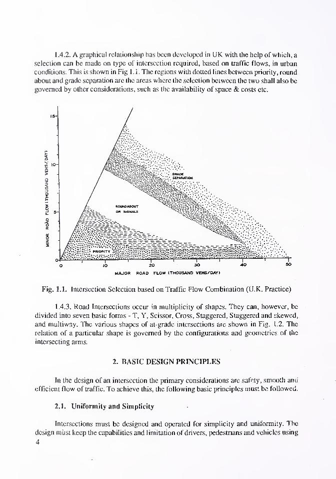
1.4.2. A graphical relationship has been developed in UK with the help of which, a
selection can be made on type of intersection required, based on traffic flows, in urban
conditions. This is shown in Fig 1.1. The regions with dotted lines between priority, round
about and grade separation are the areas where the selection between the two shall also be
governed by other considerations, such as the availability of space & costs etc.
MAJOR ROAD FLOW (THOUSAND VEHS/OAY)
Fig. 1.1. Intersection Selection based on Traffic Flow Combination (U.K. Practice)
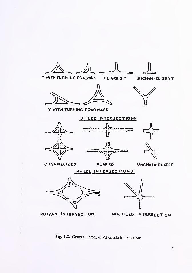
1.4.3. Road Intersections occur in multiplicity of shapes. They can, however, be
divided into seven basic forms - T, Y, Scissor, Cross, Staggered, Staggered and skewed,
and multiway. The various shapes of at-grade intersections are shown in Fig. 1.2. The
relation of a particular shape is governed by the configurations and geometries of the
intersecting arms.
2. BASIC DESIGN PRINCIPLES
In the design of an intersection the primary considerations are safety, smooth anu
efficient flow of traffic. To achieve this, the following basic principles must be followed.
2.1. Uniformity and Simplicity
Intersections must be designed and operated for simplicity and uniformity. The
design must keep the capabilities and limitation of drivers, pedestrians and vehicles using
4
T WITH TURNING ROADWAYS F L ARE 0 T UNCHANNEL I ZED T
Y WITH TURNING ROADWAYS
3- LEG INTERSECTIONS
CHANNELIZED FLARED UNCHANNE L I ZED
4- LEG INTERSECTIONS
ROTARY INTERSECTION MULTI LEG INTERSECTION
Fig. 1.2. General Types of At-Grade Intersections
5
intersection. It should be based on a knowledge of what a driver will do rather than what
he should do. Further all the traffic information on road signs and markings should be
considered in the design stage, prior to taking up construction work. All the intersection
movements should be obvious to the drivers, even if he is a stranger to the area. Complex
design which require complicated decision-making by drivers should be avoided. There
should be no confusion and the path to be taken by the drivers should be obvious.
Undesirable short cuts should be blocked. Further, on an average trip route, all the
intersections should have uniform design standards so that even a newcomer to the area
anticipates what to expect at an intersection. Some of the major design elements in which
uniformity is required are design speed, intersection curves, vehicle turning paths, super-
elevations, level shoulder width, speed change lane lengths, channelisation, types ofcurves
and type of signs and markings.
2.2. Minimise Conflict Points
2.2.1. Any location having merging, diverging or crossing manoeuvres of two
vehicles is a potential conflict point. Fig. 2.1 shows the potential conflict points for different
types of intersections. The main objective of the intersection design is to minimise the
number and severity of potential conflicts between cars, buses, trucks, bicycles and
pedestrians and whenever possible, these should be separated. This can be done by :
(i) Space separation by access control islands through channelising
(ii) Time separation : by traffic signals on waiting lanes.
Some of the common methods used to reduce conflict points are :
(a) Convert a 4-armed intersection having 32 conflict points to a roundabout having only 12 conflict
points. Round-about treatment may not, however, be warranted at most of rural locations except
those close to the urban areas.
(b) Signalise intersection. As Fig. 2.1 shows introduction of a two-phase signal reduces the conflict
points at 4 armed intersection from 32 to 16. If more phases are introduced and separate lanes
provided for turning traffic, conflict points can be virturally eliminated. (Provision of signals may
however, be justified only at a few rural locations carrying heavy traffic). Research abroad has
shown that signals increase accidents at simple intersections with low volumes but reduce them at
complex and/or high volume intersections.
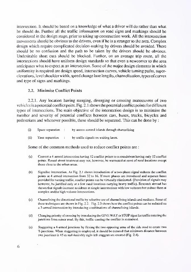
(c) Channelising the directional traffic by selective use of channelising islands and medians. Some of
these techniques are shown in Fig. 2.2. Fig. 2.3 shows how the conflict points can be reduced on
a 3-armed intersection by introducing combinations of channelising islands.
(d) Changing priority of crossing by introducing the GIVEWAY or STOP signs for traffic entering the
junctions from minor road. By this, traffic causing the conflict is restrained.
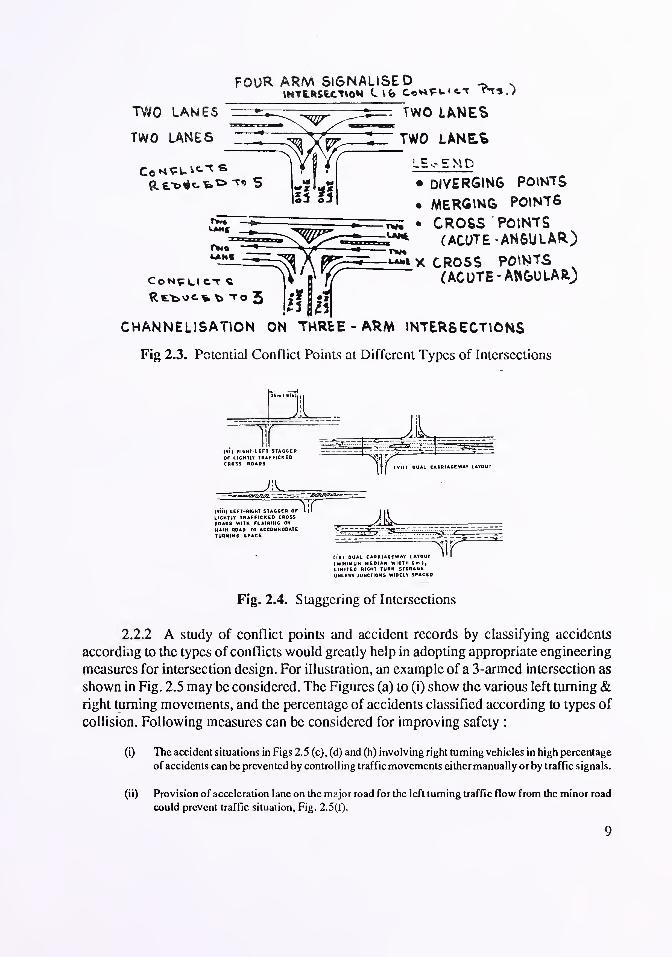
(e) Staggering a 4-armed junctions by flexing the two opposing arms of the side road to create two
T-junctions. When staggering is employed, it should be ensured that minimum distance between
two junctions is 45 m and desirably right-left staggers are created (Fig. 2.4).
6

Four arm non signalised Three -armintersection intersection
Round - about
—o-*
if—
Four- arm signalised
intersection
LEGENDo Diverging points
e Merging points
• Cross points (Acute-angular)
x Cross points (Right- angular)
Channelisation on three -arm intersection
Fig. 2.1. Potential Conflict Points at Different Types of Intersections
7

POUR ARM SIGNALISED _ .
INTERSECTION to«FUitt r-T5.;
TWO LANES
TWO LANES
TWO LANES
^ y^-Zrr TWO LANES
5 Si
C0N9LI CT «
Rtt>Ot% t> TO 3
• DIVERGING POINTS
• MERGING POINTS
7^ • CROSS POINTS(ACUTE -AN6ULAR)
^"X CROSS POINTS(ACUTE -ANGULAR.)
CHANNELISATION ON THREE - ARM INTERSECTIONS
Fig 2.3. Potential Conflict Points at Different Types of Intersections
(V|) RIGHT-LEFT STAGGEROF LIGHTLY TRAFFICKEDCROSS ROADS
(VIII) LEFT-RIGHT STAGGEL IGHT LY TRAFFICKED CROSSROADS WITH FL Al RING ON
MAIN ROAD TO ACCOMMODATETURNING SPACE
(IX) DUAL CARRIAGEWAY LAYOUT(MINIMUM MEDIAN WIDTH 6m),LIMITED RIGHT TURN STORAGEUNLESS JUNCTIONS WIDELY SPACEO
Fig. 2.4. Staggering of Intersections
2.2.2 A study of conflict points and accident records by classifying accidents
according to the types of conflicts would greatly help in adopting appropriate engineering
measures for intersection design. For illustration, an example of a 3-armed intersection as
shown in Fig. 2.5 may be considered. The Figures (a) to (i) show the various left turning &right turning movements, and the percentage of accidents classified according to types of
collision. Following measures can be considered for improving safety :
(i) The accident situations in Figs 2.5 (c), (d) and (h) involving right turning vehicles in high percentage
of accidents can be prevented by controlling traffic movements either manually or by traffic signals.
(ii) Provision of acceleration lane on the mpjor road for the left turning traffic flow from the minor road
could prevent traffic situation, Fig. 2.5(f)-
9

LEFT OUT LEFT IN
Mcye/ Road
(a) 07.
— MjruiY
( b) 0%
RIGHT OUT RIGHT IN
(c) 12% (d) 30%
COLLISION WITH ONCOMING VEHICLE
LEFT Q jY LEFT IN
(e) 6% tn 6%
RIGHT OUT RIGHT IN
(g) 9% (h) 157.
COLLISION WITH FOLLOWING VEHICLE
{') 22 7.
COLLISION BETWEEN TWO TURNING VEHICLE
Fig. 2.5. Analysis of Accident Types at Three Arm Intersections
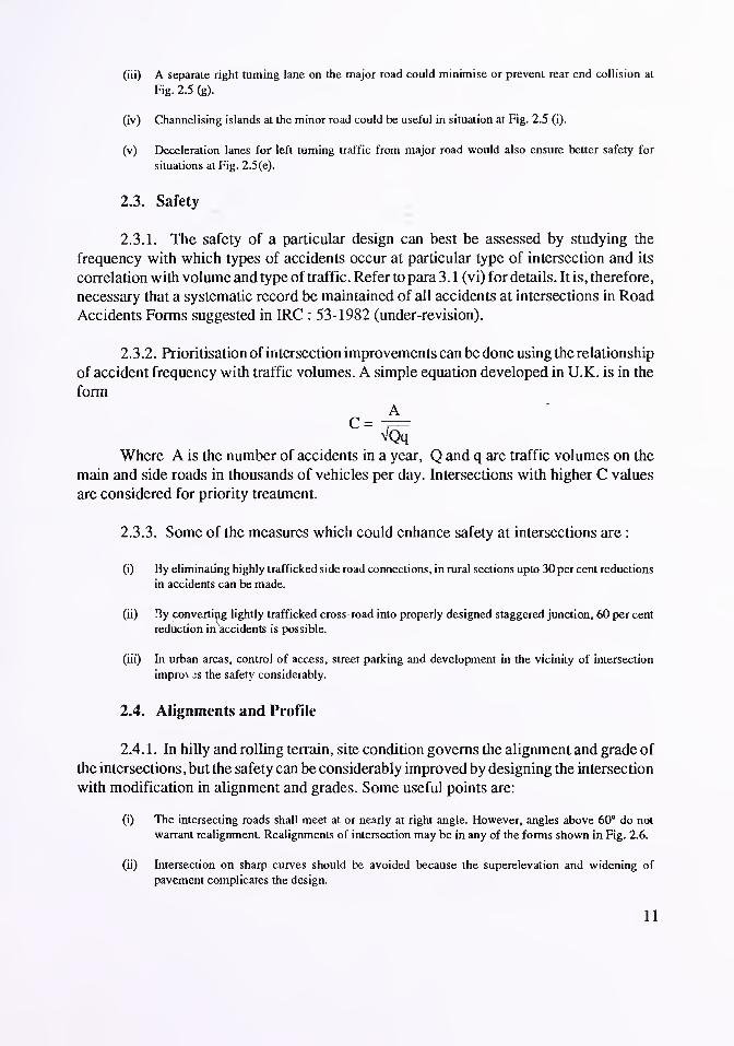
(iii) A separate right turning lane on the major road could minimise or prevent rear end collision at
Fig. 2.5 (g).
(iv) Channelising islands at the minor road could be useful in situation at Fig. 2.5 (i).
(v) Deceleration lanes for left turning traffic from major road would also ensure better safety for
situations at Fig. 2.5(e).
2.3. Safety
2.3.1. The safety of a particular design can best be assessed by studying the
frequency with which types of accidents occur at particular type of intersection and its
correlation with volume and type of traffic. Refer to para 3.1 (vi) for details. It is, therefore,
necessary that a systematic record be maintained of all accidents at intersections in Road
Accidents Forms suggested in IRC : 53-1982 (under-revision).
2.3.2. Prioritisation of intersection improvements can be done using the relationship
of accident frequency with traffic volumes. A simple equation developed in U.K. is in the
form
A~ VQq
Where A is the number of accidents in a year, Q and q are traffic volumes on the
main and side roads in thousands of vehicles per day. Intersections with higher C values
are considered for priority treatment.
2.3.3. Some of the measures which could enhance safety at intersections are :
(i) By eliminating highly trafficked side road connections, in rural sections upto 30 per cent reductions
in accidents can be made.
(ii) By converting lightly trafficked cross-road into properly designed staggered junction, 60 per cent
reduction in accidents is possible.
(iii) In urban areas, control of access, street parking and development in the vicinity of intersection
impro\ js the safety considerably.
2.4. Alignments and Profile
2.4. 1. In hilly and rolling terrain, site condition governs the alignment and grade of
the intersections, but the safety can be considerably improved by designing the intersection
with modification in alignment and grades. Some useful points are:
(i) The intersecting roads shall meet at or nearly at right angle. However, angles above 60° do not
warrant realignment. Realignments of intersection may be in any of the forms shown in Fig. 2.6.
(ii) Intersection on sharp curves should be avoided because the superelevation and widening of
pavement complicates the design.
11

12
Fig. 2.6. Realignment Variation of Intersection

(iii) Combination of grade lines or substantial grade changes should be avoided at intersection. The
gradient of intersecting highways should be as flat as practicable upto sections that are used for
storage space.
(iv) Grades in excess of 3 per cent should, therefore, be avoided on intersections while those in excess
of 6. per cent should not be allowed.
(v) Normally, the grade line of the major highway should be carried through the intersection, and that
of the cross road should be adjusted to it. This concept of design would thus require transition of the
crown of the minor highway to merge with the profile of the interface of major and minor roads (see
Fig. 2.7).
(vi) For simple unchannelised intersections involving low speed and stop signals or signs, it may be
desirable to warp the crowns of both roads into a plane at the intersection, the particular plane
depending on direction of drainage and other conditions.
(vii) Changes from one cross slope to another should be gradual. Intersection of a minor road with a
mullilane divided highway having a narrow median and :uperelevated curve should be avoided
whenever possible because of the difficulty in adjusting grades to provide a suitable crossing.
3. DESIGN DATA REQUIRED
3.1. In order to be able to properly design an intersection and give consideration to
factors affecting design, the following essential data must be collected :
(i) An index/location plan in the scale of about 1 : 10,000 to 1 : 20,000 showing the intersection under
consideration and the road/rail/rivernetwork in the area.
(ii) A base plan of the intersection site in the scale of 1 : 500. Where two or three intersections are located
close together, additional base plan to a scale of 1 : 1,000 should be prepared showing all the
intersections affected. It is important to maintain this scale which is being adopted as a measure of
uniformity and also to ensure that sufficient length of roads anc* fairly detailed account of existing
features are shown in a drawing sheet ofmanageable size. The existing roads and salient features like
road land boundary, location of structures trees, service lane etc., should be shown for a length of
about 200 m for each road merging at the intersections. If the terrain is not plain and/or there is too
much of variation of ground level at the site, contours at 0.5 metre interval should also be marked
on the base plan and additional longitudinal sections given along the centre line of intersecting
roads.
(iii) The peak hour design traffic data : The peak hour design traffic data should give its compositional
and the directional break-up. A sample proforma, which is to be used for the purpose of reporting
the compositional and directional break up and computing the volume in PCUs for one leg of a four
legged intersection, is given as Table 3.1
13

To be adiustad
to existing grade
INTERSECTION ON STRAIGHT
PLAN
LONGITUDINAli
Cross Slope
INTERSECTION ON INSIDE OF CURVE ON MAIN ROAD
In general it will be impracticable
to provide stopomg sight distance
(o the maior road pavementIn these cases the side road should
be graded up to edge oi formation
Ol the major road and a channelisingisland provided in the side roadapproach
LONGITUDINAL
Cross Slope
Local rounding
INTERSECTION ON OUTSIDE OF CURVE ON MAIN ROAD
Fig. 2.7. Main Road Intersections—Approach Grading on Side Roads
14

Table 3.1. Intersection Design Data
Intersection Design Data Peak Hour Hrs. To Hrs
Peak Hour Design Traffic
Name & Location of Intersection
From Leg A*
Entering LegB* Leg C* Leg D* Remarks
Type Nos PCUEqui-
valency
PCU Nos PCUEqui-
valency
Nos PCUEqui-
valency
1 2 3=1x2 1 2 1 2
Fast Vehicles
1. Passenger cars, tempos
auto rickshaw, tractors,
pickup vans
2. Motor Cycles, scooters
3. Agricultrual tractor Light
Commercial Vehicles
4. Trucks, Buses,
5. Tractor- Trailer, Truck
Trailer units
1.00
0.50
1.50
3.00
4.50
TOTAL FAST
Slow Vehicles
6. Cycles
7. Cycle Rickshaws
8. Hand Cart
9. Horse Drawn
10. Bullock-Carts
0.50
1.50
3.00
4.00
8.00
TOTAL SLOW
PEDESTRIAN Nos.
*Specify the name of an important place or land on this LEG such as Market LEG, Temple LEG, Mathura LEG, etc.
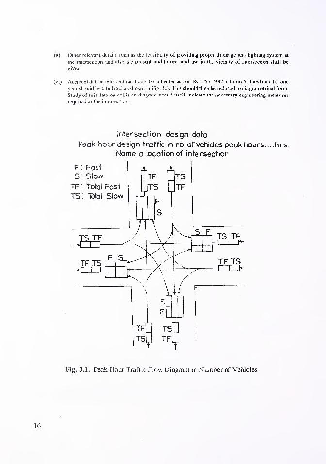
For converting vehicles into PCUs, equivalency factors given in Table 3. 1 should be used. Separate
report sheets will be needed for the other legs of the intersection. The volume of the above traffic in
terms of number of vehicles and in PCU should then be reflected in the diagrams shown in the Figs.
3.1 & 3.2. If the numbers of legs in the intersection are 3 or more than 4, these figures should be
suitably modified.
(iv) In the urban/sub-urban areas and intersection near villages with substantial pedestrian movements,
the peak hour data on persons crossing the intersecting road arms should be collected for the design
of a well planned pedestrian crossing facility at the intersection.
15
(v) Other relevant details such as the feasibility of providing proper drainage and lighting system at
the intersection and also the present and future land use in the vicinity of intersection shall be
given.
(vi) Accident data at intersection should be collected as per IRC : 53-1982 in Form A-l and data for one
year should be tabulated as shown in Fig. 3.3. This should then be reduced to diagrametrical form.
Study of this data ou collision diagram would itself indicate the necessary engineering measures
required at the intersection.
Intersection design data
Peak hour design traffic in no. of vehicles peak hours.
Name a location of intersection
hrs.
Fig. 3.1. Peak Hour Traffic Flow Diagram in Number of Vehicles
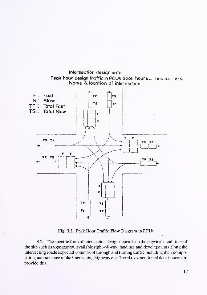
Intersection design data
Peak hour design traffic in PCUs peak hours.... hrs to....hrs.
Name & location of intersection
FS
TFTS : Total Slow
Fast
SlowTotal Fast
Fig. 3.2. Peak Hour Traffic Flow Diagram in PCUs
3.2. The specific form of intersection design depends on the physical conditions of
the site such as topography, available right-of-way, land use and developments along the
intersecting roads expected volumes of through and turning traffic including thek compo-
sition, maintenance of the intersecting highway etc. The above mentioned data is meant to
provide this.
17

>
PATH OF MOVING MOTORVEHICLE _
PEDESTRIAN PATHFATALNON FATALREAR END COLLISION -
LEGENDPARKED VEHICLE SFIXED OBJECTOVERTURNED «-*
OUT OF CONTROL
—
*
SIDESWIPE =>•
TIME — A* AM , P»PMPAVEMENT— D-DRY, I -ICY, W»WETWEATHER- C- CLEAR, F-FOO,R»RAIN
SL-SLEET, S-SNOW
ACCIDENT SUMMARY DAYLIGHT NIGHT TOTAL,CLASSIFICATION BY
TYPES FATAl| NONFATAl 0AJ1A
1
TOTAL
3
1
FATAlNONFATAl
PttOP.TOTAl FATAl
NON 'PROP.
FATAUOgw TOWl
APPROACHING AT RIGHTANOIf ' 1 1 2 2 ! 3 9
APPROACH**} SAME DIRECTION 1 1|2 2
APPROACHING OPP. DIRECTION 1 1 1 '
PEDESTRIAN ACCIDENTS 1 1 1 1 1
1
FIXED OBJECT ACCIOENTS
OTHER ACCIDENTS
TOTALS 2 3 3 1 3 4 3 6 9
Fig. 3.3. Collision Diagram
4. PARAMETERS OF INTERSECTION DESIGN
4.1. General
Intersections are designed having regard to flow speed, composition, distributic
and future growth of traffic. Design has to be specified for each site with due regard te
physical conditions of the site, the amount and cost of land, cost of construction and the
effect ofproposal on the neighbourhood. Allowances have to be made for space needed for
18
traffic signs, lighting columns, drainage, public utilities etc. The preparation of alternative
designs and comparison of their cost and benefits is desirable for all major intersections.
4.2. Design Speed
Three types of design speeds are relevant for intersection element design :
(i) Open highway or "approach" speeds
(ii) Design speed for various intersection elements. This is generally 40 per cent of approach speed in
built up areas and 60 per cent in open areas.
(iii) Transition speeds for design of speed change elements i.e. changing from entry/exit speed at the
intersection to merging/diverging speed.
The "Approach" speeds relevant to various types of terrain and roads are given in
Table 4.1 and 4.2 respectively.
In rural areas ruling design speed should be used, but minimum can be adopted in
sections where site conditions and costs dictate lower speeds. In urban areas a lower or
higher value ofdesign speed can be adopted depending on the pressure of physical controls,
roadside developments and other related factors. A lower value is appropriate for central
business areas and higher in sub-urban areas.
4.3. Design Traffic Volumes
Intersections are normally designed for peak hour flows. Estimation of future traffic
and its distribution at peak hours is done on the basis of past trends and by accounting for
factors like new development of land, socio-economic changes etc . Where it is not possible
to predict traffic for longer period, intersection should be designed for stage development
for design periods in steps of 10 yrs. Where peak hour flows are not available they may be
assumed to be 8 to 10 per cent of the daily flow allocated in the ratio of 60: 40 directionally.
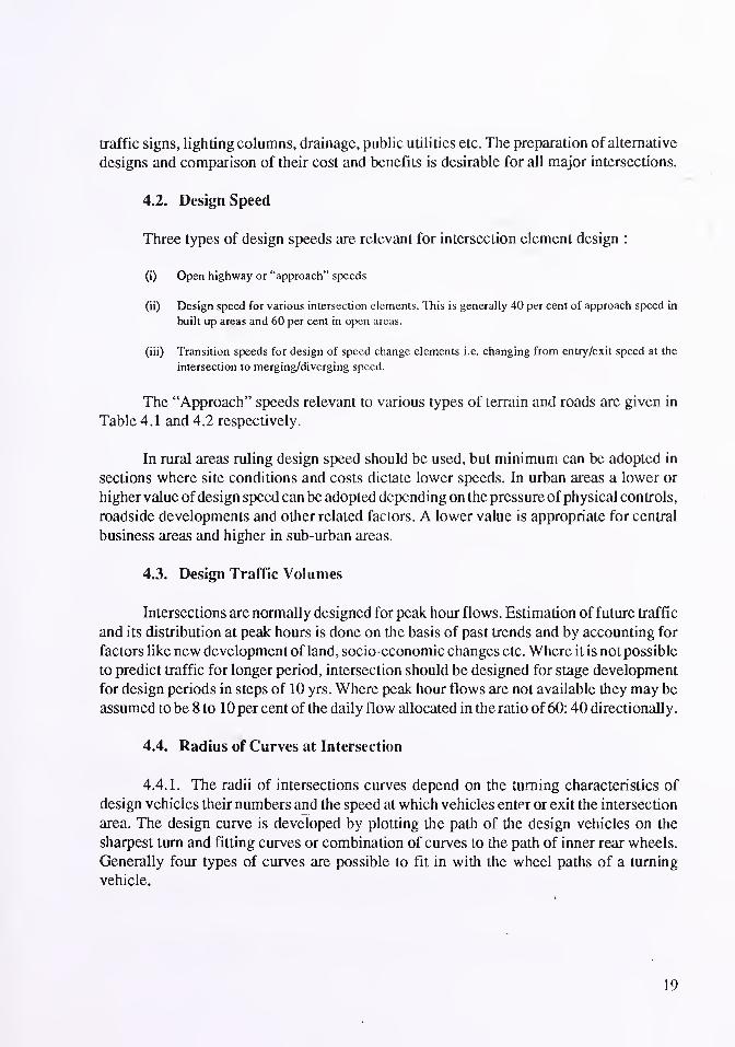
4.4. Radius of Curves at Intersection
4.4.1. The radii of intersections curves depend on the turning characteristics of
design vehicles their numbers and the speed at which vehicles enter or exit the intersection
area. The design curve is developed by plotting the path of the design vehicles on the
sharpest turn and fitting curves or combination of curves to the path of inner rear wheels.
Generally four types of curves are possible to fit in with the wheel paths of a turning
vehicle.
19
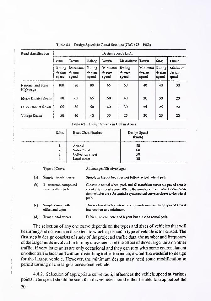
Table 4.1. Design Speeds in Rural Sections (IRC : 73 - 1980)
Road classification Design Speeds km/h
Plain Terrain Rolling Terrain Mountainous Terrain Steep Terrain
Ruling
design
speed
Minimumdesign
speed
Ruling
design
speed
Minimumdesign
speed
Ruling
design
speed
Minimumdesign
speed
Ruling
design
speed
Minimumdesign
speed
National and State
Highways
100 80 80 65 50 40 40 30
Major District Roads 80 65 65 50 40 30 30 20
Other District Roads 65 50 50 40 30 25 25 20
Village Roads 50 40 40 35 25 20 25 20
Table 4.2. Design Speeds in Urban Areas
S.No. Road Classifications Design Speed
(km/h)
1. Arterial 80
2. Sub- arterial 60
3. Collection street 50
4. Local street 30
Type of Curve
(a) Simple circular curve
(b) 3 - centered compound
curve with offsets
(c) Simple curve with
offset and taper
(d) Transitional curves
Advantages/Disadvantages
Simple in layout but does not follow actual wheel path
Closest to actual wheel path and all transition curve but paved area is
about 20 per cent more. Where the numbers of semi-trailer combina-
tion vehicles are substantial a symmetrical curve is closer to the wheel
path.
This is closest to 3- centered compound curve and keeps paved area at
intersection to a minimum
Difficult to compute and layout but close to actual path.
The selection of any one curve depends on the types and sizes of vehicles that will
be turning and decision on the extent to which a particular type of vehicle is to be used. The
first step in design consists of study of the projected traffic data, the number and frequency
of the larger units involved in turning movement and the effect of those large units on other
traffic. If very large units are only occasional and they can turn with some encroachment
on other traffic lanes and without disturbing traffic too much, it would be wasteful to design
for the largest vehicle. However, the minimum design may need some modification to
permit turning of the largest occasional vehicle.
4.4.2. Selection of appropriate curve radii, influences the vehicle speed at various
points. The speed should be such that the vehicle should either be able to stop before the
20
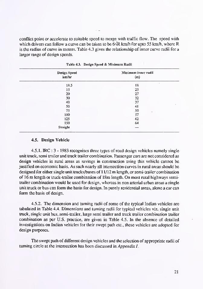
conflict point or accelerate to suitable speed to merge with traffic flow. The speed with
which drivers can follow a curve can be taken to be 6VR km/h for upto 55 km/h, where Ris the radius of curve in meters. Table 4.3 gives the relationship of inner curve radii for a
larger range of design speeds.
Table 43. Design Speed & Minimum Radii
Design Speed Minimum inner radii
km/hr (m)
18.5 18
15 23
20 27
30 32
40 37
50 41
75 50
100 57
125 62
150 64
Straight
4.5. Design Vehicle
4.5.1. IRC : 3 - 1983 recognises three types of road design vehicles namely single
unit truck, semi trailer and truck trailer combination. Passenger cars are not considered as
design vehicles in rural areas as savings in construction using this vehicle cannot be
justified on economic basis. As such nearly all intersection curves in rural areas should be
designed for either single unit trucks/buses of 1 1/12 m length, or semi-trailer combination
of 16 m length or truck-trailer combination of 18m length. On most rural highways semi-
trailer combination would be used for design, whereas in non arterial urban areas a single
unit truck or bus can form the basis for design. In purely residential areas, alone a car can
form the basis of design.
4.5.2. The dimension and turning radii of some of the typical Indian vehicles are
tabulated in Table 4.4. Dimensions and turning radii for typical vehicles viz. single unit
truck, single unit bus, semi-trailer, large semi trailer and truck trailer combination trailer
combination as per U.S. practice, are given in Table 4.5. In the absence of detailed
investigations on Indian vehicles for their swept path etc., these vehicles are adopted for
design purposes.
The swept path of different design vehicles and the selection of appropriate radii of
turning circle at the intersection has been discussed in Appendix I.
21

4.5.3. There are five common situations in design of intersections and each one has
to be generally designed for following conditions :
S.No. Location of Intersection
1. Rural Section
2. Suburban Arterial Section
3. Urban Arterial & Sub-Arterials
4. Urban Central Business Districts
5. Residential area
Curve Design
Design for single unit truck is preferredfor intersection with
local minor roads. Semi-trailer design is preferred for major
road intersection where large paved areas result, channelisa-
tion also becomes essential.
Designed for semi-trailer with speed change lanes and chan-
nelisation. Three-centered compound curves are preferred.
Designed for single unit truck
Designed for single unit trucks forminimum curve radii with
allowance for turning vehicles encroaching on other lanes.
Designed for cars only with encroachment of tracks into
other lanes.
Table 4.4. Dimensions and Turning Radii of Some of the Typical Indian Vehicles
S.No. Make of Vehicle Length
(m)
Width
(m)
Turning Radius
(m)
1. Ambassdor 4.343 1.651
2. Maruti Car 3.300 1.405 4.400
3. TATA (LPT 2416)
3-axled truck
9 010 2.440
4. TATA (LPO 1210)
Full forward control
Bus chasis
9.885 2.434 10.030
5. TATA (LPO 1616)
Bus chasis
11.170 2.450
6. Leyland Hippo Haulage 9.128 2.434 10.925
7. Leyland (18746)
Taurus
8.614 2.394 11.202
8. Leyland
Beaver Multi Drive
12.000 2.500
9. Mahindra Nissan
Allwyn Cabstar
5:895 1.870 6.608
10. Swaraj Mazda Truck (WT 49) 5.974 2.17(5 6.400
11. DCM Toyota (Bus) 6.440 1.995 6.900
22
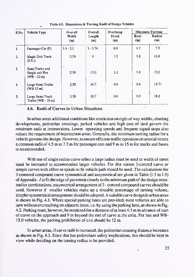
Table 4.5. Dimensions & Turning Radii of Design Vehicles
S.No. Vehicle Type Overall Overall Overhang Minimum Turning
WiH thTT 1U 111
(m)
T AtiotH
(m)
Front
(m)
Rear
(m)
Radius
(m)
1. Passenger Car (P) 1.4-2.1 3 - 5.74 0.9 1.5 7.3
2. Single Unit Truck
(S.U.)
2.58 9 1.2 1.8 12.8
3. Semi Trailer and
Single unit BusAvn i o _\^wts - iz m)
2.58 15.0 1.2 1.8 12.2
4. Large Semi-Trailer
(WB-15m)2.58 16.7 0.9 0.6 13.71
5. Large Semi-Truck
Trailer (WB - 18 m)
2.58 19.7 0.6 0.9 18.2
4.6. Radii of Curves in Urban Situations
In urban areas additional conditions like restriction on right of way widths, abutting
developments, pedestrian crossings, parked vehicles and high cost of land govern the
minimum radii at intersections. Lower operating speeds and frequent signal stops also
reduce the requirement of intersection areas. Generally, the minimum turning radius for a
vehicle governs the design. However, to ensure efficient traffic operation on arterial streets
a common radii of 4.5 m to 7.3 m for passenger cars and 9 m to 15 m for trucks and buses
is recommended.
With use of single radius curve either a large radius must be used or width of street
must be increased to accommodate larger vehicles. For this reason 3-centred curve or
simple curves with offset or spirals to fit vehicle path should be used. The calculations for
3-centered compound curve symmetrical and assymetrical are given in Table (1-3 to 1-5)
ofAppendix -I to fit the edge of pavement closely to the minimum path of the design semi-
trailier combinations, assymetrical arrangement of 3 - centred compound curves should be
used. However if smaller vehicles make up a sizeable percentage of turning volume,
simpler symmetrical arrangement should be adopted. A suitable curve design in urban areas
is shown in Fig. 4.1. Where special parking lanes are provided, most vehicles are able to
turn without encroaching on adjacent lanes, i.e. by using the parking lane, as shown in Fig.
4.2. Parking must, however, be restricted for a distance of at least 4.5 m in advance of start
of curve on the approach and 9 m beyond the end of curve at the exist. For bus and WB-15.0 vehicles, the parking prohibition of exit should be 12 m.
In urban areas, if curve radii is increased, the pedestrian crossing distance increases
as shown in Fig. 4.3. Since this has pedestrians safety implications, this should be kept in
view while deciding on the turning radius to be provided.
23

(A) TWO SPIRALS ( B) COMPOUND CURVE
(R« 6i», 9m, 10.3m) (Hi !9,TO J«,)
ac/cc AB/OE!B
BF/aor
"l «l 0 ti ac/ce AB/ DE Bf/ Oc
10.5 m J9.I40 15. 190 3.950 10 3 31.5 5V 17.5 m 9.33" 1.42
3 m 16.830 13.290 3.5*o 1 27 5** 15 m 8' 1.22
6 m 11 22 Oj ft . 860 2 340 6 18 18* 5*" 10 n 5. 33* 081
Fig. 4.1. Design of Streel Lanes Curve
4.7. Width of Turning Lanes at Intersection
Determination of widths of turning lanes at intersection is primarily based upon the
type of vehicles using it, the length of lanes, the volume of traffic and if kerbs are provided,
the necessity to pass a stalled vehicles. Table 4.6 gives the recommended widths of turning
lanes. These can be assumed to have a capacity of 1200 PCU/hr.
Table 4.6. Width of Lanes at Intersections
Inner Design Single Single lane width Two lane width
Radius'f
speed lane width with space to pass for one or two
km/h. m stationary vehicles way traffic
,v , m m
(1) (2) (3) (4)* (5)
10.5 18 5.50 10.53 11.5
15 23 5.50 9.50 10.5
20 27 5.00 9.00 10.0
30 32 4.50 8.00 9.0
40 37 4.50 7.50 9.00
50 41 4.50 7.00 8.00
75 50 4.50 7.00 8.00
100 57 4.50 7.00 8.00
125 62 4.50 6.50 8.00
150 64 4.50 6.50 8.00
4.50 6.00 7.00
These widths are applicable for longer slip roads (over 60m length) and should be used only if vehicles are
allowed to park.
24

WB- IS DESIGN VEHICLE -v .^-o-nC CROSS STR
*^T ^ \.-tf*"~>>J*US
WB-12
PARKING LANE -'JPAVEMENT EDGE
% CROSS STREET WB-t'S DESIGN VEHICLE
>3i# PARKING RESTRICTION FOR SU* PARKING RESTRICTION FOR WB-12
WB~ 50 AND BUS
Fig. 4.2. Effect of Kerb Radii and Parking on Turning Paths
25
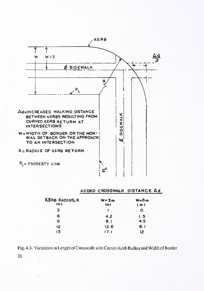
KERB
rrW W/2
j£ SIDEWALK
AdsINCREASED WALKING DISTANCEBETWEEN KERBS RESULTING FROMCURVED KERB RETURN ATINTERSECTIONS
Wa WIDTH OF BORDER OR THE NOR- ',
MAL SETBACK ON THE APPROACHTO AN INTERSECTION
Rs RADIUS OF KERB RETURN
PL= PROPERTY LINE
ADDED CROSSWALK DISTANCE Ad
K&RB RADIUS, R W-3m W=6m((D) (ml ( m )
3 1 06 4.2 1. 59 8. 1 4.5
12 12.6 8. 1
15 17. 1 12
Fig. 4.3. Variations in Length of Crosswalk with Corner-Kerb Radius and Width cf Border
26

4.8. Auxiliary Lanes
Three types of auxiliary lanes are provided at intersections. These are storage lanes,
right turning lanes, acceleration lanes and deceleration lanes. The last two together are also
called speed change lanes. Provision of these increases the capacity of intersection and
improves safety. The length of these lanes depends on the volume of traffic entering or
leaving the side road. The shape of these can be either parallel lane with sharp taper or a
direct taper or with a transition curve. Fig. 4.4 shows the method of introducing addition
lane using transition curves.
4.8.1. Storage lanes/right turning lanes : Storage lanes are generally more important in
urban areas where volume of right turning traffic is high and if not catered for, blocks the
through traffic. Normal design procedure provides for storage length based on 1 .5 times the
average number of vehicles (by vehicle type) that would store in turning lane at peak hour.
At the same time the concurrent through lane storage must also be kept in view, as it mayhappen that entry to turning lane may become inaccessibile due to queued vehicles in
through lane. Fig. 4.5 shows several methods of introducing turning lane at intersections.
Figs. 4.6 and 4.7 show satisfactory method of widening at intersections and widening for
turning lanes at intersections.
Example of Design
Consider an urban intersection with angle, right turn lane and the through lanes with
a signal installed with a cycle time of 90 sec. Assume (he right turn traffic volume at design
peak hour to be 150 vehicles (10 trucks) and through volume to be 520 vehicles (15%trucks). The storage lane length is determined as follows :
60x60No. of cycles per hour = x 40
90
150No. of right turning vehicles per cycle = ~~~ = say 4
520and No. of through vehicles per cycle per hour = ——— = say 7
Assuming the peak traffic within the hour to be uniform (if this is not so further
adjustment will be required) the length of lanes, using a truck adjustment factor and car
length of 7.5 m (Ambassador car) and truck length of 1 lm, lane length is determined as
below.
Length of right turn lane = 4 x 0.9 x 7.5 + 4 x 0.1 x 1 1 = 31.4 m
Length of through lane = 7 x 0.85 x 7.6 + 7 x 0.15 x 1 1 = 56.17 m
Choose design length of storage lane = 56 m.
27

28
Fig. 4.5. Provision of Turning Lanes at Intersections
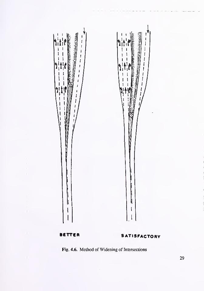

Fig. 4.7. Method of Widening for Turning Lanes at Intersections

In places where not more than one or two vehicles are expected to wait for right turn,
such as in rural areas, the storage lane may be provided as per Table 4.7.
Table 4.7. Length of Right Turning Lane
Design Speed Length of storage lane
(km/h) including 30 • 45 m taper
(m)
120 200
100 160
80 130
60 110
50 90
4.8.2. Speed Change Lanes : Speed change lanes are more important in rural areas. In
urban areas such lanes are rarely required but provision of short lanes to assist merging and
diverging manoeuvres are provided in conjunction with channelising islands. Speed
change lanes should are uniformly tapered and have a set back of 5.4 m at the tangent point
of curve leading into or out of minor road. The turning lane should be reduced in width to
4.25 m by carriageway marking etc. as shown in Fig. 4.8.
Acceleration lanes
An acceleration lane should be designed so that vehicles turning left from the minor
road may join the traffic flow on the major road at approximately the same speed as that
of the nearside lane traffic in the major road. Acceleration lanes also improve capacity by
enabling the use of short traffic gaps and by providing storage space for traffic waiting to
merge when large traffic gaps occur. Acceleration lanes are recommended where the future
traffic on the acceleration lane is accepted to be more than 1,000 PCU's per day.
U—30-»omTAM» »i
u
Fig. 4.8. Typical Dimensions of Road Intersections
31

Recommended lengths of acceleration lanes for different main road design speeds
are given in Table 4.8 and a typical layout is given in Fig. 4.8. In difficult conditions sub-
standard lengths may have to be accepted, but these should not be less than half of those
recommended.
Table 4.8. Minimum Acceleration Lane Lengths
Highway Acceleration Length (m)
for entrance curve design speed (kmph)
Stop 25
conditions
30 40 50 60 65 75 80
Design
Speed
(kmph)
Speed
Reached
(kmph)
and initial speed (kmph)
0 20 30 35 40 50 60 65 70
50 40 60
65 50 120 100 75 70 40
80 60 230 210 190 180 150 100 50
100 75 360 340 330 300 280 240 160 120 50
110 85 490 470 460 430 400 380 310 250 180
Table 4.9. Minimum Deceleration Lane Length
Highway
Design
Speed
(kmph)
Average
Running
Speed
(kmph)
Deceleration Length (m)
For Design Speed of Exit Curve
Stop
condition
25 30 40 50 60 65 75 80
for Average Running Speed of Exit Curve
0 20 30 35 40 50 60 65 70
50 45 70 60 50 40
65 60 95 90 80 70 60 50
°80 70 130 120 120 110 100 90 70 50
100 85 160 150 150 140 130 125 100 90 70
105 90 175 165 160 150 150 130 120 100 85
110 95 190 180 175 170 160 150 130 120 100
Where acceleration lanes are on a down gradient their length may be reduced to
1-0.08G times the normal length, where G is the gradient expressed as a percentage.
Deceleration Lanes
Deceleration lanes are of greater value than acceleration lanes because the driver of
a vehicle leaving the highway has no choice but to slow down any following vehicles on
32

the through lane if a deceleration lane is not provided. Deceleration lanes are needed on the
near side for left turning traffic and on the right turn lane where provision is made for right
turning traffic.
The length of near side deceleration lanes should be sufficient for vehicles to slow
down from the average speed of traffic in the near side lane to the speed necessary for
negotiating the curve at the end of it; in order to make deceleration lanes effective, the curve
radius must permit a speed of at least 30-40 kmph (not less than 30 m). Recommendedlengths of near side deceleration lanes are given in Table 4.9 and a suitable layout is given
in Fig. 4.8. Near side deceleration lanes are recommended for intersection on roads where
the future traffic on the deceleration lane is expected to be more than 750 p.c.u's/day.
Where the number of traffic lanes on a road is reduced immediately beyond a slip
road, in order to avoid entrapping through vehicles in the slip road the carriageway should
be constructed to full width to the exit nose and a taper length of 180 m provided beyond
it.
Right-turn deceleration lanes in the central reserve should be provided at all gaps for
right-turning traffic on dual-carriageway roads. On three-lane roads, the centre lane should
be marked tor right turning traffic where the product of estimated future cutting flows in
p.c.u's/per day is more than one million. The widening of two-lane single-carriageway
roads to > rovide right-turn deceleration lanes in the centre of the road should be considered
at the same levels of flow as for three-lane roads. These provisions may be made for lessser
flows where accident records warrant them , or on two-lane roads where they can readily be
incorporated in realignment or other scheme. On overloaded three lane roads or where the
road junction is on a crest, it is usually desirable to construct short lengths of dual
carriageways and provide right-turn deceleration lanes for right-turning traffic.
The lengths ofright-turn deceleration lanes should be sufficient for vehicles to slow
down to a stop from the average speed of vehicles in the off side lane omission of these
lanes will usually result in numerous head to tail collisions. These lanes should not be
less than 3 m wide and parallel-sided with entry and return radii of 180 m giving a taper of
30 -45 m.
Even if it is not practicable to provide the full length of deceleration lane (right-turn
or nearside) sub-standard lengths are still of great benefit but they should not be less than
half the recommended lenghts.
Where deceleration lanes are on an up-gradient their length may be reduced to
that obtained by multiplying the recommended length by 1 — 0.03G whereas G is the
gradient expressed as a percentage. For deceleration lanes on a down gradient their length
may be increased that obtained by multiplying the recommended length by 1 + 0.06G.
33
4.9. Super Elevation and Cross-slope
Where the turning slip lanes are provided for higher speed operation at intersection,
they should be superelevated for the appropriate speed as given in the appropriate
geometric design standard (Fig. 4.9) The principle of superelevation runoff also applies.
But in intersection design the actual curves are of limited radii and length. As such in
practice it is difficult to provide the required superelevation without causing abrupt cross-
slope change, whiducould be dangerous. In practice therefore lower rates of supereleva-
tion are often accepted to intersections to maintain riding comfort, appearance and to effect
a balance in design. The cross slopes in the intersecting area should be maintained as per
IRC : 73 - 1980. In the intersection area normally the pavement cross-slope should be
carried through to the turning lanes as well to avoid creation of drainage problem.
Extreme care must be exercised to check the drainage of the entire intersection area
and cross-over crown lines. Where necessary drainage inlets should be designed and so
located as to minimise the spread of water on traffic lanes and eliminate stagnant pools in
the intersection area. No sheet flows should be allowed across the intersection where
pavement surface are warped and surface water should be intercepted before the change in
cross-slope. Also inlets should be located upgrade of pedestrian crossing so that the
pedstrian crossings are always free of water.
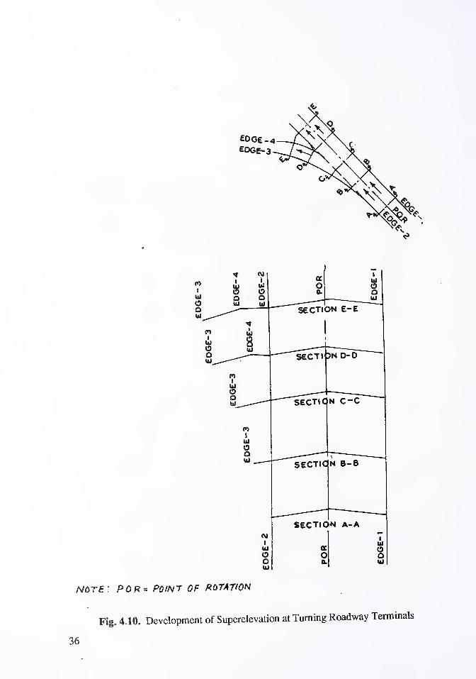
At turning lanes of intersection, superelevation commensurate with radii and speed
is seldom possible as too great a difference in cross-slope may cause vehicles changing
lanes and crossing crown line to go sideways with possible hazard. When high-bodied
trucks cross the crown line at some speed at an angle of about 10° to 40°, the body throw
may make vehicle control difficult and may result in overturning. The method of
developing superelevation of turning lanes for different situations is illustrated in Fig. 4.10
to 4.13.
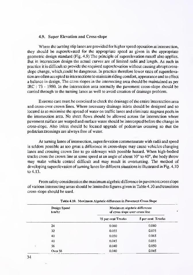
From safety consideration the maximum algebric difference in pavement cross slope
of various intersecting areas should be limited to figures given in Table 4.10 and transition
cross-slope should be used.
Table 4.10. Maximum Algebric difference in Pavement Cross Slope
Design Speed Maximum algebric difference
km/hr of cross slope over cross line
75 per cent Trucks 5 per cent Trucks
24 0.060 0.080
32 0.055 0.075
40 0.050 0.065
40 0.045 0.055
56 0.040 0.050
Over 56 0.040 0.045
34

§ft,!
(HldM U3d 3ai3W> NDIlW\3-|3a3driS
35
36
note: por* Point of Rotation
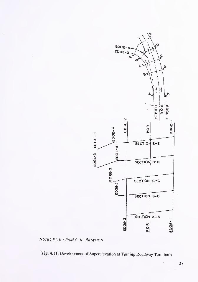
Fig. 4.11. Development of Superelevation at Turning Roadway Terminals

an
ou
nc
sectionI o-o
SECTION c-c
SECTION 8-8
SECTION a-A
I
Ooui
NOTE'. POR POINT OF DOTATION
Fig. 4.12. Development of Superelevation at Turning Roadway Terminals
38

NOTE : POR ' POINT OF ROTATION
Fig. 4.13. Development of Superelevation at Turning Roadway Terminals
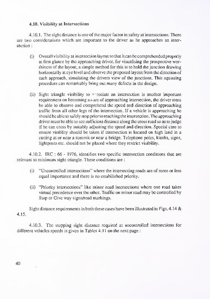
4.10. Visibility at Intersections
4.10.1. The sight distance is one of the major factor in safety at intersections. There
are two considerations which are important to the driver as he approaches an inter-
section :
(i) Overall visibility at intersection layout so that it can be comprehended properly
at first glance by the approaching driver, for visualising the prospective wor-
thiness of the layout, a simple method for this is to hold the junction drawing
horizontally at eye level and observe the proposed layout from the direction of
each approach, simulating the drivers view of the junctions. This squinting
procedure can remarkably bring out many defects in the design.
(ii) Sight triangle visibility to " c'otiate an intersection is another important
requirement on becoming aware of approaching intersection, the driver must
be able to observe and comprehend the speed and direction of approaching
traffic from all other legs of the intersection. If a vehicle is approaching he
should be able to safely stop prior to reaching the intersection. The approaching
driver must be able to see sufficient distance along the cross road so as to judge
if he can cross by suitably adjusting the speed and direction. Special care to
ensure visiblity should be taken if intersection is located on high land in a
cutting at or near a summit or near a bridge. Telephone poles, kiosks, signs,
lightposts etc. should not be placed where they restrict visibility.
4.10.2. IRC : 66 - 1976, identifies two specific intersection conditions that are
relevant to minimum sight triangle. These conditions are :
(i) "Uncontrolled intersections" where the intersecting roads are of more or less
equal importance and there is no estabilished priority.
(ii) "Priority intersections" like minor road intersections where one road takes
virtual precedence over the other. Traffic on minor road may be controlled by
Stop or Give way signs/road markings.
Sight distance requirements in both these cases have been illustrated in Figs. 4. 14 &4.15.
4.10.3. The stopping sight distance required at uncontrolled intersections for
different vehicles speeds is given in Tables 4.1 1 on the next page :
40

VISIBILITY AT INTERSECTIONS
0|P tJ#| ftTOUPWI 8IOMT PlItAHCI *"
OtfTIUCTien -\l a*.
Fig. 4.14. Minimum Sight Triangle at Uncontrolled Intersections
7^MAJOR ROA6
rzB—f
[fl-UCONDI »«» DKTANCCfC0»CSr0H01M TO KflllMWHO OP TMf MAJOR WAS
c.BOO ROAO
1
Note:- Any obstruction should be cleor of the m.mmutr. vt^tbtlity triangle
fof a htijht of i-Zm above the t-oadway.
Fig. 4.15. Minimum Sight Triangle at Priority Intersections
Table 4.11. Safe Stopping Sight Distance of Intersections
Speed Safe stoping Sight Distance
(m)
20 10
25 25
30 30
40 45
50 60
60 80
65 90
80 130
1J0 180
41

For priority intersections IRC : 66-1976 recommends a minimum visibility of 15 malong the minor road while for the major road, sight distance equal to 8 seconds travel at
design speed is recommended. Visibility distances corresponding to 8 seconds travel time
are set out below in Table 4.12.
Table 4,12. Visibility Distance on Major Roads
Design Speed Minimum Visibility Distance
(km/h) along major road (m)
100 270
80 180
65 145
50 110
All sight distance obstructions, like bushes, trees and hoardings in the visibility
triangle should be removed to improve safety. Fig. 4.16 shows the desirable amount of
trimming to be done to hedges and trees at intersections.
TRIM YOUR HEDGE
BUSHES AND TREES FOR
safety's SAKE
Fig. 4. 16. Trimming of Trees and Hedges Required for Clear Sight Distance
42

4.11. Channelising Island
4.1 1.1. The objectives of providing channelising island are to :
(i) control speed and path of vehicles at the intersection ;
(ii) control angle of conflict
;
(iii) separate conflicting traffic streams ;
(iv) provide shelter to vehicles waiting to carry out certain manoeuvres;
(v) assist pedestrians to cross;
(vi) reduce excessive carriageway areas and thus limit vehicle paths; and
(vii) locate traffic control devices.
The general types of island and their shapes are shown in Fig. 4.17. To ensure
proper functioning of each type of islands, principles given below for each should be
adhered to
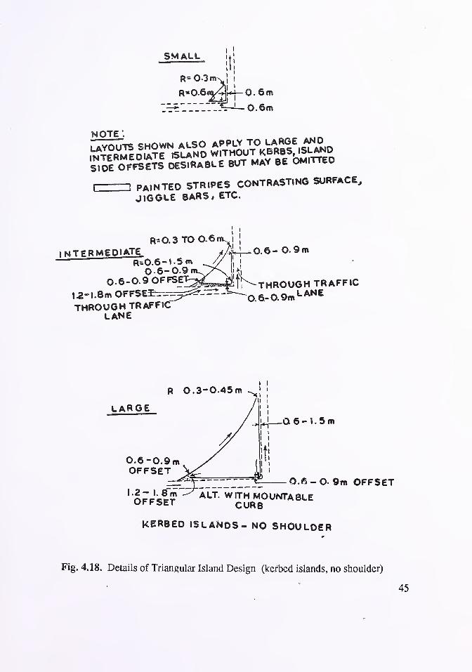
4.11.2. Corner or directional islands : Figures 4.18 to 4.20 illustrate the design
features of corner islands and the considerations which govern their sizes and
shapes. Corner or Directional Islands (normally triangular) should meet the following
requirements
:
(a) It should be of sufficient size to be readily identified and visible. For an island to be clearly seen it
must have an area of at least 4.5 m2in urban areas and 7 m2 in rural areas and should usually be
bordered with painted raised kerbs. Smaller areasmay be defined by pavementmarking Accordingly
triangular islands should not be less than 3.5 m and preferably 4.5 m on a side after rounding of
curves.
(b) It should be offset from normal vehicle path by 0.3 m to 0.6 m. The layout should be tested using the
track diagram for all turning movements (Fig. 4.21).
(c) It should be provided with illuminated sign or a ballard at suitable places e.g. apexes of islands. It
should be of sufficient size to enable placement of such traffic control devices.
(d) It should be accompanied by suitable carriageway marking to show actual vehicle paths. Marking
should be made conspicuous by use of reflectorised materials.
(e) It should be properly marked for night visibility.
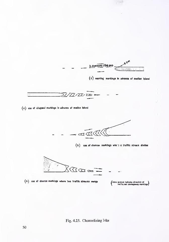
4.11.3. Centre or divisional islands : Centre islands requires careful location and
designing. They require careful alignment and are invariably accompanied by widening of
right-of-way as illustrated in Fig. 4.22. Centre or divisional islands should meet the
following requirements
(a) It should be preceeded by a clearly marked or constructed natural area of not less than 1 .5 sec. travel
time at approach speed (Fig. 4.23).
43

44
Fig. 4.17. General Types and Shapes of Islands
SMALL
NOTE".
SIDE OFFSETS DESIRABLE BUT MAY BE OMITTED
r-1 POINTED STRIPES CONTRASTING SURFACE,
JIGGLE BARS, ETC.
R--0.3 TO O.61
1 INTERMEDIATE *L
Rx0.6- 1 5 mO 6-0 9
0. 6-0.9 OFFSET^l2-l.8mOFFSE5rrr--rr
THROUGH TRAFFICLANE
0.6- 0 9m
THROUGH TRAFFIC
0.6-0.9m LANE
R 0.3-0.45m ^LARGE
0.6-0.9mOFFSET
06- 1.5m
— _\_ZZZ~ZZZ1jz—
°
(
L£~'f-f?
~ ALT WITH MOUNTABLEOFFSET CURB
KERBED ISLANDS- NO SHOULDER
- 0- 9m OFFSET
Fig. 4.18. Details of Triangular Island Design (kerbed islands, no shoulder)

SMALL
06m OFFSET
NOTE.
LAYOUTS SHOWN ALSO APPLY TO LARGE ANDINTERMEDIATE ISLANDS WITHOUT KERBS,ISLAND
SIDE OFFSETS DESIRABLE BUTMAY BE OMITTED
^^^SHOULDER
0.3-0.4
INTERMEDIATE
R 0.3 -<X9m
0.3-O9m OFFSET-
THROUGH TRAFFICLANE
0.6-0- 9m
THROUGHTRAFFICLANE
m -N
0.6- 0.9m OFFSET 0.6.0.9|!
»4-0- 6- 0.9 m
KERBED WITH SHOULDERS
Fig. 4.19. Details of Triangular Island Design (kerbed island with shoulders)

SINGLE UNIT TRUCK PATHOUTER RADIUS 2 lint
WB- 50 SEMITR. COH8. PATHOUTER RADIUS 22.5 m t
-CENTERED CURVE ^C/O<?m-ISm-45m OFFSET 1.5m >
EQUIVALENT SIMPLE CURVE RADIUS 21m
_ B-
0.6m
Fig. 4.20. Design for Turning Roadways with Minimum Corner Island

(if (0
Fig. 4.21. Methods of Offsetting Approach Nose of Channelising Island
(b) It should be offset by about 1.5 m to 3 m from edge of main carriageway and suitably offset from
approach centreline based on the track diagram of all turning movements (Fig. 4.24)
(c) It should be preceded by longitudinal and vertical profile which provides atleast the minimumacceptable sight distance.
(d) It should present a smooth, free flowing alignment into and out of the divided road.
(e) It should have excess width of pavement at the nose to create a "funnel effect".
(f) It should have sufficient length to warn drivers of the approaching intersection. A 3 sec. driving time
of approach speed is sufficient.
(g) It should be sufficient width to permit use of bullet nose design with adequate right turn radii for
vehicles and to permit placement of traffic control devices.
(h) It should not be less than 1.2 m wide and 6 m length. In special cases width can be reduced to
0.6 m.
The island shape is determined by wheel track diagram of vehicles using the road,
the radii of left and right turns, island nose radii, approach pavement widths, general
geometry of island and excess space to be covered by the island. Fig. 4.25 shows the correct
method ofshaping the centre traffic island while Fig. 4.26 shows the shapes of traffic island
for different angles of turning. Fig. 4.27 shows the details of design of a divisional island.
Fig. 4.28 shows the correct method of shaping a central island. The decision to provide an
island or not should be based on examination of volume of traffic especially buses/trucks
and the estimation of the probability of actual number of conflicts caused by right turning
vehicles encroaching upon the stop position of vehicles on the intersecting road. In less
volume rural roads or in residential streets, non-channelised intersection may be con-
structed as the few conflicts will not give economic justification for full fledged channel-
ised intersection.
48

49
3.gnttntrkj.ftlftjjgp
(s) warning markings In advanea of median Island
(4) use or diagonal markings In advance of median Island
!
(s) use of chevron markings whe j a traffic stream divides
I
!
(g) use of chevron markings where two traffic streams merge /not.: arrow* indicate dir.etlon of \
\ traf f ic. not carriageway markings/
50
Fig. 4.23. Channelising Islai

Fig. 4.24. Offset Details of Central Islands
ft
f
CORRECT SATISFACTORY INCORRECT
Fig. 4.25. Shaping the Traffic Island
51

OS o ifct
toc
e
5
00
bOC<
|
Pt-H
T3
t/3
O
t-i
HObOC
C3
SO
TT
52

RAISED TRANSITION APPROA- RAISED MEDIAN ISUCH TO ISLAND-COLOR AND WITH KERBSTEXTURE CONTRASTING WITH r*-po rNORMAL PAVE MC NT
PLAN
MEDIAN ISLAND AREA PREE£RGRASSED
SLOPING CURB EXCEPTATPEDESTRIAN CROSSING
ABLY
of highway
ormal pavement
SECTION AT P.T. ( P0 ,NT 0F TAPER)
RAISED TRANSITION APPROACHTO lSLAND;COLOR AND TEX-TURE CONTRASTING WITHNORMAL PAVEMENT
NORMAL PAVEMENT
MEDIAN ISLAND AREAP«EF£RABLY GRASSED
KERB
SECTION BETWEEN P.T. AND P.R.C.
RAISED TRANSITION APPROACHTO ISLAND- COLOR AND TEX-TURE CONTRASTING WITHNORMAL PAVEMENT HIGH POINT
SECTION AT P. R.C. ( POINT OF RAISED CARRIAGEWAY)
DIAGRAMMATIC CROSS SECTIONS
Fig. 4.27. Details of Divisional Island Design
53

(1) WRONG
Fig. 4.28. Correct Method of Shaping a Central Island
4.11 .4. Pedestrian refuge island : IRC : 70-1977 "Guidelines on Regulation and Control
of Mixed Traffic in Urban Areas", provides general guidance on placement of pedestrian
refuge island in urban areas. According to IRC : 103-1988, "Guidelines for Pedestrian
Facilities", central refuges may be considered if the carriageway exceeds 4-lanes. The
width of central refuge shall be 1.5m and above depending on the crossing pedestrian
volume and space available. The refuge island should be provided with vertical kerb which
should be suitably reflectorised and illuminated.
4.12. Considerations in Island Designs
4. 12. 1 . An important point to be considered in island design is that its outline should
be immediately obvious. It should be of easy flowing curved lines or straight lines parallel
to the line of travel. Driver should not be confronted suddenly with unusable area and the
island first reached should be indicated by gradually widening marking or a conspicously
roughned strip that directs traffic to one side at easily traversed speeds. Multiple islands
should be avoided and a few large islands should be preferred. It may be advisable to any
temporary layouts of movable kerbs or send bags and observe traffic with several variation
before designing and constructing a permanent island.
4.12.2. The use of kerbed island should be reserved for multi-lane highways or
streets and for the more important intersections on two lane roads. In or near urban areas
where speeds are low, drivers are accustomed to confined facilities and fixed lighting is
possible, channelisation can be used freely. However, high unmountable kerbs with rigid
angle-iron frames should not be used as they pose danger to life and property.
4. 12.3. Where divisional islands are provided, approach roads should be so widened
as to smoothly cater to all the directional traffic movement, see Figs. 4.5, 4,6 & 4.7. Thealignment should be such that no undue effort in vehicle steering is required.
4.12.4. Drainage of highway after the introduction of island should be ensured.
Large islands should be depressed inside to avoid draining across the pavement. Small
islands can be mounted where pavement cross-slopes are outwards.
4.12.5. Island can be formed in three ways :
(1) raised island outlined by kerbs
(2) island delineated by pavement marking, buttons or raised rumble strips placed on all paved areas
(3) non-paved areas formed by the pavement edge supplemented by delineations or a mounded earth
treatment beyond the pavement edge.
4.12.6. Typical layout of a T-intersection showing progressive use of islands to
channelise traffic as dictated by increasing traffic is shown in Fig. 4.29. Fig. 4.30 shows
typical details of channelises for a right hand splay junction.
55
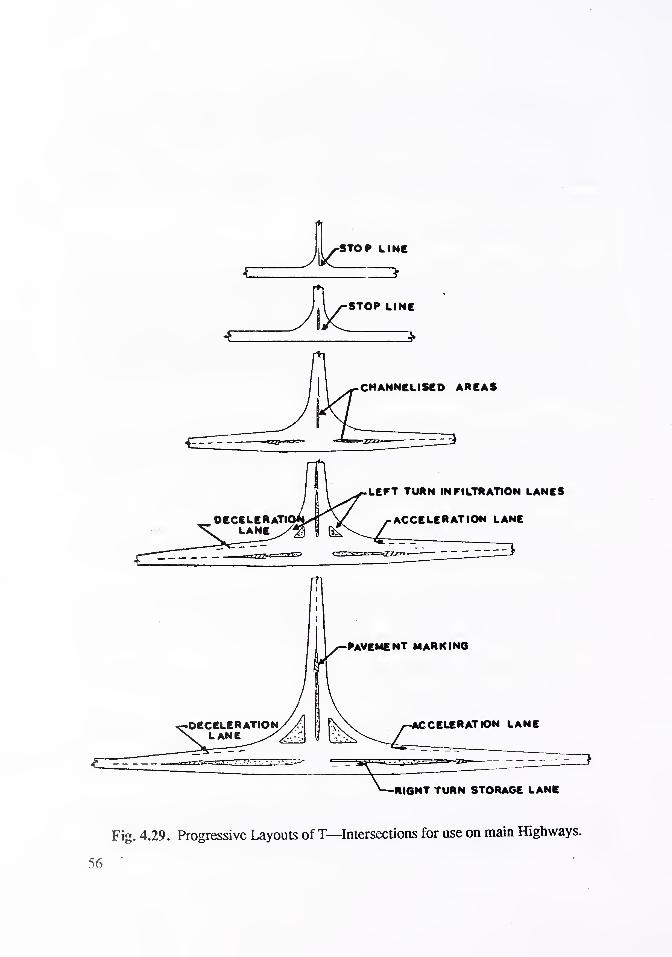
STOP LINE
STOP LINE
CHANNELISED AREAS
LEFT TURN INFILTRATION LANES
ACCELERATION LANE
RIGHT TURN STORAGE LANE
Fig. 4.29. Progressive Layouts ofT—Intersections for use on main Highways.
56

Fig. 4.30. Type Layout of a Right Hand Splay Intersection
4.12.7. A layout of four-leg intersection providing simultaneous right turns for a
main road with a bullet nose is indicated in Fig. 4.31.
4. 12.8. Gap in central island ofjunctions : To permit easy right turning of large vehicles,
the gap in central reserve ofjunction should be extended to at least 3m beyond the assumed
extension of kerb line of minor road and shape should be determined by 12 to 15m radius
control circles tangential both in the centre line of minor road and the major road as shown
in Fig. 4.24. To facilitate turning, the ends of the central island should be bullet nosed.
Where a median right turn lane is to be accommodated, the design should be as shown in
Fig. 4.32.
57

4- LA N OIVJOED-Qsn MEDIAN
. rr""z sskp . / v \ ^^^^
2~ LAN E 1!
I1
Fig. 4.31. Four-arm Intersection Providing Simultaneous Right Turns
4.13. Kerb
It is desirable to provide kerbs at the intersections in urban and sub-urban area.
Kerbs may be barrier type, semi-barrier type or mountable type as shown in Fig. 4.33.
Appropriate situations for use of each type are given in IRC : 86-1983 on "Geometric
Design Standards for Urban Roads in Plains". The kerbs where used should be mountable
type except for pedestrian refuge where they should be non-mountable.
4.14. Traffic Rotary
A traffic rotary is a specialised form of at-grade intersection where vehicles from the
converging roads are forced to move around an island in one direction in an orderly and
regimented manner and "weave" out of the rotary movement into their desired directions.
The details of design of traiuc rotaries are covered in IRC : 65-1976, "Recommended
Practice for Traffic Rotaries.''
58

mCoTan
THROUGH-TRAFFIC LAW6S-
—
M 3" 3 .6mt -a-
'3.36 m
—^-THROUGH— ~—TRAFFIC LANCS
3
iE
-V, CROSS STRiEET
tit—
M = MGDlAN WIDTH
L ~ LEHCTH OF MEDIAN OPENING
R= CONTROL RADIUSPROVIDED IN ACCORDANCE WITH PARA 4.12.8
1
—g—
s
(6) Semi-barrier type
Fig. 4.33. Typical Kerb Sections
p—aso—
^
(c) Mouniable type
All dimensions in millimetres
59
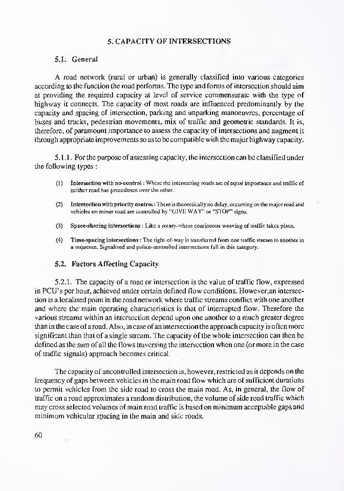
5. CAPACITY OF INTERSECTIONS
5.1. General
A road network (rural or urban) is generally classified into various categories
according to the function the road performs. The type and forms of intersection should aim
at providing the required capacity at level of service commensurate with the type of
highway it connects. The capacity of most roads are influenced predominantly by the
capacity and spacing of intersection, parking and unparking manoeuvres, percentage of
buses and trucks, pedestrian movements, mix of traffic and geometric standards. It is,
therefore, of paramount importance to assess the capacity of intersections and augment it
through appropriate improvements so as to be compatible with the major highway capacity.
5.1.1. For the purpose of assessing capacity, the intersection can be classified under
the following types
:
(1) Intersection with no-control : Where the intersecting roads are of equal importance and traffic of
neither road has precedence over the other.
(2) Intersection with priority control : There is theoretically no delay, occurring on the major road and
vehicles on minor road are controlled by "GIVE WAY" or "STOP" signs.
(3) Space-sharing intersections : Like a rotary-where continuous weaving of traffic takes place.
(4) Time-spacing intersections : The right-of-way is transferred from one traffic stream to another in
a sequence. Signalised and police-controlled intersections fall in this category.
5.2. Factors Affecting Capacity
5.2.1. The capacity of a road or intersection is the value of traffic flow, expressed
in PCU's per hour, achieved under certain defined flow conditions. However,an intersec-
tion is a localised point in the road network where traffic streams conflict with one another
and where the main operating characteristics is that of interrupted flow. Therefore the
various streams within an intersection depend upon one another to a much greater degree
than in the case of a road. Also, in case ofan intersection the approach capacity is often more
significant than that of a single stream. The capacity of the whole intersection can then be
defined as the sum of all the flows traversing the intersection when one (or more in the case
of traffic signals) approach becomes critical.
The capacity of uncontrolled intersection is, however, restricted as it depends on the
frequency of gaps between vehicles in the main road flow which are of sufficient durations
to permit vehicles from the side road to cross the main road. As, in general, the flow of
traffic on a road approximates a random distribution, the volume of side road traffic which
may cross selected volumes of main road traffic is based on minimum acceptable gaps and
minimum vehicular spacing in the main and side roads.
60

5.2.2. The capacity of an intersection depends on the following factors :
(1) Physical and operating conditions :
(a) Width of approach,
(b) One way or two way operation,
(c) Parking conditions/Ribbon development.
(2) Traffic Characteristics :
(a) Turning Movements
(b) Percentage of trucks & buses
(c) Local factors at signalised intersection (ratio of the number of green phases that are fully
utilised by traffic during peak hour to the total number of green phases available for that
approach during the same period,
(d) Peak hour factors (ratio between the number of vehicles counted during the peak hour and
four times the number of vehicles counted during the highest 15 consecutive minute).
(e) No. of Pedestrians and Cyclists crossing the intersection.
(a) Location
(b) Control Measures
(i) Traffic Signals and Signs
(ii) Marking of approach lanes
5.2.3. In India, very little data is available on actual estimates of capacities of
intersection under mixed traffic conditions. The basic approach in evaluating capacity is to
estimate traffic flows theoretically and then to modify the results based on actual
information and identify factors which affect capacity. A further development in this
direction is simulation modelling of traffic behaviour of intersection - so as to capture gap-
acceptance behaviour and handways etc.
5.3. Capacity Determination
5.3.1. It may be noted that, due to the likely wide variations in local conditions,
single level-of-service values and capacities cannot be presented even in situations having
similar geometries. A simple approach for capacity assessment of at-grade intersections is
given in Appendix-II. For signalised intersection, a simple method based on U.K. practice
is recommended in Chapter -7. Another approach based on Highway Capacity Manual of
U.S.A. and research done in India is given in Appendix-Ill, which can be used after
carefully understanding the procedure.
5.3.2. Intersection capacity should be equal to the capacity of the approach
roads. The design capacity of 2-lane one way road may be taken to vary from 1400 to 2400
PCU's/hour (i.e. 700 to 1200 PCU's/ hour/lane). On a 2—lane two way road, capacity is
900 to 1500 PCUs/hour (i.e. 450 to 750 PCU's/hour/lane). In estimating the approach road
capacity thought should also be given to road classification e.g. an arterial road is expected
to have higher capacity than a sub-anerial or collector road.
61

5.3.3. In spite of all the difficulties inherent in estimating capacities of intersection,
it can be confidently said that the following measures will improve the capacity of an
intersection
:
(1) On Major Roads
(a) Addition of acceleration and deceleration lane,
(b) Separation of two directions of traffic by a median, thus allowing crossing in two stages,
(c) Provision of separate storage lane for turning traffic.
(2) On Minor Road :
(a) Channelisation,
(b) Increasing number of lanes available, particularly the right and left turns.
5.3.4. Capacity changes from the separation of conflicts : The principle of Separating traffic
conflicts can be applied both to grade separated intersections and at- grade intersections.
Separation of conflicts by the application of signal controls is more appropriate to urban
or fringe urban areas. The capacity can also be augmented by fixing priority for the major
road at intersections.
6. USE OF TRAFFIC CONTROL DEVICES AT INTERSECTIONS
6.1. Types of Devices
In intersection design, the possible use of traffic control devices and other road
furniture should be considered. The common types of traffic control devices which are
helpful in reducing accidents and improving flow conditions at intersections are road
markings, road signs, signals, railing and flashing lights.
6.2. Road Markings
Carriageway markings within and in the neighbourhood of an intersection restrict
vehicles from using areas other than those actually meant for them and thus ensure orderly
movement of traffic. Depending on the actual intersection conditions, carriageway
markings of intersections may consist of one or more of the followings :
(i) Centre line-solid or broken;
(ii) Solid centre lines preceded by broken centre lines on approaches to important intersections as an
additional aid to channelise traffic ;
(iii) Centre line along with barrier lines;
(iv) Turn markings;
(v) Directions markings; and
(vi) Lane markings
Fig. 6.1 illustrates typical carriageway markings of road intersections. For more
details, IRC 35 : 1970 (under revision) may be referred. In choosing the type of markings,
62
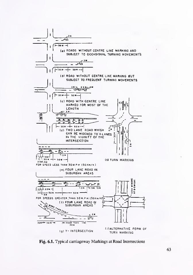
J«L_
0 J ROADS WITHOUT CENTRE LINE MARKING ANDSUBJECT TO OCCASIONAL TURNING MOVEMENT'S
rTft?
( b) ROAD WITHOUT CENTRE LINE MARKING HUTSUBJECT TO FREQUENT TURNING MOVEMENTS
(c) ROAD WITH CENTRE LINEMARKED FOR MOST OF THELENGTH3 M-
.
m 1
6* I
1— SOU--)— SOM—~|
(d) TWO LANE ROAD WHICHCAN BE WIDENED TO 4 LANES oIN THE VICINITY OF THEINTERSECTION
7^
fjAJ—!
J .
—FOR SPEED LESS THAN 30M.PH (50 Km/hi
(e) FOUR LANE ROAD IN
I SUBURBAN AREAS
(h) TURN MARKING
MORF THANION
(g) Y - INTERSECTION( i ) ALTERNATIVE FORM OF
TURN MARKING
Fig. 6.1. Typical carriageway Markings at Road Intersections
63

discretion should be exercised by judiciously, considering the conditions at site where the
lane markings are to be provided, care must be taken to ensure continuity of lanes across
the intersection.
6.3. Signs and Signals
To properly guide and control the traffic approaching junctions, traffic signs and
signals are installed. IRC : 67-1977 "Code of Practice for Road Signs" provides a more
detailed description of various traffic signs and their applications. Design and provisions
of traffic signals has been dealt separately under section 7 of these guidelines. While
providing traffic signs at intersection, due care mu^t be taken to ensure the effectiveness of
the sign posted. It should always be noted that too many signs with inadequate spacing maybecome totally ineffective and at times result in confusion and -accidents. Some of the
traffic signs which are useful in guiding/regulating the traffic at intersections are shown in
Fig. 6.2. For other details on their sizes and colour codes, IRC : 67-1977 may be referred.
The posting of traffic signs must be done with adequate care so that they perform their
intended function most effectively, in as much as the sign must be posted ahead of the spot
to which it refers. When more than one sign is to be posted, they should be adequately
separated in space so as to be seen one at a time and convey the message with complete
effect Signs with reflective properties (preferably retro-reflective type) must be used so as
to meet the requirements of night traffic.
While posting the signs, adequate care should be taken so as to avoid the chance of
their causing obstruction to pedestrian and vehicular traffic. In urban areas the lowest edge
of any traffic sign should not be lower than 2.1m from the pavement when posted on foot-
paths/side walks. In rural areas the clear height ofsign from the edge ofthe pavement should
be 1.5 m. The nearest edge of the sign should be at least 1.2 m away from the edge of the
carriageway on rural roads. When posted on raised foot-paths the same should be away by
at least 30 cm from the edge of the kerb.
A few typical examples of posting traffic signs at urban and rural intersections are
illustrated in Figs. 6.3 to 6.6.
6.4. Reflectors
A large percentage of accidents at intersections occur at night due to poor visibility
and hazards like traffic islands, median openings or other objects close to the carriageway.
At such locations, use of reflector units of suitable dimensions can improve safety
considerably. A typical unit suitable for use on island consists of three circular reflective
units mounted on triangular plate as per IRC : 79-1981. In urban or sub-urban areas, safety
is best improved by illuminating the entire intersection area adequately.
6.5. Railings
The requirements of railings at intersection have been dealt in IRC : 103-1988
"Guidelines for Pedestrians Facilities" which may be referred to for more details.
64

ROAD SIGNS AT INTERSECTIONS
STOP SIGN
LEFT TURNPROHIBITED
11ACROSSROAD
Y -INTER-
SECTION
REGULATORY /MANDATORY SIGNS
VGIVE WAY NO ENTRY
U-TURNPROHIBITED
CHANGE LANEP ROHIBITED
ONE - WAY
0SPEEDLIMIT
WARNING SIGNS
12
SIDEROAD
A AY- INTER-
SECTION
ASIDEROAD
Y- INTER-
SECTION
14
T - INTERSECTION
A AMAJOR ROAD MAJOR ROAD
AHEAD AHEAD
STAGGEREDINTERSECTION
PEDESTRIANCROSSING
INFORMATORY SIGNS
58
* m2 ,
Dt-^' 81
24
25
RIGHT TURNPROHIBITED
10
NOPARKING
15
ROUNDABOUT
A ASTAGGEREDINTERSECTION
26
Fig. 6.2. Signs Used at Intersections
65
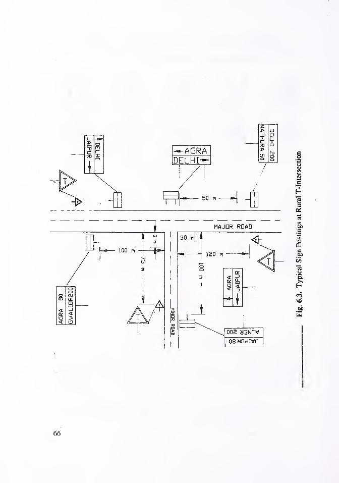

DELHI 30
MEERUT 20
001
002 andivr
Fig. 6.4. Typical Sign Posting at Rural Four Arm Intersection (Four-Arm Intersections)
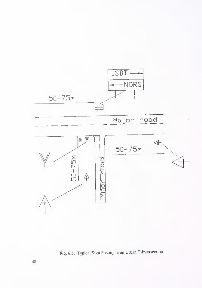
ISBT—-— NDRS
-75m
0Major road
_
Fig. 6.5. Typical Sign Posting at an Urban T-Intersection
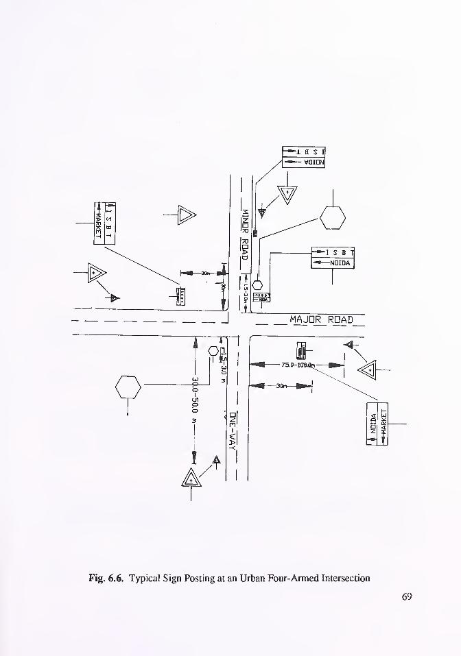
Fig. 6.6. Typical Sign Posting at an Urban Four-Armed Intersection

7. SIGNAL CONTROLLED INTERSECTION
7.1. The primary aims of signal control at an intersection are :
(i) To reduce traffic conflicts and delay,
(ii) To reduce accidents,
(iii) To economise on police time.
7.2. Warrants for Traffic Signal Installation
Before the traffic design process can commence, it must be determined whether or
not the volume of traffic entering the intersection warrants signalisation.
The need for a traffic control signal at any intersection must be evaluated in relation
to the following warrants :
Warrant 1 - Minimum Vehicular Volume,
Warrant 2 - Interruption of continuous traffic,
Warrant 3 - Minimum pedestrian volume,
Warrant 4 - Accident experience,
Warrant 5 - Combination of Warrants.
The traffic control signals should not be installed unless one or more signal warrants
as discussed in Section III of IRC : 93-1985 "Guidelines on Design and Installation ofRoadTraffic Signals" are met. The satisfaction of a warrant, however, does not always
completely justify signal installation. Engineering judgement must be exercised to ensure
that the signal could not increase the hazards or cause unnecessary delay.
7.3. Traffic Survey
The initial step may consist of a quick review of existing volume data and accident
records. A field visit to the location is necessary to observe the existing conditions and
intersection geometry. At those locations where further study appears justified, the next
step is to schedule and plan the engineering studies appropriate to the particular location
which will indicate whether more detailed data is required for signal design and plan
preparation if a signal is warranted.
A comprehensive investigation of traffic conditions and fiscal characteristics of the
location is essential to determine the necessity for a signal installation and to furnish
necessary data for the appropriate design and operation of signal that is warranted. The
advance traffic and engineering data required have been discussed in Section III- 1 of IRC:
93-1985.
7.4. Geometric Design
70Following parameters are to be considered.

7.4.1. Selecting approach widths : Because signals permit traffic movement from any
approach for only a portion of the time it is sometimes necessary for the intersection
approaches, where queuing takes place to be wider than the roads which feed these
approaches in order to pass the required flow (Figs. 7.1, 7.2 and 7.3 refers). In selecting
approach widths one criteria which can be used is the minimisation of the area occupied by
the intersection.
For a normal two phase cross roads, approach width (WtandW
2as in Fig. 7.1) should
be proportionate to the square roots of the ratio of flows, qj and q2respectively. The green
times (gt , g2)and length of widened road (d,, d
2)(as in Fig. 7.1) should be in the same ratio
as the width Wx&W
2respectively.
^ = _£i_ = A = J~Kw, g, d
2" *
q.
Where
qp q2 = maximum flow in PCU in phases 1 & 2 respectively.
q = flow i.e. the average number of vehicles passing a given point on the road in the same direction
per unit time.
Phase = , State of signals during which a particular stream or group of streams receives right of way.
Fig. 7.1. Simplified Diagram of Widened Approaches at Signal Controlled Intersection
71

TWO 7 mCARRIAGEWAYS
1.2 m CENTRALRESERVATION
TOTAL_ WIDTH
16 m BULGE TO DIRETOFF SIDE THROUGHTRAFFIC INTOCENTRE LANE
GUIDANCE MARKINGSFOR TURNING VEHICLES
WIDENING BY 1 ft.
1 THIN LINES SHOWORIGINAL LAYOUT )
NOT TO SCALE
Fig. 7.2. Suggested Layout for Offset Central Reserve
TWO LANES 7.0m
CARRIAGEWAYSJ.
THREE 10.50mLANES
1.2 m CENTRALRESERVATION
TOTAL WIDTH16.0 m
TWO LATOTAL
19.0 m
BULGE TO DIRECTOFF SIDE THROUGHTRAFFIC INTOCENTRAL LANE
GUIDANCE MARKINGSFOR TURNING VEHICLES
LOCAL WIOENI NG BY
( THIN LINES SHOWORIGINAL LAYOUT )
NOT TO SCALE
Fig. 7.3. Offset Central Reserve with Improved Visibility for Right Turning Vehicles
Thus a major road carrying four times as much traffic as its minor cross road should
have approaches which are twice as wide as the minor approaches and should have green
times twice as long.
For T-intersections with two phase control the ratios of width, green times and
lengths widened should be :
= -vT^and ...(2)
W2
y 2q2
72

where the suffix 2 refers to the minor cross road. Thus a major road through a
T-intersection carrying four times as much traffic as the minor cross road should have a
width 1.4 times than that of cross road, a length of widening 2.8 times and a green period
2.8 times as long as that of a minor cross road.
7.4.2. The flow can be determined by a census of all traffic using the intersection
over a day including all peak periods. Calculations should cover morning, evening and
other peaks to determine the predominant flows at different times of the day. The width
required for any approach not considered may be determined from the green time allotted
to its phase. In deciding the values of q land q2
for substitution in the above formula, right
turning vehicles if few in number should be taken as equivalent to 1.75 of straight ahead
vehicles. If right turning volume is large enough to require special right turn lanes this
should be substracted from the flow q xand q2
before determining the ratios of remaining
approach widths.
Where uniform widening of an approach is prevented by the presence of existing
buildings, it may only be possible to flare the approach. On dual carriageway roads extra
width may sometimes be obtained by reducing the width of the central reserve.
7.43. Selection of lane widths : It is normal to have lanes 3 m wide at new or improved
intersections, through occasionally 2.8 m lanes may have to be accepted at existing
intersections because of site constraints. A lane width of 3.4 m or 3.6 m may be
warranted where traffic includes a larger- proportion of commercial vehicles. Where there
is a high proportion of bicycles it may be beneficial to have a wider (upto 4.0 m) near side
lane.
Approach widths may need to be adjusted to provide appropriate integral number of
lanes for straight through and turning traffic, having regard to the overall width available.
Where the approach width is less than 5.5 m no lane markings should be provided; for
widths between 5.5 m and 7.5 m the approach should be marked two lanes; for widths
between 7.5 m and 9 m the approach should be marked as three lanes. All lane width need
not be the same and should be chosen with regard to the volume and type of traffic using
each lane.
7.4.4. Layout for right-turning vehicles : Opposing right-tumings traffic can turn either
on the off side of each other or on the near side. If the near side method of turning right is
used there may be advantages in off setting the central line or central reserve, so that morespace is available to traffic approaching the intersection than to traffic leaving it. For
exceptionally high flow ofright turning vehicles, it is sometimes necessary to provide morethan one lane for them with separate phase. A separate phase should be provided if there
73

are many right turners from both approaches using near side method of turning. In some
cases it may be desirable to place the opposing right turners opposite each other as in
Fig. 7.2. Layout suggested in Fig. 7.3 improves visibility for right turners and facilitates the
signalling of the right turners if they move on a separate phase.
If right turning traffic from one approach is heavy, the green period of this approach
may continue after the end of green period of the opposing arm sharing the same phase
(Fig. 7.4).
The layout shown in Fig. 7.5 includes a pedestrian crossing which is a usual nature
of intersection where there are appreciable number of pedestrians. A pedestrian refuge is
usually placed at or near the centre of a single carriageway if the widths available to traffic
in the two directions are greater than 4.0 m.
N N N
PHASE B PHASE A
Fig. 7.4. Early Cut-off
7.5. Signal Design
Determination ofcycle lengths and green periods in signal phasing alongwith typical
design of signal timings are discussed in Section 11(22) of IRC : 93-1985.
74

PEDE S TRIAN CROSSING
REFUSE ISLANO
TRAFFICSIGNAL
STOP LINE
KERB LINE
illinium-t S T 0 P
w
0
FOOTPATH
EFFECTIVE APPROACHROAD WIDTH
I
BARRIER LINE
LANE LINEMARKING
NOT TO SCALE
Fig. 7.5. Typical Intersection Approach Road Showing Pedestrian Crossing
7.6. Intersection Capacity
The amount of traffic that can pass through a signal control intersection from a given
approach depends on the green time available to the traffic and on the maximum flow of
vehicles past the stop time during the green periods. The capacity and service volume that
a signalised intersection can handle depends upon geometries, signal operation and traffic
factors. The capacity of a signalised intersection can be determined from the expression :
Capacity = (g X s)/c vehicles per hr.
Where g = effective—green time in seconds
s = the saturation flow (vehicle per hr.)
c = cycle time in seconds.
These parameters can be determined as follows :
7.6. 1 . Saturation flow :The saturation flow is the flow which would be obtained if there
is a continuous queue of vehicles and they were given 100 per cent green time. It is
generally expressed in vehicles per hour of green time. When the green period
75

commences, vehicles take some time to start and accelerate to normal running speed but
after a few seconds the queue discharges at a more or less constant rate which is called
saturation flow. This concept is explained in Fig. 7.6 wherein the effective green time has
been explained through which the flow is assumed to take place at saturation rate and a lost
time during which no flow takes place. The curve in Fig. 7.6 can be replaced by a rectangle
of equal area where the height of the rectangle is equal to the saturation flow. Saturation
flow can be estimated by the following methods :
AREA UNDER SOLIO CURVE = g x s
SATURATION FLOW —
S
GREEN AMBER RED
Fig. 7.6. Saturation Flow and Lost Time
7.6.1.1. Approach width : The saturation flow(s) expressed in terms of Passenger CarUnits (PCUs) per hr. and with no parked vehicles present is given by
s = 525 (w) PCUs per hr.
where w = width of approach road in m. measured from kerb to the inside ofthe central median or centre
line of the approach whichever is nearer.
This expression is valid for widths from 5.5 m to 18 m. For a lesser width the values
may be obtained from the table given on next page :
76
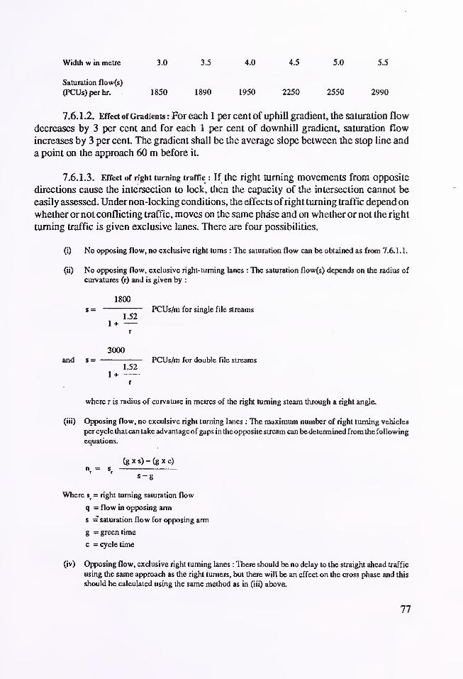
Width w in metre 3.0 3.5 4.0 4.5 5.0 5.5
Saturation flow(s)
(PCUs)perhr. 1850 1890 1950 2250 2550 2990
7.6. 1.2. Effect ofGradients : For each 1 per cent of uphill gradient, the saturation flow
decreases by 3 per cent and for each 1 per cent of downhill gradient, saturation flow
increases by 3 per cent. The gradient shall be the average slope between the stop line and
a point on the approach 60 m before it.
7.6.1.3. Effect of right turning traffic : If the right turning movements from opposite
directions cause the intersection to lock, then the capacity of the intersection cannot be
easily assessed. Under non-locking conditions, the effects ofright turning traffic depend on
whether or not conflicting traffic, moves on the same phase and on whether or not the right
turning traffic is given exclusive lanes. There are four possibilities.
(i) No opposing flow, no exclusive right turns : The saturation flow can be obtained as from 7.6.1.1.
(ii) No opposing flow, exclusive right-turning lanes : The saturation flow(s) depends on the radius of
curvatures (r) and is given by :
1800
1 +
s = PCUs/m for single file streams1.52
r
3000
and s = PCUs/m for double file streams1.52
1+r
where r is radius of curvature in metres of the right turning steam through a right angle.
(iii) Opposing flow, no exculsive right turning lanes : The maximum number of right turning vehicles
per cycle that can take advantage of gaps in the opposite stream can be determined from the following
equations.
(gxs)-(gxc)
s-g
Where sr= right turning saturation flow
q = flow in opposing arm
s = saturation flow for opposing arm
g — green time
c = cycle time
(iv) Opposing flow, exclusive right turning lanes : There should be no delay to the straight ahead traffic
using the same approach as the right turners, but there will be an effect on the cross phase and this
should be calculated using the same method as in (iii) above.
77
7.6.1.4., Effect of mixed traffic condition : The saturation flow gets reduced due to
presence of slow moving vehicles in the stream as the turning vehicles shall have to find
the suitable gap thereby affecting the average delay in the cycle.
7.6.2. Lost time : It is the time during which no flow takes place. It may be
(i) The total lost time per cycle (L)—The sum of lost time in each phase and this period when all signals
show red or red-amber. It can be expressed by,
L = nl + R
Where n = number of phases
1 = average lost time per phase (excluding any all red periods or sequent ambers)
R = all red period time during each cycle where all signals display red or red with amber.
(ii) the lost time for a single phase (1)—The amount of time in a cycle which is effectively lost to traffic
movement in phase because of starting delays and the falling of the discharge rate during amber
period. No flow takes place in lost time as would be seen in Fig. 7.6.
For the average signals cycle the lost time caused by starting delays and reduced
flow during the amber period amounts to about 2 seconds per phase.
7.6.3. Cycle time : The total time period required for one complete sequence of
signal indications is the cycle time. The cycle time with minimum delay could be
represented by.
Co = (1 .5L + 5)/( 1 - Y) seconds
where L = total lost time per cycle in seconds, generally taken as the sum of total amber and all red
clearance per cycle in seconds. Y = y, + y2+ ... ym
where y 5, y^
... ym are the maximum ratios of flow to saturation
flow for the phases 1, 2 ...n i.e. y = q/s for a given phase.
The minimum cycle length recommended is preferably 120 seconds being the
maximum acceptable delay for drivers of vehicles and pedestrians.
7.6.4. Green times : The effective green time (g) is the sum of green period and the
amber period (G) less the lost time (L) for a particular phase i.e. g = (G - L) seconds. The
ratio of effective green times should be equal to the ratio of by values.
ji_ = Jj_
where gj and g2are the effective green times of phase 1 and 2 respectively, yj and y2 are
maximum ofy values of phases 1 and 2 respectively. This rule can be extended to 3 or more
phase operations. The effective green time for a two phase intersection can be determined
from the expression
:
78

g,=—(Co - L) and g2= — (Co - L)
7.7. Control Measures
7.7.1. Channelisation : Channelisation involves the use of islands at intersections to
guide and protect the traffic. It provides reference points within the intersection which
enable drivers to better predict the path and speed of other drivers. They increase the
driver's ability' to avoid accidents and congestion. Channelised Islands should be at least
4.7m2 and preferably 7.1m2 in area, not less than 2.4 m and preferably 3.6 m on any side
after rounding of corners if triangular and at least 1.2 m and preferably 3.6 m if elongated.
7.7.2. Carriageway Markings : Carriageway markings and direction signs should be
located sufficiently in advance of the intersection to enable drivers to select and follow the
lane and path they should take through the intersection, Markings at intersections can be
a combination of centre lines, turn markings, lane markings, stop lines, route direction
arrows, pedestrian crossings etc. (Fig. 7.7)
LANE LINES 2.5-5.0 mWIDE CROSSING
-3 ,INDICATES SECONDARYSIGNALS
2nd PRIMARY^SIGNALS
D TYPEDETECTORLAYOUT
OETECTORS IN
APPROACH ASSH0WN-
Fig. 7.7. Signalised Intersection Layout and Carriageway Markings
79

7.8. Other Aspects
* 7.8.1. Visibility : The safety of traffic can be ensured only if the visibility is full and
unimpeded along both roads. Any obstruction should be clear of the minimum visibility
triangle for a height of 1.2 m above the roadway.
The intersection should be planned and located to provide as much sight distance as
possible. In achieving a safe highway design, there should be sufficient sight distance for
the driver on the minor highway to cross the major highway without requiring the
approaching traffic to reduce speed.
7.8.2. Installation of signals : The installation of signals and other technical aspects of
road traffic signals are discussed in detail in section II ofIRC : 93-1985 and may be referred.
A typical layout is shown in Fig. 7.8.
PREFERRED MINIMUM 1-5 mIF NO REFUGE PROVIDED WITHNARROW PAVEMENTS MAY NEEDTO BE REDUCED UPTO 0.6m.
SECOND PRIMARY SIGNAL
(WHERE THERE ARE TWOOR MORE LANES OFAPPROACH I NG TRAFFIC )
STOP LINE
1.5m MINIMUM30m RECOMMENDED
-*> PRIMARY SIGNAL
£ SECONDARY SIGNAL
2 5 -5 0 m WIDE PEDESTRIANCROSSING* 1-2 m WIDE REFUGE
PEDESTRIAN CROSSINGSTUDS
Fig. 7.8. Typical Layout of Traffic Signal Installations
80
8. SPECIAL CONSIDERATIONS IN URBAN AREAS
8.1. Control of Access
This aspect is discussed in detail in IRC : 62- 1 976 "Guidelines for Control ofAccess
on Highways". To ensure safe and efficient circulation of traffic, which serves the various
land uses adequately and ensures logical community development, the network ofroads in
an urban area has to be divided into different sub-systems each serving a particular function
or a purpose. The principal factors to be considered in designating roads into different
categories are the travel desire lines, access needs of adjacent properties, network pattern
and land use. For the purpose of these guidelines, urban highways/streets are considered to
be divided into the following types :
Arterial highways/streets,
Sub-arterial streets,
Collector streets; and
Local streets.
8.2. Spacing of Intersections
Although standards for the location of access points depend largely on the needs of
an area, the following guidelines which are indicative of good practice, may be followed
as far as possible.
8.2. 1. Spacing between intersections should have regard to the relevant geometric
design and traffic requirements, such as the type of traffic, length of right-turn or speed
change lanes etc.
As a rough guide, the suggested minimum spacing along various types of roads is
given below :
(i) Arterial highways/streets 500 metre
(ii) Sub-arterial streets 300 metre
(iii) Collector streets 150 metre
(iv) Local streets Free access
Where necessary, a greater distance than given above should be adopted, as for
example between junctions with linked traffic signals.
8.2.2. On arterial streets signals should preferably be linked to have a progressive
system, premitting continuous movement of vehicles at a planned speed of travel. As far
as possible, all such intersections should have approximately the same spacing.
(0
(ii)
(iii)
(iv)
81

8.2.3. Apart from regular intersections, limited number of access points with
intervening streets may be permitted at a spacing closer than mentioned in para 8.2.1
provided only left turns to and from the main street are permitted.
8.2.4. The location and spacing of all major points of access including accesses to
bus terminals, railway stations, parking areas etc. should be carefully planned so as to
ensure safety and freedom from congestion. Bus bays should not be located too close to
intersections. It is desirable that they are located 75m from the intersection on either side,
preferably on farther side of the intersection.
8.2.5. On arterials, direct access to residential plots is not to be permitted. Drive-
ways may, however, be permitted on a restricted basis for commercial and industrial
complexes and other public locations when these are major generators of traffic. Right turn
from these driveways should not be permitted unless the crossing fulfills the spacing
criteria given in para 8.2.1. Moreover, adequate road geometries should be provided to
enable safe operation of vehicles.
8.2.6. On sub-artenals, direct access to residential property should be granted only
where alternative access cannot be provided at a reasonable cost. Direct access to
commercial and industrial properties may be allowed.
8.2.7. On collector streets, access to abutting properties may be allowed to a limited
extent keeping in view the safety of traffic.
8.2.8. On local streets, which will have nc through traffic, access to abutting prop-
erties can be freely given.
8.3. Pedestrians at Junction
Pedestrian Crossings (e.g. at grade crossings, subways) should be designed at
intersection in accordance with the "Guidelines on Pedestrian Facilities" (IRC : 103-1988).
8.4. Cycle Tracks
8.4. 1 . It is desirable to segregate cycle traffic at intersections also since intersections
are dangerous, accident-prone locations. This could be achieved by a suitable system of
multi-phase signalisation.
8.4.2. Where cycle tracks are not segregated, suitable safety measures at intersec-
tions should be adopted, such as provision of separate lanes for cycle traffic, provision of
cycle boxes ahead of stop line, and provision of turning cycle paths in conjunction with
signalisation. These methods are shown in Fig. 8.1. Cyclist crossing must always be
marked in accordance with IRC : 35-1970.
82

83
8.4.3. At signalised intersections, a separate lane for cycie traffic alongwith a
reservoir space between pedestrians crossing zone and stop line for motorized vehicles
provides an efficient regulation. Fig. 8.2 shows the details of such layout. A separate cycle
track ofminimum 1.2 m width should be provided in the approaches of intersection. There
would be two stop lines, one for the motor vehicles and other for cyclists such that the
cyclists can wait in the reservoir space, for signal to turn green. The signs to be provided
and their locations as indicated in Fig. 8.2 are self explanatory.
8.5. Lighting & Sign Posting
The adequate lighting of intersections especially with channelising island is essen-
tial in urban areas. Lighting should be so done as to make the entire island and intersecting
area visible even in bad weather. The aspect of lighting is discussed in more detail in
Chapter 9.
The safety of intersection also depends on adequate carriageway markings, traffic
signs and delineators. These should be provided in accordance with IRC : 35-1970, IRC :
67-1977 and IRC: 79-1981.
9. LIGHTING, DRAINAGE, UTILITIES ANDLANDSCAPING OF INTERSECTION
9.1. Lighting at Intersections
Lighting affects the safety of highways and street intersections and the ease and
comfort of traffic operations. Statistics indicate that the evening accident rate is higher than
that during day-light hours. This fact, to a large degree, may be attributed to impaired
visibility. In urban and suburban areas where there are concentrations of pedestrians and
roadside and intersectional interference, fixed source lighting tends to reduce accidents.
9.1.1. Whether or not rural intersections at grade should be lighted depends on the
layout and the traffic volumes involved. Intersections that normally do not require
channelization are frequently left unlighted. On the other hand, intersections with substan-
tial channelisation, particularly multi-road layouts and those designed on a broad scale,
often are lighted. It is especially desirable to illuminate large-scale channelized intersec-
tions. There is need to obtain a reduction in the speed of vehicles approaching some
intersections. The indication of this need should be definite and visible at a distance from
the intersection that is beyond the range of headlights. Illumination of the intersection with
fixed-source lighting accomplishes this. The planned location of intersection luminairs
supports poles should be designed to present the least possible hazard to out-of control
vehicles. The breakaway support base should not be used within the limits of an at-grade
intersection, particularly in densely developed areas with adjacent sidewalks.
84

Fig. 8.2. Cyclists Crossing at Signalised Intersection
85

9.1.2. To minimize the affect of glare and to provide the most economic lighting
installation luminaries are mounted at heights of at least 9 m. Lighting uniformity is
improved with higher mounting heights, and in most cases mounting heights of 10 m to 15
m are usually preferable. High mast lighting, special luminaries on masts of 80m or morein height, is used to light large highway areas such as inter-changes. This lighting furnishes
a uniform light distribution over the whole area and may provide alignment guidance.
However, it also has a disadvantage in that the visual impact from spurious light is increased
to the surrounding community.
Lighting standards (poles) should be placed outside the clear zones whenever
practical. Where poles are located within the clear zone regardless of distances from the
travelled way, they should be designed to have the suitable impact attenuation features;
normally a breakaway design is used.
On a divided highway the street lighting standards may be either in the median or on
the left. Where lighting standards are located on the left, the light source is closer to the
more heavily used traffic lanes. However, with median installation, the cost is generally
lower and illumination is greater on the high-speed lanes. On median installations, dual-
mast arms should be used, for which 12m or 15m mounting heights are favoured. These
should be protected with suitable longitudinal barrier. On narrrow medians, it is usually
preferable to place the lighting standards so that they are integral with the median barrier.
Where highway lighting is being considered for future installation considerable
savings can be effected through design and installation of necessary conduits under
pavements and kerbs as part of initial construction.
9.2. Utilities
All highways and street intersections, whether upgraded within the existing right-of-
way or entirely on new right-of-way, generally entail adjustment of utility facilities.
Although utilities generally have little effect on the geometric design, full consideration
should be given to measures, reflecting sound engineering principles and economic factors,
necessary to preserve and protect the integrity and visual quality of the highway or street,
its maintenance efficiency and the safety of traffic. Depending on the location of a project,
involved utilities could include (1) sanitary sewers; (2) water supply lines; (3) oil, gas, and
petroleum products pipelines; (4) overhead and underground power and communication
lines; and (5) drainage and irrigation lines. IRC : 98-1988 "Guidelines on Accommodation
of Underground Utility Services Along and Across Roads in Urban Areas" provides
guidelines in this regard.
9.3. Drainage
9.3.1. Highway drainage facilities provide for carrying water across the right-of-
way and for removal of storm water from the road itself. These facilities include bridges,
culverts, channels, kerbs, gutters and various types of drains. Hydraulic capacities and
locations of such structures should be designed to secure as low a degree of risk of traffic
86
interruption by flooding as is consistent with the importance of the road, the design traffic
service requirements, and available funds.
9.3.2. Drainage inlets should be so designed and located as to limit the spread of
water on traffic lanes to tolerable widths. Because grates may become blocked by trash
accumulation kerb openings or combination inlets with both grate and kerb openings are
advantageous for urban conditions. Grate inlets and depressions and kerb-opening inlets
should be located outside the through traffic lanes to minimise the shifting of vehicles
attempting to avoid riding over them. Inlet grates should also be designed to accommodatebicycles and pedestrian traffic where appropriate. Inlets should be located so that concen-
trated flow and heavy sheet flow will not cross traffic lanes. Where pavement surfaces are
warped, as at cross streets, surface water should be intercepted just before the change in
cross slope. Also, inlets .should be located just upgrade of pedestrian crossing.
9.4. Landscaping
Landscape development at intersection should be in keeping with the character of
the highway and its environment. However, requirements of clear sight distance must be
kept in mind. Programmes include the following general areas of improvement : (1)
Preservation of existing vegetation (2) Transplanting of existing vegetation where feasible
(3) Planting of new vegetation, (4) Selective clearing and thinning, and (5) Regeneration
of natural plant species and material.
The objectives in planting or the retention and preservation of natural growth on
roadsides are closely related. In essence, they are to provide (1) Vegetation that will be an-
aid to aesthetics and safety, (2) Vegetation that will aid in lowering construction and
maintenance costs, and (3) Vegetation that creates interest, usefulness, and beauty for the
pleasure and satisfaction of the travelling public.
Landscaping of urban intersections assumes additional importance in mitigating the
many nuisances associated with urban traffic. Landscaping can reduce this contribution to
urban plight. For more detailed guidelines, reference to the IRC Manual on "Landscaping
of Roads", Published in 1979 may be made.
9.5. Right of Way
The right ofway for the road and area required for an intersection depend largely on
the type of highway topography and overall standards of intersection development. Therequired sight line at the intersection and impact on property access occurring with the
provision of intersection would also have to be considered. While deciding upon the area
required to be acquired for the intersection, drainage aspect and future planning, in
particular the need for the upgradation of intersection to a grade separated facility as
dictated by traffic projections, shall also be considered. The area shall be kept free from en-
croachments to facilitate the implementation of future planning.
87

APPENDIX-I
LAYOUT OF CURVES AT THE INTERSECTION
For proper design of curves for intersections a full appreciation of the turning path of vehicle is essential.
Fig. I- 1 shows the swept path of semi-trailer negotiating a 90° turn at low speed. Figs. 1-2, 1-3, 1-4, 1-5 and 1-6 show
details of wheel path and body overhang path1
of large car, single unit truck, semi-trailer, and large truck-trailer
combination respectively. Tamplates of these paths made to appropriate scale should be used to check layout of
curves at intersections. Figs. 1-7 to I- 10 show typical layouts of curves for a 90° turn using different vehicles and
curves.
.SWEPTPATH
PATH OF OUTSI0TRACTOR TIRE
PATH OF INSIDETRAILER TIRE
VEHICLE VEHICLETRACTORlm>
TRAILERUD)
SWEPT PATHim;
CASE1 3.0 13.9 8. 43
CASE 2 5. 4 14.4. 6. 4
CASE 3 3.3 8.4 6. 78
TRACTOR DIMENSIONS REPRESENT WHEEL BASE LENGTH
WHILE TRAILER DIMENSIONS ARE OVERALL TRAILER LENGTH
88
Fig. 1-1. Swept Path WidtJi for Various Truck Vehicles—Low speed Offtracking in a 90° Intersection Turn

• -rr-PATH OF RlOWt-^^ / /
EL >VFRONT WHEEL
PATH OFOVERHANG
Fig. 1-2. Minimum Turning Path for Passenger Car Design Vehicle (P)
89

90
Fig. 1-3. Minimum Turning Path for Single unit Truck Design Vehicle (su)
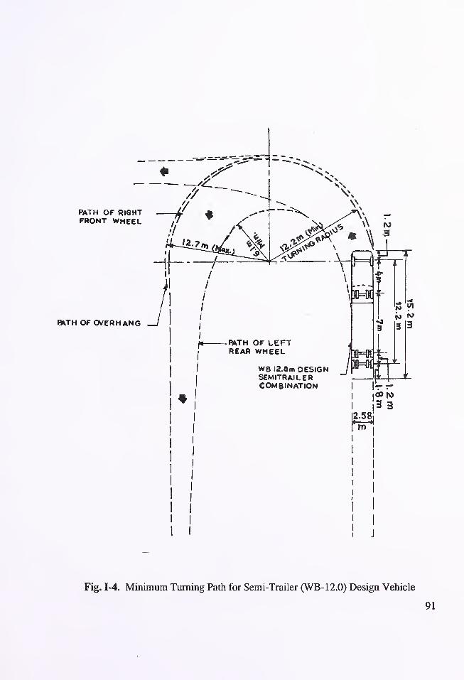
Fig. 1-4. Minimum Turning Path for Semi-Trailer (WB-12.0) Design Vehicle
91
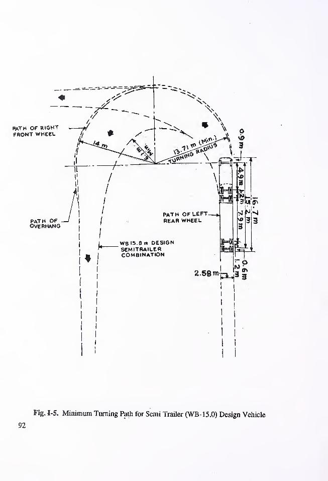
PATH OF RJGHTFRONT WHEEL
PATH OFOverhang
PATH OF LEFT-REAR WHEEL
WB 15.0 m OESIGNSEMITRAILERCOMBINATION
2.58 m
Fig. 1-5. Minimum Turning Path for Semi Trailer (WB-15.0) Design Vehicle
92

Fig. 1-6. Minimum Turning Path for Truck Trailer (WB-18.0) Design Vehicle
93

Fig. 1-7. Minimum Designs for Passenger Vehicles for 90° turn

SU DESIGNVEH1CUE PAT
^ 3-CENTERED COMPOUND CURVE\^36.6-l2.2'-36.6mRADII>OFFSET^6lm
Fig. 1-8. Minimum Designs for Single Unit Trucks and Buses for 90° Turn
95

3- CENTERED COMPOUND CURVE (ASYMETRICAU36.6-12 2 -61m RADII OFFSET 06im & 1.63 m
O
W8- 12.0 m SEMITRAILER COMBINATION
3- CENTERED COMPOUND CURVE 36. 6 ~ 12.2-36. 6mOFFSET 1.52m
96
Fig. 1-9. Minimum Designs for Semi-trailer Combinations (WB-12.0)
Design Vehicle Path for 90° Turn

WBH5 DESIGNVEHICLE PATH
'2> minimum Simple curvewith taper
•ft si m Radius offset 0.91w
W8-I3 DESIGNvehicle path
semitrailer combination
See"I!*?£iCOM P0UN0 CURVE « ASYMETRICAL
I
36.6-12 2 — 61 m RADII OFFSET O. 61 m ANO 3.05m
WB-13 DESIGNVEHICLE PATH
WB-)5 SEMITRAILER COMBINATION3- CENTERED COMPOUND CURVE54 9- 18 3- 34.9m OFFSET l.83n>
Fig. 1-10. Minimum Designs for Semi-trailer Combinations (WB-15)
Design Vehicle Path for 90° Turn

Appendix-I (Contd...)
The effect of angle of intersection on turning path and width occupied by vehicles with turning radii is
indicated in Table 1-1. This is useful in determining the desirable width of lane and corresponding radii of curve.
In Table 1-1 dj and d2are the widths occupied by the turning vehicles on the main street and on cross-street
respectively while negotiating turns through various angles. Both dimensions are measured from the left hand kerb
to the point of maximum turn.
The minimum radii of curves for various angles of intersection based on dimension in Table 4.5 are given
in Table 1-2.
2. Layout of three-Centered Compound Curve
Layout of 3-centered curves require calculations of offsets and co-ordinates and centre of curves. This can
be mathematically derived as below :
Let R, = First Radius xl
= First Offset
Rj = Middle Radius = Second Offset
Rj = Third Radius a = Angle of turn
Fig. I- 1 1 (a) shows the curve and its centres and Fig. I- 1 1 (b) is an enlarged plain of the required portion to
illustrate clearly.
Determination of the position of 'O' the centre of radius the middle radius; P
tQ is an arc drawn with
radius R,, Q R with radius R^ and R S with radius R^ having offset Xj at point Q and offset Xj at point R.
p,o, ii p2o
2or °2 d
IP.O.Q = IP02Q = Q I
...Fig. I- 11(a)
QE = C,P, = x, = First Offset ... Fig. I- 11(b)
C,P, = Rj - R, cos 0,
or x, = Rj - Rtcos 9j
or Cos 8, =Offset
Outer Radius
02D = 0
2C
2+ C
2D
= Rj Cos j + x,
0,D - *(«-^)«.
Therefore distance between A'02line AO.
= R2+ Xl— X
!
Rj or middle radius + offset fraction of offset which is equal to
offset multiplied by the ratio of middle radius to outer radius
98

Table 1-1. Urban Areas Cross-street width occupied by turning vehicle for
various angles of intersection and kerb radii
d2(m) for cases A and B where
R = 4.5m R = 6m R = 7.5 m R = 9m R = 12mDesign
Vehicle A B A B A B A B A B
30° SU 4.26 3.95 4.26 3.95 3.95 3.95 3.95 3.95 3.95 3.95
BUS 6.69 5.17 5.78 5.17 5.78 5.17 5.78 5.17 5.47 5.17
WB 40 4.26 4.26 4.26 4.26 4.26 4.26 4.26 4.26 4.26 4.26
WB 50 6.00 5.1 /ZT HA6.00 C 1 1
J. I /S f\f\6.00 .5.1 1
c no a on4.8 /
C AH5.4/
A On4.8 /
ou CT T < TOJ. /o A QH4.8 /
^ HQJ. /5 A 7C
4. / 5 A <4.
j
A C74.0 /A <
4.ZD A OC
BUS 8.55 6.38 7.9 6.0 7.23 6.0 6.99 5.78 6.69 5.47
WB 40 7.23 5.78 6.69 5.78 6.38 5.78 5.78 5.47 5.17 4.87
Wli JKJ O AO o.oy o.Z .Jo 8.55 Q GOo.oz /.o 5. /O D.oic AH5.4 /
yV CT Toil i on/.yo o.OU 0.99 jA 1 5. 10 4.0 / 5.1 /A <4.5 3.95 3.95
BUS 11.55 6.99 10.0 6.69 9.12 6.63 7.6 6.38 6.38 5.47
WB 40 9.43 6.69 8.2 6.38 6.99 6.38 5.78 5.47 5.17 4.87
WB 50 12.80 6.69 11.27 7.29 10.34 6.69 8.83 6.38 6.69 5.47
120° SU 10.34 6.69 8.2 5.78 6.38 5.47 5.17 4.78 3.95 3.95
BUS 13.98 8.55 12.2 7.6- 9.73 6.99 7.92 5.78 5.78 5.47
WB 40 12.23 6.99 8.83 6.69 7.23 6.69 5.78 5.47 5.17 4.87
WB 50 15.3 8.83 13.10 8.55 10.97 8.2 9.12 7.9 6.69 5.47
150° SU 12.2 7.6 9.75 6.30 6.69 5.79 5.17 4.87 3.65 3.65
BUS 14.59 8.55 12.2 7.6 9.75 6.99 6.69 5.47 5.17 4.87
WB40- 11:86 7.23 8.83 6.69 6.99 6.69 5.78 5.47 51.7 4.87
WB 50 16.11 9.43 14.0 8.55 10.97 8.2 8.55 7.92 6.69 5.47
Notes : P Design Vehicle Turns within 3.6 m width where R = 4.5 m No. parking Lanes on Either Street
d|s3.6m, 42 '* "enable = Both voriabht
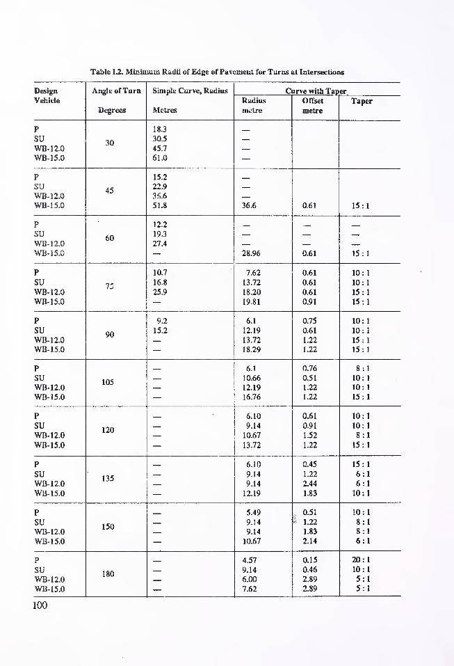
Table 12. Minimum Radii of Edge of Pavement for Turns at Intersections
Design
Vehicle
Angle of Turn
Degrees
Simple Curve, Radius
Metres
Curve with Taper
Radius
metre
Offset
metre
Taper
P
SUWB-12.0WB-15.0
30
18.3
30.5
45.7
61.0
PSUWB-12.0WB-15.0
45
15.2
22.9
35.6
51.8 36.6 0.61 15 : 1
PSUWB-12.0
WB-15.0
60
12.2
19.3
27.4
28.96 0.61 15: 1
P
SUWB-12.0
WB-15.0
1Z
10.7
16.8
25.9
7.62
13.72
18.20
19.81
0.61
0.61
0.61
0.91
10: 1
10: 1
15: 1
15: 1
PSUWB-12.0WB-15.0
90
9.2
15.2
6.1
12.19
13.72
18.29
0.75
0.61
1.22
1.22
10: 1
10: 1
15: 1
15: 1
P
SUWB-12.0
WB-15.0
105
6.1
10.66
12.19
16.76
0.76
0.51
1.22
1.22
8:110: 1
10: 1
15: 1
P
SUWB-12.0
WB-15.0
120
6.10
9.14
10.67
13.72
0.61
0.91
1.52
1.22
10: 1
10: 1
8:1
15: 1
P
SUWB-12.0
WB-15.0
PSUWB-12.0
WB-15.0
PSUWB-12.0
WB-15.0
135
150
180
6.10
9.14
9.14
12.19
5.49
9.14
9.14
10.67
4.57
9.14
6.00
7.62
0.45
1.22
2.44
1.83
0.51
1.22
1.83
2.14
0.15
0.46
2.89
2.89
15: 1
6:16:110: 1
10: 1
8:18:16:1
20: 1
10: 1
5:15:1
100

THREE CENTRED COMPOUND CURVE
D
Fig. 1-11. Three Centred Compound Curve

Appendix-I (Contd...)
Similarly distance between 0"B' rnd OB
X2
y 2=R, a- -r ) + x
2
= R + x - x^ 2 2
Procedure of Curve tracing :
Refer to Fig. 1-11
1. Draw line AO and OB at an angle a = angle'of turn.
2. Diaw line A O' and O ' B' parallel to A O and O B at distance Y and Y, respectively.
3. Knowing the Position of 02draw an arc of Radius R with centre at 0
?.
4. Draw line ClII A O at distance x
]
cutting the ^rc drawn wi'Ji centre 02at Q.
5 Extend Q 02upto O
tsuch ihat OjQ = R
t
and with Radius R(and centre Oj draw arc P
l Q touching AOat P, (Tangent).
6. Similarly draw the other curves RS.
P, Q R S is the required 3 centred curve with offset xta* Q and x
2at R.
Tables 1-3,1-4 and 1-5 give some typical values ofY ,YjandR^Rj and Rj for various angles of forms
and design of vehicles depending upon whether the compound curve is symmetrical or assymmetrical
with the help of these Tables, the 3-centred compound can be drawn.
102

Table l-J. 3 Centered Compound Curve (Symmetrical) Without Channelising Island
Vehicle
1
A tic Ip of
Turn
Radii
(Metres)
Offset
Centre ofMiddleq -?->/» if* »»i <kf r°i»c*? V 111 Lildl ca
W3- 15.0 45° 61.0 - 30.5-61.0 0.91 30.955
Wd - ID V oU Di U-ZZ V-01.U 1 ,UO
p 75° 30.5-7.6-30.5 0.61 8.0<o
su 36.6-13 7 36.6 0.61 14.082
WB 12.0 36.6-13.7-36.6 1.52 14.651
WB 15-0 45 7-15 2-45 7 1.83 16.421
P 90° 30.5-6 1-30.5 0.76 6.7C3
SU 36.6-12.2-36.6 0.61 12.607
W D - 1Z.U JO.O- i—.Z- JO.O l.JZ 1 J.Z1 J
WB - 15.0 54.9-18.3-54.9 i.83 19.520
P 105° 30.5-6.1-30.5 0.76 6.700
SU 30.5-10.7-30.5 0.91 11.291
WB - 12.0one i n fi nit"!30.5-10.0-30.7 1.52 1 1.687
P 120° 30.5-6.1-30.5 0.76 6.708
SU 30.5-9. 1 -30.5 0.91 9.738
WB - 12.0 36.6-9.1-36.6 1.83 10.475
WB - 15.0 54.9-12.2-;>4.9 2.59 1^.214
P 135° 30.5-6.1-30.5 045 6.460
SU 30.5-9. J -30.5 1.22 9.956
WB - '2.0 36.6-9.1-36.6 1.98 10.588
*V kJ 1J.U 48 ft 1 0 1 4ft ft Z. /
1
p 150c 20.9-5.9-20.0 0.76 6.445
SU 30.5-9.1-30.5 1.22 9.956
WB-12.0 30.5-9.1-30.3 1.83 10.384
WB - 15.0 48.8-10.7-48.8 2.13 12.363
P 180° 15.2-4.6-15.2 0.15 4.705
SU (UTurn) 30.5-9.1-30.5 1.37 10.061
WB - 12.0 30.5-6.1-39.6 2.90 8..420
WB - 15.0 39.6-7.6-39.6 2.90 9.943
103

Table 1-4. 3 Centred Compound Curve (Assymetrical) Without Channelising Island
Design Angle of Radii Offset Co-ordinates of centre
Vehicle Turn Metres metre of middle arc
WB-150 60° 61.0-0.22.9-83.8 0.61-1.83 23.281 24.230
WB-12.0 75° 36.6-13.7-61.0 0.61-1.98 14.082 15.235
WB-15.0 45.7-15.2-68.6 0.61-3.05 15.607 17.574
WB-12.0 90° 36.6-12.2-61.0 0.61-1.83 12.607 13.664
WB-15.0 36.6-12.2-61.0 0.61-3.05 12.607 14.640
WB-12.0 105° 30.5-10.7-61.0 0.61-2.44 11.096 12.712
WB-15.0 45.57-12.2-64.0 0.61-3.05 12.647 14.669
WB-12.0 120° 30.5-9.1-54.9 0.61-2.74 9.523 9.609
WB-15.0 45.7-10.7-67.1 0.61-3.66 11.167 13.776
WB-12.0 135° 30.5-7.6-54.9 0.91-3.05 8.283 10.228
WB-15.0 39.6-9.1-56.4 0.91-4.27 9.301 12.681
WB-12.0 150° 27.4-7.6-48.8 0.91-3.35 8.258 10.428
WB-15.0 36.6-9.1-54.9 0.91-4.27 9.784 12.662
WB-12.0 180° 25.9-6.1-45.7 1.83-3.96 7.499 9.531
WB-15.0 30.5-7.6-54.9 1.83-3.96 8.974 11.012
Table 1-5. 3 Centred Compound Curve (Symmetrical)-With Channelising Island
Angle of Radii Offset Co-ordinate of centre
Turn Metres Metres of middle arc (in metres)
SU 75° 45.7-22.9-45.7 1.52 23.658
WB-15.0 54.9-27.4-54.9 1.07 27.936
SU 90° 45.7-15.2-45.7 1.52 16.214
WB-15.0 54.9-19.6-54.9 1.03 20.262
SU 105° 30.5-10.7-30.5 1.52 11.687
WB-15.0 54.9-13.7-54.9 2.44 15.531
SU 120° 30.5-9.1-30.5 0.91 9.738
WB-15.0 54.2-12.2-54.2 2.59 14.207
SU 135° 30.5-9.1-30.5 1.22 9.956
WB-15.0 48.8-10.7-48.8 2.74 12.839
SU 150° 30.5-9.1-30.5 1.22 9.956
WB-15.0 48.8-10.7-48.8 2.13 12.363
04
APPENDIX -II
CAPACITY ASSESSMENT OF AT GRADE INTERSECTION(BASED ON U.K. PRACTICE)
1. Type of Movements & Capacity
1.1. The actual capacity of intersection depends on the type of vehicle manoeuvres, the distribution of
gaps in the traffic stream and the drivers judgement in selecting gaps through which to execute the desired
manoeuvre. There is only limited information available on the capacity of intersections in India, as such we have
to fall back on information available abroad for guidelines, till relevant studies are completed in the country. Fig.
II- 1 gives the types ofmovements that occur at unsignalised intersections and the subsequent section describes the
possible capacities for such movements.
(1) Merging : Fig. II - 1(a)
This movement may take place by means of an acceleration lane or simply by an entry curve.
An estimate of the maximum slip road flows for different main road flows for rural situations can be made
by use of curves in Fig. II - 2 which shows these flows for different carriageway widths. There curves adopted in
U.K. may not necessarily be applicable to all Indian traffic conditions. Where the expected slip road flows exceed
the maximum flows given in the Fig. II-2 it will be necessary to provide an additional lane to the main road.
The slip road capacities do not apply when there are other nearby road connections and their effect is to
increase or decrease the volume in the nearside lane according to their position and direction of flow. The effect is
most marked by ori-road connections upstream within 1 30 m and somewhat less at 150 m to 300 m distance.
For the effect of downstream off-road connections, reference should be made to weaving capacity
limitations.
Where no acceleration lane is provided, the capacity -of the slip road entry onto a dual two-lane road maybe assumed for design purposes to be 290 p.c.u's/hour less than with an acceleration lane, greater differences have
sometimes been experienced.
(2) Diverging Fig. II- 1(b)
The capacity of a slip road exit may be taken to be 1 ,200 p.c.u' s/hour provided the deceleration lane is well-
designed and sign-posting gives adequate warning well in advance of the junction. In the case of dual three orfour-
lane roads when the flow off the slip road approaches the capacity of one lane, it may be appropriate to reduce the
main carriageway by one lane beyond the slip road connection.
(3) Cutting Fig. II- 1 (c) & (d)
A cutting manoeuvre may be a simple right-turn cut of one stream traffic across the opposing stream, or
across a two-way stream of traffic. These movements take place in the naturally occurring gaps in the traffic streams
which are of suitable duration. The larger traffic gaps are utilised by several vehicles cutting at one time.
As in general, the flow of traffic on a road approximates to a random distribution, calculations can be madeof 'Capacity' which depends on the size of gaps required and the volume and speed of the traffic stream which must
be crossed. For conditions ofgood visibility the curves shown in Fig. II - 3 give the minor road flow which can cross
different major road flows either one or two-way for different sizes of traffic gaps. These are applicable to rural
intersections. For one-way flows, e.g. across one carriageway of a dual carriageway road it would be reasonable to
assume average minimum gaps of 4 - 6 seconds, and across the dual carriageway 6-8 seconds. As per a study on
its at grade-intersections for Indian mixed traffic conditions the critical gaps have been found to be of a similar
105

magnitude. For the higher design speeds, larger gaps should be used. These capacities need to a single, lane from
the minor road ; capacity can be increased by providing two lanes if these could be used effecting.
(4) Cutting and Merging : Fig. II- 1(e)
Unlike the simple cutting of two-way flows this manoeuvre requires traffic gaps of sufficient duration for
the turning vehicle to accelerate to a suitable speed to join the far traffic stream and traffic gaps of 8-12 seconds maybe needed ; Fig. II - 3 gives the appropriate volumes.
(5) Compound Cutting and Merging : Fig. II - 1(f)
This type of movements takes place at a simple 'T' intersection. The normal sequence is for the right turn
(Rj) into the minor road to precede the right turn (R^ from the minor road. Precise calculations are complex and for
most purposes it is reasonably accurate to add half of Rj to and the capacity can be calculated using the gap sizes
appropriate for cutting and merging even in Section (4) above.
(6) Reservoir Space : Fig. II- 1 (g)
Where vehicles wait for opportunities to cross traffic streams, queues of vehicles develop and these need
to be accommodated in suitable 'reservoir' spaces. The number of vehicle spaces needed varies due to the chance
arrival of the turning vehicles and also due to the distribution of gaps of sufficient duration for the crossing to be
made.
For roads with deceleration lanes in the central reserve it is not usually necessary to consider added length
to the deceleration lane to cater for the wide variation in the number of vehicle waiting to turn.
For some intersection designs, such as left/right staggered intersections, the storage area is limited. These
intersections should preferably be used up to the limit of capacity found by using 8 second gaps, and a storage space
should be allowed for 8 vehicles. For lighter flows a minimum of 4 vehicle spaces is recommended. A length of 6
m for each p.c.u. may be assumed.
(7) Weaving : Fig. II - 1 (h) and (i)
The term weaving is applied to the combined movement of merging and diverging. There are two distinct
types, namely (a) weaving at round abouts and (b) weaving aiong roads. In both cases there are normally othertraffic
streams which are non weaving, see Fig. II - 1(h) & II - l(i) which indicates weaving streams and non-weaving
streams.
1.2. In the case of roundabouts the capacity can be estimated from the capacity formula adopted in IRC:
65 - 1976.
2. Capacity of Intersections in Urban Conditions
2.1. An assessment of the intersection capacity in urban conditions can be made from the curves
developed for the conditions and given in Fig. II -4. These curves are applicable to both T-intersections and cross
roads. Staggered cross roads should be regarded as two T-intersections for direct cross roads the curves indicate the
traffic that can enter from the more heavily trafficked side road.
2.2. The curve A in Fig. II - 4 shows the maximum volume of side road traffic whichmay cross different
through flows on the main road based on the assumptions of a single lane side approach per visibility from the side
road and a minimum acceptable gap of 8 seconds. The poor visibility will imply that when visibility on the approach
road is restricted but is adequate for stop conditions.
2.3. Curve Bin Fig. II- 4 shows the increased capacity under conditions ofgood visibility thus permitting
vehicles from the side road to enter suitably in long gaps in platoons without each vehicle necessarily having to stop
at the major road is based on a minimum acceptable gap of 6 seconds.
106
3. Weaving along roads : Fig. ll-l(i)
The effect of weaving along roads on road capacity depends upon the spacing of interesections and volumes
of weaving traffic streams. To calculate the appropriate road width and spacing of intersections reference should
be made to Fig. II-l(i).
The number of lanes required for minimum weaving sections may be estimated from the formula given
below. To allow foi mixed traffic, mainly flows should be given in PCU's factors applicable to urban area.
W, + 3W, + F, +r
C
Where
N Number of lanes
larger weaving flow in PCUs/hr.
w2
= smaller weav ing flow in PCUs/hr.
F,&F2
= outer non-weaving stream in PCUs/hr.
C normal lane capacity of the major road.
For given total volumes of weaving traffic, the minimum length of weaving section can be read from the
diagram and the lane capacity for the minor weaving movement can be determined from right hand scale (Fig. II-
5).
The number of lanes required in the weaving section can be found by summing the total of the non-weaving
flow plus the. major weaving flow and dividing by 1 ,200 and adding to this the minor weaving flow divided by the
appropriate lane capacity for minor weaving movement. The latter can be obtained from Fig. II-5 given the weaving
length and total weaving volume, see example given in the diagram. Where the calculated width is less than 3 lanes
and one of the non-weaving flow exceeds 600 p.c.u.'s/hour, two additional lanes should be providsd for non-
weaving traffic.
4. Signal Controlled Movements (See Chapter 7 also)
In some instances particularly in semi-rural areas where signal control is applicable intersection may be
designed on channelising principles and signal control applied to simple traffic counts. In such instances capacity
checks could be made by taking the maximum flows per lane width (expressed in p.c.u's) for each phase and
summed for the two phases. This sum then can be < mpared with a practical capacity of 1 ,600p.c.u's/hour per traffic
lane, thus lane densities in two phases of 800/ NOO, 1,000/000, 1,200/400, etc. would be maxim^-ni practical
capacities according to the proportions in the two phases.
107
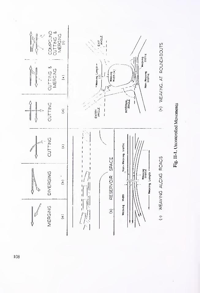
A
V
A
z
Vu
ZuLU
A
V
zh-
u
/V
f—Hu
ozocrUJ>a
zoaLU
2
U)
u<
/I
toI—
8til
<i
QZD
<6z
LU
a8a
zo<oz><LU
c
E>o
T3
Coo
5
WD
108

til
2D•J
O>Q<oa
ac
zbl
-I
<ac
ac
ac
zv,
mDOa
1200
IIOO
1000
900
800
700
600
500
400
300
200
100
Ko„Ski ^* 1
fefHi
1000 2000 3000 4000 5000 6000 7000
MAJOR ROAD VOLUME (IN ONE DIRECTION !
UPSTREAM OF ENTRY SLIP ROAD (PCU*S/HR) (RURAL)
Fig. II-2. Capacity of Merging Flows
109
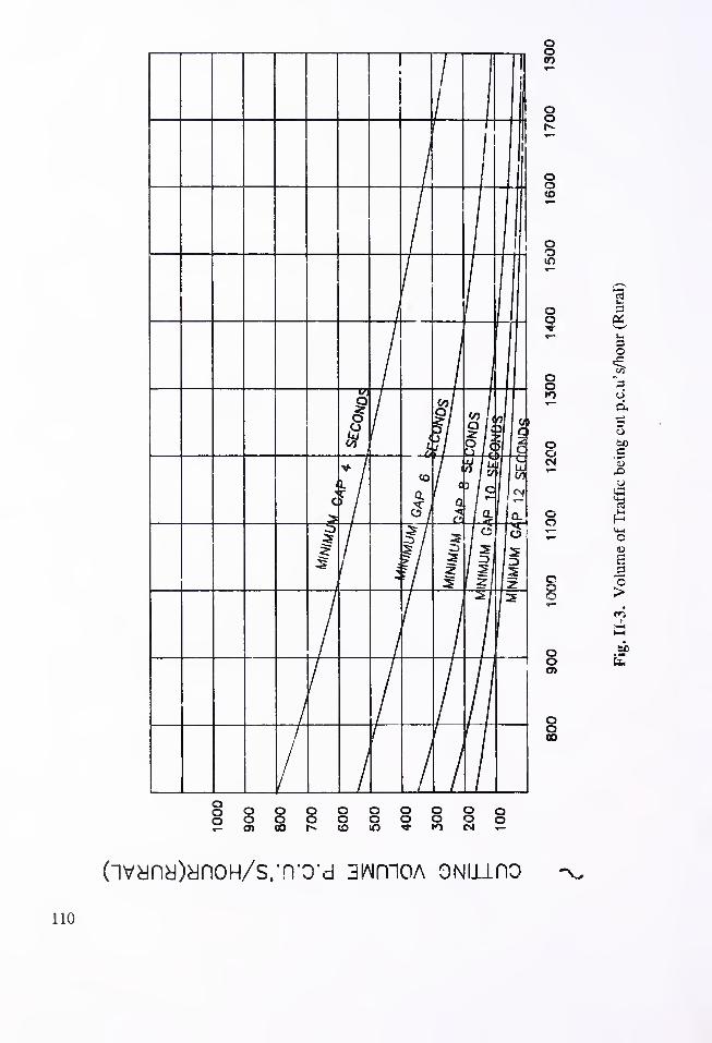
(ivana)anoH/s,,
n,
o,
d 3wmoA oniiido

exUJ
2 200
uu
I CURY£A !CPoor visibility I j ~-JI L I J '->n offrccchj J _p
<cr
,00-
600 TOO
OTV.E;{ WHEP.E PROVlStOfj IS UADE FOfi
SI0£ 1^0*0j
M^eyEms
BOO !00G !IOO 1200
MAIN ROAD TRAFFiC (TOTAL FOR BOTH DIRECTIONS, EXCLUSIVE OF TURING
TRAFFIC) - V PH
JFig. II-4. Capacity of uncontrolled Ti tersection
111

LENGTH OF WEAVING SECTfON ( METRES )
EXAMPLE LENGTH BETWEEN JUNCTIONS -I600MNON WEAVING TRAFFIC — 1700 pcu's/hr,
MAJOR WEAVING TRAFFIC- '450 pcu>s/hr.
MINOR WEAVING TRAFFIC- 550 pcu's/hr.
FROM DIAGRAM FOR TOTAL WEAVING VOLUME OF 2000pcu»s/hr. AN 0 WEAVING LENGTH 1600 m. CAPACITYPER LANE FOR MINOR WEAVING MOVEMENT- 880 pcu's/hr
PER LANE .
.'. NUMBER OF LANES IN WEAVING SECTION IS-
1700+1450 . 550T — 3 d -J
1200 880
i.e 4 TRAFFIC LANES
NOTE : PCU'S GIVEN ABOVE ARE RURAL STANDARDBASED ON MATERIALTHE COPYRIGHT OF THEHIGHWAY RESEARCH BOARD, U.S.A.
Fig. II-5. Capacity of Long Weaving Section Operating through Speed 70 km/hr.
112

APPENDIX -III
CAPACITY OF UNSIGNALISED INTERSECION
1.1. Introduction
The analysis of unsignalized intersections is generally applied to existing locations either to evaluate
existing operational conditions under present demands,or to estimate the impacts of anticipated new demands. The
methodology is specifically structured to yield a level of service (LOS) and an estimate of reserve capacity for an
existing case. Thus, operational analysis is the mode in which it is used. Design applications are treated as trial-and-
error computations based on anticipated improvements to an existing intersection or on the design of a newintersection for the projected traffic.
The method generally assumes that major street traffic is not affected by minor street flows. The
methodology al so adjusts for the additional impedence ofminor street flows on each other and accounts for the share
use of lanes by two or three minor street movements.
1.2. Field Data Requirements
Computations require following types of data inputs to the methodology :
(i) Volume by type of movement for the design hour
(ii) Vehicle classification for the design hour
(iii) Peak hour factor (if peak flow rates are being used as the basis for analysis)
(iv) Prevailing (average running) speed of traffic on the major street
(v) Number of lanes on the major street
(vi) Number of lanes on the minor street approaches
(vii) Other geometric features i.e. channelization, angle of intersection, sight distance, comer radii,
acceleration lanes, etc.
(viii) Type of control on the minor approaches.
Because the methodology herein results in a qualitative evaluation of delay, it is also recommended, if
possible, that some delay data be collected with the above information. This will allow for a better quantification
and description of existing operating conditions at the location under study. It would also allow for a more precise
comparison with a signalized intersection analysis for which delay estimates are generated.
1.3. Sequence of Computations
As the methodology is based on a prioritized use of gaps by vehicles at an unsignalized intersection, it is
imponant that computations be made in a precise order. The computational sequence is the same as the priority of
gap use, and movements are considered in the order i .e. Left turns from the minor street. Right turns from the major
street, through movements from the minor street and Right turns from the minor street.
1.4. Analysis of Four-Leg Intersections
The following steps describe the procedure of computations :
1.4.1. Volume summary and adjustment : The first page of the worksheet [Fig. Ill (5a)] consists of sum-
marization and adjustment of demand volumes. Basic geometric data are also summarized on this page.
(i) Hourly volumes are summarized on the top portion of the form on the diagram provided. A 'north'
indication should be inserted to ensure proper orientation of the intersection and of the demandvolume. V, to V
6denote movements and on major street and V
7to V denote movements on minor
street.
(ii) The number of lanes on each approach should be indicated.
113
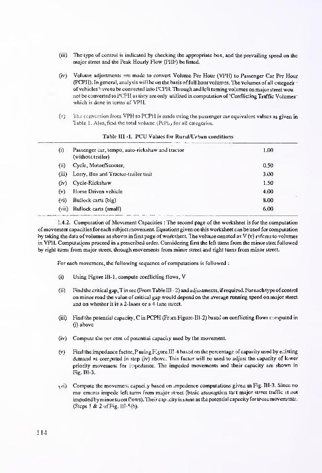
(iii) The type of control is indicated by checking the appropriate box, and the prevailing speed on the
major street and the Peak Hourly Flow (PHF) be listed.
(iv) Volume adjustments are made to convert Volume Per Hour (VPH) to Passenger Car Per Hour(PCPH). In general, analysis will be on the basis of full hour volumes. The volumes of all categorif 1
of vehicles h ave to be converted into PCPH. Through and left turning volumes on major streetwounot be converted to PCPH as they are only utilized in computation of 'Conflicting Traffic Volumeswhich is done in terms of VPH.
(v) The conversion from VPH to PCPH is made using the passenger car equivalent values as given in
Table 1. Also, find the total volume (PcPh) for all categories.
Table III -1. PCU Values for Rural/Urban conditions
(i) Passenger car, tempo, auto-rickshaw and tractor 1.00
(without trailer)
(ii) Cycle, Motor/Scooter, 0.50
(iii) Lorry, Bus and Tractor-trailer unit 3.00
(iv) Cycle-Rickshaw 1.50
(v) Horse Driven vehicle 4.00
(vi) Bullock carts (big) 8.00
(vii) Bullock carts (small) 6.00
1.4.2. Computation of Movement Capacities : The second page of the worksheet is for the computation
of movement capacities for each subject movement. Equations given on this worksheet can be used for computation
by taking the data of volumes as shown in first page of worksheet. 1he volume denoted as V (v) referes to volumes
in VPH. Computations proceed in a prescribed order. Considering first the left turns from the minor stret followed
by right turns from major street, through movements from minor street and right turns from minor street.
For each movement, the following sequence of computations is followed :
(i) Using Figure III- 1 . compute conflicting flows, V
(ii) Find the critical gap, T in sec (From Table III 2) and adjustments, if required. Foreach type ofcontrol
on minor road the value of critical gap would depend on the average running speed on major street
and on whether it is a 2-lanes or a 4-lane street.
(iii) Find the potential capacity, C in PCPH (From Figure-III-2) based on conflicting flows c jmputed in
(i) above
(iv) Compute the per cent of potential capacity used by the movement.
(v) Find the impedance factor, P using Figure III-4 based on the percentage of capacity used by casting
demand ?s computed in step (iv) above. This factor will be used to adjust the capacity of lower
priority movement for impedance. The impeded movements and their capacity are shown in
Fig. III-3.
(vi) Compute the moveme.ii capaci.y based on .mpedence computations given in Fig. III-3. Since no
mo emcnts impede left turns from major street (basic assumption that major street traffic is not
impeded by minor street flows). Their cap ;city is same as the potential capacity for thesemovements
.
(Steps ! &2of Fig. IK-5(b).
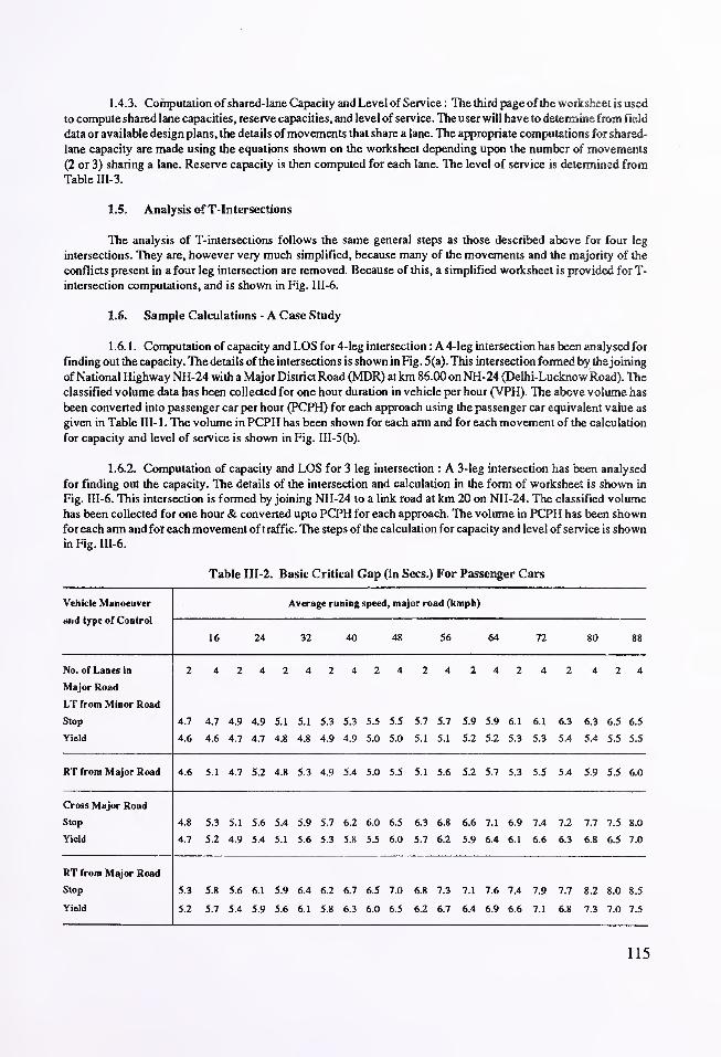
1.4.3. Computation of shared-lane Capacity and Level of Service : The third page ofthe worksheet is used
to compute shared lane capacities, reserve capacities, and level of service. The user will have to determine from field
data or available design plans, the details ofmovements that share a lane. The appropriate computations for shared-
lane capacity are made using the equations shown on the worksheet depending upon the number of movements
(2 or 3) sharing a lane. Reserve capacity is then computed for each lane. The level of service is determined from
Table III-3.
1.5. Analysis of T-Intersections
The analysis of T-intersections follows the same general steps as those described above for four leg
intersections. They are, however very much simplified, because many of the movements and the majority of the
conflicts present in a four leg intersection are removed. Because of this, a simplified worksheet is provided for T-
intersection computations, and is shown in Fig. III-6.
1.6. Sample Calculations - A Case Study
1.6.1. Computation of capacity and LOS for 4-leg intersection : A 4-leg intersection has been analysed for
finding out the capacity. The details of the intersections is shown in Fig. 5(a). This intersection formed by thejoining
of National Highway NH-24 with a Major District Road (MDR) at km 86.00 on NH-24 (Delhi-Lucknow Road). The
classified volume data has been collected for one hour duration in vehicle per hour (VPH). The above volume has
been converted into passenger car per hour (PCPH) for each approach using the passenger car equivalent value as
given in Table III- 1 . The volume in PCPH has been shown for each arm and for each movement of the calculation
for capacity and level of service is shown in Fig. III-5(b).
1.6.2. Computation of capacity and LOS for 3 leg intersection : A 3-!eg intersection has been analysed
for finding out the capacity. The details of the intersection and calculation in the form of worksheet is shown in
Fig. III-6. This intersection is formed by joining NH-24 to a link road at km 20 on NH-24. The classified volume
has been collected for one hour & converted upto PCPH for each approach. The volume in PCPH has been shown
for each arm and for each movement of traffic. The steps of the calculation for capacity and level of service is shown
in Fig. III-6.
Table III-2. Basic Critical Gap (in Sees.) For Passenger Cars
Vehicle Manoeuver
and type of Control
Average runing speed, major road (kmph)
16 24 32 40 48 56 64 72 80 88
No. of Lanes in
Major Road
LT from Minor Road
Stop
Yield
2 424242424 24 2424 2 424
4.7 4.7 4.9 4.9 5.1 5.1 5.3 5.3 5.5 5.5 5.7 5.7 5.9 5.9 6.1 6.1 6.3 6.3 6.5 6.5
4.6 4.6 4.7 4.7 4.8 4.8 4.9 4.9 5.0 5.0 5.1 5.1 5.2 5.2 5.3 5.3 5.4 5.4 5.5 5.5
RT from Major Road 4.6 5.1 4.7 5.2 4.8 5.3 4.9 5.4 5.0 5.5 5.1 5.6 5.2 5.7 5.3 5.5 5.4 5.9 5.5 6.0
Cross Major Road
Stop
Yield
4.8 5.3 5.1 5.6 5.4 5.9 5.7 6.2 6.0 6.5 6.3 6.8 6.6 7.1 6.9 7.4 7.2 7.7 7.5 8.0
4.7 5.2 4.9 5.4 5.1 5.6 5.3 5.8 5.5 6.0 5.7 6.2 5.9 6.4 6.1 6.6 6.3 6.8 6.5 7.0
RT from Major Road
Stop
Yield
5.3 5.8 5.6 6.1 5.9 6.4 6.2 6.7 6.5 7.0 6.8 7.3 7.1 7.6 7.4 7.9 7.7 8.2 8.0 8.5
5.2 5.7 5.4 5.9 5.6 6.1 5.8 6.3 6.0 6.5 6.2 6.7 6.4 6.9 6.6 7.1 6.8 7.3 7.0 7.5
115

Adjustments and Modifications to Critical Gap, Sec
fnn#fl itloncvkUiiu iiivua Rpmark<i
(i) LT from Minor Street -0.5 , - Maximum total decrease in
(Curb radius > 15m, critical gap =1.0 sec.
turn angle < 60°) Max. Critical gap = 8.5 sec
(ii) LT from Minor Street 1 r\- IAJ Interpolation can be made for
(Acceleration lane values of average running
nrAviiiPn ll/I \J V lUvUJ speed between 48 and 88 kmph.
(iii) All Movement -0.5 * The adjustment is made for the specific movement
(Population > 2.5 lacs) if impacted by restricted sight distance
(iv) Restricted Sight + 1.0
Distance
TABLE III-3 :; Level-of-Service Criteria for Unsignalized Intersections
Level of Service Expected Delay to Minor
(pcph) (LOS) Street Traffic
>400 A Little or no delay.
399 - 300 B Short traffic delays
299 - 200 C Average traffic delays
199-100 D Long traffic delays
99-0 E Very long traffic delays
F Stops-and-starts
116
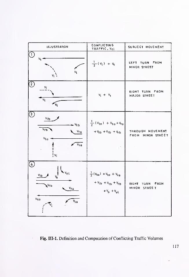
ILLUSTRATIONCONFLICTIN GTRAFFIC , Vci
SUBJECT MOVEMENT
©v*-
V;\
-f <vL
) + vt
LEFT TURN FROMMINOR STREET
WVi
\
Vt
vt+ v
t
RIGHT TURN FROMMAJOR STREET
©^vtb
V*o
| ? Vi a
1
1
!vi
y(v la )+vta + vra
+ vlb + vtb +vrb THROUGH MOVEMENTFROM MINOR STREET
(4)
_^>_>
>
— ( \l. ) 4- Vi -4- V
+ v ib +vtb + vrb RIGHT TURN FROMMINOR STREET
Fig. III-l. Definition and Computation of Conflicting Traffic Volumes
117

118

© R T FROM MINOR-STREET AT A T - INTERSECTION
MINOR
Cm = C P x Pl1 * p12 x Po
x Pol
Fig. III-3. Illustration of Impedance Computations

120

Name : KM 86/000 (NH/MDR)
Hourly Volume : in vph
Laclion : Garhmukteshwar
n. mStop \~s\
yield| [
(2) <-
Bulandshahar
(3)
NH-24T136
Ghaziabad
4 10
v, v2
v,
2
24
Nil
N
MDR(4)—
»
Meerut
Minor Road
t_L
NIL1222
r
24
22
144
70
Date of Counts
Time Periods
Average Running Speed
32 kmph
Major road
iMoradabad
(1)
Volume Adjustment
1 2 3 4 5 6 7 8 9 10 11 12 Movement No.
4 136 10 70 222 Nil 24 22 144 Nil 24 2 Volume (vph)
4 163 12 85 265 Nil 30 27 173 Nil 30 2 Volume (pcph)
Volume in pcph
1 f 1
4 NA NA
v. v, v,
(2)
2
30
NIL
J (4)
^ T
j_ 1NA NA
i
(1)
Fig. Ill 5(a). Worksheet for Four Leg Intersections
121
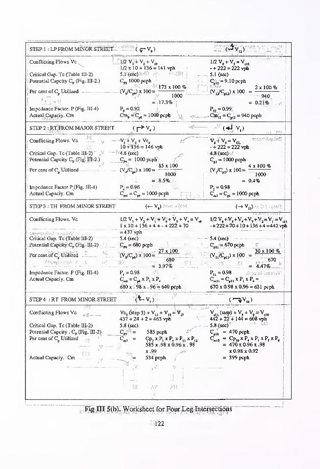
STEP 1 : LP FROM MINOR STREET < ^- V,
)
Conflicting Flows Vc l^Vj + Vj + V^, 1/2 Vf+ V, = V
cI2
1/2 x 10 + 136 = 141 vph|
- + 222=222vphI Critical Gap. Tc (Table m-2) 5l^^dD 5.1 (sec)
Potential Capcity C, (Fig. m-2.) 1 000 pcph Cpl2
= 9. 1 0 pcph
173 x 100 % 2 x 100 %Per cent of C Utilized (VJCJ x 100= (VJC.,-) x 100 =
p * • 1000tf pU
940
(I 1= H =517.3% s = 0.21%
Impedance Factor. P (Fig. m-4) P9= 0.92 P,
2= 0.99
Actual Capaciy. Cm Cmj = C# = 1000 pcph Cmj2= C
pl2= 940 pcph
STEP 2 : RT FROM MAJOR STREET ( r> V. ) nV ( <J V,
)
-—..a
' m . -* <r>
Conflicting Flows. Vc - -V,+ V2+ Vc
4V
6+ V, = Va
10 +136 = 146 vph - + 222 = 222 vph
Critical Gap. Tc (Table m-2) 4.8 (sec) 4.8 (sec)
Potential Capcity Cp (FigTffl-2.) Cp4= 1000 pcph C
pl= 1000 pcph
85x 100 4x100%Per cent of C Utilized _ (V./C .) x 100 = — (V,/C ,) x 100 =
p:
1000 ;
1 pl1000
= 8.5% = 0.4%
Impedance Factor P (Fig. IH.-4) P4
; = 0.96 Pt= 0.98
Actual Capaciy. Cm Cro4= C
p4= 1000 pcph Cnl
= CpI= 1 000 pcph
STEP 3 :TH FROM MINOR STREET (<- V,) [«M (-» V„)
Conflicting Flows. Vc 1/2 V3+ V
2+ V, + V- + V, + V
4= 1/2 V
s+V
s+V.
t+V,+V
2=V
l=V
C„1 x 10 + 136 + 4 + - + 222 + 70 - + 222 + 70+ 10 + 136 + 4 =442 vph
3noinJ?iJjb/, tmuldV =437 vph
Critical Gap. Tc (Table m-2) 5.4 (sec) 5.4 (sec)
Potential Capcity C, (Fig. ffl-2) Cre= 680 pcph CpU = 670 pcph
a-. ... ,jr_v c 27 x 100 30 x 100 %Per cent of C„ Utilized (VJCJ x 100= —^
^- (V../C...) x 100 = —I
p 1,7 "* 68011 pU 670
= 3.97% = 4.47% J-!Impedance Factor. P (Fig. m-4) P
}= 0.98 P„ = 0.98
Actual Capaciy. Cm Cm8= C^ x P, x P
4C.„ = C
pllx P, x P
4=
680 x . 98 x . 96 = 640 pcph 670 x 0.98 x 0.% = 631 pcph
STEP 4 : RT FROM MINOR STREET (i- V7 ) ( —^V10 )
Conflicting Flows Vcjf?s_ _ Vc, (Step 3) + V„ + V
12= V
c7V
cll(step) + V
5+ V
9= V
cI0
437 + 24 + 2 = 463 vph 442 + 22 + 144 = 608 vph
Critical Gap. Tc (Table HI-2) 5.8 (sec) 5.8 (sec)
Potential Capcity . C,, (Fig. m-2), Cp/ = 585 pcph Cpl0
= 470 pcph
Per cent of CpUtilized Cn7 = Cp
7x P, x P
4x Pu x P
12CmI0 = Cp
10x P
4x P, x P
sx P„
585 x.98 x 0.96 x. 98 = 470 x 0.96 x.98
x .99 x 0.98 x 0.92
Actual Capaciy. Cm = 534 pcph,
= 399 pcph
_L
Fig HI 5(b). Worksheet for Four Leg Intersections
122

(bBd«^aU\M;-HM) bsdsisBdO c
WORKSHEET FOR FOUR LEG INTERSECTIONSt,.f . ....,r,_.
SHARED LANE CAPACITY _
v, + v,
where 2 movements share a lane
(V/CJ+iVJCj
vl
+ vJ
+ vk
4f
where 3 movements share a lane
Gd£ Oc
MINOR STREET APPROACH MOVEMENTS 7, 8,
9
Movement V(pcph)l
i
sqv at
Cm(pcph) CSH(pcph) C„ = Csh-
V
LOS
30
27
173
534 * "\
640
1000
848+
534 * *\
640
1000 J-
504 A618* 613 A A
827 A
9
MINOR STREET APPROACH MOVEMENTS 10, 11, 12
LOSMovement V(pcph) Cm(pcph) CSH(pcph) C, = Csh - V
399 B608 601 A A
938 A
10
11
12
NIL.;/) dqV »«?£ = 399 "\
30iS .31*1) riqoq Q£v » „..:
631
940 )
64003o E.l
0
631
940 ;
MAJOR STREET RIGHT TURNS 1 ,
4
Movement V(pcph) ^^^^(pcph) V
*+i*
4 1000 996 A85 -
? ' i0Cto> i• 915 A
30 D : i
J
':0'C-::''-l toid lAand so on for other individual movements
30/534 -V «*-; »niM TJI : € 'KiTZComments tr~ * 534 =
30 + ~ 27 V .173+ 848 * :i/, M .nc- 1 .iriTW., 7i) s -jr
30/534 + 27/640 + 173/1000
(*)618 = 848 - (30 + 27 + 173) ^ , p =
isLifisiv^ baa o7 .q»Q fe.->U*rO
qO , ^iasqsD
2. Above computations indicate that there is no delay (LOS A) from Bulandshahar and Meerut
arms of the MDR aas! !I
20J (riq:jq)L«D dqoq
HA
aoov
^ 0EV
v..
[ 0£?
m.(bsoi lamm) mot bfidsisedQ ami gai-ratf Jrfgn "sol zvsiob jsnol alsaibai ?noi]&iuqaico SvodA : zjnsrtiretoO

Location in Km 20/00 Name Ghaziabad (NH-24/Link Road)
Volume in pcph
V,— Lucknow
16
(2) V4
(1)
Volume in vph
213
14
Major Street
(2)
r1 130 460
193
411
Delhi
(1)
(3)
i
in vph
Ghaziabad
f
24 384
i
(3)
Date of Counts
Time Period
Average Running
Speed (40 kmph)
VOLUME ADJUSTMENTS
Movement No. 2 3 4 5 7 9
Volume in (vph) 193 411 14 213 384 24
Volume in (pcph) NA NA 16 NA 460 30
Step 1 : LT FROM MINOR STREET
Conflicting Flow. Vc
Critical Gap. Tc. and Potential
Capacity. Cp
Actual Capacity. Cm
1/2 V, + Va= 206 + 193 =
Tc = 5.3 sec (Table 2)
C-.= C„ = 730 1*1*
399 vph (V^
= 730 pcph (Fig. 2)
STEP 2 : RT FROM MAJOR STREET ^ v4
Conflicting Flow. Vc
Critical Gap. Tc and Potential
Capacity CpPer cent of Cp Utilized and
Impedance Factor (Fig. IIJ-1)
Actual Capacity : Cm
1/2 V, + V2= 41 1 + 193 = 604 vph (VJ
Tc = 5.4 sec (Table 2) C^ = 560 pcph (Fig. 2)
(V4/Cp
4)x 100 = 2.9 % P
4= 0.97
Cm , = 0^-560 pcph
STEP 3 : RT FROM Minor Street
Conflicting flow VcCritical Gap. Tc and Potential
Capacity . CpActual Capacity . Cm
1/2 V, + Vj + V5+ V
4= 206 + 193 +213 + 14 = 626 vph (Vc
7)
Tc = 6.7 sec (Table 2) C^ = 380 pcph (Fig. 2)
C!B7=Cp7 x P
4= 380x0.97 = 369 pcph
SHARED LANE CAPACITYC =SH
V +v
(Vt/CW + OVQ,,,)If lane is shared
Movement No. pcph Cm(pcph) CsH<PcPh) LOS
460
30
16
369
730
560
110\ 380 369 \ 11
J730
J
Comments : Above computations indicate long delays for right turning from Ghaziabad arm (minor road).
91
700
544
EAA
Fig. III-6. Worksheet for Analysis of T-intersections
124