TU-09

Speaking Klingon: The Power of PROC TABULATE Dianne Louise Rhodes,

Westat, Rockville, Maryland

ABSTRACT A frustrated colleague once complained to me that he couldn’t understand the SAS Reference Manual for PROC TABULATE. "It's written in Klingon!" he exclaimed. I have found that the basics of Tabulate are easy to use if it is recognized as being a different set of constructs than used by other SAS Procedures. New features in version 8 make it much easier to produce the statistics that you want. The Bureau of Labor Statistics Table Producing Language/Print Control Language (TPL/PCL ©) has been used to produce vital statistics tables for many years. This paper introduces the TPL concepts that are the foundation of PROC TABULATE. These fundamentals are used to demonstrate how to build more complex tables, and how to exploit totals, percentages, and percentage bases. The paper demonstrates how to use formats to produce easy-to-read tables, including rows for all missing data.

INTRODUCTION Most SAS programmers have trouble “grokking” the syntax of PROC TABULATE. Bruns (2003) describes it as “a marriage of PROC FREQ and MEANS.” Another colleague called the syntax “FORTRAN-like” And of course, there is the all too familiar description: “Klingon.”

HISTORY But the truth is even stranger. PROC TABULATE syntax and mechanisms were taken directly from Table Producing Language (TPL ©). If you pick up a hard copy of any book of vital statistics published by the United States government in the

1980’s, odds are that it was produced using TPL. In the 1982 version of base SAS, the PROC TABULATE procedure was introduced. It borrowed many of the strengths of TPL, and overcame many of its weaknesses. My intent is to offer the reader a different way of understanding TABULATE and make it easier for you to build tables, so you too will be Speaking Klingon.

WHY YOU SHOULD LEARN TO TABULATE One of the strengths of PROC TABULATE is the volume of data it can crunch. Like PROC SUMMARY and other number crunching in SAS, TABULATE builds an internal matrix of all hypothetically possible combinations of your class variables (up to 32, 767 values) before it processes your table statement. However, your data does not have to be sorted by the class variables, and you are not otherwise constrained in the number of crossings of data. You can build nested expressions, using the asterisk as the nesting operator, and PROC TABULATE will expand them according to the hierarchy of your data.

Another “borrowed” feature is the ability to define the basis for percentages, so percentages can sum to 100 percent by row or by column. One of the distinct advantages in TABULATE is that the denominator of the percentages MUST be part of the table, and as a consequence the percentages always add to 100. (If you ever tried to debug a TPL/PCL program, you would understand this is not trivial.) In terms of presentation, PROC TABULATE produces neat tables with boxes around the variable labels, formats, and numbers. You can change this to suit your preference. For example, my analysts were overwhelmed when presented with the printed output from PROC FREQ and UNIVARIATE. Since they were familiar with the Vital Statistics tables, Census data, and other data in TPL Style, they found the output from TABULATE easy to interpret. TABULATE can also be used to exploit many features of the Output Delivery System (ODS). It is easy to use the HTML destination to produce Web-ready output or output easily brought into Excel. The RTF destination can create Word-ready tables with handsome shading. With the use of styles and templates output can be customized in detail, much like the old Print Control Language (PCL) that was used to create output ready for photo composition.

UNDERSTANDING THE SYNTAX The basic structure of a TPL table consists of a wafer, or page; the stub, or row, or side, which usually is the description of the data; and the column, or banner, or top. The table cells contain the numbers. Using TABULATE, the table statement is: Table wafer, stub, column ; Notice that commas separate the table dimensions. You build a table using class variables and analysis variables. The analysis variables are the numbers you want in your table cells. If you do not specify any analysis variables, SAS uses the counts of your class variables to complete the table.

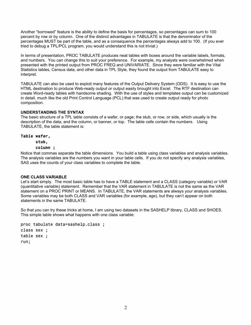
ONE CLASS VARIABLE Let’s start simply. The most basic table has to have a TABLE statement and a CLASS (category variable) or VAR (quantitative variable) statement. Remember that the VAR statement in TABULATE is not the same as the VAR statement on a PROC PRINT or MEANS. In TABULATE, the VAR statements are always your analysis variables. Some variables may be both CLASS and VAR variables (for example, age), but they can’t appear on both statements in the same TABULATE. So that you can try these tricks at home, I am using two datasets in the SASHELP library, CLASS and SHOES. This simple table shows what happens with one class variable: proc tabulate data=sashelp.class ; class sex ; table sex ; run;

2

Produces this output:

Whoa! What happened? The default statistic for a class variable is N – a count of the observations.

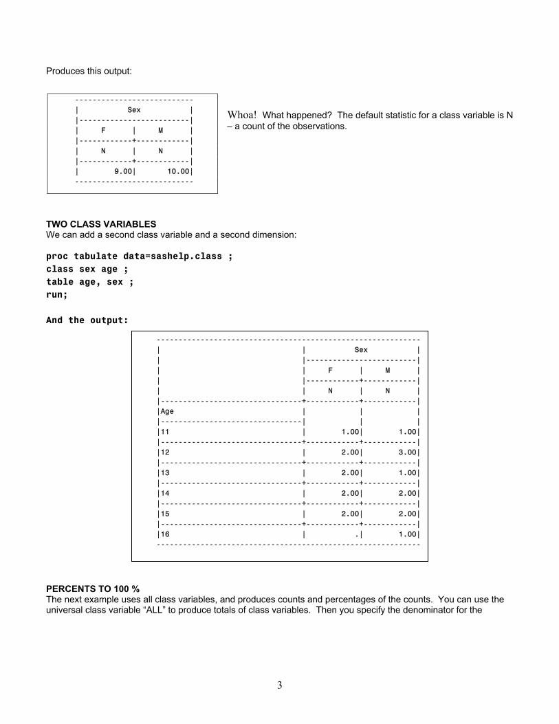
TWO CLASS VARIABLES We can add a second class variable and a second dimension: proc tabulate data=sashelp.class ; class sex age ; table age, sex ; run; And the output:

--------------------------- | Sex | |-------------------------| | F | M | |------------+------------| | N | N | |------------+------------| | 9.00| 10.00| ---------------------------

------------------------------------------------------------ | | Sex | | |-------------------------| | | F | M | | |------------+------------| | | N | N | |--------------------------------+------------+------------| |Age | | | |--------------------------------| | | |11 | 1.00| 1.00| |--------------------------------+------------+------------| |12 | 2.00| 3.00| |--------------------------------+------------+------------| |13 | 2.00| 1.00| |--------------------------------+------------+------------| |14 | 2.00| 2.00| |--------------------------------+------------+------------| |15 | 2.00| 2.00| |--------------------------------+------------+------------| |16 | .| 1.00| ------------------------------------------------------------

PERCENTS TO 100 % The next example uses all class variables, and produces counts and percentages of the counts. You can use the universal class variable “ALL” to produce totals of class variables. Then you specify the denominator for the

3

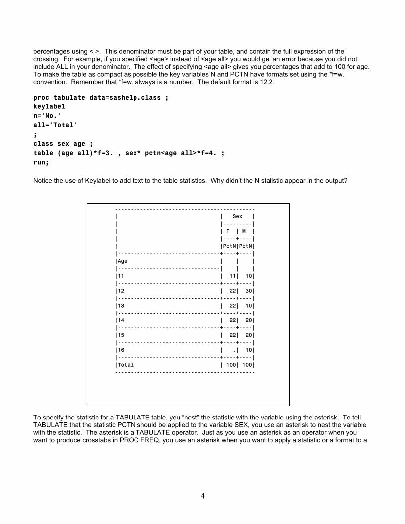
percentages using < >. This denominator must be part of your table, and contain the full expression of the crossing. For example, if you specified <age> instead of <age all> you would get an error because you did not include ALL in your denominator. The effect of specifying <age all> gives you percentages that add to 100 for age. To make the table as compact as possible the key variables N and PCTN have formats set using the *f=w. onvention. Remember that *f=w. always is a number. The default format is 12.2.

ate data=sashelp.class ;

='Total'

(age all)*f=3. , sex* pctn<age all>*f=4. ;

otice the use of Keylabel to add text to the table statistics. Why didn’t the N statistic appear in the output?

le

to a

c proc tabulkeylabel n='No.' all; class sex age ; table run; N

To specify the statistic for a TABULATE table, you “nest” the statistic with the variable using the asterisk. To tell TABULATE that the statistic PCTN should be applied to the variable SEX, you use an asterisk to nest the variabwith the statistic. The asterisk is a TABULATE operator. Just as you use an asterisk as an operator when you want to produce crosstabs in PROC FREQ, you use an asterisk when you want to apply a statistic or a format

-------------------------------------------- | | Sex | | |---------| | | F | M | | |----+----| | |PctN|PctN| |--------------------------------+----+----| |Age | | | |--------------------------------| | | |11 | 11| 10| |--------------------------------+----+----| |12 | 22| 30| |--------------------------------+----+----| |13 | 22| 10| |--------------------------------+----+----| |14 | 22| 20| |--------------------------------+----+----| |15 | 22| 20| |--------------------------------+----+----| |16 | .| 10| |--------------------------------+----+----| |Total | 100| 100| --------------------------------------------

4

variable. In version 8.2, instead of specifying PCTN and a denominator, you could just ask for ROWPCTN or COLPCTN.

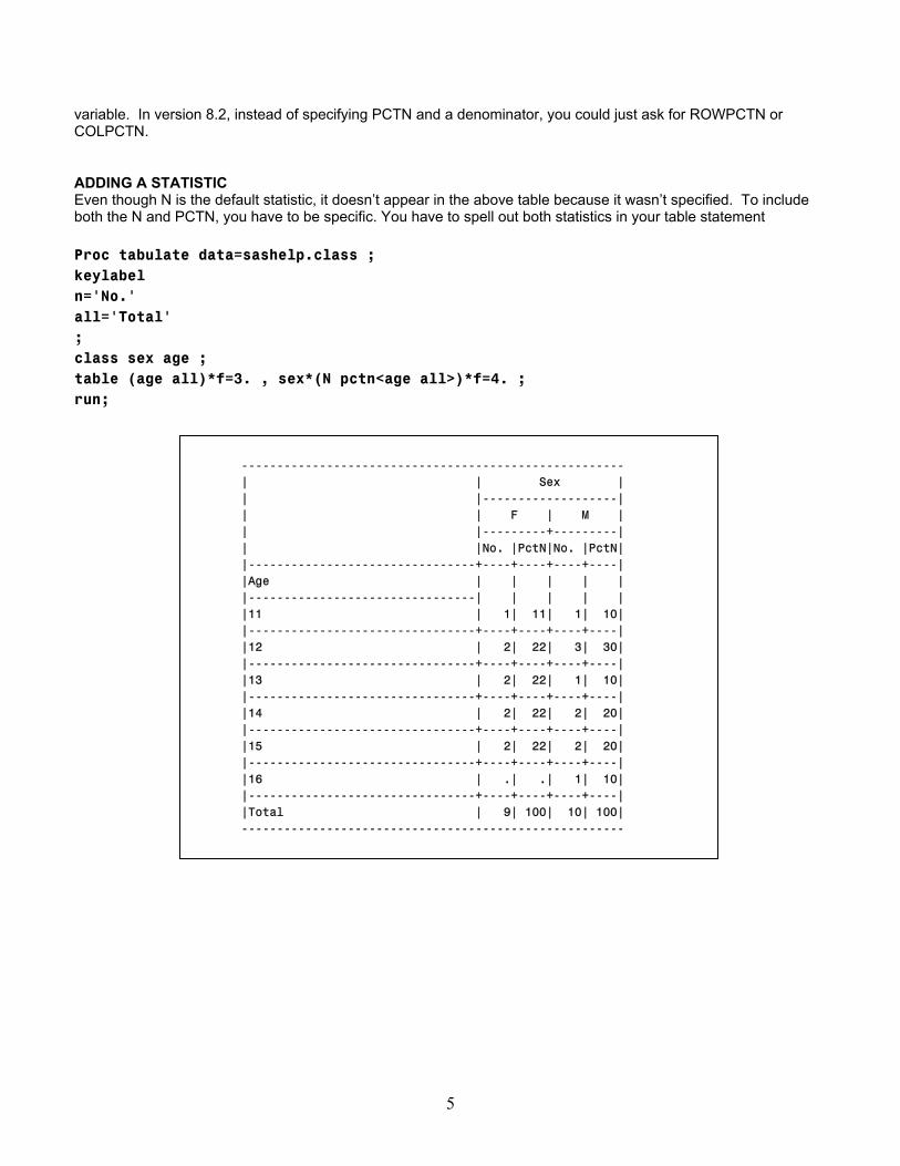
en though N is the default statistic, it doesn’t appear in the above table because it wasn’t specified. To include ou have to spell out both statistics in your table statement

late data=sashelp.class ;

No.'

sex age ; e (age all)*f=3. , sex*(N pctn<age all>)*f=4. ;

run;

ADDING A STATISTIC Evboth the N and PCTN, you have to be specific. Y Proc tabukeylabel n='all='Total' ; class tabl

------------------------------------------------------ | | Sex | | |-------------------| | | F | M | | |---------+---------| | |No. |PctN|No. |PctN| |--------------------------------+----+----+----+----| |Age | | | | | |--------------------------------| | | | | |11 | 1| 11| 1| 10| |--------------------------------+----+----+----+----| |12 | 2| 22| 3| 30| |--------------------------------+----+----+----+----| |13 | 2| 22| 1| 10| |--------------------------------+----+----+----+----| |14 | 2| 22| 2| 20| |--------------------------------+----+----+----+----| |15 | 2| 22| 2| 20| |--------------------------------+----+----+----+----| |16 | .| .| 1| 10| |--------------------------------+----+----+----+----| |Total | 9| 100| 10| 100| ------------------------------------------------------

5

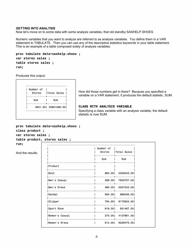
GETTING INTO ANALYSIS Now let’s move on to some data with some analysis variables, that old standby SASHELP.SHOES. Numeric variables that you want to analyze are referred to as analysis variables. You define them in a VAR statement to TABULATE. Then you can use any of the descriptive statistics keywords in your table statement. This is an example of a table composed solely of analysis variables: proc tabulate data=sashelp.shoes ; var stores sales ; table stores sales ; run; Produces this output:

How did those numbers get in there? Because you specified a variable on a VAR statement, it produces the default statistic, SUM.

CLASS WITH ANALYSIS VARIABLE Specifying a class variable with an analysis variable, the default statistic is now SUM.

--------------------------- | Number of | | | Stores |Total Sales | |------------+------------| | Sum | Sum | |------------+------------| | 4601.00| 33851566.00| ---------------------------

proc tabulate data=sashelp.shoes ; class product ; var stores sales ; table product, stores sales ; run; And the results:

---------------------------------------------------------- | | Number of | | | | Stores |Total Sales | | |------------+------------| | | Sum | Sum | |------------------------------+------------+------------| |Product | | | |------------------------------| | | |Boot | 864.00| 2350543.00| |------------------------------+------------+------------| |Men's Casual | 399.00| 7933707.00| |------------------------------+------------+------------| |Men's Dress | 480.00| 5507243.00| |------------------------------+------------+------------| |Sandal | 564.00| 868436.00| |------------------------------+------------+------------| |Slipper | 794.00| 6175834.00| |------------------------------+------------+------------| |Sport Shoe | 616.00| 651467.00| |------------------------------+------------+------------| |Women's Casual | 270.00| 4137861.00| |------------------------------+------------+------------| |Women's Dress | 614.00| 6226475.00|

6

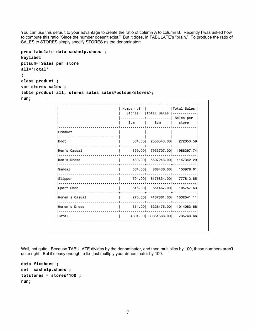
You can use this default to your advantage to create the ratio of column A to column B. Recently I was asked how to compute this ratio “Since the number doesn’t exist.” But it does, in TABULATE’s “brain.” To produce the ratio of SALES to STORES simply specify STORES as the denominator: proc tabulate data=sashelp.shoes ; keylabel pctsum='Sales per store' all='Total' ; class product ; var stores sales ; table product all, stores sales sales*pctsum<stores>; run;

----------------------------------------------------------------------- | | Number of | |Total Sales | | | Stores |Total Sales |------------| | |------------+------------| Sales per | | | Sum | Sum | store | |------------------------------+------------+------------+------------| |Product | | | | |------------------------------| | | | |Boot | 864.00| 2350543.00| 272053.59| |------------------------------+------------+------------+------------| |Men's Casual | 399.00| 7933707.00| 1988397.74| |------------------------------+------------+------------+------------| |Men's Dress | 480.00| 5507243.00| 1147342.29| |------------------------------+------------+------------+------------| |Sandal | 564.00| 868436.00| 153978.01| |------------------------------+------------+------------+------------| |Slipper | 794.00| 6175834.00| 777812.85| |------------------------------+------------+------------+------------| |Sport Shoe | 616.00| 651467.00| 105757.63| |------------------------------+------------+------------+------------| |Women's Casual | 270.00| 4137861.00| 1532541.11| |------------------------------+------------+------------+------------| |Women's Dress | 614.00| 6226475.00| 1014083.88| |------------------------------+------------+------------+------------| |Total | 4601.00| 33851566.00| 735743.66| -----------------------------------------------------------------------

Well, not quite. Because TABULATE divides by the denominator, and then multiplies by 100, these numbers aren’t quite right. But it’s easy enough to fix, just multiply your denominator by 100. data fixshoes ; set sashelp.shoes ; totstores = stores*100 ; run;

7

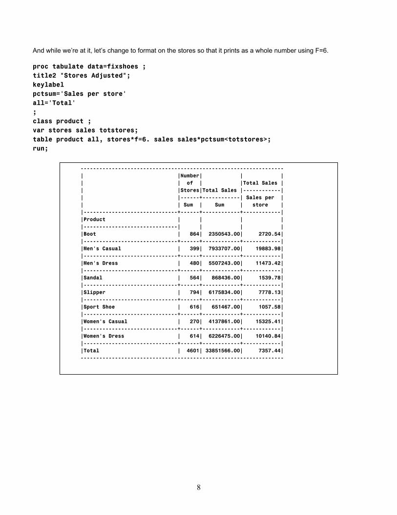
And while we’re at it, let’s change to format on the stores so that it prints as a whole number using F=6. proc tabulate data=fixshoes ; title2 "Stores Adjusted"; keylabel pctsum='Sales per store' all='Total' ; class product ; var stores sales totstores; table product all, stores*f=6. sales sales*pctsum<totstores>; run;

----------------------------------------------------------------- | |Number| | | | | of | |Total Sales | | |Stores|Total Sales |------------| | |------+------------| Sales per | | | Sum | Sum | store | |------------------------------+------+------------+------------| |Product | | | | |------------------------------| | | | |Boot | 864| 2350543.00| 2720.54| |------------------------------+------+------------+------------| |Men's Casual | 399| 7933707.00| 19883.98| |------------------------------+------+------------+------------| |Men's Dress | 480| 5507243.00| 11473.42| |------------------------------+------+------------+------------| |Sandal | 564| 868436.00| 1539.78| |------------------------------+------+------------+------------| |Slipper | 794| 6175834.00| 7778.13| |------------------------------+------+------------+------------| |Sport Shoe | 616| 651467.00| 1057.58| |------------------------------+------+------------+------------| |Women's Casual | 270| 4137861.00| 15325.41| |------------------------------+------+------------+------------| |Women's Dress | 614| 6226475.00| 10140.84| |------------------------------+------+------------+------------| |Total | 4601| 33851566.00| 7357.44| -----------------------------------------------------------------

8

FORMATTING AND ORDERING CLASS VARIABLES How can you get class variables in an order other than sorted order? Suppose you define a format as: proc format ; value $regfmt 'United States','Canada' = 'USA & Canada' 'Central America/Caribbean','South America' = 'South/Central America' 'Western Europe','Eastern Europe' = 'Europe' 'Pacific', 'Asia' = 'Asia and Pacific Islands' other = 'Elsewhere' ; run; and use it with the previous TABULATE. The resulting output has the class “Elsewhere” first, then Asia and Pacific Islands. Even though you typed them in the order that you wanted, SAS goes ahead and sorts them internally. To get the order that you want, use the (NOTSORTED) option on your format: proc format fmtlib; value $regfmt (notsorted) 'United States','Canada' = 'USA & Canada' 'Central America/Caribbean','South America' = 'South/Central America' 'Western Europe','Eastern Europe' = 'Europe' 'Pacific', 'Asia' = 'Asia and Pacific Islands' other = 'Elsewhere' ; run; and specify order = data on your tabulate statement: proc tabulate data=fixshoes order=data ; keylabel pctsum='Sales per store' all='Total' ; class region /preloadfmt ; class product ; var stores sales totstores; table region*(product all), stores*f=6. sales sales*pctsum<totstores> /rts=40; format region $regfmt. ; run;

9

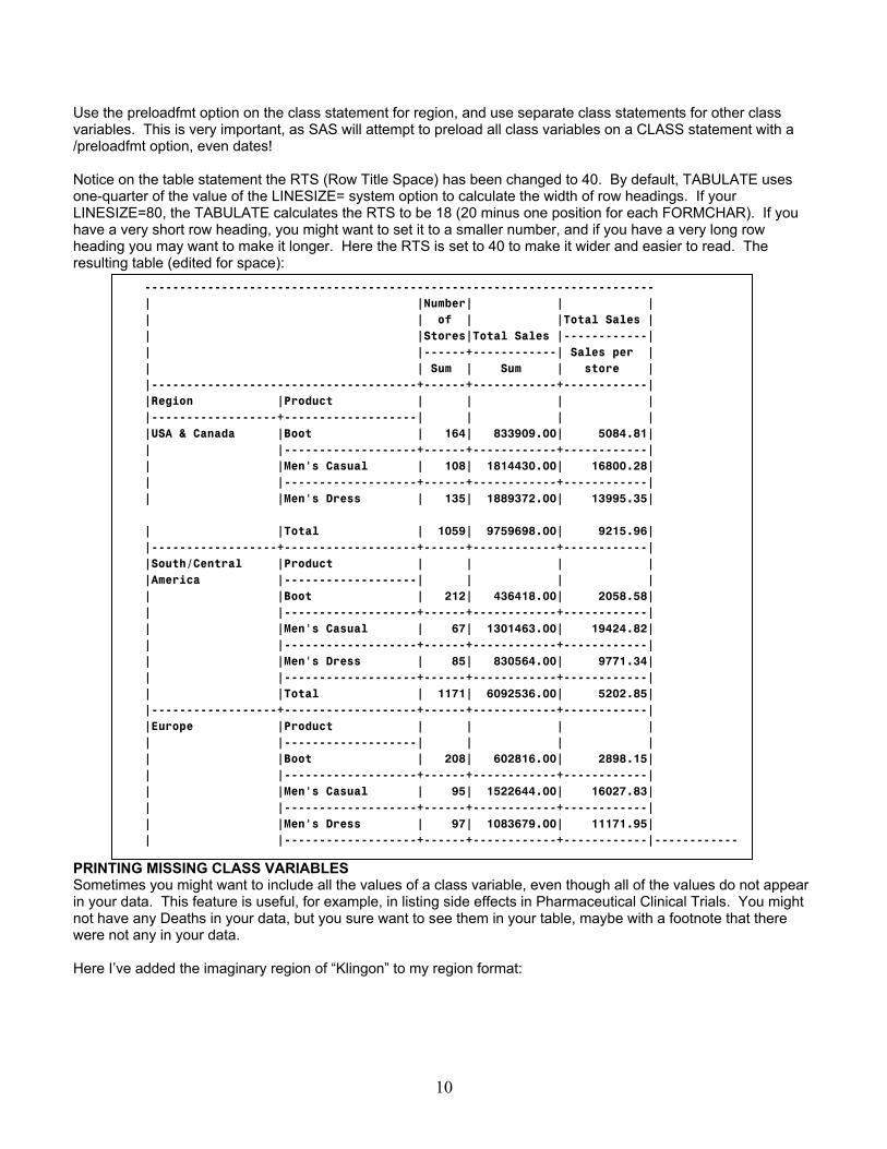
Use the preloadfmt option on the class statement for region, and use separate class statements for other class variables. This is very important, as SAS will attempt to preload all class variables on a CLASS statement with a /preloadfmt option, even dates! Notice on the table statement the RTS (Row Title Space) has been changed to 40. By default, TABULATE uses one-quarter of the value of the LINESIZE= system option to calculate the width of row headings. If your LINESIZE=80, the TABULATE calculates the RTS to be 18 (20 minus one position for each FORMCHAR). If you have a very short row heading, you might want to set it to a smaller number, and if you have a very long row heading you may want to make it longer. Here the RTS is set to 40 to make it wider and easier to read. The resulting table (edited for space):

PRINTSometin yournot hawere n Here I’

------------------------------------------------------------------------- | |Number| | | | | of | |Total Sales | | |Stores|Total Sales |------------| | |------+------------| Sales per | | | Sum | Sum | store | |--------------------------------------+------+------------+------------| |Region |Product | | | | |------------------+-------------------| | | | |USA & Canada |Boot | 164| 833909.00| 5084.81| | |-------------------+------+------------+------------| | |Men's Casual | 108| 1814430.00| 16800.28| | |-------------------+------+------------+------------| | |Men's Dress | 135| 1889372.00| 13995.35| | |Total | 1059| 9759698.00| 9215.96| |------------------+-------------------+------+------------+------------| |South/Central |Product | | | | |America |-------------------| | | | | |Boot | 212| 436418.00| 2058.58| | |-------------------+------+------------+------------| | |Men's Casual | 67| 1301463.00| 19424.82| | |-------------------+------+------------+------------| | |Men's Dress | 85| 830564.00| 9771.34| | |-------------------+------+------------+------------| | |Total | 1171| 6092536.00| 5202.85| |------------------+-------------------+------+------------+------------| |Europe |Product | | | | | |-------------------| | | | | |Boot | 208| 602816.00| 2898.15| | |-------------------+------+------------+------------| | |Men's Casual | 95| 1522644.00| 16027.83| | |-------------------+------+------------+------------| | |Men's Dress | 97| 1083679.00| 11171.95| | |-------------------+------+------------+------------|------------

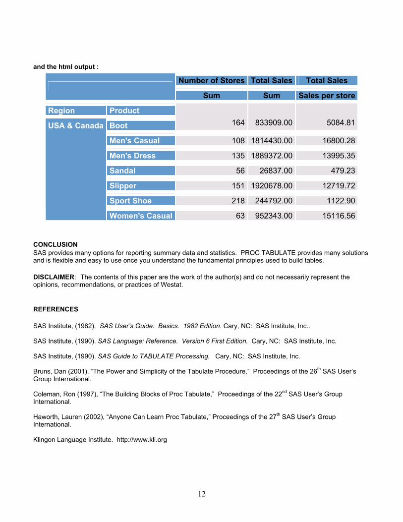
ING MISSING CLASS VARIABLES imes you might want to include all the values of a class variable, even though all of the values do not appear data. This feature is useful, for example, in listing side effects in Pharmaceutical Clinical Trials. You might ve any Deaths in your data, but you sure want to see them in your table, maybe with a footnote that there ot any in your data.

ve added the imaginary region of “Klingon” to my region format:

10

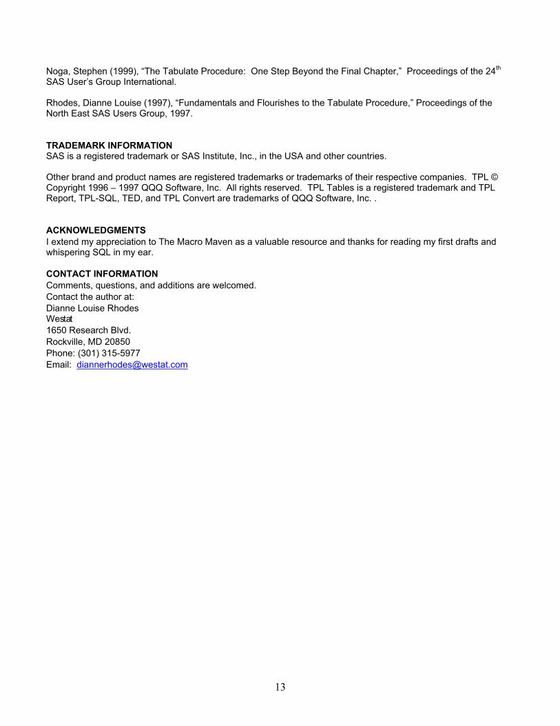
proc format fmtlib; value $regfmt (notsorted) 'United States','Canada' = 'USA & Canada' etc.. 'Klingon' = 'Klingon' Other = 'Every where Else' ; And while we’re at it, let’s wrap some ODS destinations around the code and create HTML output: ods html body='Advanced1.html' style=barrettsblue ; proc tabulate data=fixshoes order=data ; keylabel pctsum='Sales per store' all='Total' ; class region /preloadfmt ; class product ; var stores sales ; table region*(product all), stores*f=6. sales sales*pctsum<totstores> /rts=40 printmiss misstext='**'; format region $regfmt. ; *footnote1 "** Not available at this time"; run; ods html close ; Notice that I did not close the listing destination. I prefer to have my listing output in addition to my ODS HTML or RTF output. It is much easier for me to check it in TextPad, whereas to check the RTF or HTML I have to open Word or a browser. Specifying the printmiss and misstext options tells TABULATE to print those rows with missing data and use the text in misstext to display them. This adds this section to the table;

|------------------+-------------------+------------+------------+------------| |Klingon |Product | | | | | |-------------------| | | | | |Boot | **| **| **| | |-------------------+------------+------------+------------| | |Men's Casual | **| **| **| | |-------------------+------------+------------+------------| | |Men's Dress | **| **| **| | |-------------------+------------+------------+------------| | |Sandal | **| **| **| |------------------+-------------------+------------+------------+------------|

11

and the html output :

Number of Stores Total Sales Total Sales

Sum Sum Sales per store

Region Product

Boot 164 833909.00 5084.81

Men's Casual 108 1814430.00 16800.28

Men's Dress 135 1889372.00 13995.35

Sandal 56 26837.00 479.23

Slipper 151 1920678.00 12719.72

Sport Shoe 218 244792.00 1122.90

USA & Canada

Women's Casual 63 952343.00 15116.56

CONCLUSION SAS provides many options for reporting summary data and statistics. PROC TABULATE provides many solutions and is flexible and easy to use once you understand the fundamental principles used to build tables. DISCLAIMER: The contents of this paper are the work of the author(s) and do not necessarily represent the opinions, recommendations, or practices of Westat.

REFERENCES SAS Institute, (1982). SAS User’s Guide: Basics. 1982 Edition. Cary, NC: SAS Institute, Inc.. SAS Institute, (1990). SAS Language: Reference. Version 6 First Edition. Cary, NC: SAS Institute, Inc. SAS Institute, (1990). SAS Guide to TABULATE Processing. Cary, NC: SAS Institute, Inc. Bruns, Dan (2001), “The Power and Simplicity of the Tabulate Procedure,” Proceedings of the 26th SAS User’s Group International. Coleman, Ron (1997), “The Building Blocks of Proc Tabulate,” Proceedings of the 22nd SAS User’s Group International. Haworth, Lauren (2002), “Anyone Can Learn Proc Tabulate,” Proceedings of the 27th SAS User’s Group International. Klingon Language Institute. http://www.kli.org

12

13

Noga, Stephen (1999), “The Tabulate Procedure: One Step Beyond the Final Chapter,” Proceedings of the 24th SAS User’s Group International. Rhodes, Dianne Louise (1997), “Fundamentals and Flourishes to the Tabulate Procedure,” Proceedings of the North East SAS Users Group, 1997.

TRADEMARK INFORMATION SAS is a registered trademark or SAS Institute, Inc., in the USA and other countries. Other brand and product names are registered trademarks or trademarks of their respective companies. TPL © Copyright 1996 – 1997 QQQ Software, Inc. All rights reserved. TPL Tables is a registered trademark and TPL Report, TPL-SQL, TED, and TPL Convert are trademarks of QQQ Software, Inc. .

ACKNOWLEDGMENTS I extend my appreciation to The Macro Maven as a valuable resource and thanks for reading my first drafts and whispering SQL in my ear.

CONTACT INFORMATION Comments, questions, and additions are welcomed. Contact the author at: Dianne Louise Rhodes Westat 1650 Research Blvd. Rockville, MD 20850 Phone: (301) 315-5977 Email: diannerhodes@westat.com