SPE 160171

Combined Uncertainty and History Matching Study of a Deepwater Turbidite Reservoir Akshay Aggarwal (*), Song Du, and Michael J. King, Department of Petroleum Engineering, Texas A&M University, (*) Currently at Schlumberger

Copyright 2012, Society of Petroleum Engineers This paper was prepared for presentation at the SPE Annual Technical Conference and Exhibition held in San Antonio, Texas, USA, 8-10 October 2012. This paper was selected for presentation by an SPE program committee following review of information contained in an abstract submitted by the author(s). Contents of the paper have not been reviewed by the Society of Petroleum Engineers and are subject to correction by the author(s). The material does not necessarily reflect any position of the Society of Petroleum Engineers, its officers, or members. Electronic reproduction, distribution, or storage of any part of this paper without the written consent of the Society of Petroleum Engineers is prohibited. Permission to reproduce in print is restricted to an abstract of not more than 300 words; illustrations may not be copied. The abstract must contain conspicuous acknowledgment of SPE copyright.

Abstract A textbook description of history matching could indicate that it is a process wherein changes are made to an initial geologic model of a reservoir, so that the predicted reservoir performance matches with the known production history. A practitioner recognizes that this is an overly simplistic description: (1) Does not recognize subsurface uncertainty and how we may explore this uncertainty with multiple geologic models. (2) Offers no guidance on the requirements of spatial resolution, and how this choice may vary depending the stage of field life or reservoir processes, e.g., a pressure history match versus the modeling of a secondary or tertiary process. (3) Offers no guidance on the nature of the geologic model: its characteristics, its level of detail, or its structure. (4) Provides no description of the history matching process itself, nor the choices available to a practitioner.

We have been supplied with the historical field data for a deepwater turbidite reservoir, which is still under active development. We have used this reservoir to explore a number of history matching strategies. This project involved an integrated seismic to simulation study, wherein we interpreted the seismic data, assembled the geological information, performed petrophysical log evaluation and well test pressure transient analysis before creating the 3D geologic model.

In the matching process we examined the trade-off between exploring a wide number of models versus calibrating a single model. We examined the scale at which the geologic model was constructed, and how the scale of simulation could be determined. Finally, we studied both the large discrete steps in the process, and the smaller local "assisted" parameter calibration. The results provide general guidance on workflow sequence, guidance on model selection, and guidance on the scales of static and dynamic modeling. We expect many of these conclusions to have general utility, not restricted to this specific study. Introduction History matching is a process wherein changes are made to one or more initial geologic models of a reservoir, so that the predicted reservoir performance matches with the known production history. The purpose of the history match is to obtain calibrated reservoir descriptions which may then be used for performance prediction and reservoir management decisions. The initial geologic model provides a representation of the reservoir structure, its stratigraphy, layering, sedimentology and facies distribution. The static model consists of a three dimensional spatial distribution of porosity and permeability derived from this geologic model. This static model is then filled with an initial fluid distribution of water, oil and/or gas within the flow simulator. Historical well, injection and a subset of production data are used to provide the boundary conditions for reservoir simulation performance prediction, and the remaining production and pressure data is used to test those predictions. The intent of our current study is to emphasize the importance of multiple initial geologic models and to demonstrate an uncertainty assessment strategy based upon multiple geologic interpretations. The uncertainty assessment is a precursor to a full history matching study. It may be thought of as a means of generating multiple starting points for history matching model calibration, or, perhaps more importantly, it may be used to obtain an improved reservoir description even without the full implementation of a history match.

We will not attempt to review the history matching literature. The recent reprint collection (Datta-Gupta 2009) provides an excellent starting point to understand current, developing and historical practice. However, we will cite a number of publications which we have found to be especially influential because of their impact on the current work. The “Stratigraphic Method” (Williams et.al. 1998) emphasizes a systematic approach based on increasing resolution from Global to Flow Unit

2 SPE 160171

to Layer to Well. It also implies a systematic change in conditioning data with the Global stage of the match emphasizing the reservoir energy (volumes, rock and fluid compressibility, aquifer support), the Flow Unit / Layer stages emphasizing flood front progression (permeability, permeability barriers, permeability contrast, relative permeability), and the Layer / Well stages detailed well pressures and rates and water-cut development (near well permeability, well skins). A similar progression will be used in the current history matching study.

BP’s TDRM™ approach (Williams et.al. 2004) places history matching in the context of decision support, with an overall workflow consisting of Business Issue, Uncertainty Definition, Appropriate Model and Simulator, History Matching, Depletion Planning, and finally, Decision. It recognizes that the choice of an appropriate model, or in fact, an appropriate solution, may very well be case specific. For instance, decisions made at the time of project sanction or early in field life may be dominated by subsurface or project uncertainty, and may not require high resolution reservoir simulation calculations. Of course, such a conclusion will be case specific, but it offers useful guidance that simple models may provide sufficient insight to support business decisions. It also recognizes that the use of too few interpretations may lead to anchoring of the models and too little exploration of subsurface possibilities. The current study benefits from these insights and will explore the use of multiple geologic interpretations and models, with varying degrees of simplicity and complexity, as well as various degrees of spatial resolution (low to high). We find that this is a very effective way of learning about the reservoir, even before the history matching process begins.

With the development of Assisted History Matching (AHM) techniques, it has become possible to treat history matching as an optimization process in which the mis-match between prediction and history is minimized. In principle this allows multiple initial models and the multiple stages of the Stratigraphic Method to be optimized (matched) simultaneously. Such a methodology has been studied in a recent work (Cheng et.al. 2008) given the significant range of technologies now available: experimental design, proxy models, gradient and sensitivity based formal optimization, genetic or evolutionary approaches, streamline-based inversion, EnKF, and so on. They have found significant benefit in following a sequence of stages so that the most important and global parameters are estimated early in a study and less important or localized parameters are calibrated later. Without such a structured approach, the AHM techniques may provide spurious results, which are optimal only in the sense of minimizing a misfit function but which do not provide reasonable reservoir descriptions or reasonable performance predictions. These effects will be demonstrated in the current study, especially as we look at the interplay between the AHM techniques and models that have, perhaps, too simplistic a geologic description.

This paper describes the history match within an integrated seismic to simulation research study, including the interpretation of the seismic data, assembly of the geological information, petrophysical log evaluation and well test pressure transient interpretation. We will use the results of this integrated geoscience study as the starting point for the history match.

The following general conclusions were drawn from this study: a) The use of multiple simple geologic models is extremely useful in screening possible geologic scenarios and

especially for discarding unreasonable alternative models. This was especially true when developing an understanding of the large scale architecture of the reservoir.

b) The AHM methodology was very effective in exploring a large number of parameters, running the simulation cases, and generating the calibrated reservoir models. The calibration step consistently worked better if the models had more spatial detail, instead of the more homogeneous models used for the initial screening.

c) Our implementation of the AHM methodology followed a sequence of pressure and water cut history matching. An examination of specific models indicated that those cases which minimized the conflict between these two match criteria also provided a better geologic description.

The field data for our study has been provided by a major oil and gas producer for research and educational purposes. However, this study has been performed without their direct intervention. All conclusions are our own, and do not reflect on the operator. Some information in this study has been obtained from the literature related to this specific field. However, we have refrained from citing those references to the literature for reasons of confidentiality.

This paper is organized as follows. In the next section we review the specific history matching methodologies which will be applied in this study. This is followed by a review of the field history and initial reservoir description. This leads to the major portions of our paper: the uncertainty study, the history match and the final reservoir description. Our reservoir-specific results are then described and general conclusions on methodology are provided. Most of the applications used in this study are commercially available. They will be cited by name for completeness, but the most important results concerning strategies in the use of multiple geologic interpretations impact how the tools are used and are application independent. Methodology This project involved an integrated seismic to simulation study, including horizon and fault interpretation from the seismic data, assembly of the geological information, petrophysical log evaluation and well test pressure transient interpretation. The interpreted seismic data is used to build the horizons and faults for the structural model of the field, which was subsequently used to construct a three dimensional gridded geologic model. These aspects of our study are conventional and are not described in any detail. Use was made of Landmark’s GeoGraphix (GeoGraphix 2012) for seismic interpretation, petrophysical analysis, and reservoir mapping. The 3D grid and geologic model properties were constructed using Roxar’s Reservoir Modeling System (RMS 2012) for static modeling and property upscaling for flow simulation. Dynamic

SPE 160171 3

predictions were performed using Schlumberger’s ECLIPSE 100 simulator (ECLIPSE 2011). The MEPO application, provided by the SPT Group (MEPO 2012), was used for the parameter sensitivities and Assisted History Matching, of reservoir energy. The water cut history match was performed using the streamline-based Generalized Travel Time Inversion technique in the in-house developed DESTINY application (MCERI 2011). Use was also made of the in-house developed SWIFT application (MCERI 2011) for flow simulation layering design.

The uncertainty study starts with a methodology documented for the Magnus reservoir (Moulds et.al. 2005). This is a diagrammatic approach in which the major subsurface uncertainties are displayed visually. This is a very useful approach to assist in creating a sufficiently broad range of starting models. It also provides rapid documentation in post-project reviews in the sense that uncertainties that do not appear in this visual display were not considered within the study. The second stage of our uncertainty study is based on the calculation of the objective function which measures the mis-match between historical and predicted for each of these models. We have found this combination of qualitative and quantitative analysis to provide excellent insight into the reservoir description, even before starting a full history match.

The first stage of the history match is performed using MEPO (Schulze-Riegert et.al. 2003). In this style of reservoir characterization, the field is subdivided into regions, which may correspond to geologic units, facies types, or other areal divisions. On each of these regions properties, typically porosity and permeability, may be modified independently. Initially a screening study is performed, possibly under the control of an experimental design, from which we obtain a ranking of the importance of each of these parameters (Box and Draper 1987, Eide et.al. 1994, White et.al. 2001, White and Royer 2003). The highest ranking subset of parameters is then utilized to minimize the mismatch objective function with an evolutionary strategy (Back 1996, Back and Schwefel 1997, Cheng et.al. 2008).

These techniques will provide one or more set of parameters which are optimal in the sense that they minimize a misfit function. However, in terms of providing a reservoir characterization, the spatial resolution of the parameter changes is limited by the initial region definitions. At best, these parameters, or their changes, must be thought of as averages over each region. Attempting to redefine regions, or including additional degrees of freedom for increased spatial resolution on regions, is an active area of research (Xie et.al. 2010, Bhark et.al. 2011). In the later stages of our history match, we will increase the number of regions, guided by the performance of the history match.

In contrast, streamline-based analysis techniques do not rely upon pre-defined region definitions, but instead utilize bundles of streamlines for dynamic region definitions (Milliken et.al. 2001). This concept may be extended further by using the streamlines to calculate spatial sensitivity information which describes how a change in the permeability of any cell in the model contributes to a change of water-cut at each well (Vasco et.al. 1999, Wu et.al. 2002). This sensitivity information may be combined with the mismatch in water-cut progression at each well to determine changes in permeability within the reservoir model. To ensure uniqueness in these cell by cell changes the inversion is regularized by constraining it to have minimum changes from the prior geologic model together with a smoothness constraint. These techniques are related to the formal inversion techniques used in geophysical travel time inversion (Luo and Schuster 1991). As a reservoir characterization tool, changes are made in the prior model driven by the spatial data support of the well data. No previously defined regions are required. However, these techniques are based upon convective processes, and work best to modify transport properties, i.e., permeability, once a water-cut matures. In contrast, variation of properties on regions may be used to modify both porosity and permeability, e.g., volumes and transport.

Our overall methodology is summarized in Figure 1. We have just described the techniques or applications that we will use in this workflow. Each individual element of this workflow is commercially available or has been previously demonstrated in other research papers. However, to emphasize those elements which are most unique to the current study, let us summarize each element in turn.

Create Initial Set of Geologic Models

We wish to emphasize that this is not a matter of drawing multiple realizations from a single geologic interpretation. Instead it is a creative activity in which multiple geologic interpretations are created or major geologic features are varied. The wider the range of interpretations created, the more informative the uncertainty study will be. In fact, it is beneficial to create “unreasonable” geologic interpretations simply to demonstrate the impact that these distinct interpretations would have on our performance predictions. However, in so far as our dynamic data provides insight into our geologic description, this information will be included in the models constructed. Specifically, pressure transient well test analysis provides distance to barriers for each well, which will be used for the characteristic sizes of channels, for any of the channelized reservoir models. In addition, mass balance analysis provides information on aquifer size and aquifer communication before performing the history match.

Multiple realizations of each geologic interpretation may be created, but our experience has shown that the breadth in reservoir descriptions and performance predictions are driven by the breadth of the set of geologic models, not by the number of realizations within each interpretation. To simplify our current study, we will work with only a single realization for each interpretation. We recognize that if we were the field operator, that we would have introduced multiple realizations either as part of the history matching workflow, in the subsequent performance predictions, or both.

4 SPE 160171

Figure 1: Overall Uncertainty and History Matching Methodology Uncertainty Study: Screen Models to Obtain a Subset for History Matching

Here we utilize part of the technology of a history matching workflow, although without performing the history match itself. We define an objective function as the weighted sum of the differences between field data and performance prediction, versus time. Specifically we compare the simulated and predicted bottom hole flowing pressure of the wells to obtain our initial global error measure. Inclusion of the water-cut error complicates this analysis and does not seem to provide additional insight to the screening of models at this stage in this uncertainty study. We will create 32 distinct geologic models and reduce them to 3 models at this stage in our study. Each model is the initial geologic model for a full history matching study. Define Regions and Parameter Ranges

Based upon our prior geologic concepts and the insight from the uncertainty study, our initial set of spatial regions are defined. We deliberately start with fairly few and fairly large regions, and recognize that we expect to refine these regions later in the study. However, we do not wish to start with too many regions until we have a better understanding of the spatial data support of our production data. Ranges of parameter values which may be defined independently on each of these regions are drawn from laboratory, core or log data. At this point we also define a base case for the parameter values. These definitions may vary for different geologic models. Tornado Study for Parameters

A standard high-low sensitivity analysis is performed for each parameter. The objective function has now been extended to include oil production, with the simulation wells constrained on total liquid production. Until we get to our later cases, these sensitivities are dominated by the misfit in reservoir pressure. This analysis provides a ranking of those parameters which most impact the objective function. This is a standard MEPO capability when performed for a single base case. This sensitivity study is repeated for each geologic model. Use Evolutionary Algorithms to Obtain Optimal Parameter Values (Pressure History Match)

Gradient-free evolutionary algorithms are used to obtain optimal values for the subset of parameters selected from the sensitivity study. This is a standard MEPO capability, although the parameter value estimation study must be repeated for each geologic model. Again, the simulation wells are constrained on total liquid production and these sensitivities are dominated by the misfit in reservoir pressure. We may think of this stage of the history match as a pressure history match. Although MEPO can be used to perform a water-cut history match, we believe that the use of pre-defined spatial regions provides a technical limit to the utility of such a calculation; we will choose to use streamline-based techniques instead. Use Streamline-based Inversion to Obtain Improved Permeability (Water-cut History Match)

Instead of developing an objective function based upon the misfit of field response versus time, the streamline-based formal optimization techniques utilize a Generalized Travel Time Inversion (GTTI) (Vasco et.al. 1999, Wu and Datta-Gupta 2002). In its simplest form, we can consider the development of the water-cut versus time, and determine the time shift required to best align historical and predicted water-cut. This error is calculated on all wells that produce water, although the detailed implementation may become complicated depending upon the complexity of reservoir management in the field (He et.al. 2002, Rey et.al. 2009). This error is measured in units of time and indicates by how much the water production needs to be delayed or accelerated within the model. These changes are implemented along the streamlines, as previously discussed.

SPE 160171 5

Both because of changing field conditions and because of how the changes are constrained to the prior geologic model, these changes are not uniform along each streamline but will vary throughout the reservoir model. As we will see, these techniques work best when the starting model has a good pressure history match. Done?

As all practitioners know, a history match study is never complete. There are always aspects of the reservoir description which may be further improved. However, these changes in reservoir description may, or may not, impact a specific business decision. Especially if we have estimated the uncertainty in our predictions, we may have a sense of the limits of predictability for a specific reservoir at a specific stage of field life. The current approach should provide a range of predictions based upon distinct geologic interpretations. Together with multiple realizations for each interpretation, we will have an estimate of the irreducible uncertainty, irrespective of the amount of effort spent on additional calibration.

The current study is an academic one, not supporting any specific business decisions. Instead we will determine those aspects of the reservoir description which are least well determined, and ask what changes we should introduce into our next set of geologic models to improve the history match. Performance Prediction based on Calibrated Subset of Geologic Models

Our industry has moved away from performance predictions based upon a single history matched model. A single model is inadequate to represent the uncertainties in our predictions or to evaluate the corresponding business risk. Utilization of a single geologic interpretation with multiple realizations may be almost as bad. On the one hand, the range of outcomes may be too narrow since significant changes to the geologic interpretation are not considered. On the other hand, the range of outcomes may be too broad since unlike a real field, typically none of the ensemble of performance predictions have the benefit of active reservoir management, e.g., reservoir surveillance leading to identification of field extensions, management of well rates, additional well locations and well timing. This style of thorough reservoir assessment may best be performed with a few characteristic models, again, which would be supported by the current approach. Improve Region Definitions or Other Global Changes

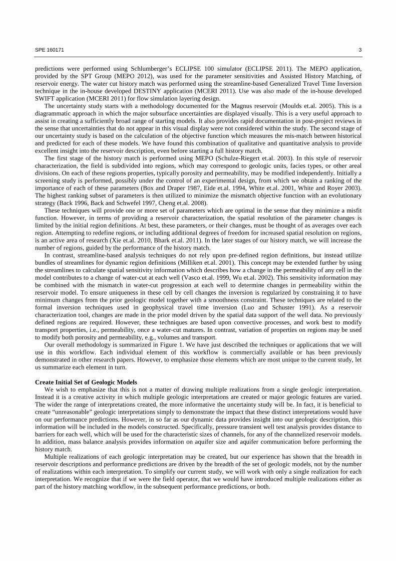
What have we learned when we’ve completed the calibration stage of a history match? There will be aspects of the initial reservoir description in which we have increased confidence and other aspects in which we will have less. In a well planned history matching study, we should have the opportunity to benefit from what we have learned by expanding or modifying the set of initial geologic models. This is especially true with the use of AHM techniques, where the actual parameter sensitivity and calibration steps may be quite short compared to the total time of a study. In our current study we will implement two styles of changes: definition of refined spatial regions and modification of the relative permeability curves. Neither of these changes was considered in the initial set of models. Field Description The reservoir being studied is a Deepwater Gulf of Mexico channelized turbidite reservoir, producing oil from the middle Miocene sands. The field has a combination of structural and stratigraphic traps. Figure 2 shows the reservoir structure of the field. It is bounded on the northeast by a W.E. fault that dips northwards, stratigraphic pinch outs on the eastern and northeastern flanks, and a salt dome lying on the western edge (Figure 3). The OWC is identified at 14300 feet from the literature survey and log evidence. The reservoir rock is composed of sand, silt and shale laminations. Information from the well logs and cores indicate that the reservoir facies can be divided into two main subcategories 1) Clean channel-fill sands, and 2) Low-quality overbank deposits. The low quality overbank deposits can be further subdivided into proximal levee and distal levee facies, which have increasing shale content. Figure 4 shows the seismic RMS amplitude map. The bright regions typically correspond to hydrocarbon presence which is generally linked to high NTG areas. Although the amplitude will dim, channel sands are expected to continue into the aquifer.

Figure 2: Top of Reservoir, showing 7 Producers and 2 Injectors, with OWC at 14300 feet

6 SPE 160171

Figure 3: M2 Top Structure Map

Figure 4: Seismic RMS Amplitude Map Draped on Top of Structure

The field is located in 5000 feet water depth. It has been developed with 9 dry-tree wells of which 7 are M-Sand producers and 2 are M-Sand injectors. The M-Sand is subdivided into three intervals (M1, M2, M3), with the bulk of the production coming from the M2 sand. Field production started in November 2002 and water injection began in September 2003. The bottom hole shut-in pressure history is shown in Figure 5.

Figure 5: Shut-In BHP pressures for all wells. With the exception of A9, all wells fall on a single trend

SPE 160171 7

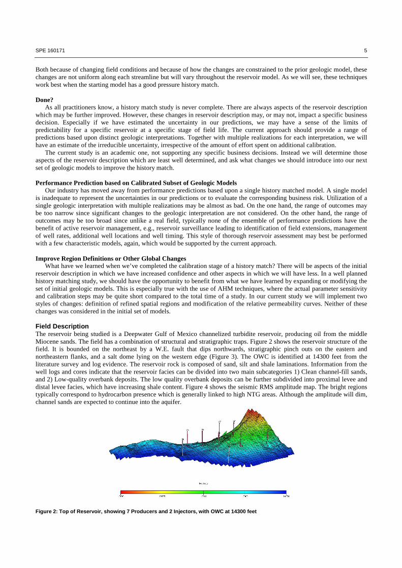
There is no evidence for compartmentalization, with the exception of the A9 well, which is the easternmost well in the field. A mass balance drive mechanism analysis has been performed from the pressure and production data, Figure 6. It shows that the single largest source of reservoir energy is aquifer influx, followed by water injection and a combination of rock and fluid compressibility.

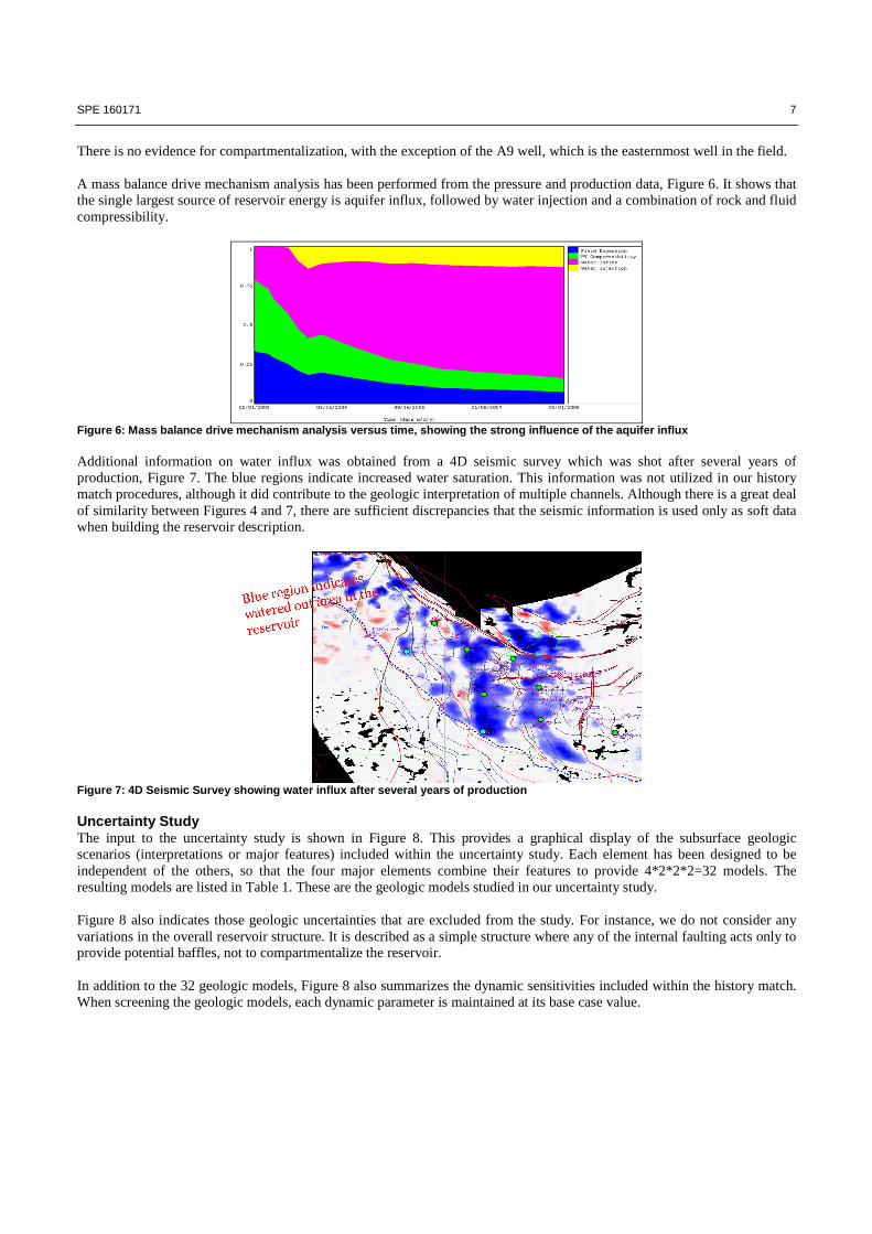
Figure 6: Mass balance drive mechanism analysis versus time, showing the strong influence of the aquifer influx Additional information on water influx was obtained from a 4D seismic survey which was shot after several years of production, Figure 7. The blue regions indicate increased water saturation. This information was not utilized in our history match procedures, although it did contribute to the geologic interpretation of multiple channels. Although there is a great deal of similarity between Figures 4 and 7, there are sufficient discrepancies that the seismic information is used only as soft data when building the reservoir description.

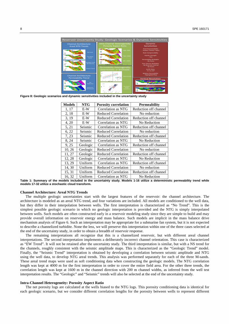
Figure 7: 4D Seismic Survey showing water influx after several years of production Uncertainty Study The input to the uncertainty study is shown in Figure 8. This provides a graphical display of the subsurface geologic scenarios (interpretations or major features) included within the uncertainty study. Each element has been designed to be independent of the others, so that the four major elements combine their features to provide 4*2*2*2=32 models. The resulting models are listed in Table 1. These are the geologic models studied in our uncertainty study. Figure 8 also indicates those geologic uncertainties that are excluded from the study. For instance, we do not consider any variations in the overall reservoir structure. It is described as a simple structure where any of the internal faulting acts only to provide potential baffles, not to compartmentalize the reservoir. In addition to the 32 geologic models, Figure 8 also summarizes the dynamic sensitivities included within the history match. When screening the geologic models, each dynamic parameter is maintained at its base case value.

8 SPE 160171

Vertical Resolution

NTG @5 layers

NTG @22 layers

Intra-Channel Heterogeneity

Porosity Aspect Ratio

1500 :10000

800 :10000

4000 :4000

Channel Architecture

Permeability Trend

No

Reduction

Reduction

Off Channel

Permeability Heterogeneity

Deterministic or Stochastic

Deterministic

Stochastic

Cloud

Transform

Channel Architecture

Areal NTG Trends

No trend

Seismic Trend

Geologic Trend

(No Seismic)

East-West

trend

Reservoir Uncertainty Study: Geologic Scenarios & Dynamic Sensitivities

Dynamic

Sensitivities

Fault Transmissibility

- Sealed / Partial / Open

Aquifer Strength

- Size

Rock Compressibility

Pore Volume Multiplier

- By Reservoir Interval

- By Facies

Permeability Multiplier

- By Facies

Relative Permeability

- Segregated Flow

Kv/Kh Ratio

- 0.1 to 10-6

Case 4 214.5

Figure 8: Geologic scenarios and dynamic sensitivities included in the uncertainty study

Models NTG Porosity correlation Permeability 1, 17 E-W Correlation as NTG Reduction off channel 2, 18 E-W Reduced Correlation No reduction 3, 19 E-W Reduced Correlation Reduction off channel 4, 20 E-W Correlation as NTG No Reduction 5, 21 Seismic Correlation as NTG Reduction off channel 6, 22 Seismic Reduced Correlation No reduction 7, 23 Seismic Reduced Correlation Reduction off channel 8, 24 Seismic Correlation as NTG No Reduction 9, 25 Geologic Correlation as NTG Reduction off channel 10, 26 Geologic Reduced Correlation No reduction 11, 27 Geologic Reduced Correlation Reduction off channel 12, 28 Geologic Correlation as NTG No Reduction 13, 29 Uniform Correlation as NTG Reduction off channel 14, 30 Uniform Reduced Correlation No reduction 15, 31 Uniform Reduced Correlation Reduction off channel 16, 32 Uniform Correlation as NTG No Reduction

Table 1: Summary of the models included in the uncertainty study. Models 1-16 utilize a deterministic permeability trend while models 17-32 utilize a stochastic cloud transform. Channel Architecture: Areal NTG Trends

The multiple geologic uncertainties start with the largest features of the reservoir: the channel architecture. The architecture is modeled as an areal NTG trend, and four variations are included. All models are conditioned to the well data, but they differ in their interpolation between wells. The first interpretation is characterized as “No Trend”. This is the simplest possible geologic scenario in which no geologic interpretation is provided and the NTG is simply interpolated between wells. Such models are often constructed early in a reservoir modeling study since they are simple to build and may provide overall information on reservoir energy and mass balance. Such models are implicit in the mass balance drive mechanism analysis of Figure 6. Such an interpretation may be appropriate for a submarine fan system, but it is not expected to describe a channelized turbidite. None the less, we will preserve this interpretation within one of the three cases selected at the end of the uncertainty study, in order to obtain a breadth of reservoir response.

The remaining interpretations all recognize that this is a channelized reservoir, but with different areal channel interpretations. The second interpretation implements a deliberately incorrect channel orientation. This case is characterized as “EW Trend”. It will not be retained after the uncertainty study. The third interpretation is similar, but with a NS trend for the channels, roughly consistent with the seismic amplitude maps. This is characterized as the “Geologic Trend” model. Finally, the “Seismic Trend” interpretation is obtained by developing a correlation between seismic amplitude and NTG using the well data, to develop NTG areal trends. This analysis was performed separately for each of the three M-sands. These areal trend maps were used as soft conditioning data when constructing the geologic models. The NTG correlation length was kept at 4000 m for the first interpretation in order to cover the entire field area. For the other three trends, the correlation length was kept at 1600 m in the channel direction with 200 m channel widths, as inferred from the well test interpretation results. The “Geologic” and “Seismic” trends will also be selected at the end of the uncertainty study. Intra-Channel Heterogeneity: Porosity Aspect Ratio

The net porosity logs are calculated at the wells biased to the NTG logs. This porosity conditioning data is identical for each geologic scenario, but we consider different correlation lengths for the porosity between wells to represent different

SPE 160171 9

amounts of intra-channel heterogeneity. Two variations are considered. In the first, the porosity has the same correlation length as the NTG. In the second, the porosity correlation length has been reduced by a factor of two in the direction of the channel width to represent proximal & distal levee facies contrast near the channel boundaries. The first variation creates models that are more homogeneous while the second are more heterogeneous. These choices are characterized as “Correlation as NTG” and “Reduced Correlation” in Table 1. At this point we now have 8 interpretations. Permeability Heterogeneity: Deterministic or Stochastic

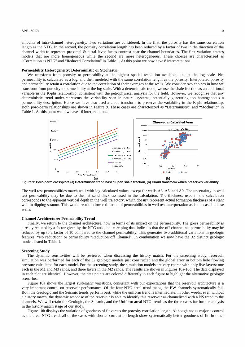
We transform from porosity to permeability at the highest spatial resolution available, i.e., at the log scale. Net permeability is calculated as a log, and then modeled with the same correlation length as the porosity. Interpolated porosity and permeability retain a correlation due to the correlation of their averages at the wells. We consider two choices in how we transform from porosity to permeability at the log scale. With a deterministic trend, we use the shale fraction as an additional variable in the K-phi relationship, consistent with the petrophysical analysis for the field. However, we recognize that any deterministic trend under-represents the variability seen in natural systems, potentially generating too homogeneous a permeability description. Hence we have also used a cloud transform to preserve the variability in the K-phi relationship. Both poro-perm relationships are shown in Figure 9. These cases are characterized as “Deterministic” and “Stochastic” in Table 1. At this point we now have 16 interpretations.

(a) (b)

Figure 9: Poro-perm crossplots (a) Deterministic trend based upon shale fraction, (b) Cloud transform which preserves variability The well test permeabilities match well with log calculated values except for wells A3, A5, and A9. The uncertainty in well test permeability may be due to the net sand thickness used in the calculation. The thickness used in the calculation corresponds to the apparent vertical depth in the well trajectory, which doesn’t represent actual formation thickness of a slant well in dipping stratum. This would result in low estimation of permeabilities in well test interpretation as is the case in these wells. Channel Architecture: Permeability Trend

Finally, we return to the channel architecture, now in terms of its impact on the permeability. The gross permeability is already reduced by a factor given by the NTG ratio, but core plug data indicates that the off-channel net permeability may be reduced by up to a factor of 10 compared to the channel permeability. This generates two additional variations in geologic features: “No reduction” or permeability “Reduction off Channel”. In combination we now have the 32 distinct geologic models listed in Table 1. Screening Study

The dynamic sensitivities will be reviewed when discussing the history match. For the screening study, reservoir simulation was performed for each of the 32 geologic models just constructed and the global error in bottom hole flowing pressure calculated for each model. For the screening study, the simulation models are very coarse with only five layers: one each in the M1 and M3 sands, and three layers in the M2 sands. The results are shown in Figures 10a-10d. The data displayed in each plot are identical. However, the data points are colored differently in each figure to highlight the alternative geologic scenarios.

Figure 10a shows the largest systematic variations, consistent with our expectations that the reservoir architecture is a very important control on reservoir performance. Of the four NTG areal trend maps, the EW channels systematically fail. Both the Geologic and the Seismic trends perform best, while the uniform trend is intermediate. In other words, even without a history match, the dynamic response of the reservoir is able to identify this reservoir as channelized with a NS trend to the channels. We will retain the Geologic, the Seismic, and the Uniform areal NTG trends as the three cases for further analysis in the history match stage of our study.

Figure 10b displays the variation of goodness of fit versus the porosity correlation length. Although not as major a control as the areal NTG trend, all of the cases with shorter correlation length show systematically better goodness of fit. In other

10 SPE 160171

words, those cases with more porosity heterogeneity provide consistently better reservoir descriptions than the more homogeneous descriptions. Since it does not lead to a significant variation in response, but does lead to systematically better response, only the shorter porosity correlation length cases will be retained for the history match.

Figure 10c examines the impact of the poro-perm correlation. As with the porosity correlation length, the models with more permeability heterogeneity perform systematically better than those constructed with a deterministic permeability trend. Again, since it does not lead to a significant variation in response, but does lead to systematically better response, only the stochastic cloud transform poro-perm cases will be retained for the history match.

Finally, Figure 10d examines the impact of the off-channel permeability reduction. There is a significant and clear indication that the models with off-channel permeability reduction perform best. Only these models will be retained in the history match.

1.36E+08

1.38E+08

1.40E+08

1.42E+08

1.44E+08

1.46E+08

1.48E+08

1.50E+08

1.52E+08

1.54E+08

1.56E+08

1.58E+08

1.60E+08

0 2 4 6 8 10 12 14 16 18 20 22 24 26 28 30 32

Glo

ba

l

Static Model

E-W Seismic Geologic Uniform

1.36E+08

1.38E+08

1.40E+08

1.42E+08

1.44E+08

1.46E+08

1.48E+08

1.50E+08

1.52E+08

1.54E+08

1.56E+08

1.58E+08

1.60E+08

0 2 4 6 8 10 12 14 16 18 20 22 24 26 28 30 32

Glo

ba

l

Static Model

Same Correlation Reduced Correlation

(a) (b)

1.36E+08

1.38E+08

1.40E+08

1.42E+08

1.44E+08

1.46E+08

1.48E+08

1.50E+08

1.52E+08

1.54E+08

1.56E+08

1.58E+08

1.60E+08

0 2 4 6 8 10 12 14 16 18 20 22 24 26 28 30 32

Glo

ba

l

Static Model

Deterministic Probabilistic

1.36E+08

1.38E+08

1.40E+08

1.42E+08

1.44E+08

1.46E+08

1.48E+08

1.50E+08

1.52E+08

1.54E+08

1.56E+08

1.58E+08

1.60E+08

0 2 4 6 8 10 12 14 16 18 20 22 24 26 28 30 32

Glo

ba

l

Static Model

No Reduction Reduction off channel

(c) (d) Figure 10: Goodness of Fit for the Uncertainty Study Versus: (a) Areal NTG Trend, (b) Porosity Correlation Length, (c) Poro-Perm Trend, and (d) Off-Channel Permeability Trend The uncertainty study has taught us a great deal about this reservoir even without performing a history match. The large scale reservoir architecture is consistent with a channelized reservoir with a NS trend to the channels. The channels control not only the quantity of sand but also the reservoir quality, with a potential order of magnitude reduction in net permeability in the off channel portions of the reservoir. Within each channel, the more heterogeneous trends in both porosity and permeability consistently perform better, even with the fairly coarse five layers models used in the screening study. The creation of multiple and distinct geologic models has allowed us to infer many geologic features directly from the production data. This is extremely encouraging as we consider deeper subsalt prospects with potentially few seismic attributes being available to provide the equivalent of “Seismic” trends. History Match In this section we will review the dynamic sensitivities and then the sequence of cases studies in the history match. The base case dynamic sensitivities have already been utilized in the uncertainty study. Each history match case will consist of four stages: the identification of one of the three geologic scenarios, a sensitivity run to determine the most important parameters, a pressure history match providing calibrated values for average properties on spatial regions and finally a water-cut history match based upon streamline sensitivities. These stages have been previous described when discussing our methodology.

SPE 160171 11

Dynamic Sensitivities Fault Transmissibility The faults in the reservoir do not separate the reservoir into separate fault blocks. Therefore, the fluid flow is not believed

to be affected by the faults. Only the fault present between wells A2 and A8 might affect the fluid flow to well A2. So, we have specified zero transmissibility across the faults for base case and kept the faults open as the other limit.

Rock Compressibility The rock compressibility value for the base case was established at 13.88x10-6 1/psi from the laboratory rock

compressibility and net confining pressure data. When plotted, the average rock compressibility for the major production time period comes out to be 13.88x10-6 1/psi. For the uncertainty analysis, we kept the rock compressibility in the range from 1x10-6 1/psi to 30x10-6 1/psi.

Aquifer Strength We used a Carter Tracy aquifer in the simulation study. The aquifer connections were made to all the cells at the oil water

contact. The aquifer permeability, thickness and encroachment angle were fixed to be the same values as determined in the material balance study. However, there was considerable uncertainty associated with the strength of the reservoir. Based on a few manual runs, the aquifer radius was varied from 300 feet (low active) to 3000 feet (highly active).

Permeability Multipliers The permeability multipliers are used in those cases which have regions defined based upon facies. The core plugs had

maximum permeability of around 1500 md. However, the maximum permeability in the five layer model was around 850 md. Therefore, we kept a maximum permeability multiplier limit of 2 for the channel regions. For the non-channel regions, the low permeability multiplier limit was set at 0.2 which brings the permeability in those regions in the range 10-50 md which is also supported from core data.

Pore Volume Multipliers The pore volume inside the initial model was large compared to the OOIP estimate from the material balance study.

Based on these, we set the lower limit of the PV multipliers to 0.2 which is slightly lower than the ratio of the two OOIP values.

Kv/Kh Ratio The Kv/Kh ratio obtained from oriented field core data had an average value of 3.5x10-5, consistent with laminated shaley

sands However, for the uncertainty analysis, we varied the Kv/Kh ratio over the much broader range of 10-6 to 0.1, recognizing that this parameter is not well determined at the field scale simply by core data. The upper limit if set to 1 would have represented a completely disorganized reservoir. Keeping the upper limit at 0.1 provides a characteristic dimension to the potential shale barriers. The lower limit provides a representation for laterally persistent barriers throughout the reservoir. This wide range of Kv/Kh ratios will determine whether this parameter has an impact on the history match or not.

Relative Permeability We utilized the laboratory rock relative permeability curves as the base case. However, at the field scale we recognize that

there are ample mechanisms that would lead to segregated flow, which would imply a linear variation of total mobility with average saturation. Using typical values for fluid viscosities, the rock relative permeability curves are converted to fractional water and total mobility curves. The mobility is plotted in Figure 11a, where we show the core scale total mobility and a linear trend in total mobility.

(a) (b)

Figure 11: (a) Rock curves, linear mobility relationship and adjusted total mobility curve (b) The rock and adjusted mobility curves converted back to water and oil relative permeabilities.

12 SPE 160171

The significant reduction in total mobility at intermediate values of the saturation is consistent with well mixed flow, which occurs at the laboratory scale but not in the field. Pure segregation would lead to a linear trend. We selected an adjusted mobility curve which was closer to segregated flow than to the laboratory values. If we preserve the rock curve fractional flow, we can use this adjusted mobility to calculated adjusted relative permeabilities, as shown in Figure 11b. The degree of interpolation between the rock mobility and linear mobility was constrained to obtain monotonic water relative permeabilities. This provides a reasonable set of relative permeability curves which we can use as a sensitivity to assess the importance of phase segregation at the field scale.

Vertical Resolution The bulk of the early simulation runs were performed with a coarse vertical simulation layering, consisting of only five

layers. The M1 and M3 sands produce only small amounts of oil and are modeled with only a single layer each. The M2 sand is modeled with three layers, being the minimum number of layers which has the potential to represent gravity segregation in the flow simulator. Later in the history match, this is increased to 20 layers to better represent the interplay between gravity and heterogeneity. We have also experimented with a variance based simulation layer design, described in the Appendix, which indicates that an optimal layering scheme can be achieved with approximately 15 layers. This will be discussed in more detail later.

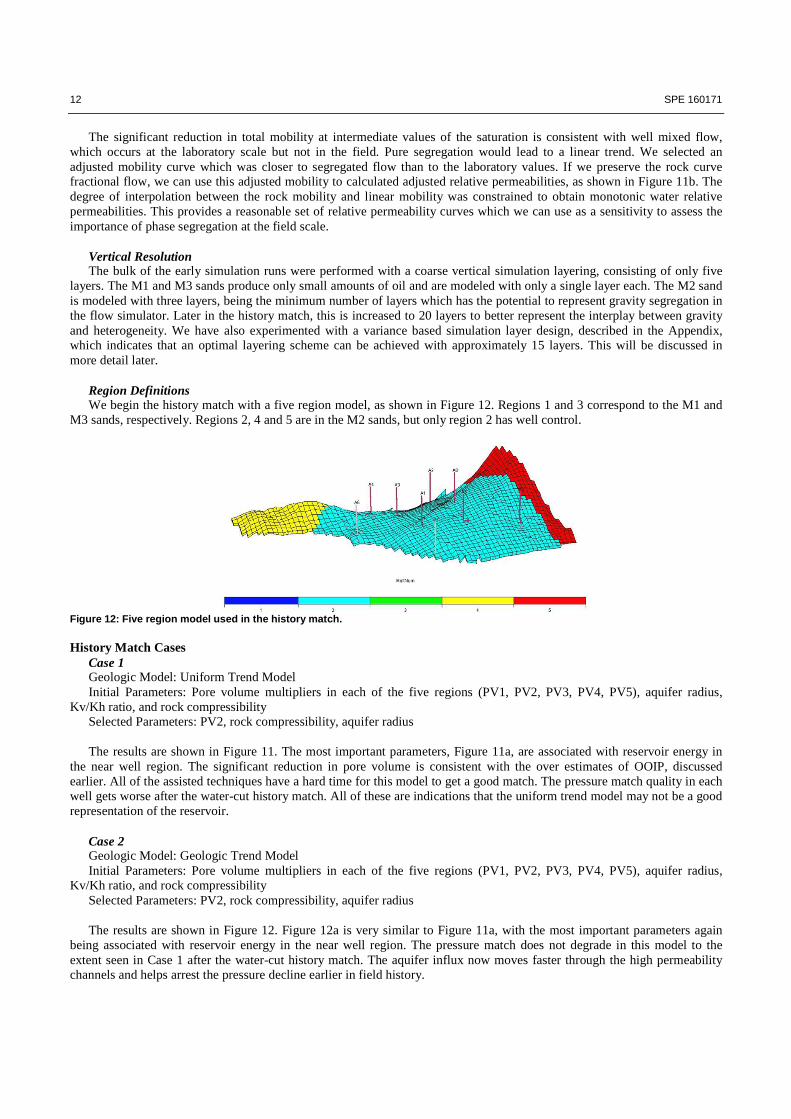
Region Definitions We begin the history match with a five region model, as shown in Figure 12. Regions 1 and 3 correspond to the M1 and

M3 sands, respectively. Regions 2, 4 and 5 are in the M2 sands, but only region 2 has well control.

Figure 12: Five region model used in the history match.

History Match Cases

Case 1 Geologic Model: Uniform Trend Model Initial Parameters: Pore volume multipliers in each of the five regions (PV1, PV2, PV3, PV4, PV5), aquifer radius,

Kv/Kh ratio, and rock compressibility Selected Parameters: PV2, rock compressibility, aquifer radius The results are shown in Figure 11. The most important parameters, Figure 11a, are associated with reservoir energy in

the near well region. The significant reduction in pore volume is consistent with the over estimates of OOIP, discussed earlier. All of the assisted techniques have a hard time for this model to get a good match. The pressure match quality in each well gets worse after the water-cut history match. All of these are indications that the uniform trend model may not be a good representation of the reservoir.

Case 2 Geologic Model: Geologic Trend Model Initial Parameters: Pore volume multipliers in each of the five regions (PV1, PV2, PV3, PV4, PV5), aquifer radius,

Kv/Kh ratio, and rock compressibility Selected Parameters: PV2, rock compressibility, aquifer radius The results are shown in Figure 12. Figure 12a is very similar to Figure 11a, with the most important parameters again

being associated with reservoir energy in the near well region. The pressure match does not degrade in this model to the extent seen in Case 1 after the water-cut history match. The aquifer influx now moves faster through the high permeability channels and helps arrest the pressure decline earlier in field history.

SPE 160171 13

Figure 11: Tornado plot and results of the history match for Case 1 (Uniform Geologic Trend) Historical data is shown as points. The black and red curves represent the match obtained after the pressure history match. The green and blue curves represent the modified match after the water-cut match.

Figure 12: Tornado plot and results of the history match for Case 2 (Geologic Trend) Historical data is shown as points. The black and red curves represent the match obtained after the pressure history match. The green and blue curves represent the modified match after the water-cut match.

Case 3 Geologic Model: Seismic Trend Model Initial Parameters: Pore volume multipliers in each of the five regions (PV1, PV2, PV3, PV4, PV5), aquifer radius,

Kv/Kh ratio, and rock compressibility Selected Parameters: PV2, rock compressibility, aquifer radius The results are almost identical to those of Case 2, Figure 12, and are not shown, although there is an incremental

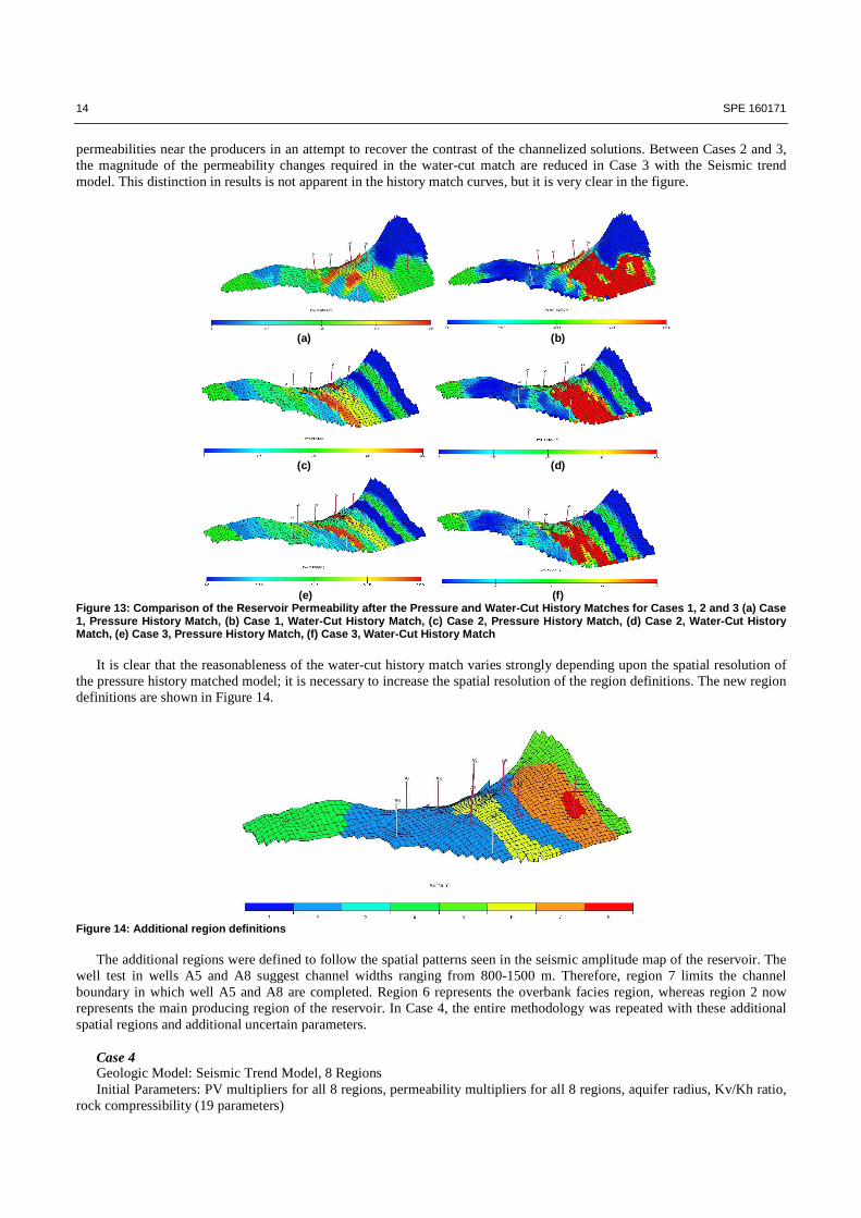
improvement in the pressure history match. At this point we have completed the history match for all three of the initial geologic models, and are about to begin the first of our “outer loop” iterations as we revisit the initial models. However, before revising the starting point it is very informative to contrast the performance of the AHM techniques for these three cases, given the very different initial geologic descriptions. Figure 13 shows the reservoir permeability at the conclusion of the pressure and water-cut history matches for each of the three cases. The streamline-based water-cut history matches are the most informative in the performance of the AHM calculations. Contrasting Figures 13b, 13c, and 13e, it becomes clear that the magnitude of the changes, and their reasonableness, are strongly dependent upon the starting models. For Case 1, and some extent Case 2, the contrast between the channel and non-channel sands is completely lost, and the changes are very large. In detail in Case 1, the streamline techniques have needed to increase the overall sand permeabilities but decrease the

14 SPE 160171

permeabilities near the producers in an attempt to recover the contrast of the channelized solutions. Between Cases 2 and 3, the magnitude of the permeability changes required in the water-cut match are reduced in Case 3 with the Seismic trend model. This distinction in results is not apparent in the history match curves, but it is very clear in the figure.

(a) (b)

(c) (d)

(e) (f)

Figure 13: Comparison of the Reservoir Permeability after the Pressure and Water-Cut History Matches for Cases 1, 2 and 3 (a) Case 1, Pressure History Match, (b) Case 1, Water-Cut History Match, (c) Case 2, Pressure History Match, (d) Case 2, Water-Cut History Match, (e) Case 3, Pressure History Match, (f) Case 3, Water-Cut History Match

It is clear that the reasonableness of the water-cut history match varies strongly depending upon the spatial resolution of

the pressure history matched model; it is necessary to increase the spatial resolution of the region definitions. The new region definitions are shown in Figure 14.

Figure 14: Additional region definitions

The additional regions were defined to follow the spatial patterns seen in the seismic amplitude map of the reservoir. The

well test in wells A5 and A8 suggest channel widths ranging from 800-1500 m. Therefore, region 7 limits the channel boundary in which well A5 and A8 are completed. Region 6 represents the overbank facies region, whereas region 2 now represents the main producing region of the reservoir. In Case 4, the entire methodology was repeated with these additional spatial regions and additional uncertain parameters.

Case 4 Geologic Model: Seismic Trend Model, 8 Regions Initial Parameters: PV multipliers for all 8 regions, permeability multipliers for all 8 regions, aquifer radius, Kv/Kh ratio,

rock compressibility (19 parameters)

SPE 160171 15

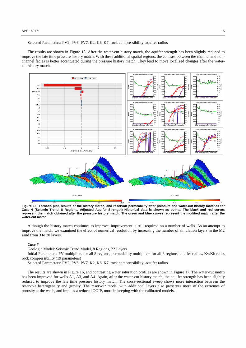
Selected Parameters: PV2, PV6, PV7, K2, K6, K7, rock compressibility, aquifer radius The results are shown in Figure 15. After the water-cut history match, the aquifer strength has been slightly reduced to

improve the late time pressure history match. With these additional spatial regions, the contrast between the channel and non-channel facies is better accentuated during the pressure history match. They lead to move localized changes after the water-cut history match.

11/02 04/04 08/05 01/07 05/08 10/090

1000

2000

3000

4000

5000

6000

7000

8000

(PS

IA)

0

0.1

0.2

0.3

0.4

0.5

0.6

0.7

0.8

0.9

1.0

Water C

ut

A7 WBHPH WBP9 WWCTH WWCT

11/02 04/04 08/05 01/07 05/08 10/090

1000

2000

3000

4000

5000

6000

7000

8000

(PS

IA)

0

0.1

0.2

0.3

0.4

0.5

0.6

0.7

0.8

0.9

1.0

Water C

ut

A6 WBHPH WBP9 WWCTH WWCT

11/02 04/04 08/05 01/07 05/08 10/090

1000

2000

3000

4000

5000

6000

7000

8000

(PS

IA)

0

0.1

0.2

0.3

0.4

0.5

0.6

0.7

0.8

0.9

1.0

Water C

ut

A9 WBHPH WBP9 WWCTH WWCT

11/02 04/04 08/05 01/07 05/08 10/090

1000

2000

3000

4000

5000

6000

7000

8000

(PS

IA)

0

0.1

0.2

0.3

0.4

0.5

0.6

0.7

0.8

0.9

1.0

Water C

ut

A8 WBHPH WBP9 WWCTH WWCT

11/02 04/04 08/05 01/07 05/08 10/090

1000

2000

3000

4000

5000

6000

7000

8000

(PS

IA)

0

0.1

0.2

0.3

0.4

0.5

0.6

0.7

0.8

0.9

1.0

Water C

ut

A5 WBHPH WBP9 WWCTH WWCT

11/02 04/04 08/05 01/07 05/08 10/090

1000

2000

3000

4000

5000

6000

7000

8000

(PS

IA)

0

0.1

0.2

0.3

0.4

0.5

0.6

0.7

0.8

0.9

1.0

Water C

ut

A4 WBHPH WBP9 WWCTH WWCT

11/02 04/04 08/05 01/07 05/08 10/090

1000

2000

3000

4000

5000

6000

7000

8000

(PS

IA)

0

0.1

0.2

0.3

0.4

0.5

0.6

0.7

0.8

0.9

1.0

Water C

ut

A3 WBHPH WBP9 WWCTH WWCT

11/02 04/04 08/05 01/07 05/08 10/090

1000

2000

3000

4000

5000

6000

7000

8000

(PS

IA)

0

0.1

0.2

0.3

0.4

0.5

0.6

0.7

0.8

0.9

1.0

Water C

ut

A2 WBHPH WBP9 WWCTH WWCT

11/02 04/04 08/05 01/07 05/08 10/090

1000

2000

3000

4000

5000

6000

7000

8000

(PS

IA)

0

0.1

0.2

0.3

0.4

0.5

0.6

0.7

0.8

0.9

1.0

Water C

ut

A1 WBHPH WBP9 WWCTH WWCT

Figure 15: Tornado plot, results of the history match, and reservoir permeability after pressure and water-cut history matches for Case 4 (Seismic Trend, 8 Regions, Adjusted Aquifer Strength) Historical data is shown as points. The black and red curves represent the match obtained after the pressure history match. The green and blue curves represent the modified match after the water-cut match.

Although the history match continues to improve, improvement is still required on a number of wells. As an attempt to

improve the match, we examined the effect of numerical resolution by increasing the number of simulation layers in the M2 sand from 3 to 20 layers.

Case 5 Geologic Model: Seismic Trend Model, 8 Regions, 22 Layers Initial Parameters: PV multipliers for all 8 regions, permeability multipliers for all 8 regions, aquifer radius, Kv/Kh ratio,

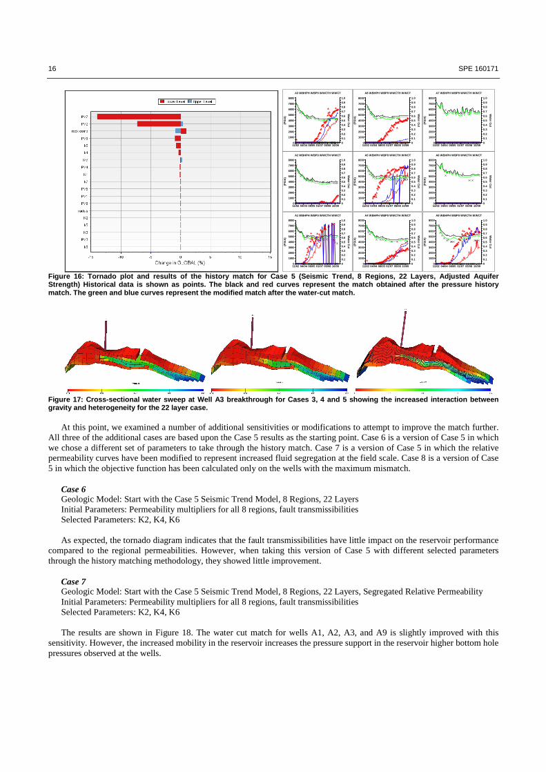
rock compressibility (19 parameters) Selected Parameters: PV2, PV6, PV7, K2, K6, K7, rock compressibility, aquifer radius The results are shown in Figure 16, and contrasting water saturation profiles are shown in Figure 17. The water-cut match

has been improved for wells A1, A3, and A4. Again, after the water-cut history match, the aquifer strength has been slightly reduced to improve the late time pressure history match. The cross-sectional sweep shows more interaction between the reservoir heterogeneity and gravity. The reservoir model with additional layers also preserves more of the extremes of porosity at the wells, and implies a reduced OOIP, more in keeping with the calibrated models.

16 SPE 160171

11/02 04/04 08/05 01/07 05/08 10/090

1000

2000

3000

4000

5000

6000

7000

8000

(PS

IA)

0

0.1

0.2

0.3

0.4

0.5

0.6

0.7

0.8

0.9

1.0

Water C

ut

A7 WBHPH WBP9 WWCTH WWCT

11/02 04/04 08/05 01/07 05/08 10/090

1000

2000

3000

4000

5000

6000

7000

8000

(PS

IA)

0

0.1

0.2

0.3

0.4

0.5

0.6

0.7

0.8

0.9

1.0

Water C

ut

A6 WBHPH WBP9 WWCTH WWCT

11/02 04/04 08/05 01/07 05/08 10/090

1000

2000

3000

4000

5000

6000

7000

8000

(PS

IA)

0

0.1

0.2

0.3

0.4

0.5

0.6

0.7

0.8

0.9

1.0

Water C

ut

A9 WBHPH WBP9 WWCTH WWCT

11/02 04/04 08/05 01/07 05/08 10/090

1000

2000

3000

4000

5000

6000

7000

8000

(PS

IA)

0

0.1

0.2

0.3

0.4

0.5

0.6

0.7

0.8

0.9

1.0

Water C

ut

A8 WBHPH WBP9 WWCTH WWCT

11/02 04/04 08/05 01/07 05/08 10/090

1000

2000

3000

4000

5000

6000

7000

8000

(PS

IA)

0

0.1

0.2

0.3

0.4

0.5

0.6

0.7

0.8

0.9

1.0

Water C

ut

A5 WBHPH WBP9 WWCTH WWCT

11/02 04/04 08/05 01/07 05/08 10/090

1000

2000

3000

4000

5000

6000

7000

8000

(PS

IA)

0

0.1

0.2

0.3

0.4

0.5

0.6

0.7

0.8

0.9

1.0

Water C

ut

A4 WBHPH WBP9 WWCTH WWCT

11/02 04/04 08/05 01/07 05/08 10/090

1000

2000

3000

4000

5000

6000

7000

8000

(PS

IA)

0

0.1

0.2

0.3

0.4

0.5

0.6

0.7

0.8

0.9

1.0

Water C

ut

A3 WBHPH WBP9 WWCTH WWCT

11/02 04/04 08/05 01/07 05/08 10/090

1000

2000

3000

4000

5000

6000

7000

8000

(PS

IA)

0

0.1

0.2

0.3

0.4

0.5

0.6

0.7

0.8

0.9

1.0

Water C

ut

A2 WBHPH WBP9 WWCTH WWCT

11/02 04/04 08/05 01/07 05/08 10/090

1000

2000

3000

4000

5000

6000

7000

8000

(PS

IA)

0

0.1

0.2

0.3

0.4

0.5

0.6

0.7

0.8

0.9

1.0

Water C

ut

A1 WBHPH WBP9 WWCTH WWCT

Figure 16: Tornado plot and results of the history match for Case 5 (Seismic Trend, 8 Regions, 22 Layers, Adjusted Aquifer Strength) Historical data is shown as points. The black and red curves represent the match obtained after the pressure history match. The green and blue curves represent the modified match after the water-cut match.

Figure 17: Cross-sectional water sweep at Well A3 breakthrough for Cases 3, 4 and 5 showing the increased interaction between gravity and heterogeneity for the 22 layer case.

At this point, we examined a number of additional sensitivities or modifications to attempt to improve the match further.

All three of the additional cases are based upon the Case 5 results as the starting point. Case 6 is a version of Case 5 in which we chose a different set of parameters to take through the history match. Case 7 is a version of Case 5 in which the relative permeability curves have been modified to represent increased fluid segregation at the field scale. Case 8 is a version of Case 5 in which the objective function has been calculated only on the wells with the maximum mismatch.

Case 6 Geologic Model: Start with the Case 5 Seismic Trend Model, 8 Regions, 22 Layers Initial Parameters: Permeability multipliers for all 8 regions, fault transmissibilities Selected Parameters: K2, K4, K6 As expected, the tornado diagram indicates that the fault transmissibilities have little impact on the reservoir performance

compared to the regional permeabilities. However, when taking this version of Case 5 with different selected parameters through the history matching methodology, they showed little improvement.

Case 7 Geologic Model: Start with the Case 5 Seismic Trend Model, 8 Regions, 22 Layers, Segregated Relative Permeability Initial Parameters: Permeability multipliers for all 8 regions, fault transmissibilities Selected Parameters: K2, K4, K6 The results are shown in Figure 18. The water cut match for wells A1, A2, A3, and A9 is slightly improved with this

sensitivity. However, the increased mobility in the reservoir increases the pressure support in the reservoir higher bottom hole pressures observed at the wells.

SPE 160171 17

11/02 04/04 08/05 01/07 05/08 10/090

1000

2000

3000

4000

5000

6000

7000

8000

(PS

IA)

0

0.1

0.2

0.3

0.4

0.5

0.6

0.7

0.8

0.9

1.0

Water C

ut

A7 WBHPH WBP9 WWCTH WWCT

11/02 04/04 08/05 01/07 05/08 10/090

1000

2000

3000

4000

5000

6000

7000

8000

(PS

IA)

0

0.1

0.2

0.3

0.4

0.5

0.6

0.7

0.8

0.9

1.0

Water C

ut

A6 WBHPH WBP9 WWCTH WWCT

11/02 04/04 08/05 01/07 05/08 10/090

1000

2000

3000

4000

5000

6000

7000

8000

(PS

IA)

0

0.1

0.2

0.3

0.4

0.5

0.6

0.7

0.8

0.9

1.0

Water C

ut

A9 WBHPH WBP9 WWCTH WWCT

11/02 04/04 08/05 01/07 05/08 10/090

1000

2000

3000

4000

5000

6000

7000

8000

(PS

IA)

0

0.1

0.2

0.3

0.4

0.5

0.6

0.7

0.8

0.9

1.0

Water C

ut

A8 WBHPH WBP9 WWCTH WWCT

11/02 04/04 08/05 01/07 05/08 10/090

1000

2000

3000

4000

5000

6000

7000

8000

(PS

IA)

0

0.1

0.2

0.3

0.4

0.5

0.6

0.7

0.8

0.9

1.0

Water C

ut

A5 WBHPH WBP9 WWCTH WWCT

11/02 04/04 08/05 01/07 05/08 10/090

1000

2000

3000

4000

5000

6000

7000

8000

(PS

IA)

0

0.1

0.2

0.3

0.4

0.5

0.6

0.7

0.8

0.9

1.0

Water C

ut

A4 WBHPH WBP9 WWCTH WWCT

11/02 04/04 08/05 01/07 05/08 10/090

1000

2000

3000

4000

5000

6000

7000

8000

(PS

IA)

0

0.1

0.2

0.3

0.4

0.5

0.6

0.7

0.8

0.9

1.0

Water C

ut

A3 WBHPH WBP9 WWCTH WWCT

11/02 04/04 08/05 01/07 05/08 10/090

1000

2000

3000

4000

5000

6000

7000

8000

(PS

IA)

0

0.1

0.2

0.3

0.4

0.5

0.6

0.7

0.8

0.9

1.0

Water C

ut

A2 WBHPH WBP9 WWCTH WWCT

11/02 04/04 08/05 01/07 05/08 10/090

1000

2000

3000

4000

5000

6000

7000

8000

(PS

IA)

0

0.1

0.2

0.3

0.4

0.5

0.6

0.7

0.8

0.9

1.0

Water C

ut

A1 WBHPH WBP9 WWCTH WWCT

Figure 18: Results of the history match for Case 7. Historical data is shown as points. The black and red curves represent the match obtained after the pressure history match. The green and blue curves represent the modified match after the water-cut match.

The well with the remaining worst history match is A8. In Case 8 we repeat Case 7, but now with the objective function

only calculated for that well. Case 8 Geologic Model: Case 7 Model (Objective function calculated on Well A8 only) Initial Parameters: PV multipliers for all 8 regions, permeability multipliers for all 8 regions, aquifer radius, Kv/Kh ratio,

rock compressibility (19 parameters) Selected Parameters: PV2, PV3, PV7, K2, aquifer radius

11/02 04/04 08/05 01/07 05/08 10/090

1000

2000

3000

4000

5000

6000

7000

8000

(PS

IA)

0

0.1

0.2

0.3

0.4

0.5

0.6

0.7

0.8

0.9

1.0

Water C

ut

A7 WBHPH WBP9 WWCTH WWCT

11/02 04/04 08/05 01/07 05/08 10/090

1000

2000

3000

4000

5000

6000

7000

8000

(PS

IA)

0

0.1

0.2

0.3

0.4

0.5

0.6

0.7

0.8

0.9

1.0

Water C

ut

A6 WBHPH WBP9 WWCTH WWCT

11/02 04/04 08/05 01/07 05/08 10/090

1000

2000

3000

4000

5000

6000

7000

8000

(PS

IA)

0

0.1

0.2

0.3

0.4

0.5

0.6

0.7

0.8

0.9

1.0

Water C

ut

A9 WBHPH WBP9 WWCTH WWCT

11/02 04/04 08/05 01/07 05/08 10/090

1000

2000

3000

4000

5000

6000

7000

8000

(PS

IA)

0

0.1

0.2

0.3

0.4

0.5

0.6

0.7

0.8

0.9

1.0

Water C

ut

A8 WBHPH WBP9 WWCTH WWCT

11/02 04/04 08/05 01/07 05/08 10/090

1000

2000

3000

4000

5000

6000

7000

8000

(PS

IA)

0

0.1

0.2

0.3

0.4

0.5

0.6

0.7

0.8

0.9

1.0

Water C

ut

A5 WBHPH WBP9 WWCTH WWCT

11/02 04/04 08/05 01/07 05/08 10/090

1000

2000

3000

4000

5000

6000

7000

8000

(PS

IA)

0

0.1

0.2

0.3

0.4

0.5

0.6

0.7

0.8

0.9

1.0

Water C

ut

A4 WBHPH WBP9 WWCTH WWCT

11/02 04/04 08/05 01/07 05/08 10/090

1000

2000

3000

4000

5000

6000

7000

8000

(PS

IA)

0

0.1

0.2

0.3

0.4

0.5

0.6

0.7

0.8

0.9

1.0

Water C

ut

A3 WBHPH WBP9 WWCTH WWCT

11/02 04/04 08/05 01/07 05/08 10/090

1000

2000

3000

4000

5000

6000

7000

8000

(PS

IA)

0

0.1

0.2

0.3

0.4

0.5

0.6

0.7

0.8

0.9

1.0

Water C

ut

A2 WBHPH WBP9 WWCTH WWCT

11/02 04/04 08/05 01/07 05/08 10/090

1000

2000

3000

4000

5000

6000

7000

8000

(PS

IA)

0

0.1

0.2

0.3

0.4

0.5

0.6

0.7

0.8

0.9

1.0

Water C

ut

A1 WBHPH WBP9 WWCTH WWCT

Figure 19: Tornado plot for the Well A8 water-cut and results of the history match for Case 8 (Adjusted Aquifer Strength), Historical data is shown as points. The black and red curves represent the match obtained after the pressure history match. The green and blue curves represent the modified match after the water-cut match.

18 SPE 160171

Figure 20: Goodness of fit for pressure and water-cut for all of the cases studied

The results are shown in Figure 19. The tornado diagram for the water-cut match of Well A8 includes the PV3 parameter

which is not included within the higher ranked parameters for the overall objective function. Again, the aquifer strength has been reduced to improve the pressure history match at late times.

Further sensitivities have been performed, but there has not been an overall improvement. Although the water-cut or pressure history match may be improved for individual wells, it is at the expense of other wells. A summary of the pressure and water-cut goodness of fit for all of the cases studied is shown in Figure 20.

Reservoir Description

A number of the parameters determined during the history matching process are summarized in Tables 2-4. The pore volume distribution indicates that as more regions are defined in the M2 sands, the pore volume fraction is more

effectively segregated between the channel and non-channel regions. The permeability follows this same trend, with better reservoir quality within the channels.

Regions Region 2 Region 6 Region 7

Cases Parameter Before

Pressure Match

After Pressure Match

Before Pressure Match

After Pressure Match

Before Pressure Match

After Pressure Match

Case 1 PV 0.5 0.24 NA NA NA NA Case 2 PV 0.5 0.26 NA NA NA NA Case 3 PV 0.5 0.25 NA NA NA NA

Case 4 PV 0.8 0.35 0.5 0.14 0.8 0.2

Perm 1 1.2 1 0.2 1 1

Case 5 PV 0.6 0.41 0.4 0.2 0.5 0.2

Perm 1 1 0.5 0.3 1 1

Case 8 PV 0.5 0.42 0.3 0.2 0.3 0.2

Perm 1 1 0.3 0.3 1 1 Table 2: Pore Volume and Permeability Multipliers for the different cases

The rock compressibility governs the initial decline in reservoir pressure. I observed in each case the trend in the initial

reservoir pressure drop is better matched by using rock compressibility of 3E-5 1/psia. In the late time, aquifer influx becomes the major drive mechanism. However, high aquifer strength contributed to greater mismatch in the late time pressure trend. So, ultimately there is a trade-off between the quality of pressure history match and the water cut history match. The aquifer strength had to be reduced to maintain the energy balance.

SPE 160171 19

Cases

Aquifer Radius, ft Before

Pressure Match

After Pressure Match

Case 1 800 905 Case 2 800 925 Case 3 800 895 Case 4 800 1065 Case 5 800 856 Case 8 800 896

Table 3: Aquifer strength for different cases

Cases

Rock Compressibility, 1/psia Before

Pressure Match

After Pressure Match

Case 1 13.88E-5 3E-5

Case 2 13.88E-5 3E-5

Case 3 13.88E-5 3E-5

Case 4 13.88E-5 3E-5

Case 5 13.88E-5 3E-5

Case 8 13.88E-5 3E-5 Table 4: Rock compressibility for different cases

Simulation Layer Design

As an additional technical study, we have reviewed the question of vertical resolution required to adequately represent the interplay of gravity, heterogeneity, and cross-sectional sweep. To this end we have made two changes in the reservoir model construction. First, the geologic model is constructed at close to log resolution, which for this reservoir, implies 420 layers. Now essentially no averaging is done in moving from log scale to the blocked well scale of the geologic model. Second, we have used the techniques described in the Appendix to derive an optimal reservoir simulation layering scheme from this high resolution geologic model. Interestingly, the resulting resolution is comparable to that used in the history matching study, with 15 layers in the M2 sand.

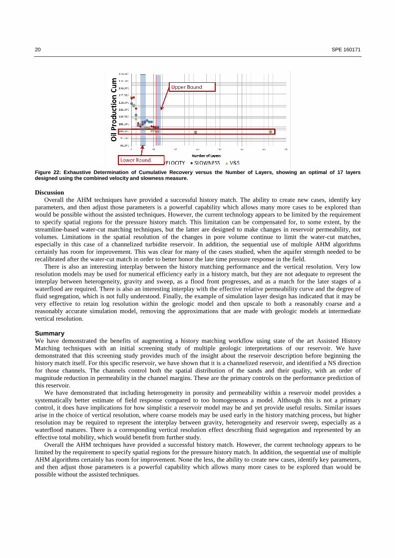
The optimal layering design is one for which any additional layer coarsening will remove so much heterogeneity from the model that sweep and recovery begins to increase dramatically. The statistical error measure that appears to work best for many cases is a combination of velocity and slowness. More details are in the Appendix, but the results are shown in Figures 21 and 22. In these two figures, an exhaustive selection of layering schemes is evaluated using flow simulation. In both figures, the results verify that the optimal layering scheme, obtained by a non-simulation statistical measure, provides a good estimate of the optimal number of layers. With this degree of coarsening, the simulation run time is reduced by a factor of 20-40 compared to flow simulation on the original geologic layer resolution.

Figure 21: Cumulative Field Oil Production as a function of the number of simulation layers. Black is the reference case. Blue has more than 33 layers. Red has 10-17 layers. Green has less than 10 layers. The optimal range is given by the red cases.

20 SPE 160171

Figure 22: Exhaustive Determination of Cumulative Recovery versus the Number of Layers, showing an optimal of 17 layers designed using the combined velocity and slowness measure.

Discussion

Overall the AHM techniques have provided a successful history match. The ability to create new cases, identify key parameters, and then adjust those parameters is a powerful capability which allows many more cases to be explored than would be possible without the assisted techniques. However, the current technology appears to be limited by the requirement to specify spatial regions for the pressure history match. This limitation can be compensated for, to some extent, by the streamline-based water-cut matching techniques, but the latter are designed to make changes in reservoir permeability, not volumes. Limitations in the spatial resolution of the changes in pore volume continue to limit the water-cut matches, especially in this case of a channelized turbidite reservoir. In addition, the sequential use of multiple AHM algorithms certainly has room for improvement. This was clear for many of the cases studied, when the aquifer strength needed to be recalibrated after the water-cut match in order to better honor the late time pressure response in the field.

There is also an interesting interplay between the history matching performance and the vertical resolution. Very low resolution models may be used for numerical efficiency early in a history match, but they are not adequate to represent the interplay between heterogeneity, gravity and sweep, as a flood front progresses, and as a match for the later stages of a waterflood are required. There is also an interesting interplay with the effective relative permeability curve and the degree of fluid segregation, which is not fully understood. Finally, the example of simulation layer design has indicated that it may be very effective to retain log resolution within the geologic model and then upscale to both a reasonably coarse and a reasonably accurate simulation model, removing the approximations that are made with geologic models at intermediate vertical resolution. Summary We have demonstrated the benefits of augmenting a history matching workflow using state of the art Assisted History Matching techniques with an initial screening study of multiple geologic interpretations of our reservoir. We have demonstrated that this screening study provides much of the insight about the reservoir description before beginning the history match itself. For this specific reservoir, we have shown that it is a channelized reservoir, and identified a NS direction for those channels. The channels control both the spatial distribution of the sands and their quality, with an order of magnitude reduction in permeability in the channel margins. These are the primary controls on the performance prediction of this reservoir.

We have demonstrated that including heterogeneity in porosity and permeability within a reservoir model provides a systematically better estimate of field response compared to too homogeneous a model. Although this is not a primary control, it does have implications for how simplistic a reservoir model may be and yet provide useful results. Similar issues arise in the choice of vertical resolution, where coarse models may be used early in the history matching process, but higher resolution may be required to represent the interplay between gravity, heterogeneity and reservoir sweep, especially as a waterflood matures. There is a corresponding vertical resolution effect describing fluid segregation and represented by an effective total mobility, which would benefit from further study.

Overall the AHM techniques have provided a successful history match. However, the current technology appears to be limited by the requirement to specify spatial regions for the pressure history match. In addition, the sequential use of multiple AHM algorithms certainly has room for improvement. None the less, the ability to create new cases, identify key parameters, and then adjust those parameters is a powerful capability which allows many more cases to be explored than would be possible without the assisted techniques.

SPE 160171 21

Acknowledgements The authors acknowledge the financial support of the sponsors of the Model Calibration and Efficient Reservoir Imaging (MCERI) JIP at Texas A&M University. We thank a major oil and gas producer for access to the field data, and we thank Dr. Duane McVay for many fruitful discussions. Nomenclature i,j,k Cell indices

ijkn Net rock volume in a cell

ijkφ Cell porosity

Cijkφ Coarsened cell porosity

AHM Assisted History Matching GTTI Generalized Travel Time Inversion Kh Horizontal permeability, mD Kv Vertical permeability, mD

ijkK Cell permeability (horizontal), mD

CijkK Coarsened cell permeability (horizontal), mD

NTG Net to Gross ratio References Back, T. 1996. Evolutionary Algorithms in Theory and Practice, Chap. 2, 68-73. New York: Oxford Univ. Press. Back, T., Hammel, U., and Schwefel, H.P. 1997. Evolutionary Computation: Comments on the History and Current State. Evolutionary

Computation, IEEE Transactions 1 (1): 3-17. Bhark, E., Datta-Gupta, A. and Jafarpour, B. 2011. History Matching with a Multiscale Parameterization Based on Grid Connectivity and

Adaptive to Prior Information. Paper SPE 147372 presented at the Annual Technical Conference and Exhibition, Denver, Colorado, USA, 30 October-2 November, doi 10.2118/147372-MS.

Box, G.E.P. and Draper, N.R. 1987. Empirical Model-Building and Response Surfaces: Wiley. Cheng, H., Dehghani, K. and Billiter, T. 2008. A Structured Approach for Probabilistic-Assisted History Matching Using Evolutionary

Algorithms: Tengiz Field Applications. Paper SPE 116212 presented at the Annual Technical Conference and Exhibition, Denver, Colorado, USA, 21-24 September, doi 10.2118/116212-MS.

Datta-Gupta, Akhil, editor, 2009. History Matching and Conditioning Geologic Models to Production Data. SPE preprint series, Society of Petroleum Engineers.

ECLIPSE 2011. http://www.slb.com/services/software/reseng/eclipse.aspx Eide, A.L., Holden, L., Reiso, E., and Aanonsen, S.I. 1994. Automatic History Matching by use of Response Surfaces and Experimental

Design. In the Proceedings of the 4th European Conference on the Mathematics of Oil Recovery, Roros, Norway, 7–10 June. GeoGraphix 2012. http://www.lmkr.com/geographix/ He, Z., Yoon, S. and Datta-Gupta, A. 2002. Streamline-Based Production Data Integration with Gravity and Changing Field Conditions.

SPE Journal 7(4) December 2002: 423-436, doi 10.2118/81208-PA. Hosseini, S.A., and Kelkar M., 2010. Analytical Upgridding Method To Preserve Dynamic Flow Behavior. SPEREE 13(3) June 2010: 473-

484, doi 10.2118/116113-PA. King, M.J., Burn, K.S., Wang, P et.al. 2006. Optimal Coarsening of 3D Reservoir Models for Flow Simulation. SPEREE 9(4) August

2006: 317-334, doi 10.2118/95759-PA. Luo, Y. and Schuster, G.T. 1991. Wave-Equation Traveltime Inversion. Geophysics 56, No. 5, 645. MCERI 2011. http://www.pe.tamu.edu/mceri/ MEPO 2012. http://www.sptgroup.com/en/Products/MEPO/ Milliken, W.J., Emanuel, A.S., and Chakravarty, A. 2001. Applications of 3D Streamline Simulation to Assist History Matching. SPEREE

4(6) December 2001: 502-508, doi 10.2118/74712-PA. Moulds, T.P., Trussell, P., Haseldonckx, S.A. et.al. 2005. Magnus Field: Reservoir Management in a Mature Field Combining Waterflood,

EOR, and New Area Developments. Paper SPE 96292 presented at Offshore Europe, Aberdeen, United Kingdom, 6-9 September, doi 10.2118/96292-MS.

Rey, A., Ballin, P., Chick V. et.al. 2009. Assisted History Matching in an Offshore Turbidite Reservoir With Active Reservoir Management. Paper SPE 124950 presented at the Annual Technical Conference and Exhibition, New Orleans, Louisiana, USA, 4-7 October, doi 10.2118/124950-MS.

RMS 2012. http://www2.emersonprocess.com/en-US/brands/roxar/reservoirmanagement/ Schulze-Riegert, R.W., Haase, O., and Nekrassov, R.K. 2003. Combined Global and Local Optimization Techniques Applied to History

Matching. Paper SPE 79668 presented at the SPE Reservoir Simulation Symposium, Houston, Texas, 3-5 February, doi 10.2118/79668-MS.

Vasco, D.W., Yoon, S., and Datta-Gupta, A. 1999. Integrating Dynamic Data into High-Resolution Reservoir Models Using Streamline-Based Analytic Sensitivity Coefficients. SPE Journal 4(4) December 1999: 389-399 doi 10.2118/59253-PA.

White, C.D. and Royer, S.A. 2003. Experimental Design as a Framework for Reservoir Studies. Paper SPE 79676 presented at the SPE Reservoir Simulation Symposium, Houston, Texas, 3-5 February, doi 10.2118/79676-MS.

22 SPE 160171

White, C.D., Willis, B.J., Narayanan, K. et.al. 2001. Identifying and Estimating Significant Geologic Parameters with Experimental Design. SPE Journal 6(3) September 2001: 311-324, doi 10.2118/74140-PA.

Williams, G.J.J., Mansfield, M., MacDonald, D.G. and Bush, M.D. 2004. Top-Down Reservoir Modeling. Paper SPE 89974 presented at the Annual Technical Conference and Exhibition, Houston, Texas, USA, 26-29 September, doi 10.2118/89974-MS.

Williams, M.A., Keating, J.F. and Barghouty, M.F. 1998. The Stratigraphic Method: A Structured Approach to History Matching Complex Simulation Models. SPEREE 1(2) April 1998: 169-176, doi 10.2118/38014-PA.

Wu, Z. and Datta-Gupta, A. 2002. Rapid History Matching Using a Generalized Travel-Time Inversion Method. SPE Journal 7(2) June 2002: 113-122, doi 10.2118/78359-PA.

Xie, J., Mondal A., Efendiev Y., Mallick B., and Datta-Gupta, A. 2010. History Matching Channelized Reservoirs Using Reversible Jump Markov Chain Monte Carlo Methods. Paper SPE 129685 presented at the SPE Improved Oil Recovery Symposium, Tulsa, Oklahoma, USA, 24-28 April, doi 10.2118/129685-MS.

Appendix: Layer Grouping Analysis This discussion is an extension of the earlier works of King et.al. 2006 and Hosseini and Kelkar 2010. Consider a 3D geologic model with each cell characterized by a porosity and a (horizontal) permeability. If we consider a horizontal viscous dominated flow, then we may create any of several measures to understand the error introduced as we coarsen this model to one with fewer layers. If we impose a pressure gradient across a column of the model, then we may calculate the interstitial

fluid velocity in each cell of that column. It is proportional to ijkijkK φ . Similarly, we may calculate the transit time across

this same cell, otherwise known as the slowness. It is proportional to ijkijk Kφ . If we now group layers and replace the

porosity and permeability in each cell by their coarsened, net rock volume weighted arithmetic averages, then we can use the variation in velocity or slowness as error measures.

∑

−⋅=

ijkCijk

Cijk

ijk

ijkijkV

KKnW

2

φφ ∑

−⋅=

ijkCijk

Cijk

ijk

ijkijkS KK

nW

2φφ

The first of these measures is most sensitive to high permeability streaks and does the best job of assessing the error in breakthrough times. The second of these measures provides the best estimate of error in time of flight, which controls the overall saturation distribution. It provides the best overall estimate of the error in multiphase flow resulting from layer coarsening. Hosseini and Kelkar suggested combining the two errors to provide increased sensitivity to breakthrough time to

the slowness error measure: SVVS WWW ⋅= . Now, let’s consider a sequential calculation beginning with a high resolution

geologic model. The initial error vanishes since the coarsened properties are identical to the initial properties. If we now consider all possible pairwise layer coarsenings, then we can calculate the coarsened values for porosity and permeability for each layer pair, and the corresponding error measure. Select the layer coarsening which minimizes the increase in the error. Repeat until a single layer is obtained. The shape of the curve will exhibit a bias-variance cross over. The optimal layering scheme is obtained from this curve by identification of the number of layers beyond which the error increases rapidly. The sequence of layering schemes, and the identification of a specific optimal choice, is dependent upon the choice of error measure. In the current study we have shown that the combined Velocity+Slowness error works better than either of the other individual errors in the simulation layering design and prediction of the optimal number of layers.