SPE 156163

Integrated Dynamic Flow Analysis to Characterize an Unconventional Reservoir in Argentina: The Loma La Lata Case Matías Fernandez Badessich and Vicente Berrios, YPF

Copyright 2012, Society of Petroleum Engineers This paper was prepared for presentation at the SPE Annual Technical Conference and Exhibition held in San Antonio, Texas, USA, 8-10 October 2012. This paper was selected for presentation by an SPE program committee following review of information contained in an abstract submitted by the author(s). Contents of the paper have not been reviewed by the Society of Petroleum Engineers and are subject to correction by the author(s). The material does not necessarily reflect any position of the Society of Petroleum Engineers, its officers, or members. Electronic reproduction, distribution, or storage of any part of this paper without the written consent of the Society of Petroleum Engineers is prohibited. Permission to reproduce in print is restricted to an abstract of not more than 300 words; illustrations may not be copied. The abstract must contain conspicuous acknowledgment of SPE copyright.

Abstract In November 2010 YPF brought online the very first shale oil well in Argentina in the northern area of Loma La Lata field after successfully fracturing the Vaca Muerta formation, the main source rock in the Neuquen basin. Initial choked productivity exceeded 250 bopd of high quality oil from an average depth of 9,500 ft. Since then, YPF has pioneered a new era of production from unconventional reservoirs in Argentina with many more wells coming onstream.

As it is well known, production forecasting and reserves estimation in this kind of reservoirs is fraught with challenges and pitfalls. Many methods have been applied so far; these range from very simple decline curve analysis to highly elaborate reservoir simulation models.

In order to understand and monitor the production behaviour of the YPF wells, several reservoir and production analysis techniques have been applied such as pressure transient analysis, rate transient analysis, interpretation of available DFITs and time-lapsed production logging measurements.

In this paper we present what YPF has implemented as a robust workflow for analyzing dynamic data that captures the physics of the flow process, explains the observed data and provides a method for forecasting reserves for a range of assumed in-place volumes. Introduction The Vaca Muerta shale play is lithologically associated with a Late Jurassic mixed shale (calcareous and silicoclastic) that was developed along the northwestern part of the Argentinean Patagonia, in the Neuquen Basin (Figure 1). The Vaca Muerta Formation is a lithostratigraphic unit that can be easily recognized in outcrops as “black bituminous marls”. The composing sedimentary architecture corresponds to a distal facies of a mixed carbonate sequence developed between the Jurassic Tithonan and Valanginian ages. This extremely prolific, world-class source rock was deposited during the Tithonian (Late Jurassic) transgression that took place in the Neuquen Basin that rapidly flooded the underlying eolian and fluvial units of the Tordillo Formation (Kimmeridgian). This transgression marks the maximum basin expansion of the marine environment than extended for about 30,000 km2. Locally, the shales and marls deposited under external marine platform conditions behind an active volcanic back-arc, developed organic-rich facies from anoxic conditions, reaching a TOC content that varies between 1 to 8% with spikes of 12%. These rocks contain high-quality, amorphous algal organic material, mainly I/II kerogen type; the thickness ranges from 25 m in the proximal areas, all the way up to 450 m at the basin center. This is coincident with the present depth distribution, ranging from less than 1000 m at the basin margin down to 4000 m near the basin center. Due to this wide aereal distribution, variable thickness and overburden, Vaca Muerta has produced all kind of hydrocarbons: low GOR liquid hydrocarbons, volatile oils, gas/condensate and dry gas progressively through time; today, three distinct hydrocarbon generation windows can be geographically identified throughout the basin as shown in Figure 2. According to log and core analysis, the matrix porosity of the Vaca Muerta shale varies from 4 to 14% with an average of 9% while matrix permeabilities span from hundreds of nanodarcies to tens of microdarcies. The presence of natural fractures has also been recognized; they play a very important role in initial well rates.

2 SPE 156163

Since November 2010 when the very first shale oil well was opened to production, YPF has brought onstream 27 vertical wells and 3 horizontal wells with remarkable success.

Most of the wells have required massive hydraulic fractures to achieve commercial rates. Typically, four fracture stages were performed in the vertical wells while ten stages were executed in the (roughly) 1000 m horizontals At the time of writing this paper, YPF has already carried out more than a hundred frac jobs with a very small percentage of screen outs. Additionally, some wells (approximately 30%) have penetrated sweet spots where the upper Vaca Muerta seems to be naturally fractured so these wells produce without any stimulation at all. As a matter of fact, once these high pressure/high productivity zones are tapped, drilling operations can hardly continue because wells are very difficult to control in this condition. As a consequence, the BHA is retrieved and the well is completed open hole.

Due to the fact that this was a new play coming on production in Argentina and the need to characterize it appropriately to optimize its development, a comprehensive surveillance program was designed to accomplish this mission. Data acquisition plan The data gathering strategy consisted of capturing the right information at the right time. This collection plan involved acquiring the following static and dynamic data:

! Core and log data ! Geomechanical studies ! DFITs in key wells ! Microseismic monitoring ! Wellhead pressures and temperatures during production ! Downhole pressures and temperatures via retrievable downhole gauges ! Time-lapsed production logging surveys ! Full set of oil, gas and water chemical analysis ! Tracer analysis

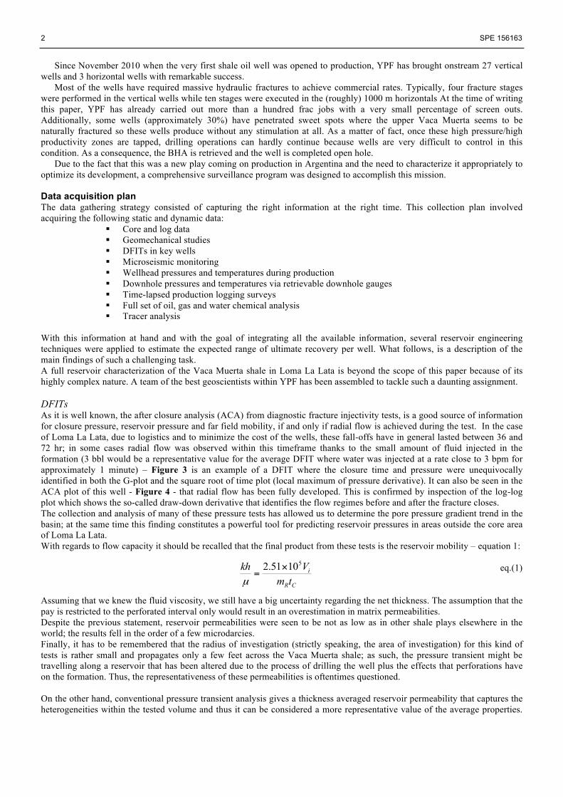
With this information at hand and with the goal of integrating all the available information, several reservoir engineering techniques were applied to estimate the expected range of ultimate recovery per well. What follows, is a description of the main findings of such a challenging task. A full reservoir characterization of the Vaca Muerta shale in Loma La Lata is beyond the scope of this paper because of its highly complex nature. A team of the best geoscientists within YPF has been assembled to tackle such a daunting assignment. DFITs As it is well known, the after closure analysis (ACA) from diagnostic fracture injectivity tests, is a good source of information for closure pressure, reservoir pressure and far field mobility, if and only if radial flow is achieved during the test. In the case of Loma La Lata, due to logistics and to minimize the cost of the wells, these fall-offs have in general lasted between 36 and 72 hr; in some cases radial flow was observed within this timeframe thanks to the small amount of fluid injected in the formation (3 bbl would be a representative value for the average DFIT where water was injected at a rate close to 3 bpm for approximately 1 minute) – Figure 3 is an example of a DFIT where the closure time and pressure were unequivocally identified in both the G-plot and the square root of time plot (local maximum of pressure derivative). It can also be seen in the ACA plot of this well - Figure 4 - that radial flow has been fully developed. This is confirmed by inspection of the log-log plot which shows the so-called draw-down derivative that identifies the flow regimes before and after the fracture closes. The collection and analysis of many of these pressure tests has allowed us to determine the pore pressure gradient trend in the basin; at the same time this finding constitutes a powerful tool for predicting reservoir pressures in areas outside the core area of Loma La Lata. With regards to flow capacity it should be recalled that the final product from these tests is the reservoir mobility – equation 1: eq.(1)

Assuming that we knew the fluid viscosity, we still have a big uncertainty regarding the net thickness. The assumption that the pay is restricted to the perforated interval only would result in an overestimation in matrix permeabilities. Despite the previous statement, reservoir permeabilities were seen to be not as low as in other shale plays elsewhere in the world; the results fell in the order of a few microdarcies. Finally, it has to be remembered that the radius of investigation (strictly speaking, the area of investigation) for this kind of tests is rather small and propagates only a few feet across the Vaca Muerta shale; as such, the pressure transient might be travelling along a reservoir that has been altered due to the process of drilling the well plus the effects that perforations have on the formation. Thus, the representativeness of these permeabilities is oftentimes questioned. On the other hand, conventional pressure transient analysis gives a thickness averaged reservoir permeability that captures the heterogeneities within the tested volume and thus it can be considered a more representative value of the average properties.

CR

i

tmVkh 51051.2 !

=µ

SPE 156163 3

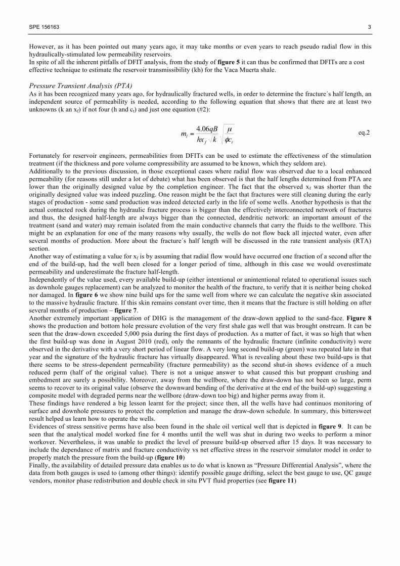
However, as it has been pointed out many years ago, it may take months or even years to reach pseudo radial flow in this hydraulically-stimulated low permeability reservoirs. In spite of all the inherent pitfalls of DFIT analysis, from the study of figure 5 it can thus be confirmed that DFITs are a cost effective technique to estimate the reservoir transmissibility (kh) for the Vaca Muerta shale. Pressure Transient Analysis (PTA) As it has been recognized many years ago, for hydraulically fractured wells, in order to determine the fracture´s half length, an independent source of permeability is needed, according to the following equation that shows that there are at least two unknowns (k an xf) if not four (h and ct) and just one equation (#2):

eq.2

Fortunately for reservoir engineers, permeabilities from DFITs can be used to estimate the effectiveness of the stimulation treatment (if the thickness and pore volume compressibility are assumed to be known, which they seldom are). Additionally to the previous discussion, in those exceptional cases where radial flow was observed due to a local enhanced permeability (for reasons still under a lot of debate) what has been observed is that the half lengths determined from PTA are lower than the originally designed value by the completion engineer. The fact that the observed xf was shorter than the originally designed value was indeed puzzling. One reason might be the fact that fractures were still cleaning during the early stages of production - some sand production was indeed detected early in the life of some wells. Another hypothesis is that the actual contacted rock during the hydraulic fracture process is bigger than the effectively interconnected network of fractures and thus, the designed half-length are always bigger than the connected, dendritic network: an important amount of the treatment (sand and water) may remain isolated from the main conductive channels that carry the fluids to the wellbore. This might be an explanation for one of the many reasons why usually, the wells do not flow back all injected water, even after several months of production. More about the fracture´s half length will be discussed in the rate transient analysis (RTA) section. Another way of estimating a value for xf is by assuming that radial flow would have occurred one fraction of a second after the end of the build-up, had the well been closed for a longer period of time, although in this case we would overestimate permeability and underestimate the fracture half-length. Independently of the value used, every available build-up (either intentional or unintentional related to operational issues such as downhole gauges replacement) can be analyzed to monitor the health of the fracture, to verify that it is neither being choked nor damaged. In figure 6 we show nine build ups for the same well from where we can calculate the negative skin associated to the massive hydraulic fracture. If this skin remains constant over time, then it means that the fracture is still holding on after several months of production – figure 7. Another extremely important application of DHG is the management of the draw-down applied to the sand-face. Figure 8 shows the production and bottom hole pressure evolution of the very first shale gas well that was brought onstream. It can be seen that the draw-down exceeded 5,000 psia during the first days of production. As a matter of fact, it was so high that when the first build-up was done in August 2010 (red), only the remnants of the hydraulic fracture (infinite conductivity) were observed in the derivative with a very short period of linear flow. A very long second build-up (green) was repeated late in that year and the signature of the hydraulic fracture has virtually disappeared. What is revealing about these two build-ups is that there seems to be stress-dependent permeability (fracture permeability) as the second shut-in shows evidence of a much reduced perm (half of the original value). There is not a unique answer to what caused this but proppant crushing and embedment are surely a possibility. Moreover, away from the wellbore, where the draw-down has not been so large, perm seems to recover to its original value (observe the downward bending of the derivative at the end of the build-up) suggesting a composite model with degraded perms near the wellbore (draw-down too big) and higher perms away from it. These findings have rendered a big lesson learnt for the project; since then, all the wells have had continuos monitoring of surface and downhole pressures to protect the completion and manage the draw-down schedule. In summary, this bittersweet result helped us learn how to operate the wells. Evidences of stress sensitive perms have also been found in the shale oil vertical well that is depicted in figure 9. It can be seen that the analytical model worked fine for 4 months until the well was shut in during two weeks to perform a minor workover. Nevertheless, it was unable to predict the level of pressure build-up observed after 15 days. It was necessary to include the dependance of matrix and fracture conductivity vs net effective stress in the reservoir simulator model in order to properly match the pressure from the build-up (figure 10) Finally, the availability of detailed pressure data enables us to do what is known as “Pressure Differential Analysis”, where the data from both gauges is used to (among other things): identify possible gauge drifting, select the best gauge to use, QC gauge vendors, monitor phase redistribution and double check in situ PVT fluid properties (see figure 11)

tfl ckhx

qBm!µ06.4

=

4 SPE 156163

Rate Transient Analysis (RTA) This technique has evolved so much over the past few years that now it represents one of the most powerful means that reservoir engineers have at hand to understand and forecast tight and shale wells; it should be acknowledged though that it encompasses a significant degree of ambiguity and non-uniqueness. It is not the intention of this paper to describe the RTA technique; the literature abounds with excellent material on this subject. YPF has adopted the following workflow for analyzing rate/pressure data:

! QA/QC the data to remove the outliers and to isolate the reservoir signal from operational related noises, such as rapidly changing parameters during the flowback and open and shut events that create additional transients that mask the linear flow response

! Determine the linear flow parameter (and confirm the existence of linear flow) through specialized analysis with the square root of time plot

! Estimate the absolute minimum stimulated reservoir volume (SRV) through flowing material balance (FMB) ! Generate an analytical model that history matches the performance ! Run forecasts and sensitivities to the main variables affecting the ultimate recovery of the well

QA/QC: This is a strongly recommended step prior to any quantitative analysis. What it has to be captured is the underlying reservoir signature that might be shadowed by erratic pressure/rate points and by changing wellbore conditions such as paraffin deposits (observed in these wells), liquid loading, scale deposition, etc. Additionally, these effects should not be confused with apparent boundary dominated flow that would erroneously imply that the SRV is extremely small. Specialized analysis: Plotting !P/q (rate normalized pressures) vs SQRT should render a straight line (in linear flow regime) from whose slope, the product can be extracted. Also, this plot is very useful to diagnose losses in productivity. The gas well mentioned previously that had those two build-ups was also the focus of this analysis (Figure 12). Three very clear production stages can be identified here:

1. Flow back through casing 2. Linear flow once the 2 3/8 tubing was installed 3. Linear flow again but with a much more reduced productivity that manifests itself as a change in slope

It should be recalled that the slope of this plot for a gas well is (equation #3): eq.3 So if the the product of goes down in the denominator, then the slope ml increases accordingly. As in the case of PTA, there is no way to detach the flowing area (the product of fracture thickness times the fracture half length) from the permeability without an independent measurement of the other variable. Nonetheless, determining this linear flow parameter, has allowed us to create a ranking among the wells that should throw some light to understand how the hydraulic fractures can be optimized; the bigger the value, the better the group [h.xf.k1/2] becomes for a vertical well. Furthermore, the intercept of this plot can be associated to an apparent skin; the bigger the value of the intercept, the higher the skin is and the more relevant becomes the understanding of the underlying causes. In figure 13 an example of the first horizontal oil well is shown from where both and S´ were estimated. It can be observed that the well is slightly damaged. Lastly, as every vertical well has a PLT log, the producing thickness can be estimated rather well. In such a circumstance the problem can be reduced to just assuming the value of effective permeability and analyzing the resulting fracture half length (and then listening to the completion engineer complains!). It is a sort of trial and error exercise that helps to bracket the value of the effective perm. For the case of a vertical well, we get the results shown in the following table:

Table 1. Sensitivities to permeability and resulting fracture half lengths xf.k^1/2 = 25

Permeability Permeability Fracture half length Completion engineer´s comments md µd ft 0.0500 50 112 “I should be fired!” 0.0100 10 250 “Maybe” 0.0050 5 354 “This is the fracture I designed” 0.0020 2 559 “I should get a bonus” 0.0010 1 791 “I wish I were that good”

kA

kA

kA

kA

tl ckA

Tm!µ11262

=

SPE 156163 5

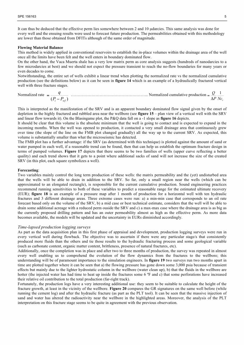
It can thus be deduced that the effective perm lies somewhere between 2 and 10 µdarcies. This same analysis was done for every well and the ensuing results were used to forecast future production. The permeabilities obtained with this methodology are lower than those obtained from DFITs although of the same order of magnitude. Flowing Material Balance This method is widely applied in conventional reservoirs to establish the in-place volumes within the drainage area of the well once all the limits have been felt and the well enters in boundary dominated flow. On the other hand, the Vaca Muerta shale has a very low matrix perm as core analysis suggests (hundreds of nanodarcies to a few microdarcies at best) and we should not expect the pressure transient to reach the no-flow boundaries for many years or even decades to come. Notwithstanding, the entire set of wells exhibit a linear trend when plotting the normalized rate vs the normalized cumulative production (see the definitions below) as it can be seen in figure 14 which is an example of a hydraulically fractured vertical well with three fracture stages. Normalized rate ………………………………………………... Normalized cumulative production This is interpreted as the manifestation of the SRV and is an apparent boundary dominated flow signal given by the onset of depletion in the highly fractured and rubbled area near the wellbore (see figure 15 – plan view of a vertical well with the SRV and linear flow towards it). On the Blasingame plot, the P&Q data fall on a -1 slope as figure 16 depicts. It should be clear that this volume is the absolute minimum that the well is going to contact and is expected to expand in the incoming months. When the well was opened to production, it contacted a very small drainage area that continuously grew over time (the slope of the line on the FMB plot changed gradually) all the way up to the current SRV. As expected, this volume is substantially smaller than what the microseismic has detected. The FMB plot has a further advantage: if the SRV (as determined with this technique) is plotted against the amount of sand or water pumped in each well, if a reasonable trend can be found, then that can help us establish the optimum fracture design in terms of pumped volumes. Figure 17 depicts that there seems to be two families of wells (upper curve reflecting a better quality) and each trend shows that it gets to a point where additional sacks of sand will not increase the size of the created SRV (in this plot, each square symbolizes a well). Forecasting: Two variables mainly control the long term production of these wells: the matrix permeability and the (yet) undisturbed area that the wells will be able to drain in addition to the SRV. So far, only a small region near the wells (which can be approximated to an elongated rectangle), is responsible for the current cumulative production. Sound engineering practices recommend running sensitivities to both of these variables to predict a reasonable range for the estimated ultimate recovery (EUR); figure 18 is an example of a pressure map after 1 month of production for a horizontal well with ten hydraulic fractures and 3 different drainage areas. Three extreme cases were run: a) a min-min case that corresponds to an oil rate forecast based only on the volume of the SRV, b) a mid case or best technical estimate, considers that the well will be able to drain some additional acreage with a reduced perm ouside the SRV and c) a max-max case where the drainage area is as big as the currently proposed drilling pattern and has an outer permeability almost as high as the effective perm. As more data becomes available, the models will be updated and the uncertainty in EURs diminished accordingly. Time-lapsed production logging surveys As part as the data acquisition plan in this first phase of appraisal and development, production logging surveys were run in every vertical well during flowback. The objective was to ascertain if there were any particular stage/s that consistently produced more fluids than the others and tie those results to the hydraulic fracturing process and some geological variable (such as carbonate content, organic matter content, brittleness, presence of natural fractures, etc). Additionally, once the completion was in place and after two to three months of production, the survey was repeated in almost every well enabling us to comprehend the evolution of the flow dynamics from the fractures to the wellbore; this understanding will be of paramount importance to the simulation engineers. In figure 19 two surveys run two months apart in time are plotted together where it can be seen that a) the flowing pressure has gone down some 3,000 psia because of transient effects but mainly due to the lighter hydrostatic column in the wellbore (water clean up), b) that the fluids in the wellbore are hotter (the injected water has had time to heat up inside the fractures some 6 ºF and c) that some perforations have increased their relative oil contribution to the total production (far-right track). Fortunately, the production logs have a very interesting additional use: they seem to be suitable to calculate the height of the fracture growth, at least in the vicinity of the wellbore. Figure 20 compares the GR signatures on the same well before (while running the cement log) and after the hydraulic fracture (as part as the PLT tool). It can be seen that the massive injection of sand and water has altered the radioactivity near the wellbore in the highlighted areas. Moreover, the analysis of the PLT interpretation on this fracture stage seems to be quite in agreement with the previous observation.

)( wfi PPq!

=tNcP

Q 1!

=

6 SPE 156163

Fluid analysis A thorough fluid sampling program was implemented to help us understand not only the in-situ fluid characteristics but also the dynamic behavior of the system of fractures + reservoir. There exists a general trend in oil properties with a general west-east trend as depicted in figure 21. Additionally, the picture 22 shows the gradation in colors of the crude oil as we move in a westward direction; obviously, the gas content of these fluids increases to the west towards the center of the basin. The oil wells that fell near the zone where the oil becomes volatile have some phase behavior issues such as an increasing GOR and relative permeability effects. Not only there is a presence of an areal distribution of fluids but also there exists a vertical trend too. It has been observed that wells completed in zones where Vaca Muerta is deeper, they produce slightly lighter oil. This observation has been substantiated by the analysis in conjunction of PLTs and oil gravities. As said before, PLTs are run at different times and most of them show that initially the shallower fractures tend to produce most of the oil with the water being segregated at the bottom; later, the reiteration of this log indicates that the deepest fractures begin to give oil to the wellbore concurrently with an increase in API vs time as figure 23 shows for one particular well of the project. To characterize the produced water, aliquots were taken on a regular basis to monitor the evolution of its composition. The water salinity increased very rapidly in a few weeks from just a few thousand parts per million (ppm of chlorides) up to more than 100,000 ppm for some wells. This visibly has a direct influence on the economics of the project due to the need to treat the water before it can be reutilized or disposed of (the salinity of the frac water should be lower than 2,000 ppm to avoid the use of scale and corrosion inhibitors). Hydraulic fracturing in the Vaca Muerta shale Design of the fracturing treatment

As of the time of writing this paper, the number of wells drilled and stimulated with MHF from 2010 to Q1-2012 in the Vaca Muerta shale adds up to 31 verticals and 4 horizontals. Initial attempts to successfully stimulate the Vaca Muerta formation have proven to be challenging at the least.

The first hydraulically fractured well used only slickwater at very low proppant concentrations and less than 5% of linear gel. Then, the design evolved - as did the learning curve - and now a combination of slickwater, linear and crosslinked gel is at the order of the day. This solution was seeked in order to accomplish two critical goals: a) to maximize the fracture complexity and b) to optimize the fracture conductivity without compromising the life of the proppant. Slickwater still accounts for more than 35% of the total fluid pumped. The injection rate ranges from 24 to 76 bbl/min (depending on the number of clusters treated together), most of the treatment being at 70 bpm with 4 clusters. The amount proppant per stage averages around 477,000 lbs with a typical maximum final concentration of 6 ppa. The proppant of choice is a combination of 50/120, 40/80, 30/50 and 20/40 mesh. The proppant type is mostly ceramics and coated sand due to the high ISIP values. Average treating pressure is around 7,200 psi with a range of 2,800 to 10,300 psi. The number of stages per well varies from 1 to 4 for vertical wells and from 7 to 11 for horizontals. Figures 24 and 25 summarize the completion strategy. Geomechanics and microseismic In the area of Loma La Lata, the direction of maximum stress has been determined from image logs and borehole breakouts to have a WNW-ESE direction and thus, the horizontals are being drilled orthogonal to this direction so that they can be fractured parallel to this maximum stress – figure 26 very clearly shows the borehole breakouts in a vertical well in addition to the microseismic events in two verticals located to the north and south of the monitor well. Additionally, this can also be seen in figure 27 which shows in plan view a 1000 meter horizontal well drilled parallel to the minimum stress (Sh min) together with the seismic events that depict the extent to which the hydraulic fractures span. In this location, two horizontal wells separated only 80 meters in the vertical direction were selected to shoot microseimic: the shallower well had a horizontal array of eigth geophones with 30 meters between each sensor device that was pulled out of the hole as each fracture stage was being performed in the deepest well (figure 28). The results were highly revealing and showed that the fractures tend to grow with a spherical aspect ratio because of the existence of a situation of similar stresses due to the high pore pressures. Moreover, there might be chances for these two wells to interfere in the future, although this is yet to be confirmed by an in place tracer program were 7 out of 10 stages were inoculated. Pressure monitoring during fracturing operations Of the more than one hundred hydraulic fracture jobs, one interesting case will be shown here that stresses the value of data integration across the different disciplines. This is a vertical well that produces dry gas where four fracture stages were done and one in particular (stage #3) is responsible for most of the gas production as the PLT shows in figure 29. The analysis of the step rate down tests undoubtedly reveals that this behavior was to be expected as the stage #3 had the fastest pace of pressure fall-off (red curve), indicative of an enhanced permeability probably due to the presence of a naturally fractured network. (figure 30)

SPE 156163 7

Conclusions The Vaca Muerta shale is an extraordinarily attractive shale play that so far has shown very encouraging results. Most of

the activity has been focused in the Loma La Lata block but YPF is rapidly expanding its exploration and appraisal effort all across the Neuquen basin.

In order to better understand and characterize the behavior of this shale play, YPF has embarked in an intensive campaign to capture and integrate as much data as possible. Most of the information shown in this paper comes from the engineering realm (reservoir, production and completion) although a parallel effort is currently being pursued by YPF´s geoscientists.

A lot of effort should be directed to estimate more accurately the effective fracture height, its half length and the possible degradation of the fracture´s conductivity with net confining stress.

The integrated work that has been presented here aims, among other things, at optimizing the fracture design to maximize the well´s productivity while minimizing completion costs.

A combination of RTA techniques and reservoir simulation are the recommended tools to attain an understanding of the shale physics deep enough to guarantee that YPF is in the right track to soundly develop the Vaca Muerta shale.

As it happens in every emerging shale play around the world there are still some uncertainties that only more data, time and effort will eventually unravel. Nevertheless, the presented workflow has allowed YPF to narrow down some of these uncertainties and has provided us with a tool to reasonably forecast oil and gas production.

Needless to say, the success of this venture will strongly depend on a multidisciplinary team approach.

8 SPE 156163

Acknowledgements We wish to thank Mr Hernán Maretto and Dr. Tomás Zapata for their help with the geological description. Mr Emmanuel d´Huteau and Mr. Daniel García for the valuable interchange of ideas on DFITs and hydraulic fractures, Iván Lanusse, Malena Rodriguez, Nicolás Kotlar, Mariano Suarez, and Damián Hryb for their help with the pictures and very special thanks to Jose Gil and his field operations team for the invaluable work they are doing at supervising and acquiring a big part of the the data presented in this paper. We would also like to thank Dr. Carlos Glandt for his support, to all those who consider the reservoir limit test a priceless reservoir engineering tool and YPF for its permission to publish this paper.

Nomenclature

A = flow area (net thickness x fracture half length) ct = total compressibility ! = porosity FMB = flowing material balance DFIT = diagnostic fracture injectivity test h = net thickness, ft k = permeability, md mR = slope of the plot of pressure vs the time function (F) MHF = massive hydraulic fracture N = stock tank oil in place Pi = initial reservoir pressure Pwf = flowing pressure q = flow rate Q = cumulative oil production S´ = apparent skin factor Shmin = minimum horizontal stress SRV = stimulated rock volume tC = closure time, minutes Vi = injected volume, bbl µ = viscosity, cp xf = fracture half length tLDf = end of linear flow in dimensionless time

References Agarwal, R., Carter, D. and Pollock, C.: “Evaluation and Performance Prediction of Low-Permeability Gas Wells

Stimulated by Massive Hydraulic Fracturing”, paper SPE 6838 presented at the SPE-AIME 52nd Annual Fall Technical Conference and Exhibition, Denver, CO, 9-12 October 1977

Anderson, D., Nobakht, M., Moghadam, S. and Mattar, L.: “Analysis of Production Data from Fractured Shale Gas Wells” paper SPE 131787, presented at the SPE Unconventional Gas Conference held in Pittsburgh, PA, 23-25 February 2010

Anderson, D. and Liang, P.: “Quantifying Uncertainty in Rate Transient Analysis for Unconventional Gas Reservoirs”, paper SPE 145088 presented at the SPE North American Unconventional Gas Conference and Exhibition held in The Woodlands, TX, 14-16 June 2011

Barree, R, Barree, V. and Craig, D.: “Holistic Fracture Diagnostics: Consistent Interpretation of Prefrac Injection Tests Using Multiple Analysis Methods”, paper SPE 107877, presented at the 2007 SPE Rocky Mountain Oil & Gas Technology Symposium, Denver, CO, 16-18 April 2007.

Clarkson, C and Pedersen, P.: “Tight Oil Production Analysis: Adaptation of Existing Rate-Transient Analysis Techniques”, paper CSUG/SPE 137352 presented at the Canadian Unconventional Resources & International Petroleum Conference held in Calgary, Alberta, 19-21 October 2010.

Clarkson, C., Jensen, J. and Blasingame, T.: “Reservoir Engineering for Unconventional Gas Reservoirs: What Do We Have to Consider?”, paper SPE 145080 presented at the SPE North American Unconventional Gas Conference and Exhibition held in The Woodlands, TX, 14-16 June 2011

Cliff, W., Boertje, A. and Fjaere, O.: “Use of Pressure Gauge Differentials in Well Test Quality Control and Well Performance Evaluation”, paper SPE 24288 presented at the SPE European Petroleum Computer Conference held in Stavenger, Norway, 25-27 May 1992

d´Hutteau, E.: “Design and implementation of Mini-Frac Tests”, YPF´s internal training program Kappa Engineering: “The Analysis of Dynamic Data in Shale Gas Reservoirs – Part I” December 2010

SPE 156163 9

Kappa Engineering: “The Analysis of Dynamic Data in Shale Gas Reservoirs – Part II” Lancaster, D., McKetta, S., Hill, R., Guidry, F. and Jochen, J., SPE 24884 presented at the 67th Annual Technical

Conference and Exhibition of the Society of Petroleum Engineers held in Washington, DC, October 4-7, 1992 Liang, P., Mattar, L and Moghadam, S.: Analyzing Variable Rate/Pressure Data in Transient Linear Flow in

Unconventional Gas Reservoirs”, paper CSUG/SPE 149472 presented at the Canadian Unconventional Resources Conference held in Calgary, 15-17 November 2011

Nolte, K., Maniere, J. and Owens, K. “After-Closure Analysis of Calibration Tests”, paper SPE 38676 presented at the 1997 SPE Annual Technical Conference and Exhibition held in San Antonio, TX, 5-8 October 1997

Stotts, G., Anderson, D. and Mattar, L.: “Evaluating and Developing Tight Gas Reserves – Best Practices”, paper SPE 108183 presented at the SPE 2007 Rocky Mountain Oil and Gas Technology Symposium held in Denver, CO, 16-18 April 2007

Strickland, R., Purvis, D. and Blasingame, T.: “Practical Aspects of Reserves Determinations for Shale Gas”, paper SPE 144357 presented at the SPE North American Unconventional Gas Conference and Exhibition held in The Woodlands, TX, 14-16 June 2011

Thompson, J.M., Nobakht, M. and Anderson, D.: “Modeling Well Performance Data From Overpressured Shale Gas Reservoirs”, paper CSUG/SPE 137755 presented at the Canadian Unconventional Resources & International Petroleum Conference held in Calgary, Alberta, 19-21 October 2010.

Thompson, J.M., M´Angha, V., Anderson, D.: “Advancements in Shale Gas Production Forecasting – A Marcellus Case Study”, paper SPE 144436 presented at the SPE Americas Unconventional Gas Conference and Exhibition held in The Woodlands, TX, 14-16 June 2011

Figure 1 – Loma La Lata location

Figure 2 – Hydrocarbon generation window

LOMA LA LATA BLOCK

10 SPE 156163

Closure time and pressure identified by the departure of the straight line that goes through the origin

Figure 3 – Closure time and closure pressure as determined from a DFIT for a Loma La Lata well

1E-4 1E-3 0.01 0.1 1Square Linear Flow (FL^2)

100

1000

!"#$%&'(#$)**($+$#,-./-%#0%&12-$#3((4#-52/(6(.

!"! #$%&'()%* + ,-)./%!"! #)0/%* + ,-)$%&'()1 23&2$&3/#34$(456

0 10 20 30 40 50 60 7

G-function

0

100

200

300

400

500

Pres

sure

[psi

]

!"#$%&'(!)(* "#$%&'* +(!)(* "#$%&'

Figure 4 – Pseudo radial flow that allows the estimation of far field mobility

0.01 0.1 1 10 100

100

1000

10000

!"#$%&$'()*+, -.$/0, -.$/12)34562)34/72)34/18-(9:$/8-(9:$5&;<(450

Infinite conductivity fracture signature

Figure 5 – Simulation of the time required to reach radial flow in the Vaca Muerta shale

Figure 6 – Nine build-ups in the same well show a hydraulically fractured well with NO radial flow

Figure 7 – Skin evolution over time: as the skin is relatively constant, it is interpreted that the hydraulic fracture remains open

Time, hr

Pressure, psi

Time

SPE 156163 11

0.01 0.1 1 10 100 1000 10000

1E+7

1E+8

1E+9

!"# $%&'&() * $%&'&+,-./0

Figure 8 – Two build-ups done in the same well suggest degradation of the fractures and permeability near the wellbore

100

200

300

400

500

Liqu

id ra

te [S

TB/D

]

4000

8000

12000

16000

Liqu

id v

olum

e [S

TB]

0 400 800 1200 1600 2000 2400 2800 3200 3600 4000 440

Time [hr]

2000

4000

6000

8000

Pre

ssur

e [p

sia]

Figure 9 – History match of a LLL well that shows that a 15-day build-up was not properly matched

Figure 10 – The red curve shows that the numerical simulator required the use of matrix and fracture pressure dependent perms to get a good match

Time, hr

Pseudo Pressure

12 SPE 156163

Figure 11 – An example of the application of pressure differential analysis with the help from down hole gauges

0 5 10 15 20 25 30 35 40 45 50 55 60 65 70 75Time**0.5 [hr**0.5]

0

1E+6

2E+6

3E+6

4E+6

5E+6

6E+6

Gas

pot

entia

l/Gas

rate

[[ps

i2/c

p]/[M

scf/D

]]

Figure 12 – Evidences of productivity losses in a vertical gas well

Figure 13 – Linear flow analysis in a horizontal well to determine apparent skin and kA

´S

Flowback thru casing

Early linear flow

Change in slope due to loss in productivity

Normalized pressure, psi/bpd

SPE 156163 13

0 0.02 0.04 0.06 0.08 0.1 0.12 0.14 0.16 0.18 0.2 0.22 0.24 0.26 0.28

Large liquid volume [MMSTB]

0

0.004

0.008

0.012

0.016

0.02

0.024

Liqu

id ra

te/P

ress

ure

[[m3/

D]/p

sia]

Figure 14 – Flowing material balance to determine the absolute minimum volume connected to the well

Figure 15 – Plan view of an idealized model

1E-4 1E-3 0.01 0.1 1 10 100

0.1

1

10

Figure 16 – The same data as the one in figure 14 but presented in terms of the Blasingame

plot

Figure 17 – SRV as determined with FMB vs #sacks of sand pumped into formation

Figure 18 – Pressure map after 1 month of production using a numerical model for a

horizontal well

14 SPE 156163

''( ) * "

"""

Flowback(8000 psi)

PLT after 2 months(5000 psi)

FRAC #4

FRAC #3

FRAC #2

FRAC #1

, -" . . /-" .0, ( ( 1 2 34 5 ( 6#. 78 9:;;; <;;;#$%%& '()'%*+,-./0111 2111

Flowback(204 ºF)

PLT after 2 mos(210 ºF)

= ">#.3 45$%%& '()'%*67/811 891

= ? @, ( ( 1 2 34 5 ( 6AB 92;; 2C;

Flowback

2nd PLT

! " '$8 (0D#:; 3 <=%%> 8(?8%*!9@A/<B C1

0EF = GH ( ( ) 5 3 I5 ( 6>CJ! 9GK L;

Figure 19 – Time-lapsed PLT surveys that help identify the production evolution from each perforation cluster

Figure 20 – Two gamma ray logs run before and after fracturing suggest the fracture growth near the wellbore. These results agree with the PLT survey

on the right hand of the picture

Figure 21 – areal distribution of crude oil quality in API

Figure 22 – oil samples from Vaca Muerta. Left

bottle is from a gas condensate. The API and the C1 content decreases from left to right

LOMA LA LATA BLOCK

SPE 156163 15

Figure 23 suggests that not all the fractures start producing oil at the same time and also implies that

there exists a vertical gradation of crudes

!"#

"$#

%$#

!"#$%&"'()*!+&',*-./%01/

&'()*+,-./ 0(1.,'23.' 4'(1*23.'

!"#$%#

&$#

!&#

!"#$%&"'()*+",--#(%*./0%120

"'(!$' &'()' *'("' $'(&'

Figure 24 – Summary of fluids and proppant mesh used in the Vaca Muerta shale fractures

Figure 25 – These six charts succinctly capture the main variables of the hydraulic fractures

Figure 26 – Max and min stresses from borehole breakouts. The direction in which the microseismic

events grow agree with SHmax

Figure 27 (left) – Plan view from a horizontal well drilled parallel to Shmin, together with the

microseismic events

16 SPE 156163

North-South lateral view

Figure 28 – Lateral view of both horizontals showing their relative position to the Vaca Muerta shale with the position of the geophones and the microseismic events

from each of the ten stages

2100

2200

2300

! "#$%!

'( ) * """"

Flowmeter, rps

Stage #4

Stage #3

Stage #2

Stage #1

, '-./"$" 0#$%&'("))*) &+"*,+(

Zone rates, m3/d

1 2 $" 3 ( 456 78!+-.&'* ')*

Figure 29 – PLT from a gas vertical well that shows that most of the gas production is coming from fracture #3

Figure 30 – The rate of decline of the fracture #3 in the SRDT was already suggesting that more production was to be expected from this zone