SPE 144618

Geochemical Allocation of Commingled Oil Production or Commingled Gas Production Mark A. McCaffrey, SPE, Weatherford Laboratories; Danielle H. Ohms, SPE, BP Exploration (Alaska) Inc.; Michael Werner, ConocoPhillips Alaska, Inc.; Christopher Stone, SPE, BP Exploration (Alaska) Inc.; David K. Baskin, Brooks A. Patterson, Weatherford Laboratories

Copyright 2011, Society of Petroleum Engineers This paper was prepared for presentation at the SPE Western North American Regional Meeting held in Anchorage, Alaska, USA, 7–11 May 2011. This paper was selected for presentation by an SPE program committee following review of information contained in an abstract submitted by the author(s). Contents of the paper have not been reviewed by the Society of Petroleum Engineers and are subject to correction by the author(s). The material does not necessarily reflect any position of the Society of Petroleum Engineers, its officers, or members. Electronic reproduction, distribution, or storage of any part of this paper without the written consent of the Society of Petroleum Engineers is prohibited. Permission to reproduce in print is restricted to an abstract of not more than 300 words; illustrations may not be copied. The abstract must contain conspicuous acknowledgment of SPE copyright.

Abstract

We have made substantial improvements to the previously published methods for geochemical allocation of commingled oil production and/or commingled gas production. This new method has allowed allocation of commingled production from wells at less than 2-5% of the cost of production logging. Four case studies are shown here. In the first two studies, commingling of the wells was subject to approval of the Alaska Oil and Gas Conservation Commission (AOGCC). Before agreeing to the use of geochemical allocation, the AOGCC required the well operator to perform multi-month trial studies in which the wells were monitored both by geochemical allocation and by production logging. The individuals performing the geochemical allocation were kept blind from the results of the production logging until the studies were completed. Close agreement between the geochemistry-based allocation values and the production-logging-based allocation values resulted in AOGCC approval of continued use of the geochemical method for oil production monitoring of these two wells. Two additional case studies presented here illustrate how geochemical allocation can be used to monitor the effects on production of (1) changes in water injection into nearby wells, and (2) closing or opening perforations within a well. Introduction

Previous methods for using oil composition differences to allocate commingled production from a single well have been detailed in Kaufman et al. (1987 and 1990). Similar methods for allocating the contribution of multiple fields to commingled pipeline production streams are discussed by Hwang et al. (2000). The methods described in those publications relied on using Whole-Oil Gas Chromatography (GC) peak ratios to quantify the contribution of multiple zones to a commingled production stream. In brief, if two zones were being commingled (“Zone A” and “Zone B”), then the respective contributions of Zones A and B to a commingled sample were determined, in those publications, by identifying chemical differences between "end-member" oils (with the end members being a pure sample of oil from Zone A and a pure sample of oil from Zone B). Geochemical parameters (GC peak ratios) reflecting these compositional differences were measured in the end member oils, in various artificial mixtures of the end member oils, and in the commingled oil. The data were then used to mathematically express the composition of the commingled oil in terms of contributions from the respective end member oils. Using this simple mixing model, a single geochemical difference between oils from two sands is sufficient to allocate commingled production from those two units. By using data for several peak ratios, independent solutions to the problem could be derived, allowing the accuracy of the allocation to be assessed. This older approach for geochemical allocation had two drawbacks. The first was that it required analysis of artificial mixtures of the end member oils. This necessity existed because ratios of GC peak heights do not necessarily mix linearly: ratios of peak heights only mix linearly when the same absolute value is present in the denominator of the ratio of the two GC peak heights in all of the end member oils being mixed. For example, if the ratio of the height of GC Peak A and GC Peak B is measured in 3 end member oils, and is found to be 7/2 in “Oil X”, 9/2 in “Oil Y”, and 9/3 in “Oil Z”, then the value for the ratio of Peak A/Peak B will mix linearly between Oil X and Oil Y (since Peak B has a value of 2 in both oils), but will not mix linearly between Oil X and Oil Z (since Peak B has a value of 2 in one oil but 3 in the other oil). Therefore, in the older approach, artificial mixes of end member oils had to be prepared to determine the shape of the calibration curve that defines how a given GC ratio changes as one moves from 100% Oil X to 100% Oil Y.

2 SPE 144618

The second drawback to the older approach was that allocation was limited to 2 or 3 zones. This limitation arose because, for a given GC ratio, two end members when mixed form a mixing curve, and 3 end members when mixed form a mixing surface, but, when more than 3 end members are mixed, there is no simple graphical representation of the mixing from which one could derive a solution. McCaffrey et al. (1996) proposed an alternate approach that was based on GC peak heights and not GC peak height ratios. This approach had the advantages of NOT requiring analysis of artificial mixtures of end member oils (since peak heights always mix linearly) and of also being applicable to any number of mixed zones. The method described here is an advancement on the McCaffrey et al. (1996) approach, and is described in the next section. Methods Allocation of Commingled Oils Dead oil samples (samples collected at the surface at ~ 1 atmosphere pressure) were analyzed by Gas Chromatography (GC) at Weatherford Laboratories (Shenandoah, TX) using an Agilent GC equipped with a 60 m DB-1 Agilent column; the injector was at 275°C, and the heating program was: 35°C (hold 5 minutes), 3°/min. ramp to 320°C (hold for 20 minutes). The carrier gas was helium. GC peak data were processed to calculate the production allocation splits using a proprietary geochemical production allocation software package (OilUnmixerTM, versions 2 through 5, developed by OilTracers LLC, now a part of Weatherford Laboratories). The allocation algorithms in that software are based on the approach described below. If there are no systematic sources of error, then the relationship between a GC peak-height “Y” (measured in the GC trace of a commingled oil) and the GC peak heights “X” of the corresponding peaks in the “m” end-members oils being commingled is given by a linear relationship of the form: Y = β1X1 + β2X2 + ... βmXm. Production allocation is the process of determining the values of β. However, in reality, there are multiple sources of error. For example, there is (1) analytical error in measuring the height of each GC peak, (2) error associated with potential contamination of GC peaks, and (3) error associated with the non-ideality of the samples chosen as end members (for example, when end member oils are taken not from the same well as the commingled oil, but rather from nearby single-zone producing wells that may not be laterally continuous with the commingled well). As a result of the various sources of error, certain GC peaks will do a better job than other peaks at allocating the contributions of each zone to a commingled oil. We cannot know in advance which GC peaks will do the best job, and, in an oil allocation project, many hundreds of different GC peaks are available for use. This problem, therefore, becomes a problem of linear regression. Specifically, given a set of samples containing a value for each independent variable and the corresponding value of the dependent variable, we seek to compute the β values in a relationship of the form: Y = β1X1 + β2X2 + ... βmXm. + eps Where, “eps” represents the error that is not captured by the linear relationship. Linear regression can be used to converge upon a set of β values that minimizes the sum of the square of the errors. For example, as noted by McCaffrey et al. (1996): β = (X'X)-1X'Y is a simple way to derive an estimate of the β vector. From our estimate of the β vector, we are then able to compute the error in each sample point, square that error, and sum it to give S. This value is used to compute the variance of eps as: S/(n-m), where n is the number of peaks and m is the number of end-members. This gives sigma, the standard deviation of eps.

SPE 144618 3

β is not a single number, it is a vector; therefore, its distribution is a joint distribution. As a result, we can again use linear regression to compute the variances in the elements of the β vector from variance of eps. This gives us the standard error in βj. Finally, we can use that value to compute the confidence interval around βj. In numerous un-published studies conducted between 2000 and 2010, we have found that significantly better estimates of the β vector can be derived by techniques such as:

(1) Scaling the raw values for X and Y prior to solving forβ . The issue can be illustrated as follows: Imagine that 4 end member oils are analyzed along with one commingled oil that is a mixture of the 4 end member oils. A table of GC peak heights is then compiled for the 5 oils in this project. In that table, GC “Peak A” has peak heights that range from 5000 to 7000 pA. In contrast, for the same 5 oils, GC “Peak B” has peak heights that range from 200 to 800 pA. Now, assume that all the GC peaks in the table have an uncertainty of 3%. A 3% error on a large GC peak is a larger absolute number than a 3% error on a small GC peak. Therefore, if raw (i.e., un-scaled) GC peak heights are used to solve for β, then the linear regression (which seeks to minimize the absolute error) will seek to fit the “Peak A” data more than the “Peak B” data, even though the “Peak B” data may contain as much information about the source of the oil as do the “Peak A” data. To avoid this preferential treatment of the larger GC peaks, the GC peak height data can first be scaled so as to cause the values for “Peak A” and the values for “Peak B” to cover the same numerical range.

(2) Utilizing information revealed by the structure of the variance within the dataset. Inherent in the allocation approach of McCaffrey et al. (1996) is the assumption that the errors in the allocation are normally distributed about the “true answer”. This assumption can be tested, and where it is found not to be true, that information can be utilized. For example, using a random number generator, one can randomly select hundreds of different subsets of GC peaks from the overall GC peak dataset. One can then independently solve each of these subsets of peaks for β. If, for example, 200 GC peaks are measured in each sample, then a large number of different combinations of just 50 of the 200 GC peaks could be selected, and each of those sets of 50 peaks could be solved for β. If 300 different subsets (of 50 peaks each) were chosen, then that exercise would yield 300 different allocation results for the problem. The 300 allocation results could then be plotted on a histogram, where the x-axis is the % contribution from a given zone, and the y-axis is the number of times that value was derived among the 300 results. If the errors are normally distributed, then the histogram will be bell-shaped. The narrower the bell, the more perfectly the commingled oil can be expressed as a combination of those end member oils. The wider the bell, the, less perfectly the commingled oil can be expressed as a combination of those end member oils. To the extent that the histogram is not bell-shaped (e.g., if the histogram has a single maxima but non-symmetrical tails on either side of that maxima, or, alternatively, if the histogram is multimodal) the peak data set is not ideal. Such a situation reveals the presence of one or more invalid end member oils. The invalid nature of the end members may be due to geological reasons or the presence of contamination in one or more end member oils.

(3) Eliminating from consideration GC peaks with certain specific characteristics. The histogram described in the previous paragraph can allow one to identify which specific GC peaks repeatedly contribute to allocation results that differ substantially from the results implied by the overall dataset (i.e., which peaks consistently show up in the subsets of peaks that yielded the allocation solutions that fall in the “tails” of the histogram). Those GC peaks can then be examined to determine if there is an analytical basis for excluding such peaks from use. OilTracers LLC (now part of Weatherford Laboratories) also developed numerous additional techniques for optimizing the estimates of the β vector, but those techniques are proprietary, and are not detailed here.

Testing the Technique Over a ten year period, we conducted eleven separate blind tests of this approach in which various laboratories prepared multiple artificial mixtures of 2-4 end member oils, and did not reveal to us the contribution of each end member to each mixture. For each study, we analyzed the mixed oils and the end member oils by GC, and from those data (and the linear algebra approach described above) we were able to derive very accurate allocation results. The 11 blind tests collectively included 32 commingled oils, each prepared by mixing 2-4 end member oils. On average, the allocation results that we calculated were found (Table 1) to differ from the “actual” results by:

4 SPE 144618

1.8% for 2-zone mixtures, 2.0% for 3-zone mixtures, and 2.3% for 4-zone mixtures. However, allocation of artificial laboratory mixtures may be considered to be an unrealistically “ideal” test (even when it is a blind test), since an artificial mixture is truly made of the end members that the laboratory is including in the test. Much more realistic “field” tests of geochemical allocation were therefore conducted in which the commingled oil is actually a produced commingled fluid, and the benchmark against which the allocation results are compared are production logging results. We conducted field tests of the geochemical allocation approach in two fields in which geochemical allocation results were calculated for numerous samples of “real” commingled oils, and then those allocation results were compared with six separate Production Logging Tool (PLT) results for the same wells. Those results are Case Studies #1 and #2 in the “Case Studies” section below. In both case studies, the close correspondence between the GC-derived results and the PLT-derived results allowed the field operator to subsequently proceed solely with oil geochemical monitoring and only use PLT monitoring when major changes in water or gas production occur. In those studies, the switch from PLT-based allocation to geochemistry-based oil allocation resulted in a >95% reduction in the cost of allocation. Allocation of Commingled Gases Table 1 includes not only examples of allocation of artificial mixtures of commingled oils, but also an example of a geochemical allocation of an artificial mixture of two gases. Two important issues must be kept in mind for allocation of commingled gases vs allocation of commingled oils.

Issue 1: The approach described above for oil allocation is valid only because all of the equations that describe mixing of GC peaks are of the form:

In other words, they are linear. However, there are fewer components in the GC of a gas than in the GC of an oil. Therefore, in a gas allocation project, the GC of a gas may not provide enough characteristics with which to discriminate gases from multiple zones. As a result, in gas allocation studies, one may be tempted to use the stable isotope characteristics of the gas components as tracers to distinguish the contribution of gas from each zone. Yet, the approach described in the equation above is not applicable to isotope data, since isotope data do not necessarily mix linearly. The equations that describe the mixing of isotopic measures are more complex. Specifically, they are of the form:

However, this equation can be rearranged to:

This equation can then be further rearranged to:

This is a linear equation, which can then be treated just as we treated the equations for mixing of GC peak heights. However, unlike the equations that represent the mixing of concentrations, these concentration-weighted isotope equations represent lines that pass through the origin. The following illustration helps to clarify this concept. Consider a hypothetical commingled gas that is a mixture of two end-members:

SPE 144618 5

End Member

% ‰ C1 C2 �13C1 �13C2

1 90.00 10.00 -70.00 -50.00 2 80.00 20.00 -60.00 -40.00

Commingled Gas 85.00 15.00 -65.29 -43.33

There are 5 linear equations in two variables that describe the data in this table: I. Methane Concentration: 85 = 90 × frac(1) + 80 × frac(2) II. Ethane Concentration: 15 = 10 × frac(1) + 20 × frac(2) III. Methane Carbon Isotopes: 90 × ((-65.29) - (-70)) × frac(1) + 80 × ((-65.29) - (-60)) × frac(2) = 0 IV. Ethane Carbon Isotopes: 10 × ((-43.33) - (-50)) × frac(1) + 20 × ((-43.33) - (-40)) × frac(2) = 0 V. frac(1) + frac(2) = 1.

These 5 equations fall into 3 categories:

(1) Equations for mixing of component concentrations, (2) Equations for mixing of isotopic values of components, and (3) An equation that enforces the requirement that the fractions add up to 1.0.

Graphically, these 5 equations in 2 variables can be represented as in Figure 1.

In Figure 1, it is important to note that Lines III and IV superimpose on one another, as will the isotope mixing lines of any gas species when written in the form:

Now, for the hypothetical gas in Figure 1, let us introduce analytical error into the isotope measurements:

End Member

% ‰ C1 C2 �13C1 �13C2

1 90.00 10.00 -70.00 -50.00 2 80.00 20.00 -60.00 -40.00

Commingled Gas 85.00 15.00 -66.00 -43.00

In the table above, the concentration of the components C1 and C2 in the commingled gas are correct (as per the linear mixing rule), but, for the sake of illustration, the carbon isotopic values of the commingled gas (-66.00, -43.00) have been intentionally altered from the values one would obtain by using the formula for mixing of isotopic values (-65.29, -43.33); therefore, we have intentionally introduced “error” into the isotope data for the commingled gas. Once again, there are three types of linear equations that describe the data in this table: (1) equations for mixing of component concentrations, (2) equations for mixing of isotopic values of components, and (3) an equation to ensure that the fractions sum to 1. I. Methane Concentration: 85 = 90 × frac(1) + 80 × frac(2) II. Ethane Concentration: 15 = 10 × frac(1) + 20 × frac(2) III. Methane Carbon Isotopes: 90 × ((-66) - (-70)) × frac(1) + 80 × ((-66) - (-60)) × frac(2) = 0 IV. Ethane Carbon Isotopes: 10 × ((-43) - (-50)) × frac(1) + 20 × ((-43) - (-40)) × frac(2) = 0 V. frac(1) + frac(2) = 1.

Graphically, these 5 equations can be represented as in Figure 2. Although here is no unique solution that satisfies all 5 of these linear equations, a “best solution” can be derived using the same linear regression techniques as were described above for allocation of comminlged oils from GC peak data.

6 SPE 144618

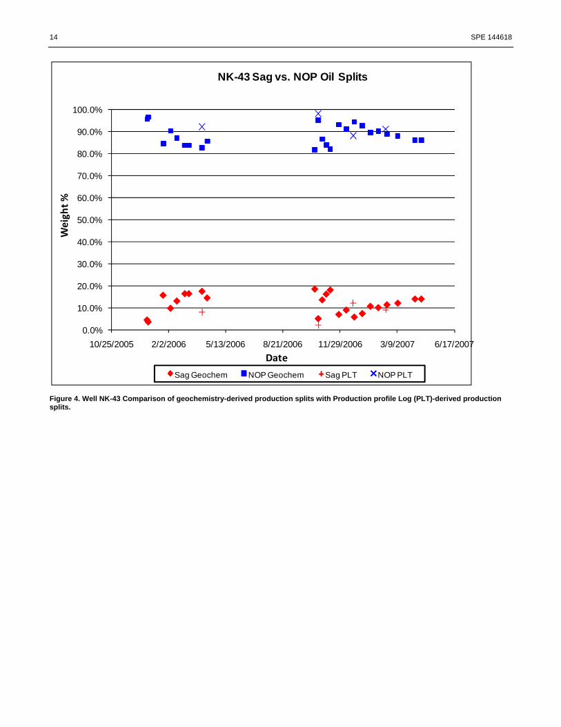
Issue 2: If one is seeking to allocate commingled gas being produced from multiple zones, and if liquid hydrocarbons are being co-produced with the gas from at least one of the zones, then the concentrations of the heavier hydrocarbon components in the gas may appear not to mix linearly. Non-linear mixing behavior of those gas components can be caused by partitioning of the heavier hydrocarbons either into the hydrocarbon liquids from the gas, or into the gas from the hydrocarbon liquids. The direction of partitioning (i.e., either into, or out of, the gas) is controlled by the compositions of the gases, the compositions of the hydrocarbon liquids, the ratio of the amount of gas to the amount of hydrocarbon liquids, the efficiency of contact of the gases with the hydrocarbon liquids, and the temperature and pressure. The magnitude of this non-ideal mixing of gas components will increase with increasing carbon number of the gas component. If water is being coproduced with the gas from at least one of the zones, then the concentration of CO2 in the gas may appear not to mix linearly due to partitioning of the CO2 either into or out of the water. CO2 in the water may then be lost by reaction with mineral phases. The geochemical parameters in a gas least affected by the gas/ liquid partitioning discussed above (and hence most useful for gas allocation studies) include: the concentrations of methane, ethane, and nitrogen, and the isotopic compositions of the methane, ethane, and nitrogen. Which of those parameters are most useful in any given study will depend on which parameters best distinguish the gas from the various zones being commingled. Although all four case studies presented below are oil allocation exercises, it is important to note that as long as the gas allocation issues discussed above are kept in mind, then exactly the same geochemical allocation approach which we apply to the four oil examples below can also be applied to gas allocation. Case Studies Over the last 11 years, we have geochemically allocated more than 1500 commingled oils from the North Slope of Alaska. Below we present four examples drawn from those studies, and all of the examples fall in the area shown in the map in Figure 3. Although the examples presented below only include 2-zone and 3-zone allocations, we routinely use the geochemical methodology to allocate commingled production from more than 3 zones, with 6 zones being the largest number that we have routinely allocated for a given well. Case Study #1: Well Niakuk-43 (NK-43), Greater Prudhoe Bay, North Slope, Alaska Well NK-43 was originally drilled and completed in February 2001. The Sag River (Sag) formation was perforated and tested first. A six-week-long production test period of the Sag was performed. During the test period, the Sag exhibited strong performance, with an average oil rate of 650 bbls per day. At this time, the Sag flowed without the assistance of gas lift. The Sag reservoir pressure at this time was 3,993 psi. On 5/4/2001, a cast iron bridge plug (CIBP) was set to isolate the Sag, and the Niakuk Oil Pool (NOP, Kuparuk formation) was then perforated. Kuparuk-only production took place from 5-6-2001 to 1-2-2006. As a feasibility study for applying geochemical production allocation to the NK-43 well, a blind test was performed in which the operator provided three “artificial mixtures” of NK-43 Sag oil and NK-43 Kuparuk oil. Using the geochemical approach described above, those artificial mixtures were allocated. After we reported the allocation results to the operator, the operator revealed the makeup of the 3 artificial mixtures. The difference between the geochemically derived allocation results and the composition of the artificial mixtures reported by the operator were 1.6%, 2.6%, and 1.0% (Table 1). The low errors in that blind test led the operator to then try a field study in which geochemical allocation was compared against production logs. The CIPB separating the Kuparuk and Sag was milled out 1-9-2006, and commingled production began 1/29/2006. During the course of a 6 month commingled testing period, four production profiles, 24 geochemical samples, 2 static bottom hole pressure surveys, and 43 well tests were gathered to assess performance of the Sag and Kuparuk intervals. The logging service company interpreted the oil, water and gas splits between the pools. OilTracers LLC interpreted oil splits using the new oil geochemical methodology, completely independent from the production logging analysis. Neither company was privy to the other’s analysis or results. A comparison of the commingled oil splits from both the production profiles and oil geochemical fingerprinting is presented in Figure 4.

SPE 144618 7

Upon completion of the six month commingled test period of the NOP and Sag, the well operator concluded that geochemical analysis had been demonstrated to provide an accurate and appropriate method of allocating oil between the NOP and the Sag. Therefore, the well operator prepared a report on the study results and proposed that from July 1, 2007 forward, geochemical fingerprinting be utilized for oil allocation purposes. The AOGCC concurred, and the NK-43 well has been periodically monitored by geochemical allocation since that date. A key advantage of geochemical allocation is illustrated by the fact that the 24 geochemical allocations that were performed on 24 different dates had a combined cost (for all 24) that was less than the cost of any one of the 4 production profiles that were run. Case Study #2: Well S-26, Prudhoe Bay Field, North Slope, Alaska

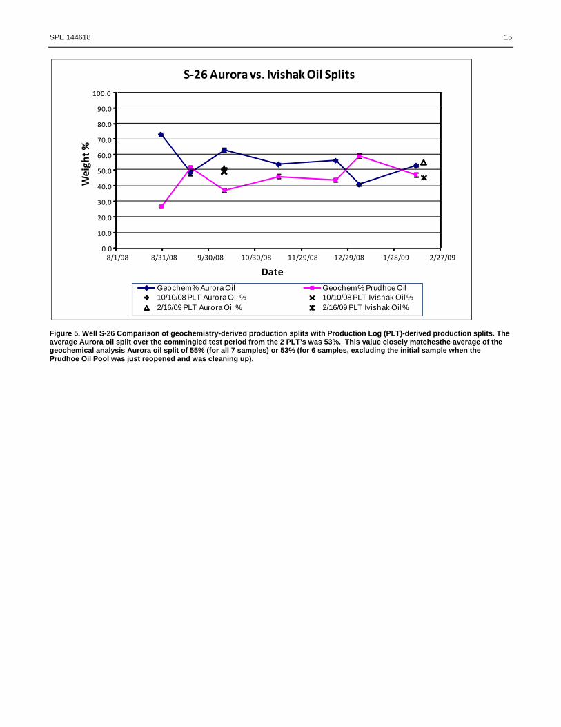
Well S-26 was originally drilled and completed as a Prudhoe Ivishak Zone 4 producer in 1990. Zone 4 was stimulated by both frac and acid treatments in 1991 and 1992 to maximize production. By late 2007, S-26 was producing 200 to 250 bopd at approximately 75% watercut and 6000 GOR from the Prudhoe Oil Pool. Well S-26 penetrates the Aurora Oil Pool and Prudhoe Oil Pool in areas where well rates from both pools are typically low. A stand-alone Aurora producer in this area could not be justified due to the expected low rates and associated problems with paraffin and hydrate deposition. Therefore, a Rig Workover (RWO) to commingle production from the two pools within the S-26 well-bore was planned to maximize oil production from the two oil pools. Prudhoe production was isolated on 12-15-2007. A Rig Workover to recomplete and enable Aurora production was completed in January 2008. Aurora perfs were added, and an initial Aurora-only SBHP was obtained on 4-3-2008. The Aurora reservoir pressure at this time was 3615 psi. The well was put on production on 4-4-2008. Total fluid rates were low, and the well was shut in on 4-7-2008. An Aurora-only frac job placed approximately 188,000 pounds of proppant in the formation on 5-12-08. The S-26 Aurora zone was put on production again on 5-16-08 with significantly increased production rates. As a feasibility study for applying geochemical production allocation to the S-26 well, a blind test was performed in which the operator provided three “artificial mixtures” of S-26 Ivishak oil and S-26 Aurora oil. Using the geochemical approach described above, those artificial mixtures were allocated. After we reported the allocation results to the operator, the operator revealed the makeup of the 3 artificial mixtures. The difference between the geochemically derived allocation results and the composition of the artificial mixtures reported by the operator were 6.2%, 3.9%, and 4.1% (Table 1). The low errors in that blind test led the operator to then try a field study in which geochemical allocation was compared against production logs. Plugs were drilled out to re-open the Prudhoe Oil Pool on 8-17-2008. Commingled production began on 8-20-2008; it has remained commingled since making approximately 600 bopd.The commingling of the Prudhoe and Aurora pools has had a positive impact on oil production from S-26. Over the course of a six month commingled test period (August 20, 2008 through February 20, 2008), the well operator fulfilled the Alaska Oil and Gas Conservation Commission’s requirements in obtaining Production Profiles, Static Bottom-Hole Pressure Surveys, Geochemical Samples and Well Tests. During the course of the commingled testing period, two production profile logs, 7 geochemical samples, and 19 well tests were gathered to assess performance of the Prudhoe and Aurora zones. The logging service company interpreted the oil, water and gas splits between the pools. OilTracers LLC interpreted oil splits using the new oil geochemical methodology, completely independent from the logging analysis. Neither company was privy to the other’s analysis or results. A comparison of the commingled oil splits from both the production profiles and oil geochemical fingerprinting is presented in Figure 5. Oil production splits obtained from the commingled geochemical samples are in close agreement with the Production profile logging results. The geochemical sample obtained on 10-10-2008 and the Production profile (PLT) started on 10-10-2008 were over 10 hours apart. Fluctuations in gas lift rates and well head pressures can have an impact on oil production splits from the 2 zones, explaining the slight variation in the more frequent geochemical analysis. The average Aurora oil split over the commingled test period from the 2 PLT’s was 53%. This value is a very close match to the average of the geochemical analysis Aurora oil split of 55% (average for all 7 samples) or 53% (average for 6 samples, excluding the initial sample when the Prudhoe Oil Pool was just reopened and was cleaning up).

Based on the good agreement between the geochemical and logging methods of measuring Aurora and Prudhoe oil splits, the well operator demonstrated that geochemical analysis provides an accurate and appropriate method of allocating oil between the two pools. A report of the findings was submitted to AOGCC by the well operator enabling geochemical fingerprinting to be utilized routinely for oil allocation of this well. Well S-26 has been periodically monitored by geochemical allocation since May 1, 2009.

8 SPE 144618

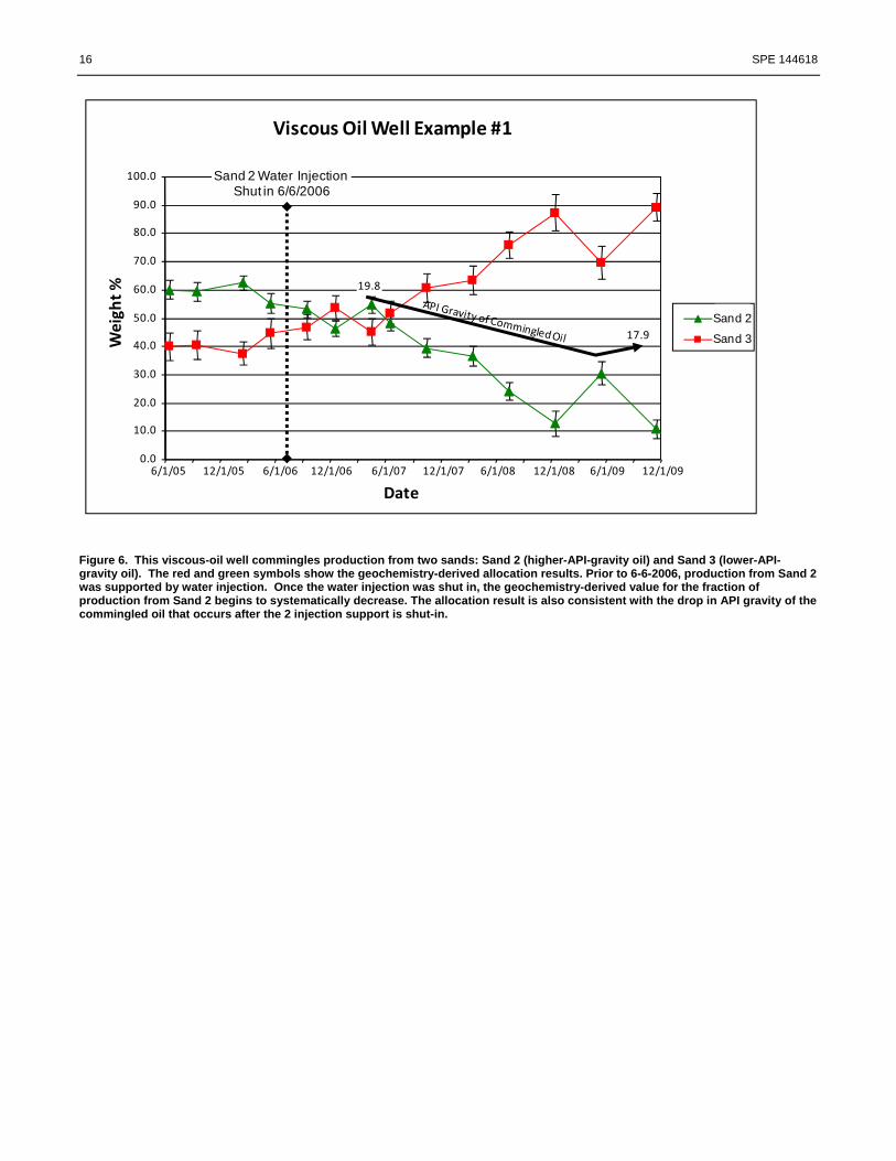
As in the previous case study, a key advantage of geochemical allocation is illustrated by the fact that the 7 geochemical allocations that were performed on 7 different dates had a combined cost (for all 7) that was far less than the cost of any one of the 2 PLT profiles that were run. Case Study #3, Viscous Oil Well #1, North Slope, Alaska Between 1999 and 2010, we have used the approach described in this paper to allocate the contribution of 2 or 3 sands to more than 800 commingled oil samples collected from more than 50 wells in a viscous oil accumulation on the North Slope of Alaska. This case study is drawn from one of those wells in that viscous oil accumulation. This example (Figure 6) demonstrates how geochemical allocation can be used to monitor the effect of shutting in water injection into a given zone. In this well, production streams from two sands are being commingled: Sand 2 (higher-API gravity-oil) and Sand 3 (lower-API-gravity oil). Prior to 6-6-2006, production from Sand 2 was supported by water injection. Once the water injection was shut in, the geochemistry-derived allocation results show that the production from Sand 2 begins to steadily decrease. The allocation result is also consistent with the drop in API gravity of the commingled oil that occurs after the water injection support into Sand 2 is shut-in. Case Study #4, Viscous Oil Well #2, North Slope, Alaska This case study is from a different well in the same field as Case Study #3. Figure 7 demonstrates how geochemical allocation can be used to monitor the effect of installing and removing an IsoSleeve over the perforations of a given zone. This well commingles production from three sands: Sand 1, Sand 2, and Sand 3. Between 7-28-2008 and 8-11-2008, an IsoSleeve was installed that attempted to shut off production from Sand 2. The IsoSleeve was removed on 9-20-2009. The geochemistry-derived allocation results show the fall in Sand 2 production after the IsoSleeve was installed, and show the return of Sand 2 production after the IsoSleeve was removed. On 10-10-2008, during the period the IsoSleeve was in place, a production log correctly determined that production from the well was dominated by Sand 3, but failed to detect the lesser production from Sand 1. In contrast, the geochemistry allocation technique was able to detect ~20% Sand 1 oil in the produced oil. The PLT was coiled-tubing conveyed, a method which can introduce significant back pressure. Back-pressure caused by the PLT tool is believed to have “turned off” production from Sand 1 during the logging run. The geochemistry method, since it does not involve inserting a tool into the well, does not create any back pressure, and hence is able to detect the true Sand 1 production. Discussion Advantages of Geochemical Allocation Compared to Production Logging There are many advantages to using oil geochemistry instead of production logging to allocate commingled production, including:

• Cost advantages relative to conventional e-line PLT: Geochemical techniques for allocating commingled production from multiple zones in a single well typically result in a >95% cost savings relative to conventional e-line production logging. The greater cost of the production logging approach is due not only to the costs of running the log, but also to the associated rig costs and the costs of lost production during logging. These costs are not applicable to the geochemical approach.

• Advantages relative to coiled tubing or tractor-conveyed e-line PLT: Cost savings from the geochemical approach are even more dramatic when compared to the costs of coiled-tubing-conveyed or tractor-conveyed PLT’s. Furthermore, the success rate of obtaining meaningful PLT data with a tractor conveyed e-line PLT is substantially less than 100%, a problem that does not affect geochemical allocation

• Detection of zone performance problems at any point during the life of a well: The low cost of the geochemical techniques for production allocation allows field engineers to monitor production frequently over long periods (e.g., weekly, monthly, quarterly). This ability to monitor continuously the relative performance of discrete pay zones allows early identification of zone performance problems. The much higher cost of production logging limits that technique to infrequent use; therefore, production logs typically provide only a "snap shot" of the production origin at the time the log was run, and not a continuous performance history.

• Applicability to vertical, deviated and horizontal wells: Geochemical techniques are applicable to highly deviated and horizontal wells in addition to vertical wells. In contrast, production logging interpretation is problematic in highly deviated wells. In some multi-lateral wells, where laterals off of laterals exist, there are often issues with lateral re-entry and thus production logging may not be capable of determining contribution from all zones.

SPE 144618 9

• Applicability to pumping wells: Geochemical techniques can be applied to all types of pumping wells (including those with tubing-deployed electrical submersible pumps, and progressive cavity pumps). In contrast, most pumping wells (except those with unusual completion styles, such as Y-block completions) cannot accommodate a production logging tool because the pumping apparatus prevents access of the logging tool to the underlying perforated interval.

• Ability to quantify uncertainty: Geochemical techniques provide multiple, independent solutions to the allocation problem, allowing one to quantify accurately the uncertainty of an allocation result. In contrast, the uncertainty associated with logging results is more difficult to quantify.

• Zonal Production vs. wellbore entry: Production allocation between zones is often used to assess oil remaining in the various layers for future development targets; therefore, it is critical to understand the source of the oil, and not just the section it entered the wellbore. Channels, near wellbore faults, and failed bores from initial drilling can create pathways by which oil from one zone can enter the wellbore at a depth associated with a different zone. Misallocation of oil can result in these situations if only wellbore entry is considered. Geochemical techniques are able to distinguish production from the various zones regardless of entry points.

• No risk of sticking a logging tool: Because the geochemical approach relies only on produced oil samples, obtained at surface, there is no risk of sticking a tool in the well.

The approach described here can also be used to assess the contribution of multiple fields to commingled pipeline production streams. The advantages of using geochemical allocation in such cases include:

• Ability to allocate in the absence of flow meter data: Geochemical techniques can allocate commingled production at points in the production stream where flow meter data are unavailable.

• Ability to identify problems with flow meter data: Where flow meter data are available, geochemical data provide complementary information for allocating production, because geochemical techniques measure the relative contributions of oil (instead of water + oil + gas) to a production stream. Since geochemical production allocation is not affected by entrained water, the geochemical techniques provide an independent check on allocation data from flow meters.

Issues Concerning End Member Oils Accurate geochemical allocation results require that the end member oils used in the allocation calculations truly represent the compositions of the oils from the zones that are being commingled. For example, consider a hypothetical case where oils from two zones are being commingled (Sand A and Sand B). To collect the “Sand B” end member, suppose the operator sets a bridge plug to isolate “Sand B”. Unknown to the operator, the bridge plug leaks, and the “Sand B” end member that the operator collects is actually contaminated with oil from “Sand A”. When that contaminated “Sand B” end member then is used to allocate a commingled “Sand A + Sand B” oil, the effect will be to erroneously raise the calculated allocation result for “Sand B” (Figure 8). Another common issue related to end member samples can be the lack of availability of end member oils collected from the same well from which the commingled oil was collected. To solve such a problem, the end member oil for a given sand may be collected from a well other than the commingled well, as long as the well from which the end member oil is collected penetrates the sand at a location that is in fluid communication with the commingled well. Sometimes an operator is able to acquire end member samples from all zones except one. Such a problem can be solved if a commingled sample is available for which independent evidence reveals the contribution of each zone to that commingled oil (for example, if a PLT was run close in time to when the commingled sample was collected). Under such circumstances, that commingled oil of known origin can itself be used as the “missing” end member oil for future geochemical allocation studies. More specifically, using that commingled sample along with the other end member oils, one can derive the composition of the one missing end member oil. It typically is not possible to solve a geochemical allocation problem if no end member oil samples are available. Sometimes the question is posed: “can the compositions of the end member oils be determined statistically from a large population of commingled oils, as long as all of the commingled oils are mixtures of the same (albeit unknown) end members?”. Typically, the answer is “no”. For example, consider the data in Figure 9. These data are not the results of actual analyses, but rather are hypothetical data used here to illustrate a concept. In both the left-hand panel and the right-hand panel, the data in the five blue columns are identical. Each blue column represents a commingled oil (Commingled oils B, C, H, D, and E), and each of these commingled oils is made up of different contributions from the same two unknown end members (Oil 1 and Oil 2). For each of those commingled oils, the GC peak heights of 10 GC peaks are measured, and hence each blue column has 10 rows. In the left hand panel (Solution 1), two hypothetical end member oils (Oil 1 and Oil 2) are shown in yellow that

10 SPE 144618

can be used to perfectly explain the blue data as perfect mixtures of Oil 1 and Oil 2. In that panel, for example, Oil H can be explained to be 85% Oil 1, 15% Oil 2. The right hand panel (Solution 2) derives completely different allocation results for the blue data, by simply changing the composition of the hypothetical end member “Oil 2”. In that panel, Oil H can be explained to be 44.44% Oil 1, 55.56% Oil 2. These same data are plotted in Figure 10, to further illustrate this concept. Without having true end member samples, there are an infinite number of possible allocation solutions to the blue data in Figure 9. The only way to derive the “true” allocation solutions for commingled oils B, C, H, D, and E is to have either (1) actual samples of the end member oils, or (2) a sample of one of the end member oils and a sample of a commingled oil for which the contribution of Oil 1 and Oil 2 is independently known. Summary As detailed here, we have made significant improvements to the previously published methods for geochemical allocation of commingled oil production and/or commingled gas production. This method has allowed allocation of commingled production from wells at less than 2-5% of the cost of production logging. Four case studies are shown here. In the first two case studies, commingling of the wells was subject to approval of a regulatory body. Before agreeing to the use of geochemical allocation, the regulating body required the well operator to perform multi-month trial studies in which the wells were monitored both by geochemical allocation and by production logging. The close agreement of the geochemically derived allocation results and the production-logging derived allocation results enabled regulatory approval of the on-going use of the geochemical allocation method for the allocation of oil between pools for these two wells. Two additional case studies presented here illustrate how geochemical allocation can be used to monitor the effects on production of (1) changes in water injection into nearby injectors, and (2) closing or opening perforations within a well. There are many advantages to using oil geochemistry instead of production logging to allocate commingled production, including: (1) significantly lower cost, (2) better ability to detect zone performance problems at any point during the life of a well, (3) applicability to vertical, deviated, horizontal, and multi lateral wells (4) applicability to pumping wells, (5) ability to quantify uncertainty, (6) applicability to wells with channels and (7) the absence of the risk of sticking a logging tool. References Hwang, R. J., D. K. Baskin and S. C. Teerman, “Allocation of commingled pipeline oils to field production,” Organic Geochemistry, v. 31,

2000, p.1463-1474. Kaufman, R. L., A. S. Ahmed and W. B. Hempkins, “A new technique for the analysis of commingled oils and its application to production

allocation calculations”. Paper IPA 87-23/21, 16th Annual Indonesian Petro. Assoc., 1987, p. 247-268. Kaufman, R. L., A.S. Ahmed and R.J. Elsinger, “Gas Chromatography as a development and production tool for fingerprinting oils from

individual reservoirs: applications in the Gulf of Mexico”. In: Proceedings of the 9th Annual Research Conference of the Society of Economic Paleontologists and Mineralogists. (D. Schumaker and B. F. Perkins, Ed.), New Orleans, 263-282, 1990

McCaffrey, M. A., H. A. Legarre and Johnson S. J., “Using biomarkers to improve heavy oil reservoir management: An example from the

Cymric field, Kern County, California,” AAPG Bulletin, v. 80, 1996, p. 904-919. Acknowledgements We thank BP Exploration Alaska Inc., ConocoPhillips Alaska Inc., and Weatherford Laboratories Inc. for permission to publish this work. In addition, the manuscript has benefited significantly from reviews by Alton A. Brown, Brian Seitz, James T. Rodgers, and David Jamieson.

SPE 144618 11

Table 1: Calculated Allocation Results Compared to Actual Compositions for Artificial Mixtures of Oils or Gases

Calculated Actual composition of Difference betw een GeochemicalNumber Type Allocation Artif ical Mixutre Calculated and Parameters Blind

Location of Zones Result Prepared by Laboratory Actual Composition Used Test?Well NK-43 2 Oil 13.4% / 86.6% 15.0% / 85.0% 1.6% 48 YesWell NK-43 2 Oil 47.5% / 52.5% 50.1% / 49.9% 2.6% 48 YesWell NK-43 2 Oil 78.9% / 21.1% 79.9% / 20.1% 1.0% 48 YesWell S-26 2 Oil 68.8% / 31.2% 75.0% / 25.0% 6.20% 132 YesWell S-26 2 Oil 46.1% / 53.9% 50.0% / 50.0% 3.90% 132 YesWell S-26 2 Oil 20.9% / 79.1% 25.0 % / 75.0% 4.10% 132 YesUndisclosed Alaska A 2 Oil 65.1% / 34.9% 66.5% / 33.5% 1.4% 209 YesUndisclosed Alaska A 2 Oil 87.1% / 12.9% 87.85% / 12.15% 0.75% 209 YesUndisclosed 0140 2 Oil 48.0% / 52.0% 50.1% / 49.9% 2.1% 40 YesUndisclosed 0140 2 Oil 51.5% / 48.5% 50.2% / 49.8% 1.3% 40 YesUndisclosed 0140 2 Oil 50.5 %/ 49.5% 49.9% / 50.1% 0.6% 40 YesUndisclosed 1053 2 Oil 90.4% / 9.6% 91.4% / 8.6% 1.0% 171 YesUndisclosed 1053 2 Oil 59.9% / 40.1% 59.6% / 40.4% 0.3% 171 YesUndisclosed 1053 2 Oil 87.2% / 12.8% 86.4% / 13.2% 0.8% 171 YesUndisclosed 1053 2 Oil 45.4% / 54.6% 44.3% / 55.7% 1.1% 171 YesUndisclosed 1053 2 Oil 60.2% / 39.8% 59.9% / 40.1% 0.3% 171 YesUndisclosed 1053 2 Oil 70.9% / 30.4% 70.2% / 29.8% 0.7% 171 YesAverage error of allocation of 2-zone artifical mixtures of oils in this table: 1.8%Undisclosed 1100 2 Gas 50.6% / 49.4% 50.0% / 50.0% 0.6% 8 NoUndisclosed 08834 3 Oil 60.2% / 39.8% / 0% 64.5% / 35.5% / 0% 4.3% / 4.3% / 0% 158 YesUndisclosed 08834 3 Oil 33.5% / 46.7% / 19.8% 39.1% / 40.9% / 20.0% 5.6% / 5.8% / 0.2% 158 YesUndisclosed 08692 3 Oil 49.2% / 28.9% / 21.9% 48.1% / 29.7% / 22.2% 1.1% / 0.8% / 0.3% 93 YesUndisclosed 08692 3 Oil 12.9% / 17.2% / 69.9% 10.8% / 19.7 % / 69.5% 2.1% / 2.5% / 0.4% 93 YesUndisclosed 0140 3 Oil 10.0% / 31.0% / 59.0% 15.0% / 29.9% / 55.1% 5.0% / 1.1% / 3.9% 40 YesUndisclosed 0140 3 Oil 54.0 %/ 15.0 %/ 31.0% 55.0% / 15.1% / 29.9% 1.0% / 0.1% / 1.1% 40 YesUndisclosed 48345 3 Oil 28.3% / 30.5% / 41.2% 31.0% / 29.9% / 39.1% 2.7% / 0.6% / 1.1% 138 YesUndisclosed 48345 3 Oil 20.1% / 22.2% / 57.7% 19.6% / 20.4% / 60.0 % 0.5% / 1.8% / 2.3% 138 YesAverage error of allocation of 3-zone artifical mixtures of oils in this table: 2.0%Undisclosed 0140 4 Oil 10.0% / 18.0% / 29.0% / 43.0% 10.0% / 19.9% / 29.8% / 40.3% 0.0% / 1.9% / 0.8% / 2.7% 40 YesUndisclosed 0140 4 Oil 18.0% / 25.0% / 36.0% / 19.0% 19.8% / 29.9% / 39.1% / 10.6% 1.8% / 4.9% / 3.1% / 8.4% 40 YesUndisclosed 0140 4 Oil 42.0% / 7.0% / 17.0% / 34.0% 40.1% / 10.2% / 19.8% / 29.9% 1.9% / 3.2 % / 2.8 %/ 4.1% 40 YesUndisclosed 48345 4 Oil 30.7% / 25.9% / 11.0% / 32.4% 30.0% / 30.0% / 10.0% / 30.0% 0.7% / 4.1% / 1.0% / 2.4% 137 YesUndisclosed 48345 4 Oil 30.0% / 43.1% / 7.7%/ 19.2% 26.3% / 43.7% / 12.7% / 17.2% 3.7% / 0.6%/ 5.0% / 2.0% 137 YesUndisclosed 48345 4 Oil 9.6% / 10.3% / 39.1% / 41.0% 10.0 % / 10.0% / 40.0% / 40.0% 0.4% / 0.3% / 0.9% / 1.0% 137 YesUndisclosed 48345 4 Oil 21.0% / 26.9% / 22.7% / 29.4% 20.3% / 29.5% / 20.0% / 30.2% 0.7% / 2.6% / 2.7% / 0.8% 137 YesAverage error of allocation of 4-zone artifical mixtures of oils in this table: 2.3%

12 SPE 144618

V

I

II III and IVLines Superimposed

frac

(2) 

frac (1) 1.5

0.75

1.0

1.0

Figure 1. The lines representing the 5 equations intersect at a unique point (a point corresponding to the allocation solution). This figure demonstrates a difference between projects that do and do not use isotope data: Where only concentration data are used, every equation is a line with a negative slope with positive intercepts on both axes. In the general case, every equation forms a hyperplane in n-dimensions (where n is the number of end-members) with positive intercepts on each dimension. In contrast, the equations that govern mixing of isotopic values are lines that pass through the origin. In the general case, equations that govern mixing of isotopic values describe hyperplanes in n-dimensions (where n is the number of end-members) that pass through the origin.

Figure 2. The lines representing the 5 equations do not intersect at a unique point because we introduced “error” into the isotope data for the commingled gas. Linear algebra (i.e., a least squares regression) can then be used to derive the best “compromise” solution in a manner just as was described previously for the allocation of commingled oils.

SPE 144618 13

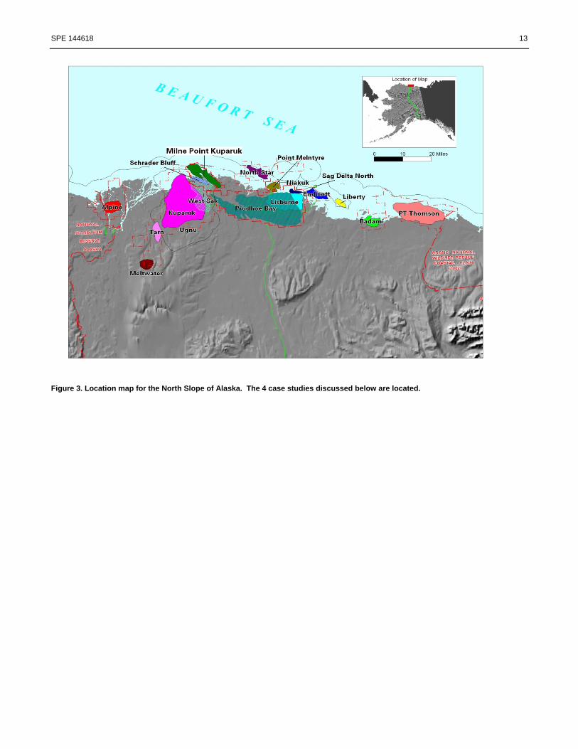
Figure 3. Location map for the North Slope of Alaska. The 4 case studies discussed below are located.

14 SPE 144618

0.0%

10.0%

20.0%

30.0%

40.0%

50.0%

60.0%

70.0%

80.0%

90.0%

100.0%

10/25/2005 2/2/2006 5/13/2006 8/21/2006 11/29/2006 3/9/2007 6/17/2007

NK-43 Sag vs. NOP Oil Splits

Sag Geochem NOP Geochem Sag PLT NOP PLT

Weigh

t %

Date

Sag Geochem NOP Geochem Sag PLT NOP PLT

Figure 4. Well NK-43 Comparison of geochemistry-derived production splits with Production profile Log (PLT)-derived production splits.

SPE 144618 15

ight

%

0.0

10.0

20.0

30.0

40.0

50.0

60.0

70.0

80.0

90.0

100.0

8/1/08 8/31/08 9/30/08 10/30/08 11/29/08 12/29/08 1/28/09 2/27/09

Geochem% Aurora Oil Geochem % Prudhoe Oil10/10/08 PLT Aurora Oil % 10/10/08 PLT Ivishak Oil %2/16/09 PLT Aurora Oil % 2/16/09 PLT Ivishak Oil %

Weigh

t %

Date

S‐26 Aurora vs. Ivishak Oil Splits

Figure 5. Well S-26 Comparison of geochemistry-derived production splits with Production Log (PLT)-derived production splits. The average Aurora oil split over the commingled test period from the 2 PLT’s was 53%. This value closely matchesthe average of the geochemical analysis Aurora oil split of 55% (for all 7 samples) or 53% (for 6 samples, excluding the initial sample when the Prudhoe Oil Pool was just reopened and was cleaning up).

16 SPE 144618

1E‐121 Production Allocation Results

0.0

10.0

20.0

30.0

40.0

50.0

60.0

70.0

80.0

90.0

100.0

Wt %

Sand 2 Water Injection Shut in 6/6/2006

19.8

Sand B

Sand D17.9

Viscous Oil Well Example #1

Sand 2

Sand 3

Date

Weigh

t %

6/1/05 12/1/05 6/1/06 12/1/06 6/1/07 12/1/07 6/1/08 12/1/08 6/1/09 12/1/09

Figure 6. This viscous-oil well commingles production from two sands: Sand 2 (higher-API-gravity oil) and Sand 3 (lower-API-gravity oil). The red and green symbols show the geochemistry-derived allocation results. Prior to 6-6-2006, production from Sand 2 was supported by water injection. Once the water injection was shut in, the geochemistry-derived value for the fraction of production from Sand 2 begins to systematically decrease. The allocation result is also consistent with the drop in API gravity of the commingled oil that occurs after the 2 injection support is shut-in.

SPE 144618 17

1J-166 Production Allocation Results

0.0

10.0

20.0

30.0

40.0

50.0

60.0

70.0

80.0

90.0

100.0

Wt %

Sand ASand B

Sand D

Viscous Oil Well Example #2

Sand 2

Sand 3

Date

Weigh

t %

Sand 1

PLT10/10/2008

Sand 2 IsoSleeveRemoved 9/20/2009

Sand 2 IsoSleeveInstalled 7/25/-8/18/2008

4/3/06 8/3/06 12/3/06 4/3/07 8/3/07 12/3/07 4/3/08 8/3/0812/3/08 4/3/09 8/3/09

Figure 7. This viscous-oil well commingles production from three sands: Sand 1, Sand 2, and Sand 3. Between 7-28-2008 and 8-11-2008, an IsoSleeve was installed that shut off production from Sand 2. The IsoSleeve was removed on 9-20-2009. The geochemistry-derived allocation results (small red, green, and blue symbols) show the fall in Sand 2 production after the IsoSleeve was installed, and show the return of Sand 2 production after the IsoSleeve was removed. During the period the IsoSleeve was in place, a PLT that was run (10-10-2008; large red, green, and blue symbols)) failed to detect production from Sand 1, although the geochemistry was able to detect ~20% Sand 1 production. Back-pressure caused by the PLT tool is believed to be the cause of the PLT being unable to detect the Sand 1 production. The geochemistry method, since it does not involve inserting a tool into the well, does not create any back pressure, and hence is able to detect the Sand 1 production.

18 SPE 144618

Figure 8. Inadvertent “contamination” of a “Sand B” end member with oil from “Sand A” will raise the apparent contribution of “Sand B” to any commingled “Sand A+ Sand B” oils that are allocated using the contaminated “Sand B” end member. This concept is illustrated by the two diagrams shown above. In the top diagram, both end members oils are pure oil from their respective zones. The commingled oil in that diagram has a composition exactly half way between the compositions of the two end members, and is correctly allocated as a 50%/50% mix of oil from Sand A and Sand B. In the bottom diagram, the Sand B end member is “contaminated” with 25% Sand A oil. The effect of this contamination on the allocation result is to erroneously increase the calculated “Sand B” contribution to 67%.

Oil 1 Mix B Mix C Mix H Mix D Mix E Oil 2 Oil 1 Mix B Mix C Mix H Mix D Mix E Oil 2%Oil 2 0 5 10 15 20 25 100 %Oil 2 0 18.52 37.04 55.56 74.07 92.59 100

Height Peak 1 114.00 121.75 129.50 137.25 145.00 152.75 269.00 Height Peak 1 114.00 121.75 129.50 137.25 145.00 152.75 155.85Height Peak 2 158.00 164.30 170.60 176.90 183.20 189.50 284.00 Height Peak 2 158.00 164.30 170.60 176.90 183.20 189.50 192.02Height Peak 3 126.00 130.50 135.00 139.50 144.00 148.50 216.00 Height Peak 3 126.00 130.50 135.00 139.50 144.00 148.50 150.30Height Peak 4 236.00 232.40 228.80 225.20 221.60 218.00 164.00 Height Peak 4 236.00 232.40 228.80 225.20 221.60 218.00 216.56Height Peak 5 277.00 275.40 273.80 272.20 270.60 269.00 245.00 Height Peak 5 277.00 275.40 273.80 272.20 270.60 269.00 268.36Height Peak 6 130.00 132.25 134.50 136.75 139.00 141.25 175.00 Height Peak 6 130.00 132.25 134.50 136.75 139.00 141.25 142.15Height Peak 7 283.00 282.35 281.70 281.05 280.40 279.75 270.00 Height Peak 7 283.00 282.35 281.70 281.05 280.40 279.75 279.55Height Peak 8 172.00 169.05 166.10 163.15 160.20 157.25 113.00 Height Peak 8 172.00 169.05 166.10 163.15 160.20 157.25 156.07Height Peak 9 143.00 147.55 152.10 156.65 161.20 165.75 234.00 Height Peak 9 143.00 147.55 152.10 156.65 161.20 165.75 167.57Height Peak 10 149.00 150.60 152.20 153.80 155.40 157.00 181.00 Height Peak 10 149.00 150.60 152.20 153.80 155.40 157.00 157.64

Solution 1 Solution 2

Figure 9. These data are not the results of actual analyses, but rather are hypothetical data used here to illustrate a concept. In both the left-hand panel and the right hand panel, the data in the five blue columns are identical. Each blue column represents a commingled oil (Commingled oils B, C, H, D, and E), and each of these commingled oils is made up of different contributions from the same two unknown end members (Oil 1 and Oil 2). For each of those commingled oils, the GC peak heights of 10 GC peaks are measured, and hence each blue column has 10 rows. In the left hand panel (Solution 1), two hypothetical end member oils (Oil 1 and Oil 2) are shown in the yellow columns, and those hypothetical end members can be used to perfectly explain the blue data as perfect mixtures of Oil 1 and Oil 2 (with the values shown in red). In that panel, for example, Oil H can be explained to be 85% Oil 1, 15% Oil 2. The right-hand panel (Solution 2) derives completely different allocation results for the blue data, by simply changing the composition of the hypothetical end member “Oil 2”. In that panel, Oil H can be explained to be 44.44% Oil 1, 55.56% Oil 2. These data are plotted in Figure 10.

SPE 144618 19

0.00

50.00

100.00

150.00

200.00

250.00

300.00

0 10 20 30 40 50 60 70 80 90 100

Peak 1

Peak 2

Peak 3

Peak 4

Peak 5

Peak 6

Peak 7

Peak 8

Peak 9

Peak 10

GC Peak Height

% Oil 2 in Mixture

Mix B

Mix C

Mix H

Mix D

Mix E

Solution 1

0.00

50.00

100.00

150.00

200.00

250.00

300.00

0 10 20 30 40 50 60 70 80 90 100

Peak 1

Peak 2

Peak 3

Peak 4

Peak 5

Peak 6

Peak 7

Peak 8

Peak 9

Peak 10

GC Peak Height

% Oil 2 in Mixture

Mix B

Mix C

Mix H

Mix D

Mix E

Solution 2

Figure 10. The upper panel in this figure plots “Solution 1” from Figure 9. The lower panel in this figure plots “Solution 2” from Figure 9. These figures illustrate that without having true end member samples, there are an infinite number of possible allocation solutions to the blue data in Figure 9.