spatiotemporal pattern formation in neural ﬁelds with...

Spatiotemporal pattern formation in neuralfields with linear adaptation

G. Bard Ermentrout, Stefanos E. Folias, and Zachary P. Kilpatrick

Abstract We study spatiotemporal patterns of activity that emerge inneural fields inthe presence of linear adaptation. Using an amplitude equation approach, we showthat bifurcations from the homogeneous rest state can lead to a wide variety of sta-tionary and propagating patterns, especially in the case oflateral-inhibitory synap-tic weights. Typical solutions are stationary bumps, traveling bumps, and stationarypatterns. However, we do witness more exotic time-periodicpatterns as well. Usinglinear stability analysis that perturbs about stationary and traveling bump solutions,we then study conditions for activity to lock to the positionof an external input.This analysis is performed in both periodic and infinite one-dimensional spatial do-mains. Both Hopf and saddle-node bifurcations can signify the boundary beyondwhich stationary or traveling bumps fail to lock to externalinputs. Just beyond Hopfbifurcations, bumps begin to oscillate, becomingbreatheror sloshersolutions.

1 Introduction

Neural fields that include local negative feedback have proven very useful inqualitatively describing the propagation of experimentally observed neural activ-ity [26, 39]. Disinhibitedin vitro cortical slices can support traveling pulses andspiral waves [27, 53], suggesting that some process other than inhibition must cur-

G. Bard ErmentroutUniversity of Pittsburgh, Department of Mathematics, Pittsburgh PAe-mail: [email protected]

Stefanos E. FoliasUniversity of Alaska Anchorage, Department of Mathematical Sciences, Anchorage AKe-mail: [email protected]

Zachary P. KilpatrickUniversity of Houston, Department of Mathematics, HoustonTXe-mail: [email protected]

1

2 G. Bard Ermentrout, Stefanos E. Folias, and Zachary P. Kilpatrick

tail large-scale neural excitations. A common candidate for this negative feedbackis spike frequency adaptation, a cellular process that brings neurons back to theirresting voltage after periods of high activity [48, 2]. Often, adaptation is modeledas an additional subtractive variable in the activity equation of a spatially extendedneural field [38, 26, 39]. Pinto, in his PhD dissertation withErmentrout, exploredhow linear adaptation leads to the formation of traveling pulses [38]. Both singularperturbation theory and the Heaviside formalism of Amari [1] were used to an-alyze an excitatory network on the infinite spatial domain [38, 39]. At the sametime, Hansel and Sompolinsky showed adaptation leads to traveling pulses (travel-ing bumps) in a neural field on the ring domain [26]. In the absence of adaptation,excitatory neural fields generate stable traveling fronts [21, 25]. For weak adapta-tion, the model still supports fronts which undergo a symmetry breaking bifurca-tion, leading to bidirectional front propagation at a critical value of the adaptationrate [6]. In fact, adaptive neural fields generate a rich variety of spatiotemporal dy-namics like stimulus-induced breathers [7], spiral waves [27], multipulse solutions[52], and self-sustained oscillations [46]. Coombes and Owen have implemented arelated model, employing nonlinear adaptation, that is shown to generate breathers,traveling bumps, and more exotic solutions [11]. However, it has been shown thatgreat care must taken when performing stability analysis ofsuch a model [29]. Thus,we restrict the contents of this chapter to analyzing modelswith linear adaptation.

We review a variety of results concerning bifurcations thatarise in spatially ex-tended neural fields when an auxiliary variable representing linear adaptation isincluded [13, 23, 25, 31]. In particular, we study the dynamics of the system ofnon-local integro-differential equations [26, 39, 35, 10]

τ∂u(x, t)

∂ t=−u(x, t)−βv(x, t)+

∫

Dw(x− y)F(u(y, t))dy+ I(x, t), (1a)

1α

∂v(x, t)∂ t

= u(x, t)− v(x, t). (1b)

The variableu(x, t) represents the total synaptic input arriving at locationx ∈ Din the network at timet. We can fix time units by settingτ = 1, without loss ofgenerality. The convolution term represents the effects ofrecurrent synaptic interac-tions, andw(x− y) = w(y− x) is a reflection-symmetric synaptic weight encodingthe strength of connections between locationy andx. The nonlinearityF is a trans-fer function that converts the synaptic inputs to an output firing rate. Local negativefeedbackv(x, t) represents the effects of spike frequency adaptation [26, 48, 39, 2],occurring at rateα with strengthβ . Finally, I(x, t) represents external spatiotempo-ral inputs. In section 2, we begin by analyzing bifurcationsfrom the rest state on one-and two-dimensional periodic domains, in the absence of inputs (I(x, t) ≡ 0) withthe use of amplitude equations. We show that a lateral-inhibitory synaptic weightorganizes activity of the network into a wide variety of stationary and propagatingspatiotemporal patterns. In section 3, we study the processing of external inputs byin ring domain (D = (−π ,π)). Since adaptation can lead to spontaneous propaga-tion of activity, inputs must move at a speed that is close to the natural wavespeed

Spatiotemporal pattern formation in neural fields with linear adaptation 3

of the network to be well tracked by its activity. Finally, insection 4, we studybifurcations of stationary and traveling bumps in a networkon the infinite spatialdomain (D = (−∞,∞)). Both natural and stimulus-induced bump solutions are an-alyzed. Depending on whether the synaptic weight function is purely excitatory orlateral-inhibitory, either spatial mode of a stimulus-locked bump can destabilize ina Hopf bifurcation, leading to abreatheror aslosher. Conditions for the locking oftraveling bumps to moving inputs are discussed as well.

2 Bifurcations from the homogeneous state.

The simplest type of analysis that can be done with continuumneural field modelsis to study bifurcations from the homogeneous state. As in [13], we focus on theone-dimensional ring model, and then make some comments about the dynamicsof systems in two space dimensions with periodic boundary conditions. Here, ourdomain is either the ring (D = (−π ,π)) or the square (D = (−π ,π)× (−π ,π))with periodic boundary conditions. With some abuse of notation,x is either a scalaror a two-dimensional vector. The functionw(x) is periodic in its coordinates andfurthermore, we assume that it is symmetric in one-dimension and isotropic in two-dimensions. Translation invariance and periodicity assures us that

∫

D w(x− y)dy=W0. A constant steady state has the form

u(x, t) = u, where (1+β )u=W0F(u).

SinceF is monotonically increasing withF(−∞) = 0 andF(+∞) = 1, we areguaranteed at least one root. To simplify the analysis further, we assume thatF(u) = k( f (u)− f (0))/ f ′(0) with f (u) = 1/(1+exp(−r(u−uth))) as in [13]. Notethat F(0) = 0 andF ′(0) = k which serves as our bifurcation parameter. With thisassumption, ¯u= v= 0 is the homogeneous rest state.

To study the stability, we linearize, lettingu(x, t) = u+q(x, t) andv(x, t) = u+p(x,y) so that to linear order inq(x, t), p(x, t) we have

∂q∂ t

= −q(x, t)+ k∫

Ωw(x− y)q(y, t) dy−β p(x, t) (1)

∂ p∂ t

= α(−p(x, t)+q(x, t)).

Becausew(x) is translational invariant and the domain is periodic, solutions to thelinearized equations have the form exp(λ t)exp(in · x) where in one-dimensionn isan integer and in two-dimensions, it is a pair of integers,(n1,n2). Let m= |n| be themagnitude of this vector (scalar) and let

W(m) :=∫

Ωw(y)e−in·y dy.


(The isotropy ofw guarantees that the integral depends only on the magnitude of n.)We then see thatλ must satisfy

λ(

χ1

χ2

)

=

(

−1+ kWm −βα −α

)(

χ1

χ2

)

, (2)

where(χ1,χ2)T is a constant eigenvector.

There are several cases with which to contend, and we now describe them. Theeasiest parameter to vary in this system is the sensitivity,k (This is the slope ofF atthe equilibrium point). The trace of this matrix isT (m) :=−(1+α)+kW(m) andthe determinant isD(m) :=α[1+β −kW(m)]. Note thatW(0) =W0 andW(m)→ 0asm→∞. The uniform state is linearly stable if and only ifT (m)< 0 andD(m)>0for all m. If W(m) < 0, then both stability conditions hold, so, consider the setskT

m = (1+α)/W(m) andkDm = (1+β )/W(m) which represent critical values ofk

where the trace and determinant vanish respectively. We areinterested in the min-imum of these sets over all values ofm whereW(m) > 0. Let n denote the criticalwavenumber at whichW(m) is maximal. It is clear that ifα > β then the deter-minant vanishes at a lower value ofk than the trace does andvice versa.Thatis, there is a critical ratioR= β/α such that ifR> 1, then the trace is critical(and there is a Hopf bifurcation) while ifR< 1, the determinant is critical (andthere is a stationary bifurcation). The ratioR is the product of the strength andthe time constant of the adaptation. If the adaptation is weak and fast, there is asteady state bifurcation, while if it is large and slow, there is a Hopf bifurcation.[13] studied the special case whereR is close to 1. AtR= 1, there is a doublezero eigenvalue at the critical wavenumberm and thus a Takens-Bogdanov bifur-cation. For the rest of this section, letm∗ denote the value of|n| at whichW(m)is maximal. We also assume thatW(m∗) > 0. For one dimension,n= ±m∗ and in

two spatial dimensions, at criticality,n= (n1,n2) wherem∗ =√

n21+n2

2. For con-

creteness and illustration of the results, we usef (u) = 1/(1+ exp(−r(u− uth)))with two free parameters that set the shape off and thusF. We remark that (i)if uth = 0, thenF ′′(0) = 0 and (ii) for a range ofuth surrounding 0,F ′′′(0) < 0.We also usew(x) = Aap/2exp(−ax2)−Bbp/2exp(−bx2) (where p is the dimen-sion of the domain and note thatW(m) = π(Aexp(−m2/a)−Bexp(−m2/b)). WithA= 5,a= .125,B= 4,b= .005, this kernel has a fairly narrow Mexican hat profile.

2.1 One spatial dimension.

2.1.1 Zero eigenvalue.

In the case ofR< 1, the bifurcation is at a zero eigenvalue and we expect a spa-tial pattern that has the formu(x, t) = zexp(im∗x) + c.c (here c.c means complexconjugates) and

zt = z(a(k− kc)−b|z|2)


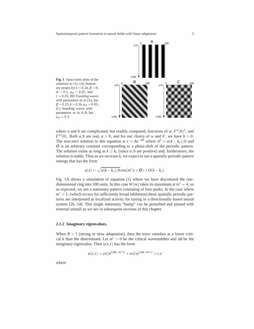
Fig. 1 Space-time plots of thesolutions to (1). (A) Station-ary stripes fork= 0.24,β = 0,α = 0.1, uth = 0.05, andr = 0.25; (B) Traveling waveswith parameters as in (A), butβ = 0.25,k= 0.26,uth= 0.05;(C) Standing waves withparameters as inA,B, bututh = 0.3.

t=01000

t=01000

A

CB

t=01000

t=50

t=50 t=50

wherea andb are complicated, but readily computed, functions ofw, F ′′(0)2, andF ′′′(0). Both a,b are real,a > 0, and for our choice ofw andF , we haveb > 0.The non-zero solution to this equation isz= Ae−iΘ whereA2 = a(k− kc)/b andΘ is an arbitrary constant corresponding to a phase-shift of the periodic pattern.The solution exists as long ask ≥ kc (sincea,b are positive) and, furthermore, thesolution is stable. Thus as we increasek, we expect to see a spatially periodic patternemerge that has the form

u(x) =√

a(k− kc)/bcos(m∗x+Θ)+O(k− kc).

Fig. 1A shows a simulation of equation (1) where we have discretized the one-dimensional ring into 100 units. In this caseW(m) takes its maximum atm∗ = 4, soas expected, we see a stationary pattern consisting of four peaks. In the case wherem∗ = 1, (which occurs for sufficiently broad inhibition) these spatially periodic pat-terns are interpreted as localized activity for tuning in a directionally based neuralsystem [26, 54]. This single stationary “bump” can be perturbed and pinned withexternal stimuli as we see in subsequent sections of this chapter.

2.1.2 Imaginary eigenvalues.

WhenR> 1 (strong or slow adaptation), then the trace vanishes at a lower criti-cal k than the determinant. Letm∗ > 0 be the critical wavenumber andiω be theimaginary eigenvalue. Thenu(x, t) has the form

u(x, t) = z(t)ei(ωt−m∗x)+w(t)ei(ωt+m∗x)+ c.c

where


z′ = z[(a1+ ia2)(k− kc)− (b1+ ib2)|z|2− (c1+ ic2)|w|2] (3)

w′ = w[(a1+ ia2)(k− kc)− (b1+ ib2)|w|2− (c1+ ic2)|z|2].

These coefficients can be computed for (1) (and, indeed, for avariant of the equa-tions [13] computes them explicitly) and they depend only onF ′′(0)2 , F ′′′(0),W(2m), W(m), α, andβ . In particular, with our choice off (u) and for uth notlarge, b1,c1 > 0. There are three distinct types of nontrivial solutions:(z,w) =(Z,0),(0,Z),(Y,Y), where:

Z = AeiΩt , A2 = (a1/b1)(k− kc),Ω = (a2−a1b2/b1)(k− kc), Y = BeiΞ t ,B2 = (a1/(b1+ c1))(k− kc), Ξ = (a2−a1(b2+ c2)/(b1+ c1))(k− kc).

Solutions of the form(Z,0),(0,Z) correspond to traveling wavetrains with oppositevelocities and those of the form(Y,Y) correspond to standing time-periodic waves.To see this, we note that the solutions have the form

u(x, t) = ℜzei(ωt+m∗x)+wei(ωt−m∗x),

so that for the solution,(Z,0), we get

u(x, t) = Acos((ω +Ω)t +m∗x),

while for the(Y,Y) case

u(x, t) = Bcos((ω +Ξ)t)cos(m∗x).

The traveling (standing) waves are stable if and only ifc1 > b1 (resp.c1 < b1) and,importantly, ifF ′′(0) is zero or close to zero (that is,uth ≈ 0), thenc1 > b1 no matterwhat you choose for the other parameters. Thus, foruth small, we expect to see onlystable traveling waves. Fig. 1B,C shows simulations of (1) for two different choicesof uth; near zero, the result is traveling waves, while foruth = 0.3, standing wavesemerge. Choosing the interaction kernel,w(x), so thatm∗ = 1, leads to a singletraveling pulse or bump of activity which, itself, can be entrained and perturbed byexternal stimuli (see the next sections).

2.2 Two-dimensions.

While most of the focus in this chapter is on one space dimension, the theory ofpattern formation is much richer in two-dimensions and equation (1) provides anexcellent example of the variety of patterns. The isotropy of the weight matrix im-plies that the eigensolutions to the linear convolution equation (1) have the formexp(in ·x). In two dimensions,n is a two-vector of integers. We then obtain exactlythe same formula for the determinant and the trace as in one-dimension, however,


Fig. 2 Three different casesof critical wavenumbers inthe square lattice. The criticalwavenumbers are (from outto in), (±1,0), (0,±1),(±2,1), (±2,−1),(±1,2), (±1,−2)and(±3,4), (±3,−4),(±4,3), (±4,−3),(±5,0), (0,±5).

=

*m*= 1

m*

= 5

5

m

m= |n| in this case so that there are at least two distinct eigenvectors and their com-plex conjugates and there are often many more. Fig. 2 illustrates three cases wherem∗ = 1,

√5,5 corresponding to four, eight, and twelve different pairs(n1,n2). We

treat and numerically illustrate several possibilities bydiscretizing (1) on a 50×50array. Our choice ofw(x) gives a maximum atm∗ = 2 which is the simplest case.

2.2.1 Zero eigenvalue.

The simplest possible case in two dimensions has only four distinct wave vectors (in-ner circle in Fig. 2). For example, ifm∗ = 2, thenn∈(2,0),(0,2),(−2,0),(0,−2).(Note that in those cases where there are only four vectors, the critical waves musthave either of the two forms,(k,0),(0,k),(−k,0),(0,−k) or (k,k),(k,−k),(−k,−k),(−k,k).)If we write x = (x1,x2), then, u(x, t) has the formu(x1,x2, t) = z1exp(i2x1) +z2exp(i2x2)+ c.c and

z′1 = z1(a(k− kc)−b|z1|2− c|z2|2), (4)

z′2 = z2(a(k− kc)−b|z2|2− c|z1|2),

where as in the one-dimensional case,b,cdepend onF ′′(0)2,F ′′′(0).All coefficientsare real and can be computed. They are all positive for our choices ofF(u). We letzj = A jeiΘ j and we then find that

A′1 = A1(a(k− kc)−bA2

1− cA22),

A′2 = A2(a(k− kc)−bA2

2− cA21).

It is an elementary calculation to show that there are three types of solutions,(z1,z2) = (r1,0),(0, r1),(r2, r2) wherer2

1 = a(k− kc)/b andr22 = a(k− kc)/(b+

c). For this example, the first two solutions correspond to vertical and horizontalstripes respectively and the third solution represents a spotted or checkerboard pat-tern. Stripes (spots) are stable if and only ifb < c (resp.b > c) [16]. As in thetraveling/standing wave case above, ifF ′′(0) is zero (uth = 0), then,c> b and thereare only stable stripes [16]. The resulting stationary patterns look identical to those


in Fig. 3A,B without the implied motion. (To get stationary patterns, choose, e.g.,β = 0, r = 3, anduth = 0 for stripes oruth = 0.3 for spots .)

This case (of two real amplitude equations) is the simplest case. The criti-cal wave vector can be more complicated, for example, ifm∗ =

√5, then,n ∈

(1,2),(1,−2),(2,1),(2,−1),(−1,−2),(−1,2),(−2,−1),(−2,1) for which thereare eight eigenvectors and the solution has the form

u(x, t) =4

∑j=1

zj(t)ein j ·x+ c.c,

wheren j = (1,2), . . . andzj satisfy the four independent amplitude equations

z′1 = z1(a(k− kc)−b|z1|2− c|z2|2−d|z3|2−e|z4|2),z′2 = z2(a(k− kc)−b|z2|2− c|z1|2−d|z4|2−e|z3|2),z′3 = z3(a(k− kc)−b|z3|2− c|z4|2−d|z1|2−e|z2|2),z′4 = z4(a(k− kc)−b|z4|2− c|z3|2−d|z2|2−e|z2|2).

As in equations (4), sincea, . . . ,eare all real coefficients, this model can be reducedto the analysis of a four dimensional real system. [15] derive and analyze this case(among many others). In the context of neural fields, Tass [49] and Ermentrout [17]provide stability conditions for the equilibria, all of which consist ofzj taking onvalues of someA 6= 0 or 0. For example, the pure patternsz1 = A, z2,z3,z4 = 0 arestable if and only ifa< b,c,d, there are also pairwise mixed solutions (checker-boards) of the formz1 = z2 = A′, z3 = z4 = 0, etc, and fully nonzero solutions,z1 = z2 = z3 = z4 = A′′ which are stable ifa > d+ c− b,d+ b− c,b+ c− d.We remark that the triplet solutionszj = zk = zl = A′′′ are never stable and that ifF ′′(0) = 0, then only stripes (onezj , nonzero).

In two spatial dimensions,m∗ = 1 can correspond to a single bump of activitywhich has been used to model hippocampal place cells [28]. For narrower inhibition,the more complex patterns describe the onset of geometric visual hallucinations[18, 49, 50, 5]. Simple geometric hallucinations take the form of spirals, pinwheels,bullseyes, mosaics, and honeycombs [33]. When transformedfrom the retinocentriccoordinates of the eyeball to the coordinates of the visual cortex, these patterns takethe form of simple geometric planforms such as rolls, hexagons, squares, etc. [45]Thus, spontaneous bifurcations to patterned activity forma natural model for thesimple visual patterns seen when the visual system is perturbed by hallucinogens,flicker [43] or other excitation. (See [3] for a comprehensive review.)

2.2.2 Imaginary eigenvalues.

The case of imaginary eigenvalues on a square lattice is quite complicated and onlypartially analyzed. [50] has studied this case extensivelywhen there are no eventerms in the nonlinear equations (corresponding tout = 0 in our model. [47] provide


a comprehensive and extremely readable analysis of of case where there are fourcritical wavenumbers.

Let us first consider the four dimensional case and take as a specific example:n∈ (2,0),(0,2),(−2,0),(0,−2). In this case, the firing rate has the form:

u(x, t) = z1ei2x1+iωt + z2ei2x2+iωt + z3e−i2x1+iωt + z4e−i2x2+iωt + c.c.

The complex amplitudeszj satisfy normal form equations ([47], equation 5.3):

z′1 = z1[a(k− kc)−b|z1|2− cN1−dN2]−ez3z2z4 (5)

z′2 = z2[a(k− kc)−b|z2|2− cN2−dN1]−ez4z1z3



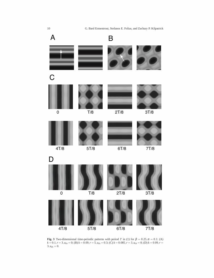
where N1 = |z1|2 + |z3|2 and N2 = |z2|2 + |z4|2. Here, a, . . . ,e are all complexnumbers;a depends only on the linearized equation, whileb, . . . ,e depend onF ′′(0)2,F ′′′(0) and w(x). For the case of no quadratic nonlinearities (ut = 0),b = c = d = e. There are many qualitatively different solutions to this systemwhich correspond to interesting patterns. [47] describe each of them as well astheir conditions for stability. Travelling roll patterns (TR) consist of either hori-zontal or vertical traveling waves that are constant along one direction. They cor-respond to solutions to equation (5) where exactly onezj 6= 0. Standing rolls cor-respond toz1 = z3 6= 0, z2 = z4 = 0. (Note, the contrary case withz1 = z3 = 0andz2 = z4 6= 0 are also standing rolls.) Traveling squares or spots correspond toz1 = z2 6= 0 andz3 = z3 = 0. Standing squares (a blinking checkerboard pattern)correspond toz1 = z2 = z3 = z4 6= 0. A very interesting patern that we see is thealternating roll pattern where horizontal blinking stripes switch to vertical blinkingstripes. These correspond to solutions of the formz1 = −iz2 = z3 = −iz4 6= 0. Fig.3 illustrates the results of simulations of equation (1) on the square doubly periodicdomain in the cse wherem∗ = 2. Thus, all the patterns show two spatial cycles alongthe principle directions. In the simulations illustrated in the figure, we changeuth, rwhich affect the values ofF ′′(0),F ′′′(0) and thus the values of the coefficients ofthe normal form, (5). The relative sizes of these coefficients determin both the am-plitude and the stability of the patterns. Fig. 3A shows the TR solutions foruth = 0(which makesF ′′(0) vanish), while panel B shows a traveling spot pattern. Neitherof these patterns can be simultaneosusly stable. However, there can be other patternsthat stably coexist. Fig. 3C illustrates the “alternating roll” pattern in which there isa switch from vertical to horizontal standing roles. Fig. 3Dshows a pattern thatcombines a standing roll (alternating vertical stripes) with a checkerboard pattern inbetween.

[14] has partially analyzed the more complicated case in which there are 8 crit-ical wave vectors, for examplem∗ =

√5 in Fig. 2. All of the patterns we described

above are also found as solutions to his amplitude equations. In some specific cases,he finds evidence of chaotic behavior. Thus, even near the bifurcation, we can expectthe possibility of complex spatiotemporal dynamics in models like present equa-


D

0

7T/8

T/8 2T/8 3T/8

6T/85T/84T/8

C

4T/8 5T/8 6T/8 7T/8

0 T/8 2T/8 3T/8

BA

Fig. 3 Two-dimensional time-periodic patterns with periodT in (1) for β = 0.25,α = 0.1: (A)k= 0.1, r = 3,uth = 0; (B) k= 0.09, r = 5,uth = 0.3; (C)k= 0.085, r = 3,uth = 0; (D) k= 0.09, r =3,uth = 0.


tions. [50] also considers this case, but only when the quadratic terms (e.g.,F ′′(0))are zero. Obviously, there is a great reduction in the complexity of the patterns andthe resulting possibilites are restricted. Them∗ = 5 case has, to our knowledge, notyet been analyzed.

2.3 Summary of pattern formation.

On a periodic one-dimensional domain, equation (1) can undergo a variety of bifur-cations from the homogeneous state and these can be reduced via the constructionof normal forms to one or two ordinary differential equations for the complex am-plitudes. These bifurcations are generic in the sense that you can expect them tohappen as you vary asingleparameter. If you have the freedom to vary several pa-rameters, then it is possible to arrange them so that multiple instabilities occur atthe same time. For example [19] looked at the Wilson-Cowan neural field equationswhenW(m) =W(m+1) with corresponding imaginary eigenvalues (a double Hopfbifurcation). More recently, [13] studied (1) nearR= 1. WhenR= 1, recall that boththe trace and the determinant vanish at the critical wave number and critical sensi-tivity k. Thus, there is a Bogdanov-Takens bifurcation. The normal form is morecomplicated in this case; however for (1), the only solutions that were found werethe stationary periodic patterns, standing waves, and traveling waves.

In two spatial dimensions, the dynamics is considerably richer due to the fact thatthe symmetry of the square allows for many critical wave vectors becoming unstablesimultaneously. The richness increases with the size of thecritical wavenumber,m∗.As a ballpark estimate, the critical wavenumber is proportional to the ratio of thedomain size and the spatial scale of the connectivity function,w(x). Thus, for, say,global inhibition, the critical wavenumber is close to 1 andthe possible patterns arevery simple. We remark that by estimating the spatial frequency of visual halluci-nations, it is possible to then estimate the characteristiclength scale in visual cortex[5].

3 Response to inputs in the ring network

We now consider the effects of linear adaptation in the ring model [26, 13] in thepresence of external inputs. We show that adaptation usually degrades the ability ofthe network to track input locations. We consider the domainD = (−π ,π) and takew to be the cosine function [26]

w(x− y) = cos(x− y), (1)

so w(x− y) ≷ 0 when |x− y| ≶ π/2. Networks with lateral-inhibitory synapticweights like (1) are known to sustain stable stationary bumps [1, 26, 8, 4]. Many


of our calculations are demonstrated in the case that the firing rate functionf is theHeaviside step function [1, 39, 8, 4]

F(u)≡ H(u−θ ) =

1 : x> θ ,0 : x< θ . (2)

We consider both stationary and propagating inputs with thesimple functional form

I(x, t) = I0cos(x− c0t), (3)

so they are unimodal inx. We study the variety of bifurcations that can arise in thesystem (1) due to the inclusion of adaptation and inputs.

For vanishing adaptation (β → 0), we find stable stationary bumps. For suf-ficiently strong adaptation, the input-free (I0 = 0) network (1) supports travelingbumps (pulses). The network locks to moving inputs as long astheir speed is suffi-ciently close to that of naturally arising traveling bumps.Otherwise, activity period-ically slips off of the stimulus or sloshes about the vicinity of the stimulus location.Previously, Hansel and Sompolinsky [26] studied many of these results, and recently[31] reinterpreted many of these findings in the context of hallucinogen-related vi-sual pathologies.

3.1 Existence of stationary bumps

First, we study existence of stationary bump solutions in the presence of sta-tionary inputs (I(x, t) ≡ I(x))). Assuming stationary solutions(u(x, t),v(x, t)) =(U(x),V(x)) to (1) generates the single equation

(1+β )U(x) =∫ π

−πw(x− y)F(U(y))dy+ I(x). (4)

For a cosine weight kernel (1), we can exploit the trigonometric identity

cos(x− y) = cosycosx+ sinysinx, (5)

and consider the cosine input (3), which we take to be stationary (c0 = 0). Thissuggests looking for even-symmetric solutions

U(x) =

(

A+I0

1+β

)

cosx, (6)

so that the amplitude of (6) is specified by the implicit equation

A=1

1+β

∫ π

−πcosyF((A+(1+β )−1I0)cosy)dy. (7)


For a Heaviside firing rate function (2), we can simplify the implicit equation (7),using the fact that (6) is unimodal and symmetric so thatU(x) > θ for x∈ (−a,a)for solutionsA> 0. First of all, this means that the profile ofU(x) crosses throughthresholdθ at two distinct points [1, 8, 4]

U(±a) = [A+(1+β )−1I0]cosa= θ ⇒ a= cos−1[

(1+β )θ(1+β )A+ I0

]

. (8)

The threshold condition (8) converts the integral equation(7) to

A=1

1+β

∫ a

−acosydy=

21+β

√

1− (1+β )2θ 2

((1+β )A+ I0)2 , (9)

which can be converted to a quartic equation and solved analytically [30].In the limit of no inputI0 → 0, the amplitude of the bump is given by the pair of

real roots of (9)

A± =

√

1+(1+β )θ ±√

1− (1+β )θ1+β

, (10)

so there are two bump solutions. As is usually found in lateral inhibitory neuralfields, the wide bump (+) is stable and the narrow bump (−) is unstable in thelimit of vanishing adaptation (β → 0) [1, 40, 4, 12]. At a criticalβ , the wide bumpundergoes a drift instability leading to a traveling bump.

3.2 Linear stability of stationary bumps

We now compute stability of the bump (6) by studying the evolution of small,smooth, separable perturbations. By pluggingu= U(x)+ψ(x)eλ t andv= V(x)+φ(x)eλ t (where|ψ(x)| ≪ 1 and|φ(x)| ≪ 1) into (1), Taylor expanding, and truncat-ing to first order we find the linear system

(λ +1)ψ(x) =−β φ(x)+∫ π

−πw(x− y)F ′(U(y))ψ(y)dy, (11)

(λ +α)φ(x) = αψ(x). (12)

For the cosine weight function (1), we apply the identity (5)and substitute (12) into(11) to yield the single equation

Q(λ )ψ(x) = (λ +α)(A cosx+B sinx) (13)

whereQ(λ ) = (λ +α)(λ +1)+αβ and

A =

∫ π

−πcosxF′(U(x))ψ(x)dx, B =

∫ π

−πsinxF′(U(x))ψ(x)dx. (14)


We can then plug (13) into the system of equations (14) and simplify to yield

Q(λ )A = (λ +α)

(

∫ π

−πF ′(U(x))dx− (1+β )2A

(1+β )A+ I0

)

A , (15)

Q(λ )B =(λ +α)(1+β )2A(1+β )A+ I0

B, (16)

where we have used the fact that integrating (7) by parts yields

A=A+(1+β )−1I0

1+β

∫ π

−πsin2xF′((A+(1+β )−1I0)cosx)dx,

as well as the fact that the off-diagonal terms vanish, sincetheir integrands are odd.This means that the eigenvalues determining the linear stability of the bump (6)are of two classes: (a) those of even perturbations soψ(x) = cosx and (b) thoseof odd perturbations whereψ(x) = Dφ(x) = sinx. We primarily study eigenvaluesassociated with odd perturbations, given by the quadratic equation

λ 2+[1+α − (1+β )Ω ]λ +α(1+β )(1−Ω) = 0, Ω =(1+β )A

(1+β )A+ I0. (17)

We can use (17) to study two bifurcations of stationary bumpsin the system (1).First, we show a drift instability arises in the input-free (I0 = 0) network, leadingto a pitchfork bifurcation whose resultant attracting solutions are traveling bumps[26, 39, 35, 13, 10]. Second, we show that in the input-drivensystem (I0 > 0), anoscillatory instability arises where the edges of the “slosh” periodically. This is aHopf bifurcation, which also persists for moving inputs (c0 > 0).

In the limit of no input (I0 → 0), Ω → 1, so (17) reduces to

λ 2+[α −β ]λ = 0. (18)

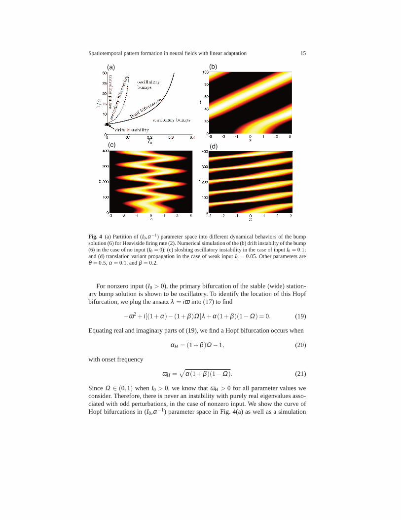
There is always a zero eigenvalue, due to the translation symmetry of the input-free network [1, 40]. Fixing adaptation strengthβ , we can decrease the rateα frominfinity to find the other eigenvalue crosses zero whenα = β . We mark this point inour partition of parameter space into different dynamical behaviors in Fig. 4(a). Thisnon-oscillatory instability results in a traveling bump, indicated by the associatedshift eigenfunction (sinx). Traveling pulses can propagate in either direction, so thefull system (1) undergoes a pitchfork bifurcation. We demonstrate the instabilityresulting in a traveling bump in Fig. 4(b).

We could also ensure that instabilities associated with even perturbations (cosx)of the bump (6) do not occur prior to this loss of instability of the odd perturbation.For brevity, we omit this calculation. Numerical simulations (as shown in Fig. 4(b))verify odd perturbations are the first to destabilize. Therefore, we would alwaysexpect that asα is decreased from infinity, the first instability that arisesis associatedwith odd perturbations of the bump, leading to a drift instability and thus a travelingbump solution (see Fig. 4).


(a) (b)

(c) (d)

Fig. 4 (a) Partition of (I0,α−1) parameter space into different dynamical behaviors of thebumpsolution (6) for Heaviside firing rate (2). Numerical simulation of the (b) drift instabilty of the bump(6) in the case of no input (I0 = 0); (c) sloshing oscillatory instability in the case of input I0 = 0.1;and (d) translation variant propagation in the case of weak input I0 = 0.05. Other parameters areθ = 0.5, α = 0.1, andβ = 0.2.

For nonzero input (I0 > 0), the primary bifurcation of the stable (wide) station-ary bump solution is shown to be oscillatory. To identify thelocation of this Hopfbifurcation, we plug the ansatzλ = iω into (17) to find

−ω2+ i[(1+α)− (1+β )Ω ]λ +α(1+β )(1−Ω) = 0. (19)

Equating real and imaginary parts of (19), we find a Hopf bifurcation occurs when

αH = (1+β )Ω −1, (20)

with onset frequency

ωH =√

α(1+β )(1−Ω). (21)

SinceΩ ∈ (0,1) when I0 > 0, we know thatωH > 0 for all parameter values weconsider. Therefore, there is never an instability with purely real eigenvalues asso-ciated with odd perturbations, in the case of nonzero input.We show the curve ofHopf bifurcations in (I0,α−1) parameter space in Fig. 4(a) as well as a simulation


of the resulting oscillatory solution in Fig. 4(c). Studiesof input-driven excitatorynetworks reveal it is the even mode that destabilizes into oscillations, yielding re-flection symmetric breathers [23, 22]. Here, due to the lateral inhibitory kernel, theodd eigenmode destabilizes, leading to sloshing breathers[22, 42]. As in the caseof the drift instability, we should ensure that instabilities associated with even per-turbations do not arise prior to the Hopf bifurcation. We have ensured this for thecalculations of Fig. 4 but do not show this explicitly here.

Finally, we note a secondary bifurcation which leads to dynamics that evolves asa propagating pattern with varying width (see Fig. 4(d)). Essentially, the “sloshing”bump breaks free from the attraction of the pinning stimulusand begins to prop-agate. As it passes over the location of the stimulus, it expands. Such secondarybifurcations have been observed in adaptive neural fields oninfinite spatial domainstoo [23]. While we cannot develop a linear theory for this bifurcation, we can deter-mine the location of this bifurcation numerically.

3.3 Existence of traveling bumps

Our linear stability analysis of stationary bumps predictsthe existence of travelingbumps for substantially slow and strong adaptation. We can also show that whena moving input is introduced, the system tends to lock to it ifit has speed com-mensurate with that of the natural wave. Converting to a wavecoordinate frameξ = x− c0t where we choose the stimulus speedc0, we can study traveling wavesolutions(u(x, t),v(x, t)) = (U(ξ ),V(ξ )) of (1) with the second order differentialequation [23]

−c20U

′′(ξ )+ c0(1+α)U ′(ξ )−α(1+β )U(ξ ) = G(ξ ) (22)

where

G(ξ ) =(

cd

dξ−α

)[

∫ π

−πw(ξ − y)F(U(y))dy+ I(ξ +∆I )

]

, (23)

and∆I specifies the spatial shift between the moving input and the pulse that tracksit. In the case of a cosine weight kernel (1) and input (3), we can apply the identity(5) to (23) so we may write the equation (22) as

−c20U

′′(ξ )+ c0(1+α)U ′(ξ )−α(1+β )U(ξ ) = C cosξ +S sinξ . (24)

where

C =

∫ π

−πcosx

[

c0F ′(U(x))U ′(x)−αF(U(x))]

dx− I0(α cos∆I + c0sin∆I ), (25)

S =

∫ π

−πsinx

[

c0F ′(U(x)U ′(x)−αF(U(x)))]

dx+ I0(α sin∆I − c0cos∆I ). (26)


By treatingC andS as constants, it is straightforward to solve the second orderdifferential equation (24) to find

U(ξ ) =(c2

0−α −αβ )[C cosξ +S sinξ ]+ c0(1+α)[C sinξ −S cosξ ](c2

0−α(1+β ))2+ c20(1+α)2

. (27)

In the case of a Heaviside firing rate function (2), we can evaluate the integral termsof C andS directly. First, we break the translation symmetry of the system byfixing the threshold crossing points,U(π) =U(π −∆) = θ . This specifies the inputshift parameter∆I as well. We also require that the superthreshold regionU(ξ )> θwhenx∈ (π −∆ ,π) andU(ξ )< θ otherwise. This yields

C = α sin∆ + c0(1− cos∆)− I0(α cos∆I + c0sin∆I ), (28)

S = c0sin∆ −α(1− cos∆)+ I0(α sin∆I − c0cos∆I ). (29)

Plugging this into (27) and imposing threshold conditions,we have the system

X1[sin∆ − I0cos∆I ]−X2[1− cos∆ − I0sin∆I ]

(c20−α(1+β ))2+ c2

0(1+α)2= θ , (30)

X1[sin∆ − I0cos(∆ −∆I )]+X2[1− cos∆ − I0sin(∆ −∆I )]

(c20−α(1+β ))2+ c2

0(1+α)2= θ , (31)

whereX1 = c20+α2(1+β ) andX2 = c3

0+c0α2−c0αβ , which we could solve thenumerically (see [31]).

In the limit of no input (I0 → 0), we can treatc = c0 as an unknown parameter.By taking the difference of (31) and (30) in this limit, we seethat we can computethe speed of natural waves by studying solutions of

c3+ cα2− cαβ = 0, (32)

a cubic equation providing up to three possible speeds for a traveling bump solution.The trivial c = 0 solution is the limiting case of stationary bump solutionsthat wehave already studied and is unstable whenα < β . In line with our bump stabilitypredictions, forα ≤ β , we have the two additional solutionsc± = ±

√

αβ −α2,which provides a right-moving (+) and left-moving (−) traveling bump solution.The pulse widths are then given applying the expression (32)into (30) and (31) andtaking their mean to find sin∆ =(1+α)θ . Thus, we can expect to find four travelingbump solutions, two with each speed, that have widths∆s = π − sin−1[θ (1+α)]and∆u = sin−1[θ (1+α)]. We can find, using linear stability analysis, that the twotraveling bumps associated with the width∆s are stable [35, 39].


(a) (b)

(c) (d)

Fig. 5 Sloshing instability of stimulus-locked traveling bumps (27) in adaptive neural field (1)with Heaviside firing rate (2). (a) Dependence of stimulus locked pulse width∆ on stimulusspeedc0, calculated using the implicit equations (30) and (31). (a)Zeros of the Evans functionE (λ ) = det(Ap− I), with (41), occur at the crossings of the zero contours of ReE (λ ) (black) andImE (λ ) (grey). Presented here for stimulus speedc0 = 0.042, just beyond the Hopf bifurcationat cH ≈ 0.046. Breathing instability occurs in numerical simulations for (b) c0 = 0.036 and (c)c0 = 0.042. (d) When stimulus speedc0 = 0.047 is sufficiently fast, stable traveling bumps lock.Other parameters areθ = 0.5, α = 0.05,β = 0.2, andI0 = 0.1.

3.4 Linear stability of traveling bumps

To analyze the linear stability of stimulus-locked traveling bumps (27), we study theevolution of small, smooth, separable perturbations to (U(ξ ),V(ξ )). To find this, weplug the expansionsu(x, t) =U(ξ )+ψ(ξ )eλ t andv(x, t) =V(ξ )+φ(ξ )eλ t (where|ψ(ξ )| ≪ 1 and|φ(ξ )| ≪ 1) and truncate to first order to find the linear equation[56, 10, 25]

−c0ψ ′(ξ )+ (λ +1)ψ(ξ ) =−β φ(ξ )+∫ π

−πw(ξ − y)F ′(U(y))ψ(y)dy, (33)

−c0φ ′(ξ )+ (λ +α)φ(ξ ) = αψ(ξ ). (34)

For the cosine weight function (1), we can apply the identity(5), so that upon con-verting the system to a second order differential equation,we


−c20ψ ′′+ c(2λ +1+α)ψ ′− [(λ +1)(λ +α)+αβ ]ψ = A cosξ +B sinξ , (35)

where

A =−(λ +α)

∫ π

−πcosξ F ′(U(ξ ))ψ(ξ )dξ + c0

∫ π

−πsinξ F ′(U(ξ ))ψ(ξ )dξ , (36)

B =−c0

∫ π

−πcosξ F ′(U(ξ ))ψ(ξ )dξ − (λ +α)

∫ π

−πsinξ F ′(U(ξ ))ψ(ξ )dξ . (37)

Employing periodic boundary conditionsψ(−π) = ψ(π) andψ ′(−π) = ψ ′(π) andtreatingA andB as constants, it is then straightforward to solve (35) to find

ψ(ξ ) =P2A −P1B

Dpcosξ +

P1A +P2B

Dpsinξ . (38)

whereP1 = c0(2λ +1+α), P2 = c20− [(λ +1)(λ +α)+αβ ], andDp = P2

1 +P2

2 . We can then use self-consistency to determine the constantsA andB, whichimplicitly depend uponψ itself. In the case that the firing rate function is a Heaviside(2), we can reduce this to a pointwise dependence, so that

A =c0sin∆ψ(π −∆)

|U ′(π −∆)| +(λ +α)

[

ψ(π)|U ′(π)| +

cos∆ψ(π −∆)

|U ′(π −∆)|

]

, (39)

B = c0

[

ψ(π)|U ′(π)| +

cos∆ψ(π −∆)

|U ′(π −∆)|

]

− (λ +α)sin∆ψ(π −∆)

|U ′(π −∆)| , (40)

and we can write the solution

ψ(ξ ) =C1cosξ +S1sinξ

Dp

ψ(π)|U ′(π)| +

C2cosξ +S2sinξDp

ψ(π −∆)

|U ′(π −∆)| ,

where

C1 = P2(λ +α)−P1c0, S1 = P1(λ +α)+P2c0,

C2 = P1((λ +α)sin∆ − c0cos∆)+P2(c0sin∆ +(λ +α)cos∆),

S2 = P1((λ +α)cos∆ + c0sin∆)+P2(c0cos∆ − (λ +α)sin∆).

Applying self consistency, we have a 2×2 eigenvalue problemΨ = ApΨ , where

Ψ =

(

ψ(π)ψ(π −∆)

)

, Ap =

(

Aππ Aπ∆A∆π A∆∆

)

, (41)

with

Aππ =− C1

Dp|U ′(π)| , Aπ∆ =− C2

Dp|U ′(π −∆)| ,

A∆π =S1sin∆ −C1cos∆

Dp|U ′(π)| , A∆∆ =S2sin∆ −C2cos∆

Dp|U ′(π −∆)| .


Then, applying the approach of previous stability analysesof traveling waves inneural fields [56, 10, 25], we examine nontrivial solutions of Ψ = ApΨ so thatE (λ ) = 0, whereE (λ ) = det(Ap− I) is called the Evans function of the travelingbump solution (27). Since no other parts of the spectrum contribute to instabilities inthis case, the traveling bump is linearly stable as long as Reλ < 0 for all λ such thatE (λ ) = 0. We can find the zeros of the Evans function by following the approachof [10, 25] and writingλ = ν + iω and plotting the zero contours of ReE (λ ) andIm E (λ ) in the(ν,ω)-plane. The Evans function is zero where the lines intersect.

We present examples of this analysis in Fig. 5. As shown, we can use the im-plicit equations (30) and (31) to compute the width of a stimulus-locked pulse as itdepends upon the speed of the input in the case of a Heaviside firing rate function(2). In parameter regime we show, there are two pulses for each parameter value,either both are unstable or one is stable. As the speed of stimuli is decreased, astable traveling bump undergoes a Hopf bifurcation. For sufficiently fast stimuli, astable traveling bump can lock to the stimulus, as shown in Fig. 5(d). However, forsufficiently, slow stimuli, the speed of natural traveling bumps of the stimulus freenetwork is too fast to track the stimuli. Therefore, an oscillatory instability results.We plot the zeros of the Evans functions associated with thisinstability in Fig. 5(a).The sloshing pulses that result are picture in Fig. 5(b) and (c). Note that, as wasshown in [31], it is possible for pulses to destabilize due tostimuli being too fast.In this context, such an instability occurs through a saddle-node bifurcation, ratherthan a Hopf.

4 Stationary and traveling activity bumps on the infinite line

We consider the neural field (1) in the case of a Heaviside firing rate functionF(u) = H(u−θ ) with firing thresholdθ whereu(x, t) andv(x, t) are defined alongthe infinite line withu(x, t),v(x, t) → 0 asx → ±∞. The synaptic weight functionw is taken to be either excitatory(w(x) > 0) or of Mexican hat form (w(x) locallypositive, laterally negative) and is assumed to satisfyw(x) < w(0) for all x 6= 0 and∫ ∞−∞ w(y)dy< ∞. We considerstationaryactivity bumps in section 4.1 andtraveling

activity bumps in section 4.2 and examine the two cases of (i) bumps generated in-trinsically by the network with no input(I(x, t) = 0) and (ii ) bumps induced by alocalized, excitatory input inhomogeneity(I(x, t) > 0) which can be either station-ary (I(x)) or traveling(I(x− ct)) with constant speedc. The input is assumed tohave an even-symmetric, Gaussian-like profile satisfyingI(x)→ 0 asx→ ±∞.

4.1 Natural and stimulus-induced stationary activity bumps

Existence of stationary bumps.An equilibrium solution of (1) is expressed as(u(x, t),v(x, t))T = (U(x),V(x))T and satisfiesV(x) =U(x) and


1.5 1.5

1.0 1.0

0.5

0 00.5 0.51.0 1.0

0.5

00

0

(a) (b) (c)

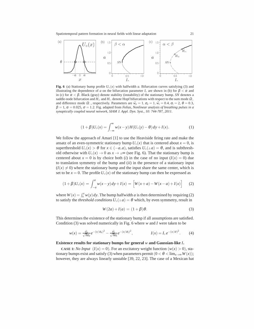
Fig. 6 (a) Stationary bump profileU(x) with halfwidth a. Bifurcation curves satisfying (3) andillustrating the dependence ofa on the bifurcation parameterI are shown in (b) forβ < α andin (c) for α < β . Black (gray) denote stability (instability) of the stationary bump.SN denotes asaddle-node bifurcation andH⊕ andH⊖ denote Hopf bifurcations with respect to the sum modeΩ+

and difference modeΩ−, respectively. Parameters are ¯we = 1, σe = 1, wi = 0.4, σi = 2, θ = 0.3,β = 1, α = 0.025,σ = 1.2. Fig. adapted fromFolias, Nonlinear analysis of breathing pulses in asynaptically coupled neural network, SIAM J. Appl. Dyn. Syst., 10: 744-787, 2011.

(1+β )U(x) =∫ ∞

−∞w(x− y)H(U(y)−θ )dy+ I(x). (1)

We follow the approach of Amari [1] to use the Heaviside firingrate and make theansatz of an even-symmetric stationary bumpU(x) that is centered aboutx= 0, issuperthresholdU(x) > θ for x ∈ (−a,a), satisfiesU(±a) = θ , and is subthresh-old otherwise withU(x) → 0 asx→ ±∞ (see Fig. 6). That the stationary bump iscentered aboutx = 0 is by choice both (i) in the case of no input (I(x) = 0) dueto translation symmetry of the bump and (ii ) in the presence of a stationary input(I(x) 6= 0) where the stationary bump and the input share the same center, which isset to bex= 0. The profileU(x) of the stationary bump can then be expressed as

(1+β )U(x) =∫ a

−aw(x− y)dy+ I(x) =

[

W(x+a)−W(x−a)+ I(x)]

(2)

whereW(x) =∫ x

0 w(y)dy. The bump halfwidtha is then determined by requiring (2)to satisfy thethreshold conditions U(±a) = θ which, by even symmetry, result in

W(2a)+ I(a) = (1+β )θ . (3)

This determines the existence of the stationary bump if all assumptions are satisfied.Condition (3) was solved numerically in Fig. 6 wherew andI were taken to be

w(x) = we√πσe

e−(x/σe)2 − wi√

πσie−(x/σi)

2, I(x) = Ie−(x/σ)2. (4)

Existence results for stationary bumps for generalw and Gaussian-likeI .CASE I: No Input (I(x) = 0). For an excitatory weight function(w(x)> 0), sta-

tionary bumps exist and satisfy (3) when parameters permit(0< θ < limx→∞ W(x));however, they are always linearly unstable [39, 22, 23]. Thecase of a Mexican hat


weight functionw is an extension of the Amari neural field [1] with the existenceequation containing an extra factor due to adaptation(W(2a) = θ (1+ β )); how-ever, the dynamics of the adaptation variablev additionally governs the stability ofthe stationary bump [22]. In particular, ifα < β , stationary bumps are always un-stable. Stable bumps in the scalar model of Amari can extend to this model onlyfor α > β , and a stable bump forα > β destabilizes asα decreases throughα = βleading to a drift instability [22] that can give rise to traveling bumps.

CASE II : Localized Excitatory Input(I(x)> 0). A variety of bifurcation scenar-ios can occur [23, 22], and, importantly, stationary bumps can emerge in a saddle-node bifurcation for strong inputs in parameter regions where stationary bumps donot exist for weak or zero input as shown in Fig. 6. When stationary bumps existfor α > β , the stability of a bump is determined directly by the geometry of thebifurcation curves [22, 23] (e.g., see Fig. 6). Asα decreases throughα = β , a Hopfbifurcation point emerges from a saddle-node bifurcation point (associated with thesum modeΩ+) and destabilizes a segment of a branch of stable bumps forα < β .Generally, Hopf bifurcations occur with respect to either of two spatial modesΩ±(discussed later), and their relative positions (denoted by H⊕ andH⊖, respectively,on the bifurcation curves in Fig. 6) can switch depending on parameters [22].

Stability of stationary bumps. By settingu(x, t)=U(x, t)+ϕ(x, t) andv(x, t)=V(x, t)+ ψ(x, t), we study the evolution of small perturbations(ϕ , ψ)T in a Taylorexpansion of (1) about the stationary bump(U,V)T. To first order in(ϕ , ψ)T, theperturbations are governed by the linearization

∂t ϕ = −ϕ −β ψ +

∫ ∞

−∞w(x− y)H ′(U(y)−θ

)

ϕ(y, t)dy,

1α ∂t ψ = +ϕ − ψ.

(5)

Separating variables, we setϕ(x, t) = eλ tϕ(x) andψ(x, t) = eλ tψ(x) in (5) where(ϕ ,ψ)T ∈ C1

u(R,C2) denoting uniformly continuously differentiable vector-valued

functionsu : R−→C2. This leads to the spectral problem forλ and(ϕ ,ψ)T

M

(

ϕψ

)

= λ(

ϕψ

)

, M

(

ϕψ

)

=

[

−1 −βα −α

](

ϕψ

)

+

(

Nϕ0

)

, (6)

whereNϕ(x) =∫ ∞−∞ w(x− y)H ′(U(y)−θ )ϕ(y)dy. The essential spectrum lies in

the left-half complex plane and plays no role in instability[23, 22]. To calculate thepoint spectrum, defineρ(λ ) = λ +1+

αβλ+α and reduce (6) toψ(x) =

( αλ+α

)

ϕ(x) and

ρ(λ )ϕ(x) =w(

x−a)

|U ′(+a)| ϕ(a) +w(

x+a)

|U ′(−a)| ϕ(−a). (7)

Settingx= ±a in (7) yields a compatibility condition for the values ofϕ(±a) where

(

Λ−ρ(λ ) I)

(

ϕ(+a)ϕ(−a)

)

= 0, Λ = 1|U ′(a)|

[

w(0) w(2a)w(2a) w(0)

]

.


Consequently, nontrivial solutions of (6) exist whendet(Λ−ρ(λ )I) = 0, therebyidentifying eigenvaluesλ . The point spectrum comprises two pairs of eigenvaluesλ+±, λ−

± and eigenfunctionsv+±,v

−± defining two characteristic spatial modes [22, 23]:

Sum mode– eigenvaluesλ+

± and eigenvectorsv+±(x) = Ω+(x)(λ+

±+ α,α)T,

λ+

±(a) =− 12ϒ+± 1

2

√

ϒ 2+ −4Γ+ , Ω+(x) = w(x−a)+w(x+a),

Difference mode– eigenvaluesλ−± and eigenvectorsv−

±(x) = Ω−(x)(λ−±+ α,α

)T,

λ−±(a) =− 1

2ϒ−± 12

√

ϒ 2− −4Γ− , Ω−(x) = w(x−a)−w(x+a),

whereΩ+(x) is even-symmetric,Ω−(x) is odd-symmetric, andϒ±,Γ± are given by

ϒ±(a) = (1+α)− (1+β )Ω±(a)|U ′(a)|

, Γ±(a) = α (1+β )[

1− Ω±(a)|U ′(a)|

]

.

Stability results for stationary bumps for general w and Gaussian-likeI .CASE I: No Input (I(x) = 0) [23, 25, 41, 22]. With no input,|U ′

(a)| = Ω−(a)and the eigenvaluesλ−

± can be redefined asλ−+ ≡ 0 andλ−

− = β −α. In this case,the persistent 0-eigenvalueλ−

+ ≡ 0 corresponds to the translation invariance of thestationary bump and is associated with an eigenfunction in the difference modeΩ−. The other eigenfunction in the difference mode (associated with λ−

−) is stablefor β < α and unstable forα < β . Thus, forα < β , a stationary bump is alwayslinearly unstable. Forβ < α, a stationary bump can be linearly stable for a Mexicanhat weight function (ifw(2a) < 0) but is always unstable for an excitatory weightfunction (w(x) > 0) [22]. Also, forβ < α, it is not possible for a stationary bumpto undergo a Hopf bifurcation and, asβ is increased throughα, a stable stationarybump undergoes a drift instability due to eigenvalueλ−

− increasing through 0 [22].Interestingly, multibump solutions in (1) on two-dimensional domains are capableof undergoing a bifurcation to a rotating traveling multibump solution [37].

CASE II : Localized Excitatory Input(I(x)> 0) [7, 23, 22]. The presence of theinput inhomogeneity (I(x) 6= 0) breaks translation symmetry andλ−

+ 6= 0 generically.A stationary bump is linearly stable whenλ+

±,λ−± < 0 which reduce to the conditions

Ω+(a)|U ′(a)|

< 1 if α > β , andΩ±(a)|U ′(a)|

<1+α1+β

if α < β .

If w(0) > w(x) for all x 6= 0, (2) implies(1+β )|U ′(a)| = w(0)−w(2a)+ |I ′(a)|.

Consequently, the stability conditions translate, in terms of the gradient|I ′(a)|, to

α > β :∣

∣I ′(a)∣

∣ > DSN(a)≡ 2w(2a),

α < β :∣

∣I ′(a)∣

∣ > DH(a)≡

(β−α1+α

)

Ω+(a)+2w(2a), w(2a)> 0,(β−α

1+α)

Ω−(a), w(2a)< 0.


Fig. 7 Destabilization of spatial modesΩ+(x) andΩ−(x), as the bifurcation parameterI is variedthrough a Hopf bifurcation, can give rise to a stablebreatheror slosher, respectively, dependingon the relative position of the bifurcation point for each spatial mode (e.g.,H⊕ and H⊖ in Fig.6(c)). (a) plot ofu(x, t) for a breather arising from destabilization of the sum modeΩ+(x) forparametersI = 1.9, wi = 0,β = 2.75,α = 0.1,θ = 0.357. (b) plot of u(x, t) for a slosher arisingfrom destabilization of the difference modeΩ−(x) for parametersI = 1.5, wi = 0.4,σi = 2,β =2.6,α = 0.01,θ = 0.35. Common parameters:σ = 1.2, we = 1,σe = 1.

|I ′(a)|=DSN(a) denotes a saddle-note bifurcation point and|I ′(a)|= DH(a) denotesa Hopf bifurcation where a pair of complex eigenvalues associated with one of thetwo spatial modesΩ± crosses into the right-half plane. Ifw(2a) > 0 at the Hopfbifurcation point, the sum modeΩ+ destabilizes and gives rise to abreather—atime-periodic, localized bump-like solution that expandsand contracts. Ifw(2a)< 0at the Hopf bifurcation point, the difference modeΩ− destabilizes and gives rise toa slosher—a time-periodic localized solution that instead sloshes side-to-side asshown in Fig. 7. Nonlinear analysis of the Hopf bifurcation reveals that, to firstorder, the breather and slosher are time-periodic modulations of the stationary bumpU(x) based upon the even and odd geometry of the sum and differencemodes,respectively [22]. Sloshers were also found to occur in [26]. The bifurcation canbe super/subcritical, which can be determined from the normal form or amplitudeequation derived in [22]. Stimulus-induced breathers can undergo further transitionsand can exhibit mode-locking between breathing and emission of traveling bumps(when supported by the network) [23, 25]. Alternatively, breathing fronts can occurfor step function inhomogeneitiesI(x) [7, 6]. Hopf bifurcation of radially symmetricstationary bumps extends to (1) on two-dimensional domains, leading to a varietyof localized time-periodic solutions including nonradially symmetric structures [23,24].


4.2 Natural and stimulus-locked traveling activity bumps

Existence of traveling bumps.We simultaneously consider the two cases ofnaturaltraveling bumps(I(x, t) = 0) andstimulus-lockedtraveling bumps which are lockedto a stimulusI(x− ct) traveling with constant speedc. Natural traveling bumps inneural field (1) on the infinite lineD= (−∞,∞) were first considered in [38, 39] andcan occur in the absence of an input or in a region of the neuralmedium where aninput is effectively zero. An important distinction between the two cases is that thenatural traveling bump in the absence of the input is translationally invariant and wehave stability with respect to a family of translates, whereas in the stimulus-lockedcase there is a fixed position of the bump relative to the input.

Assumeu(x, t) = U(x− ct) andv(x, t) = V(x− ct) and, in traveling wave coor-dinatesξ = x− ct, make the assumption that the activityU(ξ ) is superthresholdU(ξ )> θ for ξ ∈ (ξ1,ξ2), satisfiesU(ξ1,2) = θ , and is substhreshold otherwise withU(ξ )→ 0 asξ → ±∞. Consequently, the profile of the bump satisfies

−cUξ =−U −βV+

∫ ∞

−∞w(ξ −η)H(U(η)−θ )dη + I(ξ ),

− cα

Vξ =+U − V.(8)

Variation of parameters [55, 25] can be used to solve (8) to construct the profile(Uc,Vc)

T of the traveling bump which can be expressed as [25]

Uc(ξ ) = (1− µ−)M+(ξ ) − (1− µ+)M−(ξ )

Vc(ξ ) = −α[

M+(ξ ) −M−(ξ )]

.

wherem(ξ ) =W(ξ − ξ1)−W(ξ − ξ2)+ I(ξ ),

M±(ξ ) =1

c(µ+−µ−)

∫ ∞

ξe

µ±c (ξ−η)m(η)dη , µ± = 1

2

(

1+α ±√

(1−α)2−4αβ)

.

and 0< Reµ− ≤ Reµ+. Sincem(ξ ) is dependent uponξ1,ξ2, the threshold condi-tionsUc(ξi) = θ , wherei = 1,2 andξ1 < ξ2, determine the relationship between theinput strengthI and the position of the bump relative to the inputI(ξ ). This resultsin consistency conditions for the existence of a stimulus-locked traveling bump:

θ = (1− µ−)M+(ξ1) − (1− µ+)M−(ξ1),

θ = (1− µ−)M+(ξ2) − (1− µ+)M−(ξ2).

These determine the existence of the traveling bump (provided the profile satisfiesthe assumed threshold conditions) and include the case of natural waves (I = 0).Note that existence equations for the traveling bump in (8) can also be derived usinga second orderODE forumlation [39, 23] or an integral formulation in [9].


Existence conditions for a positive, exponentialw and GaussianI . For explicitcalculations in this section,w andI are taken to be

w(x) = we2σe

e−|x|/σe, I(x− ct) = Ie−((x−ct)/σ)2. (9)

CASE I: Natural traveling bump(I(ξ ) = 0) with speed c[25, 41, 23, 9, 39]. Inthe absence of an input, translation invariance of the bump allows the simplification(ξ1,ξ2) = (0,a) where the wave speedc and bump widtha are naturally selected bythe network according to the following threshold conditions [25]

θ = J+(−a), θ = K(−a), (10)

whereK(ζ ) = J−(ζ )−H+(ζ )+H−(ζ ), and, forw given in (9),

J±(ζ ) =(α ± c)

(

1−eζ)

(c+ µ+)(c+ µ−), H±(ζ ) =

c2(1− µ∓)(

1−eµ±c ζ )

µ±(c2− µ2±)(µ+−µ−)

. (11)

Note that(c+ µ+)(c+ µ−) = c2 + c(1+α)+α(1+β ). Existence equations (10)were solved numerically in Fig. 8(b) indicating two branches of traveling bumpsfor small α. The wide, faster bump is found to be stable and the narrow, slowerbump is unstable. Detailed analyses of the existence of natural traveling bumps canbe found in [52, 41], including the case where the homogeneous state has complexeigenvalues [52]. A singular perturbation construction for the pulse was carried outfor smooth smooth firing rate functionsF in [39]. For moderate values ofβ trav-eling fronts occur in (1) and were shown to undergo a front bifurcation as a cuspbifurcation with respect to the wave speed of the front [6].

CASE II : Stimulus-locked traveling bump(I(ξ ) 6= 0) with speed c[25]. The waveand stimulus speedsc are identical, and the threshold conditions for(ξ1,ξ2) are [25]

θ = K(ξ1− ξ2) + T+(ξ1)−T−(ξ1),

θ = J+(ξ1− ξ2) + T+(ξ2)−T−(ξ2),(12)

whereK,J+ are given in (11) andT± arises from the input and is given by

T±(ζ ) =√

π σ I2 c

(

1− µ∓

µ+− µ−

)

exp(µ±ζ

c+[µ±σ

2c

]2)

erfc( ζ

σ+

µ±σ2c

)

,

with erfc(z) denoting the complementary error function. (12) can be solved numer-ically to determine the regions of existence of stimulus-locked traveling bumps asboth the speedc and amplitudeI are varied (assumingUc(ξ ) satisfies the thresholdassumptions). This allows us to connect the stationary bumps to natural travelingbumps via stimulus-locked traveling bumps as shown in Fig. 8. This analysis forstimulus-locked fronts was carried out in [6] and an extension of stimulus-lockedbumps for a general smooth firing rate functionF was studied in [20].


00

0 10

20

30

0.02 0.04 0.06

00

0.4

0.8

0.02 0.04

00

1

2

3

0.4 0.8 1.2

s

u

s

(a) (b) (c)

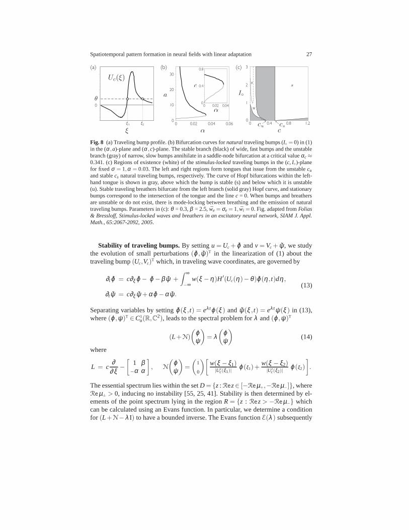
Fig. 8 (a) Traveling bump profile. (b) Bifurcation curves fornatural traveling bumps (I = 0) in (1)in the (α ,a)-plane and (α ,c)-plane. The stable branch (black) of wide, fast bumps and the unstablebranch (gray) of narrow, slow bumps annihilate in a saddle-node bifurcation at a critical valueαc ≈0.341. (c) Regions of existence (white) of thestimulus-lockedtraveling bumps in the (c, I)-planefor fixed σ = 1,α = 0.03. The left and right regions form tongues that issue from the unstablecu

and stablecs natural traveling bumps, respectively. The curve of Hopf bifurcations within the left-hand tongue is shown in gray, above which the bump is stable (s) and below which it is unstable(u). Stable traveling breathers bifurcate from the left branch (solid gray) Hopf curve, and stationarybumps correspond to the intersection of the tongue and the linec = 0. When bumps and breathersare unstable or do not exist, there is mode-locking between breathing and the emission of naturaltraveling bumps. Parameters in (c):θ = 0.3,β = 2.5,we = σe= 1, wi = 0. Fig. adapted fromFolias& Bressloff, Stimulus-locked waves and breathers in an excitatory neural network, SIAM J. Appl.Math., 65:2067-2092, 2005.

Stability of traveling bumps. By settingu= Uc + ϕ andv= Vc + ψ, we studythe evolution of small perturbations(ϕ , ψ)T in the linearization of (1) about thetraveling bump(Uc,Vc)

T which, in traveling wave coordinates, are governed by

∂t ϕ = c∂ξ ϕ − ϕ −β ψ +

∫ ∞

−∞w(ξ −η)H ′(Uc(η)−θ )ϕ(η , t)dη ,

∂tψ = c∂ξ ψ +αϕ −αψ.

(13)

Separating variables by settingϕ(ξ , t) = eλ tϕ(ξ ) andψ(ξ , t) = eλ tψ(ξ ) in (13),where(ϕ ,ψ)T ∈C1

u(R,C2), leads to the spectral problem forλ and(ϕ ,ψ)T

(L+N)

(

ϕψ

)

= λ(

ϕψ

)

(14)

where

L = c∂

∂ξ−[

1 β−α α

]

, N

(

ϕψ

)

=

(

1

0

)[

w(ξ − ξ1)|U ′

c(ξ1)|ϕ(ξ1)+

w(ξ − ξ2)|U ′

c(ξ2)|ϕ(ξ2)

]

.

The essential spectrum lies within the setD= z:Rez∈ [−Reµ+,−Reµ−], whereReµ± > 0, inducing no instability [55, 25, 41]. Stability is then determined by el-ements of the point spectrum lying in the regionR= z : Rez> −Reµ− whichcan be calculated using an Evans function. In particular, wedetermine a conditionfor (L+N−λ I) to have a bounded inverse. The Evans functionE(λ ) subsequently


arises from the condition that(L+N−λ I) is not invertible and(L+N−λ I) = 0has nontrivial solutions. We setu= (ϕ ,ψ)T and use variation of parameters [55, 25]to construct a bounded inverse for(L+N−λ I) based on the integral kernel

M(ξ ,η ,λ ) = 1cβ (µ+−µ−)

[

Φ+(ξ )∣

∣Φ−(ξ )][

Ψ+(η)∣

∣Ψ−(η)]T

(15)

where[A|B] denotes the matrix with column vectors A and B, respectively, and

Φ±(ξ ) =(

βµ±−1

)

e(

λ+µ±c

)

ξ , Ψ±(ξ ) =±(

1−µ∓β

)

e−(

λ+µ±c

)

ξ .

ForRe(λ )>−µ−, we can express(L+N−λ I)u =−f, wheref = ( f1, f2)T, as

u(ξ )−∫ ∞

ξM(ξ ,η ,λ )Nu(η)dη =

∫ ∞

ξM(ξ ,η ,λ )f(η)dη . (16)

From (16),ψ is calculated in terms ofϕ(ξ1), ϕ(ξ2), F2, andλ ,ϕ are determined by

ϕ(ξ )−Λ1(λ ,ξ )ϕ(ξ1)−Λ2(λ ,ξ )ϕ(ξ2) = F1(ξ ) (17)

where M11 denotes the(1,1) entry of M in (15) andi = 1,2 in the expression below

Λi(λ ,ξ ) =∫ ∞

ξM 11(ξ ,η ,λ )

w(η − ξi)

|U ′c(ξi)|

dη ,(

F1(ξ )

F2(ξ )

)

=

∫ ∞

ξM(ξ ,η ,λ ) f(η) dη .

By the Holder inequality,Λi andF1,2 are bounded for allξ ∈R andf ∈C0u(R,C

2). Acompatibility condition that determines the values ofϕ(ξ1) andϕ(ξ2) is producedby substitutingξ = ξ1 andξ = ξ2 into (17) to obtain the matrix equation

(

I −Λ(λ ))(

ϕ(ξ1)ϕ(ξ2)

)

=

(

F1(ξ1)F1(ξ2)

)

, Λ(λ ) =

[

Λ1(λ ,ξ1) Λ2(λ ,ξ1)

Λ1(λ ,ξ2) Λ2(λ ,ξ2)

]

which has a unique solution if and only ifdet(I−Λ(λ )) 6= 0, resulting in a boundedinverse(L+N−λ I)−1 defined on all ofC0

u(R,C2). Conversely, we cannot invert the

operator forλ such thatdet(I −Λ(λ )) = 0, in which case(L+N− λ )u = 0 hasnontrivial solutions corresponding to eigenvaluesλ and eigenfunctions(ϕ ,ψ)T inthe point spectrum. Thus, forRe(λ )>−µ−, we can express the Evans function as

E(λ ) = det(

I −Λ(λ ))

, Re (λ )>−µ−, (18)

which has eigenvaluesλ given by its zero set.Evans function for an exponential weightw and Gaussian-like input I . The

following gives an explicit construction of the Evans function for both natural trav-eling bumps(I = 0) and stimulus-locked bumps(I > 0) in (1) with a Heavsidefiring rate function, exponential weight distribution and Gaussian input given in (9).ForRe(λ )>−µ−, the Evans functionE(λ ) is given by [25]


E(λ ) =[

1− Θ+(λ )|U ′

c(ξ1)|

][

1− Θ+(λ )|U ′

c(ξ2)|

]

− Θ+(λ )Ξ(λ ,ξ1 − ξ2)

|U ′c(ξ1)U ′

c(ξ2)∣

∣

,

where

Γ±(λ ) =(1− µ∓)c

(µ+−µ−)(c2− (λ + µ±)2), Θ±(λ ) =

λ +α ± c2(λ + µ+± c)(λ + µ−± c)

,

Ξ(λ ,ζ ) =Θ−(λ )e2ζ +Γ+(λ )e

[

λ+µ++cc

]

ζ −Γ−(λ )e

[

λ+µ−+cc

]

ζ.

For the case of natural waves whereI = 0, translation invariance allows us to set(ξ1,ξ2) = (0,a). Since the zero set of the Evans functionE(λ ) comprises solutionsof a transcendental equation, the eigenvaluesλ can be determined numerically byfinding the intersection points of the zero sets of the real and complex parts of theEvans function which was used to determined the stability results in Fig. 8. Hopfbifurcations, identified by complex conjugate eigenvaluescrossing the imaginaryaxis, can give rise to traveling breathers or mode-locking between breathing and theemission of natural traveling bumps [25].

For various treatments of the stability of natural traveling bumps and Evans func-tions in (1) see [55, 10, 25, 41, 44, 4], and a comparison between different ap-proaches is found in [44]. Zhang developed the Evans function and analyzed thestability of traveling bumps in the singularly perturbed case 0<α ≪ 1 [55]. Finally,on one-dimensional domains, traveling multibump waves were studied in [52], andtraveling waves have been extended to the case of inhomogeneous synaptic cou-pling in [32] and asymmetric coupling [51]. On two-dimensional domains, spiralwaves [34, 52], traveling and rotating multibumps [37], andthe collision of travel-ing bumps [36] have also been examined.

References

1. S. AMARI , Dynamics of pattern formation in lateral-inhibition type neural fields, Biol. Cy-bern., 27 (1977), pp. 77–87.

2. J. BENDA AND A. V. M. H ERZ, A universal model for spike-frequency adaptation, NeuralComput., 15 (2003), pp. 2523–2564.

3. V. A. BILLOCK AND B. H. TSOU, Elementary visual hallucinations and their relationshipsto neural pattern-forming mechanisms., Psychological Bulletin, (2012).

4. P. C. BRESSLOFF, Spatiotemporal dynamics of continuum neural fields, J Phys. A: Math.Theor., 45 (2012), p. 033001.

5. P. C. BRESSLOFF, J. D. COWAN, M. GOLUBITSKY, P. J. THOMAS, AND M. C. WIENER,Geometric visual hallucinations, euclidean symmetry and the functional architecture of striatecortex, Philos. Trans. Roy. Soc. B., 356 (2001), pp. 299–330.

6. P. C. BRESSLOFF ANDS. E. FOLIAS, Front bifurcations in an excitatory neural network.,SIAM J. Appl Math, 65 (2004), pp. 131–151.

7. P. C. BRESSLOFF, S. E. FOLIAS, A. PRAT, AND Y.-X. L I, Oscillatory waves in inhomoge-neous neural media, Phys Rev Lett, 91 (2003), p. 178101.

8. S. COOMBES, Waves, bumps, and patterns in neural field theories, Biol. Cybern., 93 (2005),pp. 91–108.


9. S. COOMBES, G. J. LORD, AND M. R. OWEN, Waves and bumps in neuronal networks withaxo–dendritic synaptic interactions, Physica D, 178 (2003), pp. 219–241.

10. S. COOMBES AND M. R. OWEN, Evans functions for integral neural field equations withheaviside firing rate function, SIAM J Appl. Dyn. Syst., 3 (2004), pp. 574–600.

11. , Bumps, breathers, and waves in a neural network with spike frequency adaptation,Phys Rev Lett, 94 (2005), p. 148102.

12. S. COOMBES, H. SCHMIDT, AND I. BOJAK, Interface dynamics in planar neural field mod-els, J Math. Neurosci., 2 (2012).

13. R. CURTU AND B. ERMENTROUT,Pattern formation in a network of excitatory and inhibitorycells with adaptation, SIAM J. Appl. Dyn. Syst., 3 (2004), pp. 191–231.

14. J. H. P. DAWES, Hopf bifurcation on a square superlattice, Nonlinearity, 14 (2001), p. 491.15. B. DIONNE, M. SILBER, AND A. C. SKELDON,Stability results for steady, spatially periodic

planforms, Nonlinearity, 10 (1997), p. 321.16. B. ERMENTROUT, Stripes or spots? nonlinear effects in bifurcation of reaction-diffusion

equations on the square, Proceedings of the Royal Society of London. Series A: Mathematicaland Physical Sciences, 434 (1991), pp. 413–417.

17. B. ERMENTROUT, Neural networks as spatio-temporal pattern-forming systems, Rep. Prog.Phys., 61 (1998), pp. 353–430.

18. G. B. ERMENTROUT AND J. D. COWAN, A mathematical theory of visual hallucination pat-terns, Biol. Cybern., 34 (1979), pp. 137–150.

19. , Secondary bifurcation in neuronal nets, SIAM Journal on Applied Mathematics,(1980), pp. 323–340.

20. G. B. ERMENTROUT, J. Z. JALICS, AND J. E. RUBIN, Stimulus-driven traveling solutions incontinuum neuronal models with a general smooth firing rate function, SIAM J. Appl Math,70 (2010), pp. 3039–3064.

21. G. B. ERMENTROUT AND J. B. MCLEOD, Existence and uniqueness of travelling waves fora neural network, Proc. Roy. Soc. Edin., 123A (1993), pp. 461–478.

22. S. E. FOLIAS, Nonlinear analysis of breathing pulses in a synaptically coupled neural net-work, SIAM J. Appl. Dyn. Syst., 10 (2011), pp. 744–787.

23. S. E. FOLIAS AND P. C. BRESSLOFF, Breathing pulses in an excitatory neural network,SIAM J Appl. Dyn. Syst., 3 (2004), pp. 378–407.

24. , Breathers in two-dimensional neural media, Phys Rev Lett, 95 (2005), p. 208107.25. , Stimulus-locked traveling waves and breathers in an excitatory neural network, SIAM

J Appl Math, 65 (2005), pp. 2067–2092.26. D. HANSEL AND H. SOMPOLINSKY,Modeling feature selectivity in local cortical circuits, in

Methods in neuronal modeling: From ions to networks, C. Kochand I. Segev, eds., Cambridge:MIT, 1998, ch. 13, pp. 499–567.

27. X. HUANG, W. C. TROY, Q. YANG, H. MA , C. R. LAING , S. J. SCHIFF, AND J.-Y. WU,Spiral waves in disinhibited mammalian neocortex, J Neurosci., 24 (2004), pp. 9897–9902.

28. V. ITSKOV, C. CURTO, E. PASTALKOVA , AND G. BUZSAKI ,Cell assembly sequences arisingfrom spike threshold adaptation keep track of time in the hippocampus, J. Neurosci., 31 (2011),pp. 2828–2834.

29. Z. P. KILPATRICK AND P. C. BRESSLOFF, Stability of bumps in piecewise smooth neuralfields with nonlinear adaptation, Physica D, 239 (2010), pp. 1048 – 1060.

30. Z. P. KILPATRICK AND B. ERMENTROUT, Wandering bumps in stochastic neural fields,arXiv, (2012).

31. Z. P. KILPATRICK AND G. B. ERMENTROUT, Hallucinogen persisting perception disorderin neuronal networks with adaptation, J Comput Neurosci, 32 (2012), pp. 25–53.

32. Z. P. KILPATRICK , S. E. FOLIAS, AND P. C. BRESSLOFF, Traveling pulses and wave prop-agation failure in inhomogeneous neural media, SIAM J Appl. Dyn. Syst., 7 (2008), pp. 161–185.

33. H. KLUVER, Mescal and the Mechanisms of hallucinations, University of Chicago, 1966.34. C. R. LAING, Spiral waves in nonlocal equations, SIAM J. Appl. Dyn. Syst., 4 (2005),

pp. 588–606.


35. C. R. LAING AND A. L ONGTIN, Noise-induced stabilization of bumps in systems with long-range spatial coupling, Physica D, 160 (2001), pp. 149 – 172.

36. Y. LU, Y. SATO, AND S.-I. AMARI , Traveling bumps and their collisions in a two-dimensional neural field, Neural Comput., 23 (2011), pp. 1248–60.

37. M. R. OWEN, C. R. LAING , AND S. COOMBES, Bumps and rings in a two-dimensionalneural field: splitting and rotational instabilities, New Journal of Physics, 9 (2007), p. 378.

38. D. J. PINTO, Computational, experimental, and analytical explorations of neuronal circuitsin the cerebral cortex, PhD thesis, Department of Mathematics, University of Pittsburgh, Pitts-burgh, PA, 1997.

39. D. J. PINTO AND G. B. ERMENTROUT, Spatially structured activity in synaptically coupledneuronal networks: I. Traveling fronts and pulses, SIAM J Appl. Math., 62 (2001), pp. 206–225.

40. , Spatially structured activity in synaptically coupled neuronal networks: Ii. lateralinhibition and standing pulses, SIAM J. Appl Math, 62 (2001), pp. 226–243.

41. D. J. PINTO, R. K. JACKSON, AND C. E. WAYNE, Existence and stability of traveling pulsesin a continuous neuronal network, SIAM J. Appl. Dyn. Syst., 4 (2005), pp. 954–984.

42. J. RANKIN , E. TLAPALE , R. VELTZ, O. FAUGERAS, AND P. KORNPROBST, Bifurcationanalysis applied to a model of motion integration with a multistable stimulus, Inria: ResearchReport, (2011).

43. M. RULE, M. STOFFREGEN, AND B. ERMENTROUT, A model for the origin and propertiesof flicker-induced geometric phosphenes, PLoS computational biology, 7 (2011), p. e1002158.

44. B. SANDSTEDE, Evans functions and nonlinear stability of traveling wavesin neuronal net-work models., Internat. J. Bifur. Chaos Appl. Sci. Engrg., 17 (2007), pp.2693–2704.

45. E. SCHWARTZ, Spatial mapping in the primate sensory projection: Analytic structure andrelevance to projection, Biol. Cybern., 25 (1977).

46. V. SHUSTERMAN AND W. C. TROY, From baseline to epileptiform activity: a path to syn-chronized rhythmicity in large–scale neural networks, Phys. Rev. E, 77 (2008), p. 061911.

47. M. SILBER AND E. KNOBLOCH,Hopf bifurcation on a square lattice, Nonlinearity, 4 (1991),p. 1063.

48. M. STOCKER, M. KRAUSE, AND P. PEDARZANI, An apamin-sensitiveCa2+–activatedK+

current in hippocampal pyramidal neurons, Proc. Natl. Acad. Sci. USA, 96 (1999), pp. 4662–4667.

49. P. TASS, Cortical pattern formation during visual hallucinations, J. Biol. Phys., 21 (1995),pp. 177–210.

50. , Oscillatory cortical activity during visual hallucinations, J. Biol. Phys., 23 (1997),pp. 21–66.

51. W. C. TROY, Traveling waves and synchrony in an excitable large-scale neuronal networkwith asymmetric connections, SIAM J. Appl. Dyn. Syst., 7 (2008), pp. 1247–1282.

52. W. C. TROY AND V. SHUSTERMAN, Patterns and features of families of traveling waves inlarge-scale neuronal networks, SIAM J. Appl. Dyn. Syst., 6 (2007), pp. 263–292.

53. J.-Y. WU, Propagating waves of activity in the neocortex: What they are, what they do, Neu-roscientist, 14 (2008), pp. 487–502.

54. K. ZHANG, Representation of spatial orientation by the intrinsic dynamics of the head-direction cell ensemble: a theory, J. Neurosci., 16 (1996), pp. 2112–2126.

55. L. ZHANG, On stability of traveling wave solutions in synaptically coupled neuronal net-works., Differential and Integral Equations, 16 (2003), pp. 513–536.

56. L. ZHANG, Existence, uniqueness and exponential stability of traveling wave solutions ofsome integral differential equations arising from neuronal networks, J. Differ. Equations, 197(2004), pp. 162–196.

spatiotemporal pattern formation in neural ﬁelds with...

Documents