spatio-temporal network databases and routing algorithms ... · spatio-temporal network databases...

Spatio-temporal Network Databases andRouting Algorithms: A Summary of Results

Betsy George�, Sangho Kim, and Shashi Shekhar

Department of Computer Science and Engineering, University of Minnesota200 Union St SE, Minneapolis, MN 55455, USA

{bgeorge,sangho,shekhar}@cs.umn.eduhttp://www.spatial.cs.umn.edu/

Abstract. Spatio-temporal networks are spatial networks whose topol-ogy and parameters change with time. These networks are important dueto many critical applications such as emergency traffic planning and routefinding services and there is an immediate need for models that supportthe design of efficient algorithms for computing the frequent queries onsuch networks. This problem is challenging due to potentially conflictingrequirements of model simplicity and support for efficient algorithms.Time expanded networks which have been used to model dynamic net-works employ replication of the network across time instants, resultingin high storage overhead and algorithms that are computationally ex-pensive. In contrast, proposed time-aggregated graphs do not replicatenodes and edges across time; rather they allow the properties of edges andnodes to be modeled as a time series. Since the model does not replicatethe entire graph for every instant of time, it uses less memory and thealgorithms for common operations (e.g. connectivity, shortest path) arecomputationally more efficient than those for time expanded networks.One important query on spatio-temporal networks is the computation ofshortest paths. Shortest paths can be computed either for a given starttime or to find the start time and the path that leads to least traveltime journeys (best start time journeys). Developing efficient algorithmsfor computing shortest paths in a time varying spatial network is chal-lenging because these journeys do not always display greedy propertyor optimal substructure, making techniques like dynamic programminginapplicable. In this paper, we propose algorithms for shortest path com-putations in both contexts. We present the analytical cost models for thealgorithms and provide an experimental comparison of performance withexisting algorithms.

Keywords: time-aggregated graphs, shortest paths, spatio-temporaldata bases.

1 Introduction

The underlying data of interest for many significant applications such as trans-portation networks is structured as a spatio-temporal network, which consists� Corresponding author.

D. Papadias, D. Zhang, and G. Kollios (Eds.): SSTD 2007, LNCS 4605, pp. 460–477, 2007.c© Springer-Verlag Berlin Heidelberg 2007

Spatio-temporal Network Databases and Routing Algorithms 461

of a finite collection of points (i.e. nodes) with location information, the line-segments (i.e. edges) connecting the points, and the time-varying attributes at-tached to the elements. For example, a spatio-temporal network database for atraveler’s trip planning may store the intersections as nodes, the road segmentsas edges, and time dependent travel time attached to the road segments. In thecase of evacuation planning, time dependent capacity may be added to the roadsegments as another important attribute.

Related work in the field of databases falls into three broad categories (1)Spa-tial network databases, (2) Graph Databases, and (3) Spatio-temporal databases.The recent release of Oracle (version 10g) includes a network data model tostore and maintain the connectivity of link-node networks and supports basicfeatures such as shortest path [14]. The Network Analyst extension of ArcMapfrom ESRI supports a network geodatabase and provides basic algorithms (e.g.,shortest path, service area, closest facility, etc.) [7]. However, these products donot address the time variance of spatial networks, which is crucial in applicationssuch as route computations and emergency planning.

Graph databases [5,6,7,19,22,24] also primarily deal with spatial networksthat do not vary with time. Research in graph databases that accounts for tem-poral variations perform computations over a snapshot of the network [4,9,18],and does not consider the interplay between the edge travel times and the ex-istence of edges. For example, Ding [4] proposed a model that addresses thetime-dependency by associating a temporal attribute to every edge and node ofthe network so that its state at any instant of time can be retrieved. This modelperforms path computations over a snapshot of the network. Since the networkcan change over the time taken to traverse these paths, this computation mightnot give realistic solutions. The model does not propose an algorithm for theleast travel time paths.

Although the need for live traffic information is increasing, there has been lit-tle work on the modeling and algorithms for spatio-temporal network databases.Chorochronos [12], studied various aspects of spatio-temporal databases includ-ing ontology, modeling, and implementation. However, the researchers have yetto study spatio-temporal networks in this framework.

Research in Operations Research is based on the time expanded network[10,11,13,15,17,21]. This model duplicates the original network for each discretetime unit t = 0, 1, . . . , T where T represents the extent of the time horizon. Theexpanded network has edges connecting a node and its copy at the next instantin addition to the edges in the original network, replicated for every time in-stant. This significantly increases the network size and is very expensive withrespect to memory. Because of the increased problem size due to replication ofthe network, the computations become expensive.

As the first step towards the study of spatio-temporal network databases,we previously proposed a spatio-temporal network model named the time ag-gregated graph [8]. In this paper, we introduce a case study of this model usingrouting algorithms. The proposed algorithms (SP-TAG and BEST) compute theshortest path in the given network for a given start time at the source node and

462 B. George, S. Kim, and S. Shekhar

the least travel time route over the entire time period. The proposed modeland algorithms are evaluated with a real world static graph appended with asynthetically generated travel time series.

1.1 An Illustrative Application Domain

Transportation networks are the kernel framework of many advanced transporta-tion systems such as the Advanced Traveler Information System and IntelligentVehicle Highway Systems. Transportation networks are spatio-temporal in na-ture and require significant database support to handle the storage of their largeamounts of multi-dimensional data. Many important applications based on trans-portation networks, including travelers’ trip planning, consumer business logis-tics, and evacuation planning need to be built upon spatio-temporal networkdatabases. For example, commuters try to find a suitable time to start theircommute so that they spend the least time in traffic. Figure 1 illustrates trafficsensor networks on urban highways which measure congestion levels at two dif-ferent times (e.g. 5:07pm and 9:37pm) illustrating possible changes in shortestroute travel times at different times of the day. With the increasing use of sensornetworks to monitor traffic data on spatial networks and the subsequent avail-ability of time-varying traffic data, it becomes important to incorporate this datain the models and algorithms related to transportation networks. However, exist-ing spatio-temporal databases do not offer adequate support for spatio-temporalnetworks.

Fig. 1. Sensor networks periodically report time-variant traffic volumes on Twin Citieshighways (Best viewed in color, Source: Mn/DOT)

The problem of finding best start time has similar applications in freightdelivery services, one of whose main concerns is to reduce logistic costs such asfuel consumption. Another important application is in emergency traffic manage-ment. Emergencies caused by natural or manmade disasters can result in atypical


demands on a transportation network, resulting in severe congestion. Emergencymanagers may be interested in using spatio-temporal network databases to un-derstand non-equilibrium traffic dynamics and to make informed decisions aboutevacuation route planning.

1.2 Broad Challenges

A time-variant graph is a graph whose edge and node properties and topologicalstructure are time dependent. For example, traffic volume on urban highwaysvaries over the time of day, which leads to a variation in travel time. In addi-tion to network parameter values, the network topology can also change withtime due to the unavailability of certain road segments during some periods oftime due to repair or natural calamities. Conventional graph algorithms cannoteasily be applied to the snapshot graphs at discrete time instants to evaluatefrequent queries without accounting for relationships among snapshots. How-ever, time-variant graphs raise many challenges for database research. Due totheir potentially large and evergrowing sizes, a storage-efficient representationis critical to reduce and possibly eliminate redundant information across differ-ent time-points. Second, new data model concepts need to be investigated torepresent and classify potentially new alternative semantics for common graphoperations such as shortest-path and connectivity. For example, a shortest pathbetween a given pair of nodes may have at least two interpretations, one for agiven start time-point and the other for the shortest travel-time for any starttime in a given time interval. A third challenge is the design of efficient andcorrect query processing strategies and algorithms since some of the commonlyassumed graph-properties may not hold for spatio-temporal graphs. For exam-ple, consider the optimal substructure (required in dynamic programming, [2])for shortest paths in a graph. While each prefix path (path from a source node toan intermediate node in an optimal path) is optimal in a static graph, it may notbe optimal in a spatio-temporal graph due to a potential wait at an intermediatenode.

Our Contribution: The paper describes a model for spatio-temporal networkscalled the time aggregated graph, that uses a time series to represent time-varying attributes. We propose algorithms to compute shortest paths for a fixedstart time and the best start time (Best Start Time Algorithm) and consequentlythe least commute time paths. These problems are challenging since common al-gorithm design techniques like greedy design cannot always be applied. The BestStart Time algorithm uses a node cost time series instead of a scalar node cost.The entries in the time series are updated when a path of smaller cost is found.The algorithm iterates until every entry reaches a minimum value and hencedoes not depend on the greedy choice property. This removes the FIFO restric-tion from the edge travel times. We also present the experimental analysis ofthe best start time algorithm and the shortest path algorithm for a given starttime [8].


1.3 Scope and Outline of the Paper

The paper presents a case study of time aggregated graphs using routing algo-rithms to compute shortest paths in two different contexts. Shortest paths canbe computed from a given source node for a fixed start time and at the beststart time which minimizes the travel time over the entire time horizon.

The rest of the paper is organized as follows. For the sake of completeness,Section 2 provides a brief description of the time aggregated graph model thatis used to represent spatio-temporal networks. This section also describes theshortest path algorithm for a given start time. Section 3 describes the proposedalgorithm to compute the best start time at a given source node for any destina-tion node. In Section 4, we present the experimental design and the performanceanalysis. In Section 5 we conclude and describe the direction of future work.

2 Basic Concepts

Spatial networks that show time-dependence serve as the underlying networksfor many applications such as routing in transportation networks. Traditionallygraphs have been extensively used to model spatial networks (e.g. road net-works) [19]; weights assigned to nodes and edges are used to encode additionalinformation. In a real world scenario, it is not uncommon for these networkparameters to be time-dependent. It is important to be able to formulate com-putationally efficient and correct algorithms for the shortest path computationthat take into account the dynamic nature of the networks. Models of these net-works need to capture the possible changes in topology and values of networkparameters with time and provide the basis for the formulation of computation-ally efficient and correct algorithms for the frequent computations like shortestpaths.

Given a set of frequent queries posed by an application on a spatial networkand the pattern of variations of the spatial network with time, we need to finda model that supports efficient and correct algorithms for computing the queryresults, while trying to minimize the storage and cost of computation. In thissection we discuss the basics of the model used to represent time dependent spa-tial networks called “Time Aggregated Networks” [8]. The algorithms presentedin this paper are formulated based on this model. Time aggregated graphs cannot only capture the time-dependence of network parameters, but also accountfor the possibility of edges and nodes being absent during certain instants oftime.

2.1 The Conceptual Model

A graph G = (N, E) consists of a finite set of nodes N and edges E betweenthe nodes in N . If the pair of nodes that determines the edge is ordered, thegraph is directed; if it is not, the graph is undirected. In most cases, additionalinformation is attached to the nodes and edges. In this section, we discuss how


3

(c) t=3

2

2

4

213

N1 N2

N3 N4

LEGEND

(a) t=1

Snapshots of the Network

Node

Edge

(Travel Time Series) [Edge Time Series]

1N1 N2

N3 N41

222

1

1

[2,2,2](2,3)(1,3)

(1,2)

(1,2)

[−,−,3]

[−,1,1][2,−,2]

[1,5,−]

[1,1,−]

N4N3

N2N1

(d) Time Aggregated Graph

(1,2,3)

5

1

(b) t=2

2

2 21

N4N3

N2N1

(3)

[1,−,4](1,3)

[−,2,2](2,3)

[2,2,3](1,2,3)

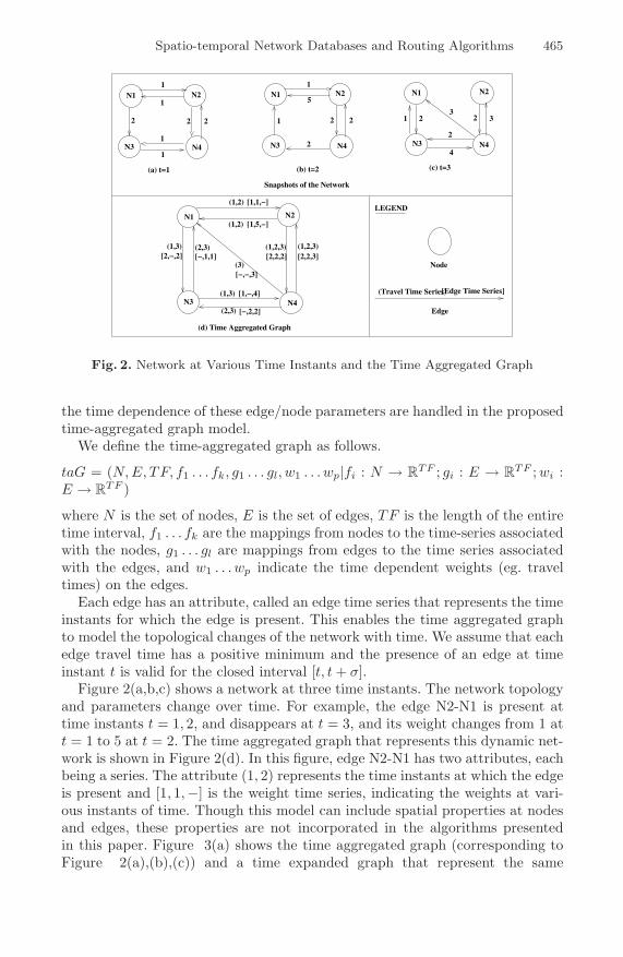
Fig. 2. Network at Various Time Instants and the Time Aggregated Graph

the time dependence of these edge/node parameters are handled in the proposedtime-aggregated graph model.

We define the time-aggregated graph as follows.

taG = (N, E, TF, f1 . . . fk, g1 . . . gl, w1 . . . wp|fi : N → RTF ; gi : E → R

TF ; wi :E → R

TF )

where N is the set of nodes, E is the set of edges, TF is the length of the entiretime interval, f1 . . . fk are the mappings from nodes to the time-series associatedwith the nodes, g1 . . . gl are mappings from edges to the time series associatedwith the edges, and w1 . . . wp indicate the time dependent weights (eg. traveltimes) on the edges.

Each edge has an attribute, called an edge time series that represents the timeinstants for which the edge is present. This enables the time aggregated graphto model the topological changes of the network with time. We assume that eachedge travel time has a positive minimum and the presence of an edge at timeinstant t is valid for the closed interval [t, t + σ].

Figure 2(a,b,c) shows a network at three time instants. The network topologyand parameters change over time. For example, the edge N2-N1 is present attime instants t = 1, 2, and disappears at t = 3, and its weight changes from 1 att = 1 to 5 at t = 2. The time aggregated graph that represents this dynamic net-work is shown in Figure 2(d). In this figure, edge N2-N1 has two attributes, eachbeing a series. The attribute (1, 2) represents the time instants at which the edgeis present and [1, 1, −] is the weight time series, indicating the weights at vari-ous instants of time. Though this model can include spatial properties at nodesand edges, these properties are not incorporated in the algorithms presentedin this paper. Figure 3(a) shows the time aggregated graph (corresponding toFigure 2(a),(b),(c)) and a time expanded graph that represent the same


(a) Time−aggregated Graph

N3N3

N1 N1 N1 N1

N4 N4 N4 N4

t=1 t=2 t=3 t=4 t=5 t=6 t=7

N3

(b) Time Expanded Graph

N1

N2

N3

N4 N4

N3

N2

N1 N1

N2N2 N2 N2 N2

N3

N4

N3

[2,−,2] [−,1,1]

[−,−,3]

[2,2,3]

(1,2)

(1,2)

(1,3) (2,3)[2,2,2](1,2,3) (1,2,3)

(3)

[1,−,4](1,3)

[−,2,2](2,3)

[1,5,−]N1 N2

N3 N4

[1,1,−]

Fig. 3. Time-aggregated Graph vs. Time Expanded Graph

scenario. Edge weights in a time expanded graph are not explicitly shown asedge attributes; instead they are represented by edges that connect the copiesof the nodes at various time instants. For example, the weight 1 of edge N2-N1at t = 1 is represented by connecting the copy of node N2 at t = 1 to the copyof node N1 at time t = 2. The time expansion for the example network needs togo through 7 steps since the latest edge traversal in the network ends at t = 7.The traversal of the edge N3-N4 that starts at t = 3 ends at t = 7, the traveltime of the edge being 4 units. The number of nodes is larger by a factor of T ,where T is the number of time instants and the number of edges is also larger innumber compared to the time-aggregated graph. If the value of T is very large ina spatial network, it would result in enormously large time expanded networksand consequently slow computations.

Comparison of Storage Costs with Time Expanded Networks: Accord-ing to the analysis in [20], the memory requirement for a time expanded networkis O(nT )+O(n+mT ), where n is the number of nodes, m is the number of edgesin the original graph, and T is the length of the travel time series. The memoryrequirement for the time-aggregated graphs would be O(n + m)T , assuming anadjacency list representation of the graph. Each edge has a travel time seriesassociated with it, instead of a scalar cost as in the case of a static graph.

This comparison shows that the memory usage of time-aggregated graphs isless than that of time expanded graphs by a factor of O(nT ).

2.2 Shortest Path Computation for Time Aggregated Graphs(SP-TAG Algorithm)

In time dependent networks, the shortest path and its traversal time are depen-dent on the start time at the source node. Here we give an outline of the algorithmthat computes the shortest path for a given start time in a time-dependent net-work. The algorithm uses the time aggregated graph to represent the network.The application of a greedy strategy in the shortest path computation (whichis a popular choice in most optimization problems) in a time-aggregated graph


N3

N4 N5

1

2 21

1

[1,2,5,8]

[1,2,3,4]

[1,2,3,4]

[1,2,3,4]

[1,2,3,4]

Edge

Node

LegendN2

Travel Time

Edge Time Series

N1

Fig. 4. Optimal Sub-structure of Shortest Paths

faces a challenge. Not all shortest paths display the optimal sub-structure, asillustrated by Figure 4. For the sake of simplicity, the travel times are constantin this example. It can be seen that a shortest path (N1-N3-N4-N5) from N1 toN5 for the start time t = 1, which takes 5 time units, does not display optimalsubstructure. The path from N1 to N4 following the above path is not optimal(shortest path being N1-N2-N4). Although such paths that do not display opti-mal sub-structure could exist, it can be proved that there is at least one optimalpath which satisfies the optimal sub-structure property [8]. This result enablesus to use a greedy approach to compute the shortest path. The algorithm, calledthe SP-TAG algorithm, uses greedy strategy to find the shortest path for a fixedstart time. Every node has a cost associated with it which represents the traveltime to reach the node from the source node. The algorithm picks the node withthe least cost and updates the costs of its adjacent nodes. While finding theadjacent nodes, each edge is selected at its earliest available time instant (min toperation in the algorithm description). A trace of the algorithm is given inTable 1. The table entries are the costs associated with each node (representingthe arrival times at the node) at each iteration. The node marked as “closed”is the node with the minimum cost selected for expansion. The travel times areassumed to follow the FIFO property.

Lemma 1: The SP-TAG algorithm is correct.

Proof: As Figure 4 illustrates, the shortest path fails to have optimal struc-ture due to a potential wait at the intermediate node (u), after reaching thisnode traversing the optimal path from s to u. Consider the optimal path froms to u. Append this path to the path u − d (allowing a wait at the intermedi-ate node u) from the optimal path. This would be still the shortest path froms to d. Otherwise, it would contradict the optimality of the original shortest path.

Lemma 2: The time complexity of the SP-TAG algorithm is O(m(log T +logn))where T is the number of time instants, n is the number of nodes and m is thenumber of edges in the time aggregated graph.


Algorithm 1. Shortest Path (SP-TAG) AlgorithmInput:

1) G(N, E): a graph G with a set of nodes N and a set of edges E;Each node n ∈ N has a property:

Node Presence Time Series : series of positive integers;Each edge e ∈ E has two properties:

Edge Presence Time Series,Travel time series : series of positive integers;

σu,v(t) - travel time of edge uv at time t.2) s: Source node, s ⊆ N; 3) d: Destination node, d ⊆ N;4) tstart: Start Time;

Output: Shortest Route from s to d for tstart

Method:c[s] = tstart; ∀v �= s, c[v] = ∞;// c[u] is the cost at the node u.Insert s in priority queue Q.while Q is not empty do {

u = extract min(Q);for each node v adjacent to u do {

t = min t((u, v), c[u]);if t + σu,v(t) < c[v] {

c[v] = t + σu,v(t); parent[v] = u;if v is not in Q, insert v in Q;

}update Q;

}}

}Output the route from s to d.

Proof: The cost model analysis assumes an adjacency list representation of thegraph with two significant modifications. The edge time series is stored in thesorted order. Attached to every adjacent node in the linked list are the edge timeseries and the travel time series.

For every node extracted from the priority queue Q, there is one edge timeseries look up and a priority queue update for each of its adjacent nodes. Thetime complexity of this step is O(log T + log n). The asymptotic complexity ofthe algorithm would be

O(Σv∈N [degree(v).(log T + log n]) = O(m(log T + log n)).

The time complexity of the SP-TAG shortest path algorithm based on a timeexpanded network is O(nT log T + mT ) [3]. It can be seen that the algorithmbased on a time-aggregated graph is faster if log n < T log T .


Table 1. Trace of the SP-TAG Algorithm for the Network shown in Figure 4

Iteration N1 N2 N3 N4 N5

1 1 (closed) ∞ ∞ ∞ ∞2 1 2 (closed) 3 ∞ ∞3 1 2 3 (closed) 3 ∞4 1 2 3 3 (closed) 65 1 2 3 3 6 (closed)

3 Case Study: Best Start Time Shortest Paths

The time dependency of network parameters affects the connectivity and theshortest paths between nodes in a spatial network. As illustrated in Figure 5,the travel time from node N1 to node N3 changes with the start time. If thetravel starts at t = 1, the commute time would be 6 units. A journey that startsat t = 1 reaches N2 at t = 2 and waits at N2 until edge N2-N3 becomes availableat t = 5, thus taking a total travel time of 6 units to reach node N3. Thetravel on the same route would take 4 units if the start time is moved to t = 4.This shows that the shortest paths in a time-dependent network vary with time,which adds an interesting dimension to shortest path computation. A path thattakes the smallest travel time for a source-destination traversal over the entiretime horizon (called ’Best Start Time shortest Path’) can be computed. This issignificant since it suggests that it is possible to reduce the travel time for thesame source-destination pair if the travel starts at the “right” time instant.

The formulation of algorithms to compute the paths that take the least com-mute time becomes non-trivial since most of the techniques that are used instatic networks might not be applicable in dynamic scenarios. Since the networkchanges in its parameter values and the topology, meeting the requirements ofefficiency and correctness can pose challenges. The potential waits at intermedi-ate nodes can increase the total journey time even if an initial part of the pathturns out to be optimal. Figure 5 shows a spatial network that changes withtime. The figure shows the snapshots of the network at various instants of time,and the edges are marked with the travel times. It is significant to note that theprefix journeys of the best start time shortest path journey are not always opti-mal since some optimal prefix journeys can lead to longer waits at intermediatenodes. The best start time for a journey from node N1 to Node N3 is t = 4,which takes 4 time units. The optimal path from N1 to N3 that starts at t = 4

N1 N3N2

N1 N3N2 N1 N3N2

N1 N3 N1 N3

N1 N3

1 2 2

2 2 2

2

2 2

N2 N2

N2

t=1 t=3

t=4 t=5 t=6

t=2

Node

Edge

Legend

Travel time

Fig. 5. Network at various instants


is not optimal for the intermediate node N2. The best start time for a path fromN1 to N2 is t = 1, which proves to be sub-optimal for a journey from N1 to N3.The lack of an optimal substructure in the best start time shortest paths rulesout the possibility of using a greedy strategy in the algorithm design.

We propose an algorithm that computes the best start time based on a node-cost time series. The proposed algorithm uses the time aggregated network modelto represent a time dependent spatial network.

3.1 BEst Start Time Shortest Path (BEST) Algorithm

While computing the best start time, each node needs to keep track of the traveltimes to the destination for every start time instant. The proposed algorithmattributes each node with a time series, with ith entry representing the current,least travel time to the destination node for the start time ti. Due to the lackof optimality of prefix paths and lack of ordering of nodes based on the costs(ie. travel times), nodes cannot be selected and “closed” based on a minimumscalar cost. The algorithm uses an iterative, label correcting approach [1] andeach entry in a node time series is modified according to the following condition.

Cu[t] = minimum{Cu[t], σuv(t) + Cv[t + σuv(t)]} where, uv ∈ E (1)

Cu[t] - Travel time from u ∈ N to the destination for the start time t.σuv(t) - Travel time of the edge uv at time t.

The algorithm maintains a list of all nodes that change its cost according to thecondition and terminates when there is no further improvement indicated by anempty list. Though the list can be implemented using several data structures,studies on static networks [25,1] have shown that the Two Q implementation [16]of label correcting algorithms performs the best on road networks.

The search starts at the destination node and proceeds to update the remain-ing nodes, finally finding the best start time shortest paths from all nodes to thedestination. Figure 6 illustrates the trace of the algorithm on a small network.In this example, the destination node is the node N4. The node cost series C4is initalized to [0, 0, 0, 0, 0] and the cost series Ci, i = 1, 2, 3 are initialized to[∞, ∞, ∞, ∞, ∞]. The nodes that have N4 in their adjacency lists (that is, allnodes Ni such that NiN4 ∈ E), N2 and N3 are relaxed according to condition(1). These nodes are added to the queue since there is a change in their costseries. The steps continue until the queue is empty, indicating that there is nofurther cost improvement at any of the nodes. At every iteration, the node thatcontributes to a cost improvement is stored in a descendant array to facilitatethe trace of the shortest paths when the algorithm terminates. At the termina-tion, the cost time series has the travel times for every start time t = 1, 2 · · ·T .For example, the cost time series of node N1 shows that the travel times fromN1 to N4 for start times t = 1 is 4 time units, while the best start time at thisnode is t = 4, which results in a travel time of 2 time units and a best start timeshortest path N1-N2-N4. N1-N2 takes 1 time unit at t = 4, reaches N2 at t = 5and continues on N2-N4 at t = 5, reaching N4 at t = 6, taking a total traveltime of 2 time units. A more detailed trace is shown in Table 2.


Algorithm 2. BEST AlgorithmInput:

G(N, E): a graph G with a set of nodes N and a set of edges E;Each node n ∈ N has a property:

Node Presence Time Series : series of positive integers;Each edge e ∈ E has two properties:

Edge Presence Time Series,Travel time series : series of positive integers;

σu,v(t) - travel time of edge uv at time t.Output:

Best Start Time shortest route from s to d;Intialize;While Queue not Empty

v = Dequeue();For every node u such that uv ∈ E

For every entry in the cost series Cu of uif Cu(t) > σuv(t) + Cv(t + σuv(t))

Update Cu(t);Enqueue(u);Update the descendant array of u.

Find the minimum entry in the node time series.Return the BestStartTime and the ShortestRoute;

Table 2. Trace of the BEST Algorithm for the Network shown in Figure 6

Iteration N1 N2 N3 N4 Queue

1 ∞ · · · ∞ ∞· · · ∞ ∞ · · · ∞ [0, 0, 0, 0, 0] N12 ∞ · · · ∞ [1, 1, 2, 2, 1] [4, 4, 2, 4, 3] [0, 0, 0, 0, 0] N2, N33 ∞ · · · ∞ [1, 1, 2, 2, 1] [2, 3, 2, 4, 3] [0, 0, 0, 0, 0] N34 [4, 3, 3, 2, 3] [1, 1, 2, 2, 1] [2, 3, 2, 4, 3] [0, 0, 0, 0, 0] N15 [4, 3, 3, 2, 3] [1, 1, 2, 2, 1] [2, 3, 2, 4, 3] [0, 0, 0, 0, 0] –

Lemma 3: The algorithm terminates and computes the best start time pathsfrom every node to the destination.

Proof: The algorithm terminates because there is a positive minimum for thetravel time over every path, for every pair of nodes in the network since theedge weights (travel times) are positive and each such path has a finite numberof edges. The updates on the costs according to condition(1) will generate theoptimal travel times from a node to the destination at the termination of thealgorithm. This can be proved by induction on the number of edges on the path.The base condition would be for paths with two edges, say from any node uto the destination node d. Every path with two edges from u to d will transitto some node v and then traverse the edge to d which takes the least time. Ifwe assume the inductive hypotheses is true for every path with k edges, the


4 4 4 4 41 1 2 2 1[ ]

2 2 4 4 42 3 2 4 3[ ]

2 2 2 2 25 5 3 2 3[ ]

3 3 2 2 24 3 3 2 3[ ]

0 0 0 0 0[ ]− − − −−

0 0 0 0 0[ ]1

− −−

0 0 0 0 0[ ]− − − −−

(Result)Best Start Time: 4Route: 1 − 2 − 4

1

3

4 4 4 4 41 1 2 2 1[ ]

2 2 4 4 42 3 2 4 3[ ]

−

4

(Input Network)

(Step 1)

(Step 2)

(Step 3)

(Step 4)

(Legend)

Parent Pointer List[ ]Distance List from Destination

4

4

2

3

Expansion Node

Best Start Time

− − −−

2

#

−

ooo oooo[ ]− − − − −

2

1 4

3

o2

1 4

3 oooooo oooo[ ]− − − − −

oo

(4,4,1,1,2)

]− − − − −

oooooo oooo[ ]− − − − −

0 0 0 0 0[ ]−[

(1,1,2,2,1)

(1,1,2,2,3) (4,4,2,4,3)

(1,1,1,3,2)

2

1

3

4 4 4 4 41 1 2 2 1[ ]

oooooooo oo

][ 4 4 2 4 34 4 4 4 4

Fig. 6. Trace of the BEST Algorithm

minimality must hold for a path from u with (k + 1) edges since we can reachnode u that with a minimal k−edge path and append uv with travel time σuv(t).

Lemma 4: The computational complexity of the BEST algorithm is O(n2mT ),where n is the number of nodes, m is the number of edges and T is the lengthof the time series.

Proof: The worst case computational complexity of the label correcting algo-rithm based on Two-Q data structure is O(n2m) when the node costs and edgeweights are scalar quantities [1]. In the BEST algorithm, the relaxation stepoperates on a time series (node cost and edge weight) of length T . Hence thecomputational complexity of the algorithm is O(n2mT ).

4 Experimental Analysis

In this section, the experimental analysis of the BEST algorithm and the SP-TAG algorithm are provided. The purpose of the performance evaluation of thealgorithm is to compare the run-times with algorithms based on a time-expandedgraph.

Experiment Design. Figure 7 illustrates the experiment design to comparethe performance of the proposed algorithm and the algorithm based on a timeexpanded network. Time expanded graphs make copies of the original network


AnalysisAdd TimeDimension

GenerateTime Series

Read Data without Time Series

Best Start TimeShortest Path Algorithm

Algorithm based onTime Expanded Graph

Length of Time Series

Fig. 7. Experiment Design

for every time instant under consideration. The model used for the proposedalgorithm is time-aggregated graphs. In our experiments the following were se-lected as the independent parameters: 1) network size represented by number ofnodes; and 2) the length of the time interval in terms of number of time instants.The data sets have two main components: (1) the network data that consists ofthe graph structure and (2) the travel time series. The networks chosen are roadmaps from the Minneapolis downtown area with radii of .5 mile, 1 mile, 2 milesand 3miles. This is appended with travel time series of various lengths. Thetravel time series were synthetically generated. This data was fed to both a timeexpanded graph generator, which generates the expanded graph encoding thetravel time information. An algorithm for for computing the shortest path for agiven start time was run on this graph. The SP-TAG algorithm was run on thesame dataset and the results were compared. The time expanded graph was thenused to find the start time that results in the least travel time and the resultswere compared to the results from the BEST algorithm.

The experiments were conducted on a SUN Solaris workstation with 1.77GHzCPU, 1GB RAM and UNIX operating system. Each experimental result reportedin the following sections is the average over 5 experiment runs with networksgenerated using the same input parameters, but with different destination nodes.

4.1 Experimental Results and Anlaysis

We wanted to answer three questions: (1) How does the network size (numberof nodes, number of edges) affect the performance of the algorithms? (2) Howdoes the length of the time series affect the performance of the algorithms? (3)How do the the two representations, time expanded graph and time aggregatedgraph, compare with respect to algorithm performance?

Experiment 1: How does the network size affect the performance of the algo-rithms?The purpose of the first experiment was to evaluate how the network size interms of the number of nodes affects the performance of the algorithms. Wefixed the length of the travel time series, and varied the network size to observe


Table 3. Description of Datasets

Dataset Radius No: of Nodes No: of Edges

1 0.5 mile 111 2872 1 mile 277 6743 2 miles 562 14434 3 miles 786 2106

111

Ru

n t

ime

in s

econ

ds

(log

sca

le)

Time Expanded Graph

277 562 786

1000

100

10

1

0.1

Number of Nodes

SP−TAG Algorithm

Fig. 8. SP-TAG Algorithm: Run-time With Respect to Network Size

111

Ru

n t

ime

in s

econ

ds

(log

sca

le)

Time Expanded Graph

BEST Algorithm

277 562 786

Number of Nodes

1

10

100

1000

10000

Fig. 9. BEST Algorithm: Run-timeWith Respect to Network Size

the run times of both the fixed start time(SP-TAG) and best start time(BEST)algorithms and time-expanded graph based algorithms.

The experiment was done with four datasets that represent the road mapsfrom the Minneapolis downtown area of .5 mile, 1 mile, 2 mile and 3mile radius.The length of the time series was fixed at 240. The number of nodes and edges inthese datasets are provided in Table 3. Figure 8 shows the run-time of the fixedstart time algorithm based on the time aggregated graph and the performance ofthe algorithm based on the time expanded graph. The SP-TAG algorithm runsfaster than the time-expanded graph based algorithm in all cases; further, itsrun-time seens to increase at a slower rate. Figure 9 shows the performance ofthe BEST algorithm and that of the time expanded graph algorithm. The runtime of the BEST algorithm is much lower than that of the time expanded graphalgorithm.

Experiment 2: How does the length of the time series affect the performnace ofthe algorithms?In the second experiment, we evaluated how the number of time instants affectsthe performance of the algorithms. We fixed the network size, and varied thelength of the time series to observe the run-time. The number of time instantswas varied from 120 to 480 and the network size parameters were fixed at 562nodes and 1443 edges. As seen in Figure 10, the SP-TAG algorithm performs


1

10

100

1000

10000

120 240 360 480


Ru

n t

ime

in s

econ

ds

(log

sca

le)

Time Expanded Graph

SP−TAG Algorithm

Fig. 10. SP-TAG Algorithm: Run-timeWith Respect to Length of Time series

1

10

100

1000

10000

120 240 360 480


Ru

n t

ime

in s

econ

ds

(log

sca

le)

Time Expanded Graph

BEST Algorithm

Fig. 11. BEST Algorithm: Run-time WithRespect to Length of Time series

better. Figure 11 shows the performance of the BEST algorithm and that of thetime expanded graph algorithm. As the length of the time series increases, thenumber of copies of the entire network required in the case of the time expandedgraph increases, resulting in a considerable increase in the size of the entirenetwork, leading to almost exponential increases in run time.

3: How do the the two representations, time expanded graph and time aggregatedgraph, compare with respect to algorithm performance?Based on the results of Experiments (1) and (2), it can be seen that algorithmsbased on the time aggregated graph perform better than those based on the timeexpanded graph.

5 Conclusions and Future Work

Spatio-temporal networks form a key part of critical applications such as emer-gency planning and there is a great need for database support in this area. Thepaper describes a model to represent a spatio-temporal network and proposes twoalgorithms for shortest path computations. The formulation of these algorithmsis based on a model for spatio-temporal networks called time-aggregated graphs.In addition to the algorithm that computes the shortest path for a given starttime, we also addressed the time-dependence of shortest paths in networks byformulating an algorithm that computes shortest paths which result in the leasttravel time over the entire time period. We also present an experimental analysisof the best start time (BEST) algorithm and the fixed start time algorithm (SP-TAG) (which was proposed in [8]). Experiments show that the algorithms basedon time aggregated graphs significantly reduce the computational cost comparedto similar algorithms based on time expanded networks.

We plan to evaluate the performance of the algorithms using real-trafficdatasets shortly. We recently acquired a dataset for interstate highway I-66.


This data contains time-stamped occupancy, speed and volume collected from anumber of stations on I-66 on November 6, 2006 using the Advanced InteractiveTraffic Visualization System [23]. We anticipate that this evaluation will givenew insights into the average case run time of the algorithms, which we expectto be significantly better than the worst case complexity, especially in the caseof the BEST algorithm based on a label correcting approach. We are also plan-ning to extend our experiments with Google traffic data and traffic archive datacollected by the Traffic Management Center at the University of Minnesota.

The time aggregated graphs can accomodate the time-varying capacities ofthe road networks. The proposed algorithms need to be extended to give opti-mal solutions subject to the constraints of time-varying capacities. This wouldextend the use of the algorithms to domains such as evacuation planning inemergency management, where capacity constraints in the network pose signif-icant challenges. We plan to include spatial attributes at nodes and edges andincorporate necessary changes in the algorithms. We plan to incorporate the al-gorithms as building blocks that find the shortest paths in the CCRP evacuationplanner [13]. We will also explore other graph problems in the context of timeaggregated graphs.

Acknowledgments

We are particularly grateful to the members of the Spatial Database ResearchGroup at the University of Minnesota for their helpful comments and valuablesuggestions. We would also like to express our thanks to Kim Koffolt for improv-ing the readability of this paper.

This work was supported by the NSF SEI grant and Minnesota Departmentof Transportation. The content does not necessarily reflect the position or thepolicy of the government and no official endorsement should be inferred.

References

1. Cherkassky, B.V., Goldberg, A.V., Radzik, T.: Shortest Paths Algorithms: Theoryand Experimental Evaluation . Mathematical Programming 73, 129–174 (1996)

2. Cormen, T.H., Leiserson, C.E., Rivest, R.L., Stein, C.: Introduction to Algorithms(Chapter 26, Flow Networks). MIT Press, Cambridge, MA, USA (2002)

3. Dean, B.C.: Algorithms for minimum-cost paths in time-dependent networks. net-works 44(1), 41–46 (2004)

4. Ding, Z., Guting, R.H.: Modeling temporally variable transportation networks.Proc. 16th Intl. Conf. on Database Systems for Advanced Applications , 154–168(2004)

5. Erwig, M.: Graphs in Spatial Databases. PhD thesis, Fern Universitat Hagen (1994)6. Erwig, M., Guting, R.H.: Explicit graphs in a functional model for spatial

databases. IEEE Transactions on Knowledge and Data Engineering 6(5), 787–804(1994)

7. ESRI. ArcGIS Network Analyst (2006),http://www.esri.com/software/arcgis/extensions/

http://www.esri.com/software/arcgis/extensions/


8. George, B., Shekhar, S.: Time-aggregated Graphs for Modeling Spatio-TemporalNetworks - An Extended Abst ract . Proceedings of Workshops at InternationalConference on Conceptual Modeling (2006)

9. Hamre, T.: Development of Semantic Spatio-temporal Data Models for Integrationof Remote Sensing and in situ Data in Marine Information System. PhD thesis,University of Bergen, Norway (1995)

10. Kaufman, D.E., Smith, R.L.: Fastest paths in time-dependent networks for intelli-gent vehicle highway systems applications. IVHS Journal 1(1), 1–11 (1993)

11. Kohler, E., Langtau, K., Skutella, M.: Time-expanded graphs for flow-dependenttransit times. In: Proc. 10th Annual European Symposium on Algorithms, pp.599–611 (2002)

12. Sellis, T., Koubarakis, M., Frank, A., Grumbach, S., Guting, R.H., Jensen,C., Lorentzos, N.A., Manolopoulos, Y., Nardelli, E., Pernici, B., Theodoulidis,B., Tryfona, N., Schek, H.-J., Scholl, M.O.: Spatio-Temporal Databases: TheCHOROCHRONOS Approach. In: Sellis, T., Koubarakis, M., Frank, A., Grum-bach, S., Guting, R.H., Jensen, C., Lorentzos, N.A., Manolopoulos, Y., Nardelli,E., Pernici, B., Theodoulidis, B., Tryfona, N., Schek, H.-J., Scholl, M.O. (eds.)Spatio-Temporal Databases. LNCS, vol. 2520, Springer, Heidelberg (2003)

13. Lu, Q., George, B., Shekhar, S.: Capacity Constrained Routing Algorithms forEvacuation Planning: A Summary of Resu lts. In: Bauzer Medeiros, C., Egenhofer,M.J., Bertino, E. (eds.) SSTD 2005. LNCS, vol. 3633, Springer, Heidelberg (2005)

14. Oracle. Oracle Spatial 10g, An Oracle White Paper. August (2005),http://www.oracle.com/technology/products/spatial/

15. Orda, A., Rom, R.: Minimum weight paths in time-dependent networks. net-works 21, 295–319 (1991)

16. Pallottino, S.: Shortest-Path Methods: Complexity, Interrelations and New Propo-sitions. Networks 14, 257–267 (1984)

17. Pallottino, S., Scuttella, M.G.: Shortest path algorithms in tranportation models:Classical and innovative aspects. Equilibrium and Advanced transportation Mod-elling , 245–281 (1998)

18. Rasinmaki, J.: Modelling spatio-temporal environmental data. In: 5th AGILE Con-ference on Geographic Information Science, Palma, Balearic Islands, Spain (April2002)

19. Shekhar, S., Chawla, S.: Spatial Databases: Tour. Prentice-Hall, Englewood Cliffs(2003)

20. Sawitzki, D.: Implicit Maximization of Flows over Time. Technical report, Univer-sity of Dortmund (2004)

21. Dreyfus, S.E.: An appraisal of some shortest path algorithms. Operations Re-search 17, 395–412 (1969)

22. Shekhar, S., Liu, D.: CCAM: A Connectivity-Clustered Access Method for Net-works and Networks Computations. IEEE Transactions on Knowledge and DataEngineering, 9 (January 1997)

23. Spatial Data Management Lab, Virginia Polytechnic Institute and State Uni-versity. AITVS: Advanced Interactive Traffic Visualization System (2007),http://spatial.nvc.cs.vt.edu/traffic zhh/

24. Stephens, S., Rung, J., Lopez, X.: Graph data representation in oracle databese10g: Case studies in life sciences. IEEE Data Engineering Bulletin 27(4), 61–66(2004)

25. Zhan, F.B., Noon, C.E.: Shortest Paths Algorithms: An Evaluation Using RealRoad Networks. Transportation Science 32, 65–73 (1998)

http://www.oracle.com/technology/products/spatial/

http://spatial.nvc.cs.vt.edu/traffic_zhh/

spatio-temporal network databases and routing algorithms ... · spatio-temporal network databases...

Documents