spatially distributed sampling and - … data exchange network requires signi cant e orts (due to...

SPATIALLY DISTRIBUTED SAMPLING ANDRECONSTRUCTION

CHENG CHENG, YINGCHUN JIANG AND QIYU SUN

Abstract. A spatially distributed system contains a large amount of agentswith limited sensing, data processing, and communication capabilities. Recenttechnological advances have opened up possibilities to deploy spatially distributedsystems for signal sampling and reconstruction. In this paper, we introduce agraph structure for a distributed sampling and reconstruction system by couplingagents in a spatially distributed system with innovative positions of signals. A fun-damental problem in sampling theory is the robustness of signal reconstruction inthe presence of sampling noises. For a distributed sampling and reconstructionsystem, the robustness could be reduced to the stability of its sensing matrix. Ina traditional centralized sampling and reconstruction system, the stability of thesensing matrix could be verified by its central processor, but the above procedureis infeasible in a distributed sampling and reconstruction system as it is decen-tralized. In this paper, we split a distributed sampling and reconstruction systeminto a family of overlapping smaller subsystems, and we show that the stability ofthe sensing matrix holds if and only if its quasi-restrictions to those subsystemshave uniform stability. This new stability criterion could be pivotal for the designof a robust distributed sampling and reconstruction system against supplement,replacement and impairment of agents, as we only need to check the uniformstability of affected subsystems. In this paper, we also propose an exponentiallyconvergent distributed algorithm for signal reconstruction, that provides a subop-timal approximation to the original signal in the presence of bounded samplingnoises.

1. Introduction

Spatially distributed systems (SDS) have been widely used in (underwater) mul-tivehicle and multirobot networks, wireless sensor networks, smart grids, etc ([2,19, 23, 74, 75]). Comparing with traditional centralized systems that have a pow-erful central processor and reliable communication between agents and the centralprocessor, an SDS could give unprecedented capabilities especially when creatinga data exchange network requires significant efforts (due to physical barriers suchas interference), or when establishing a centralized processor presents the dauntingchallenge of processing all the information (such as big-data problems). In this pa-per, we consider SDSs for signal sampling and reconstruction, and we describe the

Key words and phrases. Spatially distributed systems, distributed sampling and reconstructionsystems, signals on a graph, distributed algorithms, finite rate of innovation, Beurling dimensions,localized matrices, inverse-closed subalgebras.

This project is partially supported by the National Natural Science Foundation of China (Nos.11201094 and 11161014), Guangxi Natural Science Foundation (2014GXNSFBA118012), and theNational Science Foundation (DMS-1412413).

1

arX

iv:1

511.

0854

1v1

[cs

.IT

] 2

7 N

ov 2

015

2 CHENG CHENG, YINGCHUN JIANG AND QIYU SUN

topology of an SDS by an undirected (in)finite graph

(1.1) G := (G,S),

where a vertex represents an agent and an edge between two vertices means that adirect communication link exists.

In the SDS described above, sampling data of a signal f acquired by the agentλ ∈ G is

(1.2) y(λ) := 〈f, ψλ〉,where ψλ is the impulse response of the agent λ ∈ G ([4, 7, 8, 32, 48, 57, 59, 70,71, 72]). Fundamental signal reconstruction problems are whether and how thesignal f can be recovered from its sampling data y(λ), λ ∈ G. For well-posedness,the signal f of interest is usually assumed to have additional properties, such asband-limitedness, finite rate of innovation, smoothness, and sparse expansion in adictionary ([7, 15, 26, 27, 28, 71, 72]). In this paper, we consider spatial signals withthe following parametric representation,

(1.3) f :=∑i∈V

c(i)ϕi,

where amplitudes c(i), i ∈ V , are bounded, and generators ϕi, i ∈ V , are essentiallysupported in a spatial neighborhood of the innovative position i. The above family ofspatial signals appears in magnetic resonance spectrum, mass spectrometry, globalpositioning system, cellular radio, ultra wide-band communication, electrocardio-gram, and many engineering applications, see [27, 61, 72] and references therein.

In this paper, we associate every innovative position i ∈ V with some anchoragents λ ∈ G, and denote the set of such associations (i, λ) by T . These associationscan be easily understood as agents within certain (spatial) range of every innovativeposition. With the above associations, we describe our distributed sampling andreconstruction system (DSRS) by an undirected (in)finite graph

(1.4) H := (G ∪ V, S ∪ T ∪ T ∗),where T ∗ = {(λ, i) ∈ G× V, (i, λ) ∈ T}, see Figure 1. The above graph descriptionof a DSRS plays a crucial role for us to study signal sampling and reconstruction.

Given a DSRS described by the above graph H, set

(1.5) E := {(i, i′) ∈ V × V, i 6= i′ and (i, λ), (i′, λ) ∈ T for some λ ∈ G}.We then generate a graph structure

(1.6) V := (V,E)

for signals in (1.3), where an edge between two distinct innovative positions in Vmeans that a common anchor agent exists. The above graph structure for signalsis different from the conventional one in most of the literature, where the graph isusually preassigned. The reader may refer to [52, 53, 56] and Remark 3.6.

Define sensing matrix S of our DSRS by

(1.7) S := (〈ϕi, ψλ〉)λ∈G,i∈V .

SPATIALLY DISTRIBUTED SAMPLING AND RECONSTRUCTION 3

Figure 1. The graph H = (G∪V, S ∪T ∪T ∗) in (1.4) to describe aDSRS, where vertices in G and V are plotted in red circles and bluetriangles, and edges in S, T and E are in black solid lines, green solidlines and red dashed lines respectively.

The sensing matrix S is stored by agents in a distributed manner. Due to thestorage limitation, each agent in our SDS stores its corresponding row (and perhapsalso its neighboring rows) in the sensing matrix S, but it does not have the wholematrix available. Agents in our SDS have limited acquisition ability and they couldessentially catch signals not far from their physical locations. So the sensing matrixS has certain polynomial off-diagonal decay, i.e., there exist positive constants Dand α such that

(1.8) |〈ϕi, ψλ〉| ≤ D(1 + ρH(λ, i))−α for all λ ∈ G and i ∈ V,

where ρH is the geodesic distance on the graph H. For most DSRSs in applications,such as multivehicle and multirobot networks and wireless sensor networks, thesignal generated at any innovative position could be detected by its anchor agentsand some of their neighboring agents, but not by agents in the SDS far away. Thusthe sensing matrix S may have finite bandwidth s ≥ 0,

(1.9) 〈ϕi, ψλ〉 = 0 if ρH(λ, i) > s.

The above global requirements (1.8) and (1.9) could be fulfilled in a distributedmanner.

The sensing matrix S characterizes the sampling procedure (1.2) of signals withthe parametric representation (1.3). Applying the sensing matrix S, we obtain thesample vector y = (〈f, ψλ〉)λ∈G of the signal f from its amplitude vector c :=(c(i))i∈V ,

(1.10) y = Sc.

Under the assumptions (1.8) and (1.9), it is shown in Proposition 4.1 that a signal fwith bounded amplitude vector c generates a bounded sample vector y. Thus there


exists a positive constant C such that

‖y‖∞ ≤ C‖c‖∞ for all c ∈ `∞,where for 1 ≤ p ≤ ∞, `p is the space of all p-summable sequences with norm ‖ · ‖p.

A fundamental problem in sampling theory is the robustness of signal reconstruc-tion in the presence of sampling noises ([10, 32, 46, 47, 48, 51, 57]). In this paper,we consider the scenario that the sampling data y = Sc is corrupted by boundeddeterministic/random noise ηηη = (η(λ))λ∈G,

(1.11) z = Sc + ηηη

([66, 73]). For the robustness of our DSRS, one desires that the signal reconstructedby some (non)linear algorithm ∆ is a suboptimal approximation to the original sig-nal, in the sense that the differences between their corresponding amplitude vectors∆(z) and c are bounded by a multiple of noise level δ = ‖ηηη‖∞, i.e.,

(1.12) ‖∆(z)− c‖∞ ≤ Cδ

for some absolute constant C ([1, 7, 17]).Given the noisy sampling vector z in (1.11), solve the following nonlinear problem

of maximal sampling error ([13, 14]),

(1.13) ∆∞(z) := argmind∈`∞

‖Sd− z‖∞.

Observe from (1.11) and (1.13) that

‖S∆∞(z)− Sc‖∞ ≤ ‖S∆∞(z)− z‖∞ + ‖ηηη‖∞ ≤ ‖Sc− z‖∞ + ‖ηηη‖∞ ≤ 2‖ηηη‖∞.Thus the solution of the `∞-minimization problem (1.13) gives a suboptimal ap-proximation to the true amplitude vector c if the sensing matrix S of the DSRS has`∞-stability ([7, 67, 71]).

Definition 1.1. For 1 ≤ p ≤ ∞, a matrix A is said to have `p-stability if thereexist positive constants A and B such that

(1.14) A‖c‖p ≤ ‖Ac‖p ≤ B‖c‖p for all c ∈ `p.We call the minimal constant B and the maximal constant A for (1.14) to hold theupper and lower `p-stability bounds respectively.

The `∞-stability of a matrix can not be verified in a distributed manner, up toour knowledge. We circumvent such a verification problem by showing in Theorem5.2 that a matrix with some polynomial off-diagonal decay has `∞-stability if it has`2-stability.

Next we consider the problem how to verify `2-stability of the sensing matrix S ofour DSRS in a distributed manner. It is well known that a finite-dimensional matrixS has `2-stability if and only if STS is strictly positive, and its upper and lowerstability bounds are the same as square roots of largest and smallest eigenvalues ofSTS. The above procedure to establish `2-stability for the sensing matrix of ourDSRS is not feasible, because the whole sensing matrix S is not available for anyagent in the DSRS and there is no centralized processor to evaluate eigenvalues ofSTS of large size. In Theorems 6.1 and 6.2, we introduce a method to split the


DSRS into a family of overlapping subsystems of small size, and we show that thesensing matrix S with polynomial off-diagonal decay has `2-stability if and only ifits quasi-restrictions to those subsystems have uniform `2-stability. The new localcriterion in Theorems 6.1 and 6.2 provides a reliable tool for the verification of the`2-stability in a distributed manner. Also it is pivotal for the design of a robustDSRS against supplement, replacement and impairment of agents, as it suffices toverify the uniform stability of affected subsystems.

Then we consider signal reconstructions in a distributed manner, under the as-sumption that the sensing matrix S of our DSRS has `2-stability. For centralizedsignal reconstruction systems, there are many robust algorithms, such as the framealgorithm and the approximation-projection algorithm, to approximate signals fromtheir (non)linear noisy sampling data ([5, 17, 20, 31, 34, 48, 59, 66]). In this paper,we develop a distributed algorithm to find the suboptimal approximation

(1.15) ∆2(z) := (STS)−1STz

to the original signal f in (1.3). For the case that our DSRS has finitely many agents(which is the case in most of practical applications), the suboptimal approximation∆2(z) in (1.15) is the unique least squares solution,

(1.16) ∆2(z) = argmind∈`2

‖Sd− z‖22 = argmin

d∈`2

∑λ∈G

fλ(d, z),

where d = (d(i))i∈V , z = (z(λ))λ∈G, and

(1.17) fλ(d, z) =∣∣∣∑i∈V

〈ϕi, ψλ〉d(i)− z(λ)∣∣∣2, λ ∈ G.

As our SDS has strict constraints in its data processing power and communica-tion bandwidth, we need develop distributed algorithms to solve the optimizationproblem

(1.18) min∑λ∈G

fλ(d, z).

For the case that G = V and the sensing matrix S is strictly diagonally dominant,the Jacobi iterative method,

d1(λ) = 0dn+1(λ) = (〈ϕλ, ψλ〉)−1

(∑i 6=λ〈ϕi, ψλ〉dn(i)− z(λ)

)= argmint∈Rfλ(dn;t,λ, z), λ ∈ G = V, n ≥ 1,

is a distributed algorithm to solve the minimization problem (1.18), where dn;t,λ

is obtained from dn = (dn(i))i∈V by replacing its λ-component dn(λ) with t. Thereader may refer to [9, 16, 42, 45, 49] and references therein for historical remarks,motivations, applications and recent advances on distributed algorithms, especiallyfor the case that G = V .

In our DSRS, the set G of agents is not necessarily the same as the set V ofinnovative positions, and even for the case that the sets G and V are the same, thesensing matrix S need not be strictly diagonally dominant in general. In this paper,we introduce a distributed algorithm (7.19) and (7.20) to approximate ∆2(z) in


(1.15), when the sensing matrix S has `2-stability and satisfies the requirements (1.7)and (1.8). In the above distributed algorithm for signal reconstruction, each agentin the SDS collects noisy observations of neighboring agents, then interacts with itsneighbors per iteration, and continues the above recursive procedure until arrivingat an accurate approximation to the solution ∆2(z) in (1.15). More importantly, weshow in Theorems 7.1 and 7.2 that the proposed distributed algorithm (7.19) and(7.20) converges exponentially to the solution ∆2(z) in (1.15). The establishment forthe above convergence is virtually based on Wiener’s lemma for localized matrices([37, 38, 40, 58, 60, 65]) and on the observation that our sensing matrices are quasi-diagonal block dominated.

The paper is organized as follows. In Section 2, we make some basic assumptionson the SDS and we introduce its Beurling dimension and sampling density. In Section3, we impose some constraints on the graph H to describe our DSRS and then wedefine dimension and maximal rate of innovation for signals on the graph V . We showin Theorem 3.5 that the dimension for signals is the same as the Beurling dimensionfor the SDS, and the maximal rate of innovation is approximately proportional tothe sampling density of the SDS. In Section 4, we prove in Proposition 4.1 thatsampling a signal with bounded amplitude vector by the procedure (1.2) producesa bounded sampling data vector when the sensing matrix of the SDS has certainpolynomial off-diagonal decay. In Section 5, we establish in Theorem 5.2 that ifa matrix with certain off-diagonal decay has `2-stability then it has `p-stability forall 1 ≤ p ≤ ∞, and also in Theorem 5.4 that the solution ∆2(z) in (1.15) is asuboptimal approximation to the true amplitude vector. In Theorems 6.1 and 6.2 ofSection 6, we introduce a criterion for the `2-stability of a sensing matrix, that couldbe verified in a distributed manner. In Section 7, we propose a distributed algorithmto solve the minimization problem (1.16). In Section 8, we present simulations todemonstrate our proposed algorithm for robust signal reconstruction. In Section 9,we include proofs of all conclusions.

The sampling theory developed in this paper enjoys the advantages of scalabilityof network sizes and data privacy preservation. Some results of this paper wereannounced in [18].

Notation: AT is the transpose of a matrix A; ‖c‖p is the norm on `p; χF is theindex function on a set F ; dxe is the ceiling of x ∈ R; bxc is the floor of x ∈ R; #Fis the cardinality of a set F ; and ‖A‖B2 is the operator norm of a matrix A on `2.

2. Spatially distributed systems

Let G be the graph in (1.1) to describe our SDS. In this paper, we always assumethat G is connected and simple (i.e., undirected, unweighted, no graph loops normultiple edges), which can be interpreted as follows:

• Agents in the SDS can communicate across the entire network, but they havedirect communication links only to adjacent agents.• Direct communication links between agents are bidirectional.• Agents have the same communication specification.


• The communication component is not used for data transmission within anagent.• No multiple direct communication channels between agents exists.

In this section, we recall geodesic distance on the graph G to measure communica-tion cost between agents. Then we consider doubling and polynomial growth prop-erties of the counting measure on the graph G, and we introduce Beurling dimensionand sampling density of the SDS. For a discrete sampling set in the d-dimensionalEuclidean space, the reader may refer to [24, 30] for its Beurling dimension and to[7, 48, 59, 71] for its sampling density. Finally, we introduce a special family ofballs to cover the graph G, which will be used in Section 7 for the consensus of ourproposed distributed algorithm.

2.1. Geodesic distance and communication cost. For a connected simple graphG := (G,S), let ρG(λ, λ) = 0 for λ ∈ G, and ρG(λ, λ

′) be the number of edges in ashortest path connecting two distinct vertices λ, λ′ ∈ G. The above function ρG onG × G is known as geodesic distance on the graph G ([21]). It is nonnegative andsymmetric:

(i) ρG(λ, λ′) ≥ 0 for all λ, λ′ ∈ G;

(ii) ρG(λ, λ′) = ρG(λ

′, λ) for all λ, λ′ ∈ G.

And it satisfies identity of indiscernibles and the triangle inequality:

(iii) ρG(λ, λ′) = 0 if and only if λ = λ′;

(iv) ρG(λ, λ′) ≤ ρG(λ, λ

′′) + ρG(λ′′, λ′) for all λ, λ′, λ′′ ∈ G.

Given two nonadjacent agents λ and λ′ ∈ G, the distance ρG(λ, λ′) can be used

to measure the communication cost between these two agents if the communicationis processed through their shortest path.

2.2. Counting measure, Beurling dimension and sampling density. For aconnected simple graph G := (G,S), denote its counting measure by µG,

µG(F ) := ](F ) for F ⊂ G.

Definition 2.1. The counting measure µG is said to be a doubling measure if thereexists a positive number D0(G) such that

(2.1) µG(BG(λ, 2r)) ≤ D0(G)µG(BG(λ, r)) for all λ ∈ G and r ≥ 0,

where

BG(λ, r) := {λ′ ∈ G, ρG(λ, λ′) ≤ r}

is the closed ball with center λ and radius r.

The doubling property of the counting measure µG can be interpreted as numbersof agents in r-neighborhood and (2r)-neighborhood of any agent are comparable.The doubling constant of µG is the minimal constant D0(G) ≥ 1 for (2.1) to hold([22, 25]). It dominates the maximal vertex degree of the graph G,

(2.2) deg(G) ≤ D0(G),


because

deg(G) = maxλ∈G

#{λ′ ∈ G, (λ, λ′) ∈ S} ≤ maxλ∈G

#(BG(λ, 1))≤ D0(G).

We remark that for a finite graph G, its doubling constant D0(G) could be muchlarger than its maximal vertex degree deg(G). For instance, a tree with one branchfor the first L levels and two branches for the next L levels has 3 as its maximalvertex degree and (2L+1 +L− 1)/(L+ 1) as its doubling constant, see Figure 2 withL = 3.

Figure 2. A tree with large doubling constant but limited maximalvertex degree.

The counting measure on an infinite graph is not necessarily a doubling measure.However, the counting measure on a finite graph is a doubling measure and itsdoubling constant could depend on the local topology and size of the graph, cf. thetree in Figure 2. In this paper, the graph G to describe our SDS is assumed to haveits counting measure with the doubling property (2.1).Assumption 1: The counting measure µG of the graph G is a doubling measure,

(2.3) D0(G) <∞.Therefore the maximal vertex degree of graph G is finite,

deg(G) <∞,which could be understood as that there are limited direct communication channelsfor every agent in the SDS.

Definition 2.2. The counting measure µG is said to have polynomial growth if thereexist positive constants D1(G) and d(G) such that

(2.4) µG(BG(λ, r)) ≤ D1(G)(1 + r)d(G) for all λ ∈ G and r ≥ 0.

For the graph G associated with an SDS, we may consider minimal constantsd(G) and D1(G) in (2.4) as Beurling dimension and sampling density of the SDSrespectively. We remark that

(2.5) d(G) ≥ 1,

becausesupλ∈G

µG(BG(λ, r)) ≥ 1 + r for all 0 ≤ r ≤ diam(G),


where diam(G) := supλ,λ′∈G ρG(λ, λ′) is the diameter of the graph G.

Applying (2.1) repeatedly leads to the following general doubling property:

µG(BG(λ, sr)) ≤ (D0(G))dlog2 seµG(BG(λ, r)) ≤ D0(G)slog2D0(G)µG(BG(λ, r))

for all λ ∈ G, s ≥ 1 and r ≥ 0. Thus

µG(BG(λ, r)) ≤ D0(G)(1+r)log2D0(G)µG

(BG

(λ,

r

1 + r

))= D0(G)(1+r)log2D0(G), r ≥ 0.

This shows that a doubling measure has polynomial growth.

Proposition 2.3. If the counting measure µG on a connected simple graph G is adoubling measure, then it has polynomial growth.

For a connected simple graph G, its maximal vertex degree is finite if the countingmeasure µG has polynomial growth, but the converse is not true. We observe thatif the maximal vertex degree deg(G) is finite, then the counting measure µG hasexponential growth,

(2.6) µG(BG(λ, r)) ≤(deg(G))r+1 − 1

deg(G)− 1for all λ ∈ G and r ≥ 0.

2.3. Spatially distributed subsystems. For a connected simple graph G :=(G,S), take a maximal N -disjoint subset GN ⊂ G, 0 ≤ N ∈ R, such that

(2.7) BG(λ,N)∩ (∪λm∈GN BG(λm, N))6= ∅ for all λ ∈ G,

and

(2.8) BG(λm, N)∩BG(λm′ , N) = ∅ for all λm, λm′ ∈ GN .

For 0 ≤ N < 1, it follows from (2.7) that GN = G. For N ≥ 1, there are manysubsets GN of vertices satisfying (2.7) and (2.8). For instance, we can constructGN = {λm}m≥1 as follows: take a λ1 ∈ G and define λm, m ≥ 2, recursively by

λm = argminλ∈Am

ρG(λ, λ1),

where Am = {λ ∈ G, BG(λ,N) ∩BG(λm′ , N) = ∅, 1 ≤ m′ ≤ m− 1}.For a set GN satisfying (2.7) and (2.8), the family of balls {BG(λm, N ′), λm ∈ GN}

with N ′ ≥ 2N provides a finite covering for G.

Proposition 2.4. Let G := (G,S) be a connected simple graph and µG have thedoubling property (2.3) with constant D0(G). If GN satisfies (2.7) and (2.8), then(2.9)

1 ≤ infλ∈G

Σλm∈GNχBG(λm,N ′)(λ) ≤ supλ∈G

Σλm∈GNχBG(λm,N ′)(λ) ≤ (D0(G))dlog2(2N ′/N+1)e

for all N ′ ≥ 2N .

For N ′ ≥ 0, define a family of spatially distributed subsystems

Gλ,N ′ := (BG(λ,N′), Sλ,N ′)

with fusion agents λ ∈ GN , where (λ′, λ′′) ∈ Sλ,N ′ if λ′, λ′′ ∈ BG(λ,N′) and

(λ′, λ′′) ∈ S. Then the maximal N -disjoint property of the set GN means that


the N -neighboring subsystems Gλm,N , λm ∈ GN , have no common agent. On theother hand, it follows from Proposition 2.4 that for any N ′ ≥ 2N , every agent inour SDS is in at least one and at most finitely many of the N ′-neighboring subsys-tems Gλm,N ′ , λm ∈ GN . The above idea to split the SDS into subsystems of smallsizes is crucial in our proposed distributed algorithm in Section 7 for stable signalreconstruction.

3. Signals on the graph V

Let V be the set of innovative positions of signals f in (1.3), and G = (G,S) bethe graph in (1.1) to represent our SDS. We build the graph H in (1.4) to describeour DSRS by associating every innovative position in V with some anchor agents inG. In this paper, we consider DSRS with the following properties.Assumption 2: There is a direct communication link between distinct anchor agentsof an innovative position,

(3.1) (λ1, λ2) ∈ S if (i, λ1) and (i, λ2) ∈ T for some i ∈ V.

Assumption 3: There are finitely many innovative positions for any anchor agent,

(3.2) L := supλ∈G

#{i ∈ V, (i, λ) ∈ T} <∞.

Assumption 4: Any agent has an anchor agent within bounded distance,

(3.3) M := supλ∈G

inf{ρG(λ, λ′), (i, λ′) ∈ T for some i ∈ V } <∞.

The graph H associated with the above DSRS is a connected simple graph. More-over, we have the following important properties about shortest paths between dif-ferent vertices in H.

Proposition 3.1. Let the graph H in (1.4) satisfy (3.1). Then all intermediatevertices in the shortest paths in H to connect distinct vertices in H belong to thesubgraph G.

By Proposition 3.1,

(3.4) ρH(λ, λ′) = ρG(λ, λ′) for all λ, λ′ ∈ G,

and

(3.5) ρH(i, i′) = 2 + infλ,λ′∈G

{ρG(λ, λ′) : (i, λ), (i′, λ′) ∈ T} for all distinct i, i′ ∈ V,

where ρH is the geodesic distance for the graph H.Let V be the graph in (1.6), where there is an edge between two distinct innovative

positions if they share a common anchor agent. One may easily verify that the graphV is undirected and its maximal vertex degree is finite,

(3.6) deg(V) ≤ L supi∈V

#{λ ∈ G, (i, λ) ∈ T} ≤ L(deg(G) + 1)

by (2.2), (2.3), (3.1) and (3.2).


We cannot define a geodesic distance on V as in Subsection 2.1, since the graphV is unconnected in general. With the help of the graph H to describe our DSRS,we define a distance ρ on the graph V .

Proposition 3.2. Let H be the graph in (1.4). Define a function ρ : V × V 7−→ Rby

(3.7) ρ(i, i′) =

{0 if i = i′

ρH(i, i′)− 1 if i 6= i′.

If the graph H satisfies (3.1), then ρ is a distance on the graph V:

(i) ρ(i, i′) ≥ 0 for all i, i′ ∈ V ;(ii) ρ(i, i′) = ρ(i′, i) for all i, i′ ∈ V ;(iii) ρ(i, i′) = 0 if and only if i = i′; and(iv) ρ(i, i′) ≤ ρ(i, i′′) + ρ(i′′, i′) for all i, i′, i′′ ∈ V .

Clearly, the above distance between two endpoints of an edge in V is one. Denotethe closed ball with center i ∈ V and radius r by

B(i, r) = {i′ ∈ V, ρ(i, i′) ≤ r},

and the counting measure on V by µ. We say that µ is a doubling measure if

(3.8) µ(B(i, 2r)) ≤ D0µ(B(i, r)) for all i ∈ V and r ≥ 0,

and it has polynomial growth if

(3.9) µ(B(i, r)) ≤ D1(1 + r)d for all i ∈ V and r ≥ 0,

where D0, D1 and d are positive constants. The minimal constant D0 for (3.8) tohold is known as the doubling constant, and the minimal constants d and D1 in(3.9) are called dimension and maximal rate of innovation for signals on the graphV respectively. The concept of rate of innovation was introduced in [72] and laterextended in [61, 67]. The reader may refer to [10, 12, 29, 46, 50, 55, 59, 61, 67, 72]and references therein for sampling and reconstruction of signals with finite rate ofinnovation.

In the next two propositions, we show that the counting measure µ on V has thedoubling property (respectively, the polynomial growth property) if and only if thecounting measure µG on G does.

Proposition 3.3. Let G and H satisfy Assumptions 1 – 4. If µG is a doublingmeasure with constant D0(G), then(3.10)

µ(B(i, 2r)) ≤ L(D0(G))2((deg(G))2M+3 − 1

deg(G)− 1

)µ(B(i, r)) for all i ∈ V and r ≥ 0.

Conversely, if µ is a doubling measure with constant D0, then(3.11)

µG(BG(λ, 2r)) ≤ LD20

((deg(G))2M+3 − 1

deg(G)− 1

)2

µG(BG(λ, r)) for all λ ∈ G and r ≥ 0.


Proposition 3.4. Let G and H satisfy Assumptions 1 – 4. If µG has polynomialgrowth with Beurling dimension d(G) and sampling density D1(G), then

(3.12) µ(B(i, r)) ≤ LD1(G)(1 + r)d(G) for all i ∈ V and r ≥ 0.

Conversely, if µ has polynomial growth with dimension d and maximal rate of inno-vation D1, then

(3.13) µG(BG(λ, r)) ≤ 2d((deg(G))2M+3 − 1

deg(G)− 1

)D1(1 + r)d for all λ ∈ G and r ≥ 0.

By (2.5), Propositions 3.3 and 3.4, we conclude that signals in (1.3) have theirdimension d being the same as the Beurling dimension d(G), and their maximal rateD1 of innovation being approximately proportional to the sampling density D1(G).

Theorem 3.5. Let G and H satisfy Assumptions 1 – 4. Then

(3.14) d(G) = d ≥ 1

and

(3.15) L−1D1 ≤ D1(G) ≤ 2d((deg(G))2M+3 − 1

deg(G)− 1

)D1.

We finish this section with a remark about signals on our graph V , cf. [52, 53, 56].

Remark 3.6. Signals on the graph V are analog in nature, while signals on graphsin most of the literature are discrete ([52, 53, 56]). Let pλ and pi be the physicalpositions of the agent λ ∈ G and innovative position i ∈ V , respectively. If thereexist positive constants A and B such that

A∑i∈V

|c(i)|2 ≤∑i∈V

|f(pi)|2 +∑λ∈G

|f(pλ)|2 ≤ B∑i∈V

|c(i)|2

for all signals f with the parametric representation (1.3), then we can establish aone-to-one correspondence between the analog signal f and the discrete signal F onthe graph H, where

F (u) = f(pu), u ∈ G ∪ V.The above family of discrete signals F forms a linear space, which could be a Paley-Wiener space associated with some positive-semidefinite operator (such as Lapla-cian) on the graph H. Using the above correspondence, our theory for signal sam-pling and reconstruction applies by assuming that the impulse response ψλ of everyagent λ ∈ G is supported on pu, u ∈ G ∪ V .

4. Sensing matrices with polynomial off-diagonal decay

Let H be the connected simple graph in (1.4) to describe our DSRS, and thesensing matrix S associated with the DSRS be as in (1.7). As agents in the DSRShave limited sensing ability, we assume in this paper that the sensing matrix S in(1.7) satisfies

(4.1) S ∈ Jα(G,V) for some α > d,


where

(4.2) Jα(G,V) :={A := (a(λ, i))λ∈G,i∈V , ‖A‖Jα(G,V) <∞

}is the Jaffard class Jα(G,V) of matrices with polynomial off-diagonal decay, and

(4.3) ‖A‖Jα(G,V) := supλ∈G,i∈V

(1 + ρH(λ, i))α|a(λ, i)|, α ≥ 0.

The reader may refer to [37, 38, 40, 58, 60, 65] for matrices with various off-diagonaldecay.

We observe that a matrix in Jα(G,V), α > d, defines a bounded operator from`p(V ) to `p(G), 1 ≤ p ≤ ∞.

Proposition 4.1. Let G and H satisfy Assumptions 1 – 4, V be as in (1.6), and letµG have polynomial growth with Beurling dimension d and sampling density D1(G).If A ∈ Jα(G,V) for some α > d, then

(4.4) ‖Ac‖p ≤D1(G)Lα

α− d‖A‖Jα(G,V)‖c‖p for all c ∈ `p, 1 ≤ p ≤ ∞.

For a DSRS with its sensing matrix in Jα(G,V), we obtain from (1.10) and Propo-sition 4.1 that a signal with bounded amplitude vector generates a bounded samplingdata vector.

Define band matrix approximations of a matrix A = (a(λ, i))λ∈G,i∈V by

(4.5) As := (as(λ, i))λ∈G,i∈V , s ≥ 0,

where

as(λ, i) =

{a(λ, i) if ρH(λ, i) ≤ s0 if ρH(λ, i) > s.

We say a matrix A has bandwidth s if A = As. Clearly, any matrix A with boundedentries and bandwidth s belongs to Jaffard class Jα(G,V),

‖A‖Jα(G,V) ≤ (s+ 1)α‖A‖J0(G,V) for all α ≥ 0.

In our DSRS, the sensing matrix S has bandwidth s means that any agent canonly detect signals at innovative positions within their geodesic distance less thanor equal to s. In the next proposition, we show that matrices in the Jaffard classcan be well approximated by band matrices.

Proposition 4.2. Let graphs G, H, V, d and D1(G) be as in Proposition 4.1. IfA ∈ Jα(G,V) for some α > d, then(4.6)

‖(A−As)c‖p ≤D1(G)Lα

α− d(s+ 1)−α+d‖A‖Jα(G,V)‖c‖p for all c ∈ `p, 1 ≤ p ≤ ∞,

where As, s ≥ 1, are band matrices in (4.5).

The above band matrix approximation property will be used later in the estab-lishment of a local stability criterion in Section 6 and exponential convergence of adistributed reconstruction algorithm in Section 7.


5. Robustness of distributed sampling and reconstruction systems

Let S be the sensing matrix associated with our DSRS. We say that a reconstruc-tion algorithm ∆ is a perfect reconstruction in noiseless environment if

(5.1) ∆(Sc) = c for all c ∈ `∞.In this section, we first study robustness of the DSRS in term of the `∞-stability.

Proposition 5.1. Let G and H satisfy Assumptions 1 – 4, V be as in (1.6), µG havepolynomial growth with Beurling dimension d, and let S satisfy (4.1). Then thereis a reconstruction algorithm ∆ with the suboptimal approximation property (1.12)and the perfect reconstruction property (5.1) if and only if S has `∞-stability.

The sufficiency in Proposition 5.1 holds by taking ∆ = ∆∞ in (1.13), while thenecessity follows by applying (1.12) to ηηη = Sd with d ∈ `∞.

The `∞-stability of a matrix can not be verified in a distributed manner, up toour knowledge. In the next theorem, we circumvent such a verification problemby reducing `∞-stability of a matrix in Jaffard class to its `2-stability, for which adistributed verifiable criterion will be provided in Section 6.

Theorem 5.2. Let G,H,V and d be as in Proposition 5.1, and let A ∈ Jα(G,V)for some α > d. If A has `2-stability, then it has `p-stability for all 1 ≤ p ≤ ∞.

The reader may refer to [3, 54, 65] for equivalence of `p-stability of localizedmatrices for different 1 ≤ p ≤ ∞. The lower and upper `p-stability bounds ofthe matrix A depend on its `2-stability bounds and local features of the graphH. From the proof of Theorem 5.2, we observe that they depend only on the `2-stability bounds, Jα(G,V)-norm of the matrix A, maximal vertex degree deg(G),the Beurling dimension d, the sampling density D1(G), and the constants L andM in (3.2) and (3.3). So the sensing matrix of our DSRS may have its `p-stabilitybounds independent of the size of the DSRS.

For the graph V in (1.6) and the distance ρ in (3.7), define

(5.2) Jα(V) :={A := (a(i, i′))i,i′∈V , ‖A‖Jα(V) <∞

},

where

(5.3) ‖A‖Jα(V) := supi,i′∈V

(1 + ρ(i, i′))α|a(i, i′)|, α ≥ 0.

The proof of Theorem 5.2 depends highly on the following Wiener’s lemma for thematrix algebra Jα(V), α > d.

Theorem 5.3. Let V be as in (1.6) and its counting measure µ satisfy (3.9). IfA ∈ Jα(V), α > d, and A−1 is bounded on `2, then A−1 ∈ Jα(V) too.

Wiener’s lemma has been established for infinite matrices, pseudodifferential oper-ators, and integral operators satisfying various off-diagonal decay conditions ([11, 33,35, 37, 38, 40, 58, 60, 62, 65]). It has been shown to be crucial for well-localization ofdual Gabor/wavelet frames, fast implementation in numerical analysis, local recon-struction in sampling theory, local features of spatially distributed optimization, etc.


The reader may refer to the survey papers [36, 43] for historical remarks, motivationand recent advances.

The Wiener’s lemma (Theorem 5.3) is also used to establish the sub-optimalapproximation property (1.12) for the “least squares” solution ∆2(z) in (1.15), forwhich a distributed algorithm is proposed in Section 7.

Theorem 5.4. Let G,H and V be as in Proposition 5.1. Assume that the sensingmatrix S satisfies (4.1) and it has `2-stability. Then there exists a positive constantC such that

(5.4) ‖∆2(z)− c‖∞ ≤ C‖ηηη‖∞ for all c, ηηη ∈ `∞,

where z = Sc + ηηη.

6. Stability criterion for distributed sampling and reconstructionsystem

Let H be the connected simple graph in (1.4) to describe our DSRS. Given λ′ ∈ Gand a positive integer N , define truncation operators χNλ′,G and χNλ′,V by

χNλ′,G : `p(G) 3 (d(λ))λ∈G 7−→(d(λ)χBH(λ′,N)∩G(λ)

)λ∈G ∈ `

p(G)

and

χNλ′,V : `p(V ) 3 (c(i))i∈V 7−→(c(i)χBH(λ′,N)∩V (i)

)i∈V ∈ `

p(V ),

where 1 ≤ p ≤ ∞ and

BH(u, r) := {v ∈ G ∪ V, ρH(u, v) ≤ r}

is the closed ball in H with center u ∈ H and radius r ≥ 0.For any matrix A ∈ Jα(G,V) with `2-stability, we observe that its quasi-main

submatrices χ2Nλ AχNλ , λ ∈ G, of size O(Nd) have uniform `2-stability for large N .

Theorem 6.1. Let G and H satisfy Assumptions 1 – 4, V be as in (1.6), µG havepolynomial growth with Beurling dimension d and sampling density D1(G), and letA ∈ Jα(G,V) for some α > d. If A has `2-stability with lower bound A‖A‖Jα(G,V),then

(6.1) ‖χ2Nλ,GAχNλ,V c‖2 ≥

A

2‖A‖Jα(G,V)‖χNλ,V c‖2, c ∈ `2

for all λ ∈ G and all integers N satisfying

(6.2) 2D1(G)N−α+d√Lα/(α− d) ≤ A.

The above theorem provides a guideline to design a distributed algorithm for signalreconstruction, see Section 7. Surprisingly, the converse of Theorem 6.1 is true, cf.the stability criterion in [64, Theorem 2.1] for convolution-dominated matrices.


Theorem 6.2. Let G,H,V be as in Theorem 6.1, and A ∈ Jα(G,V) for some α > d.If there exist a positive constant A0 and an integer N0 ≥ 3 such that

(6.3)A0 ≥ 4(D0(G))2D1(G)LN−min(α−d,1)0 ×

(

4α3(α−d)

+ 2(α−1)(α−d)α−d−1

)if α > d+ 1(10(d+1)

3+ 2d lnN0

)if α = d+ 1(

4α3(α−d)

+ 4dd+1−α

)if α < d+ 1,

and for all λ ∈ G,

(6.4) ‖χ2N0λ,GAχN0

λ,V c‖2 ≥ A0‖A‖Jα(G,V)‖χN0λ,V c‖2, c ∈ `2,

then A has `2-stability,

(6.5) ‖Ac‖2 ≥A0‖A‖Jα(G,V)

12(D0(G))2‖c‖2, c ∈ `2.

Observe that the right hand side of (6.3) could be arbitrarily small when N0 issufficiently large. This together with Theorem 6.1 implies that the requirements(6.3) and (6.4) are necessary for the `2-stability property of any matrix in Jα(G,V).

As shown in the example below, the term N−min(α−d,1)0 in (6.3) cannot be replaced

by N−β0 with high order β > 1 even if the matrix A has finite bandwidth.

Example 6.3. Let A0 = (a0(i − j))i,j∈Z be the bi-infinite Toeplitz matrix withsymbol

∑k∈Z a0(k)e−ikξ = 1− e−iξ. Then A0 belongs to the Jaffard class Jα(Z,Z)

for all α ≥ 0 and it does not have `2-stability. On the other hand, for any λ ∈ G =V = Z and N0 ≥ 1,

inf‖χN0λ,V c‖2=1

‖χ2N0λ,GA0χ

N0λ,V c‖2 = inf

‖χN0λ,V c‖2=1

‖A0χN0λ,V c‖2

= inf|d1|2+···+|d2N0+1|2=1

√|d1|2 + |d1 − d2|2 + · · ·+ |d2N0 − d2N0+1|2 + |d2N0+1|2

= 2 sinπ

4N0 + 4≥ 1

2N−1

0 ,

where the last equality follows from [41, Lemma 1 of Chapter 9].

For our DSRS with sensing matrix S having the polynomial off-diagonal decayproperty (4.1), the uniform stability property (6.4) could be verified by finding mini-mal eigenvalues of its quasi-main submatrices χN0

λ,V STχ2N0λ,GSχN0

λ,V , λ ∈ G, of size about

O(Nd0 ). The above verification could be implemented on agents in the DSRS via

its computing and communication abilities. This provides a practical tool to verify`2-stability of a DSRS and to design a robust (dynamic) DSRS against supplement,replacement and impairment of agents.

7. Exponential convergence of a distributed reconstructionalgorithm

In our DSRS, agents could essentially catch signals not far from their locations.So one may expect that a signal near any innovative position should substantiallybe determined by sampling data of neighboring agents, while data from distant


agents should have (almost) no influence in the reconstruction. The most desirablemethod to meet the above expectation is local exact reconstruction, which could beimplemented in a distributed manner without iterations ([6, 39, 63, 68]). In sucha linear reconstruction procedure, there is a left-inverse T of the sensing matrix Swith finite bandwidth,

TS = I.

For our DSRS, such a left-inverse T with finite bandwidth may not exist and/orit is difficult to find even it exists. We observe that

S† := (STS)−1ST

is a left-inverse well approximated by matrices with finite bandwidth, and

(7.1) d2 = S†z

is a suboptimal approximation, where z is given in (1.11). However, it is infeasibleto find the pseudo-inverse S†, because the DSRS does not have a central processorand it has huge amounts of agents and large number of innovative positions. In thissection, we introduce a distributed algorithm to find the suboptimal approximationd2 in (7.1).

Let H be the connected simple graph in (1.4) to describe our DSRS, and thesensing matrix S ∈ Jα(G,V), α > d, have `2-stability. Then d2 in (7.1) is the uniquesolution to the “normal” equation

(7.2) STSd2 = STz.

As principal submatrices χNλ,V STSχNλ,V of the positive definite matrix STS are uni-formly stable, we solve localized linear systems

(7.3) χNλ,V STSχNλ,V dλ,N = χNλ,V STz, λ ∈ G,

of size O(Nd), whose solutions dλ,N are supported in the ball BH(λ,N)∩V . One ofcrucial results of this paper is that for large integer N , the solution dλ,N providesa reasonable approximation of the “least squares” solution d2 inside the half ballBH(λ,N/2)∩V , see (7.6) in Proposition 7.1. However, the above local approximationcan not be implemented distributedly in the DSRS, as only agents on the graph Ghave computing and telecommunication ability. So we propose to compute(7.4)

wλ,N := χNλ,GSχNλ,V (χNλ,V STSχNλ,V )−1dλ,N = χNλ,GSχNλ,V (χNλ,V STSχNλ,V )−2χNλ,V STz

instead, which approximates

(7.5) wLS := S(STS)−1d2

inside BG(λ,N/2) ∩G, see (7.7) in the proposition below.

Proposition 7.1. Let G and H satisfy Assumptions 1 – 4, V be as in (1.6), and letthe sensing matrix S ∈ Jα(G,V), α > d, have `2-stability with lower stability boundA‖S‖Jα(G,V). Take an integer N satisfying (6.2), and set

θ =2α− 2d

2α− d∈ (0, 1) and r0 = 1− A2(α− d)2

2α+1D1D1(G)α2.


Then

(7.6) ‖χN/2λ,V (dλ,N − d2)‖∞ ≤ D3(N + 1)−α+d‖d2‖∞and

(7.7) ‖χN/2λ,G (wλ,N −wLS)‖∞ ≤ D4(N + 1)−α+d‖d2‖∞,

where D3 = 22α−d+1αD1D2

α−d , D4 =(23α−d+3αL2D1(G)D2

2

α−d + LD2

)‖S‖−1

Jα(G,V), and

(7.8) D2 =∞∑n=0

(22α+d/2+4D31α

2

r1−θ0 (α− d)2

) 2−θ(1−θ)2

nlog(2−θ)2

rn0 .

Take a maximal N4

-disjoint subset GN/4 ⊂ G satisfying (2.7) and (2.8). We patchwλ,N , λ ∈ GN/4, in (7.4) together to generate a linear approximation

(7.9) w∗N =∑

λ∈GN/4

ΘΘΘλ,NχN/2λ,Gwλ,N

of the bounded vector wLS, where ΘΘΘλ,N is a diagonal matrix with diagonal entries

θλ,N(λ′′) =χBG(λ,N/2)(λ

′′)∑λ′∈GN/4 χBG(λ′,N/2)(λ′′)

, λ′′ ∈ G.

The above approximation is well-defined as {BG(λ′, N/2), λ′ ∈ GN/4} is a finitecovering of G by (3.4) and Proposition 2.4. Moreover, we obtain from Proposition7.1 that

‖w∗N −wLS‖∞ =∥∥∥ ∑λ∈GN/4

ΘΘΘλ,NχN/2λ,G (wλ,N −wLS)

∥∥∥∞

≤ supλ′′∈G

∑λ∈GN/4

θλ,N(λ′′)‖χN/2λ,G (wλ,N −wLS)‖∞

≤ D4(N + 1)−α+d‖d2‖∞.(7.10)

Therefore, the moving consensus w∗N of wλ,N , λ ∈ GN/4, provides a good approxi-mation to wLS in (7.5) for large N . In addition, w∗N depends on the observation zlinearly,

(7.11) w∗N = RNSTz

for some matrix RN with bandwidth 2N and

(7.12) ‖RN‖Jα(G,V) ≤ D5 :=(α− d)2LD2

2

α2D1D1(G)‖S‖3Jα(G,V)

.

Given noisy samples z, we may use w∗N in (7.11) as the first approximation ofwLS,

(7.13) w1 = RNSTz

and recursively define

(7.14) wn+1 = wn + w1 −RNSTSSTwn, n ≥ 1.


In the next theorem, we show that the above sequence wn, n ≥ 1, converges expo-nentially to some bounded vector w, not necessarily wLS, satisfying the consistentcondition

(7.15) STw = STwLS = d2.

Theorem 7.2. Let G,H and V be as in Proposition 7.1, and let wn, n ≥ 1, be as in(7.13) and (7.14). Suppose that N satisfies (6.2) and

(7.16) r1 :=D1(G)D4Lα

α− d‖S‖Jα(G,V)(N + 1)−α+d < 1.

Set

D6 =22α+2αL3(D1(G))2D2

2

(α− d)(1− r1)D1‖S‖Jα(G,V)

.

Then wn and STwn, n ≥ 1, converge exponentially to a bounded vector w in (7.15)and the “least squares” solution d2 in (7.1) respectively,

(7.17) ‖wn −w‖∞ ≤ D6rn1‖d2‖∞

and

(7.18) ‖STwn − d2‖∞ ≤D1(G)D6Lα

α− d‖S‖Jα(G,V)r

n1‖d2‖∞, n ≥ 1.

By the above theorem, each agent should have minimal storage, computing, andtelecommunication capabilities. Furthermore, the algorithm (7.13) and (7.14) willhave faster convergence (hence less delay for signal reconstruction) by selecting largeN when agents have larger storage, more computing power, and higher telecommu-nication capabilities. In addition, no iteration is needed for sufficiently large N , andthe reconstructed signal is approximately to the one obtained by the finite-sectionmethod, cf. [20] and simulations in Section 8.

The iterative algorithm (7.13) and (7.14) can be recast as follows:

(7.19) w1 = RNSTz and e1 = w1 −RNSTSSTw1,

and

(7.20)

{wn+1 = wn + enen+1 = en −RNSTSSTen, n ≥ 1.

Next, we present a distributed implementation of the algorithm (7.19) and (7.20)when S has bandwidth s. Select a threshold ε and an integer N ≥ s satisfying(7.16). Write

ST = (a(i, λ))i∈V,λ∈GRNST = (bN(λ, λ′))λ,λ′∈GRNSTSST = (cN(λ, λ′))λ,λ′∈Gz = (z(λ))λ∈G,

and

wn = (wn(λ))λ∈G and en = (en(λ))λ∈G, n ≥ 1.


We assume that any agent λ ∈ G stores vectors a(i, λ′),bN(λ, λ′), cN(λ, λ′) andz(λ′), where (i, λ) ∈ T and λ′ ∈ BG(λ, 2N + 3s). The following is the distributedimplementation of the algorithm (7.19) and (7.20) for an agent λ ∈ G.

Distributed algorithm (7.19) and (7.20) for signal reconstruction:

1. Input a(i, λ′),bN(λ, λ′), cN(λ, λ′) and z(λ′), where (i, λ) ∈ T and λ′ ∈ BG(λ, 2N+3s).

2. Input stop criterion ε > 0 and maximal number of iteration steps K.3. Compute w(λ) =

∑λ′∈BG(λ,2N+s) bN(λ, λ′)z(λ′).

4. Communicate with neighboring agents in BG(λ, 2N + 3s) to obtain dataw(λ′), λ′ ∈ BG(λ, 2N + 3s).

5. Evaluate the sampling error term e(λ) = w(λ)−∑

λ′∈BG(λ,2N+3s) cN(λ, λ′)w(λ′).

6. Communicate with neighboring agents in BG(λ, 2N+3s) to obtain error datae(λ′), λ′ ∈ BG(λ, 2N + 3s).

7. for n = 2 to K do7a. Compute δ = maxλ′∈BG(λ,2N+3s) |e(λ′)|.7b. Stop if δ ≤ ε, else do7c. Update w(λ) = w(λ) + e(λ).7d. Update e(λ) = e(λ)−

∑λ′∈BG(λ,2N+3s) cN(λ, λ′)e(λ′).

7e. Communicate with neighboring agents located in BG(λ, 2N + 3s) toobtain error data e(λ′), λ′ ∈ BG(λ, 2N + 3s).

end for

We conclude this section by discussing the complexity of the distributed algorithm(7.19) and (7.20), which depends essentially on N . In its implementation, the datastorage requirement for each agent is about (L+3)(2N +3s+1)d. In each iteration,the computational cost for each agent is about O(Nd) mainly used for updating theerror e. The communication cost for each agent is about O(Nd+β) if the commu-nication between distant agents λ, λ′ ∈ G, processed through their shortest path,has its cost being proportional to (ρG(λ, λ

′))β for some β ≥ 1. By Theorem 7.2, thenumber of iteration steps needed to reach the accuracy ε is about O(ln(1/ε)/ lnN).Therefore the total computational and communication cost for each agent are aboutO(ln(1/ε)Nd/ lnN) and O(ln(1/ε)Nd+β/ lnN), respectively.

8. Numerical simulations

In this section, we present two simulations to demonstrate the distributed algo-rithm (7.19) and (7.20) for stable signal reconstruction.

Agents in the first simulation are almost uniformly deployed on the circle of radiusR/5, and their locations are at

λl :=R

5

(cos

2πθlR

, sin2πθlR

), 1 ≤ l ≤ R,

where R ≥ 1 and θl ∈ l + [−1/4, 1/4] are randomly selected. Every agent in theSDS has a direct communication channel to its two adjacent agents. Then the graphGc = (Gc, Sc) to describe the SDS is a cycle graph, where Gc = {λ1, . . . , λR} and


Sc ={

(λ1, λ2), . . . , (λR−1, λR), (λR, λ1), (λ1, λR), (λR, λR−1), . . . , (λ2, λ1)}

. Takeinnovative positions

pi := ri

(cos

2πi

R, sin

2πi

R

), 1 ≤ i ≤ R,

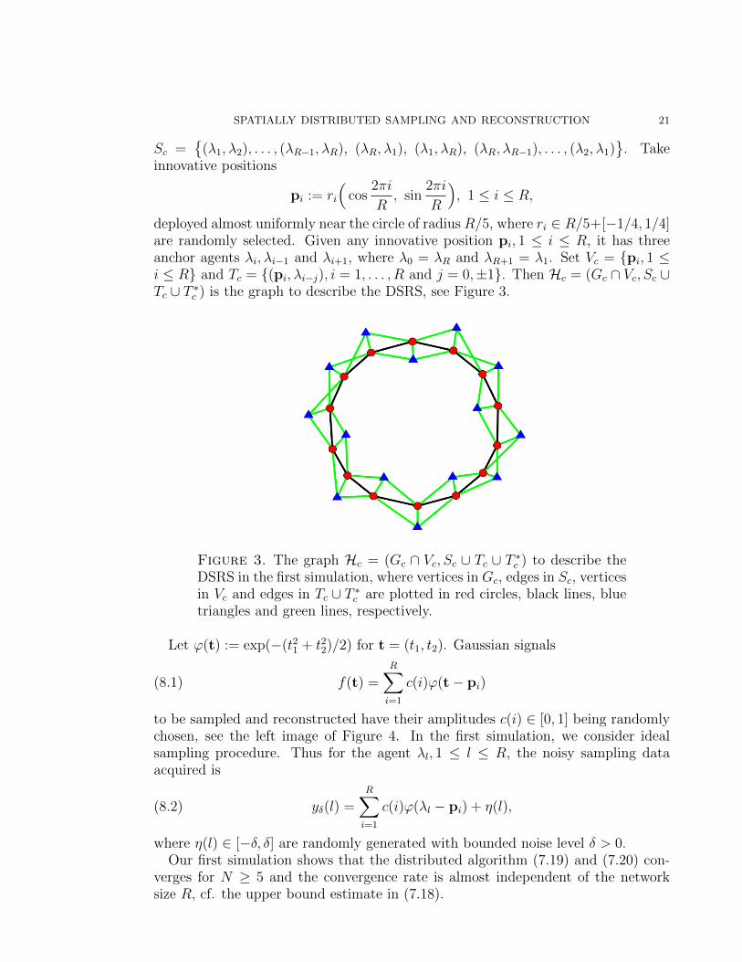
deployed almost uniformly near the circle of radius R/5, where ri ∈ R/5+[−1/4, 1/4]are randomly selected. Given any innovative position pi, 1 ≤ i ≤ R, it has threeanchor agents λi, λi−1 and λi+1, where λ0 = λR and λR+1 = λ1. Set Vc = {pi, 1 ≤i ≤ R} and Tc = {(pi, λi−j), i = 1, . . . , R and j = 0,±1}. Then Hc = (Gc ∩ Vc, Sc ∪Tc ∪ T ∗c ) is the graph to describe the DSRS, see Figure 3.

Figure 3. The graph Hc = (Gc ∩ Vc, Sc ∪ Tc ∪ T ∗c ) to describe theDSRS in the first simulation, where vertices in Gc, edges in Sc, verticesin Vc and edges in Tc ∪ T ∗c are plotted in red circles, black lines, bluetriangles and green lines, respectively.

Let ϕ(t) := exp(−(t21 + t22)/2) for t = (t1, t2). Gaussian signals

(8.1) f(t) =R∑i=1

c(i)ϕ(t− pi)

to be sampled and reconstructed have their amplitudes c(i) ∈ [0, 1] being randomlychosen, see the left image of Figure 4. In the first simulation, we consider idealsampling procedure. Thus for the agent λl, 1 ≤ l ≤ R, the noisy sampling dataacquired is

(8.2) yδ(l) =R∑i=1

c(i)ϕ(λl − pi) + η(l),

where η(l) ∈ [−δ, δ] are randomly generated with bounded noise level δ > 0.Our first simulation shows that the distributed algorithm (7.19) and (7.20) con-

verges for N ≥ 5 and the convergence rate is almost independent of the networksize R, cf. the upper bound estimate in (7.18).


Figure 4. Plotted on the left is the signal f in (8.1) with R = 80. Onthe right is the difference between the signal f and the reconstructedsignal fn,N,δ with n = 10, N = 6 and δ = 0.05.

Let fn,N,δ(t) :=∑R

i=1 cn,N,δ(i)ϕ(t − pi) be the reconstructed signal in the n-thiteration by applying the distributed algorithm (7.19) and (7.20) from the noisysampling data in (8.2), see the right image of Figure 4. Define maximal reconstruc-tion errors

ε(n,N, δ) :=

{max1≤i≤R |c(i)| if n = 0,max1≤i≤R |cn,N,δ(i)− c(i)| if n ≥ 1.

Presented in Table 1 is the average of reconstruction errors ε(n,N, δ) with 500 trialsin noiseless environment (δ = 0), where the network size R is 80. It indicates thatthe proposed distributed algorithm (7.19) and (7.20) has faster convergence ratefor larger N ≥ 5, and we only need three iteration steps to have a near perfectreconstruction from its noiseless samples when N = 10.

Table 1. Maximal reconstruction errors ε(n,N, δ) with δ = 0

HHHHHHn

N5 6 7 8 9 10

0 0.9874 0.9881 0.9878 0.9876 0.9877 0.98841 0.9875 0.4463 0.3073 0.1940 0.1055 0.05232 0.6626 0.2046 0.0794 0.0271 0.0124 0.00243 0.3624 0.0926 0.0240 0.0045 0.0014 0.00014 0.2535 0.0443 0.0068 0.0006 0.0001 0.00005 0.1742 0.0206 0.0018 0.0001 0.0000 0.00006 0.1169 0.0093 0.0005 0.0000 0.0000 0.00007 0.0840 0.0042 0.0001 0.0000 0.0000 0.00008 0.0579 0.0017 0.0000 0.0000 0.0000 0.00009 0.0411 0.0007 0.0000 0.0000 0.0000 0.000010 0.0289 0.0003 0.0000 0.0000 0.0000 0.0000

The robustness of the proposed algorithm (7.19) and (7.20) against samplingnoises is tested and confirmed, see Figure 4. Moreover, it is observed that the


maximal reconstruction error ε(n,N, δ) with large n depends almost linearly on thenoise level δ, cf. the sub-optimal approximation property in Theorem 5.4.

In the next simulation, agents are uniformly deployed on two concentric circlesand each agent has direct communication channels to its three adjacent agents.Then the graph Gp = (Gp, Sp) to describe our SDS is a prism graph with verticeshaving physical locations,

µl :=

{R10

(cos 4πθl

R, sin 4πθl

R

)if 1 ≤ l ≤ R

2(R10

+ 1)(

cos 4πθlR, sin 4πθl

R

)if R

2+ 1 ≤ l ≤ R,

where R ≥ 2 and θl ∈ l + [−1/4, 1/4], 1 ≤ l ≤ R, are randomly selected. Theinnovative positions

qi := ri(

cos4πi

R, sin

4πi

R

), 1 ≤ i ≤ R

2,

have four anchor agents µi, µi+1, µi+R/2 and µi+R/2+1, where µ0 = µR/2, µR+1 =

µR/2+1, and ri ∈ R10

+ [14, 3

4] are randomly selected. Set Vp = {qi, 1 ≤ i ≤ R

2}

and Tp = {(qi, µi+j), i = 1, . . . , R2

and j = 0, 1, R2, R

2+ 1}. Thus the graph Hp =

(Gp ∩ Vp, Sp ∪ Tp ∪ T ∗p ) to describe our DSRS is a connected simple graph, see theleft image of Figure 5.

Figure 5. Plotted on the left is the graphHp = (Gp∩Vp, Sp∪Tp∪T ∗p )to describe the DSRS, where vertices in Gp and Vp are in red circlesand blue triangles, and edges in Sp and Tp ∪ T ∗p are in black solidlines and green solid lines, respectively. On the right is a subgraph ofHp, where some agents are completely dysfunctional and some havecommunication channels to one or two of their nearby agents clogged.

Following the first simulation, we consider the ideal sampling procedure of signals,

(8.3) g(t) =

R/2∑i=1

d(i)ϕ(t− qi),

where d(i) ∈ [0, 1], 1 ≤ i ≤ R/2, are randomly selected, see the left image of Figure6. Then the noisy sampling data acquired by the agent µl, 1 ≤ l ≤ R, is


Figure 6. Plotted on the left is the signal g in (8.3) with R = 160.On the right is the difference between the signal g and its approxima-tion gn,N,δ, where n = 4, N = 6, δ = 0.05, and agents located at µ1, µ87

are completely dysfunctional, while agents located at µ11, µ51, µ91 havetheir partial communication channels clogged.

(8.4) yδ(l) =

R/2∑i=1

d(i)ϕ(µl − qi) + η(l),

where η(l) ∈ [−δ, δ] are randomly selected with bounded noise level δ > 0. Applyingthe distributed algorithm (7.19) and (7.20), we obtain approximations

(8.5) gn,N,δ(t) =

R/2∑i=1

dn,N,δ(i)ϕ(t− qi), n ≥ 1,

of the signal g in (8.3). Our simulations illustrate that the distributed algorithm(7.19) and (7.20) converges for N ≥ 3 and the signal g can be reconstructed nearperfectly from its noiseless samples in 12 steps for N = 3, 7 steps for N = 4, 5steps for N = 5, 4 steps for N = 6, and 3 steps for N = 7, cf. Table 1 in the firstsimulation.

The robustness of the proposed distributed algorithm (7.19) and (7.20) againstsampling noises and dysfunctions of agents in the DSRS is tested and confirmed, seethe right graph of Figure 5 and the right image of Figure 6.

9. Proofs

In this section, we include proofs of Propositions 2.4, 3.1, 3.2, 3.3, 3.4, 4.1, 4.2,7.1, and Theorems 5.2, 5.3, 5.4, 6.1, 6.2, 7.2.

9.1. Proof of Proposition 2.4. For any λ ∈ G, take λm ∈ GN with BG(λ,N) ∩BG(λm, N) 6= ∅. Then

ρG(λ, λm) ≤ ρG(λ, λ′) + ρG(λ

′, λm) ≤ 2N,


where λ′ is a vertex in BG(λ,N) ∩ BG(λm, N). This proves that for any N ′ ≥ 2N ,balls {BG(λm, N ′), λm ∈ GN} provide a covering for G,

(9.1) G ⊂⋃

λm∈GN

BG(λm, N′),

and hence the first inequality in (2.9) follows.Now we prove the last inequality in (2.9). Take λ ∈ G. For any λm, λm′ ∈

GN ∩BG(λ,N ′),

ρG(λ′, λm′) ≤ ρG(λ

′, λm) + ρG(λm, λ) + ρG(λ, λm′) ≤ 2N ′ +N

for all λ′ ∈ B(λm, N), which implies that

(9.2) BG(λm, N) ⊂ BG(λm′ , 2N′ +N).

Hence∑λm∈GN

χBG(λm,N ′)(λ)≤µG(∪λm∈GN∩BG(λ,N ′)BG(λm, N))

infλm∈GN∩BG(λ,N ′) µG(BG(λm, N))

≤ supλm∈GN∩BG(λ,N ′)

µG(BG(λm, 2N′ +N))

µG(BG(λm, N))≤ (D0(G))dlog2(2N ′/N+1)e,(9.3)

where the first inequality holds as BG(λm, N), λm ∈ VN , are disjoint, the second oneis true by (9.2), and the third inequality follows from the doubling assumption (2.1).

9.2. Proof of Proposition 3.1. By the structure of the graph H, it suffices toshow that the shortest path in H to connect distinct vertices λ, λ′ ∈ G must be apath in its subgraph G. Suppose on the contrary that λu1 · · ·uk−1ukuk+1 · · ·unλ′ isa shortest path in H of length ρH(λ, λ′) with vertex uk along the path belonging toV . Then uk−1 and uk+1 are anchor agents of uk in G.

For the case that uk−1 and uk+1 are distinct anchor agents of the innovativeposition uk, (uk−1, uk+1) ∈ S by (3.1). Hence λu1 · · ·uk−1uk+1 · · ·unλ′ is a path oflength ρH(λ, λ′)− 1 to connect vertices λ and λ′, which is a contradiction.

Similarly for the case that uk−1 and uk+1 are the same, λu1 · · ·uk−1uk+2 · · ·unλ′ isa path of length ρH(λ, λ′)− 2 to connect vertices λ and λ′. This is a contradiction.

9.3. Proof of Proposition 3.2. The non-negativity and symmetry is obvious,while the identity of indiscernibles holds since there is no edge assigned inH betweentwo distinct vertices in V .

Now we prove the triangle inequality

(9.4) ρ(i, i′) ≤ ρ(i, i′′) + ρ(i′′, i′) for distinct vertices i, i′, i′′ ∈ V.

Let m = ρ(i, i′′) and n = ρ(i′′, i′). Take a path iv1 . . . vmi′′ of length m + 1 to

connect i and i′′, and another path i′′u1 . . . uni′ of length n+ 1 to connect i′′ and i′.

If vm = u1, then iv1 . . . vmu2 · · ·uni′ is a path of length m + n to connect vertices iand i′, which implies that

(9.5) ρ(i, i′) ≤ m+ n− 1 < ρ(i, i′′) + ρ(i′′, i′).


If vm 6= u1, then (vm, u1) is an edge in the graph G (and then also in the graph H)by (3.1). Thus iv1 . . . vmu1u2 · · ·uni′ is a path of length m+n+1 to connect verticesi and i′, and

(9.6) ρ(i, i′) ≤ m+ n = ρ(i, i′′) + ρ(i′′, i′).

Combining (9.5) and (9.6) proves (9.4).

9.4. Proof of Proposition 3.3. To prove Proposition 3.3, we need two lemmascomparing measures of balls in graphs G and V .

Lemma 9.1. If H satisfies (3.1) and (3.2), then

(9.7) µ(B(i, r)) ≤ LµG(BG(λ, r)) for any λ ∈ G with (i, λ) ∈ T.

Proof. Let i′ ∈ B(i, r) with i′ 6= i. By Proposition 3.1, there exists a path λ1 . . . λnof length ρ(i, i′)− 1 in the graph G such that (i, λ1), (i′, λn) ∈ T . Then

ρG(λ, λn) ≤ ρG(λ, λ1) + ρG(λ1, λn) ≤ ρ(i, i′) ≤ r

as either λ1 = λ or (λ, λ1) is an edge in G by (3.1). This shows that for anyinnovative position i′ ∈ B(i, r) there exists an anchor agent λn in the ball BG(λ, r).This observation together with (3.2) proves (9.7). �

Lemma 9.2. If H satisfies (2.3), (3.1) and (3.3), then

(9.8) µG(BG(λ, r)) ≤(

supλ′∈G

µG(BG(λ′, 2M + 2))

)µ(B(i, r +M + 1))

for any λ ∈ G and r ≥M + 1, where (i, λ′) ∈ T and λ′ ∈ BG(λ,M).

Proof. Let λ1 = λ and take Λ = {λm}m≥1 such that (i) BG(λm,M+1) ⊂ BG(λ, r) forall λm ∈ Λ; (ii) BG(λm,M+1)

⋂BG(λm′ ,M+1) = ∅ for all distinct vertices λm, λm′ ∈

Λ; and (iii) BG(λ,M+1)⋂(⋃

λm∈ΛBG(λm,M+1))6= ∅ for all λ ∈ BG(λ, r). The set

Λ could be considered as a maximal (M + 1)-disjoint subset of BG(λ, r). Followingthe argument used in the proof of Proposition 2.4, {BG(λm, 2(M + 1))}λm∈Λ formsa covering of the ball B(λ, r), which implies that(9.9)

µG(BG(λ, r)) ≤(

supλm∈Λ

µG(BG(λm, 2M + 2)))

#Λ ≤(

supλ′∈G

µG(BG(λ′, 2M + 2))

)#Λ.

For λm ∈ Λ, define

Vλm = {i′ ∈ V, (i′, λ) ∈ T for some λ ∈ BG(λm,M)}.

Then it follows from (3.3) that

(9.10) #Vλm ≥ 1 for all λm ∈ Λ.

Observe that the distance of anchor agents associated with innovative positions indistinct Vλm is at least 2 by the second requirement (ii) for the set Λ. This togetherwith the assumption (3.1) implies that

(9.11) Vλm ∩ Vλm′ = ∅ for distinct λm, λm′ ∈ Λ.


Combining (9.9), (9.10) and (9.11) leads to

(9.12) µG(BG(λ, r)) ≤(

supλ′∈G

µG(BG(λ′, 2M + 2))

)#(∪λm∈Λ Vλm

).

Take i ∈ V with (i, λ′) ∈ T for some λ′ ∈ BG(λ,M), and i′ ∈ Vλm , λm ∈ Λ. Then

ρH(i, λ) ≤ ρH(i, λ′) + ρH(λ′, λ) ≤M + 1,

and

ρH(i′, λ) ≤ ρH(i′, λ) + ρH(λ, λ) ≤ r + 1,

where λ ∈ BG(λm,M) and (i′, λ) ∈ T . Thus

(9.13) ρ(i, i′) ≤ r +M + 1.

Then the desired estimate (9.8) follows from (9.12) and (9.13). �

We are ready to prove Proposition 3.3.

Proof of Proposition 3.3. First we prove the doubling property (3.10) for the mea-sure µ. Take i ∈ V . Then for r ≥ 2(M + 1) it follows from Lemmas 9.1 and 9.2that

µ(B(i, 2r)) ≤ LµG(BG(λ, 2r)) ≤ L(D0(G))2µG(BG(λ, r/2))

≤ KL(D0(G))2µ(B(i, r/2 +M + 1)) ≤ KL(D0(G))2µ(B(i, r)),(9.14)

where λ ∈ G is a vertex with (i, λ) ∈ T and

(9.15) K := supλ′∈G

µG(BG(λ′, 2M + 2)) ≤ ((deg(G))2M+3 − 1

deg(G)− 1

by (2.6). From the doubling property (2.1) for the measure µG, we obtain

(9.16) µ(B(i, 2r)) ≤ KLD0(G) ≤ KLD0(G)µ(B(i, r)) for 0 ≤ r ≤ 2(M + 1).

Then the doubling property (3.10) follows from (9.14), (9.15) and (9.16).Next we prove the doubling property (3.11) for the measure µG. Let λ′ ∈ BG(λ,M)

with (i, λ′) ∈ T for some i ∈ V . The existence of such λ′ follows from assumption(3.3). From Lemmas 9.1 and 9.2, we obtain

µG(BG(λ, 2r)) ≤ Kµ(B(i, 2r +M + 1)) ≤ D20Kµ

(B(i,r

2+

(M + 1)

4

))≤ D2

0LKµG

(BG

(λ′,

r

2+M + 1

4

))≤ D2

0LKµG

(BG

(λ,r

2+M + 1

4+M

))≤ D2

0LKµG(BG(λ, r))(9.17)

for r ≥ 3M , and

µG(BG(λ, 2r)) ≤ Kµ(B(i, 7M)) ≤ D20Kµ(B(i, 2M))

≤ D20LKµG(BG(λ

′, 2M)) ≤ D20LK

2µG(BG(λ, r))(9.18)

for 0 ≤ r ≤ 3M − 1. Combining (9.15), (9.17) and (9.18) proves (3.11). �


9.5. Proof of Proposition 3.4. The polynomial growth property (3.12) for themeasure µ follows immediately from Lemma 9.1.

The polynomial growth property (3.13) for the measure µG holds because

µG(BG(λ, r)) ≤(deg(G))M − 1

deg(G)− 1, 0 ≤ r ≤M − 1

by (2.6), and

µG(BG(λ, r)) ≤ D1

((deg(G))2M+3 − 1

deg(G)− 1

)(r +M + 2)d

≤ 2dD1

((deg(G))2M+3 − 1

deg(G)− 1

)(r + 1)d, r ≥M,

by (9.15) and Lemma 9.2.

9.6. Proof of Proposition 4.1. To prove Proposition 4.1, we need a lemma.

Lemma 9.3. Let G be a connected simple graph. If its counting measure has poly-nomial growth (2.4), then

(9.19) supλ∈G

∑ρG(λ,λ′)≥s

(1 + ρG(λ, λ′))−α ≤ D1(G)α

α− d(s+ 1)−α+d

for all α > d and nonnegative integers s, where d and D1(G) are the Beurlingdimension and sampling density respectively.

Proof. Take λ ∈ G and α > d. Then∑ρG(λ,λ′)≥s

(1 + ρG(λ, λ′))−α =

∑n≥s

(n+ 1)−α( ∑ρG(λ,λ′)=n

1)

≤∑n≥s

µG(BG(λ, n))((n+ 1)−α − (n+ 2)−α)

≤ D1(G)∞∑n=s

(n+ 1)d((n+ 1)−α − (n+ 2)−α)

= D1(G)(

(s+ 1)−α+d +∞∑

n=s+1

(n+ 1)−α((n+ 1)d − nd

))≤ D1(G)

((s+ 1)−α+d + d

∫ ∞s+1

td−α−1dt)

=D1(G)α

α− d(s+ 1)−α+d,(9.20)

where the second inequality follows from (2.4), and the third one is true as (n +1)d − nd ≤ d(n+ 1)d−1 for n ≥ 1 and d ≥ 1. �

Now we prove Proposition 4.1.


Proof of Proposition 4.1. Take A ∈ Jα(G,V) and c := (c(i))i∈V ∈ `p, 1 < p < ∞.Then

‖Ac‖pp ≤ ‖A‖pJα(G,V)

∑λ∈G

(∑i∈V

(1 + ρH(λ, i))−α|c(i)|)p

≤ ‖A‖pJα(G,V)‖c‖pp

(supλ′∈G

∑i′∈V

(1 + ρH(λ′, i′))−α)p−1(

supi′∈V

∑λ′∈G

(1 + ρH(λ′, i′))−α).(9.21)

For any λ′ ∈ G and i′ ∈ V , it follows from Proposition 3.1 that

(9.22) ρG(λ′, λ′′) + 1 ≥ ρH(λ′, i′) ≥ ρG(λ

′, λ′′) for all λ′′ ∈ G with (i′, λ′′) ∈ T.

By (3.2), (3.14), (9.22) and Lemma 9.3, we obtain∑i′∈V

(1 + ρH(λ′, i′))−α≤∑λ′′∈G

( ∑(i′,λ′′)∈T

1)

(1 + ρG(λ′, λ′′))−α

≤ L∑λ′′∈G

(1 + ρG(λ′, λ′′))−α ≤ LD1(G)α

α− dfor any λ′ ∈ G,(9.23)

and

(9.24)∑λ′∈G

(1 + ρH(λ′, i′))−α ≤∑λ′∈G

(1 + ρG(λ′, λ′′))−α ≤ D1(G)α

α− dfor any i′ ∈ V,

where λ′′ ∈ G satisfies (i′, λ′′) ∈ T . Combining (9.21), (9.23) and (9.24) proves (4.4)for 1 < p <∞.

We can use similar argument to prove (4.4) for p = 1,∞. �

9.7. Proof of Proposition 4.2. Following the proof of Proposition 4.1, we obtain

‖(A−As)c‖p ≤ ‖A‖Jα(G,V)

(supλ′∈G

∑ρH(λ′,i′)>s

(1 + ρH(λ′, i′))−α)1−1/p

×(

supi′∈V


(1 + ρH(λ′, i′))−α)1/p

‖c‖p,(9.25)

where c ∈ `p, 1 ≤ p ≤ ∞. Applying similar argument used to prove (9.19), (9.23)and (9.24), we have(9.26)

supλ′∈G


(1+ρH(λ′, i′))−α ≤ L supλ′∈G

∑ρG(λ′,λ′′)≥s

(1+ρG(λ′, λ′′))−α ≤ D1(G)Lα

α− d(s+1)−α+d

and

(9.27) supi′∈V


(1 + ρH(λ′, i′))−α ≤ D1(G)α

α− d(s+ 1)−α+d.

Then the approximation error estimate (4.6) follows from (9.25), (9.26) and (9.27).


9.8. Proof of Theorem 5.3. To prove Wiener’s lemma (Theorem 5.3) for Jα(V), α >d, we first show that it is a Banach algebra of matrices.

Proposition 9.4. Let V be an undirected graph with the counting measure µ havingpolynomial growth (3.9). Then for any α > d, Jα(V) is a Banach algebra of matrices:

(i) ‖βC‖Jα(V) = |β|‖C‖Jα(V);(ii) ‖C + D‖Jα(V) ≤ ‖C‖Jα(V) + ‖D‖Jα(V);

(iii) ‖CD‖Jα(V) ≤ 2α+1D1αα−d ‖C‖Jα(V)‖D‖Jα(V); and

(iv) ‖Dc‖2 ≤ D1αα−d‖D‖Jα(V)‖c‖2

for any scalar β, vector c ∈ `2 and matrices C,D ∈ Jα(V).

Proof. The first two conclusions follow immediately from (5.2) and (5.3).Now we prove the third conclusion. Take C,D ∈ Jα(V). Then

‖CD‖Jα(V) ≤ 2α‖C‖Jα(V)‖D‖Jα(V) supi,i′∈V

( ∑ρ(i,i′′)≥ρ(i,i′)/2

(1 + ρ(i′′, i′))−α

+∑

ρ(i′′,i′)≥ρ(i,i′)/2

(1 + ρ(i, i′′))−α).(9.28)

Following the argument used in the proofs of Lemma 9.3, we have

(9.29) supi∈V

∑ρ(i,i′)≥s

(1 + ρ(i, i′))−α ≤ D1α

α− d(s+ 1)−α+d, 0 ≤ s ∈ Z.

Combining (9.28) and (9.29) proves the third conclusion.Following the proof of Proposition 4.1 and applying (9.29) instead of (9.23) and

(9.24), we obtain the fourth conclusion. �

Now, we prove Theorem 5.3.

Proof of Theorem 5.3. Following the argument in [58], it suffices to establish thefollowing differential norm inequality:

(9.30) ‖C2‖Jα(V) ≤ 2α+d/2+2D1/21 (D1α/(α− d))1−θ(‖C‖Jα(V))

2−θ(‖C‖B2)θ

holds for all C ∈ Jα(V), where θ = (2α− 2d)/(2α− d) ∈ (0, 1).Write C = (c(i, i′))i,i′∈V . Then

‖C2‖Jα(V) ≤ 2α‖C‖Jα(V)

(supi,i′∈V

∑ρ(i,i′′)≥ρ(i,i′)/2

|c(i′′, i′)|+ supi,i′∈V

∑ρ(i′′,i′)≥ρ(i,i′)/2

|c(i, i′′)|)

≤ 2α‖C‖Jα(V)

(supi′∈V

∑i′′∈V

|c(i′′, i′)|+ supi∈V

∑i′′∈V

|c(i, i′′)|).(9.31)

Set

(9.32) τ :=(D1α‖C‖Jα(V)

(α− d)‖C‖B2

)2/(2α−d)

≥ 1


by Proposition 9.4. For i′ ∈ V , we obtain∑i′′∈V

|c(i′′, i′)| ≤( ∑ρ(i′′,i′)≤τ

|c(i′′, i′)|2)1/2( ∑

ρ(i′′,i′)≤τ

1)1/2

+ ‖C‖Jα(V)

∑ρ(i′′,i′)>τ

(1 + ρ(i′′, i′))−α

≤D1/21 ‖C‖B2(1 + bτc)d/2 +D1α(α− d)−1‖C‖Jα(V)(1 + bτc)−α+d

≤ 2d/2+1D1/21 (D1α/(α− d))d/(2α−d)(‖C‖Jα(V))

1−θ(‖C‖B2)θ,(9.33)

where the second inequality holds by (9.29) and the last inequality follows from(9.32). Similarly, for i ∈ V we have

(9.34)∑i′′∈V

|c(i′, i′′)| ≤ 2d/2+1D1/21 (D1α/(α− d))d/(2α−d)(‖C‖Jα(V))

1−θ(‖C‖B2)θ.

Combining (9.31), (9.33) and (9.34) proves (9.30). This completes the proof ofTheorem 5.3. �

9.9. Proof of Theorem 5.2. To prove Theorem 5.2, we need Theorem 5.3 and thefollowing lemma about families Jα(G,V) and Jα(V) of matrices.

Lemma 9.5. Let G,H,V and d be as in Proposition 5.1. Then

(i) ‖AC‖Jα(G,V) ≤ 2α+1LD1(G)αα−d ‖A‖Jα(G,V)‖C‖Jα(V) for all A ∈ Jα(G,V) and C ∈

Jα(V).

(ii) ‖ATB‖Jα(V) ≤ 2α+1D1(G)αα−d ‖A‖Jα(G,V)‖B‖Jα(G,V) for all A,B ∈ Jα(G,V).

Proof. Take A ∈ Jα(G,V) and C ∈ Jα(V). Observe from (3.1) that

ρH(λ, i) ≤ ρH(λ, i′) + ρ(i′, i) for all λ ∈ G and i, i′ ∈ V.

Similar to the argument used in the proof of Proposition 9.4, we obtain

‖AC‖Jα(G,V) ≤ 2α‖A‖Jα(G,V)‖C‖Jα(V)

(supi∈V

∑i′∈V

(1+ρ(i′, i))−α+supλ∈G

∑i′∈V

(1+ρH(λ, i′))−α).

This together with (3.15), (9.26) and (9.29) proves the first conclusion.Recall that

(9.35) ρ(i, i′) ≤ ρH(λ, i) + ρH(λ, i′) for all λ ∈ G and i, i′ ∈ V.

Then for A,B ∈ Jα(G,V), we obtain from (9.27) and (9.35) that

‖ATB‖Jα(V) ≤ 2α+1‖A‖Jα(G,V)‖B‖Jα(G,V) supi∈V

∑λ∈G

(1 + ρH(λ, i))−α

≤ 2α+1D1(G)α

α− d‖A‖Jα(G,V)‖B‖Jα(G,V).

This completes the proof of the second conclusion. �

Now we prove Theorem 5.2.


Proof of Theorem 5.2. Take A ∈ Jα(G,V) that has `2-stability. Then ATA hasbounded inverse on `2. Observe that ATA ∈ Jα(V) by Lemma 9.5. Therefore(ATA)−1 ∈ Jα(V) and A(ATA)−1 ∈ Jα(G,V) by Theorem 5.3 and Lemma 9.5.Hence for any c ∈ `p,

‖c‖p = ‖(ATA)−1ATAc‖p ≤D1(G)Lα

α− d‖A(ATA)−1‖Jα(G,V)‖Ac‖p

and

‖Ac‖p ≤D1(G)Lα

α− d‖A‖Jα(G,V)‖c‖p

by Proposition 4.1 and the dual property between sequences `p and `p/(p−1). The`p-stability for the matrix A then follows. �

9.10. Proof of Theorem 5.4. The conclusion (5.4) follows immediately from Propo-sition 4.1, Theorem 5.3 and Lemma 9.5.

9.11. Proof of Theorem 6.1. Observe from Proposition 3.1 that

BH(γ, r) ∩G = {γ′ ∈ G, ρG(γ, γ′) ≤ r}, γ ∈ G.

and

BH(i, r) ∩ V = {i′ ∈ V, ρ(i, i′) ≤ max(r − 1, 0)}, i ∈ V.Take c = (c(i))i∈V supported in BH(λ,N) ∩ V and write Ac = (d(λ′))λ′∈G. Then

(9.36) ‖Ac‖2 ≥ A‖A‖Jα(G,V)‖c‖2

and ∑ρH(λ′,λ)>2N

|d(λ′)|2 ≤ LD1(G)N−α+d‖A‖2Jα(G,V)

×∑

ρH(λ′,λ)>2N

∑i∈BH(λ,N)∩V

(1 + ρH(λ′, i))−α|c(i)|2

≤(D1(G)

)2LN−2α+2dα(α− d)−1‖A‖2

Jα(G,V)‖c‖22,(9.37)

where the first inequality holds as

ρH(λ′, i′) ≥ ρH(λ′, λ)− ρH(i′, λ) > N

for all λ′ 6∈ BH(λ, 2N) and i′ ∈ BH(λ,N), and the last inequality follows from (9.27).Combining (9.36) and (9.37) proves (6.1).

9.12. Proof of Theorem 6.2. In this subsection, we will prove the following strongversion of Theorem 6.2.

Theorem 9.6. Let G,H,V and A be as in Theorem 6.2. If there exists a positiveconstant A0, an integer N0 ≥ 3, and a maximal N0

4-disjoint subset GN0/4 such that

(6.3) is true and (6.4) hold for all λm ∈ GN0/4, then A satisfies (6.5).


Proof. Let ψ0 be the trapezoid function,

(9.38) ψ0(t) =

1 if |t| ≤ 1/22− 2|t| if 1/2 < |t| ≤ 10 if |t| > 1.

For λ ∈ G, define multiplication operators ΨNλ,V and ΨN

λ,G by

(9.39) ΨNλ,V : (c(i))i∈V 7−→

(ψ0(ρH(λ, i)/N)c(i)

)i∈V ,

(9.40) ΨNλ,G : (d(λ′))λ′∈G 7−→

(ψ0(ρH(λ, λ′)/N)d(λ′)

)λ′∈G.

Observe that

ANΨNλ,V = ANχ

Nλ,V ΨN

λ,V = χ2Nλ,GANχ

Nλ,V ΨN

λ,V , N ≥ 0,

where AN is a band approximation of the matrix A in (4.5). Then for all λm ∈ GN0/4,it follows from Proposition 4.2 and our local stability assumption (6.4) that

‖AN0ΨN0λm,V

c‖2 ≥ ‖χ2N0λm,G

AχN0λm,V

ΨN0λm,V

c‖2 − ‖χ2N0λm,G

(A−AN0)ΨN0λm,V

c‖2

≥(A0 −

D1(G)Lα

α− dN−α+d

0

)‖A‖Jα(G,V)‖ΨN0

λm,Vc‖2, c ∈ `2.

Therefore ( ∑λm∈GN0/4

‖AN0ΨN0λm,V

c‖22

)1/2

≥(A0 −

D1(G)Lα

α− dN−α+d

0

)‖A‖Jα(G,V)

( ∑λm∈GN0/4

‖ΨN0λm,V

c‖22

)1/2

≥(A0

3− D1(G)Lα

3(α− d)N−α+d

0

)‖A‖Jα(G,V)‖c‖2,(9.41)

where the last inequality holds because for all i ∈ V ,

∑λm∈GN0/4

|ψ0(ρH(λm, i)/N0)|2 ≥(N0 − 2

N0

)2 ∑λm∈GN0/4

χBH(λm,N0/2+1)(i) ≥1

9

by (9.38), Proposition 2.4 and the assumption that N0 ≥ 3.Next, we estimate commutators

AN0ΨN0λm,V

−ΨN0λm,G

AN0 = (AN0ΨN0λm,V

−ΨN0λm,G

AN0)χ2N0λm,V

, λm ∈ GN0/4.


Take c = (c(i))i∈V ∈ `2. Then∑λm∈GN0/4

‖(AN0ΨN0λm,V

−ΨN0λm,G

AN0)c‖22

≤ ‖A‖2Jα(G,V)

∑λm∈GN0/4

∑λ∈G

{ ∑ρH(λ,i)≤N0

(1 + ρH(λ, i))−α

×∣∣∣ψ0

(ρH(λ, λm)

N0

)− ψ0

(ρH(i, λm)

N0

)∣∣∣χBH(λm,2N0)∩V (i)|c(i)|}2

≤ 4(D0(G))4N−20 ‖A‖2

Jα(G,V)

(supi∈V

∑λ∈BH(i,N0)∩G

(1 + ρH(λ, i))−αρH(λ, i))

×(

supλ∈G

∑i∈BH(λ,N0)∩V

(1 + ρH(λ, i))−αρH(λ, i))‖c‖2

2,(9.42)

where the last inequality follows from Propositions 2.4 and 3.1, and

|ψ0(t)− ψ0(t′)| ≤ 2|t− t′| for all t, t′ ∈ R.

Following the argument used in (9.19), we have

supi∈V

∑λ∈BH(i,N0)∩G

(1 + ρH(λ, i))−αρH(λ, i)

≤ supλ′∈G

∑ρG(λ,λ′)≤N0

(1 + ρG(λ, λ′))−α+1

≤ D1(G)(N0 + 1)−α+d+1 + (α− 1)D1(G)

N0−1∑n=0

(n+ 1)−α+d

≤ D1(G)(N0 + 1)−α+d+1 +D1(G)(α− 1)(

1 +

∫ N0

1

t−α+ddt)

≤

D1(G)(α−1)(α−d)

α−d−1if α > d+ 1

D1(G)(1 + d+ d lnN0) if α = d+ 12d+1−αD1(G)d

d+1−α Nd+1−α0 if α < d+ 1

(9.43)

and

supλ∈G

∑i∈BH(λ,N0)∩V

(1 + ρH(λ, i))−αρH(λ, i)

≤ L supλ∈G

∑λ′∈BG(λ,N0)

(1 + ρG(λ, λ′))−α+1

≤

D1(G)L(α−1)(α−d)

α−d−1if α > d+ 1

D1(G)L(1 + d+ d lnN0) if α = d+ 12d+1−αD1(G)dL

d+1−α Nd+1−α0 if α < d+ 1.

(9.44)


Therefore,

(D0(G))2‖AN0c‖2 ≥( ∑λm∈GN0/4

‖ΨN0λm,G

AN0c‖22

)1/2

≥( ∑λm∈GN0/4

‖AN0ΨN0λm,V

c‖22

)1/2

−( ∑λm∈GN0/4

‖(AN0ΨN0λm,V

−ΨN0λm,G

AN0)c‖22

)1/2

≥A0‖A‖Jα(G,V)

3‖c‖2 −D1(G)L‖A‖Jα(G,V)N

−min(α−d,1)0 ‖c‖2

×

(

α3(α−d)

+ 2(D0(G))2(α−1)(α−d)α−d−1

)if α > d+ 1(

d+13

+ 2(D0(G))2(1 + d+ d lnN0))

if α = d+ 1(α

3(α−d)+ 4(D0(G))2d

d+1−α

)if α < d+ 1,

where the first inequality holds by Proposition 2.4, and the third inequality followsfrom (9.41) and (9.42). This together with Proposition 4.2 completes the proof. �

9.13. Proof of Proposition 7.1. To prove Proposition 7.1, we need the followingcritical estimate.

Proposition 9.7. Let G, H, V and S be as in Proposition 7.1. Then

(9.45) ‖(χNλ,V STSχNλ,V )−1‖Jα(V) ≤2−α−1(α− d)2D2


,

where D2 is the constant in (7.8).

Proof. Let Jλ,N := χNλ,V STSχNλ,V . By Lemma 9.5, we have

‖Jλ,N‖Jα(V) ≤2α+1D1(G)α

α− d‖S‖2

Jα(G,V).(9.46)

This together with Propositions 9.4 implies that

A2‖S‖2Jα(G,V)‖χNλ,V x‖2

2 ≤ ‖SχNλ,V x‖22 = 〈Jλ,Nx,x〉 ≤ 2α+1α2D1D1(G)

(α− d)2‖S‖2

Jα(G,V)‖χNλ,V x‖22

for all x ∈ `2. Hence

(9.47) Jλ,N =2α+1α2D1D1(G)

(α− d)2‖S‖2

Jα(G,V)(IBH(λ,N)∩V −Bλ,N)

for some Bλ,N satisfying

(9.48) ‖Bλ,N‖B2 ≤ r0

and(9.49)

‖Bλ,N‖Jα(V) ≤ ‖IBH(λ,N)∩V ‖Jα(V) +2−α−1(α− d)2‖Jλ,N‖Jα(V)


≤ 1 +α− dαD1

≤ 2,


where IBH(λ,N)∩V is the identity matrix on BH(λ,N) ∩ V . Then following the argu-ment in [58] and applying (9.30) with C replaced by Bλ,N and V by BH(λ,N)∩ V ,we obtain the following estimate

‖(Bλ,N)n‖Jα(V) ≤(D 1

1−θ ‖Bλ,N‖Jα(V)

‖Bλ,N‖B2

) 2−θ1−θn

log2(2−θ)

‖Bλ,N‖nB2 for all n ≥ 1,

where D = 22α+d/2+3D1/21 (D1α/(α − d))2−θ. This together with (9.48) and (9.49)

leads to

(9.50) ‖(Bk,N)n‖Jα(V) ≤ (2D1

1−θ /r0)2−θ1−θn

log2(2−θ)rn0 for all n ≥ 1.

Observe that

(9.51) ‖(Jλ,N)−1‖Jα(V) ≤2−α−1(α− d)2


(1 +

∞∑n=1

‖(Bλ,N)n‖Jα(V)

)by (9.47). Combining (9.50) and (9.51) completes the proof. �

Proof of Proposition 7.1. Observe from (7.2) and (7.3) that

χN/2λ,V (dλ,N − d2) = χ

N/2λ,V (χNλ,V STSχNλ,V )−1χNλ,V STS(I− χNλ,V )d2.

This together with (9.29), Lemma 9.5, and Propositions 9.4 and 9.7 implies that

‖χN/2λ,V (dλ,N − d2)‖∞ ≤ ‖(χNλ,V STSχNλ,V )−1χNλ,V STS‖Jα(V) ×(sup

i∈BH(λ,N/2)∩V

∑j /∈BH(λ,N)∩V

(1 + ρH(i, j))−α)‖d2‖∞

≤ 2α+1D1α

α− d‖(χNλ,V STSχNλ,V )−1‖Jα(V)‖STS‖Jα(V) ×(

supi∈V

∑ρH(i,j)>N/2

(1 + ρH(i, j))−α)‖d2‖∞

≤ 2α+1D2

(supi∈V

∑ρH(i,j)>N/2

(1 + ρH(i, j))−α)‖d2‖∞

≤ 2α+1D1D2α

α− d

(N2

+ 1)−α+d

‖d2‖∞ ≤ D3(N + 1)−α+d‖d2‖∞.

This proves the estimate (7.6).Now we prove (7.7). Set yLS = (STS)−1d2. By (9.29),

(9.52) ‖yLS‖∞ ≤D1α

α− d‖(STS)−1‖Jα(V)‖d2‖∞.

Moreover, following the proof of Proposition 9.7 gives

(9.53) ‖(STS)−1‖Jα(V) ≤2−α−1(α− d)2D2


.


Write

χN/2λ,G (wλ,N −wLS) = χ

N/2λ,G (χNλ,GSχNλ,V )(χNλ,V STSχNλ,V )−2χNλ,V STS(I − χNλ,V )d2

+χN/2λ,G (χNλ,GSχNλ,V )(χNλ,V STSχNλ,V )−1χNλ,V STS(I − χNλ,V )yLS

−χN/2λ,GS(I − χNλ,V )yLS

=: I + II + III.(9.54)

Using (9.26), (9.52), (9.53), Lemma 9.5, and Propositions 9.4 and 9.7, we obtain

‖I‖∞ ≤ ‖(χNλ,GSχNλ,V )(χNλ,V STSχNλ,V )−2χNλ,V STS‖Jα(G,V) ×(sup

λ′∈BH(λ,N/2)∩G

∑i/∈BH(λ,N)∩V

(1 + ρH(λ′, i))−α)‖d2‖∞

≤ 22α+2LD22

‖S‖Jα(G,V)

(supλ′∈G

∑ρH(λ′,i)>N/2

(1 + ρH(λ′, i))−α)‖d2‖∞

≤ 23α−d+2αL2D1(G)D22

(α− d)‖S‖Jα(G,V)

(N + 1)−α+d‖d2‖∞,

‖II‖∞ ≤ 23α−d+2α2L2(D1(G))2D2

(α− d)2‖S‖Jα(G,V)(N + 1)−α+d‖yLS‖∞

≤ 22α−d+1αL2D1(G)D22

(α− d)‖S‖Jα(G,V)

(N + 1)−α+d‖d2‖∞,

and

‖III‖∞ ≤ LD2

‖S‖Jα(G,V)

(N + 1)−α+d‖d2‖∞.

These together with (9.54) prove (7.7). �

9.14. Proof of Theorem 7.2. Let

(9.55) un = ST (wn −wLS) = STwn − d2 and vn = Sun, n ≥ 1.

Then,

un+1 = un − STRNSTSun = ST(S(STS)−2STvn −RNSTvn

)by (7.13), (7.14) and (9.55). Therefore,

‖un+1‖∞ ≤ D1(G)Lα

α− d‖S‖Jα(G,V)‖RNSTvn − S(STS)−2STvn‖∞

≤ D1(G)D4Lα

α− d‖S‖Jα(G,V)(N + 1)−α+d‖(STS)−1STvn‖∞

= r1‖un‖∞ ≤ · · · ≤ rn1‖ST (RNSTS− S(STS)−1)d2‖∞≤ rn+1

1 ‖d2‖∞,(9.56)

where the second inequality follows from (7.10) with d2 replaced by (STS)−1STvn,and the last inequality holds by (7.10) and Proposition 4.1.


Observe that

(9.57) wn+1 −wn = −RNSTSun.

Using (7.12), Proposition 4.1 and Lemma 9.5 gives

(9.58) ‖wn+1 −wn‖∞ ≤22α+2αL3(D1(G))2D2

2

(α− d)D1‖S‖Jα(G,V)

‖un‖∞.

This together with (9.56) proves the exponential convergence (7.17).The conclusion (7.15) follows from (9.55) by taking limit n→∞.The error estimate (7.18) between the “least square” solution d2 and its sub-

optimal approximation STwn, n ≥ 1, follows from (7.17) and Proposition 4.1.

References

[1] B. Adcock, A. C. Hansen and C. Poon, Beyond consistent reconstructions: optimality andsharp bounds for generalized sampling, and application to the uniform resampling problem,SIAM J. Math. Anal., 45(2013), 3132–3167.

[2] I. F. Akyildiz, W. Su, Y. Sankarasubramaniam and E. Cayirci, Wireless sensor networks: asurvey, Comput. Netw., 38(2002), 393–422

[3] A. Aldroubi, A. Baskakov and I. Krishtal, Slanted matrices, Banach frames, and sampling,J. Funct. Anal., 255(2008), 1667–1691.

[4] A. Aldroubi, J. Davis and I. Krishtal, Dynamical sampling: Time-space trade-off, Appl.Comput. Harmon. Anal., 34(2013), 495–503.

[5] A. Aldroubi and H. Feichtinger, Exact iterative reconstruction algorithm for multivariateirregularly sampled functions in spline-like spaces: the Lp-theory, Proc. Amer. Math. Soc.,126(1998), 2677–2686.

[6] A. Aldroubi and K. Grochenig, Beurling-Landau-type theorems for non-uniform sampling inshift invariant spline spaces, J. Fourier Anal. Appl., 6(2000), 93–103.

[7] A. Aldroubi and K. Grochenig, Nonuniform sampling and reconstruction in shift-invariantspaces, SIAM Review, 43(2001), 585–620.

[8] A. Aldroubi, Q. Sun and W.-S. Tang, Convolution, average sampling and a Calderon resolu-tion of the identity for shift-invariant spaces, J. Fourier Anal. Appl., 11(2005), 215–244.

[9] D. P. Bertsekas and J. Tsitsiklis, Parallel and Distributed Computation: Numerical Methods,Prentice-Hall, Englewood Cliffs, NJ, 1989.

[10] N. Bi, M. Z. Nashed and Q. Sun, Reconstructing signals with finite rate of innovation fromnoisy samples, Acta Appl. Math., 107(2009), 339–372.

[11] R. Balan, The noncommutative Wiener lemma, linear independence, and special propertiesof the algebra of time-frequency shift operators, Trans. Amer. Math. Soc., 360(2008), 3921–3941.

[12] T. Blu, P. L. Dragotti, M. Vetterli, P. Marziliano and L. Coulot, Sparse sampling of signalinnovations, IEEE Signal Process. Mag., 25(2008), 31–40.

[13] A. J. Cadzow, A finite algorithm for the minimum `∞ solution to a system of consistentlinear equations, SIAM J. Numer. Anal., 10(1973), 607–617.

[14] A. J. Cadzow, An efficient algorithmic procedure for obtaining a minimum `∞ solution to asystem of consistent linear equations, SIAM J. Numer. Anal., 11(1974), 1151–1165.

[15] E. J. Candes, J. Romberg and T. Tao, Robust uncertainty principles: exact signal recon-struction from highly incomplete frequency information, IEEE Trans. Inf. Theory, 52(2006),489–509.

[16] P. G. Casazza, G. Kutyniok and S. Li, Fusion frames and distributed processing, Appl.Comput. Harmon. Anal., 25(2008), 114–132.


[17] C. Cheng, Y. Jiang and Q. Sun, Sampling and Galerkin reconstruction in reproducing kernelspaces, arXiv:1410.1828

[18] C. Cheng, Y. Jiang and Q. Sun, Spatially distributed sampling and reconstruction of high-dimensional signals, In 2015 International Conference on Sampling Theory and Applications(SampTA), IEEE, 2015, pp. 453–457.

[19] C. Chong and S. Kumar, Sensor networks: evolution, opportunities, and challenges, Proc.IEEE, 91(2003), 1247–1256.

[20] O. Christensen and T. Strohmer, The finite section method and problems in frame theory,J. Approx. Th., 133(2005), 221–237.

[21] F. R. K. Chung, Spectral Graph Theory, American Mathematical Society, 1997.[22] R. Coifman and G. Weiss, Analyse Harmonique Non-Commutative Sur Certains Espaces

Homogeneous, vol. 242 of Lecture Notes in Mathematics, Springer, New York, NY, USA,1971.

[23] T. B. Curtin, J. G. Bellingham, J. Catipovic and D. Webb, Autonomous oceanographicsampling networks, Oceanography, 6(1993), 86–94.

[24] W. Czaja, G. Kutyniok and D. Speegle, Beurling dimension of Gabor pseudoframes for affinesubspaces, J. Fourier Anal. Appl., 14(2008). 514–537.

[25] D. Deng and Y. Han, Harmonic Analysis on Spaces of Homogeneous Type, Springer, 2008.[26] D. L. Donoho, Superresolution via sparsity constraints, SIAM J. Math. Anal., 23(1992),

1309–1331.[27] D. L. Donoho, Compressed sensing, IEEE Trans. Inf. Theory, 52(2006), 1289–1306.[28] D. L. Donoho and M. Elad, Optimally sparse representation in general (nonorthogonal)

dictionaries via `1 minimization, Proc. Natl. Acad. Sci. U.S.A, 100(2003), 2197–2202.[29] P. L. Dragotti, M. Vetterli and T. Blu, Sampling moments and reconstructing signals of

finite rate of innovation: Shannon meets Strang-Fix, IEEE Trans. Signal Process., 55(2007),1741–1757.

[30] D. E. Dutkay, D. Han, Q. Sun and E. Weber, On the Beurling dimension of exponentialframes, Adv. Math., 226(2011), 285–297.

[31] T. G. Dvorkind, Y. C. Eldar and E. Matusiak, Nonlinear and nonideal sampling: theory andmethods, IEEE Trans. Signal Process., 56(2008), 5874–5890.

[32] Y. C. Eldar and M. Unser, Nonideal sampling and interpolation from noisy observations inshift-invariant spaces, IEEE Trans. Signal Process., 54(2006), 2636–2651.

[33] B. Farrell and T. Strohmer, Inverse-closedness of a Banach algebra of integral operators onthe Heisenberg group, J. Operator Theory, 64(2010), 189–205.

[34] H. G. Feichtinger, K. Grochenig and T. Strohmer, Efficient numerical methods in non-uniformsampling theory, Numer. Math., 69(1995), 423–440.

[35] K. Grochenig, Time-frequency analysis of Sjostrand class, Rev. Mat. Iberoam., 22(2006),703–724.

[36] K. Grochenig, Wiener’s lemma: theme and variations, an introduction to spectral invarianceand its applications, In Four Short Courses on Harmonic Analysis: Wavelets, Frames, Time-Frequency Methods, and Applications to Signal and Image Analysis, edited by P. Massopustand B. Forster, Birkhauser, Boston 2010.

[37] K. Grochenig and A. Klotz, Noncommutative approximation: inverse-closed subalgebras andoff-diagonal decay of matrices, Constr. Approx., 32(2010), 429–466.

[38] K. Grochenig and M. Leinert, Symmetry and inverse-closedness of matrix algebras and func-tional calculus for infinite matrices, Trans. Amer. Math. Soc., 358(2006), 2695–2711.

[39] K. Grochenig and H. Schwab, Fast local reconstruction methods for nonuniform sampling inshift-invariant spaces, SIAM J. Matrix Anal. Appl., 24(2003), 899–913.

[40] S. Jaffard, Properietes des matrices bien localisees pres de leur diagonale et quelques appli-cations, Ann. Inst. Henri Poincare D, 7(1990), 461-476.

[41] D. Kincaid and W. Cheney, Numerical Analysis: Mathematics of Scientific Computing,Brooks/Cole, Third edition, 2002.

http://arxiv.org/abs/1410.1828


[42] J. Koshal, A. Nedic and U. V. Shanbhag, Multiuser optimization: distributed algorithm anderror analysis, SIAM J. Optim., 21(2011), 1046–1081.

[43] I. Krishtal, Wiener’s lemma: pictures at exhibition, Rev. Un. Mat. Argentina, 52(2011),61–79.

[44] N. E. Leonard, D. A. Paley, F. Lekien, R. Sepulchre, D. M. Fratantoni and R. E. Davis,Collective motion, sensor networks, and ocean sampling, Proc. IEEE, 95(2007), 48–74.

[45] C. G. Lopes and A. H. Sayed, Incremental adaptive strategies over distributed networks,IEEE Trans. Signal Process., 55(2007), 4064–4077.

[46] I. Maravic and M. Vetterli, Sampling and reconstruction of signals with finite rate of inno-vation in the presence of noise, IEEE Trans. Signal Process., 53(2005), 2788–2805.

[47] P. Marziliano, M. Vetterli and T. Blu, Sampling and exact reconstruction of bandlimitedsignals with additive shot noise, IEEE Trans. Inf. Theory, 52(2006), 2230–2233.

[48] M. Z. Nashed and Q. Sun, Sampling and reconstruction of signals in a reproducing kernelsubspace of Lp(Rd), J. Funct. Anal., 258(2010), 2422–2452.

[49] A. Nedic and A. Olshevsky, Distributed optimization over time-varying directed graphs,IEEE Trans. Auto. Control., 60(2015), 601–615.

[50] H. Pan, T. Blu and P. L. Dragotti, Sampling curves with finite rate of innovation, IEEETrans. Signal Process., 62(2014), 458–471.

[51] M. Pawlak, E. Rafajlowicz and A. Krzyzak, Postfiltering versus prefiltering for signal recoveryfrom noisy samples, IEEE Trans. Inf. Theory, 49(2003), 3195–3212.

[52] I. Pesenson, Sampling in Paley-Wiener spaces on combinatorial graphs, Trans. Amer. Math.Soc., 360(2008), 5603–5627.

[53] A. Sandryhaila and J. M. F. Moura, Discrete signal processing on graphs, IEEE Trans. SignalProcess., 61(2013), 1644–1656.

[54] C. E. Shin and Q. Sun, Stability of localized operators, J. Funct. Anal., 256(2009), 2417–2439.

[55] P. Shukla and P. L. Dragotti, Sampling schemes for multidimensional signals with finite rateof innovation, IEEE Trans. Signal Process., 55(2007), 3670–3686.

[56] D. I. Shuman, S. K. Narang, P. Frossard, A. Ortega and P. Vandergheynst, The emergingfield of signal processing on graphs, IEEE Signal Process. Mag., 30(2013), 83–98.

[57] S. Smale and D. X. Zhou, Shannon sampling and function reconstruction from point values,Bull. Amer. Math. Soc., 41(2004), 279–305.

[58] Q. Sun, Wiener’s lemma for infinite matrices with polynomial off-diagonal decay, C. Acad.Sci. Paris Ser I, 340(2005), 567–570.

[59] Q. Sun, Non-uniform average sampling and reconstruction of signals with finite rate of inno-vation, SIAM J. Math. Anal., 38(2006), 1389–1422.

[60] Q. Sun, Wiener’s lemma for infinite matrices, Trans. Amer. Math. Soc., 359(2007), 3099–3123.

[61] Q. Sun, Frames in spaces with finite rate of innovations, Adv. Comput. Math., 28(2008),301–329.

[62] Q. Sun, Wiener’s lemma for localized integral operators, Appl. Comput. Harmon. Anal.,25(2008), 148–167.

[63] Q. Sun, Local reconstruction for sampling in shift-invariant space, Adv. Comput. Math.,32(2010), 335–352.

[64] Q. Sun, Stability criterion for convolution-dominated infinite matrices, Proc. Amer. Math.Soc., 138(2010), 3933–3943.

[65] Q. Sun, Wiener’s lemma for infinite matrices II, Constr. Approx., 34(2011), 209–235.[66] Q. Sun, Localized nonlinear functional equations and two sampling problems in signal pro-

cessing, Adv. Comput. Math., 40(2014), 415–458.[67] Q. Sun and J. Xian, Rate of innovation for (non-)periodic signals and optimal lower stability

bound for filtering, J. Fourier Anal. Appl., 20(2014), 119–134.


[68] W. Sun and X. Zhou, Characterization of local sampling sequences for spline subspaces, Adv.Comput. Math., 30(2009), 153–175.

[69] J. T. Tyson, Metric and geometric quasiconformality in Ahlfors regular Loewner spaces,Conform. Geom. Dyn., 5(2001), 21–73.

[70] J. Unnikrishnan and M. Vetterli, Sampling and reconstruction of spatial fields using mobilesensors, IEEE Trans. Signal Process., 61(2013), 2328–2340.

[71] M. Unser, Sampling–50 years after Shannon, Proc. IEEE, 88(2000), 569–587.[72] M. Vetterli, P. Marziliano and T. Blu, Sampling signals with finite rate of innovation, IEEE

Trans. Signal Proc., 50(2002), 1417–1428.[73] Z. Wang and A. C. Bovik, Mean squared error: love it or leave it?- A new look at signal

fidelity measures, IEEE Signal Process. Mag., 98(2009), 98–117.[74] J. Yick, B. Mukherjee and D. Ghosal, Wireless sensor network survey, Comput. Netw.,

52(2008), 2292–2330.[75] F. Zhao and L. Guibas, Wireless Sensor Networks: An Information Processing Approach,

Morgan Kaufmann, 2004.

Cheng: Department of Mathematics, University of Central Florida, Orlando,Florida 32816, USA

E-mail address: [email protected]

Jiang: School of Mathematics and Computational Science, Guilin University ofElectronic Technology, Guilin, Guangxi 541004, China.


Sun: Department of Mathematics, University of Central Florida, Orlando,Florida 32816, USA


spatially distributed sampling and - … data exchange network requires signi cant e orts (due to...

Documents