Master Thesis in Geographical Information Science nr 94

Roman Spataru

2018 Department of Physical Geography and Ecosystem Science Centre for Geographical Information Systems Lund University Sölvegatan 12 S-223 62 Lund Sweden

Spatial-temporal GIS analysis in public health – a case study of polio

disease

ii

Roman Spataru (2018). Spatial-temporal GIS analysis in public health - a case

study of polio disease

Master degree thesis, 30/ credits in Master in Geographical Information Science

Department of Physical Geography and Ecosystem Science, Lund University

iii

Spatial-temporal GIS analysis in

public health – a case study of polio disease

Roman Spataru

Master thesis, 30 credits, in Geographical Information Sciences

Supervisor Dr. Ali Mansourian

Lund University GIS Centre, Department of Physical Geography and Ecosystem Science, Lund University

iv

Acknowledgements

For the completion of this work, I would like to express my thanks to supervisor Dr.

Ali Mansourian for helpful advises and guidance during the project. Dr. David

Tenenbaum that allowed me to implement new analysis. Especial thanks to Ajay Goel

for inspiration to start this master, bright ideas and numerous hours we worked

together to develop the algorithm. Also, thanks to Simarjit Singh, Theo Kaloumenos,

Jan Reinholt and Lars Rasmussen for the help. Thanks to everyone at World Health

Organization.

Thanks to Environmental Systems Research Institute (ESRI) and the spatial statistics

team that provided some interesting website information with a description of the

analysis tools used in this paper.

Thanks to my wife and kids for patience and support.

v

Abstract

The purpose of this work was to use spatial-temporal analysis for the prevention and

mitigation of disease spread. A prototype application was specifically designed to

detect territories with a high incidence of cases and a second was used to validate the

results.

The first algorithm tried to find clustered cases territories and compare them to the

average of the previous two years of data from the same places and their neighbors’.

If more cases were detected based on a threshold, then it could be suspected that

something unusual was happening. The application would detect such territories and

provide alerts to health specialists. The second analysis for validation was using

space time cubes method from Arc GIS Pro. It relied on Mann-Kendall and Getis-Ord

statistics to detect hot spots territories.

The developed analyses have been applied in two cases studies: on the subnational

level in Nigeria and in 53 countries belonging to the World Health Organization

Regional Office for Europe (WHO Europe). For this reason, the Acute Flaccid

Paralysis (AFP) surveillance data collected by the World Health Organization was

used corresponding to two indicators: the total number of AFP reported cases and the

total numbers of unvaccinated children.

The resulting reports have highlighted the underperforming regions in the North-East

Nigeria and have spotted two previous outbreaks that occurred in WHO Europe: a

large-scale polio outbreak in 2010 started in Tajikistan and a polio outbreak in Israel

in 2013.

These space temporal analyses could be automatized to execute periodically and be

incorporated into an outbreak prevention system. This would help detecting any

future outbreaks.

vi

Tables of contents

Acknowledgements .................................................................................................................. iv

Abstract ..................................................................................................................................... v

Tables of contents ..................................................................................................................... vi

List of abbreviations ................................................................................................................ vii

Lists of tables, figures and listing ........................................................................................... viii

1 INTRODUCTION .................................................................................................................. 1

1.1 Purpose of the study ........................................................................................................ 1

1.2 Research questions .......................................................................................................... 2

2 LITERATURE REVIEW ....................................................................................................... 3

2.1 Case studies ..................................................................................................................... 3

2.2 Clustering techniques ...................................................................................................... 6

3 METHODS ........................................................................................................................... 11

3.1 Available data ............................................................................................................... 11

3.2 Spatio-Temporal clustering analysis ............................................................................. 12

3.2.1 Design of Smoothed Average Cluster Detection (SACD) algorithm .................... 13

3.2.2 Space Time Cube for Defined Location (STCDL) implementation ...................... 17

4 RESULTS ............................................................................................................................. 25

4.1 Case study Nigeria ........................................................................................................ 25

4.1.1 Analysis of AFP cases, SACD results ................................................................... 25

4.1.2 Analysis of AFP cases, STCDL results ................................................................. 27

4.1.3 Analysis of zero dose cases, SACD results ........................................................... 30

4.1.4 Analysis of zero dose cases, STCDL results ......................................................... 34

4.2 Case study WHO Europe .............................................................................................. 35

4.2.1 Analysis of AFP cases, SACD results ................................................................... 35

4.2.2 Analysis of AFP cases, STCDL results ................................................................. 38

4.2.3 Analysis of zero dose cases, SACD results ........................................................... 39

4.2.4 Analysis of zero dose cases, STCDL result ........................................................... 40

5 DISCUSSION ...................................................................................................................... 43

5.1 Comparison between SACD and STCDL ..................................................................... 43

5.2 Integration of analyses into an outbreak prevention system ......................................... 44

6 CONCLUSIONS .................................................................................................................. 47

References ............................................................................................................................... 49

Appendix A ............................................................................................................................. 51

Appendix B.............................................................................................................................. 57

vii

List of abbreviations

AFP Acute flaccid paralysis

CISID Centralized Information System for Infectious Diseases

ESRI Environmental Systems Research Institute

GIS API GIS Application Programming Interface

GIS Geographic Information System

GPU Graphics Processing Unit

IDW Inverse Distance Weighted

LDMS Laboratory Data Management System

Pol3 Third Dose of Polio containing vaccine

RCC European Regional Certification Commission for Poliomyelitis Eradication

SACD Smoothed Average Cluster Detection

SIA Supplementary Immunization Activities

SOP Standard Operational Procedure

STCDL Space Time Cube for Defined Location

VDPV Vaccine Derived Polio Virus

VPI Vaccine-preventable Diseases and Immunization Programme of WHO

WHO Europe World Health Organization Regional Office For Europe

WHO GEO WHO Geographical database

WHO World Health Organization

WPV1 Wild Polio Virus type 1

WPV2 Wild Polio Virus type 2

WPV3 Wild Polio Virus type 3

viii

Lists of tables, figures and listing

Table 3-1: Type of polio case classification, Source: WHO database metadata ..................................... 12

Figure 2-1: Classifying the strength of clustering. Source: ESRI ................................................................ 8 Figure 2-2: Finding spatial outliers. Source: ESRI ...................................................................................... 9 Figure 3-1: Input data aggregated by year, month, OBJECTID (district code in the map) and Nrc( total number of cases in the district for specific month) ................................................................................. 14 Figure 3-2: Correlations between selected neighbors and population Source: ESRI............................... 17 Figure 3-3: A cube (purple) with its neighbors in space Source: ESRI ..................................................... 18 Figure 3-4: A cube (purple) with its neighbors in space and time Source: ESRI ...................................... 18 Figure 3-5: Location and time axes Source: ESRI ................................................................................... 19 Figure 3-6: Axes parameters Source: ESRI .............................................................................................. 19 Figure 3-7: Different type of cubes analysis Source: ESRI ....................................................................... 19 Figure 3-8: Example of one cube iteration Source: ESRI ......................................................................... 22 Figure 3-9: Example of results with all classified cubes Source: ESRI ..................................................... 22 Figure 3-10: Final results classification Source: ESRI .............................................................................. 23 Figure 4.1: Nigeria, spatial-temporal analysis, cluster sensitivity parameter: 30 .................................. 25 Figure 4.2: Nigeria, spatial-temporal analysis, cluster sensitivity parameter: 100 ................................ 26 Figure 4.3: Nigeria, distribution of total AFP cases by years .................................................................. 27 Figure 4-4: Nigeria, AFP Hot Spot analysis ............................................................................................. 28 Figure 4-5: Nigeria, AFP cases analysis using STCDL using mean for aggregation ................................. 29 Figure 4-6: Nigeria, AFP cases analysis using STCDL using sums for aggregation ................................. 30 Figure 4-7: Nigeria, distribution of zero dose AFP cases by years .......................................................... 31 Figure 4-8: Nigeria, AFP zero-dose cases analysis using SACD, cluster sensitivity parameter: 2 ............ 32 Figure 4-9: Nigeria, AFP zero-dose cases analysis using SACD, cluster sensitivity parameter: 3 ............ 33 Figure 4-10: Nigeria, AFP zero-dose cases analysis using SACD, cluster sensitivity parameter: 5 .......... 34 Figure 4-11: Nigeria, AFP Zero cases analysis using STCDL, using sum for aggregation ....................... 35 Figure 4-12: WHO Europe, spatial-temporal analysis, cluster sensitivity parameter: 40 ....................... 37 Figure 4-13: WHO Europe, spatial-temporal analysis, cluster sensitivity parameter: 50 ....................... 37 Figure 4-14: WHO Europe, AFP cases analysis using STCDL using sum for aggregation ........................ 39 Figure 4-15: WHO Europe, AFP zero-dose cases analysis using SACD, cluster sensitivity parameter: 5 . 40 Figure 4-16: WHO Europe, AFP Zero cases analysis using STCDL, using sum for aggregation ............... 41 Figure A-1:Nigeria, AFP cases, space-time cube summary, using MEAN for aggregation ..................... 51 Figure A-2: Nigeria, AFP cases, space-time cube summary, using SUM for aggregation ....................... 52 Figure A-3: Nigeria, zero dose AFP cases, space-time cube summary, using SUM for aggregation....... 53 Figure A-4: WHO Europe, AFP cases, space-time cube summary, using SUM for aggregation .............. 54 Figure A-5: WHO Europe, zero dose AFP cases, space-time cube summary, using SUM for aggregation ................................................................................................................................................................ 55 Figure A-6: Online LDMS and CISID workflow ......................................................................................... 56

Listing 3-1: Condition for cluster sensitivity and variables notation ....................................................... 15 Listing 3-2: SACD description of the algorithm ....................................................................................... 16 Listing 3-3: Data workflow for SACD method ......................................................................................... 17 Listing 3.4: Data workflow for STCDL method ........................................................................................ 24 Listing 4-1: Outbreak prevention system data workflow ........................................................................ 46

1

1 INTRODUCTION

1.1 Purpose of the study

Population health is challenged by many infections such as polio, measles and rubella.

The best way to fight these diseases is through prevention using vaccinations. Science

has proven that vaccinations have the ability to improve our immune system and

eventually eradicate these viruses.

Khetsuriani et al. (2014) said that the risk of any virus importation in a country or

region depends on the following factors: population immunity, surveillance

performance and outbreak preparedness. GIS technology could also be used to help

prevent the outbreak of diseases.

The aim of this study is to use spatial analysis techniques to detect and analyze

unusual patterns of polio in Nigeria and WHO Europe.

It will help to prevent and prepare for poliovirus outbreaks and detect places that

require supplementary immunization activities (SIA). Considering that, many western

countries in Europe have stopped reporting acute flaccid paralysis (AFP) data

(Khetsuriani et al. 2014) and although, we are still collecting environmental and

enterovirus information, still AFP clusters detections are critical for polio monitoring.

The reintroduction of a wild poliovirus in these countries would have devastating

consequences.

Therefore, a prototype to analyze clustered case patterns of polio cases will be

created. It will help to prevent and give an early warning for possible future disease

escalations. It will analyze two indicators: the total number of AFP reported cases and

the total numbers of unvaccinated children (AFP zero dose).

Considering the aforementioned discussion above, the main objectives of this study

are:

1. To identify the most vulnerable territories for polio in Nigeria and WHO

Europe.

2

2. To analyze the spatial patterns of AFP zero dose cases in Nigeria and in WHO

Europe for outbreak prevention purpose.

3. To describe how to incorporate the developed analyses in an outbreak

prevention system.

The first aim is to develop a prototype for AFP case clustering which will be used in

two case studies: to assess the situation in the aforementioned areas. The second aim

is to analyze polio patterns, in those areas, using space-timed cubes for defined

locations (STCDL).

1.2 Research questions

Based on the aforementioned issues the research questions are as follows:

1. Where are the territories most disease vulnerable to polio outbreaks located in

Nigeria and the WHO European region?

2. What are the unusual GIS spatial-temporal patterns that could help prevent

any future outbreaks?

3. How could we use the previous reported data to better understand or interpret

current or future situations?

3

2 LITERATURE REVIEW

2.1 Case studies

According to WHO statistics, mortality cases due to a wild poliovirus, considered the

most dangerous, have decreased by over 99% since 1988, from an estimated 350 000

cases then, to 22 reported cases in 2017. As a result of the global effort to eradicate

the disease, more than 16 million people have been saved from lifelong permanent

paralysis. There is no known cure for polio; it can only be prevented by using polio

vaccine, given multiple times1.

Speaking technically, there are three types of wild polio virus: Wild Polio Virus type

1 (WPV1), Wild Polio Virus type 2 (WPV2) and Wild Polio Virus type 3 (WPV3). In

addition, there are very rare cases of vaccine derived polio (VDPV). The last detected

WPV2 case was reported in 1999, and global eradication of WPV2 was certified in

2015. The last detected case of polio associated with WPV3 was reported in

November 2012. The most recent case associated with WPV1 was reported in

Nigeria2.

Nigeria is a polio endemic country, together with Afghanistan, and Pakistan.

On 25 September 2015, Nigeria was classified as polio free, due to the fact that 12

months had passed since the last case3. Unfortunately, in 2016, four new cases of

WPV1 and one case of VDPV were detected there, and the endemic country status

was reintroduced.

Although the World Health Organization European Region (WHO Europe) was

certified as polio-free in 2002 (Khetsuriani et al. 2014), there were still a number of

polio virus importations in the region4.

1 WHO Poliomyelitis, key facts; http://www.who.int/news-room/fact-sheets/detail/poliomyelitis 2 Report of the 30th Meeting of the European RCC for Poliomyelitis Eradication;

http://www.euro.who.int/en/health-topics/communicable-

diseases/poliomyelitis/publications/2016/30th-meeting-of-the-european-regional-certification-

commission-for-poliomyelitis-eradication 3 WHO Removes Nigeria from Polio-Endemic List;

http://www.who.int/mediacentre/news/releases/2015/nigeria-polio/en/ 4 Factsheet Polio Euro, http://www.euro.who.int/__data/assets/pdf_file/0005/276485/Factsheet-Polio-

en.pdf

4

There are many studies which have shown that GIS methods are effective to track and

detect diseases clusters. However, the studies to date has tended to focus mainly on

spatial analysis, spending less attention to the “time” dimension. Therefore, a

prototype application was developed. Nevertheless, here will be discussed some of the

case studies found in literature.

For instance a study for space time scanning was performed by Zhao (2013),

exploring tuberculosis disease in China. He said, “Spatial clustering analysis can

detect spatial autocorrelation when the values of variables at nearby locations are not

independent from each other” (Zhao, 2013). This is also known as the Moran I test.

He used SaTScan software for cluster detection. It is an open source software for

spatial scanning created by Martin Kulldorff. Zhao used the SaTScan to create a

seven-year time trend for clusters. Linear regression analysis was used to test the

relationship between Global Moran I and time.

Tlou et al. (2017) performed a study about space-time child mortality in a rural area in

South Africa whose population has a high HIV prevalence. In his case study he

employed two techniques: Kulldorff spatial scan statistic SaTScan software using

Poisson distribution and Tango spatial scan statistics implemented in FleXScan

software. Tlou et al. (2017) also argued that Kulldorff’s spatial scan uses a circular

window to define the potential cluster areas and thus cannot detect irregularly shaped

clusters, with the geographical distribution of health outcomes generally being non-

circular. In addition, Tlou et al. (2017) said that FleXScan software is not practically

feasible for larger cluster sizes, as it only works well for small to moderate clusters of

up to 30 homesteads. To overcome this limitation his study area was divided on a grid

with 705 cells.

Khetsuariani et. al (2014) have investigated the challenges of maintaining polio-free

status in the WHO European region. They used AFP surveillance, environmental

enterovirus surveillance and polio vaccination coverage to do an assessment of the

risk of wild poliovirus spread following previous importations in the WHO European

region. It categorized all countries as high, medium and low risk.

Mahar et. al (2016) performed a study for spatiotemporal pattern analysis of the

incidence of scarlet fever incidence in Beijing, China. He used a Getis-Ord statistics

from ArcGIS software, together with hot spot analysis to find the intensity and

5

stability hot spots of scarlet fever in his study area. He emphasized that this statistic

based on confidence intervals is more accurate and provides much detailed

information compared to SaTScan software that has a limitation for irregular

geographic shapes. Mahar et. al (2016) have classified districts in two categories: with

high Z-score (considered to be significant clusters at a 99% confidence level) and

those with lower Z-scores (regarded with significance of 90% and 95%). This made it

possible to classify clusters by significance. The current paper has used Getis-Ord

statistics for analysis.

Ibrahim et. al (2015) had conducted an analysis of spatial pattern of the tuberculosis

prevalence in Nigeria. He used Moran I test, Getis-Ord statistics and Invers Distance

Weighting (IDW) interpolation to analyze spatial clusters and to predict their

tuberculosis prevalence’s. In his study, he concluded that Getis-Ord is more

advantageous than Moran I since the first one allows pattern to be expressed as high

or low clusters and contains much more information.

Other case studies outside public health have also been used to investigate space-time

clustering. For example, a study conducted by Lixin 5, has used GIS cluster analysis

to make the road safer. He had used space-time patterns and mapped traffic accidents

using hexagon shapes on a grid in Brevard County, Florida USA. By performing a hot

spot analysis and using mapped hexagons cells with statistical significance, he was

able to identify clusters of roads with high rates of traffic accidents. Producing a 3D

map of cubes allowed the results to be visualized. By understanding where and when

traffic accidents occur throughout the county, Lixin5 was able to make more informed

recommendations for policies and other measures that could help reduce future traffic

accidents.

A similar analysis was performed by Uittenbogaard et al. (2012) in Stockholm,

Sweden. He tried to detect space-time clusters of crimes performed seasonally,

weekdays and weekends. The Kulldorff Scan Test (SaTScan with Poisson model) has

been chosen because it uses input data based on single events and is a software able to

detect statistically significant clusters of point data. The results showed that the most

likely clusters were located in the center of the city and that secondary clusters were

5 Lixin Huang; Analyzing traffic accidents in space and time;

http://desktop.arcgis.com/en/analytics/case-studies/analyzing-crashes-1-overview.htm

6

dispersed around the city. A-nova and Scheffe tests were used to test whether there

was a significant difference in crime rates over time. Uittenbogaard et. al (2012) said

that “knowing where and when crime happens is fundamental for police

intervention”.

Abatan et al (2017) has performed an investigation on trends and variability in

absolute indices of temperature extremes over Nigeria for the period 1971-2012. He

had used Mann-Kendall trend test. It was a modified version that considered the effect

of autocorrelation on the variance. He explained that this test is reliable and used in

many researches to examine trends in hydroclimate time series. Abatan et al (2017)

said that in order to avoid bias in mean values of trends in the indices, the mean

results in each month were obtained by summing all the trends values and then

divided by the total number of stations. This ensured that all months are given equal

weight. His results, similar to previous studies on climate change has showed a

significant warming trends in annual temperatures in Nigeria.

Elloit et. al (2004) has described the types of spatial epidemiologic inquiry: disease

mapping, geographic correlation studies and disease cluster surveillance. Elloit et. al

(2004) said that disease cluster surveillance could be incorporated into a proactive

identification system using Kulldroff space-time pattern detection methods. It opens

opportunity to provide early detection of raised incidences of disease even when there

is no specific etiological hypothesis.

2.2 Clustering techniques

In this thesis, a special technique was designed by using the space time pattern

method. Its purpose was to use previous reported data to find potential clusters in

space and time. It would be applied in two case studies: Nigeria and WHO Europe.

This is particularly interesting from a health perspective, because in a situation of a

disease outbreak an epidemiologist (health specialist) would start first looking for

answers: Where are the clusters located? How wide is the spread? In other words:

where are the borders and their neighbors? In the case of polio outbreaks, special

supplementary immunization activities (SIA) are organized in affected territories and

their neighbors. Oral polio vaccine is also administered to children. This has proven to

be effective to stop the spread of polio. Of course, such situations need to be avoided.

7

To implement protective measures, space-time technique is a new and interesting

solution that should be used to prevent such situations. Here some of the well-known

techniques and tools will be reviewed.

A software (SaTScan) was designed by Kulldorff to do space scanning of clusters.

Unfortunately, Tango (2005) in his study of flexible-shaped spatial scans for detecting

clusters in the Tokyo Metropolis and the Kanagawa prefecture in Japan, had argued

that Kulldorff ‘s SaTScan software uses a “circular window” with variable size to

define the potential cluster area. It is difficult to correctly detect non-circular clusters

such as those along a river. This limitation made the SaTScan software unusable for

this paper, since study cases were spatially divided in defined locations of non-

circular shape. In addition, Tango (2005) said that second software (FleXscan) was

designed to do spatial scans to detect one small or medium cluster. (Since this paper

analysis covers large territories with many clusters, it is also not suitable)

Both the SaTscan and the FleXScan software were tested and found to be unsuitable

for current work. To fill these limitations, a prototype algorithm (Smoothed Average

Cluster Detection SACD) was designed specifically for this paper. The next chapter

contains a more detailed description of this algorithm.

Furthermore, scientifically proven techniques were needed to validate the SACD

results. Doing a disease clustering review several methods were found that provide

answers to these scientific questions. According to ESRI6, these techniques could be

categorized into the following three categories: Analyzing patterns, Mapping cluster

methods and Space time pattern mining.

Analyzing patterns are general tests (using inferential statistics) designed to provide a

single measure of overall patterns. They are based on the null hypothesis that there is

no underlying pattern, or deviation from randomness, between the set of points

(Rogerson, 2015). These include the following methods: Average Nearest Neighbor,

High/Low Clustering, Incremental Spatial Autocorrelation, Multi-Distance Spatial

Cluster Analysis (Ripley's k-function) and Spatial Autocorrelation.

6 An overview of the Spatial Statistics toolbox; http://pro.arcgis.com/en/pro-app/tool-reference/spatial-

statistics/an-overview-of-the-spatial-statistics-toolbox.htm

8

Rogerson also gave a detailed introduction using a Chi-square test, nearest neighbor

test and Moran statistics (Rogerson, 2015).

All of the aforementioned tests are generally concerned with space clustering. In

addition, some general tests specifically for space-time clustering detection were also

found: Knox’s, Mantel’s and Jackquez’s K-Nearest Neighbor tests (Tango, 2010).

These methods frequently serve as a starting point for further analysis7.

Mapping cluster methods, unlike the Analyzing patterns, which answer the question,

"Is there spatial clustering?" with Yes or No, allows visualization of the cluster

locations and their extent. These techniques help to find the answers to questions

like: "Where are the clusters located?”. For example, the first mapping technique

,also used in this paper, called the ” Hot Spot” method utilizes a given set of weighted

indicators and tries to identify statistically significant hot and cold spots using the

Getis-Ord Gi statistic5.

The second technique, density-based clustering classifies the strength of clustering

(Figure 2-1). This method answers the question, “Where are incidents most dense?"

Figure 2-1: Classifying the strength of clustering. Source: ESRI

The third technique, cluster classification identifies spatial outliers. In other words, it

tries to find anomalies (Figure 2-2). It answers the question, "Where are the spatial

outliers?"

7 ESRI; An overview of the Spatial Statistics toolbox; page 7

9

Figure 2-2: Finding spatial outliers. Source: ESRI

Finally, bringing time in space analysis (Space Time Pattern mining) has an

interesting application. It helps to find patterns; explore relationships and understand

temporal trends in data. It provides an understanding of the following questions:

Where and when have things changed? Is it meaningful?8.

An analysis has been developed using the Space Time Cube for Defined Location

(STCDL). It relies on two statistical methods: Mann-Kendall and Getis-Ord Gi . The

first one provides statistical significance of trends for clusters and the second one

provides a scientifically proven way to detect and classify clusters.

In this paper, SACD tries to propose a new methodology for cluster identification, but

STCDL will be used for verification of results. The difference between SACD

prototype and STCDL is that first one searches for clusters using a threshold, but

second one relies on scientifically proofed methods.

The next chapter contains a more detailed procedure to illustrate how STCDL

techniques have been applied in this project and in following chapters discusses the

validity of those results.

8 ESRI; Spatial Statistics; https://spatialstats.github.io/presentations/

10

11

3 METHODS

The geographical and datasets used in this assignment were gathered from

surveillance data reported to the WHO. Specifically, the case studies have been

organized into two geographical areas: Nigeria and WHO Europe.

As the first step, all AFP cases data and geographical metadata have been imported in

a Microsoft SQL database. The AFP cases have been aggregated (using date, time

parameter and geographical location, space parameter) directly in the database and

accordingly to the level of granularity needed for the analysis.

As the second step, as specified in the objectives, the data have been processed using

Smoothed Average Cluster Detection (SACD) algorithm which tried to propose a new

innovative methodology by using past reported data to detect cluster of cases in space

and time. A second scientifically proven technique, Space Time Cube for Defined

Location (STCDL) used a similar input data, but it’s main purpose was to validate the

results of the developed SACD prototype. These techniques will be described later in

this chapter.

The above mentioned methods would use the following indicators: “Total AFP cases

reported” and “Total AFP cases with zero doses”. In order to prevent an outbreak,

these indicators are important and need to be constantly monitored.

Finally, we will discuss how two algorithms could be incorporated into an outbreak

prevention system for routine usage.

3.1 Available data

The first dataset consists of more than 64 000 cases collected for Nigeria. All these

cases have a geographical location linkage with the WHO GEO database. The

administrative level of Nigeria includes 37 provinces and 774 districts.

Only key variables from global WHO AFP dataset were made available for this work.

The data did not contain any personal identifier and location information. Potential

input for analysis are the date onset (time parameter), randomized with-in district

geographical location of cases (space parameter), total number of AFP cases, total

AFP cases with Zero doses, and the classification of a case (Table 3-1). These data

have been reported since 2001. The current analysis will concentrate on the last five

12

years, during the 2013-2017 period, because more detailed information was provided

for this interval. For years prior to this, most confirmed polio cases have been

reported.

Table 3-1: Type of polio case classification, Source: WHO database metadata

Classification Description

Confirmed Polio Clinically or virologically confirmed poliomyelitis

Compatible Possible vaccine-associated

Not an AFP Spastic or chronic paralysis or facial paralysis only

VDPV Vaccine derived polio virus

Discarded Discarded as polio

Pending The case results are under review

Similar to the Nigerian database, the second dataset consists of 19 476 cases collected

from 53 member states in the WHO European region; unfortunately, the level of

accuracy for case geographical location is lower compared to Nigeria. The

surveillance site location is known for all of them. The report will aggregate all cases

at the country level corresponding to the WHO European region.

In order to protect the personal data of patients, only aggregated numbers will be used

for the analysis and presentation of results.

For simplicity, the absolute total numbers are used for analysis, meaning there are no

population rates or percentages in the cluster detection.

3.2 Spatio-Temporal clustering analysis

There are a variety of methods to assess clusters. Each has its advantages and

drawbacks, but the first law of geography states that “near things are more related

than distant things”. Everything is related to everything else, but near (space) and

recent things (time) are more related than distant things9. Hence, in this work both

space and time parameters have been used to asses cluster importance. To statistically

quantify the significance of clusters, the study area may be divided into a grid which

9 ESRI; Spatial Statistics; page 9

13

resembles a fishnet, another in the shape of a hexagon, and locations defined by

administrative borders

It was decided that searching for clusters in defined locations was a preferable method

for this project, because the requirement from WHO was to use existing

administrative boundaries. This would make planning for SIA activities much easier

as borders did not change for time period used in the study areas. Also, explaining the

results to decision makers would be easier.

Two case study areas were used in this thesis: Nigeria and the WHO European region.

Nigeria is a polio endemic country and analysis would be performed at the district

level. The WHO European region is a group of 53 countries where polio outbreaks

happened in the past and the analyses were performed at the country level.

Moreover, two algorithms have been used to carry out the analyses. The descriptions

of these methods are described below.

3.2.1 Design of Smoothed Average Cluster Detection

(SACD) algorithm

The process of grouping and highlighting districts based on increased AFP reporting

(or zero dose AFP reporting) in a given month provides the eradication program with

an opportunity to detect and investigate the suspected outbreak situation.

The temporal grouping was carried out by executing the comparison of the current

month’s total with the average of the three month periods or segments from the

previous two years. A minimum of three years worth of data was required to start the

analysis.

To prepare the input data, AFP cases were collapsed by each district. This process

was executed in the database. A simple query was performed to count the number of

cases by locations. The input table is presented in Figure 3-1.

14

Figure 3-1: Input data aggregated by year, month, OBJECTID (district code in the map) and Nrc( total

number of cases in the district for specific month)

The next step in the workflow was the analysis of locations aggregated cases using

the python application.

The program started to take each location polygon and identify its’ neighbors.

Furthermore, the algorithm calculates the number of cases in selected locations and its

neighbors using three months averages for each year. For example, it started from

current year: 2017 to 2016 and respectively 2015 (Figure 3-1).

15

Listing 3-1: Condition for cluster sensitivity and variables notation

Next, the algorithm performed the comparison of district values and its neighbors.

The situation in the current district was checked using the “Condition for cluster

sensitivity” (Listing 3-1) which categorizes these as follows:

1. Potential outbreak – the area that has a higher number of aggregated cases

compared to its neighbors in space and time.

2. Normal – areas where there is no significant deviation from the threshold

(sensitivity parameter).

Subsequently, if the value were higher than the threshold defined by cluster

sensitivity, then the polygon would be marked for further investigation. Values below

the threshold were classified as normal.

Lastly, during the testing phase it was noted that locations with cases of outbreak

often caused neighboring districts to be classified as possible zones of outbreak (when

in fact, the cases of outbreak are quite low in reality).

In order to mitigate the influence of highly clustered districts to their neighbors it was

decided to sort the districts, in descending order, by the number of cases. By running

the SACD algorithm from the locations with the highest to lowest number of cases

made it possible to remove locations that were already flagged (marked as potential

16

clustering) due to being in close proximity to districts where occurrences were

strongest.

A description of the algorithm is presented in Listing 3-2.

Listing 3-2: SACD description of the algorithm

The prototype exported results as shape files. This output can be visualized and

modified for example using the ArcGIS Map or others software.

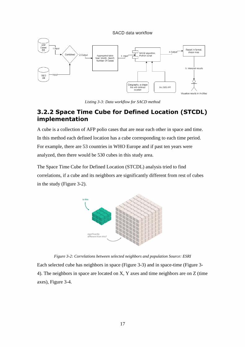
The data workflows of this algorithm were presented in Listing 3.3. In summary, the

data was aggregated. (Listing 3.3 step 1 and 2). Then, the python application (Listing

3.3 step 3) used Arc GIS API to execute the SACD analysis. It outputs results into an

Arc GIS shape file format, that can easily be visualized and modified (Listing 3.3 step

4 and 5).

17

Listing 3-3: Data workflow for SACD method

3.2.2 Space Time Cube for Defined Location (STCDL)

implementation

A cube is a collection of AFP polio cases that are near each other in space and time.

In this method each defined location has a cube corresponding to each time period.

For example, there are 53 countries in WHO Europe and if past ten years were

analyzed, then there would be 530 cubes in this study area.

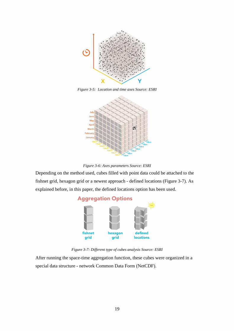
The Space Time Cube for Defined Location (STCDL) analysis tried to find

correlations, if a cube and its neighbors are significantly different from rest of cubes

in the study (Figure 3-2).

Figure 3-2: Correlations between selected neighbors and population Source: ESRI

Each selected cube has neighbors in space (Figure 3-3) and in space-time (Figure 3-

4). The neighbors in space are located on X, Y axes and time neighbors are on Z (time

axes), Figure 3-4.

18

Figure 3-3: A cube (purple) with its neighbors in space Source: ESRI

Figure 3-4: A cube (purple) with its neighbors in space and time Source: ESRI

In other words, the points (AFP cases) have been aggregated in cubes (Figure 3-5).

The points were gathered in cubes (bins, in other literature) that were near each other

in time and space, X corresponding to longitude and respectively Y- to latitude. For

easy visualization the time and distance parameters were shown on the cube axis in

Figure 3-6.

A new method was introduced in the software ArcGIS Pro, called Space Time Cube

for Defined Locations (STCDL), because it met WHO requirements. It used Mann-

Kendall statistics that took into account administrative borders, along with past

information to produce a spatial analysis for potential outbreak prevention. In

addition, it calculated the Getis-Ord Gi statistics for the hot spot analysis. The

resultant z-scores and p-values tell you where there were features with either high or

low values cluster spatially10.

10 How Hot Spot Analysis (Getis-Ord Gi) works; http://pro.arcgis.com/en/pro-app/tool-

reference/spatial-statistics/h-how-hot-spot-analysis-getis-ord-gi-spatial-stati.htm

19

Figure 3-5: Location and time axes Source: ESRI

Figure 3-6: Axes parameters Source: ESRI

Depending on the method used, cubes filled with point data could be attached to the

fishnet grid, hexagon grid or a newest approach - defined locations (Figure 3-7). As

explained before, in this paper, the defined locations option has been used.

Figure 3-7: Different type of cubes analysis Source: ESRI

After running the space-time aggregation function, these cubes were organized in a

special data structure - network Common Data Form (NetCDF).

20

NetCDF is a self-describing, machine-independent data format that supports the

creation, access, and sharing of array-oriented scientific data11.

Furthermore, during the cubes initialization the time trend is calculated. It relies on

Mann-Kendall statistics12. It is a non-parametric test for identifying trends in times

series. One benefit of it is that data does not require confirmation to any particular

distribution shape.

The Mann-Kendall trend test was performed on every location with data as an

independent cube time-step test. The Mann-Kendall statistic is a rank correlation

analysis for the cube count or value and their time intervals13. The cube value for the

first time period was compared to the cube value for the second. If the first was

smaller than the second, the result was a +1. If the first was larger than the second, the

result was -1. If the two values were tied, the result was zero. The results for each pair

of time periods compared were summed. When expected sum was zero, indicating no

trend in the values over time. Based on the variance for the values in the cube time

series, the number of ties, and the number of time periods, the observed sum was

compared to the expected sum (zero) to determine if the difference was statistically

significant or not.

The trend for each cube time series was recorded as a z-score and a p-value. A small

p-value indicates the trend was statistically significant. The sign associated with the z-

score determines if the trend was an increase in cube values (positive z-score) or a

decreased in cube values (negative z-score)11.

Formally, the initial value of the Mann-Kendall statistic S, was assumed to be 0 (no

trend). If a data value from a later time period was higher than a data value from an

earlier time period, S was incremented by 1. On the other hand, if the data value from

a later time period was lower than a data value sampled earlier, S would be

decremented by 1. The net result of all such increments and decrements yields the

final value of S11.

11 NetCDF Fact Sheet;

https://www.unidata.ucar.edu/publications/factsheets/current/factsheet_netcdf.pdf 12 Khambhammettu Prashanth; Mann-Kendall statistics memorandum;

http://www.statisticshowto.com/wp-content/uploads/2016/08/Mann-Kendall-Analysis-1.pdf 13 “How Creating a Space Time Cube works”; http://pro.arcgis.com/en/pro-app/tool-reference/space-

time-pattern-mining/learnmorecreatecube.htm

21

Let x1, x2, … xn represent n data points where xj represents the data point at time j.

The Mann-Kendall Statistics (S) is as following:

𝑆 = ∑ ∑ 𝑠𝑖𝑔𝑛(𝑥𝑗 − 𝑥𝑘)

𝑛

𝑗=𝑘+1

𝑛−1

𝑘=0

𝑠𝑖𝑔𝑛(𝑥𝑗 − 𝑥𝑘) {

1, 𝑥𝑗 − 𝑥𝑘 > 0

0, 𝑥𝑗 − 𝑥𝑘 = 0

−1, 𝑥𝑗 − 𝑥𝑘 < 0

A very high positive value of S is an indicator of an increasing trend, and a very low

negative value indicates a decreasing trend. However, it is necessary to compute the

probability associated with S and the sample size n.

𝑉𝐴𝑅(𝑆) = 1

18[𝑛(𝑛 − 1)(2𝑛 + 5) − ∑𝑡𝑝(𝑡𝑝 − 1)(2𝑡𝑝 + 5)

𝑔

𝑝=𝑡

]

Where n is the number of data points, g is the number of tied groups (a tied group is a

set of sample data having the same value), and tp is the number of data points in the

pth group14.

A normalized test statistics Z could be computed as follows 13:

{

𝑆 > 0, 𝑍 =

𝑆 − 1

[𝑉𝐴𝑅(𝑆)]1/2

𝑆 = 0, 𝑍 = 0

𝑆 < 0, 𝑍 = 𝑆 + 1

[𝑉𝐴𝑅(𝑆)]1/2

Visually, when STCDL analysis have been executed, it iterated each cube, found the

space-time neighbors (Figure 3-8) and calculated the significance of the cube. An

example result is show in Figure 3-9.

14 Khambhammettu Prashanth; Mann-Kendall statistics memorandum; Page 20

22

Figure 3-8: Example of one cube iteration Source: ESRI

Figure 3-9: Example of results with all classified cubes Source: ESRI

Finally, the hot spot analysis technique, classified the space-time cubes into a

summary layer, shown in figure 3-10. There are 12 categories (Figure 3-10) in the

classification from “new hot spot” to “no trend detected”. An example of space-time

analysis (yellow circle in figure 3-10) classified as “sporadic hot spot” because, over

time it was changing state from cold and hot spots and in last cube, it was a new hot

spot.

Also, for identification of hot spots the Getis-Ord local statistics was used. As a

prerequisite for the calculation of Getis-Ord local let’s consider that:

xj is the attribute value for feature j

wi,j is the spatial weight between feature i and j

23

n is the total number of the features.

�̅� =∑ 𝑥𝑗𝑛𝑗=1

𝑛

𝑆 = √∑ 𝑥𝑗

2𝑛𝑗=1

𝑛− (�̅�)2

The Getis-Ord local is calculated as following:

𝐺𝑖 =∑ 𝑤𝑖,𝑗𝑥𝑗 − �̅� ∑ 𝑤𝑖,𝑗

𝑛𝑗=1

𝑛𝑗=1

𝑆√[𝑛∑ 𝑤𝑖,𝑗

2𝑛𝑗=1 − (∑ 𝑤𝑖,𝑗

𝑛𝑗=1 )

2]

𝑛 − 1

The Gi for each feature in the dataset is a z-score. For statistically significant positive

z-scores, the larger the z-score is, the more intense the clustering of high values or hot

spot. For statistically significant negative z-scores, the smaller the z-score is, the more

intense the clustering of low values or cold spot15.

Figure 3-10: Final results classification Source: ESRI

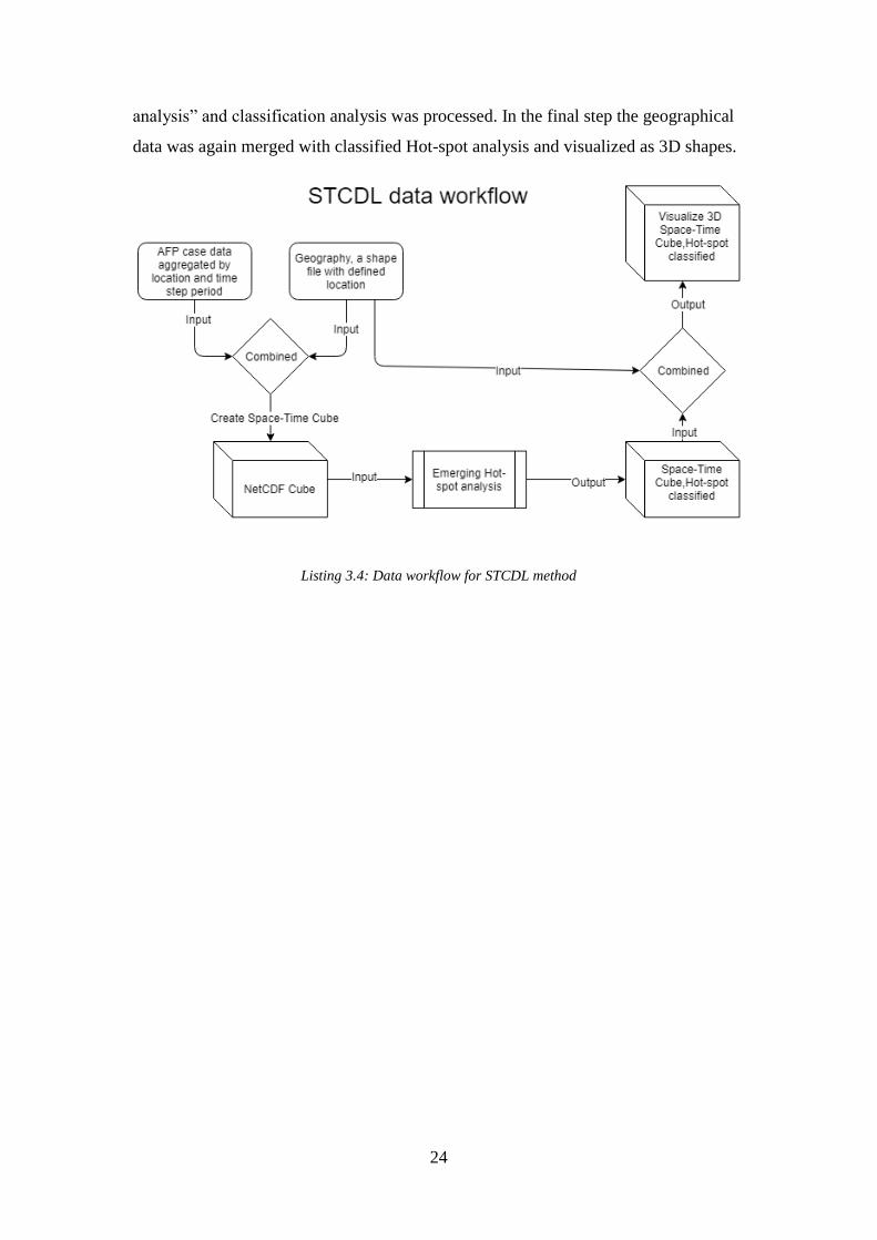
A data workflow for STCDL analysis was showed in listing 3.4. In summary, the

aggregated by location AFP cases were combined with geographical locations

features the NetCDF cubes structure was created. Then a “Emergency Hot-spot

15 How Hot Spot Analysis (Getis-Ord Gi) works; page 18

24

analysis” and classification analysis was processed. In the final step the geographical

data was again merged with classified Hot-spot analysis and visualized as 3D shapes.

Listing 3.4: Data workflow for STCDL method

25

4 RESULTS

4.1 Case study Nigeria

4.1.1 Analysis of AFP cases, SACD results

Maps displayed in figure 4-1 and 4-2 show the districts highlighted using the SACD

algorithm. It presented how polio disease has evolved over a five years period in

Nigeria. In the first series of maps (Figure 4-1), a cluster sensitivity parameter of 30

was used.

Figure 4.1: Nigeria, spatial-temporal analysis, cluster sensitivity parameter: 30

These highlighted territories were indeed low performing districts and suffered with

multiple polio outbreaks in the past. In addition, the data was validated from the graph

in figure 4-3. It shows that the number of cases has consistently increased since 2010

(5988 AFP cases) and peaked in 2016 (17865 AFP cases). It had dropped by 3747

cases in 2017. Considering that the input data for the year 2017 was only partially

available and including up to September 2017, this was an expected behavior.

26

Furthermore, to analyse the clusters of cases, the sensitivity parameter was increased

to 100 and derived a second series of maps (Figure 4-2). All clustered districts (Figure

4-2) were included also in the previous series of maps (Figure 4-1). These districts

had an increase of more than 100 times compared to the previous two years. As a

result, the clusters of high cases became even more evident.

Figure 4.2: Nigeria, spatial-temporal analysis, cluster sensitivity parameter: 100

27

Figure 4.3: Nigeria, distribution of total AFP cases by years

4.1.2 Analysis of AFP cases, STCDL results

As explained in the methods chapter, the first part in the STCDL analysis involved

creating a space time cube (NetCDF structure) for defined locations. In addition, the

STCDL analysis imposed a requirement of a minimum 10 time steps. To solve this

issue, six months steps instead of yearly were chosen, which resulted in ten cubes per

location (ten time steps). The analysis still covers five years.

The mean was used as a parameter for case aggregation. The neighbors in space and

time were used to predict districts that could not be estimated from input data.

This analysis consists of all population AFP cases in Nigeria and is not a fraction

sample. These means that the statistics represent facts for the population and not a

prediction. The overall Mann-Kendall data trend for the analyzed variables was

increasing with a p-value equal to 0,0042 and trend statistics of 2,8622. A low p-value

means that there is a significant trend. The full STCDL summary information was

displayed in appendix, Figure A-1.

The results of hot spot analysis were presented in Figure 4-4.

28

Figure 4-4: Nigeria, AFP Hot Spot analysis

All territories (Figure 4-4) were classified into the following three categories:

consecutive hot spot, oscillating hot spot, areas where no pattern was detected

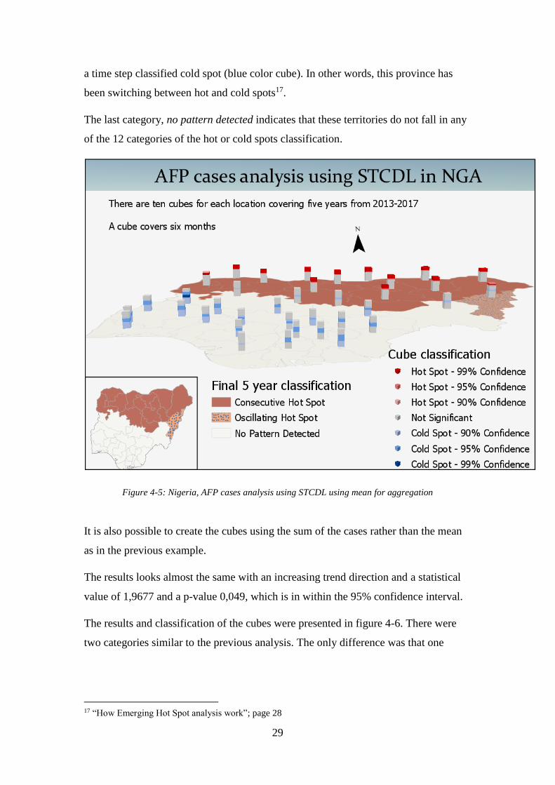
It is clearly visible from figure 4-5 that many territories in the North of Nigeria were

classified as a consecutive hot spot, because they had a high number of cases in final

time-steps (note top cubes colored in red figure 4-5).In other words, a consecutive

hot spot was defined as a single uninterrupted run of statistically significant cubes in

the final time-step intervals (in this study final steps were in 2016,2017 years). Also,

these locations have not been statistically significant hot spot prior to the final hot

spot year and less than ninety percent of all cubes are statistically significant hot

spots16.

In the figure 4-5, one province on the North-East side was classified as oscillating

hot spot because like the previous category “consecutive hot spot” the last cubes were

statistically significant hot spots for the final time-step interval and in addition, it had

16 “How Emerging Hot Spot analysis work”; http://desktop.arcgis.com/en/arcmap/10.3/tools/space-

time-pattern-mining-toolbox/learnmoreemerging.htm

29

a time step classified cold spot (blue color cube). In other words, this province has

been switching between hot and cold spots17.

The last category, no pattern detected indicates that these territories do not fall in any

of the 12 categories of the hot or cold spots classification.

Figure 4-5: Nigeria, AFP cases analysis using STCDL using mean for aggregation

It is also possible to create the cubes using the sum of the cases rather than the mean

as in the previous example.

The results looks almost the same with an increasing trend direction and a statistical

value of 1,9677 and a p-value 0,049, which is in within the 95% confidence interval.

The results and classification of the cubes were presented in figure 4-6. There were

two categories similar to the previous analysis. The only difference was that one

17 “How Emerging Hot Spot analysis work”; page 28

30

location that was previously classified as an oscillating hot-spot, was classified as

having no pattern in this analysis.

Appendix figure A-2 showed the detailed summary table for the cubes creation.

Figure 4-6: Nigeria, AFP cases analysis using STCDL using sums for aggregation

4.1.3 Analysis of zero dose cases, SACD results

An essential and interesting analysis was to detect the location of cases with zero

doses. This was a very important analysis, as every child counts especially in a polio-

endemic country like Nigeria.

The number of cases with zero doses were presented in the figure 4-7. We detected a

sharp decline from 231 in 2010 to 47 in 2016 and 51 in 2017. This decrease was a

consequence of many SIA activities in the country.

31

Figure 4-7: Nigeria, distribution of zero dose AFP cases by years

The algorithm was run with zero dose cases as input. These results were presented in

figure 4-8, 4-9 and 4-10. The sensitivity parameter was important to be

accommodated to amount of input data. In this scenario, only a small fraction (total of

926 zero dose cases) were used from total of 64 000 cases used in the previous

analysis, therefore the sensitivity parameters were much smaller. They were set to 2, 3

and 5 in figure 4-8, 4-9 and 4-10 respectively.

One important aspect of the SACD algorithm, is that cluster of cases in a defined

location could be significant only if it exceeds the total of reported cases in same

period of past year multiplied by cluster sensitivity parameter. In other words, a

cluster parameter of 2 means twice as big compared to previous year or 100 means

one hundred times as big compared to previous year.

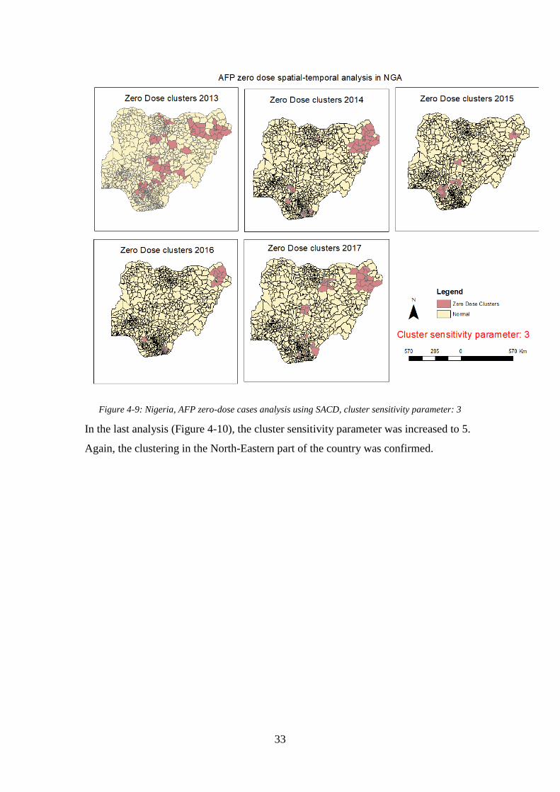
In the maps shown in figure 4-8, there was a gradual decrease in the number of

selected districts from 2013 to 2016. These districts had twice the number of zero

dose cases compared to the previous two years. These allowed us to make a

conclusion, that the most vulnerable districts were located in the North-East part of

Nigeria.

32

Figure 4-8: Nigeria, AFP zero-dose cases analysis using SACD, cluster sensitivity parameter: 2

In figure 4-9, the cluster sensitivity parameter was slightly increased from 2 to 3. It

was now more illustrative that a cluster in North-East of the country was more

distinct.

33

Figure 4-9: Nigeria, AFP zero-dose cases analysis using SACD, cluster sensitivity parameter: 3

In the last analysis (Figure 4-10), the cluster sensitivity parameter was increased to 5.

Again, the clustering in the North-Eastern part of the country was confirmed.

34

Figure 4-10: Nigeria, AFP zero-dose cases analysis using SACD, cluster sensitivity parameter: 5

4.1.4 Analysis of zero dose cases, STCDL results

The NetCDF structure for STCDL of zero dose cases analysis has been created. As in

a previous analysis, the six months steps were used for last five years, resulting in ten

cubes per location. The Mann-Kendall trend statistics resulted in a insignificant trend.

The p-value is 0.5296 and the trend statistics is -0.5410. It would have been a

negative trend, but since the p-value was so high, the trend has been classified as

insignificant. The full summary information was presented in figure A-3.

The final hot spot analysis classification and cubes were presented in figure 4-11.

For most of the area, there was no pattern detected, but for the North-East part of the

country a “Sporadic Hot Spot” was detected. This coming and going hot spot

behavior was visible in cubes from the North-East part of the country

In other words, it was classified as a location that was an on-again then off-again hot

spot. Less than ninety percent of the time-step intervals have been statistically

35

significant hot spots and none of the time-step intervals have been statistically

significant cold spots18. It was interesting to notice a similar behavior in the North-

East part in the map from the SACD algorithm presented earlier.

Figure 4-11: Nigeria, AFP Zero cases analysis using STCDL, using sum for aggregation

4.2 Case study WHO Europe

4.2.1 Analysis of AFP cases, SACD results

The WHO European region had the last indigenous case of poliomyelitis in 1998 and

was certified as polio free by the European Regional Certification Commission for

Poliomyelitis Eradication (RCC) in 2002 (Khetsuriani et. al 2014).

Nevertheless, it had fewer AFP cases compared to Nigeria and therefore, the

parameters for cluster sensitivity were lower. The SACD analysis results were

displayed in figure 4-12 and 4-13. The cluster sensitivity parameter was set to 40 and

respectively 50. The data for the past 10 years (2007- 2017) was analyzed, but since

the SACD requires data for minimum past two years the first report started in 2009.

18 “How Emerging Hot Spot analysis work”; page 28

36

An important cluster of cases in the South-East part of the region has been detected in

2010. This is significant because, a large-scale outbreak occured in 2010. It had

started in Tajikistan caused by the introduction of WPV1 of Indian origin

(Khetsuriani et. al 2014) and spread to neighboring countries: Russian Federation,

Turkmenistan and Kazakhstan. In the presented results, Turkmenistan and Kyrgyzstan

did report a large number of AFP cases in 2010.

Luckily, after large scale SIA activities, the virus transmission was stopped in the

same year and WHO Europe kept its polio free status. Please note that, Tajikistan

continued to report a large number of AFP cases in the following years 2011-2013

(Figure 4-12).

In addition is worth mentioning that there was a significant cluster of AFP cases in

Israel in 2013. Both cluster sensitivity parameters of 40 and 50 have detected the

trend. It was caused by an importation of WPV1 into the Gaza Strip and West Bank.

WPV1 of Pakistani origin was detected in sewage samples. No cases of paralytic

polio were reported (Khetsuriani et. al 2014).

There were clusters detected in the south of the WHO European region: Bulgaria and

the Republic of Macedonia in 2009 and Serbia in 2013. According to risk analysis,

these countries were classified as low risk (Khetsuriani et. al 2014) and no major

outbreaks have been reported from these countries. There were no patterns detected in

years 2014-2017.

37

Figure 4-12: WHO Europe, spatial-temporal analysis, cluster sensitivity parameter: 40

Figure 4-13: WHO Europe, spatial-temporal analysis, cluster sensitivity parameter: 50

38

4.2.2 Analysis of AFP cases, STCDL results

The analysis covered data for 2017-2018 which resulted in 12 steps; each year is one

step. The STCDL requires a minimum of 10 steps. The resulting summary table was

presented in Figure A-4. The Mann-Kendall trend statistics is not significant a with p-

value of 0,3037 (higher then 95% confidence interval) and trend statistics of 1,0286.

Neighbors in space and time were used to fill the empty cubes, but still during the

creation of the NetCDF structure 26 out of 54 defined locations were excluded from

STCDL due to the presence of cubes that could not be estimated. A minimum of 4

neighbors are required to fill empty cubes using the average value of spatial

neighbors, and a minimum of 13 neighbors are required to fill empty cubes using the

average value of space time neighbors19 .

The final map with hot spot cubes is shown in figure 4-14. Even though the trend is

insignificant, the outbreak in the region was depicted by three countries Tajikistan,

Kyrgyzstan and Russian Federation.

The STCDL analysis did show an issue in the Russian Federation. There was a spread

of polio virus outbreak during 2010, but it was incorrect to show that it happened for

such a long period. The overall trend is not significant and it was considered an error.

19 “How Creating a Space Time Cube works”; page 20

39

Figure 4-14: WHO Europe, AFP cases analysis using STCDL using sum for aggregation

4.2.3 Analysis of zero dose cases, SACD results

The result of the SACD analysis of the WHO European region for zero dose cases

was presented in figure 4-15. A cluster parameter of five was used since the amount

of AFP zero dose cases is significantly lower compared to the previous AFP cases

analysis.

The map shows a significant clustering of AFP zero doses in Eastern part of Europe

for all years. According to WHO/UNICEF estimates: Romania and Ukraine are

countries with low polio (Pol3) vaccination coverage and considered high risk

countries for polio outbreak (Khetsuriani et. al 2014).

Also, Israel had been shown with high clustering of AFP zero doses. According to

WHO/UNICEF report it had low vaccination coverage in the past (Khetsuriani et. al

2014).

40

Figure 4-15: WHO Europe, AFP zero-dose cases analysis using SACD, cluster sensitivity parameter: 5

4.2.4 Analysis of zero dose cases, STCDL result

As in previous report STCDL report, the 12 year period was used to perform the

analysis. The Mann-Kendall trend statistics is increasing and significant with a p-

value of 0,0269 and a trend statistics of 2,2135. During the execution of the analysis

49 out of 54 defined locations were removed from the analysis due to cubes that could

not be estimated. The STCDL summary table was presented in figure A-5.

The STCDL result was shown in figure 4-16. Although all remaining countries in the

analysis possess insignificant cubes, still few countries did possess an interest.

Ukraine, Romania and Israel were among the countries that were found with zero

doses AFP clustering. As mentioned by Khetsuriani, these countries are among those

with low polio vaccination coverage.

41

Figure 4-16: WHO Europe, AFP Zero cases analysis using STCDL, using sum for aggregation

42

43

5 DISCUSSION

5.1 Comparison between SACD and STCDL

This research has utilized two approaches to analyze previously reported information

and has identified unusual clustering of diseases in space and time. First, an algorithm

called SACD was developed specifically for this assignment to isolate those areas

related to polio. Secondly, scientifically proven Mann-Kendall and Getis-Ord Gi

methods, described in STCDL algorithm have been chosen to find patterns in two

study areas: Nigeria and WHO Europe.

The SACD algorithm was controlled by a sensitivity cluster parameter, which was

dependent on the amount of input data. For Nigeria with more than 64 000 AFP cases

reported in the past five years, cluster parameters of 30 and 100 were used. For WHO

Europe with more than 19 000 AFP cases reported within the past 12 years, it was

used cluster parameters of 40 and 50. In addition, a fraction of reported cases were

utilized in the analysis of circumstances involving of non-vaccinated (Zero doses)

children. Kindly note, that monitoring these cases are important factors for polio

eradication. For this situation where total AFP zero doses correspond to 926 cases in

Nigeria a much lower cluster sensitivity parameter was used, respectively: 2, 3 and 5.

Although there was a correlation between the size the of data and cluster sensitivity,

in SACD, there was no direct guidance on how the cluster sensitivity parameter was

decided. Instead, a trial of many parameters were used to detect these clustered

territories. In contrast, STCDL algorithm relied on statistical models, which provided

scientifically proven results based on probabilistic statistical methods.

STCDL has a disadvantage that it requires a high amount of input. In addition, it

needs at least ten times the number of period steps and each location must have a

value at every time step. There must be a decision on how to complete the time series

using the method of filling empty cubes with a value taken from their neighbors in

space and time. The SACD algorithm does not require a complete time series, but it

removes those locations that have empty values (No AFP cases were reported).

SACD and STCDL analyses were almost identical in nature because they were using

similar input data and generated reports for the same defined geographical location.

Also, the results yielded cluster in close semblance. For example, in Nigeria there was

44

an issue in the North-Eastern part of the country (Inwa Barau et. al 2014). Both

algorithms have detected these outbreaks in zero dose cases analysis. There was a

significant difference between results of these two algorithms in analysis of the total

number of cases. STCDL showed a clear issue in Northern Nigeria (Figure 4-5) and

the SACD were distributed across Nigeria.

Finally, the major multi-national outbreak of polio in 2010 in Tajikistan (Khetsuriani

et. al 2014) and one in Israel 2013 (Khetsuriani et. al 2014) were detected and

visualized by both SACD and STCDL.

To keep the STCDL analysis manageable it was decided to aggregate them with 37

provinces at the first administrative level. However, visualizing the cubes consumed a

large portion of GPU and memory. Conducting the STCDL analysis using more than

100 locations would become very difficult for on one computer. To visualize 37

provinces, required removing hardware limits and waiting approximately five

minutes. In contrast, the prototype used to collapse data at the district level, which

consists of more than 700 locations for Nigeria and on same computer the results

were generated in around two minutes. Thus, SACD is executed faster with the same

computer resources.

Another difference between the analyses was how temporary aggregation has been

performed. When creating an STCDL cube from defined locations with temporal

aggregation a summary field statistics has to be chosen. There were several options

for summary: sum, mean, min, max, standard deviation within the cube and median20.

The goal was to find a significant difference in all territories (not only the minimum

or maximum) and mean was utilized in the SACD algorithm from beginning, as well

as in STCDL.

5.2 Integration of analyses into an outbreak

prevention system

Finally a very important aspect of this research was to investigate how to automatize

the process of creating the SACD and STCDL reports into a Standard Operational

Procedure (SOP). The aim was to organize them into an outbreak prevention system

that would cover many countries and territories. Each country has different

20 “How Creating a Space Time Cube works”, page 20

45

requirements and possibilities for data reporting. For example, in a situation of a

disease outbreak an AFP case base surveillance would be insufficient, and an

aggregate reporting system would be optimal to save time. The geographical

information and time are very important for epidemiologists to investigate an

outbreak.

At the regional level WHO Europe, (Vaccine-preventable Diseases and Immunization

Programme of WHO Europe) VPI was using (Centralized Information System for

Infectious Diseases) CISID and (Laboratory Data Management System) LDMS to

collect AFP cases and laboratory sample data (Figure A-5). These systems have been

provided to member states both aggregated (in case of outbreak) and case based

reporting capabilities.

A key functionality designed by VPI and implemented in LDMS was “weekly AFP

temporal clustering alerts”. It was a program that ran automatically on a weekly basis.

The algorithm verified each country and when a reported AFP cases did exceed a

threshold of cumulative cases reported in the past year then it would generate a table

report with countries and the total number of hot cases (Figure A-5). In addition, it

has implemented some restrictions for “hot” AFP cases.

Finally, the algorithm will detect if there are potential hot cases and then output would

be sent by email to the focal point (epidemiologist). The analysis developed here

could be integrated with cluster maps of cases and help with early warning.

The main issue addressed in this paper was to utilize the borders between existing

countries to analyze reported AFP cases and generate reports for potential clustering.

More specifically, the developed analysis could be integrated into an automatic SOP

for the creation of routine reports and potential outreach, thus informing focal points

of such unusual situations (Listing 4-1). SACD algorithm program was modularized

so it could be easily integrated into the LDMS “hot” AFP case algorithm and

routinely used by health specialists (Listing 4-1).

46

Listing 4-1: Outbreak prevention system data workflow

In summary, the health specialists from members states fill-in the forms with AFP

cases (Listing 4-1 step 1) on a weekly basis in the CISID. Then a map report analysis

is generated each week (Listing 4-1 step 2). When a report contains clusters of hot

AFP cases, then it would be sent by email for a review to a VPI epidemiologist

(Listing 4-1 step 4 and 5). He would be responsible for verifying the accuracy,

creating the final version of the report and disseminating the results among member

states, and publishing it on the website (Listing 4-1 step 6 and 7). Automatic reports

like STCDL, and SACD should not be published directly, but their results should be

verified and clarified before they are disseminated.

47

6 CONCLUSIONS

In order to fulfill the requirements for this paper an experimental prototype

application has been developed that implemented SACD algorithm. Fortunately,

during the data research it was found that Arc GIS Pro, which is a new product from

ESRI, supports a similar method for analysis that meets the needs for this study. This

was not possible to do in ArcMap, and therefore for this paper a license for ArcGIS

Pro was offered by WHO. This made possible for this work to use both SACD

prototype and STCDL implementation. These techniques were used to explore spatio-

temporal clustering for two case studies: Nigeria and the WHO European region.

Furthermore, with regards to the first objective, this prototype (SACD algorithm) was

designed to determine defined location with significant clustering of cases. Using the

supplied dataset of AFP cases the analysis has been executed successfully.

In comparison to STCDL that relies on probabilistic determinants, the SACD does

consider using of a sensitivity cluster parameter. Although there was a direct

correlation between the input data and cluster sensitivity, still number of tests were

carried out to determine the optimal parameter for cluster sensitivity. As a rule of

thumb, a low parameter is tested first, then gradually increased until an optimal

picture with defined location clusters was obtained. Both newly developed model

SACD and validation model STCDL have demonstrated a significant clustering issue

of AFP cases in the northen part of Nigeria.

One of the more significant findings to emerge from this study was from spatio-

temporal analyses in WHO Europe. As of result a new innovative SACD the multi-

national polio outbreak in 2010 (Khetsuriani et. al 2014) have been spotted. It started

in Tajikistan and spread to neighboring countries. It was followed by a massive SIA

vaccination for children and the polio outbreak stopped in the same year (Khetsuriani

et. al 2014). Another major finding by SACD, was identified in Israel, another polio

outbreak detected in 2013 in the WHO European region (Khetsuriani et. al 2014).

Also, the validation model STCDL was in most part consistent with SACD.

The second objective, of this paper was to evaluate the vulnerable unvaccinated

children. In this investigation, the aim was to assess AFP cases with zero dose

vaccinations which is a small fraction of total AFP cases reported. As the input data

48

was considerably less than in previous analyses, the cluster sensitivity parameters

were respectively lower. Nevertheless, the SACD and STCDL have identified an

issue in the North-East of Nigeria. In addition, the South-East part of Europe

identified a significant cluster. Romania and Ukraine were considered particularly

high risk countries because of low polio vaccination coverage (Khetsuriani et. al

2014).

The evidence from this study suggests that there is no active outbreak in WHO

Europe in the past year, but there were still major issues in Nigeria. These analyses

could have a practical application in routinely usage, if incorporated in an outbreak

prevention system. It would analyze the reported data on a defined time period (for

example weekly). If something unusual was detected then health specialists would be

informed so they could take further prevention actions.

49

References

Abatan A. Abayomi, Babatunde J. Abiodun, William J. Gutowski, Saidat O. Rasaq-

Balogun; Trends and variability in absolute indices of temperature extremes

over Nigeria: linkage with NAO; 2017; Royal Meteorological Society;

International Journal of Climatology; vol 38; no. 2; pp. 593-612

Elliott Paul and Daniel Wartenberg; Spatial Epidemiology: Current Approaches and

Future Challenges; 2004; Environmental Health Perspective; vol. 112; no.9; pp.

998–1006

Ibrahim Sa’ad,Isah Hamisu, Usman Lawal; Spatial Pattern of Tuberculosis

Prevalence in Nigeria: A Comparative Analysis of Spatial Autocorrelation

Indices; 2015; American Journal of Geographic Information System; vol. 2; no.

3; pp 87-94

Khetsuriani Nino, Dina Pfeifer, Sergei Deshevoi, Eugene Gavrilin, Abigail Shefer,

Robb Butler, Dragan Jankovic, Roman Spataru, Nedret Emiroglu, and Rebecca

Martin. Challenges of Maintaining Polio-free Status of the European Region;

2014; The Journal of Infectious Disease; Oxford University Press; vol. 210; no.

1; pp. S194-S207;

Mahara Gehendra, Chao Wang, Da Huo, Qin Xu, Fangfang Huang, Lixin Tao, Jin

Guo, Kai Cao, Liu Long, Jagadish K. Chhetri, Qi Gao, Wei Wang, Quanyi

Wang and Xiuhua Guo; Spatiotemporal Pattern Analysis of Scarlet Fever

Incidence in Beijing, China, 2005–2014; 2016; International Journal

Environmental Research and Public Health; vol. 13; no. 131; pp. 2-17

Rogerson Peter A.; Statistical Methods for Geography; 2015; Fourth Edition; SAGE

Publications; ISBN 9780761962878;

Tango Toshiro; Statistical Methods for Disease Clustering; 2010; Springer New

York, ISBN: 9781441915726;

Tlou Boikhutso, Benn Sartorius1, Frank Tanser1; Space-time variations in child

mortality in a rural South African population with high HIV prevalence (2000–

2014); 2017; A Peer-Reviewed Open Access Journal (PLoS One); vol. 12; no.

8; pp. 1-13

50

Toshiro Tango, Kunihiko Takahashi; A flexibly shaped spatial scan statistic for

detecting clusters; 2005; 10.1186/1476-072X-4-11; International Journal of

Health Geographics; vol. 4; no. 1; pp. 1-15

Uittenbogaard Adriaan and Vania Ceccato; Space-time Clusters of Crime in

Stockholm, Sweden; 2012; Review of European Studies; Published by Canadian

Center of Science and Education; vol. 4; no. 5; pp. 148-156

Zhao Fei, Shiming Cheng1, Guangxue He1, Fei Huang1, Hui Zhang1, Biao Xu,

Tonderayi C. Murimwa, Jun Cheng1, Dongmei Hu1, Lixia Wang1; Space-Time

Clustering Characteristics of Tuberculosis in China, 2005-2011; 2013; A Peer-

Reviewed Open Access Journal (PLoS One); vol. 8; no. 12; pp. 1-7

51

Appendix A

Figure A-1:Nigeria, AFP cases, space-time cube summary, using MEAN for aggregation

52

Figure A-2: Nigeria, AFP cases, space-time cube summary, using SUM for aggregation

53

Figure A-3: Nigeria, zero dose AFP cases, space-time cube summary, using SUM for aggregation

54

Figure A-4: WHO Europe, AFP cases, space-time cube summary, using SUM for aggregation

55

Figure A-5: WHO Europe, zero dose AFP cases, space-time cube summary, using SUM for

aggregation

56

Figure A-6: Online LDMS and CISID workflow

57

Appendix B

ESRI, Environmental Systems Research Institute; An overview of the Spatial Statistics

toolbox; [Online] Available at: http://pro.arcgis.com/en/pro-app/tool-

reference/spatial-statistics/an-overview-of-the-spatial-statistics-toolbox.htm

[Accessed 17 March 2018]

ESRI; How Creating a Space Time Cube works; [Online] Available at:

http://pro.arcgis.com/en/pro-app/tool-reference/space-time-pattern-

mining/learnmorecreatecube.htm [Accessed 17 March 2018]

ESRI; How Emerging Hot Spot analysis work; [Online] Available at:

http://desktop.arcgis.com/en/arcmap/10.3/tools/space-time-pattern-mining-

toolbox/learnmoreemerging.htm [Accessed 17 March 2018]

ESRI; How Hot Spot Analysis (Getis-Ord Gi) works; [Online] Available at:

http://pro.arcgis.com/en/pro-app/tool-reference/spatial-statistics/h-how-hot-

spot-analysis-getis-ord-gi-spatial-stati.htm [Accessed 17 March 2018]

ESRI; Spatial Statistics; [Online] Available at:

https://spatialstats.github.io/presentations/ [Accessed 17 March 2018]

Khambhammettu Prashanth; Mann-Kendall statistics memorandum; 2005; Annual

Groundwater Monitoring Report; [Online] Available at:

http://www.statisticshowto.com/wp-content/uploads/2016/08/Mann-Kendall-

Analysis-1.pdf [Accessed 17 March 2018]

Lixin Huang; Analyzing traffic accidents in space and time; [Online] Available at:

http://desktop.arcgis.com/en/analytics/case-studies/analyzing-crashes-1-

overview.htm [Accessed 17 March 2018]

Unidata’s Network Common Data Form; NetCDF Fact Sheet; [Online] Available at:

https://www.unidata.ucar.edu/publications/factsheets/current/factsheet_netcdf.p

df [Accessed 17 March 2018]

WHO European Region; Report of the 30th Meeting of the European RCC for

Poliomyelitis Eradication; 2016; [Online] Available at:

http://www.euro.who.int/en/health-topics/communicable-

diseases/poliomyelitis/publications/2016/30th-meeting-of-the-european-

58

regional-certification-commission-for-poliomyelitis-eradication [Accessed 17

March 2018]

WHO; Factsheet Polio Euro; [Online] Available at:

http://www.euro.who.int/__data/assets/pdf_file/0005/276485/Factsheet-Polio-

en.pdf [Accessed 17 March 2018]

WHO; Poliomyelitis, key facts; [Online] Available at: http://www.who.int/news-

room/fact-sheets/detail/poliomyelitis [Accessed 17 March 2018]

WHO; WHO Removes Nigeria from Polio-Endemic List; [Online] Available at:

http://www.who.int/mediacentre/news/releases/2015/nigeria-polio/en/

[Accessed 17 March 2018]

59

Series from Lund University

Department of Physical Geography and Ecosystem Science

Master Thesis in Geographical Information Science

1. Anthony Lawther: The application of GIS-based binary logistic regression for slope failure susceptibility mapping in the Western Grampian Mountains, Scotland (2008).

2. Rickard Hansen: Daily mobility in Grenoble Metropolitan Region, France. Applied GIS methods in time geographical research (2008).

3. Emil Bayramov: Environmental monitoring of bio-restoration activities using GIS and Remote Sensing (2009).

4. Rafael Villarreal Pacheco: Applications of Geographic Information Systems as an analytical and visualization tool for mass real estate valuation: a case study of Fontibon District, Bogota, Columbia (2009).

5. Siri Oestreich Waage: a case study of route solving for oversized transport: The use of GIS functionalities in transport of transformers, as part of maintaining a reliable power infrastructure (2010).

6. Edgar Pimiento: Shallow landslide susceptibility – Modelling and validation (2010).

7. Martina Schäfer: Near real-time mapping of floodwater mosquito breeding sites using aerial photographs (2010).

8. August Pieter van Waarden-Nagel: Land use evaluation to assess the

outcome of the programme of rehabilitation measures for the river Rhine in

the Netherlands (2010).

9. Samira Muhammad: Development and implementation of air quality data

mart for Ontario, Canada: A case study of air quality in Ontario using OLAP

tool. (2010).

10. Fredros Oketch Okumu: Using remotely sensed data to explore spatial and

temporal relationships between photosynthetic productivity of vegetation and

malaria transmission intensities in selected parts of Africa (2011).

11. Svajunas Plunge: Advanced decision support methods for solving diffuse

water pollution problems (2011).

12. Jonathan Higgins: Monitoring urban growth in greater Lagos: A case study

using GIS to monitor the urban growth of Lagos 1990 - 2008 and produce

future growth prospects for the city (2011).

13. Mårten Karlberg: Mobile Map Client API: Design and Implementation for

Android (2011).

14. Jeanette McBride: Mapping Chicago area urban tree canopy using color

infrared imagery (2011).

15. Andrew Farina: Exploring the relationship between land surface temperature

and vegetation abundance for urban heat island mitigation in Seville, Spain

(2011).

16. David Kanyari: Nairobi City Journey Planner: An online and a Mobile

Application (2011).

60

17. Laura V. Drews: Multi-criteria GIS analysis for siting of small wind power

plants - A case study from Berlin (2012).

18. Qaisar Nadeem: Best living neighborhood in the city - A GIS based multi

criteria evaluation of ArRiyadh City (2012).

19. Ahmed Mohamed El Saeid Mustafa: Development of a photo voltaic

building rooftop integration analysis tool for GIS for Dokki District, Cairo,

Egypt (2012).

20. Daniel Patrick Taylor: Eastern Oyster Aquaculture: Estuarine Remediation

via Site Suitability and Spatially Explicit Carrying Capacity Modeling in

Virginia’s Chesapeake Bay (2013).

21. Angeleta Oveta Wilson: A Participatory GIS approach to unearthing

Manchester’s Cultural Heritage ‘gold mine’ (2013).

22. Ola Svensson: Visibility and Tholos Tombs in the Messenian Landscape: A

Comparative Case Study of the Pylian Hinterlands and the Soulima Valley

(2013).

23. Monika Ogden: Land use impact on water quality in two river systems in

South Africa (2013).

24. Stefan Rova: A GIS based approach assessing phosphorus load impact on

Lake Flaten in Salem, Sweden (2013).

25. Yann Buhot: Analysis of the history of landscape changes over a period of

200 years. How can we predict past landscape pattern scenario and the

impact on habitat diversity? (2013).

26. Christina Fotiou: Evaluating habitat suitability and spectral heterogeneity

models to predict weed species presence (2014).

27. Inese Linuza: Accuracy Assessment in Glacier Change Analysis (2014).

28. Agnieszka Griffin: Domestic energy consumption and social living

standards: a GIS analysis within the Greater London Authority area (2014).

29. Brynja Guðmundsdóttir: Detection of potential arable land with remote

sensing and GIS - A Case Study for Kjósarhreppur (2014).

30. Oleksandr Nekrasov: Processing of MODIS Vegetation Indices for analysis

of agricultural droughts in the southern Ukraine between the years 2000-

2012 (2014).

31. Sarah Tressel: Recommendations for a polar Earth science portal

in the context of Arctic Spatial Data Infrastructure (2014).

32. Caroline Gevaert: Combining Hyperspectral UAV and Multispectral

Formosat-2 Imagery for Precision Agriculture Applications (2014).

33. Salem Jamal-Uddeen: Using GeoTools to implement the multi-criteria

evaluation analysis - weighted linear combination model (2014).

34. Samanah Seyedi-Shandiz: Schematic representation of geographical railway

network at the Swedish Transport Administration (2014).

35. Kazi Masel Ullah: Urban Land-use planning using Geographical Information

System and analytical hierarchy process: case study Dhaka City (2014).

36. Alexia Chang-Wailing Spitteler: Development of a web application based on

MCDA and GIS for the decision support of river and floodplain

rehabilitation projects (2014).

37. Alessandro De Martino: Geographic accessibility analysis and evaluation of

potential changes to the public transportation system in the City of Milan

(2014).

38. Alireza Mollasalehi: GIS Based Modelling for Fuel Reduction Using

Controlled Burn in Australia. Case Study: Logan City, QLD (2015).

61

39. Negin A. Sanati: Chronic Kidney Disease Mortality in Costa Rica;

Geographical Distribution, Spatial Analysis and Non-traditional Risk Factors

(2015).

40. Karen McIntyre: Benthic mapping of the Bluefields Bay fish sanctuary,

Jamaica (2015).

41. Kees van Duijvendijk: Feasibility of a low-cost weather sensor network for

agricultural purposes: A preliminary assessment (2015).

42. Sebastian Andersson Hylander: Evaluation of cultural ecosystem services

using GIS (2015).

43. Deborah Bowyer: Measuring Urban Growth, Urban Form and Accessibility

as Indicators of Urban Sprawl in Hamilton, New Zealand (2015).

44. Stefan Arvidsson: Relationship between tree species composition and

phenology extracted from satellite data in Swedish forests (2015).

45. Damián Giménez Cruz: GIS-based optimal localisation of beekeeping in

rural Kenya (2016).

46. Alejandra Narváez Vallejo: Can the introduction of the topographic indices

in LPJ-GUESS improve the spatial representation of environmental

variables? (2016).

47. Anna Lundgren: Development of a method for mapping the highest coastline

in Sweden using breaklines extracted from high resolution digital elevation

models (2016).

48. Oluwatomi Esther Adejoro: Does location also matter? A spatial analysis of

social achievements of young South Australians (2016).

49. Hristo Dobrev Tomov: Automated temporal NDVI analysis over the Middle

East for the period 1982 - 2010 (2016).

50. Vincent Muller: Impact of Security Context on Mobile Clinic Activities

A GIS Multi Criteria Evaluation based on an MSF Humanitarian Mission in

Cameroon (2016).

51. Gezahagn Negash Seboka: Spatial Assessment of NDVI as an Indicator of

Desertification in Ethiopia using Remote Sensing and GIS (2016).

52. Holly Buhler: Evaluation of Interfacility Medical Transport Journey Times

in Southeastern British Columbia. (2016).

53. Lars Ole Grottenberg: Assessing the ability to share spatial data between

emergency management organisations in the High North (2016).

54. Sean Grant: The Right Tree in the Right Place: Using GIS to Maximize the

Net Benefits from Urban Forests (2016).

55. Irshad Jamal: Multi-Criteria GIS Analysis for School Site Selection in

Gorno-Badakhshan Autonomous Oblast, Tajikistan (2016).

56. Fulgencio Sanmartín: Wisdom-volkano: A novel tool based on open GIS

and time-series visualization to analyse and share volcanic data (2016).

57. Nezha Acil: Remote sensing-based monitoring of snow cover dynamics and

its influence on vegetation growth in the Middle Atlas Mountains (2016).

58. Julia Hjalmarsson: A Weighty Issue: Estimation of Fire Size with

Geographically Weighted Logistic Regression (2016).

59. Mathewos Tamiru Amato: Using multi-criteria evaluation and GIS for

chronic food and nutrition insecurity indicators analysis in Ethiopia (2016).

60. Karim Alaa El Din Mohamed Soliman El Attar: Bicycling Suitability in

Downtown, Cairo, Egypt (2016).

62

61. Gilbert Akol Echelai: Asset Management: Integrating GIS as a Decision

Support Tool in Meter Management in National Water and Sewerage

Corporation (2016).

62. Terje Slinning: Analytic comparison of multibeam echo soundings (2016).

63. Gréta Hlín Sveinsdóttir: GIS-based MCDA for decision support: A

framework for wind farm siting in Iceland (2017).

64. Jonas Sjögren: Consequences of a flood in Kristianstad, Sweden: A GIS-

based analysis of impacts on important societal functions (2017).

65. Nadine Raska: 3D geologic subsurface modelling within the Mackenzie

Plain, Northwest Territories, Canada (2017).

66. Panagiotis Symeonidis: Study of spatial and temporal variation of

atmospheric optical parameters and their relation with PM 2.5 concentration

over Europe using GIS technologies (2017).

67. Michaela Bobeck: A GIS-based Multi-Criteria Decision Analysis of Wind

Farm Site Suitability in New South Wales, Australia, from a Sustainable

Development Perspective (2017).

68. Raghdaa Eissa: Developing a GIS Model for the Assessment of Outdoor

Recreational Facilities in New Cities Case Study: Tenth of Ramadan City,

Egypt (2017).

69. Zahra Khais Shahid: Biofuel plantations and isoprene emissions in Svea and

Götaland (2017).

70. Mirza Amir Liaquat Baig: Using geographical information systems in

epidemiology: Mapping and analyzing occurrence of diarrhea in urban -

residential area of Islamabad, Pakistan (2017).

71. Joakim Jörwall: Quantitative model of Present and Future well-being in the

EU-28: A spatial Multi-Criteria Evaluation of socioeconomic and climatic

comfort factors (2017).

72. Elin Haettner: Energy Poverty in the Dublin Region: Modelling Geographies

of Risk (2017).

73. Harry Eriksson: Geochemistry of stream plants and its statistical relations to

soil- and bedrock geology, slope directions and till geochemistry. A GIS-

analysis of small catchments in northern Sweden (2017).

74. Daniel Gardevärn: PPGIS and Public meetings – An evaluation of public

participation methods for urban planning (2017).

75. Kim Friberg: Sensitivity Analysis and Calibration of Multi Energy Balance

Land Surface Model Parameters (2017).

76. Viktor Svanerud: Taking the bus to the park? A study of accessibility to

green areas in Gothenburg through different modes of transport (2017).

77. Lisa-Gaye Greene: Deadly Designs: The Impact of Road Design on Road

Crash Patterns along Jamaica’s North Coast Highway (2017).

78. Katarina Jemec Parker: Spatial and temporal analysis of fecal indicator

bacteria concentrations in beach water in San Diego, California (2017).

79. Angela Kabiru: An Exploratory Study of Middle Stone Age and Later Stone

Age Site Locations in Kenya’s Central Rift Valley Using Landscape

Analysis: A GIS Approach (2017).

80. Kristean Björkmann: Subjective Well-Being and Environment: A GIS-Based

Analysis (2018).

81. Williams Erhunmonmen Ojo: Measuring spatial accessibility to healthcare

for people living with HIV-AIDS in southern Nigeria (2018).

63

82. Daniel Assefa: Developing Data Extraction and Dynamic Data Visualization

(Styling) Modules for Web GIS Risk Assessment System (WGRAS). (2018).

83. Adela Nistora: Inundation scenarios in a changing climate: assessing

potential impacts of sea-level rise on the coast of South-East England (2018).

84. Marc Seliger: Thirsty landscapes - Investigating growing irrigation water

consumption and potential conservation measures within Utah’s largest

master-planned community: Daybreak (2018).

85. Luka Jovičić: Spatial Data Harmonisation in Regional Context in

Accordance with INSPIRE Implementing Rules (2018).

86. Christina Kourdounouli: Analysis of Urban Ecosystem Condition Indicators

for the Large Urban Zones and City Cores in EU (2018).

87. Jeremy Azzopardi: Effect of distance measures and feature representations

on distance-based accessibility measures (2018).

88. Patrick Kabatha: An open source web GIS tool for analysis and visualization

of elephant GPS telemetry data, alongside environmental and anthropogenic

variables (2018).

89. Richard Alphonce Giliba: Effects of Climate Change on Potential

Geographical Distribution of Prunus africana (African cherry) in the

Eastern Arc Mountain Forests of Tanzania (2018).

90. Eiður Kristinn Eiðsson: Transformation and linking of authoritative multi-

scale geodata for the Semantic Web: A case study of Swedish national

building data sets (2018).

91. Niamh Harty: HOP!: a PGIS and citizen science approach to monitoring the

condition of upland paths (2018).

92. José Estuardo Jara Alvear: Solar photovoltaic potential to complement

hydropower in Ecuador: A GIS-based framework of analysis (2018).

93. Brendan O’Neill: Multicriteria Site Suitability for Algal Biofuel Production

Facilities (2018).

94. Roman Spataru: Spatial-temporal GIS analysis in public health – a case

study of polio disease (2018).