Journal of Hydrology 542 (2016) 450–462

Contents lists available at ScienceDirect

Journal of Hydrology

journal homepage: www.elsevier .com/locate / jhydrol

Research papers

Spatial interpolation of river channel topography using the shortesttemporal distance

http://dx.doi.org/10.1016/j.jhydrol.2016.09.0220022-1694/� 2016 The Authors. Published by Elsevier B.V.This is an open access article under the CC BY license (http://creativecommons.org/licenses/by/4.0/).

⇑ Corresponding author.E-mail address: zhangyj1015@hotmail.com (Y. Zhang).

Yanjun Zhang a,⇑, Cuiling Xian a, Huajin Chen b, Michael L. Grieneisen b, Jiaming Liu a, Minghua Zhang b

a State Key Laboratory of Water Resources & Hydropower Engineering Science, Wuhan University, Wuhan, ChinabDepartment of Land, Air and Water Resources, University of California Davis, CA, USA

a r t i c l e i n f o a b s t r a c t

Article history:Received 11 October 2015Received in revised form 16 August 2016Accepted 7 September 2016Available online 14 September 2016This manuscript was handled by Peter K.Kitanidis, Editor-in-Chief, with theassistance of Roseanna M. Neupauer,Associate Editor

Keywords:Shortest temporal distanceModified shortest temporal distanceLocally varying anisotropyRiver channel topographyInterpolation

It is difficult to interpolate river channel topography due to complex anisotropy. As the anisotropy isoften caused by river flow, especially the hydrodynamic and transport mechanisms, it is reasonable toincorporate flow velocity into topography interpolator for decreasing the effect of anisotropy. In thisstudy, two new distance metrics defined as the time taken by water flow to travel between two locationsare developed, and replace the spatial distance metric or Euclidean distance that is currently used tointerpolate topography. One is a shortest temporal distance (STD) metric. The temporal distance (TD)of a path between two nodes is calculated by spatial distance divided by the tangent component of flowvelocity along the path, and the STD is searched using the Dijkstra algorithm in all possible paths betweentwo nodes. The other is a modified shortest temporal distance (MSTD) metric in which both the tangentand normal components of flow velocity were combined. They are used to construct the methods for theinterpolation of river channel topography. The proposed methods are used to generate the topography ofWuhan Section of Changjiang River and compared with Universal Kriging (UK) and Inverse DistanceWeighting (IDW). The results clearly showed that the STD and MSTD based on flow velocity were reliablespatial interpolators. The MSTD, followed by the STD, presents improvement in prediction accuracy rel-ative to both UK and IDW.� 2016 The Authors. Published by Elsevier B.V. This is anopenaccess article under the CCBY license (http://

creativecommons.org/licenses/by/4.0/).

1. Introduction

Topographic data of rivers play an important role in modelingand simulating the flow (Harvey and Bencala, 1993), the transportof sediments and pollutants (Marzadri et al., 2014; Wildhaberet al., 2014), the stream-aquifer interactions (Shope et al., 2012),and the hydrologic response of a basin (Mejia and Reed, 2011).These data are typically obtained by conventional ground-basedsurveys based on transverse profiles, also known as cross-sections, at locations selected to capture salient features of thetopography (Legleiter and Kyriakidis, 2008). The data obtainedare often sparse and discrete, and the interpolation and extrapola-tion must be implemented for satisfying the requirements of mod-eling and simulation. Inverse Distance Weighting (IDW), Spline,Kriging and their derivatives are the most common spatial predic-tion techniques (Merwade, 2009; Schwendel et al., 2012), but thestrong anisotropy that exists in the topography of river channels

makes it difficult to predict the topography using those methods(Legleiter and Kyriakidis, 2008).

For the anisotropy of river channel topography, one possiblesolution is to remove certain trends from the original data.Merwade (2009) presented a method for calculating the trend ofriver bathymetry by transforming the Cartesian coordinates tobody-fitted coordinates based on the meandering nature of riveralong the centerline or river bank. This bathymetric trend was thenremoved before interpolation using the typical IDW, Kriging andSpline methods. Legleiter and Kyriakidis (2008) developed a suiteof Kriging algorithms that were appropriate for various combina-tions of channel morphology features based on the coordinatetransformation from Cartesian coordinates to a channel-centeredsystem. Additionally, Rivest et al. (2012) presented a Krigingmethod improved by a coordinate transformation based on naturalflow coordinates and alternative flow coordinates for solute con-centration maps prediction, which provided better mapping thanKriging on Cartesian coordinates for a 3-D problem.

The other main method is to find a non-Euclidean distance toreplace the Euclidean distance which is typically used by defaultin spatial interpolators. Gardner et al. (2003) predicted the stream

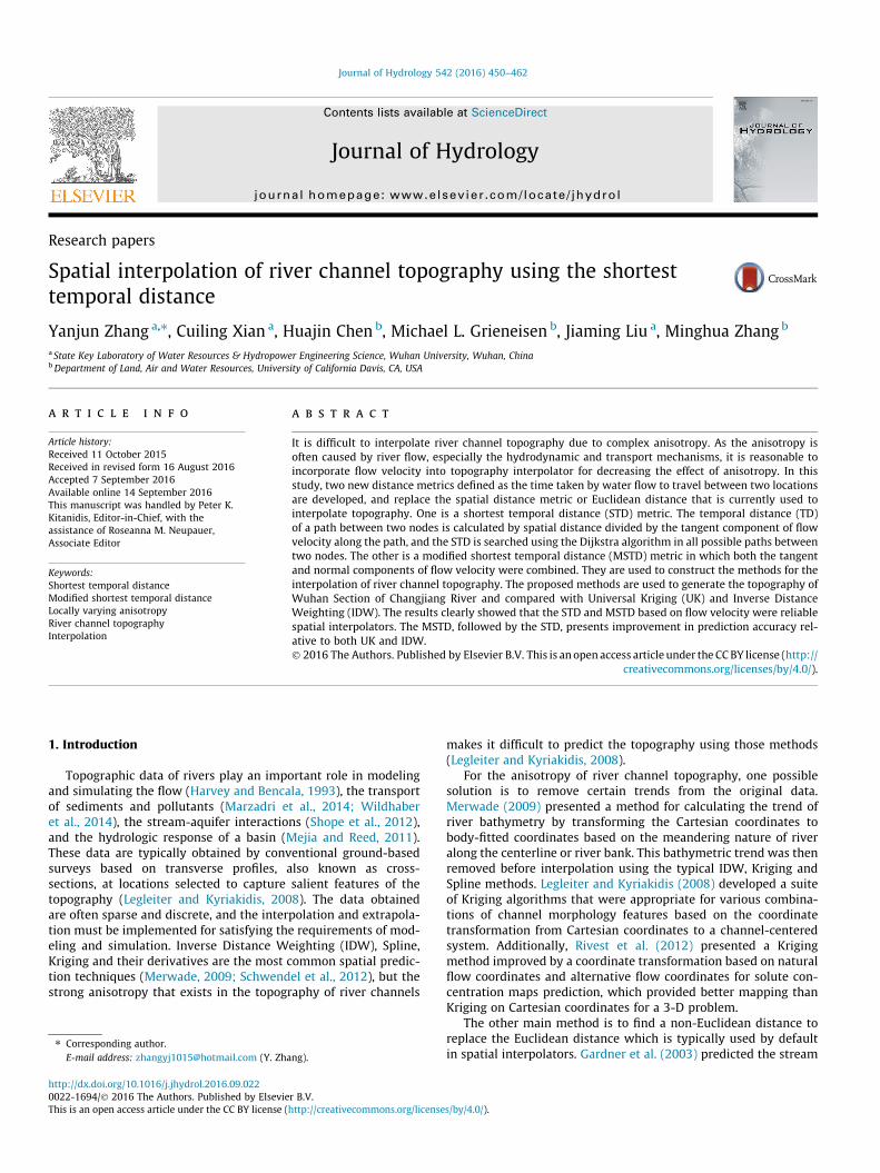
Fig. 1. Wuhan section of the Changjiang River, China.

Y. Zhang et al. / Journal of Hydrology 542 (2016) 450–462 451

temperature by comparing three different geostatistical metrics inKriging: the shortest path, the distances along the stream network,and a modified network system in which the distances wereweighted by stream order. Hoef et al. (2006) developed modelsthat incorporated flow and stream distance by using spatial mov-ing averages, and showed that models using flow might be moreappropriate than models that only use stream distance. Babakand Deutsch (2008) provided an approach to integrate statisticalcontrol into IDW, which could replace the integrated Euclidean dis-tance in IDW, and presented its potential use in the case of vari-ogram misspecification. Boisvert and Deutsch (2011b) presenteda new method for incorporating locally varying anisotropy inKriging and IDW, in which the shortest anisotropic path distance(SPD) between locations was used. Boisvert and Deutsch (2011a)applied this technique in modeling locally varying anisotropy ofCO2 emissions in the United States, and the results showed animprovement in cross validation. Based on the SPD, Li et al.(2014) also developed a method which used shortest wind-fieldpath distance (SWPD) to replace the Euclidean distance in IDW.This method generated estimation surfaces for the particulate mat-ter concentrations in the urban study area.

For all of the approaches implemented in the above studies, thespatial distance was used in the interpolator technique. However,for the river systems, anisotropy is often the result of hydrody-namic or transport mechanisms, and the principal axes of the ani-sotropy are determined by the direction of flow (Kitanidis, 1997).Therefore, the flow velocity may be introduced into topographyinterpolator for decreasing the effect of anisotropy. This studydeveloped a technique for solving the anisotropy of river channeltopography using the temporal distance metrics defined as thetime cost that flow travelled between two nodes. The temporal dis-tance metrics were presented to replace the spatial distances thatare often used in regular spatial interpolators. The correspondinginterpolation methods were developed, and used to predict thetopography of a river channel in the study area. In addition, com-parisons were made among the performances of the STD, MSTD,Universal Kriging (UK) and Inverse Distance Weighting (IDW).

2. Study area

Topography samples of the channel were collected at theWuhan Section of Changjiang River at Wuhan city, Hubei Province,China (Fig. 1). The section is located at the center of ChangjiangRiver downstream of Three Gorges Dam, which is an area of greatconcern to government agencies and the public. The fine-scale andaccurate river channel topography data is critical for a variety ofresearch projects in this important river system. The length ofthe section is 42 km with the mean width 1.8 km. The substratetype is mainly the sandy and silty sediments. The expected resolu-tion of topography is 50 � 50 m, and a 440 � 346 grid was gener-ated to cover the study area, which yielded 22176 valid nodeswithin the river channel. Fig. 2 shows the elevations of the 1183samples (mean 9.8 m and standard deviation 6.53 m), which weresurveyed by the Changjiang Waterway Bureau (CWB) in April2000.

3. Methodology

3.1. The shortest temporal distance method (STD)

In most situations, the default spatial distance (SD) between apair of nodes is calculated by Eq. (1).

SAB ¼ffiffiffiffiffiffiffiffiffiffiffiffiffiffiffiffiffiffiffiffiffiffiDx2 þ Dy2

pð1Þ

where SAB is the spatial distance between nodes A and B (m); Dx andDy are the horizontal and vertical spatial distances between nodes Aand B (m).

For the rivers, the flow is the critical factor causing channeltopographic change, which is obviously distributed along the thal-weg and streamline and is not identical in all spatial directions. Theanisotropy is often the result of hydrodynamic or transport mech-anisms, and the principal axes of the anisotropy are determined bythe direction of flow (Kitanidis, 1997). In this study, a temporal dis-tance is defined as the time cost that the flow travelled between

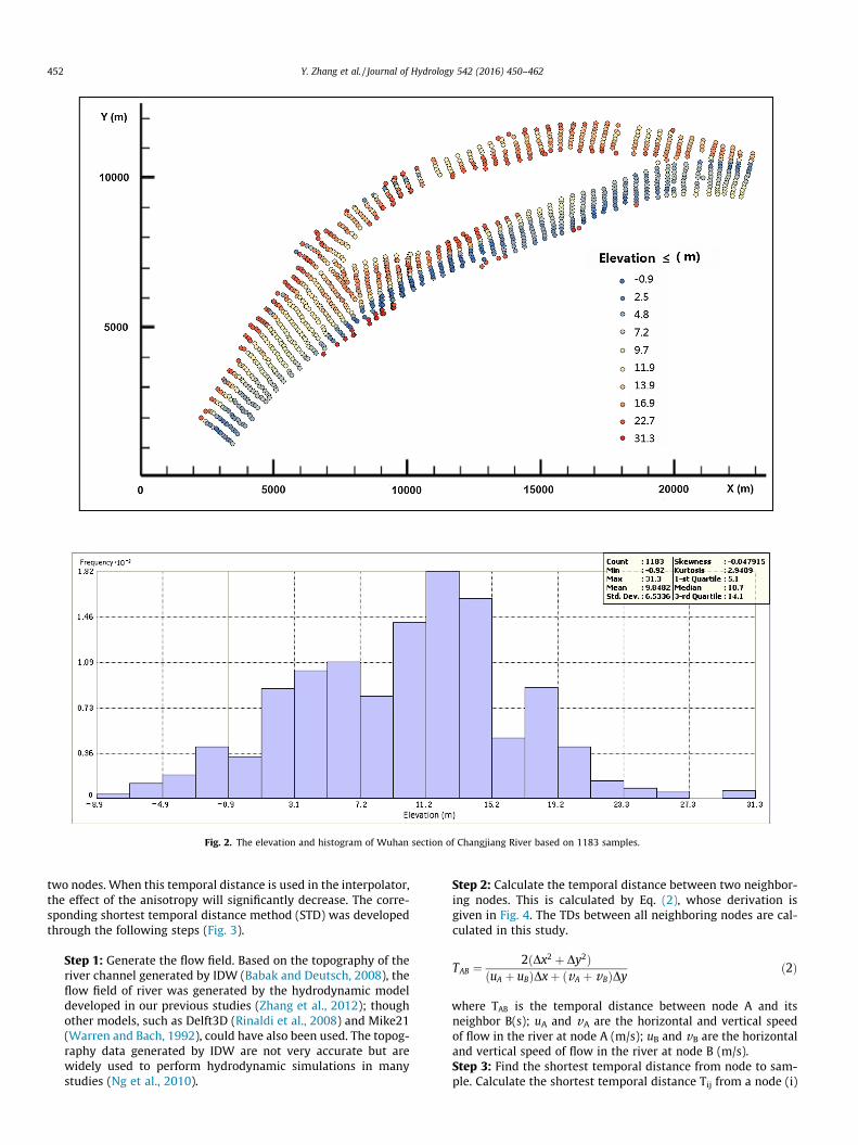
Fig. 2. The elevation and histogram of Wuhan section of Changjiang River based on 1183 samples.

452 Y. Zhang et al. / Journal of Hydrology 542 (2016) 450–462

two nodes. When this temporal distance is used in the interpolator,the effect of the anisotropy will significantly decrease. The corre-sponding shortest temporal distance method (STD) was developedthrough the following steps (Fig. 3).

Step 1: Generate the flow field. Based on the topography of theriver channel generated by IDW (Babak and Deutsch, 2008), theflow field of river was generated by the hydrodynamic modeldeveloped in our previous studies (Zhang et al., 2012); thoughother models, such as Delft3D (Rinaldi et al., 2008) and Mike21(Warren and Bach, 1992), could have also been used. The topog-raphy data generated by IDW are not very accurate but arewidely used to perform hydrodynamic simulations in manystudies (Ng et al., 2010).

Step 2: Calculate the temporal distance between two neighbor-ing nodes. This is calculated by Eq. (2), whose derivation isgiven in Fig. 4. The TDs between all neighboring nodes are cal-culated in this study.

TAB ¼ 2ðDx2 þ Dy2ÞðuA þ uBÞDxþ ðvA þ vBÞDy ð2Þ

where TAB is the temporal distance between node A and itsneighbor B(s); uA and vA are the horizontal and vertical speedof flow in the river at node A (m/s); uB and vB are the horizontaland vertical speed of flow in the river at node B (m/s).Step 3: Find the shortest temporal distance from node to sam-ple. Calculate the shortest temporal distance Tij from a node (i)

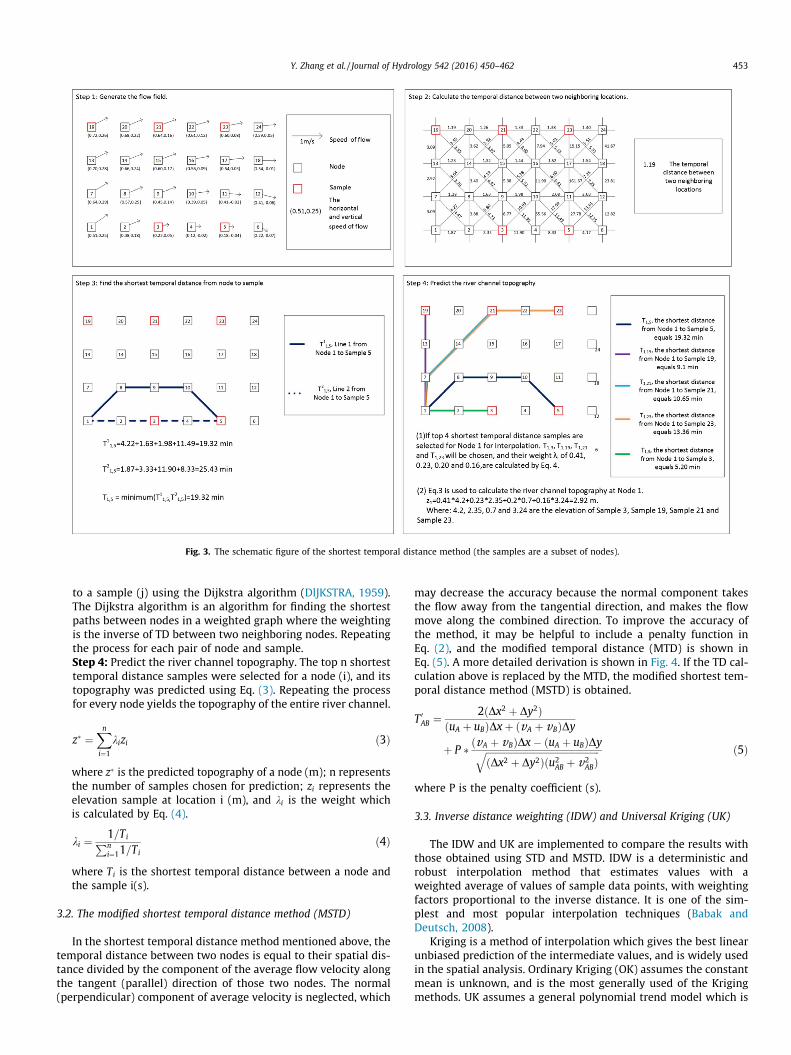
Fig. 3. The schematic figure of the shortest temporal distance method (the samples are a subset of nodes).

Y. Zhang et al. / Journal of Hydrology 542 (2016) 450–462 453

to a sample (j) using the Dijkstra algorithm (DlJKSTRA, 1959).The Dijkstra algorithm is an algorithm for finding the shortestpaths between nodes in a weighted graph where the weightingis the inverse of TD between two neighboring nodes. Repeatingthe process for each pair of node and sample.Step 4: Predict the river channel topography. The top n shortesttemporal distance samples were selected for a node (i), and itstopography was predicted using Eq. (3). Repeating the processfor every node yields the topography of the entire river channel.

z� ¼Xn

i¼1

kizi ð3Þ

where z� is the predicted topography of a node (m); n representsthe number of samples chosen for prediction; zi represents theelevation sample at location i (m), and ki is the weight whichis calculated by Eq. (4).

ki ¼ 1=TiPni¼11=Ti

ð4Þ

where Ti is the shortest temporal distance between a node andthe sample i(s).

3.2. The modified shortest temporal distance method (MSTD)

In the shortest temporal distance method mentioned above, thetemporal distance between two nodes is equal to their spatial dis-tance divided by the component of the average flow velocity alongthe tangent (parallel) direction of those two nodes. The normal(perpendicular) component of average velocity is neglected, which

may decrease the accuracy because the normal component takesthe flow away from the tangential direction, and makes the flowmove along the combined direction. To improve the accuracy ofthe method, it may be helpful to include a penalty function inEq. (2), and the modified temporal distance (MTD) is shown inEq. (5). A more detailed derivation is shown in Fig. 4. If the TD cal-culation above is replaced by the MTD, the modified shortest tem-poral distance method (MSTD) is obtained.

T 0AB ¼ 2ðDx2 þ Dy2Þ

ðuA þ uBÞDxþ ðvA þ vBÞDyþ P � ðvA þ vBÞDx� ðuA þ uBÞDyffiffiffiffiffiffiffiffiffiffiffiffiffiffiffiffiffiffiffiffiffiffiffiffiffiffiffiffiffiffiffiffiffiffiffiffiffiffiffiffiffiffiffiffiffiffiffiffiffi

ðDx2 þ Dy2Þðu2AB þ v2

ABÞq ð5Þ

where P is the penalty coefficient (s).

3.3. Inverse distance weighting (IDW) and Universal Kriging (UK)

The IDW and UK are implemented to compare the results withthose obtained using STD and MSTD. IDW is a deterministic androbust interpolation method that estimates values with aweighted average of values of sample data points, with weightingfactors proportional to the inverse distance. It is one of the sim-plest and most popular interpolation techniques (Babak andDeutsch, 2008).

Kriging is a method of interpolation which gives the best linearunbiased prediction of the intermediate values, and is widely usedin the spatial analysis. Ordinary Kriging (OK) assumes the constantmean is unknown, and is the most generally used of the Krigingmethods. UK assumes a general polynomial trend model which is

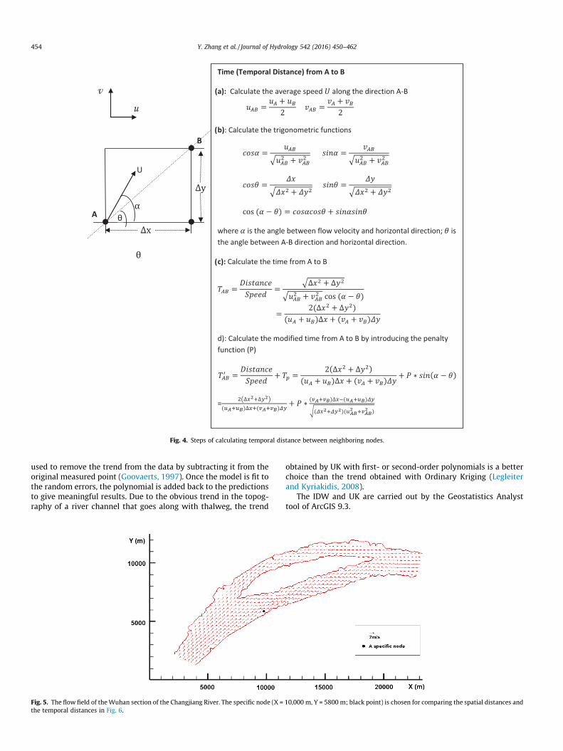
Fig. 4. Steps of calculating temporal distance between neighboring nodes.

454 Y. Zhang et al. / Journal of Hydrology 542 (2016) 450–462

used to remove the trend from the data by subtracting it from theoriginal measured point (Goovaerts, 1997). Once the model is fit tothe random errors, the polynomial is added back to the predictionsto give meaningful results. Due to the obvious trend in the topog-raphy of a river channel that goes along with thalweg, the trend

Fig. 5. The flow field of theWuhan section of the Changjiang River. The specific node (X =the temporal distances in Fig. 6.

obtained by UK with first- or second-order polynomials is a betterchoice than the trend obtained with Ordinary Kriging (Legleiterand Kyriakidis, 2008).

The IDW and UK are carried out by the Geostatistics Analysttool of ArcGIS 9.3.

10,000 m, Y = 5800 m; black point) is chosen for comparing the spatial distances and

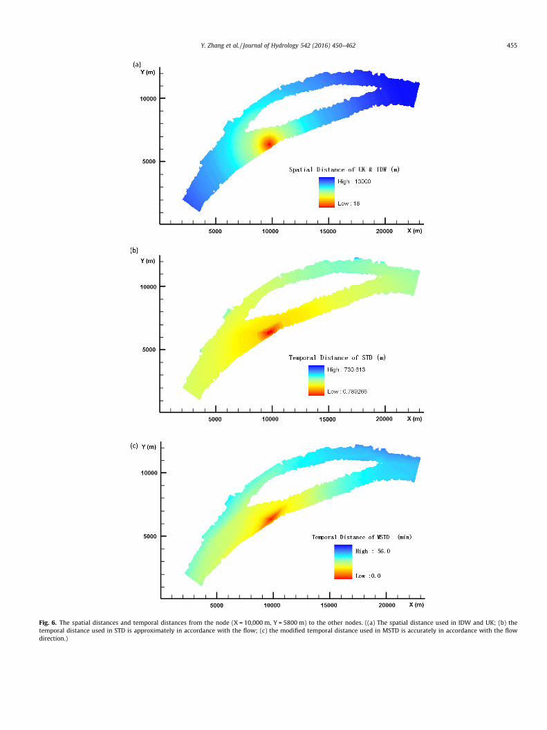
Fig. 6. The spatial distances and temporal distances from the node (X = 10,000 m, Y = 5800 m) to the other nodes. ((a) The spatial distance used in IDW and UK; (b) thetemporal distance used in STD is approximately in accordance with the flow; (c) the modified temporal distance used in MSTD is accurately in accordance with the flowdirection.)

Y. Zhang et al. / Journal of Hydrology 542 (2016) 450–462 455

(a) (b)

(c) (d)

0

20

40

60

80

100

120

140

0 500 1000 1500 2000 2500

Sem

ivar

ianc

e γ

(h)

Distance h (m)

0 Degree Fi�ed Line

0

20

40

60

80

100

120

140

0 500 1000 1500 2000 2500

Sem

ivar

ianc

e γ

(h)

Distance h (m)

0 Degree Fi�ed Line

0

20

40

60

80

100

120

140

0 500 1000 1500 2000 2500

Sem

ivar

ianc

e γ

(h)

Distance h (m)

90 Degree Fi�ed Line

0

20

40

60

80

100

120

140

0 500 1000 1500 2000 2500

Sem

ivar

ianc

e γ

(h)

Distance h (m)

135 Degree Fi�ed Line

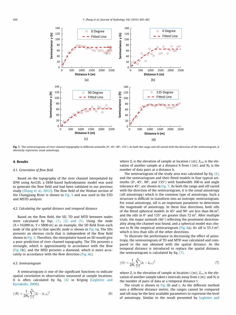
Fig. 7. The semivariograms of river channel topography in different azimuths (0�, 45�, 90�, 135�). As both the range and sill varied with the direction of the semivariogram, itobviously represents zonal anisotropy.

456 Y. Zhang et al. / Journal of Hydrology 542 (2016) 450–462

4. Results

4.1. Generation of flow field

Based on the topography of the river channel interpolated byIDW using ArcGIS, a DEM-based hydrodynamic model was usedto generate the flow field and had been validated in our previousstudy (Zhang et al., 2012). The flow field of the Wuhan section ofthe Changjiang River is shown in Fig. 5 and was used in the STDand MSTD analysis.

4.2. Calculating the spatial distance and temporal distance

Based on the flow field, the SD, TD and MTD between nodeswere calculated by Eqs. (1), (2) and (5). Using the node(X = 10,000 m, Y = 5800 m) as an example, the SD field from eachnode of the grid to that specific node is shown in Fig. 6a. The SDspresents an obvious circle that is independent of the flow fieldshown in Fig. 5. Therefore, the interpolator based on SD would givea poor prediction of river channel topography. The TDs presents arectangle, which is approximately in accordance with the flow(Fig. 6b); and the MSD presents a diamond, which is more accu-rately in accordance with the flow direction (Fig. 6c).

4.3. Semivariogram

A semivariogram is one of the significant functions to indicatespatial correlation in observations measured at sample locations.It is often calculated by Eq. (6) in Kriging (Legleiter andKyriakidis, 2008).

cðhÞ ¼ 12Nh

XNh

i¼1

ðzi � ziþhÞ2 ð6Þ

where Zi is the elevation of sample at location i (m); Zi+h is the ele-vation of another sample at a distance h from i (m); and Nh is thenumber of data pairs at a distance h.

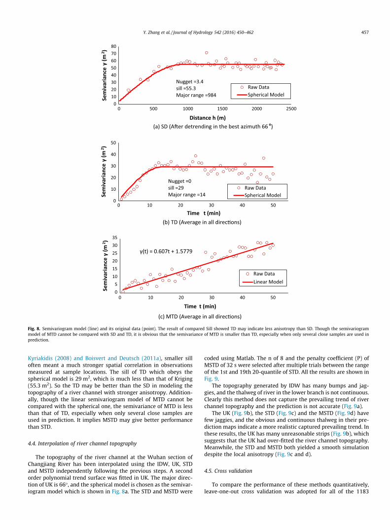
The semivariogram of the study area was calculated by Eq. (6),and the semivariogram and their fitted models in four typical azi-muths (0�, 45�, 90�, and 135�) with bandwidth 300 m and angletolerance 45�, are shown in Fig. 7. As both the range and sill variedwith the direction of the semivariogram, it is the zonal anisotropy(sill anisotropy) which is the common type of anisotropy. Such astructure is difficult to transform into an isotropic semivariogram.For zonal anisotropy, sill is an important parameter to determinethe magnitude of anisotropy. In these four directions, both sillsof the fitted spherical models in 45� and 90� are less than 66 m2,and the sills in 0� and 135� are greater than 72 m2. After multipletrials, the major azimuth (66�) reflecting the prominent direction-ality along the channel was found, and a spherical model was cho-sen to fit the empirical semivariogram (Fig. 8a). Its sill is 55.3 m2,which is less than sills of the other directions.

To illustrate the performance in decreasing the effect of aniso-tropy, the semivariogram of TD and MTD was calculated and com-pared to the one obtained with the spatial distance. As thetemporal distance is introduced to replace the spatial distance,the semivariogram is calculated by Eq. (7).

cðtÞ ¼ 12Nt

XNt

i¼1

ðzi � ziþtÞ2 ð7Þ

where Zi is the elevation of sample at location i (m); Zi+t is the ele-vation of another sample taken t intervals away from i (m); and Nt isthe number of pairs of data at a temporal distance t.

The result is shown in Fig. 8b and c. As the different methoduses a different distance metric, the ranges cannot be comparedand sill may be the best available parameters to represent the levelof anisotropy. Similar to the result presented by Legleiter and

(a) SD (A�er detrending in the best azimuth 66 o)

(b) TD (Average in all direc�ons)

(c) MTD (Average in all direc�ons)

0 1020304050607080

0 500 1000 1500 2000 2500Se

miv

aria

nce

γ (m

2 )

Distance h (m)

Raw DataSpherical Model

Nugget =3.4sill =55.3Major range =984

0

10

20

30

40

50

0 10 20 30 40 50

Sem

ivar

ianc

e γ

(m2 )

Time t (min)

Raw DataSpherical Model

Nugget =0sill =29Major range =14

γ(t) = 0.607t + 1.5779

0 5

101520253035

0 10 20 30 40 50

Sem

ivar

ianc

e γ

(m2 )

Time t (min)

Raw DataLinear Model

Fig. 8. Semivariogram model (line) and its original data (point). The result of compared Sill showed TD may indicate less anisotropy than SD. Though the semivariogrammodel of MTD cannot be compared with SD and TD, it is obvious that the semivariance of MTD is smaller than TD, especially when only several close samples are used inprediction.

Y. Zhang et al. / Journal of Hydrology 542 (2016) 450–462 457

Kyriakidis (2008) and Boisvert and Deutsch (2011a), smaller silloften meant a much stronger spatial correlation in observationsmeasured at sample locations. The sill of TD which obeys thespherical model is 29 m2, which is much less than that of Kriging(55.3 m2). So the TD may be better than the SD in modeling thetopography of a river channel with stronger anisotropy. Addition-ally, though the linear semivariogram model of MTD cannot becompared with the spherical one, the semivariance of MTD is lessthan that of TD, especially when only several close samples areused in prediction. It implies MSTD may give better performancethan STD.

4.4. Interpolation of river channel topography

The topography of the river channel at the Wuhan section ofChangjiang River has been interpolated using the IDW, UK, STDand MSTD independently following the previous steps. A secondorder polynomial trend surface was fitted in UK. The major direc-tion of UK is 66�, and the spherical model is chosen as the semivar-iogram model which is shown in Fig. 8a. The STD and MSTD were

coded using Matlab. The n of 8 and the penalty coefficient (P) ofMSTD of 32 s were selected after multiple trials between the rangeof the 1st and 19th 20-quantile of STD. All the results are shown inFig. 9.

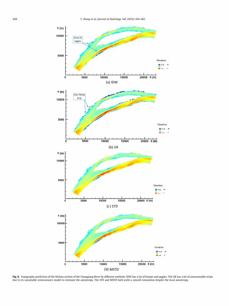
The topography generated by IDW has many bumps and jag-gies, and the thalweg of river in the lower branch is not continuous.Clearly this method does not capture the prevailing trend of riverchannel topography and the prediction is not accurate (Fig. 9a).

The UK (Fig. 9b), the STD (Fig. 9c) and the MSTD (Fig. 9d) havefew jaggies, and the obvious and continuous thalweg in their pre-diction maps indicate a more realistic captured prevailing trend. Inthese results, the UK has many unreasonable strips (Fig. 9b), whichsuggests that the UK had over-fitted the river channel topography.Meanwhile, the STD and MSTD both yielded a smooth simulationdespite the local anisotropy (Fig. 9c and d).

4.5. Cross validation

To compare the performance of these methods quantitatively,leave-one-out cross validation was adopted for all of the 1183

(a) IDW

(b) UK

Bump & Jaggies

Over fi�ng Strip

(c ) STD

(d) MSTD

Fig. 9. Topography prediction of the Wuhan section of the Changjiang River by different methods. IDW has a lot of bumps and jaggies. The UK has a lot of unreasonable stripsdue to its unsuitable semivariance model to estimate the anisotropy. The STD and MSTD both yield a smooth simulation despite the local anisotropy.

458 Y. Zhang et al. / Journal of Hydrology 542 (2016) 450–462

(a) IDW (b) UK

y = 0.7928x + 2.3012R² = 0.8327

-10

-5

0

5

10

15

20

25

-10 0 10 20

Es�m

ate

(m)

Measured (m)

IDW

Standard Line

Fi�ed Line

y = 0.9253x + 0.7912R² = 0.8913

-10

-5

0

5

10

15

20

25

-10 0 10 20

Es�m

ate

(m)

Measured (m)

UK

Standard Line

Fi�ed Line

(c) STD Methods (d) MSTD methods

y = 1.1274x - 1.0092R² = 0.9723

-10

-5

0

5

10

15

20

25

-10 0 10 20

Es�m

ate

(m)

Measured (m)

STD

Standard Line

Fi�ed Line

y = 1.0239x - 0.2256R² = 0.9985

-10

-5

0

5

10

15

20

25

-10.00 -5.00 0.00 5.00 10.00 15.00 20.00 25.00

Es�m

ate

(m)

Measured (m)

STDMStandard LineFi�ed Line

Fig. 10. The comparisons of measured and estimated values for each point by the 4 methods.

Y. Zhang et al. / Journal of Hydrology 542 (2016) 450–462 459

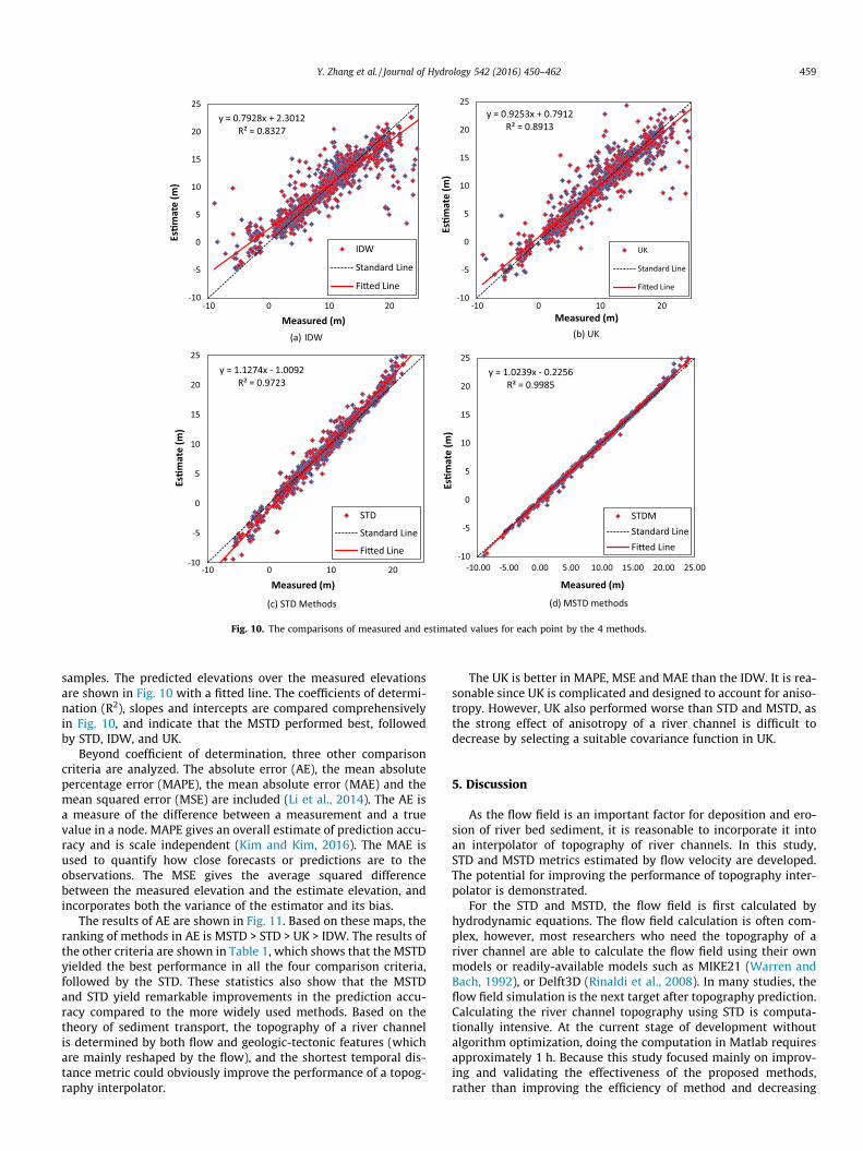
samples. The predicted elevations over the measured elevationsare shown in Fig. 10 with a fitted line. The coefficients of determi-nation (R2), slopes and intercepts are compared comprehensivelyin Fig. 10, and indicate that the MSTD performed best, followedby STD, IDW, and UK.

Beyond coefficient of determination, three other comparisoncriteria are analyzed. The absolute error (AE), the mean absolutepercentage error (MAPE), the mean absolute error (MAE) and themean squared error (MSE) are included (Li et al., 2014). The AE isa measure of the difference between a measurement and a truevalue in a node. MAPE gives an overall estimate of prediction accu-racy and is scale independent (Kim and Kim, 2016). The MAE isused to quantify how close forecasts or predictions are to theobservations. The MSE gives the average squared differencebetween the measured elevation and the estimate elevation, andincorporates both the variance of the estimator and its bias.

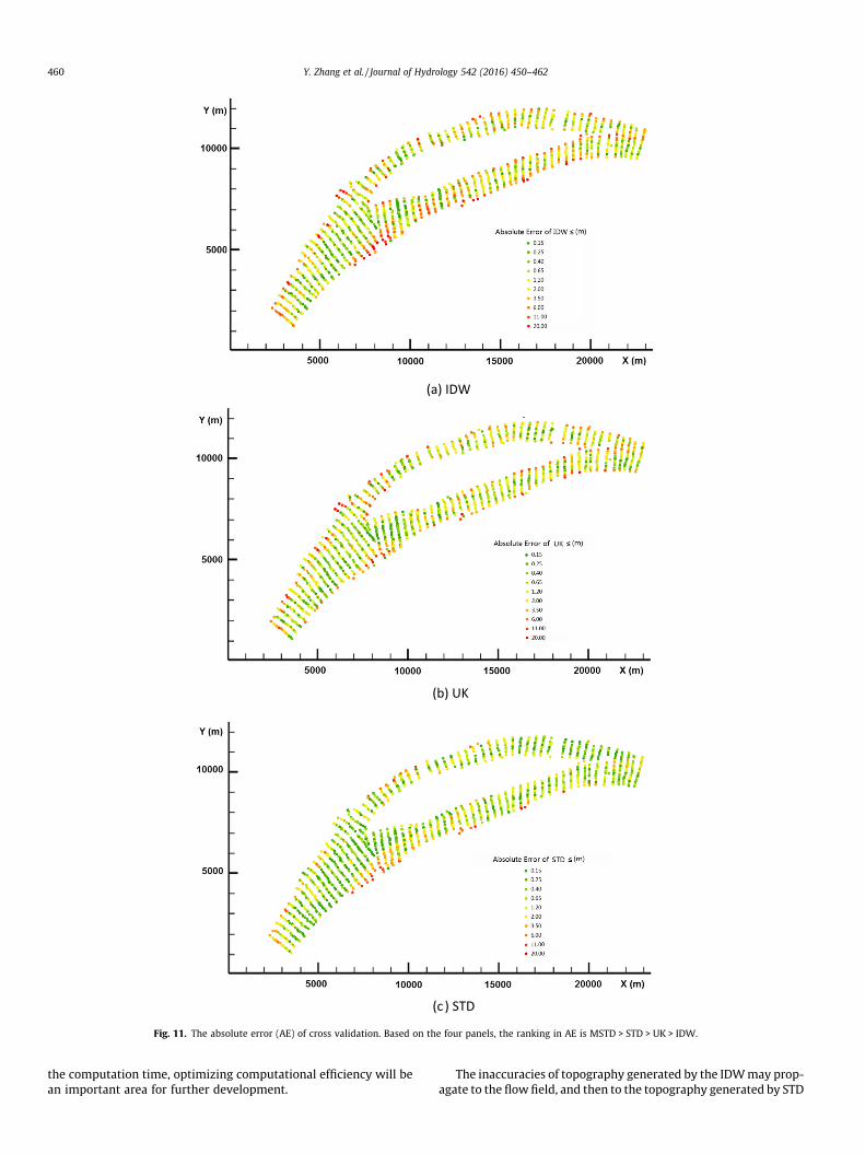
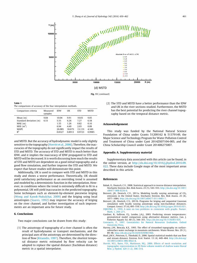
The results of AE are shown in Fig. 11. Based on these maps, theranking of methods in AE is MSTD > STD > UK > IDW. The results ofthe other criteria are shown in Table 1, which shows that the MSTDyielded the best performance in all the four comparison criteria,followed by the STD. These statistics also show that the MSTDand STD yield remarkable improvements in the prediction accu-racy compared to the more widely used methods. Based on thetheory of sediment transport, the topography of a river channelis determined by both flow and geologic-tectonic features (whichare mainly reshaped by the flow), and the shortest temporal dis-tance metric could obviously improve the performance of a topog-raphy interpolator.

The UK is better in MAPE, MSE and MAE than the IDW. It is rea-sonable since UK is complicated and designed to account for aniso-tropy. However, UK also performed worse than STD and MSTD, asthe strong effect of anisotropy of a river channel is difficult todecrease by selecting a suitable covariance function in UK.

5. Discussion

As the flow field is an important factor for deposition and ero-sion of river bed sediment, it is reasonable to incorporate it intoan interpolator of topography of river channels. In this study,STD and MSTD metrics estimated by flow velocity are developed.The potential for improving the performance of topography inter-polator is demonstrated.

For the STD and MSTD, the flow field is first calculated byhydrodynamic equations. The flow field calculation is often com-plex, however, most researchers who need the topography of ariver channel are able to calculate the flow field using their ownmodels or readily-available models such as MIKE21 (Warren andBach, 1992), or Delft3D (Rinaldi et al., 2008). In many studies, theflow field simulation is the next target after topography prediction.Calculating the river channel topography using STD is computa-tionally intensive. At the current stage of development withoutalgorithm optimization, doing the computation in Matlab requiresapproximately 1 h. Because this study focused mainly on improv-ing and validating the effectiveness of the proposed methods,rather than improving the efficiency of method and decreasing

(a) IDW

(b) UK

(c ) STD

Fig. 11. The absolute error (AE) of cross validation. Based on the four panels, the ranking in AE is MSTD > STD > UK > IDW.

460 Y. Zhang et al. / Journal of Hydrology 542 (2016) 450–462

the computation time, optimizing computational efficiency will bean important area for further development.

The inaccuracies of topography generated by the IDWmay prop-agate to the flowfield, and then to the topography generated by STD

(d) MSTD

Fig. 11 (continued)

Table 1The comparisons of accuracy of the four interpolation methods.

Comparison criteria Measuredsamples

IDW UK STD MSTD

Mean (m) 9.84 10.04 9.91 10.03 9.85Standard deviation (m) 6.53 5.55 6.26 7.27 6.58MAE (m) 1.55 1.26 0.82 0.16MSE (m2) 6.94 4.49 2.03 0.08MAPE 26.08% 18.67% 13.11% 4.34%R2 0.8327 0.8913 0.9723 0.9985

Y. Zhang et al. / Journal of Hydrology 542 (2016) 450–462 461

andMSTD. But the accuracy of hydrodynamic model is only slightlysensitive to the topography (Horritt et al., 2006). Therefore, the inac-curacies of the topography do not significantly impact the results ofSTD and MSTD. The accuracy of STD and MSTD is much better thanIDW, and it implies the inaccuracy of IDW propagated to STD andMSTDwill be decreased. It isworth discussing howmuch the resultsof STD and MSTD are dependent on a good initial topography and agood flow simulation, and further improve the STD and MSTD. Weexpect that future studies will demonstrate this point.

Additionally, UK is used to compare with STD and MSTD in thisstudy and shows a worse performance. Theoretically, UK shouldyield satisfactory performance as an overriding trend is assumedand modeled by a deterministic function in the interpolation. How-ever, in conditions where the trend is extremely difficult to fit to apolynomial, UK will yield inaccuracies in the predicted topography.Some techniques such as element-by-element piecewise kriging(Wong and Kanok-Nukulchai, 2009) and the kriging using localanisotropies (Soares, 1992) may improve the accuracy of krigingon the river channel, and further investigation of such improve-ments are an important area for future study.

6. Conclusions

Two major conclusions can be drawn from this study:

(1) The anisotropy of topography of a river channel is often theresult of hydrodynamic or transport mechanisms, and theprincipal axes of the anisotropy are determined by the direc-tion of flow (Kitanidis, 1997). Therefore, the shortest tempo-ral distance metric estimated by flow velocity can beadopted to replace the spatial distance (Euclidean distance)metric in a spatial interpolator.

(2) The STD and MSTD have a better performance than the IDWand UK in the river sections studied. Furthermore, the MSTDhas the best potential for predicting the river channel topog-raphy based on the temporal distance metric.

Acknowledgement

This study was funded by the National Natural ScienceFoundation of China under Grants 51209162 & 51379149, theMajor Science and Technology Program for Water Pollution Controland Treatment of China under Gant 2014ZX07104-005, and theChina Scholarship Council under Grant 201406275007.

Appendix A. Supplementary material

Supplementary data associated with this article can be found, inthe online version, at http://dx.doi.org/10.1016/j.jhydrol.2016.09.022. These data include Google maps of the most important areasdescribed in this article.

References

Babak, O., Deutsch, C.V., 2008. Statistical approach to inverse distance interpolation.Stochastic Environ. Res. Risk Assess. 23 (5), 543–553. http://dx.doi.org/10.1007/s00477-008-0226-6.

Boisvert, J.B., Deutsch, C.V., 2011a. Modeling locally varying anisotropy of CO2

emissions in the United States. Stochastic Environ. Res. Risk Assess. 25 (8),1077–1084. http://dx.doi.org/10.1007/s00477-011-0483-7.

Boisvert, J.B., Deutsch, C.V., 2011b. Programs for kriging and sequential Gaussiansimulation with locally varying anisotropy using non-Euclidean distances.Comput. Geosci. 37 (4), 495–510. http://dx.doi.org/10.1016/j.cageo.2010.03.021.

DlJKSTRA, E., 1959. A note on two problems in connexion with graphs. Numer.Math. 1, 269–271.

Gardner, B., Sullivan, P.J., Lembo, J.A.J., 2003. Predicting stream temperatures:geostatistical model comparison using alternative distance metrics. Can. J.Fisheries Aquatic Sci. 60 (3), 344–351. http://dx.doi.org/10.1139/f03-025.

Goovaerts, P., 1997. Geostatistics for Natural Resources Evaluation. OxfordUniversity Press.

Harvey, J.W., Bencala, K.E., 1993. The effect of streambed topography on surface-subsurface water exchange in mountain catchments. Water Resour. Res. 29 (1),89–98. http://dx.doi.org/10.1029/92WR01960.

Hoef, J.M.V., Peterson, E., Theobald, D., 2006. Spatial statistical models that use flowand stream distance. Environ. Ecol. Statist. 13 (4), 449–464. http://dx.doi.org/10.1007/s10651-006-0022-8.

Horritt, M.S., Bates, P.D., Mattinson, M.J., 2006. Effects of mesh resolution andtopographic representation in 2D finite volume models of shallow water fluvialflow. J. Hydrol. 329 (1–2), 306–314.

462 Y. Zhang et al. / Journal of Hydrology 542 (2016) 450–462

Kim, S., Kim, H., 2016. A new metric of absolute percentage error for intermittentdemand forecasts. Int. J. Forecasting 32 (3), 668–679.

Kitanidis, P., 1997. Introduction to Geostatistics: Applications in Hydrogeology.Cambridge University Press.

Legleiter, C.J., Kyriakidis, P.C., 2008. Spatial prediction of river channel topographyby kriging. Earth Surf. Processes Landforms 33 (6), 841–867. http://dx.doi.org/10.1002/esp.1579.

Li, L., Gong, J., Zhou, J., 2014. Spatial interpolation of fine particulate matterconcentrations using the shortest wind-field path distance. PloS one 9 (5),e96111. http://dx.doi.org/10.1371/journal.pone.0096111.

Marzadri, A., Tonina, D., Bellin, A., Tank, J.L., 2014. A hydrologic model demonstratesnitrous oxide emissions depend on streambed morphology. Geophys. Res. Lett.41 (15), 5484–5491.

Mejia, A., Reed, S., 2011. Role of channel and floodplain cross-section geometry inthe basin response. Water Resour. Res. 47 (9), W09518. http://dx.doi.org/10.1029/2010WR010375.

Merwade, V., 2009. Effect of spatial trends on interpolation of river bathymetry. J.Hydrol. 371 (1–4), 169–181. http://dx.doi.org/10.1016/j.jhydrol.2009.03.026.

Ng, S.M.N., Wai, O.W.H., Xu, Z.H., Li, Y.S., 2010. Integrating GIS with HydrodynamicModel for Wastewater Disposal and Management: Pearl River Estuary. 13, pp.207–217. http://dx.doi.org/10.1007/978-1-4020-9720-1_19.

Rinaldi, M., Mengoni, B., Luppi, L., Darby, S.E., Mosselman, E., 2008. Numericalsimulation of hydrodynamics and bank erosion in a river bend. Water Resour.Res. 44 (9).

Rivest, M., Marcotte, D., Pasquier, P., 2012. Sparse data integration for theinterpolation of concentration measurements using kriging in naturalcoordinates. J. Hydrol. 416–417, 72–82. http://dx.doi.org/10.1016/j.jhydrol.2011.11.043.

Schwendel, A.C., Fuller, I.C., Death, R.G., 2012. Assessing DEM interpolation methodsfor effective representation of upland stream morphology for rapid appraisal ofbed stability. River Res. Appl. 28 (5), 567–584. http://dx.doi.org/10.1002/rra.1475.

Shope, C., Constantz, J., Cooper, C., Reeves, D., Pohll, G., McKay, W., 2012. Influenceof a large fluvial island, streambed, and stream bank on surface water-groundwater fluxes and water table dynamics. Water Resour. Res. 48 (6),W06512. http://dx.doi.org/10.1029/2011WR011564.

Soares, C., 1992. Geostatistical estimation of multi-phase structures. Math. Geol. 24(2), 149–160.

Warren, I.R., Bach, H., 1992. MIKE 21: a modelling system for estuaries, coastalwaters and seas. Environ. Software 7 (4), 229–240.

Wildhaber, Y.S., Michel, C., Epting, J., Wildhaber, R.A., Huber, E., Huggenberger, P.,Alewell, C., 2014. Effects of river morphology, hydraulic gradients, and sedimentdeposition on water exchange and oxygen dynamics in salmonid redds. Sci.Total Environ. 470, 488–500.

Wong, F., Kanok-Nukulchai, W., 2009. Kriging-based finite element method:element-by-element Kriging interpolation. Civ. Eng. Dimension 11 (1), 15–22.

Zhang, Y.J., Jha, M., Gu, R., Wensheng, L., Alin, L., 2012. A DEM-based parallelcomputing hydrodynamic and transport model. River Res. Appl. 28 (5), 647–658. http://dx.doi.org/10.1002/rra.1471.