spatial ecology and life-history diversity of snake …
TRANSCRIPT

SPATIAL ECOLOGY AND LIFE-HISTORY DIVERSITY OF SNAKE RIVER
FINESPOTTED CUTTHROAT TROUT ONCORHYNCHUS CLARKII
BEHNKEI IN THE UPPER SNAKE RIVER, WY
by
Kristen Michele Homel
A dissertation submitted in partial fulfillment of the requirements for the degree
of
Doctor of Philosophy
in
Fish and Wildlife Biology
MONTANA STATE UNIVERSITY Bozeman, Montana
April 2013

©COPYRIGHT
by
Kristen Michele Homel
2013
All Rights Reserved

ii
APPROVAL
of a dissertation submitted by
Kristen Michele Homel
This dissertation has been read by each member of the dissertation committee and has been found to be satisfactory regarding content, English usage, format, citation, bibliographic style, and consistency and is ready for submission to The Graduate School.
Dr. Wyatt Cross
Approved for the Department of Ecology
Dr. David Roberts
Approved for The Graduate School
Dr. Ronald W. Larsen

iii
STATEMENT OF PERMISSION TO USE
In presenting this dissertation in partial fulfillment of the requirements for a
doctoral degree at Montana State University, I agree that the Library shall make it
available to borrowers under rules of the Library. I further agree that copying of this
dissertation is allowable only for scholarly purposes, consistent with “fair use” as
prescribed in the U.S. Copyright Law. Requests for extensive copying or reproduction of
this dissertation should be referred to ProQuest Information and Learning, 300 North
Zeeb Road, Ann Arbor, Michigan 48106, to whom I have granted “the exclusive right to
reproduce and distribute my dissertation in and from microform along with the non-
exclusive right to reproduce and distribute my abstract in any format in whole or in part.”
Kristen Michele Homel April 2013

iv
DEDICATION
I dedicate this dissertation to my parents, Steven and Terry, and my siblings, Jen, Mike, and Lisa, who have supported and encouraged me in all my endeavors, and to Benny, my dearest friend.

v
ACKNOWLEDGEMENTS
This project could not have happened without the cooperation, financial support,
field assistance, and intellectual feedback from many, many people. Funding was
provided by the National Fish and Wildlife One Fly program, the U.S. Geological
Survey, the National Park Service, and the National Park Service-University of Wyoming
AMK research station. Special thanks goes to Patrick Connolly, Brady Allen, and Philip
Haner, with the U.S. Geological Survey Columbia River Research Laboratory, for
providing telemetry equipment, instruction on radio-tagging, and expertise in installing
radio antennae.
Thank you to my major advisor, Bob Gresswell, and committee members, Wyatt
Cross, Jeff Kershner, and Tom McMahon for the stimulating learning environment, long
conversations, and professional development. I am so grateful for your time and
mentoring.
Thank you to Ted Sedell, Katie Franz, Jacob Stoller, Bonnie Griffis, Sam Bourret,
Lora Tennant, Rob Gipson, Tracy Stephens, Diana Sweet, Jim Gregory, Dave Stinson,
Sue O’Ney, and numerous volunteers for assistance with field work and insight into the
project. Lynn DiGennaro provided administrative assistance, endless reassurance,
positive energy, and candy.
Finally, I would like to thank my lab mates and friends in Bozeman, MT and
Jackson Hole, WY. You made the experience incredible. I hope our paths continue to
cross and this time together was just the beginning.

vi
TABLE OF CONTENTS
1. INTRODUCTION TO DISSERTATION .......................................................................1
Introduction ......................................................................................................................1 Background ......................................................................................................................5 Threats to Persistence ......................................................................................................8 Overview of Chapters ......................................................................................................9 References Cited ............................................................................................................13 2. LIFE-HISTORY DIVERSITY OF SNAKE RIVER FINESPOTTED CUTTHROAT
TROUT IN THE UPPER SNAKE RIVER: IMPLICATIONS FOR THE CONSERVATION OF NATIVE TROUT IN A LARGE RIVER NETWORK ..........20
Abstract ..........................................................................................................................20 Introduction ....................................................................................................................21 Methods..........................................................................................................................25 Results ............................................................................................................................30 Discussion ......................................................................................................................34 Acknowledgments..........................................................................................................39 Figures............................................................................................................................41 Tables .............................................................................................................................46 References ......................................................................................................................48 3. INTERPOLATING PROBABILISTIC MOVEMENT PATHS FROM SPARSE TELEMETRY DATA IN A LINEAR SYSTEM ..........................................................55
Abstract ..........................................................................................................................55 Introduction ....................................................................................................................56 Methods..........................................................................................................................59 Adaptive Kernel Density Interpolation (AKDI) Method ........................................59 Linear Interpolation ................................................................................................61 Fixed Kernel Density ..............................................................................................61 Comparing Interpolation Methods ..........................................................................62 Results ............................................................................................................................62 Discussion ......................................................................................................................63 Acknowledgments..........................................................................................................67 Figures............................................................................................................................69 References ......................................................................................................................72

vii
TABLE OF CONTENTS - CONTINUED 4. SCALING UP: SPATIAL AND HIERARCHICAL VARIATION IN MOVEMENT
AND HABITAT OCCUPANCY PATTERNS OF CUTTHROAT TROUT IN THE UPPER SNAKE RIVER, WY.......................................................................................75
Abstract ..........................................................................................................................75 Introduction ....................................................................................................................76 Methods..........................................................................................................................80
Spatiotemporal Movement Patterns .......................................................................83 Habitat Relationships .............................................................................................84
Results ............................................................................................................................87 Spatiotemporal Movement Patterns .......................................................................88 Habitat Relationships .............................................................................................88
Discussion ......................................................................................................................90 Acknowledgments..........................................................................................................97 Figures............................................................................................................................98 Tables ...........................................................................................................................104 References ....................................................................................................................111 5. SYNTHESIS AND CONCLUSIONS .........................................................................117
Principle Findings ........................................................................................................118
Summary .....................................................................................................................121 References ...................................................................................................................123
REFERENCES CITED ....................................................................................................126 APPENDICES .................................................................................................................142
Appendix A. Calculating Utilization Distributions ....................................................143 Appendix B. Probability Field Underlying AKDI Kernels ........................................146 Appendix C. Annotated Model Code for Simulations ...............................................148 Appendix D. Annotated Model Code for Applying AKDI ........................................170

viii
LIST OF TABLES
Table Page
2.1. Total number of Snake River finespotted cutthroat trout Oncorhynchus
clarki behnkei captured and radio-tagged in segments of the Snake River between Jackson Lake Dam and Moose Junction in 2007 and 2008. Average and range of total length is summarized by river segment. .............46
2.2. Spawning date, location, and habitat type (tributary, spring creek, or side
channel) for 140 Snake River finespotted cutthroat trout Oncorhynchus
clarki behnkei that made distinct spawning migrations in 2008 and/or 2009 in the upper Snake River watershed below Jackson Lake Dam. Springs designated as “left” or “right” are on river left or right, when looking downstream. ......................................................................................47
4.1. Physical habitat attributes (and associated method and reference) recorded
in the upper Snake River during 2009 or derived using GIS based on 2009 LIDAR data .........................................................................................104
4.2. Reach occupancy by radio-tagged Snake River finespotted cutthroat trout
Oncorhynchus clarkii behnkei and physical characteristics of each stream reach in the upper Snake River from Jackson Lake Dam to Moose Junction, 2009 ..............................................................................................105
4.3. Correlation matrix of environmental attributes in the upper Snake River
below Jackson Lake Dam, 2009. Only variables with a correlation less than 0.7 were retained combined in regression models ................................107
4.4. Candidate regression models to evaluate the relationship between habitat
occupancy and reach-scale habitat attributes for Snake River finespotted cutthroat trout Oncorhynchus clarkii behnkei in the upper Snake River, WY 2009. The Full dataset and Segments 2-6 datasets were evaluated with mixed effects models where segments were modeled as a random intercept. The Segment 1 dataset was evaluated with fixed effects models. Akaike’s information criterion (AIC) are presented for all models. The AIC (difference from top model) and r2 value (for the linear regression models with the Segment 1 dataset) are presented for models where all variables were significant. Segment 1 models were not nested, so AIC values were not presented. LWD = large woody debris, Depth = maximum depth, Banks = bank structure, and Mac = macrophytes. ...............................................................................................108

ix
LIST OF TABLES – CONTINUED
Table Page
4.5. Top regression models to evaluate the relationship between habitat occupancy and reach-scale habitat attributes for Snake River finespotted cutthroat trout Oncorhynchus clarkii behnkei in the upper Snake River, WY 2009. Mixed effects models were constructed for the Full and Segments 2-6 datasets, with segment as the grouping variable. Fixed effects models were constructed for the Segment 1 dataset. Parameter estimates, parameter transformations, standard error (SE), and significance (p-value) are presented for the top regression model(s) for each dataset (Full dataset = segments 1-6). ..................................................110

x
LIST OF FIGURES
Figure Page
1.1. Mean daily discharge (cubic meters per second; CMS) recorded at the USGS gage (Moran, WY) immediately below Jackson Lake Dam for the periods of time 1910-1957 (prior to construction of Palisades Dam) and 1959-2007 (beginning after full pool was reached in Palisades Reservoir) and the estimated unregulated mean daily discharge that would be released from Jackson Lake in the absence of Jackson Lake Dam. ...............11
1.2. Discharge (cubic meters per second; CMS) recorded at Moose Junction
on the Snake River, 2002-2009. Solid lines are years when peak discharge is > 283 CMS (corresponding to 10,000 CFS) dashed lines are years when peak discharge is < 283 CMS. .....................................................12
1.3. Estimated discharge (cubic meters per second; CMS) at Moose Junction
on the Snake River that would occur in the absence of Jackson Lake Dam, 2002-2009. Estimated discharge is sum of (1) the estimated discharge at Jackson Lake Dam produced by the Bureau of Reclamation, (2) the discharge recorded at Pacific Creek, and (3) the discharge recorded at Buffalo Fork. Solid lines are years when peak discharge is > 283 CMS (corresponding to 10,000 CFS) dashed lines are years when peak discharge is < 283 CMS .........................................................................12
2.1. Snake River study area from Jackson Lake Dam to Palisades Reservoir,
Wyoming. Major tributaries are labeled, and sample segments classified for habitat surveys are labeled and delineated with unique colors. Tagging locations of Snake River finespotted cutthroat trout Oncorhynchus Clarkii Behnkei are shown as red dots. ..................................41
2.2. Fig Discharge (cubic meters per second; m3/s) and mean temperature
(Celsius; C) recorded at the USGS Moose Junction gauging station on the Snake River from July 1, 2007 to November 15, 2009. Snake River finespotted cutthroat trout Oncorhynchus clarkii behnkei were radio-tagged during September and October of 2007 and 2008 (grey bars) and relocated until November of 2009. .................................................................42
2.3. Percent composition of habitat types within each segment (n = 12) of the
Snake River from Jackson Lake Dam (the top of segment A) to Palisades Reservoir (the bottom of segment L). Habitat can be Constrained (C) with Levied (L) or Natural (N) banks, Unconstrained (U), and with a channel geometry of Single (S), Multiple (M), or Braided (B) channels ....................43

xi
LIST OF FIGURES – CONTINUED
Figure Page 2.4. Location of radio-tagged Snake River finespotted cutthroat trout
Oncorhynchus clarkii behnkei in the Snake River and tributaries during the prespawning (October; panel A), spawning (panel B), and postspawning (September; panel C) periods. Individual spawners are color-coded by life-history strategy (fluvial = orange, fluvial-adfluvial spring = pale blue, and fluvial-adfluvial tributary = green) ...........................44
2.5. Percent of each movement pattern expressed by radio-tagged Snake River
finespotted cutthroat trout Oncorhynchus clarkii behnkei in the upper Snake River in each spawn location. Movement type 1 are individuals that spawned in the segment in which they were tagged, type 2 returned to the tag segment postspawning, and type 3 did not return to the tag segment postspawning. Only locations where individuals survived postspawning are included and locations marked with “*” indicate a single observation ....45
3.1. Two potential movement paths (A and B) connecting identical relocation
points (panel A) with the corresponding patterns of space-use frequency generated from sample points contrasted against the actual utilization distribution of each movement path (panel B). ..............................................69
3.2. Interpolated probability of time spent along a continuous path through X
(location)-t (time) space generated using the adaptive kernel density interpolation method (AKDI). The height of the plot corresponds to the probability of time spent in a particular location at a particular time. ...........70
3.3. Root mean square error of the adaptive kernel density interpolation method
(AKDI), naive sample data, linear interpolation, and fixed kernel density across sample sizes ranging from 5 to 100. ....................................................71
4.1. Snake River study area from Jackson Lake Dam to Moose Junction, WY.
Major tributaries are labeled, and sample segments classified for habitat surveys are labeled and reaches are delineated with unique colors. Tagging locations of Snake River finespotted cutthroat trout Oncorhynchus clarkii behnkei are shown as red dots. ...................................98
xii
LIST OF FIGURES – CONTINUED
Figure Page 4.2. Discharge (cubic meters per second; m3/s) and mean temperature
(Celsius; C) recorded at the USGS Moose Junction gauging station on the Snake River from July 1, 2007 to November 15, 2009. Snake River finespotted cutthroat trout Oncorhynchus clarkii behnkei were radio-tagged during September and October of 2007 and 2008 (grey bars) and relocated through October, 2009 ....................................................................99
4.3. Percent of radio-tagged Snake River finespotted cutthroat trout
Oncorhynchus clarkii behnkei moving each month at the reach (dashed line) and segment scales (solid line) in 2007 (red line) and 2008 (blue line) in the upper Snake River ,WY .............................................................100
4.4. Percent of radio-tagged Snake River finespotted cutthroat trout
Oncorhynchus clarkii behnkei moving during base flow (October 1 – April 14), runoff (April 15 – July 31), and post-runoff (August 1 – September 30) at the reach (dashed line) and segment scales (solid line) in 2007 (red line) and 2008 (blue line) in the upper Snake River ,WY .......100
4.5. Annual sum of monthly movement distances (in reaches) by radio-tagged
Snake River finespotted cutthroat trout Oncorhynchus clarkii behnkei (n = 94) in the Snake River, WY October 2007 – September 2009. ................101
4.6. Annual sum of monthly movement distances (in segments) by radio-
tagged Snake River finespotted cutthroat trout Oncorhynchus clarkii
behnkei (n = 94) in the Snake River, WY October 2007 – September 2009. .............................................................................................................101
4.7. Monthly reach occupancy of radio-tagged cutthroat trout Oncorhynchus
clarkii behnkei (n = 94) in the upper Snake River, WY October 2008 – September 2009. Monthly reach occupancy represents the total amount of time spent in each reach during each month by all individuals, collectively.. .................................................................................................102

xiii
LIST OF FIGURES – CONTINUED
Figure Page 4.8. Principle coordinates analysis of monthly utilization distributions for all
radio-tagged Snake River finespotted cutthroat trout Oncorhynchus
clarkii behnkei combined. The first component explained 99% of the variation among monthly utilization distributions and described differences in spatial patterns of time spent. The second component explained 1% of the variation and described differences between winter and summer utilization distributions. ...........................................................103
6.1. Method to calculate discrete utilization distributions from continuous
movement paths (Appendix A). ...................................................................144
6.2. Probability field contours surrounding an interpolated path generated using the adaptive kernel density interpolation method (Appendix B). .......147

xiv
ABSTRACT Life-history diversity, movement patterns, and habitat associations of cutthroat
trout Oncorhynchus clarkii have been widely studied in smaller river systems and are critical components of conservation planning. However, much less is known about how the patterns observed in smaller systems may “scale up” in larger, complex river systems. In my dissertation, I evaluated the life-history variation and spatial ecology of Snake River finespotted cutthroat trout O. c. behnkei in the upper Snake River, WY and collaborated on a statistical method to characterize habitat occupancy from radio-telemetry data. For my first chapter, I identified the life-history diversity and movement patterns of cutthroat trout in a large river network using radio-telemetry. Spawning occurred from May through July throughout the upper Snake River in spring creeks, tributaries, and side channels over a spatial extent > 100 km. Postspawning movement patterns varied among spawning areas and life-history forms. Results indicated that life-history diversity in large river networks is substantially more complex than may be observed in headwater systems, reflecting increased habitat complexity and availability in larger systems. For my second chapter, I collaborated on a method to address three biases in radio-telemetry datasets: (1) data may be collected at sparse, unequal sampling intervals, (2) encountering an individual in a location does not imply occupancy, and (3) all locations between where individuals are encountered are occupied to some extent, despite the lack of observations. The resulting adaptive kernel density interpolation method treated location as a utilization distribution for each tracking interval (e.g., a week) and estimated time spent per location as a function of individual movement speed and time since last relocation. For my third chapter, I evaluated habitat occupancy and movement patterns at multiple spatiotemporal scales. Spatial variation and hierarchical structure in the physical template interacted to produce contextual variation in the availability and function of habitat attributes (e.g., wood functioning as cover or as a velocity break). Collectively, these studies provide a more complete understanding of life-history diversity in a large river network and the way in which variation in the physical template shapes habitat occupancy, and movement patterns.

1
INTRODUCTION TO DISSERTATION
Introduction
Over the last century, native trout have experienced dramatic declines in
distribution and abundance as a result of habitat degradation, fragmentation, invasive
species, and hybridization (Gresswell et al. 1988; Miller et al. 1989; Hudy et al. 2007).
Many rivers have been dammed, channelized, or simplified, and access to habitat
associated with different life stages or life-history strategies has been lost (Thurow et al.
1997; Fausch et al. 2002). Declines have been particularly pronounced for riverine
migratory fish that rely on intact corridors to access seasonal habitat and encounter more
degraded habitat in the course of migration (Thurow et al. 1997). In response to these
declines, conservation of native trout has focused on factors that promote population
resiliency, including life-history diversity (Gresswell et al. 1994; Rieman and Dunham
2000) and habitat patch size (Hilderbrand and Kershner 2000a). Each of these factors is
closely associated with characteristics of the physical template (Southwood 1977; Poff
and Ward 1990). However, the template is dynamic, patchy, and hierarchical (Frissell et
al. 1986; Poole 2002; Thorp et al. 2006), which hinders predictions of a population-level
response over time or across systems.
Life-history variation describes traits associated with survival and reproduction
and relates directly to variation in the physical template; where a greater diversity of
habitat types are available, a greater diversity of life histories may be expressed to
connect those habitat types with movement (Cole 1954; Stearns 1977). Life-history

2 variation is linked to population resilience (Hilborn et al. 2003) through spreading of
extirpation risk through space and time (Den Boer 1968; Stearns 1989; Greene et al.
2010). For example, spawning behaviors are often associated with temporary occupation
of spatially discrete seasonal habitats (e.g., lake or tributary spawning areas; Gresswell et
al. 1994). When multiple spawning behaviors are present in a population, disturbance at
the local scale might only cause extirpation of the portion of the population currently
associated with the affected habitat (Den Boer 1968). Subsequently, recolonization may
occur by other individuals from the same population over time (Rieman et al. 1997;
Gresswell 1999). Life-history sets the context for understanding the specific habitats
required by trout, but the physical template determines the availability, quality, and
spatiotemporal occupancy of those habitats.
Efforts to understand how trout respond to the physical template have advanced in
both spatially implicit and spatially explicit directions, and the characteristics of each
differ in important ways. In spatially implicit models, habitat use is described in terms of
the habitat patches that individuals connect with movement through corridors (Schlosser
and Angermeier 1995; Northcote 1997); the specific habitat occupied may differ
seasonally (Fretwell 1972), by life stage, by life-history form, and by species (Schlosser
1991; Northcote 1997). Moreover, the physical template of a stream network influences
fish distribution patterns at hierarchical spatial scales (Levin 1992; Rabeni and Sowa
1996; Lowe et al. 2006). At broad scales (e.g., watershed), physical attributes, such as
watershed connectivity (MacArthur and Wilson 1967; Hitt and Angermeier 2006;
Muneepeerakul et al. 2008), stream network topology and complexity (Cuddington and

3 Yodzis 2002; Benda et al. 2004; Grant et al. 2007), and temperature (Torgersen et al.
2006) or gradient (Kruse et al. 1997) are directly related to habitat suitability and access.
Conversely, at local scales (e.g., reach), fish distribution may be influenced by physical
structure (e.g., large woody debris; Abbe and Montgomery 1996), and thermal or velocity
refugia (Torgersen et al. 1999; Ebersole et al. 2003). Although these spatially implicit
models may be useful for identifying habitat relationships, they tend to do an inadequate
job of predicting fish-habitat relationships in different locations within a stream or
different streams.
Recently, there has been a greater emphasis on the importance of spatially explicit
processes in stream systems (Fausch et al. 2002; Weins 2002; Carbonneau et al. 2011).
In spatially explicit models, habitat use incorporates both position within the stream
network (resulting from major downstream changes in the biophysical characteristics of
streams; Vannote et al. 1980) and heterogeneity (because local physical heterogeneity
may be greater than longitudinal variation in the stream at smaller spatial scales; Poole
2002; Ganio et al. 2005; Thorp et al. 2006). The location within the stream network sets
the context of how different types of habitat or habitat forming processes may occur in
different portions of the watershed and structure fish distribution or abundance.
Consequently, a riverscapes perspective allows integration of how life cycles are linked
to habitat characteristics in specific locations within a watershed (Fausch et al. 2002).
Much of the work on life-history diversity or habitat occupancy of trout has been
conducted in headwater systems or lake-stream systems (Hilderbrand and Kershner
2000b; Brown and Mackay 1995; Gresswell 2011), partly because there are few large

4 river systems where migration is still possible throughout a complex network of streams.
This bias toward studies in smaller streams has resulted in generalizations about habitat
use or movement patterns that may be true of smaller systems but may not apply in larger
systems. For example, it appears that trout connect seasonal habitat with shorter
movements in smaller streams than in larger rivers (Colyer et al. 2005; Gresswell and
Hendricks 2007), suggesting that attributes of the physical template associated with that
movement differ. However, it is not enough to identify that individuals move longer
distances in larger streams without considering how those movements, and subsequent
habitat occupation, are products of stream-size specific habitat availability, quality, and
spatial arrangement.
Large river networks differ physically from small streams in several ways that
could potentially influence fish distribution and habitat use patterns. Large rivers display
a greater range of network topologies than small streams, and the spatial pattern of
tributary confluences of varying size could affect the spatial availability of habitat (Benda
et al. 2004; Torgersen et al. 2008). Irrespective of the topology, fewer tributary
confluences are large enough relative to the main stem to impart a geomorphic effect that
could form seasonal or annual habitat at the confluence (Benda et al. 2004). Hence
segments tend to be much longer downstream than in headwaters and contribute to
longitudinal variation in the physical template. Thus, the specific fish-habitat
relationships that exist in small streams (e.g., the importance of overhanging vegetation)
may have no clear analog in larger rivers (where habitat along banks is a small portion of

5 the total available habitat), and predicting large river fish habitat may not be a simple
matter of scaling up small stream habitat relationships.
In the upper Snake River, Snake River finespotted cutthroat trout Oncorhynchus
clarkii behnkei provide a unique opportunity to evaluate the life-history diversity and
habitat occupancy of a native cutthroat trout in a large connected river network. Snake
River finespotted cutthroat trout are the primary subspecies of cutthroat trout found in the
main stem of the Snake River between Jackson Lake Dam and Palisades Reservoir
(which comprises the majority of the native range of the subspecies) and express multiple
life-histories. Although two large dams and many small impoundments exist in the upper
Snake River watershed, a substantial amount of connected habitat remains in the stream
network, providing the potential for a diverse array of life-history expression. Much of
this portion of the Snake River is federally owned, and in 2009, the Craig Thomas Snake
River Headwaters Legacy Act was passed and designated an extensive portion of the
upper Snake River and tributaries as “wild and scenic.”
Background
Research was conducted on the Snake River below Jackson Lake Dam, Grand
Teton National Park, WY. Jackson Lake Dam was constructed at the outflow to Jackson
Lake on the Snake River in 1905 and initially managed to provide irrigation water for
agriculture interests in Idaho. From 1916-1957, the peak of the spring flood was elevated
(mean = 255 m3/s; Nelson 2007) and was generally delayed by 2 months; little to no
water (mean = 0.3 m3/s; Nelson 2007) was released October 1 – March 30 (Figure 1).

6 Following the construction of Palisades Dam in 1958, management of Jackson Lake Dam
changed, and minimum winter flows were obtained (≥ 7.9 CMS; Nelson 2007). In
addition, the peak of spring discharge was modified to mimic unregulated run-off
patterns discharge (mean = 182 CMS; Nelson 2007); however, elevated discharge
(relative to estimates for an unregulated Snake River; Nelson 2007) was released
throughout the summer until October 1 in order to support summer recreational activities
on the main stem of the Snake River (Figure 1).
Despite this shift in management, discharge patterns differ substantially from
estimates for an unregulated system (Figures 2 and 3). For example, during the last 8
years, flow regulation has produced attenuated, delayed peak discharge releases in the
spring, and variable but unnaturally high discharge releases in the fall (Figure 2), relative
to what would occur in an unregulated system (Figure 3). Many of the effects of
discharge regulation on channel change appear to be mitigated by large tributary
influences 8 km below Jackson Lake Dam (Marston et al. 2005, Nelson 2007), but there
has been a 45% decrease in the magnitude of floods with a 2-year recurrence interval,
significant aggradation at tributary junctions, and an alteration of the late summer
discharge regime (Nelson 2007). All of these perturbations could affect the
spatiotemporal availability of trout habitat.
Both Snake River finespotted cutthroat trout and Yellowstone cutthroat trout O.
clarkii bouvieri co-occur in the upper Snake River system below Jackson Lake Dam,
although Yellowstone cutthroat trout predominantly occupy the upstream positions of
tributaries in the river system (Loudenslager and Kitchin 1979; Novak et al. 2005). The

7 two subspecies typically do not overlap in their distribution, but where they co-occur,
intermediate phenotypes are found (Novak et al. 2005). Other native species include:
mountain whitefish Prosopium williamsoni , Utah sucker Catostomus ardens, mountain
sucker C. platyrhynchus, bluehead sucker C. discobolus, speckled dace Rhinichthys
osculus, longnose dace R. cataractae, redside shiner Richardsonius balteatus, and
mottled sculpin Cottus bairdi. Rainbow trout O. mykiss, brown trout Salmo trutta, lake
trout Salvelinus namaycush, and brook trout S. fontinalis have been introduced to the
system but currently occur at a low relative abundance in the Snake River between
Jackson Lake Dam and Palisades Reservoir.
Snake River finespotted cutthroat trout express several potamodromous life-
history strategies. Cutthroat trout may spawn in streams (fluvial) or tributaries (fluvial-
adfluvial), or migrate from lakes into tributaries (lacustrine-adfluvial) or the lake outflow
(allacustrine) to spawn (Gresswell et al. 1994). The lacustrine-adfluvial and allacustrine
forms have only been documented in the Gros Ventre and Salt River systems (Gregory
and Yates 2009, Sanderson and Hubert 2009). These iteroparous spring spawners return
to natal streams from March to July as peak discharge subsides (Kiefling 1978). The
timing of spawning migrations appears to be associated with water temperature,
photoperiod, and stream discharge (Varley and Gresswell 1988, Gresswell 2009). In the
upper Snake River, spawning has been observed in side channels, tributaries, and spring
creeks (Sanderson and Hubert 2009). Behavioral variation may exist within and among
individuals using different types of spawning habitat, including variation in the timing
and frequency of spawning, the length of time that immature life stages reside in the natal

8 stream, and the migration patterns that link seasonal habitat (Kiefling 1978; Gresswell et
al. 1997).
Seasonal movement patterns of Snake River finespotted cutthroat trout are similar
to those observed for other subspecies of cutthroat trout (Brown and Mackay 1995,
Young 1996, Hilderbrand and Kershner 2000b); small movements within seasons are
linked with large movements between seasons (e.g., seeking spawning or overwintering
habitat; Novak et al. 2004, Harper and Farag 2004, Sanderson and Hubert 2009). For
example, Snake River finespotted cutthroat trout are found in areas with substantial
structure (e.g., large woody debris or undercut banks) in the summer, and deep or off-
channel habitat in the winter (Harper and Farag 2004). The majority of movement
between discrete spawning, overwintering, and feeding habitats is thought to be linked by
a repetitive annual cycle of movement. However, use of additional post-spawning habitat
has been observed (Sanderson and Hubert 2009).
Threats to Persistence
Several potential threats to Snake River finespotted cutthroat trout persistence
exist in the upper Snake River watershed. For example, nonnative species have been
implicated in the decline of cutthroat trout populations (Gresswell 1988; Gresswell 2011),
and brook trout, brown trout, and rainbow trout are all present in the upper Snake River.
Brook trout and brown trout may out-compete, displace, or prey upon cutthroat trout
(Shepard 2004, McGrath and Lewis 2007). For the Yellowstone cutthroat trout,
hybridization resulting from introductions of rainbow trout and nonnative cutthroat trout

9 subspecies is a major cause of the decline and extirpation of the subspecies (Varley and
Gresswell 1988; Kruse et al. 2000; Gresswell 2011). Recent evidence suggests that some
hybridization between rainbow trout and Snake River finespotted cutthroat trout has
occurred in the upper Snake River (Novak et al. 2005; Gregory and Yates 2009; Kovach
et al. 2011). Although, hybridization appears to be restricted to a few tributary drainages
(e.g., Gros Ventre River, Hoback River, and Greys River; Novak et al. 2005), rapid
increases of hybrid swarms of rainbow trout and cutthroat trout have occurred in other
spawning streams (Henderson et al. 2000; Muhlfeld et al. 2009).
Other potential threats to cutthroat trout persistence include whirling disease,
habitat destruction, and climate change. Larval cutthroat trout are highly susceptible to
whirling disease (Wagner et al. 2002), and in the upper Snake River watershed, fish
infected with whirling disease have been detected in spring creek complexes of the Salt
River (Hubert et al. 2001). However, neither infected fish nor the parasite that causes
whirling disease (Myxobolus cerebralis) has been detected in the Snake River. Habitat
destruction, such as channelization of the Snake River from flood control structures, or
unnatural timing and magnitude of discharge releases from Jackson Lake Dam, may also
negatively affect population persistence. Finally, changes in temperature and discharge
resulting from climate change may exacerbate current threats to persistence and fragment
or degrade existing habitat (Williams et al. 2009; Gresswell 2011).
Overview of Chapters
In my dissertation research I explored how life-history diversity and habitat

10 occupancy of Snake River finespotted cutthroat trout are associated with the complexity
of the physical template in a large river network, and identified an analytical approach for
processing movement data. Radio telemetry was used to identify movement patterns and
habitat occupancy, and identify which individuals were spawners over the course of the
study. In chapter two, I describe life-history diversity related to spawning and post-
spawning movement patterns. Next, I wanted to describe habitat occupancy. However,
in preparing to analyze the radio-telemetry data, I was confronted with several common
problems in stream telemetry studies: (1) data were analytically sparse (one observation
per week), (2) data were sometimes collected with an uneven sampling interval (due to
missed detections), and (3) observation of an individual in a location could mean the
individual was occupying the habitat or moving through it, and (4) analysis of only
locations where fish were encountered ignored the occupation or movement through
habitat between locations where fish were encountered. Therefore, in chapter three I
collaborated on a new analytical method to interpolate utilization distributions (a
histogram of the amount of time spent in a set of locations) that could be arrayed
temporally to capture the probable amount of time spent in all locations in a linear (river)
system over the duration of radio-tracking. In chapter four, I explored how spatial
variation and hierarchical structure in the physical template corresponded with
differential availability and function of habitat. Finally, in chapter five, I summarized the
overall conclusions of this research and discussed future considerations. Collectively,
these data will provide a more complete understanding of potamodromous trout life
history in a large connected river network, and the influence of habitat in shaping the way

11 that trout use a watershed through time. Furthermore, the behavioral complexity
demonstrated by this native trout in a relatively intact large watershed may serve as an
analog or restoration goal for the types of behaviors that could be demonstrated by other
subspecies of trout, were their habitat intact.
Feb Mar Apr May Jun Jul Aug Sep Oct Nov Dec
Dis
char
ge (C
MS)
0
50
100
150
Regulated 1910-1957Regulated 1959-2007Estimated Unregulated
Figure 1.1Mean daily discharge (cubic meters per second; CMS) recorded at the USGS gage (Moran, WY) immediately below Jackson Lake Dam for the periods of time 1910-1957 (prior to construction of Palisades Dam) and 1959-2007 (beginning after full pool was reached in Palisades Reservoir) and the estimated unregulated mean daily discharge that would be released from Jackson Lake in the absence of Jackson Lake Dam.

12
Snake River Discharge Recorded at Moose, 2002-2009
Feb Mar Apr May Jun Jul Aug Sep Oct Nov Dec
Disc
harg
e (C
MS)
0
100
200
300
400
50020022003200420052006200720082009
Figure 1.2Discharge (cubic meters per second; CMS) recorded at Moose Junction on the Snake River, 2002-2009. Solid lines are years when peak discharge is > 283 CMS (corresponding to 10,000 CFS) dashed lines are years when peak discharge is < 283 CMS.
Snake River Estimated Discharge at Moose, 2002-2009
Jan Feb Mar Apr May Jun Jul Aug Sep Oct Nov Dec
Disc
harg
e (C
MS)
0
100
200
300
400
500 20022003200420052006200720082009
Figure 1.3Estimated discharge (cubic meters per second; CMS) at Moose Junction on the Snake River that would occur in the absence of Jackson Lake Dam, 2002-2009. Estimated discharge is sum of (1) the estimated discharge at Jackson Lake Dam produced by the Bureau of Reclamation, (2) the discharge recorded at Pacific Creek, and (3) the discharge recorded at Buffalo Fork. Solid lines are years when peak discharge is > 283 CMS (corresponding to 10,000 CFS) dashed lines are years when peak discharge is < 283 CMS.

13
References Cited
Abbe, T.B. and D.R. Montgomery. 1996. Large woody debris jams, channel hydraulics and habitat formation in large rivers. Regulated Rivers: Research and Management 12: 201-221.
Benda, L., N.L. Poff, D. Miller, T. Dunne, G. Reeves, G. Pess, and M. Pollock. 2004.
The network dynamics hypothesis: how channel networks structure riverine habitats. BioScience 54: 413-427.
Brown, R.S. and W.C. Mackay. 1995. Fall and winter movements of and habitat use by
cutthroat trout in the Ram River, Alberta. Transactions of the American Fisheries Society 124: 873-885.
Carbonneau, P., M. A. Fonstad, W. A. Marcus, and S. J. Dugdale. 2011. Making
riverscapes real. Geomorphology 137: 74-86. Cole, L. C. 1954 The population consequences of life-history phenomena. The
Quarterly Review of Biology 29: 103-137. Colyer, W. T., J. L. Kershner, and R. H. Hilderbrand. 2005. Movements of fluvial
Bonneville cutthroat trout in the Thomas Fork of the Bear River, Idaho–Wyoming. North American Journal of Fisheries Management 25: 954-963.
Cuddington, K. and P. Yodzis. 2002. Predator–prey dynamics and movement in fractal
environments. American Naturalist 160: 119–134. Den Boer, P. J. 1968. Spreading of risk and stabilization of animal numbers. Acta
Biotheoretica 18: 165-194 Ebersole, J. L., W. J. Liss, and C. A. Frissell. 2003. Thermal heterogeneity, stream
channel morphology, and salmonid abundance in Northeastern Oregon streams. Canadian Journal of Fisheries and Aquatic Sciences 60: 1266-1280.
Fausch K. D., C. E. Torgersen, C. V. Baxter, and H. W. Li. 2002. Landscapes to
riverscapes: bridging the gap between research and conservation of stream fishes. Bioscience 52: 483-98.
Fretwell, S. D. 1972. Populations in a seasonal environment. Princeton University Press,
Princeton, NJ.

14 Frissell, C. A., W. J. Liss, C. E. Warren, and M. D. Hurley. 1986. A hierarchical
classification for stream habitat classification: viewing streams in a watershed context. Environmental Management 10: 199-214.
Ganio, L. M., C. E. Torgersen, and R. E. Gresswell. 2005. A geostatistical approach for
describing spatial pattern in stream networks. Frontiers in Ecology and the Environment 3: 138-144.
Grant, E. H. C., W. H. Lowe, and W. F. Fagan. 2007. Living in the branches: population
dynamics and ecological processes in dendritic networks. Ecology Letters 10: 165-175.
Greene, C. M., J. E. Hall, K. R. Guilbault, and T. P. Quinn. 2010. Improved viability of
populations with diverse life-history portfolios. Biology Letters 6: 382-386. Gregory, J. and S. Yates. 2009. Trout movement in the Gros Ventre River and access to
the Snake River. Final Draft Report produced by Gregory Aquatics for Trout Unlimited. September 2009.
Gresswell, R. E., editor. 1988. Status and management of interior stocks of cutthroat
trout. American Fisheries Society Symposium 4: 45-52. Gresswell R. E., W. J. Liss, and D. L. Larson. 1994. Life-History Organization of
Yellowstone Cutthroat Trout (Oncorhynchus clarki bouvieri) in Yellowstone Lake. Canadian Journal of Fisheries and Aquatic Sciences 51 (Suppl. 1): 298-309.
Gresswell, R. E., W. J. Liss, G. L. Larson, and P. J. Bartlein. 1997. Influence of basin-
scale physical variables on life history characteristics of cutthroat trout in Yellowstone Lake. North American Journal of Fisheries Management 17: 1046-1064.
Gresswell, R. E. and S. R. Hendricks. 2007. Population-scale movement of coastal
cutthroat trout in a naturally isolated stream network. Transactions of the American Fisheries Society 136: 238-253.
Gresswell, R. E. 2011. Biology, Status, and Management of the Yellowstone Cutthroat
Trout. North American Journal of Fisheries Management, 31:5, 782-812. Harper, D. D. and A. M. Farag. 2004. Winter habitat use by cutthroat trout in the Snake
River near Jackson, Wyoming. Transactions of the American Fisheries Society 133: 15-25.

15 Henderson, R., J. L. Kershner, and C. A. Toline. 2000. Timing and location of spawning
by nonnative rainbow trout and native cutthroat trout in the South Fork Snake River, Idaho, with implications for hybridization. North American Journal of Fisheries Management 20: 584-96.
Hilderbrand, R. H., and Kershner, J. L., 2000a, Conserving inland cutthroat trout in small
streams: how much stream is enough?: North American Journal of Fisheries Management 20: 513-520.
Hilderbrand, R. H., and Kershner, J. L., 2000b, Movement patterns of stream-resident
cutthroat trout in Beaver Creek, Idaho-Utah: Transactions of the American Fisheries Society 129: 1160-1170.
Hilborn, R., T. P. Quinn, D. E. Schindler, and D. E. Rogers. 2003. Biocomplexity and
fisheries sustainability. Proceedings of the National Academy of Science 100: 6564-6568.
Hitt, N.P., P.L. Angermeier. 2006. Effects of adjacent streams on local fish assemblage
structure in Western Virginia: implications for biomonitoring. American Fisheries Society Symposium 48: 75-86.
Hubert, W. A., J. C. Burckhardt, M. P. Joyce, R. Gipson, D. Zafft, D. Hawk, and D.
Money. 2001. Whirling disease among Snake River cutthroat trout in spring streams in Wyoming pages 80-82 in 2001 Whirling Disease Symposium, Montana State University.
Hudy, M., B. Roper, and N. Gillespie. 2007. Large scale assessments: lessons learned for
native trout management. Proceedings of Wild Trout Symposium IX, West Yellowstone, MT October 2007.
Kiefling, J.W. 1978. Studies on the ecology of the Snake River cutthroat trout. Fisheries
Technical Bulletin No.3, Wyoming Game and Fish Department, Cheyenne, Wyoming.
Kovach, R. , L. Eby, and M. P. Corsi. 2011. Hybridization between Yellowstone
cutthroat trout and rainbow trout in the upper Snake River basin, Wyoming. North American Journal of Fisheries Management 31: 1077-1087.
Kruse, C. G., W. A. Hubert, and F. J. Rahel. 1997. Geomorphic influences on the
distribution of Yellowstone Cutthroat trout in the Absaroka Mountains, Wyoming. Transactions of the American Fisheries Society 126: 418-427.

16 Kruse, C. G., W. A. Hubert, and F. J. Rahel. 2000. Status of Yellowstone cutthroat trout
in Wyoming waters. North American Journal of Fisheries Management 20: 693-705.
Levin, S. 1992. The problem of pattern and scale in ecology: The Robert H. MacArthur
Award Lecture. Ecology 73: 1943-1967. Loudenslager, E. J., and R. M. Kitchin. 1979. Genetic similarity of two forms of
cutthroat trout, Salmo clarki, in Wyoming. Copeia 673-678. Lowe, W. H., G. E. Likens, and M. E. Powers. 2006. Linking scales in stream ecology.
Bioscience 56: 591-597. MacArthur, R.H. and E.O. Wilson. 1967. The Theory of Island Biogeography.
Princeton, New Jersey: Princeton Univ. Press. 203 pp. Marston R. A., J. D. Mills, D. R. Wrazien, B. Bassett, D. K. Splinter. 2005. Effects of
Jackson Lake Dam on the Snake River and its floodplain, Grand Teton National Park, Wyoming, USA. Geomorphology 71: 79-98.
McGrath, C. C. and W. M. Lewis Jr. 2007. Competition and predation as mechanisms
for displacement of greenback cutthroat trout by brook trout. Transactions of the American Fisheries Society 136: 1381-1392.
Miller, R. R., J. D. Williams, and J. E. Williams. 1989. Extinctions of North American
fishes during the last century. Fisheries 12: 22-38. Muhlfeld, C. C., T. E. McMahon, M. C. Boyer, and R. E. Gresswell. 2009. Local
habitat, watershed, and biotic factors influencing the spread of hybridization between native westslope cutthroat trout and introduced rainbow trout. Transactions of the American Fisheries Society 138: 1036-1051.
Muneepeerakul, R., E. Bertuzzo, H. J. Lynch, W. F. Fagan, A.Rinaldo, and I. Rodriguez-
Iturbe. 2008. Neutral metacommunity models predict fish diversity patterns in Mississippi-Missouri basin. Nature 453: 220-223.
Nelson, N. C. 2007. Hydrology and geomorphology of the Snake River in Grand Teton
National Park, Wyoming. Masters thesis, Utah State University, Logan, UT, 133 pgs.
Northcote, T. G. 1997. Potamodromy in Salmonidae- living and moving in the fast lane.
North American Journal of Fisheries Management 17: 1029-1045.

17 Novak, M. A., Binstadt, M., and E. K. Hall. 2004. Movement Patterns of Stream-
Resident Snake River and Yellowstone Cutthroat Trout. Annual Report, Bridger-Teton National Forest.
Novak M. A., J. L. Kershner, and K. E. Mock. 2005. Molecular genetic investigation of
Yellowstone cutthroat trout and finespotted Snake River cutthroat trout. Wyoming Game and Fish Department report # 165/04.
Poff, N. L. and J. V. Ward. 1990. Physical habitat template of lotic systems: recovery in
the context of historical pattern of spatiotemporal heterogeneity. Environmental Management 14: 629-45.
Poole, G.C. 2002. Fluvial landscape ecology: Addressing uniqueness within the river
discontinuum. Freshwater Biology. 47: 641-660. Rabeni, C. F., and S. P. Sowa. 1996. Integrating biological realism into habitat
restoration and conservation strategies for small streams. Canadian Journal of Fisheries and Aquatic Sciences 53 (suppl. 1): 252-259.
Rieman, B. E., D. Lee, G. Chandler, and D. Myers. 1997. Does wildfire threaten
extinction for salmonids: responses of redband trout and bull trout following recent large fires on the Boise National Forest. Pages 47–57 in J. Greenlee, editor. Proceedings of the symposium on fire effects on threatened and endangered species and habitats. International Association of Wildland Fire, Fairfield, Washington.
Rieman, B. E. and J. B. Dunham. 2000. Metapopulations and salmonids: a synthesis of
life history patterns and empirical observations. Ecology of Freshwater Fish 9: 51–64.
Sanderson, T. B. and W. A. Hubert. 2009. Movements by adult cutthroat trout in a lotic
system: implications for watershed-scale management. Fisheries Management and Ecology 16: 329-336.
Schlosser, I. J. 1991. Stream fish ecology: a landscape perspective. BioScience 41: 704-
712. Schlosser, I. J. and P. L. Angermeier. 1995. Spatial variation in demographic processes in
lotic fishes: Conceptual models, empirical evidence, and implications for conservation. American Fisheries Society Symposium 17: 360–370.
Shepard, B.B. 2004. Factors that may be influencing nonnative brook trout invasion and
their displacement of native westslope cutthroat trout in three adjacent

18
southwestern Montana streams. North American Journal of Fisheries Management 24: 1088-1100.
Southwood, T. R. E. 1977. Habitat, the templet for ecological strategies? Journal of
Animal Ecology 46: 336-365. Stearns, S. C. 1977. The evolution of life-history traits: a critique of the theory and a
review of the data. Annual Review of Ecology and Systematics 8: 145-171. Stearns, S. C. 1989. Trade-offs in life-history evolution. Functional Ecology 3: 259-
268. Thorp, J. H., M. C. Thoms, and M. D. Delong. 2006. The riverine ecosystem synthesis:
biocomplexity in river networks across space and time. River Research and Applications 22: 123-147.
Thurow, R. F., D. C. Lee, and B. E. Rieman. 1997. Distribution and status of seven
native salmonids in the interior Columbia River basin and portions of the Klamath River and Great Basins, North American Journal of Fisheries Management 17: 1094-1110.
Torgersen, C. E., D. M. Price, H. W. Li, and B. A. McIntosh. 1999. Multiscale thermal
refugia and stream habitat associations of Chinook Salmon in Northeast Oregon. Ecological Applications 9: 301-319.
Torgersen, C. E., C. V. Baxter, H. W. Li, and B. A. McIntosh. 2006. Landscape
influences on longitudinal patterns of river fishes: spatially continuous analysis of fish-habitat relationships. American Fisheries Society Symposium 48: 473-492.
Torgersen, C. E., R. E. Gresswell, D. S. Bateman, and K. M. Burnett. 2008. Spatial
identification of tributary impacts in river networks. Pages 159-181 In. River Confluences, Tributaries and the Fluvial Network. Editors S. Rice, A. Roy, and I. Rhoades. Published by John Wiley and Sons, West Sussex, England.
Vannote, R. L., G. W. Minshall, K. W. Cummins, J. R. Sedell, and C. E. Cushing. 1980.
The river continuum concept. Canadian Journal of Fisheries and Aquatic Sciences 37:130-137.
Varley, J. D. and R. E. Gresswell. 1988. Ecology, status, and management of the
Yellowstone cutthroat trout. American Fisheries Society Symposium 4: 13-24. Wagner, E., R. Arndt, M. Brough, D.W. Roberts. 2002. Comparison of susceptibility of
five cutthroat trout strains to Myxobolus cerebralis infection.

19 Wiens, J. A. 2002. Riverine landscapes: taking landscape ecology into the water.
Freshwater Biology 47: 501-515. Williams, J.E., A.L. Haak, H.M. Neville, and W.T. Coyler. 2009. Potential
consequences of climate change to persistence of cutthroat trout populations. North American Journal of Fisheries Management 29: 533-548.
Young, M. K. 1996. Summer movements and habitat use by Colorado River cutthroat
trout (Oncorhynchus clarki pleuriticus) in small, montane streams. Canadian Journal of Fisheries and Aquatic Sciences 53: 1403-1408.

20
CHAPTER TWO
LIFE-HISTORY DIVERSITY OF SNAKE RIVER FINESPOTTED CUTTHROAT
TROUT IN THE UPPER SNAKE RIVER: IMPLICATIONS FOR THE
CONSERVATION OF NATIVE TROUT
IN A LARGE RIVER NETWORK
Abstract
Over the last century, native trout in western North America have experienced
dramatic declines in distribution, abundance, and life-history diversity resulting from
anthropogenic alterations to habitat. In response to these declines, conservation of native
trout has focused on factors that promote population resiliency including life-history
diversity. The majority of research on life-history diversity has occurred in smaller
systems, and it is unclear whether the patterns observed in those systems are an analog
for diversity expressed in larger river systems. In this study, radio telemetry was used to
identify the spawning, distribution, and movement patterns expressed by Snake River
finespotted cutthroat trout Oncorhynchus clarkii behnkei in the upper Snake River.
Individuals were implanted with radio tags in October, 2007 (n = 49) and 2008 (n = 199),
and monitored through October, 2009. In 2008 and 2009, cutthroat trout spawned in
runoff-dominated tributaries (hereafter, tributaries), groundwater tributaries (hereafter,
spring creeks), and side channels of the Snake River, altering a perception held for over
40 years that most spawning occurred in spring creeks. Spawning habitat was located
throughout the upper Snake River watershed, and migration distances extended up to 100

21 km between tagging and spawning locations. Postspawning, side-channel spawners
exhibited diverse movement patterns; however, spring-creek spawners often remained in
the spring creek spawning area, and tributary spawners tended to migrate rapidly from the
tributary. In the 12 months following spawning, approximately 33% of tributary
spawners died, compared to 17% each of spring creek and side channel spawners. In the
upper Snake River, expression of life-history diversity reflects a dynamic behavioral
response to a complex and dynamic physical template. Ultimately, managing for
diversity, rather than the most common behavior, may provide the most opportunities for
persistence in an environment that is likely to experience increased variation from climate
change and invasive species.
Introduction
Over the last century, native trout in western North America have experienced
dramatic declines in abundance and distribution as a result of habitat degradation,
fragmentation, invasive species, and hybridization (Miller et al. 1989; Rieman et al. 2003;
Hudy et al. 2007). Many rivers have been dammed, channelized, or simplified, and
access to habitat associated with a variety of life stages or life-history strategies has been
lost (Thurow et al. 1997; Fausch et al. 2002). In response to these declines, conservation
of native trout has focused on factors that promote population resiliency, including life-
history diversity (Gresswell et al. 1994; Rieman and Dunham 2000) and habitat patch
size (Hilderbrand and Kershner 2000a). Each of these factors is closely associated with
characteristics of the physical template (Southwood 1977; Poff and Ward 1990).

22 However, the template is dynamic, patchy, and hierarchical (Frissell et al. 1986; Poole
2002; Thorp et al. 2006), which hinders predictions of a population-level response over
time or across systems.
Life-history variation describes traits associated with survival and reproduction
(both of which are under strong natural selection; Cole 1954; Stearns 1977) and is linked
to population resilience (Hilborn et al. 2003) through risk spreading and bet hedging (Den
Boer 1968; Stearns 1989; Greene et al. 2010). Life-history forms (related to spawning)
are often associated with temporary occupation of spatially discrete seasonal habitats
(e.g., lake or tributary spawning areas; Gresswell et al. 1994). When multiple forms are
present in a population, disturbance at the local scale might only cause extirpation of the
portion of the population currently associated with the affected habitat (Den Boer 1968).
Subsequently, recolonization may occur by other individuals from the same population
over time (Rieman et al. 1997; Gresswell 1999).
Occupation of discrete habitats spreads extinction risk, and it may also be
associated with spatiotemporal differences in fitness among individuals expressing
different life-history forms (Gross 1991; Sibly 1991; Northcote 1992) or using different
spawning locations. In dynamic or heterogeneous stream networks, particular locations
(e.g., stream) or types of habitat (e.g., spring creeks) may be differentially productive
over time, and the life-history forms associated with that habitat may be differentially
successful. Conceptually, expression of multiple life-history forms or use of multiple
spawning locations increases the probability that some component of a population will
successfully reproduce in a given year (Northcote 1992; Schindler et al. 2010). Over

23 time, this population-scale bet hedging reinforces selection for multiple life-history forms
(Kaitala et al. 1993) and provides a greater range of opportunities for population
persistence in a spatially and temporally variable environment (Greene et al. 2010).
Life-history variation related to spawning patterns may occur at three hierarchical
scales: the type of spawning habitat (life-history form), the locations of spawning habitat,
and the behaviors of individuals from a particular spawning location. Where the physical
template is diverse, a greater range of life history forms may be expressed (Southwood
1988; Gresswell et al. 1994; Saiget et al. 2007). For example, in the Elwha River,
anadromous migrations by bull trout Salvelinus confluentus and steelhead trout
Oncorhynchus mykiss have been blocked by two dams since the early 1900s; dam
removal is predicted to allow rapid reexpression of anadromous behavior (Brenkman et
al. 2008). Diversity of the physical template may also result in unique life-history traits
(e.g., body size or run timing) as a response to unique conditions in particular spawning
areas (Gresswell et al. 1997). Likewise, the spatial arrangement of spawning habitat
relative to other seasonal habitat represents a unique set of conditions (Wiens 2002) that
could be associated with differential growth and survival by individuals from different
spawning areas (Rieman and McIntyre 1993). If multiple habitat types or locations are
available, a greater diversity of distribution and movement patterns may result (Gresswell
et al. 1994; Saiget et al. 2007; Meka et al. 2010).
Currently, the majority of streams and rivers in the historical range of cutthroat
trout are no longer in the same condition that permitted the evolution of diverse life-
histories (Gresswell 1988; Behnke 1992; Hudy et al. 2007). For larger systems in

24 particular, fragmentation and simplification of the physical template have led to a
reduction in the diversity of migratory forms, and in some systems, a loss of larger, more
fecund, migratory fish (Rieman and McIntyre 1993; Nelson et al. 2002). However, the
majority of research on life-history diversity has occurred in smaller systems (Young
1996; Hilderbrand and Kershner 2000b; Starcevich 2005), and it is unclear whether the
patterns observed in those systems may be an analog for the diversity that might be
expressed in a larger river system. Given the importance of life-history diversity to
population persistence, there is a need to better understand life-history diversity in a large
river network.
The Snake River finespotted cutthroat trout Oncorhynchus clarkii behnkei is a
model subspecies for describing life-history variation in a relatively intact, complex,
large river network. This subspecies occurs throughout its historic range in the upper
Snake River between Jackson Lake Dam and Palisades Reservoir. Snake River
finespotted cutthroat trout express multiple spawning strategies (Novak et al. 2004;
Sanderson and Hubert 2009) including fluvial (migration within a river for the purpose of
spawning), fluvial-adfluvial (migration from a river into a tributary for spawning),
lacustrine-adfluvial (migration from a lake into a tributary for spawning), and allacustrine
(migration from a lake into an outflow for spawning; Varley and Gresswell 1988).
Historical data from the upper Snake River (below Jackson Lake Dam) suggested that
spring creeks were the primary spawning habitat (Kiefling 1978), because high flows and
sediment transport in the main stem may impede egg survival (Kiefling 1978). Research
on the Salt River, a tributary to the Snake River, also documented use of spring creeks for

25 spawning (Joyce and Hubert 2004; Sanderson and Hubert 2009). Both studies reported
that Snake River finespotted cutthroat trout spawned during April and May in spring
creek complexes (Kiefling 1978; Sanderson and Hubert 2009), which is earlier than in
runoff-dominated habitats where spawning occurs during the descending limb of the
hydrograph (usually June or July; Novak et al. 2004; Gregory and Yates 2009). This
subspecies has also been observed to migrate long distances to spawn (Harper and Farag
2004; Novak et al. 2004; Sanderson and Hubert 2009), supporting the hypothesis that
life-history diversity may correspond with the complexity or spatial extent of accessible
habitat.
In this study, radio telemetry was used to identify the life-history diversity of
Snake River finespotted cutthroat trout during the year spawning occurred. Specifically,
the following research questions were addressed: (1) What spawning patterns are
expressed by native Snake River finespotted cutthroat trout in the upper Snake River, and
(2) How do life history and location of spawning habitats affect the distribution and
movement patterns of adult cutthroat trout before and after spawning. Ultimately, this
study provided an opportunity to characterize aspects of life-history diversity of
migratory Snake River finespotted cutthroat trout in a large river network as a template
for conservation and recovery planning of native trout in other large, degraded river
systems.
Methods
Research on Snake River finespotted cutthroat trout spawning patterns was

26 conducted in the Snake River between Jackson Lake Dam and Palisades Reservoir
(Figure 1). Jackson Lake Dam was constructed at the outflow to Jackson Lake on the
Snake River in 1905 and initially managed to provide irrigation water for agriculture
interests in Idaho. From 1916-1957, discharge regulation resulted in elevated peak
discharge (mean = 255 m3/s; Nelson 2007) that was generally delayed by 2 months.
Additionally, dam releases between October 1 and March 30 were low (mean = 0.3 m3/s;
Nelson 2007). Following the construction of Palisades Dam in 1958, management of
Jackson Lake Dam changed. The peak of spring discharge (mean = 182 m3/s; Nelson
2007) was modified to mimic unregulated run-off patterns; however, discharge after the
spring peak remained elevated (above the estimated unregulated discharge; Nelson 2007)
until October 1 (Figure 2), when minimum winter discharge (≥ 7.9 m3/s; Nelson 2007)
was released. For 8 km below Jackson Lake Dam, the hydrograph of the Snake River is
entirely regulated by releases from the dam, and below this point, two major tributaries
enter the Snake River and mitigate the effects of discharge regulation (Nelson 2007).
Geomorphic segments and reaches were designated in the Snake River between
Jackson Lake Dam and Palisades Reservoir (Figure 1). River segments were bounded by
tributary junctions or major geomorphic features (e.g., alluvial fans). Reaches within
each segment were classified according to channel constraint, channel morphology, and
bank structure (Frissell et al. 1986). Constraint (i.e., entrenchment ratio) was determined
as the ratio of bankfull width to flood-prone area width (Rosgen 1994; Knighton 1998).
This ratio was calculated by digitizing polygons for each reach in the Snake River using
Arc GIS (ArcMap version 9.2). Where geomorphic features delineating the floodplain

27 width were absent and the floodplain had a low gradient, a maximum distance of 1 km
from the bankfull channel edge was used as the boundary of the floodplain polygon.
Bank structure was calculated as the percent of the total main stem channel bank that was
levied (based on 2009 orthoimagery in Arc GIS). Using these criteria, seven reach types
were identified for the Snake River: (1) constrained single channel with natural banks, (2)
constrained multi-channel with natural banks, (3) constrained single channel with levied
banks, (4) constrained multi-channel with levied banks, (5) unconstrained single-
channel, (6) unconstrained multi- channel, and (7) unconstrained braided channel.
A total of 248 cutthroat trout were implanted with radio tags in 2007 (n = 49) and
2008 (n = 199; Figure 1). Cutthroat trout were captured in September and October of
each sample year by angling, raft electrofishing, and backpack electrofishing (Figure 2).
Three sizes of tags were used (Lotek Wireless MCFT series: 3EM, 3FM, and 3A; MHz
frequencies: 164.000, 164.100, 164.200, 164.280, 164.400, 164.500, 164.560, 165.000,
165.100, 165.300, 165.600, 165.700, and 165.900) so that a tag did not exceed 3 % of the
body weight of the individual. Individual cutthroat trout were held in a container, which
was oxygenated with bubblers, and anesthetized with clove oil (1 ml/20 L stream water)
one at a time. Once anesthetized, total length (nearest mm) and weight (nearest 0.1 g)
were recorded, and the individual was placed on a v-shaped padded board for surgery. A
maintenance dosage of anesthetic (0.5 ml clove oil/ 20 L stream water) was pumped over
the gills during surgery. Tags were implanted using a modified shielded-needle
technique (Ross and Kleiner 1982). Incisions were closed with 3-4 interrupted sutures.
Following surgery, the individual was immediately transferred to an insulated cooler

28 filled with oxygenated river water until equilibrium was restored (approximately 20
minutes). Subsequently, the individual was placed in a flow-through recovery tank for
approximately 30 minutes and then returned to slow-water habitat within 1 km of the
capture location.
Initial relocation of cutthroat trout occurred two weeks after radio-tagging. For
fish tagged in 2007, relocation events occurred bimonthly in November and January,
when it was thought that little movement would occur (Sanderson and Hubert 2009), and
then weekly April-November. For fish tagged in 2008, relocations occurred bimonthly in
November and January, weekly May-July, and biweekly August-October. During the
spawning period (April through July), approximately 500 km of the stream network
between Jackson Lake Dam and Palisades Reservoir (including tributaries) were
surveyed weekly to detect fish. Relocation surveys were conducted by foot, raft,
automobile, and fixed-wing aircraft. All fish relocations were georeferenced, but
locations obtained from fixed-wing aircrafts were sometimes less accurate than ground
relocations (up to 500 m offset). Therefore, locations were described at the reach scale
because it was accurate for both ground and aerial tracking.
Spawning locations of radio-tagged Snake River finespotted cutthroat trout in
2008 and 2009 were defined as the most upstream extent of any tributary in which an
individual was relocated, or any location where an individual was observed on a redd. It
was not possible to observe spawning activity (redd construction or pairing of fish) at
every site because of turbidity or access to spawning streams on private property.
Therefore, it was assumed that fish making distinct, rapid, and directed migrations to

29 tributaries, spring creeks, or side channels between April and July were moving to a
spawning area (Henderson et al. 2000). These criteria have been used routinely in other
cutthroat trout spawning studies (Schmetterling 2001; Sanderson and Hubert 2009;
Carlson and Rahel 2010).
Spawn timing was defined as the day(s) when active spawning was observed, the
day corresponding with the most upstream location in a tributary, or the last day an
individual was detected in a side channel area before moving to another location.
Spawners were grouped according to the specific spawning tributary, spring creek or
Snake River reach, hereafter referred to as a spawning group. For Snake River spawners,
the abundance of spawners per reach type was summarized. All relocations of spawning
fish were georeferenced, and fish status (i.e., alive, spawning, dead) was determined
when possible.
Life-histories were described for Snake River finespotted cutthroat trout that
spawned in 2008, 2009, or both years based on the habitat used for spawning and rearing
(Gresswell et al. 1994). Given that fish were all tagged in the Snake River, two potential
life-history forms could exist: fluvial (spawning and rearing in the main stem of the
Snake River), or fluvial-adfluvial (migrating between the Snake River and a tributary for
the purpose of spawning; Gresswell et al. 1994). The fluvial life-history form was further
divided into individuals that migrate for the purpose of spawning to tail waters below a
dam, lake outflows, and side channel or main stem habitat. Likewise, the fluvial-
adfluvial life-history form was subdivided into those spawning in tributary habitat
characterized by snowmelt runoff (hereafter, tributary spawners) and those spawning in

30 tributaries characterized by a groundwater-dominated hydrograph (hereafter, spring-creek
spawners).
For each life-history strategy, distribution patterns were described for three time
periods: tagging, spawning, and postspawning (a single location per individual during
September). Displacement distance from tagging to spawning location was calculated for
each individual and summarized by life-history form. Subsequently, three patterns were
described to categorize migration between tagging and spawning locations: (1) limited
movement (the individual spawns and remains in the same segment in which it was
tagged for the duration of the study), (2) homing to prespawning habitat (the individual
migrates from the tagging location to the spawning location and returns to the tagging
location, postspawning), and (3) alternate postspawning habitat (the individual migrates
from the tagging location to the spawning location and then to a different postspawning
location). In addition to these three migration patterns, postspawning mortality was
quantified for each life-history form based on recovery of radio-tags.
Results
A total of 12 segments (length = 4.2 – 34.6 km, mean = 9.8 km) and 80 reaches
(length = 0.2 – 15.7 km, mean = 1.4 km) were delineated in the Snake River between
Jackson Lake Dam and Palisades Reservoir (Figure 1). In segment 1 (below Jackson
Lake Dam), the channel is constrained with deep bedrock pools and a hydrograph
dominated by releases from the Jackson Lake Dam. Below segment 1, the regulated
discharge regime is mitigated by two major tributaries (Pacific Creek and Buffalo Fork)

31 and sediment delivery and large woody debris inputs result in more complex channel
patterns (Marcus et al. 2002; Marston et al. 2005; Nelson 2007). Segments 8-10 are
levied with active, braided channels, and segments 11 and 12 are constrained by the
Snake River canyon with primarily single channel morphologies (Figure 3).
Radio tags were allocated spatially in proportion to the relative abundance of
cutthroat trout captured in each segment from Jackson Lake Dam to Moose Junction
during continuous raft-electrofishing surveys in October of 2007 and October of 2008.
Few individuals were captured and tagged in segments 1 and 5, and most individuals
(52%) were captured and tagged in segment 6 (Table 1). No cutthroat trout were
captured in segment 4 during raft-electrofishing surveys or angling, and hence no tagging
occurred there. All cutthroat trout (n = 248) recovered from tagging, and no tag-related
mortality was detected (e.g., death from post-tagging infection). Individuals were
relocated an average of 15 times (range 1-43) during the study.
A total of 140 radio-tagged cutthroat trout spawned in 2008 (n = 23) and 2009 (n
= 124), including 7 cutthroat trout that spawned in both 2008 and 2009. Spawning
occurred in tributaries, spring creeks, and side channels of the Snake River (between
Jackson Lake Dam and Palisades Reservoir; Figure 4). Radio-tagged cutthroat trout
migrated to 15 areas for spawning in 2008 and 24 areas in 2009 (12 of those areas from
2008 and 12 new areas). Cottonwood Creek, Blacktail Ponds, and two side channels of
the Snake River were major spawning areas in both 2008 and 2009 (Table 2). Spawning
in side channels was observed in only unconstrained, braided reaches between Jackson
Lake Dam and Moose Junction.

32
Cutthroat trout began migrating to spawning areas in April and May, and
spawning activity peaked in June and July (Table 2) for spawners in all types of habitat.
Although there were no pronounced differences in spawn timing among tributaries,
spring creeks, and side channels, spawn timing varied substantially among individual
areas. For example, spawning in two spring creeks, Cowboy Cabin and Fish Creek,
started a month sooner than spawning in other upstream spring creeks (e.g., Blacktail
Ponds or 3 Channel). Spawning duration also varied among areas, with prolonged
spawning in Cottonwood Creek and side channel areas, and abbreviated spawning in
lower Bar BC spring creek and Buffalo Fork (tributary). Finally, there was some
evidence that spawn timing was earlier in 2009 than 2008, corresponding with earlier
runoff in 2009; because of the smaller sample size in 2008, this pattern could not be
evaluated statistically.
Radio-tagged Snake River finespotted cutthroat trout exhibited two life-history
forms: fluvial (spawning in side channel and main stem habitat) and fluvial-adfluvial
(spawning in spring creek and tributary habitat). The proportion of spawners expressing
each life-history differed between 2008 and 2009 (Table 2); however, fluvial-adfluvial
spring creek spawners were common in both years (39 % and 55 %, for 2008 and 2009,
respectively). Of the seven cutthroat trout that spawned in both 2008 and 2009, five (71
%) used the same spawning location as the prior year, spawning within 500 m of the
previous spawn site. However, two of those seven not only spawned in a different
location, but they spawned in a different type of location (e.g., tributary or side channel).

33
Distribution patterns prior to, and during spawning were characterized by
movement from tagging locations to overwinter refugia and rapid migration to spawning
areas (Figure 4). After spawning, most tagged fish returned to segments 2 – 7 (Figure 5).
Migration distance between tagging and spawning locations differed among life-history
forms: fluvial fish migrated 0 – 29 km (median 4 km), fluvial-adfluvial-spring creek
spawners migrated 0 – 70 km (median 24 km), and fluvial-adfluvial tributary spawners
migrated 0 – 101 km (median 10 km). Although tributary spawners migrated the longest
distances, they were more likely to migrate into tributaries within the spatial extent of the
Snake River where tagging occurred. The frequency distribution of migration distances
was right-skewed; median migration distance between tagging and spawning location
was 13.8 km for all of the life-history types combined and few individuals migrated > 45
km.
Movement patterns varied among individuals expressing different spawning life
histories. For example, fluvial individuals spawned in the segment in which they were
tagged more often than did fluvial-adfluvial spawners (Figure 5). Furthermore, fluvial
individuals that migrated out of a tagging segment to spawn returned to tagging segments
(particularly segments 2 and 6) more often than those displaying other migration patterns
(Figure 5). In contrast, fluvial-adfluvial spawners using spring creeks tended to remain in
the spring creeks following spawning, and few returned to the segment in which they
were tagged (Figure 5). Finally, fluvial-adfluvial spawners using tributaries rapidly
outmigrated from the spawning tributary either returning to the tagging segment (50%) or
remaining in the vicinity of the confluence of the main stem and spawning tributary

34 (50%; Figures 4 and 5). Movement patterns of tributary spawners were only based on
data from Cottonwood Creek and Lake Creek because they were the only tributaries with
more than one spawner that lived through the season.
Movement patterns also varied among spawning areas in the same type of habitat
(e.g., among spring creeks). For example, postspawners remained in some spring creeks
for months following spawning (e.g., Blacktail Ponds and Three Channel Spring Creek),
but spawners from others (e.g., Upper Bar BC spring creek) dispersed rapidly from the
area. Limited data from 2008 spawner migrations suggests that if individuals had not
returned to the tagging locations by October, they did not return for the duration of the
study.
Approximately 10% of spawners in 2008 (n = 2) and 2009 (n = 14) died within 2
weeks of spawning. In addition, 13 other spawners (for which movement patterns were
identified) died between August and October, 2009. Mortality sources included: avian
predation (great blue heron Ardea herodias n = 14, bald eagles Haliaeetus leucocephalus
n = 3, and pelican Pelecanus erythrorhynchos n =1) and angler harvest (n = 2). A
specific mortality source could not be identified for the remaining 11 known mortalities.
Overall, tributary spawners had the highest mortality rates (33%), followed by spring-
creek spawners (17%) and side-channel spawners (17%).
Discussion
This study provided new and detailed information on the life-history diversity of
Snake River finespotted cutthroat trout in a large river network. Spawning and

35 movement patterns reflected the connectivity and habitat diversity of the Snake River
study area and provided insight into the range of life-histories that can be expressed in a
spatiotemporally dynamic system. These patterns did not support existing
generalizations regarding spawn timing or habitat type (Kiefling 1978); migrations
occurred approximately two months later in the year and to a greater range of locations
and habitat types than were previously observed. Postspawning movement patterns also
varied among spawning locations and spawning habitat type. Consequently, it appears
that descriptions of spawning life histories in complex river networks may be improved
by considering how spawning and movement patterns vary spatially.
In 2008 and 2009, radio-tagged cutthroat trout migrated to spring creek, side
channel, and tributary spawning areas, but the relative proportion of each spawning
pattern differed between years. Although spring creeks were an important component of
spawning habitat, particularly in 2009, almost half of all spawning occurred in side
channels and tributaries, similar to observations in the Snake River below Palisades Dam
(Henderson et al. 2000). This observation contrasted with a perspective accepted for
almost 40 years that Snake River finespotted cutthroat trout in the Snake River above
Palisades Dam predominantly spawn in spring creeks (Kiefling 1978).
Considering the environmental variability in the upper Snake River, particular
locations or types of spawning habitat may be associated with differential production of
offspring in different years. For example, Kiefling (1978) suggested that between 1906
and 1957, increased variation and increased magnitude of discharge releases in the Snake
River (Marston et al. 2005; and Nelson 2007) may have limited spawning success in side-

36 channel habitat. Since 1957, interannual variation in the timing of peak discharge has
varied by several months, and multiple flood events may be released from Jackson Lake
Dam in a single year (Nelson 2007), suggesting that the production from main stem
habitats may still be variable.
In addition to variation in the hydrograph related to releases from Jackson Lake
Dam, there is substantial natural interannual variation in runoff pattern. Therefore, the
production of offspring from tributary habitats may be naturally variable, as well.
Although spring creek systems are more hydrologically stable, the total area of this type
of spawning habitat is limited. Potentially, a relatively consistent contribution of
offspring from spring creek habitats might be supplemented annually by a varying level
of production out of tributary or side-channel habitats, depending on prevailing
environmental conditions. Future research on the relative production of offspring from
different habitat types would clarify the relationship of behavioral diversity to spatial and
temporal variation in the environment.
In this study, fluvial and fluvial-adfluvial spawners migrated to most of the
accessible spawning areas in the upper Snake River watershed, but most spawning was
concentrated between Pacific Creek and Moose Junction (corresponding to where most
tagging occurred). Distribution of spawners differed from historical reports that
suggested spawning, or potential spawning activity, was limited to 15 of 36 tributaries
between Jackson Lake Dam and Palisades Dam (Hayden 1967). To access these
spawning locations, half of all spawners moved less than 14 km between tagging and
spawning locations. This pattern is typical of cutthroat trout movement patterns where

37 some cutthroat trout migrate long distances to access spawning areas and most migrate
much shorter distances (Colyer et al. 2005; Muhlfeld et al. 2009; Sanderson and Hubert
2009).
Based on distribution and movement patterns, it appears that suitable habitat
exists as a mosaic throughout the river in locations with a range of physical attributes that
may be connected with a variety of movement patterns. This stands in stark contrast to
distribution patterns in more degraded systems, which often reflect an aggregation of
individuals in the few remaining suitable locations and potentially long migrations
through unsuitable locations (Colyer et al. 2005). Because of this aggregation,
populations are highly susceptible to extirpation resulting from stochastic events or
mortality occurring in what little habitat exists (Den Boer 1968). For cutthroat trout in
this study, the availability of multiple spawning and postspawning locations minimized
avian predation that was concentrated near some spawning locations. Avian predation on
cutthroat trout is commonly reported (Carlson and Rahel 2010; Gresswell 2011), but
when habitat is limited, that predation may be more concentrated into fewer locations and
result in negative effects to the population (Teuscher and Schill 2010).
Collectively, variation in spawning, distribution, and movement patterns allows a
complex response to a dynamic template and is often linked to increased population
persistence through spreading extirpation risk due to natural causes (Den Boer 1968).
However, when threats to persistence are a result of introduced species (e.g.,
hybridization with rainbow trout Oncorhynchus mykiss), life-history variation alone may
be insufficient to maintain viable populations. For example, hybridization between

38 cutthroat trout and rainbow trout has been observed in complex river systems despite
some differences in spawning patterns (DeRito et al. 2010). Early studies on spawning
patterns of Snake River finespotted cutthroat trout suggested that peak spawning in spring
creeks occurred in April and May (Kiefling 1978), which could suggest complete overlap
in spawn timing between rainbow trout and cutthroat trout (Henderson et al. 2000;
DeRito et al. 2010). However, temporal patterns of spawning from the current study did
not support that generalization; some spawning in May was observed in side channel,
tributary, and spring creek habitat, but peak spawning occurred in June and July.
At this time, little hybridization between rainbow trout and cutthroat trout exists
in the Snake River above Palisades Dam (Novak et al. 2005; Kovach et al. 2011),
indicating that some degree of separation in spawning patterns between the two species
still exists. However, hybridization has been detected in tributaries to the Snake River,
including the Gros Ventre River (Novak et al. 2005; Kovach et al. 2011), the Hoback
River (Novak et al. 2005), the Grays River (Novak et al. 2005), and tributaries to the Salt
River (Joyce and Hubert 2004). Hybridization has also been detected in the main stem
Snake River and tributaries below Palisades Dam (Henderson et al. 2000). As climate
change produces earlier snowmelt and warmer water temperatures, mechanisms that
currently limit rainbow trout distribution may break down (Williams et al. 2009).
Subsequently, hybridization might be expected to progress upstream into cutthroat trout
strongholds, as has been documented in the Snake River below Palisades Dam
(Henderson et al. 2000), the Flathead River (Muhlfeld et al. 2009), and the Yellowstone
River (DeRito 2010; Gresswell 2011).

39
The upper Snake River is a complex and environmentally variable system, both
currently and historically (Nelson 2007). Cutthroat trout in this study inhabited and
migrated through substantial portions of the watershed and expressed a complex array of
behavioral strategies, although potential behaviors and accessible habitat were somewhat
constrained because of Jackson Lake Dam. Diversity in spawning, distribution, and
movement patterns may be critical for survival and reproduction in a variable
environment as the climate changes and invasive species become more prevalent. As
such, maintaining diversity in the physical template (Poff et al. 1997; Ebersole et al.
1997) and preserving the connectivity that permits life-history diversity (Den Boer 1968;
Warren and Liss 1980) may be more important for population resiliency (Hilborn et al.
2003) than management for a specific spatial extent of the stream network (a minimum
area required for persistence; Cowley 2008). Although diversity may be a critical
component of population resilience in a changing climate, it may be insufficient to
prevent the spread of rainbow trout hybridization in the system. Consequently,
management of Snake River finespotted cutthroat trout may also need to focus on
preserving strongholds of genetically-pure cutthroat trout by isolating or removing hybrid
populations or rainbow trout sources (e.g., Gros Ventre River or Cottonwood Creek)
when opportunities exist (Bennett and Kershner 2009).
Acknowledgements
We thank Ted Sedell, Katie Franz, Jacob Stoller, Bonnie Griffis, Sam Bourret,
Rob Gipson, Tracy Stephens, Diana Sweet, Jim Gregory, Sue O’Ney, Dave Stinson, and

40 numerous volunteers for assistance with field work and insight into the project. Sue
O’Ney, Cindy O’Neill, and Rob Gipson provided sample permits. Funding was provided
by the National Fish and Wildlife One Fly program (grant numbers 2006-0095-007 and
2007-0074-010 ), the U.S. Geological Survey (grant numbers GX11RR0099I3400), the
National Park Service (Grand Teton National Park; grant number F1460070060), and the
National Park Service-University of Wyoming AMK research station (grant number
DOINPS44175GRSW).

41
Figures
Figure 1Snake River study area from Jackson Lake Dam to Palisades Reservoir, Wyominh. Major tributaries are labeled, and sample segments classified for habitat surveys are labeled and delineated with unique colors. Tagging locations of Snake River finespotted cutthroat trout Oncorhynchus clarkii behnkei are shown as red dots.

42
Date
Jul 07
Sep 07
Nov 07
Jan 08
Mar 08
May 08
Jul 08
Sep 08
Nov 08
Jan 09
Mar 09
May 09
Jul 09
Sep 09
Nov 09
Mea
n te
mpe
ratu
re (o C
)
0
5
10
15
20D
isch
arge
(m3 /s
)
0
100
200
300
400
500
TemperatureDischarge
Figure 2Discharge (cubic meters per second; m3/s) and mean temperature (Celsius; C) recorded at the USGS Moose Junction gauging station on the Snake River from July 1, 2007 to November 15, 2009. Snake River finespotted cutthroat trout Oncorhynchus
clarkii behnkei were radio-tagged during September and October of 2007 and 2008 (grey bars) and relocated until November of 2009.

43
Figure 3Percent composition of habitat types within each segment (n = 12) of the Snake River from Jackson Lake Dam (the top of segment A) to Palisades Reservoir (the bottom of segment L). Habitat can be Constrained (C) with Levied (L) or Natural (N) banks, Unconstrained (U), and with a channel geometry of Single (S), Multiple (M), or Braided (B) channels.

44
Figure 4Location of radio-tagged Snake River finespotted cutthroat trout Oncorhynchus clarkii behnkei in the Snake River and tributaries during the prespawning (October; panel A), spawning (panel B), and postspawning (September; panel C) periods. Individual spawners are color-coded by life-history strategy (fluvial = orange, fluvial-adfluvial spring = pale blue, and fluvial-adfluvial tributary = green).
A B C
44
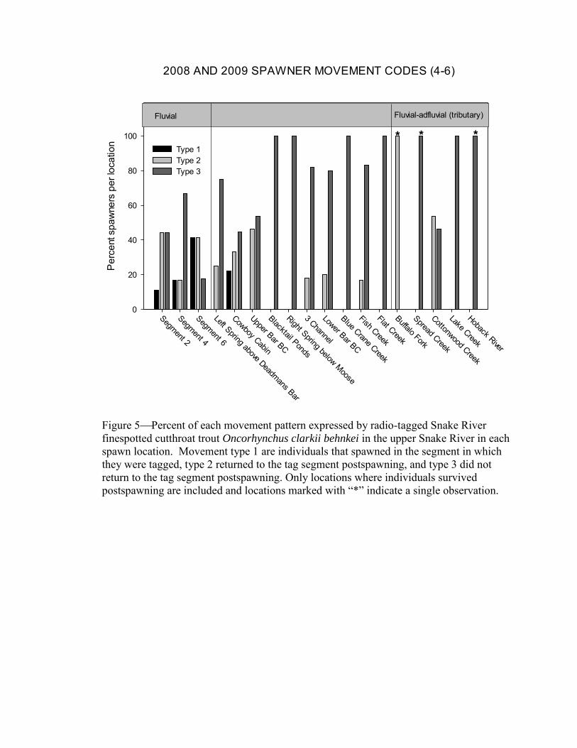
45
2008 AND 2009 SPAWNER MOVEMENT CODES (4-6)
Segment 2
Segment 4
Segment 6
Left Spring above Deadmans Bar
Cowboy Cabin
Upper Bar BC
Blacktail Ponds
Right Spring below Moose
3 Channel
Lower Bar BC
Blue Crane Creek
Fish Creek
Flat Creek
Buffalo Fork
Spread Creek
Cottonwood Creek
Lake Creek
Hoback River
Per
cent
spa
wne
rs p
er lo
catio
n
0
20
40
60
80
100Type 1Type 2Type 3
Fluvial Fluvial-adfluvial (tributary)
* * *
Figure 5Percent of each movement pattern expressed by radio-tagged Snake River finespotted cutthroat trout Oncorhynchus clarkii behnkei in the upper Snake River in each spawn location. Movement type 1 are individuals that spawned in the segment in which they were tagged, type 2 returned to the tag segment postspawning, and type 3 did not return to the tag segment postspawning. Only locations where individuals survived postspawning are included and locations marked with “*” indicate a single observation.
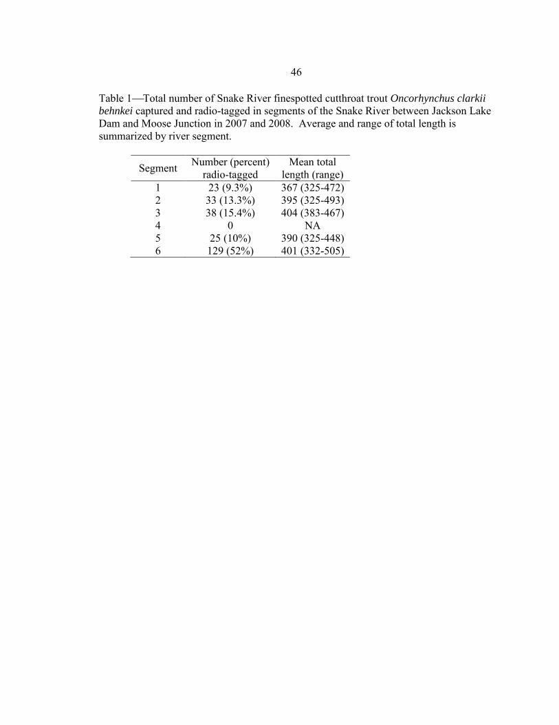
46 Table 1Total number of Snake River finespotted cutthroat trout Oncorhynchus clarkii
behnkei captured and radio-tagged in segments of the Snake River between Jackson Lake Dam and Moose Junction in 2007 and 2008. Average and range of total length is summarized by river segment.
Segment Number (percent) radio-tagged
Mean total length (range)
1 23 (9.3%) 367 (325-472) 2 33 (13.3%) 395 (325-493) 3 38 (15.4%) 404 (383-467) 4 0 NA 5 25 (10%) 390 (325-448) 6 129 (52%) 401 (332-505)

47
Table 2Spawning date, location, and habitat type (tributary, spring creek, or side channel) for 140 Snake River finespotted cutthroat trout Oncorhynchus clarki behnkei that made distinct spawning migrations in 2008 and/or 2009 in the upper Snake River watershed below Jackson Lake Dam. Springs designated as “left” or “right” are on river left or right.
Spawners Spawning Dates
Spawning Location 2008 2009 2008 2009 Spring Creeks 9 68 26 June – 21 July 14 May – 23 July 3 Channel 1 11 15 July 18 June - 8 July Blacktail Ponds 3 9 2 July - 9 July 16 June - 6 July Blue Crane Creek 4 5 June - 18 June Cowboy Cabin 1 8 26 June 14 May - 10 July Fish Creek 2 7 16 July - 21 July 18 May - 23 June Flat Creek 1 2 8 July 23 June Left Spring above Deadman’s Bar 3 4 June - 24 June Lower Bar BC 1 6 7 July 17 June - 9 July Right Spring below Moose 4 5 June - 12 July Upper Bar BC 14 17 June - 8 July Tributaries 9 19 14 June – 16 July 26 May – 28 July Buffalo Fork 4 26 May - 15 June Cottonwood Creek 3 11 17 June - 16 July 2 June - 28 July Ditch Creek 1 16 June Greys River 1 4 July Gros Ventre River 1 7 July Hoback River 1 14 July Lake Creek 2 5 June Pacific Creek 1 14-June Spread Creek 2 1 17 June – 14 July 24 June Snake River Side Channels 5 37 19 June – 17 July 27 May – 23 July Segment 2 10 28 May - 14 July Segment 4 1 5 17 July 4 June – 11 June Segment 6 4 22 19 June – 15 July 27 May – 23 July
47

48
References
Behnke, R. J. 1992. Native trout of western North America. American Fisheries Society Monograph 6.
Bennett, S. and J.L. Kershner. 2009. Levels of introgression in Westslope cutthroat
populations eight years after changes to rainbow trout stocking programs in southeastern British Columbia. North American Journal of Fisheries Management 29: 1271-1282.
Brenkman, S. J., G. R. Pess, C. E. Toregersen, K. K. Kloehnd, J. J. Dudae, and S. C.
Corbett. 2008. Predicting recolonization patterns and interactions between potamodromous and anadromous salmonids in response to dam removal in the Elwha River, Washington State, USA. Northwest Science 82(sp1): 91-106.
Carlson, A. J. and F. J. Rahel. 2010. Annual intrabasin movement and mortality of adult
Bonneville cutthroat trout among complementary riverine habitats. Transactions of the American Fisheries Society 139: 1360-1371.
Cole, L. C. 1954 The population consequences of life-history phenomena. The
Quarterly Review of Biology 29: 103-137. Colyer, W. T., J. L. Kershner, and R. H. Hilderbrand. 2005. Movements of fluvial
Bonneville cutthroat trout in the Thomas Fork of the Bear River, Idaho–Wyoming. North American Journal of Fisheries Management 25: 954-963.
Cowley, D. E. 2008. Estimating required habitat size for fish conservation in streams.
Aquatic Conservation: Marine and Freshwater Ecosystems 18: 418-431. DeRito, J. N., A. V. Zale, and B. B. Shepard. 2010. Temporal reproductive separation of
fluvial Yellowstone cutthroat trout from rainbow trout and hybrids in the Yellowstone River. North American Journal of Fisheries Management 30: 866-886.
Den Boer, P. J. 1968. Spreading of risk and stabilization of animal numbers. Acta
Biotheoretica 18: 165-194 Ebersole, J. L., W. J. Liss, and C. A. Frissell. 1997. Restoration of stream habitats in the
Western United States: restoration as reexpression of habitat capacity. Environmental Management 21: 1-14.
Fausch, K. D., C. E. Torgersen, C. V. Baxter, and H. W. Li. 2002. Landscapes to
riverscapes: bridging the gap between research and conservation of stream fishes. BioScience 52: 483-498.
49 Frissell, C. A., W. J. Liss, C. E. Warren, and M. D. Hurley. 1986. A hierarchical
classification for stream habitat classification: viewing streams in a watershed context. Environmental Management 10: 199-214
Greene, C. M., J. E. Hall, K. R. Guilbault, and T. P. Quinn. 2010. Improved viability of
populations with diverse life-history portfolios. Biology Letters 6: 382-386. Gregory, J. and S. Yates. 2009. Trout movement in the Gros Ventre River and access to
the Snake River. Final Draft Report produced by Gregory Aquatics for Trout Unlimited. September 2009.
Gresswell, R. E. and J. D. Varley. 1988. Effects of a century of human influence on the
cutthroat trout of Yellowstone Lake. American Fisheries Society Symposium 4: 45-52.
Gresswell R. E., W. J. Liss, and D. L. Larson. 1994. Life-history organization of
Yellowstone cutthroat trout (Oncorhynchus clarki bouvieri) in Yellowstone Lake. Canadian Journal of Fisheries and Aquatic Sciences 51 (Suppl. 1): 298-309.
Gresswell, R. E., W. J. Liss, G. L. Larson, and P. J. Bartlein. 1997. Influence of basin-
scale physical variables on life history characteristics of cutthroat trout in Yellowstone Lake. North American Journal of Fisheries Management 17: 1046-1064.
Gresswell, R. E. 1999. Fire and aquatic ecosystems in forested biomes of North
America. Transactions of the American Fisheries Society 128: 193-221. Gresswell, R. E. 2011. Biology, Status, and Management of the Yellowstone Cutthroat
Trout. North American Journal of Fisheries Management 31: 782-812. Gross, M. R. 1991. Salmon breeding behavior and life-history evolution in changing
environments. Ecology 72: 1180-1186. Harper, D. D. and A. M. Farag. 2004. Winter habitat use by cutthroat trout in the Snake
River near Jackson, Wyoming. Transactions of the American Fisheries Society 133: 15-25.
Hayden, P. S. 1967. The reproductive behavior of the Snake River cutthroat trout in
three tributary streams in Wyoming. Wyoming Game and Fish Commission, Cooperative Research Project 4. 105 pp.
Henderson, R., J. L. Kershner, and C. A. Toline. 2000. Timing and location of spawning
by nonnative rainbow trout and native cutthroat trout in the South Fork Snake

50
River, Idaho, with implications for hybridization. North American Journal of Fisheries Management 20: 584-96.
Hilderbrand, R. H. and Kershner, J. L., 2000a, Conserving inland cutthroat trout in small
streams: how much stream is enough? North American Journal of Fisheries Management, v. 20, p. 513-520.
Hilderbrand, R. H. and Kershner, J. L., 2000b, Movement patterns of stream-resident
cutthroat trout in Beaver Creek, Idaho-Utah: Transactions of the American Fisheries Society 129: 1160-1170.
Hilborn, R., T. P. Quinn, D. E. Schindler, and D. E. Rogers. 2003. Biocomplexity and
fisheries sustainability. Proceedings of the National Academy of Science 100: 6564-6568.
Hudy, M., B. Roper, and N. Gillespie. 2007. Large scale assessments: lessons learned for
native trout management. Proceedings of Wild Trout Symposium IX, West Yellowstone, MT, October 2007.
Joyce, M. P. and W. A. Hubert. 2004. Spawning ecology of finespotted Snake River
cutthroat trout in spring streams of the Salt River valley, Wyoming. Western North American Naturalist 64: 78-85.
Kaitala, A., V. Kaitala, and P. Lundberg. 1993. A theory of partial migration. The
American Naturalist 142: 59-81. Kiefling, J. W. 1978. Studies on the ecology of the Snake River cutthroat trout.
Wyoming Game and Fish Department, Fisheries Technical Bulletin 3. 198 pp. Knighton, D. 1998. Fluvial forms and processes. Oxford University Press, New York,
NY. Kovach, R, L. Eby, and M. P. Corsi. 2011. Hybridization between Yellowstone
cutthroat trout and rainbow trout in the upper Snake River basin, Wyoming. North American Journal of Fisheries Management 31: 1077-1087.
Marcus, W. A., R. A. Marston, C. R. Colvard Jr., and R. D. Gray. 2002. Mapping the
spatial and temporal distributions of woody debris in streams of the Greater Yellowstone Ecosystem, USA. Geomorphology 44: 323-335.
Marston R. A., J. D. Mills, D. R. Wrazien, B. Bassett, D.K. Splinter. 2005. Effects of
Jackson Lake Dam on the Snake River and its floodplain, Grand Teton National Park, Wyoming, USA. Geomorphology 71: 79-98.

51 Meka, J. M., E. E. Knudsen, D. C. Douglas, and R. B. Benter. 2003. Variable migratory
patterns of different adult rainbow trout life-history types in a Southwest Alaska watershed. Transactions of the American Fisheries Society 132: 717-732.
Miller, R. R., J. D. Williams, and J. E. Williams. 1989. Extinctions of North American
fishes during the last century. Fisheries 12: 22-38. Muhlfeld, C. C., T. E. McMahon, M. C. Boyer, and R. E. Gresswell. 2009. Local
habitat, watershed, and biotic factors influencing the spread of hybridization between native westslope cutthroat trout and introduced rainbow trout. Transactions of the American Fisheries Society 138: 1036-1051.
Nelson, M. L., T. E. McMahon, and R. F. Thurow. 2002. Decline of the migratory form
of bull charr Salvelinus confluentus, and implications for conservation. Environmental Biology of Fishes 64: 321-332.
Nelson, N. C. 2007. Hydrology and geomorphology of the Snake River in Grand Teton
National Park, Wyoming. Masters thesis, Utah State University, Logan, UT, 133 pgs.
Northcote, R. G. 1992. Migration and residency in stream salmonids-some ecological
considerations and evolutionary consequences. Nordic Journal of Freshwater Research 67: 5-17.
Northcote, R. G. 1997. Potamodromy in salmonidae living and moving in the fast lane.
North American Journal of Fisheries Management 17: 1029-1045. Novak, M. A., M. Binstadt, and E. K. Hall. 2004. Movement patterns of stream-resident
Snake River and Yellowstone cutthroat trout 2002-2004 radio telemetry project. Bridger-Teton National Forest.
Novak M. A., J. L. Kershner, and K. E. Mock. 2005. Molecular genetic investigation of
Yellowstone cutthroat trout and finespotted Snake River cutthroat trout. Wyoming Game and Fish Department report # 165/04.
Poff, N. L. and J. V. Ward. 1990. Physical habitat template of lotic systems: recovery in
the context of historical pattern of spatiotemporal heterogeneity. Environmental Management 14: 629-645.
Poff, N. L., J. D. Allan, M. B. Bain, J. R. Karr, K. L. Prestegaard, B. D. Richter, R. E.
Sparks, and J. C. Stromberg. 1997. The natural flow regime: a paradigm for river conservation and restoration. BioScience 47: 769-784.

52 Poole, G. C. 2002. Fluvial landscape ecology: addressing uniqueness within the river
discontinuum. Freshwater Biology 47: 641-660. Rieman, B. E. and J. D. McIntyre. 1993. Demographic and habitat requirements for
conservation of bull trout. General Technical Report INT-302. U.S. Forest Service, Intermountain Research Station, Ogden, UT.
Rieman, B. E., D. Lee, G. Chandler, and D. Myers. 1997. Does wildfire threaten
extinction for salmonids: responses of redband trout and bull trout following recent large fires on the Boise National Forest. Pages 47–57 in J. Greenlee, editor. Proceedings of the symposium on fire effects on threatened and endangered species and habitats. International Association of Wildland Fire, Fairfield, Washington.
Rieman, B. E. and J. B. Dunham. 2000. Metapopulations and salmonids: a synthesis of
life history patterns and empirical observations. Ecology of Freshwater Fish 9: 51–64.
Rieman, B., D. Lee, D. Brns, R. Gresswell, M. Young, R. Stowell, J. Rinne, and P.
Howell. 2003. Status of native fishes in the western United States and issues for fire and fuels management. Forest Ecology and Management 178: 197-211.
Rosgen, D. L. 1994. A classification of natural rivers. Catena 22:169-199. Ross, M. J. and C. F. Kleiner. 1982. Shielded-needle technique for surgically implanting
radio- frequency transmitters in fish. Progressive Fish Culturist 44: 41-43. Saiget, D. A., M. R. Sloat, and G. H. Reeves. 2007. Spawning and movement behavior
of migratory coastal cutthroat trout on the Western Copper River Delta, Alaska. North American Journal of Fisheries Management 27: 1029-1040.
Sanderson, T. B. and W. A. Hubert. 2009. Movements by adult cutthroat trout in a lotic
system: implications for watershed-scale management. Fisheries Management and Ecology 16: 329-336.
Schindler, D. E., R. Hilborn, B. Chasco, C. P. Boatright, T. P. Quinn, and L. A. Rogers.
2010. Population diversity and the portfolio effect in an exploited species. Nature 465: 609-612.
Schmetterling, D. A. 2001. Seasonal movements of fluvial westslope cutthroat trout in
the Blackfoot River drainage, Montana. North American Journal of Fisheries Management 21:507-520.

53 Schrank, A. J. and F. J. Rahel. 2004. Movement patterns in inland cutthroat trout:
management and conservation implications. Canadian Journal of Fisheries and Aquatic Sciences 61:1528-1537.
Sibly, R. M. 1991. The life-history approach to physical ecology. Functional Ecology 5: 184-191. Southwood, T. R. E. 1977. Habitat, the templet for ecological strategies. Journal of
Animal Ecology 46: 337-365. Southwood, T. R. E. 1988. Tactics, strategies, and templets. Oikos 52: 3-18. Starcevich, S. J. 2005. Seasonal movement patterns and habitat use of westslope cutthroat
trout in two headwater tributary streams of the John Day River. Master’s Thesis Oregon State University, Corvallis, Oregon.
Stearns, S. C. 1977. The evolution of life-history traits: a critique of the theory and a
review of the data. Annual Review of Ecology and Systematics 8:145-171. Stearns, S. C. 1989. Trade-offs in life-history evolution. Functional Ecology 3: 259-
268. Teuscher, D. M. and D. J. Schill. 2010. American white pelican predation on
Yellowstone cutthroat trout in the Blackfoot River system, Idaho in Carline, R.F., and C. LoSapio, editors. Conserving wild trout. Proceedings of the Wild Trout X symposium, Bozeman, Montana. 370 pages.
Thorp, J. H., M. C. Thoms, and M. D. Delong. 2006. The riverine ecosystem synthesis:
biocomplexity in river networks across space and time. River Research and Applications 22: 123-147.
Thurow, R. F., D. C. Lee, and B. E. Rieman. 1997. Distribution and status of seven
native salmonids in the interior Columbia River basin and portions of the Klamath River and Great Basins, North American Journal of Fisheries Management 17(4) 1094-1110.
Varley, J. D. and R. E. Gresswell. 1988. Ecology, status, and management of the
Yellowstone cutthroat trout. American Fisheries Society Symposium 4: 13-24. Warren C. E. and W. J. Liss. 1980. Adaptation to aquatic environments. Pages 15-40 in
R. T. Lackey, and L. Nielsen, editors. Fisheries Management. Oxford, UK: Blackwell Scientific Publications.

54 Wiens, J. A. 2002. Riverine landscapes: taking landscape ecology into the water.
Freshwater Biology 47: 501-515. Williams, J. E., A. L. Haak, H. M. Neville, and W. T. Coyler. 2009. Potential
consequences of climate change to persistence of cutthroat trout populations. North American Journal of Fisheries Management 29: 533-548.
Young, M. K. 1996. Summer movements and habitat use by Colorado River cutthroat
trout (Oncorhynchus clarki pleuriticus) in small, montane streams. Canadian Journal of Fisheries and Aquatic Sciences 53:1403-1408.

55
CHAPTER THREE
INTERPOLATING PROBABILISTIC MOVEMENT PATHS FROM SPARSE
TELEMETRY DATA IN A LINEAR SYSTEM
Abstract
Movement paths elucidate underlying processes and scales associated with
patterns of space-use (the continuous use of locations in the spatial dimension). In river
systems, technology and logistics limit collection of continuous fish movement data, and
resulting discrete data are often sparse. Sparse data may miss important ecological
features of fish movement and be biased toward over-representing use of locations where
fish are detected. Here, we address this issue with a new method for interpolating
movement paths from sparse relocation data collected at uneven sampling intervals. In
this adaptive kernel density interpolation (AKDI) method, a probabilistic distribution for
each time step is computed as a function of (1) the elapsed time to the temporally-nearest
relocation point, (2) the average velocity between consecutive relocations, and (3) the
degree of randomness in the movement. The AKDI method is compared with three
existing methods (sample data, fixed kernel density, and linear interpolation) in their
capacity to estimate a known utilization distribution. The AKDI method error rates are
significantly lower than the other three methods across a range of sample sizes.
Consequently, for real datasets, the AKDI method effectively generates movement paths
from sparse data as a precursor to better understanding space-use in river systems.

56
Introduction
Movement paths describe the continuous sequence of locations occupied by an
individual in the spatial domain during a defined temporal domain (Turchin 1998). The
spatial component of this path describes the pattern of space-use (i.e., the frequency of
use per location), whereas the temporal component describes the timing, direction, and
rate of movement between locations (Lucas and Baras 2000; Patterson et al. 2008). Both
components of the movement path are fundamental to describe the ecological link
between organisms and their environment and to investigations of how ecological
interactions and processes operate in space and time (Addicott et al. 1987; Turner et
al.1995; Keating and Cherry 2009). Moreover, movement paths are uniquely valuable
for elucidating the scales associated with hierarchical patterns of space-use (Johnson
1980; Wiens 1989; Pace 2001).
In stream systems, the capacity to identify movement paths is limited by
technology and logistics. As continuous GPS tracking signals do not travel through
water, movement paths must be determined from discrete tracking technology such as
radio telemetry (for multidirectional movement and assessments of habitat use), or fixed
antennae (for unidirectional movement past antennae when data on habitat use between
antennae is not needed). With radio telemetry, the frequency of relocations must be
balanced with spatial accuracy and sample size constraints (Garton et al. 2001; Hodder et
al. 2007). Consequently, data associated with discrete tracking are often sparse and may
produce misleading patterns of space-use. For example, discrete relocations of an
individual in a stream system may suggest areas of use and avoidance. However, given

57 that an individual is constrained to a continuous path, there should be no zero-probability
of space-use between locations where an individual was detected. Additionally, uneven
sampling intervals violate the implicit assumption that increased observations in a
location correspond to increased time spent in a location (Rogers and White 2007).
Finally, utilization distributions calculated from the density of relocation points (and not
temporally ordered points) may misrepresent the underlying movement path as the same
set of relocation points could be connected with different paths that each have unique
utilization distributions (Figure 1a and 1b). Given the potential biases of using discrete
sample data to understand space-use in stream systems, it may be preferable to interpolate
between sequential sample points to estimate a continuous movement path.
Numerous methods exist to interpolate movement paths, but each has specific
data requirements that are rarely met in telemetry datasets from stream systems.
Moreover, there are conceptual limitations that make existing methods unsuitable for
interpolating biologically meaningful movement paths. For example, if relocations are
represented as points in a space-time domain (X-t space), a linear interpolation between
these points will produce continuous movement paths even when data are sparse (Wentz
et al. 2003). However, interpolated values may be arbitrary because (1) the individual is
implicitly assumed to move at a constant velocity between relocations, and (2) the sample
frequency determines the perceived movement rate between locations. Time geography
(Downs 2010), Brownian bridges (Bullard 1999; Horne et al. 2007), and biased random
bridges (Benhamou 2011) estimate the probability that an individual will occur at a
specific distance from the last sample point as a function of a diffusion (or advection-

58 diffusion) rate, but these techniques have not been adapted for sparse data in one-
dimensional systems. Alternatively, kernel density techniques estimate a discontinuous
probability of use around sample points (Worton 1989; Manly et al. 2002; Vokoun 2003)
and account for error in telemetry relocations (Nams 1989). However, this approach is
sensitive to sample size and does not include the temporal component of space-use
(Rogers and White 2007).
In this paper, we describe a new method to generate a continuous probability field
of use across a spatiotemporal domain from sparse relocation data collected at variable
sampling intervals or during rapid migrations. Conceptually, this adaptive kernel density
interpolation method (AKDI) expands the concept of linear X-t interpolation by placing
an adaptive kernel over each point on the interpolation path to represent the probability of
time spent (and not density of relocation points) in the surrounding spatial domain. The
model takes the form of a piecewise advection-diffusion equation that captures both the
random (diffusive) and directed (advective) components of the movement path between
sample points, similar to the biased random bridge approach by Benhamou (2011).
However, the biased random bridge approach estimates three-dimensional space-use and
requires frequent relocation data and user-defined truncation of points that are too distant
from the interpolated path. In contrast, the AKDI approach applies the concept to a one-
dimensional physical space, for which a continuous probability field can be constructed
from sparse data with no arbitrary user inputs. The AKDI method is directly applicable
to stream systems where continuous data collection is precluded, but it could also be
applied to other one-dimensional systems such as wildlife corridors. Here we illustrate

59 the improved performance of the AKDI method relative to existing methods in estimating
a known movement path using sparse data.
Methods
The AKDI interpolation method was compared against raw data (naïve
distribution), linear interpolation, and fixed kernel density in their accuracy at
representing a “true” movement path with a utilization distribution. Simulated movement
paths were generated using a random walk algorithm and then randomly sampled to
provide a relocation dataset. Each method was applied to the relocation data without
knowledge of the “true” path or any user-defined input parameters, and the interpolated
paths were converted to utilization distributions. For each method, the difference
between the interpolated utilization distribution and the true utilization distribution were
calculated using root mean squared error (RMSE) for a uniform binning of the statistical
results. The process was repeated until the average error for a given number of
relocations converged for each method. (Supplement 1).
Adaptive Kernel Density Interpolation (AKDI) Method
The AKDI method estimates the probability that an individual was at a given
distance from a known relocation point after some elapsed time. Consider two
relocations whose coordinates are given by and . In a logically one-
dimensional (1-D) system, there exists a non-zero probability that the individual will pass
through all points internal to the observed locations during the time interval .

60 The average velocity over that time interval can be defined as
⁄ , which represents a linear path in space connecting the
relocations. The true behavior will deviate from this linear path, with the probable true
location becoming more uncertain with increasing time to the temporally-nearest
relocation point. Based on the probability of a 1-D biased random walk, we define a
continuously adaptive kernel density function, centered around the linear path, where the
probability at each point in the spatiotemporal domain is a function of the time ( and
distance to the temporally nearest relocation point, and characterized by a parameter
that represents degree of randomness in the motion:
√
This distribution is of the same form as the 1-D advection-diffusion equation,
where is analogous to the diffusion coefficient of the system. However, can be
determined solely from relocation data with no knowledge of the true motion and without
relying on user-specified parameters. For a given data set, the parameter can be
estimated by first defining a piecewise-linear interpolation path from the relocation data.
At a given point in time, the probability distribution around the linear path is a function
only of the two temporally-bounding relocation points. Therefore, at each relocation
point, the probability distribution can be computed based on a linear path directly
connecting the surrounding points to determine the value of that maximizes the
probability at the interior point. This is done for each point in the data set (except the
first and last), and the results are averaged to determine a value of that best represents
the system in an overall sense.

61
In practice the AKDI analysis is computed with the spatiotemporal domain
discretized into finite regions (bins) with modifications to avoid a singularity near the
relocation points as . The probability distribution is normalized at each point in
time allowing for finite spatial domains that may exist due to a physical barrier in the
system. Each time increment is equally weighted, and the results are averaged to
determine spatial distribution over a prescribed temporal domain; this provides an
intrinsic tolerance to uneven sampling frequencies.
Linear Interpolation
The linear interpolation method is a special case of AKDI with a zero-width
kernel, equivalent to estimating the distribution as that of a fish moving at a constant
velocity between relocation points. This method also has an intrinsic tolerance to
sampling frequency bias, and will converge as the number of samples increases, but it
does not account for the uncertainty inherent in a sparse dataset (Supplement 1).
Fixed Kernel Density
In the fixed kernel density method, a Gaussian probability field (kernel) was
calculated around each sample point (Supplement 1), and each sample point was evenly
weighted. As the choice of the kernel bandwidth may influence the resulting utilization
distribution (Silverman 1986), we used Silverman’s rule of thumb (SROT) to select the
optimal bandwidth and used the reduced factor of 0.9 to increase the probability that the
kernel would capture bimodality (Silverman 1986). This created a highly smoothed and

62 continuous probability of space-use that would be most comparable to the utilization
distributions calculated from the linear interpolation and AKDI methods.
Comparing Interpolation Methods
Simulated movement paths were created using a spatially 1-D random walk
algorithm in which the velocity and step size were randomly selected. (Supplement 1).
A single set of sample points was randomly selected from each random walk and used to
compute a utilization distribution with each of the interpolation methods (Appendix A).
This methodology avoided the biasing results based on the character (degree of
randomness) in a given dataset and provided a “true” path as a basis for quantitative error
analysis. (Appendix B). The utilization distribution of each interpolation method was
compared to the “true” utilization distribution by calculating root mean squared error
(RMSE; the difference in the frequency of use for each spatial bin in the domain). Test
runs were repeated until the RMSE for an approach at a given sample size converged.
Results
Interpolation methods were tested across sample sizes ranging from 5- 100 points
drawn from a random walk. With lower sampling efficiency, the domain of achievable
states around the interpolation path expands resulting in a more uniformly-distributed
space-use prediction, whereas high sampling efficiency leads to a narrow distributed
probability (Appendix B). The probability that an individual was at a given point in
space and time can be visualized as a 3-D surface across the spatiotemporal domain
(Figure 2). We note that while spatial extrapolation is allowed (either unbounded or with

63 some physical constraint such as a dam or waterfall) the temporal domain is limited to the
extents of the measured data.
The AKDI method was significantly better at estimating the space-use distribution
of the “true” movement path across sample sizes than the other three approaches (Figures
1 and 3). It is important to note that the “raw data” error is a function of the bin size and
should only be qualitatively compared to the other methods, which each generate a
continuous distribution. For example, at a sample size of 15, average RMSE was 8%,
11%, 16%, and 25% for AKDI, fixed kernel density, linear interpolation, and raw data,
respectively (Figure 3).
Discussion
In this paper, we described a new interpolation method that calculated a
continuous probability of time spent across the spatial domain of the data based on sparse
sample data. The AKDI method performed significantly better across sample sizes in
representing the “true” movement path than sample data, fixed kernel density, or linear
interpolation, while providing an intrinsic tolerance to uneven sampling frequency.
Irrespective of the interpolation method used, modeling results suggest that interpolated
movement paths better describe the underlying movement path than does raw sample
data. Only in the strict case where an individual migrates rapidly among discrete habitat
units would it be expected that sample point data would accurately represent space-use.
Thus, it appears that interpolation methods may represent a significant improvement over
existing techniques in describing patterns of space-use in a one dimensional system.

64
The AKDI method provided a better assessment of space-use because use was
calculated in terms of time spent in a location and accurately described positive values for
time spent across the spatiotemporal domain of the data. When the sample data were
sparse and unequally distributed across the spatial domain of the random walk, there were
areas of high and low densities of data collection (not necessarily corresponding to
differential densities in time spent; Rogers and White 2007). With sample data or fixed
kernel density, the areas of high sample point density were over emphasized, and little to
no probability of use was determined for areas of low density. In contrast, both the
AKDI and linear interpolation calculated space-use as a sample of time such that multiple
relocations in close temporal proximity counted for less time spent in that location than if
the same relocations had occurred further apart in time (Johnson et al. 2008a).
Conceptually, calculating use as the amount of time spent in a location improved
assessments of space-use when the sampling interval was uneven and was directly
analogous to point density estimates when the sampling interval was even.
The AKDI method was less sensitive to sample size than the other three methods
because it accounted for data sparseness by decreasing the probability of space-use for
interpolated points that were further from sample points. Both sample data and linear
interpolation did not capture the variability in space-use when based on small sample
sizes. However, if the true movement path were less random than the path tested here, it
is possible that linear interpolation would be sufficient to characterize the path (Wentz et
al. 2003). The performance of the kernel density estimator was also influenced by
sample size; at smaller sample sizes, the fixed kernel method performed slightly less well

65 than the AKDI method, particularly under conditions when the samples drawn from the
random walk were highly clustered. At larger sample sizes, the performance of the fixed
kernel method was more similar to the linear interpolation method due to the effect of
uneven sampling intervals. When using the SROT estimate for an optimal bandwidth
smoother, there is a balance between selecting a small enough factor value to capture
multimodality and selecting a large enough factor value to produce non-zero values
across the spatial domain of the data (Silverman 1986). The selection of this factor value
may be data-driven, but there is no clear “best” method for determining the bandwidth
value. Thus, although the RMSE of the kernel method may approximate the AKDI
method at small sample sizes, it is inherently based on arbitrary selection of a bandwidth.
More importantly, however, datasets based on actual movement patterns may not
conform to the random movements parameterized here. If the underlying utilization
distributions is more multimodal (e.g., for individuals that exhibit seasonal shifts in
habitat use), the fixed kernel method may perform more poorly, whereas the performance
of the AKDI method would be unaffected by the data distribution.
The AKDI method relies on the principle that information associated with
observed locations could inform estimates of use at intermediate locations because data
points within movement paths are serially autocorrelated (Manly et al. 2002). Other
researchers have used subsampling or aggregation techniques to create independence in
autocorrelated data (Johnson et al. 2008a). However, independence comes at the cost of
decreasing sample size and precision and of losing the context of the movement path or
behaviors that connect locations through time (de Solla et al. 1999; Nations and

66 Anderson-Sprecher 2006; Fieberg 2007; Johnson et al. 2008b). In contrast, space-time
movement paths retain the full sample size and the context of the movement path, and
thus represent an improvement in our understanding of space-use.
As presented, the AKDI method used equal-sized spatial bins for interpolation,
but unequal-sized bins could be used without modification to the method (complete code
for data processing provided in Supplement 2). This could be particularly useful if the
bin size were selected to correspond to hierarchical habitat features, which are generally
variable in length (Frissell et al. 1986). When combined with a spatial classification
system that is geomorphically-derived, the interpolated movement paths are even more
likely to capture those features of the physical template that influence movement rate
through a heterogeneous stream network (Johnson et al. 1992; Schippers et al. 1996).
The choice of spatial bin size in the interpolated path is limited to the smallest spatial
scale at which relocations are accurate because different movement patterns occur at
different spatiotemporal scales (Johnson 1980; Wiens 1989; Rettie and McLoughlin
1999). Likewise, interpolation only describes the time period (e.g., daylight hours) that
was sampled (Rettie and McLoughlin 1999).
This study highlighted the importance of using interpolated utilization distribution
data rather than raw sample point data to characterize space-use. Currently, most
telemetry studies in stream systems quantify relocation points in spatial units (e.g.,
reaches) to describe patterns of space-use, rather than analyze interpolated path data.
However, our modeling results suggest that under certain conditions (e.g., rapid, random,
or frequent movement), this approach may be significantly biased, perhaps to the point of

67 producing erroneous results. For example, in a 10-week telemetry study of fish
movement with weekly relocations, the average RMSE ≈ 30% for raw sample point data,
whereas the average RMSE would be < 10% for the AKDI method. In this case, the
sample point data may mischaracterize use of important habitat or corridors that would be
otherwise captured by the AKDI method.
In conclusion, the AKDI method can be used to identify a continuous probability
of space-use intermediate to sample points as a precursor to better understanding space-
use patterns in stream systems. Although data collection should not be reduced (as
important behavioral patterns may be missed), this method is quite useful for improving
our understanding of space-use when continuous data collection is precluded. It also
presents an array of opportunities to integrate sparse telemetry data sets into emerging
analytical frameworks (e.g., resource selection functions that use utilization distributions,
Millspaugh et al. 2006; or analyzing movement paths with state-space models, Jonsen et
al. 2003; Patterson et al. 2008) that require continuous data (Fieberg et al. 2010).
Acknowledgements
Michael Homel co-authored this paper and contributed to the statistical approach,
created and ran all code (Appendix B and Supplements 1 and 2), produced several
figures, and assisted with editing. Tom McMahon, Wyatt Cross, Jeff Kershner, and Kathi
Irvine reviewed previous drafts of this manuscript and provided valuable feedback.
Support was provided by the U.S. Geological Survey, Northern Rocky Mountain Science
Center, grant number: GX11RR0099I3400; the National Fish and Wildlife Foundation

68 One-fly, grant numbers: 2006-0095-007 and 2007-0074-010; the National Park Service,
grant number: F1460070060; and the University of Wyoming-National Park Service
research grant, grant number: DOINPS44175GRSW.

69
Figures
Figure 1.Two potential movement paths (A and B) connecting identical relocation points (panel A) with the corresponding patterns of space-use frequency generated from sample points contrasted against the actual utilization distribution of each movement path (panel B).

70
Figure 2.Interpolated probability of time spent along a continuous path through X (location)-t (time) space generated using the adaptive kernel density interpolation method (AKDI). The height of the plot corresponds to the probability of time spent in a particular location at a particular time.

71
Figure 3.Root mean square error of the adaptive kernel density interpolation method (AKDI), naive sample data, linear interpolation, and fixed kernel density across sample sizes ranging from 5 to 100.
Ro
ot
mea
n s
qu
are
erro
r (R
MSE
)
Number of relocations

72
References
Addicott, J. F., J. M. Aho, M. F. Antolin, D. K. Padilla, J. S. Richardson, and D. A. Soluk. 1987. Ecological neighborhoods: scaling environmental patterns. Oikos 49: 340-346.
Benhamou, S. 2011. Dynamic approach to space and habitat use based on biased
random bridges. Plos One 6: e14592. Bullard F. 1999. Estimating the home range of an animal: a Brownian bridge approach.
Thesis. University of North Carolina, Chapel Hill, North Carolina, USA. de Solla, S. R., R. Bonduriansky, and R. J. Brooks. 1999. Eliminating autocorrelation
reduces biological relevance of home range estimates. Journal of Animal Ecology 68: 221-234.
Downs, J. A. 2010. Time-geographic density estimation for moving point objects.
Lecture Notes in Computer Science 6292: 16-26. Fieberg, J. 2007. Kernel density estimators of home range use: smoothing and the
autocorrelation red herring. Ecology 88: 1059-1066. Fieberg, J., J. Matthiopoulos, M. Hebblewhite, M. S. Boyce, and J. L. Frair. 2010.
Correlation and studies of habitat selection: problem, red herring, or opportunity? Philosophical Transactions of the Royal Society B 365: 2233-2244.
Frissell, C. A., W. J. Liss, C. E. Warren, and M. D. Hurley. 1986. A hierarchical
framework for stream habitat classification: viewing streams in a watershed context. Environmental Management 10: 199-214.
Garton, E. O., M. J. Wisdom, F. A. Leban, and B. K. Johnson. 2001. Experimental
design for radiotelemetry studies. Pages 15-42 in J. J. Millspaugh and J. M. Marsluff, editors. Radio tracking and animal populations. Academic Press, San Diego, California, USA.
Hodder, K. H., J. E. G. Masters, W. R. C. Beaumont, R. E. Gozlan, A. C. Pinder, C. M.
Knight, and R. E. Kenward. 2007. Techniques for evaluating the spatial behaviour of river fish. Hydrobiologia 582: 257-269.
Horne, J. S., E. O. Garton, S. M. Krone, and J. S. Lewis. 2007. Analyzing animal
movements using Brownian bridges. Ecology 88: 2354-2363.

73 Johnson, D. H. 1980. The comparison of usage and availability measurements for
evaluating resource preference. Ecology 61: 65-71. Johnson, A. R., J. A. Wiens, B. T. Milne, and T. O. Crist. 1992. Animal movements and
population dynamics in heterogeneous landscapes. Landscape Ecology 7: 63-75. Johnson, D. S., J. M. London, M. Lea, and J. W. Durban. 2008a. Continuous-time
correlated random walk model for animal telemetry data. Ecology 89: 1208-1215.
Johnson D. S., D. L. Thomas, J. M. Ver Hoef, and A. Christ. 2008b. A general
framework for the analysis of animal resource selection from telemetry data. Biometrics 64: 968-976.
Jonsen, I. D., R. A. Myers, and J. M. Flemming. 2003. Meta-analysis of animal
movement using state-space models. Ecology 84: 3055-3063. Keating, K. A., and S. Cherry. 2009. Modeling utilization distributions in space and
time. Ecology 90: 1971-1980. Lucas, M. C. and E. Baras. 2000. Methods for studying the spatial behavior or
freshwater fishes in the natural environment. Fish and Fisheries 1: 283-316. Manly, B. F., L. McDonald, D. Thomas, T. McDonald, and W. Erickson. 2002.
Resource selection by animals: statistical design and analysis for field studies. Kluwer Academic Publishers, Boston, Massachusetts, USA.
Millspaugh, J. J., R. M. Nielson, L. McDonald, J. M. Marzluff, R. A. Gitzen, C. D.
Rittenhouse, M. W. Hubbard, and S. L. Sheriff. 2006. Analysis of resource selection using utilization distributions. The Journal of Wildlife Management 70: 384-395.
Nams, V. O. 1989. Effects of radiotelemetry error on sample size and bias when testing
for habitat selection. Canadian Journal of Zoology 67: 1631-1636. Nations, C., and R. Anderson-Sprecher. 2006. Estimation of animal location from radio
telemetry data with temporal dependencies. Journal of Agriculture, Biological, and Environmental Statistics 11: 87-105.
Pace, R. M. III. 2001. Estimating and visualizing movement paths from radio-tracking
data. Pages 189-206 in J. J. Millspaugh and J. M. Marsluff, editors. Radio tracking and animal populations. Academic Press, San Diego, California, USA.

74 Patterson, T. A., L. Thomas, C. Wilcox, O. Ovaskainen, and J. Matthiopoulos. State-
space models of individual animal movement. Trends in Ecology and Evolution 23: 87- 94.
Rettie, W. J. and P. D. McLoughlin. 1999. Overcoming radiotelemetry bias in habitat-
selection studies. Canadian Journal of Zoology 77: 1175-1184. Rogers, K. B., and G. C. White. 2007. Analysis of movement and habitat use from
telemetry data in C. S. Guy and M. L. Brown, editors. Analysis and interpretation of freshwater fisheries data. American Fisheries Society, Bethesda, Maryland, USA.
Schippers, P., J. Verboom, J. P. Knaapen, and R. C. van Apeldoorn. 1996. Dispersal and
habitat connectivity in complex heterogeneous landscapes: an analysis with a GIS-based random walk model. Ecography 19: 97-106.
Seaman, D. E., J. J. Millspaugh, B. J. Kernohan, G. C. Brundige, K. J. Raedeke, and R.
A. Gitzen. 1999. Effects of sample size on kernel home range estimates. Journal of Wildlife Management 63: 739-747.
Silverman, B. W. 1986. Density estimation for statistics and data analysis. Chapman
and Hall, London. Turchin, P. 1998. Quantitative analysis of movement. Sinauer Associates, Sunderland,
Massachusetts, USA. Turner, M.G., R. H. Gardner, and R. V. O’Neill. 1995. Ecological dynamics at broad
scales. BioScience, 1995(Suppl.): S29–S35. Vokoun, J. C. 2003. Kernel density estimates of linear home ranges for stream fishes:
advantages and data requirements. North American Journal of Fisheries Management 23: 1020-1029.
Wentz, E. A., A. F. Campbell, and R. Houston. 2003. A comparison of two methods to
create tracks of moving objects: linear weighted distance and constrained random walk. International Journal of Geographical Information Science 17: 623-645.
Wiens, J. A. 1989. Spatial scaling in ecology. Functional Ecology 3: 385-397. Worton, B. J. 1989. Kernel methods for estimating the utilization distribution in home-
range studies. Ecology 70: 164-168.

75
CHAPTER FOUR
SCALING UP: SPATIAL AND HIERARCHICAL VARIATION IN MOVEMENT
AND HABITAT OCCUPANCY PATTERNS
OF CUTTHROAT TROUT IN THE
UPPER SNAKE RIVER, WY
Abstract
Numerous salmonid habitat studies have described how habitat is hierarchically
structured, with physical characteristics at coarser spatiotemporal scales constraining the
expression of characteristics at finer scales. However, over longer spatial extents,
longitudinal and patchy variation in the physical template also affect habitat availability.
In particular, physical characteristics differ substantially among segments of stream
bounded by tributary junctions or pronounced changes in underlying geology, and it is
difficult to investigate habitat relationships that extend across multiple segments. To
date, most habitat and movement studies have focused on smaller streams and finer
spatial scales, and it is unclear whether relationships observed in smaller systems can
“scale up” in 4th-6th order river systems. In this study, radio-telemetry was used to
evaluate nonreproductive movement patterns and spatial variation in habitat occupancy of
Snake River finespotted cutthroat trout Oncorhynchus clarkii behnkei (n = 94) at two
spatial scales in the upper Snake River. Habitat availability and occupancy differed
substantially throughout the study area; one sample reach was associated with 24% of
occupancy, whereas several others were rarely occupied. In general, more time was spent

76 in reaches with a greater abundance of large woody debris and a greater maximum depth.
However, in the reaches immediately below Jackson Lake Dam, a stronger relationship
existed with submerged macrophytes. Habitat relationships were consistent throughout
the year because individuals exhibited little movement (primarily among adjacent
reaches). These data suggest that longitudinal and patchy variation in the physical
template, along with hierarchical habitat structure, produced variation in the spatial
availability of habitat attributes and occupancy. By evaluating habitat occupancy and
movement over a large spatial extent (45 km), with a large sample size of radio-tagged
cutthroat trout, and with data collected in great detail over multiple years, this study
addressed a data gap in our understanding of how cutthroat trout respond to habitat in
larger rivers.
Introduction
Salmonids connect seasonal (Fretwell 1972; Schlosser and Angermeier 1995;
Northcote 1997) or life-stage specific (Schlosser 1991) habitats with movement to
complete the life cycle (Schlosser 1991). Movement distance is a function of the
differential availability (Albanese et al. 2004), quality (Albanese et al. 2004), and spatial
arrangement (Kocik and Ferreri 1998; Bahr and Shrimpton 2004) of habitat (Carlson and
Rahel 2010). However, unique physical processes structure habitat across spatiotemporal
scales (Wiens 1989; Bult et al. 1998; Lowe et al. 2006), and it may be difficult to identify
important habitat relationships and associated movement scales across streams or stream
sizes.

77
Hierarchical structure in the physical template produces scale-specific habitat
relationships (Bozek and Rahel 1991; Rabeni and Sowa 1996; Bult et al. 1998).
Geomorphic features of the physical template are delineated according to a set of criteria
related to channel form and the frequency of channel reorganization (Frissell et al. 1986).
These features are nested hierarchically such that coarse-scale physical attributes
constrain the expression of fine-scale physical attributes (Frissell et al. 1986; Townsend
1996; Poole 2002). As a result, different habitat relationships may be associated with
particular scales in the hierarchy. For example, bull trout have been shown to select redd
sites in complex habitat characterized by upwelling groundwater at the reach scale, yet
downwelling flow at the microhabitat (redd-site) scale (Baxter and Hauer 2000).
Although habitat relationships are associated with different scales (Rabeni and Sowa
1996), spatial variation in the physical template affects the specific habitat availability or
relationships that can exist throughout a river network.
Habitat availability, occupancy, and movement patterns vary spatially in response
to habitat patchiness (Pringle et al. 1988) and longitudinal change (Vannote et al. 1980)
in the physical template. First, spatial variation among habitat at a given scale (e.g.,
variation among reaches) produces a patchy riverscape (Pringle et al. 1988; Poole 2002;
Thorp et al. 2006). For example, sediment erosion, transport, and deposition vary
spatially (Montgomery and Buffington 1997) and affect channel form (Montgomery and
Buffington 1997) and habitat availability. Thus, spatial variation in habitat availability
may result from underlying geology. This patchiness (or discontinuum; Poole 2002) may
be more pronounced at the segment scale, where segment breaks are defined by tributary

78 junctions or pronounced changes in geomorphology or geology that persist at intervals
greater than 100 years (Frissell et al. 1986; Ward and Stanford 1983).
In longer sections of streams, longitudinal changes to the physical template result
from increasing drainage area, spatial variability of the hydrograph (Vannote et al. 1980;
Gomi et al. 2002), disturbance regime (Montgomery 1999; Gomi et al. 2002), decreasing
elevation, and increasing temperature (Isaak and Hubert 2001). As such, the physical
attributes of reaches in a headwater stream may be dissimilar from attributes of reaches
lower down in the river (Gomi et al 2002). Moreover, in larger systems, fewer tributary
confluences are large enough relative to the main stem to impart a geomorphic effect
(Benda et al. 2004) or act as a segment boundary, and therefore, downstream segments
are often much longer than upstream segments. Thus, coarse, longitudinal change in
habitat-forming processes (e.g., temperature associated with elevation) influences the
attributes of individual reaches or segments spatially (Poff and Ward 1990; Montgomery
and Buffington 1997; Torgersen et al. 2006).
Collectively, hierarchical habitat structure, habitat patchiness, and longitudinal
changes to the physical template interact to define the set of habitat attributes available in
a particular location (Poole 2002; Benda et al. 2004). For example, different locations
are associated with different underlying geology, land use, discharge regime (Gomi et al.
2002), temperature regime, drainage pattern (Benda et al. 2004), or substrate size
(Schlosser 1991). Consequently, different habitat forming processes (e.g., sediment
transport) and habitat attributes (e.g., undercut banks) are distributed spatially throughout
the riverscape (Montgomery and Buffington 1997), and location within the riverscape

79 sets the context of how individuals use a system (Fausch et al. 2002; Weins 2002;
Carlson and Rahel 2010).
Recently, there has been a greater emphasis on riverscape-scale studies in stream
systems (Carbonneau et al. 2011; Brenkman et al. 2012; Thorp et al. 2013) as a way to
relate spatiotemporal variability in the physical template to salmonid habitat occupancy
or movement. However, most of the data on habitat occupancy or movement patterns
comes from smaller streams or finer spatial scales. Considering the substantial variation
in disturbance regimes and physical characteristics associated with stream size and
habitat scale, it is unlikely that patterns observed in smaller systems or finer scales can
“scale up” to describe patterns in larger systems or coarser scales. Consequently, there is
a need to explicitly evaluate spatial patterns of habitat occupancy and movement in 4th –
6th order rivers at the segment scale at which many trout complete their life cycle (Fausch
et al. 2002).
In this study, we evaluated spatial variation in habitat relationships and movement
patterns at the reach and segment scales, with emphasis on identifying spatial variation in
habitat relationships. Snake River finespotted cutthroat trout Oncorhynchus clarkii
behnkei in the upper Snake River provided a model system to explore habitat occupancy
and movement patterns. This subspecies persists throughout the native range in the upper
Snake River between Jackson Lake Dam and Palisades Reservoir. Much of the range in
the headwaters of Pacific Creek and Buffalo Fork was declared wild and scenic in the
Craig Thomas Snake River Headwaters Legacy Act of 2008. Because of the size of the
river system, cutthroat trout have the potential to make long-distance movements to

80 access seasonal habitat in a complex physical template (Sanderson and Hubert 2009;
Homel et al. in prep-a).
To better understand spatial habitat relationships, radio telemetry was used to
identify movement and habitat use by Snake River finespotted cutthroat trout in the upper
Snake River. Our specific objectives were (1) to identify the spatiotemporal scales
associated with nonreproductive movement patterns of cutthroat trout in the Snake River,
and (2) to evaluate spatial and hierarchical habitat relationships of adult cutthroat trout in
the Snake River. Previous research had identified complex movement patterns by adult
cutthroat trout throughout the year spawning occurs (Homel et al. in prep-a). To remove
potential bias in habitat occupancy that could result from a spawning migration, analysis
was restricted to adult cutthroat trout for which a spawning migration was not detected
during the study.
Methods
Research on the movement patterns and habitat occupancy of cutthroat trout
occurred in the upper Snake River in Grand Teton National Park between Jackson Lake
Dam and Moose Junction (45 km downstream of the dam; Figure 1). Jackson Lake Dam
was constructed at the outflow to Jackson Lake in 1906 to provide flood control and
irrigation water, which resulted in a modified discharge regime (Nelson 2007).
Following the construction of Palisades Dam (110 km below Jackson Lake Dam) in
1958, peak discharge released from Jackson Lake Dam has been more consistently timed
with natural runoff (mean = 182 m3/s at Jackson Lake Dam and 352 m3/s at Moose

81 Junction; Nelson 2007), and minimum winter discharge has been released (≥ 7.9 m3/s;
Nelson 2007). However, above average discharge is released from the dam during July,
August, and September for recreation activities on the Snake River and to maintain
sufficient irrigation water in Palisades Reservoir. At the confluence with Pacific Creek
and Buffalo Fork, 8 km below Jackson Lake Dam, the effects of discharge regulation
(sediment deficit, limited large woody debris, and altered hydrology; Marcus et al. 2002;
Marston et al. 2005; Nelson 2007) are mitigated by these two major tributaries.
Within the study area, sample segments and reaches were delineated according to
geomorphic characteristics (Frissell et al 1986). Segment breaks were established at
tributary junctions or where major geologic features (e.g., alluvial fan) exerted a
geomorphic control over a large section of river. Reaches were classified based on
channel constraint and channel morphology (i.e., single, multiple, or braided channels).
Cutthroat trout were implanted with radio tags in 2007 (n = 49) and 2008 (n =
199). Radio tagging effort was allocated spatially in proportion to the density of fish
observed during raft-electrofishing surveys conducted with Wyoming Game and Fish in
October (see Homel et al. in prep-a for a detailed description of radio-tagging methods).
All adult cutthroat trout > 325 mm (total length; TL) were implanted with a Lotek
Wireless radio-tag using a modified shielded needle technique (Ross and Kleiner 1982).
A total of 13 radio frequencies were used with approximately 19 fish per frequency. At
each frequency, unique burst patterns differentiated individual fish. Four tag sizes were
used (Lotek Wireless MCFT series: 3EM, 3FM, 3A, and 3L) to maximize the size range
of cutthroat trout that could be tagged without the tag weight exceeding 3% of the body

82 weight. Burst rates were programmed at 3-5 seconds to decrease the amount of signal
collision that could happen in a small study area with a large number of tagged fish.
Estimated tag battery life ranged from 334 days for the smallest tags (3EM) to 1,100 days
for the largest tags (3L).
From the initial sample size of 248 cutthroat trout, only those cutthroat trout that
were not detecting making distinct spawning migrations and were relocated at least two
times were considered non-spawning cutthroat trout with sufficient data for analysis.
Spawning migrations were defined in Homel et al. (in prep(a)) as rapid, directed
migrations between April and July. Cutthroat trout tagged in 2007 were relocated
bimonthly November-January and weekly April- November. Cutthroat trout tagged in
2008 were relocated bimonthly November- January, weekly May-July, and biweekly
August- October. Relocations were obtained by hiking, rafting, driving, and biking with
an antenna through the study area. Additional relocation data were obtained from
telemetry flights using a fixed wing aircraft with 4-element Yagi antennae, and attempts
were made to obtain a second ground relocation for these cutthroat trout within a week of
the telemetry flight.
Relocation data for each individual provided an observed location at a point in
time. However, some individuals were not encountered every week, and observed
locations did not necessarily indicate an individual was “using” the habitat where it was
encountered. Moreover, locations between where fish were observed were known to
have been occupied for some amount of time, but there was uncertainty in the estimate of
time spent in those locations. Therefore, it was necessary to interpolate between

83 observed relocation points and represent location uncertainty with utilization distributions
(an estimate of time spent per week in each reach). The adaptive kernel density
interpolation method (AKDI; Homel et al. in prep-b) was used to estimate utilization
distributions for each individual for the duration that the individual was alive and actively
tracked. These utilization distributions encompassed the probable range of reaches that
could be occupied by an individual during each week, given an observed movement rate
before and after that week. Practically, these utilization distributions represented an
estimate of reach occupancy for each time step; the term ‘reach occupancy’ will be used
hereafter to describe the probable time spent in each reach, for each week.
Spatiotemporal Movement Patterns
Movement paths were assembled from the dataset of weekly reach occupancy.
For each week, the description of reach occupancy was reduced to the single reach in
which the majority of time was spent. Each of these weekly maximum values was
aggregated into a set of consecutive locations through time that comprised a movement
path.
Spatiotemporal movement patterns (movement distance and percent of individuals
moving) were identified at the reach and segment scales from October 2007 through
September 2009 for each month, season, and year of the study. Seasons were defined by
the hydrograph as base flow (October 1-April 14), runoff (April 15-July 31), and elevated
summer flow (August 1-September 30; Figure 2). Movement distance was calculated as
the difference (in reaches or segments) between the most upstream and downstream reach
or segment occupied by an individual during each month. Monthly movement distance

84 was aggregated at seasonal and annual scales. The percent of individuals moving was
calculated based on the total number of living fish during a time step. Individuals were
considered to be moving if a single change in location at the reach or segment scale
occurred during the time interval (e.g., month). To facilitate comparisons across time
intervals, distance moved per time interval and percent fish moving per time interval
were standardized by the number of days in the time interval (e.g., season length).
Habitat Relationships
Prior to evaluating habitat relationships, reach occupancy data were transformed
to the appropriate temporal scale for analysis. First, weekly estimates of reach occupancy
were aggregated to create monthly estimates of reach occupancy, which were then
standardized by the duration of each month. Because the focus of this study was to
evaluate habitat patterns and not to predict individual relationships, monthly estimates of
reach occupancy were summed across individuals to produce a single monthly estimate
of reach occupancy for all fish, combined. Next, many of the monthly estimates of reach
occupancy were expected to be similar due to limited movement at certain times of the
year. Therefore, principle components analysis (PCA) was used to reduce the number of
months in the dataset (rows = reaches, columns = monthly occupancy) by identifying
clusters of months with similar estimates of reach occupancy (R, package labdsv, version
1.5-0; Roberts 2012). Similar clusters were subsequently aggregated to reduce the total
number of monthly reach occupancy analyses that were performed.
For each reach, habitat attributes were delineated according to the channel form in
2009 (corresponding to the time frame when radio-tagged cutthroat trout were tracked,

85 habitat attributes were measured, and current aerial photographs were available to derive
GIS habitat attributes for the habitat analysis; Table 1). Habitat attributes were selected
that were frequently cited as important habitat for cutthroat trout either individually (e.g.,
large woody debris, Young 1996; Kershner et al. 1997; and pools, Harper and Farag
2004; Sanderson and Hubert 2009) or as components of habitat complexity (braid index
and channel form; Horan et al. 2000). In addition, macrophytes and bank structure were
selected because they were common in different portions of the upper Snake River and
could be important sources of habitat complexity (Table 1).
The relationship between spatial patterns of reach occupancy and habitat
attributes was evaluated using multiple regression (R, package nlme, version 3.1-106;
Pinheiro et al. 2012). Specifically, regression was used to (1) identify the relationship
between reach occupancy and physical attributes throughout the study area, (2)
determine whether differences in the physical characteristics between segment 1 (the
upper most, regulated segment below Jackson Lake Dam) and the remaining five
segments (downstream of large tributary inputs), resulted in different reach-scale habitat
relationships, and (3) determine whether segment-scale attributes produced different
reach-scale attributes throughout the study area.
To address the first two objectives, regression models were fit to three datasets: a
full dataset of all reaches, a dataset of only the reaches in segment 1, and a dataset of all
reaches from segments 2 - 6. To address the third objective, mixed effects models were
constructed for the full dataset and the segments 2-6 dataset with segments modeled as a
random grouping variable to test whether relationships between reach occupancy and

86 habitat attributes varied systematically due to segment-level characteristics. Models were
constructed using the following formula:
( ) ( )
where is the total amount of time spent per location across all individuals is the
common intercept, is the between-group error term, is the slope of the first
predictor ( ), and is the within-group error term. Fixed effects models were
constructed for the segment 1 dataset (because there was no grouping variable) using the
following formula:
( ) ( )
where is the total amount of time spent per location across all individuals, is the
slope of the first predictor ( ), and is the error term.
For the full and segment 2-6 datasets, the same a priori candidate models were
constructed. For the segment 1 dataset, attributes used in the candidate models were
evaluated individually because the sample size precluded more complex model
constructions. In order to minimize the potential for multicollinearity in the model, a
correlation matrix (Table 2) was constructed for all predictor variables (Table 1). For
pairs of variables that were strongly correlated (r > 0.7), only the variable that was more
strongly correlated with reach occupancy was retained in the dataset. From that reduced
dataset, variables that were moderately correlated (r = 0.5 - 0.7) were not combined in
candidate models, but were used in independent models.
Models in the full and segment 2-6 datasets were contrasted using AIC scores to
show relative difference from the global model; scores differing by two or more points

87 (for models containing only significant variables) were considered to be significantly
different (Burnham and Anderson 1998). The variance explained by the random
intercept in each model (group level differences among segments) was calculated as
intercept variance/ (intercept + residual variance). Models in the segment 1 dataset were
not nested, so comparisons among significant models were ranked by the r2 value.
Results
A total of 6 segments (length = 4.9 – 11.7 km, mean = 7.2 km) and 32 reaches
(length = 0.3 – 4.9 km, mean = 1.4 km) were delineated in the Snake River between
Jackson Lake Dam and Moose Junction (Figure 1; Table 2). In segment 1 (below
Jackson Lake Dam), the channel is constrained with deep bedrock pools, and the
hydrograph is dominated entirely by releases from Jackson Lake dam. In contrast,
segments 2-6 have more complex habitat and substantially more gravel and large woody
debris, due to inputs from Pacific Creek and Buffalo Fork (Marcus et al. 2002; Marston et
al. 2005; Nelson 2007; Table 2). However, segment 4 is constrained by alluvial deposits
and has simpler habitat than upstream and downstream segments (Table 2).
A total of 94 cutthroat trout (mean length = 394 mm TL, range = 325 - 505) were
considered to be nonspawners based on a lack of directed movement to known spawning
areas between April and July when spawners were moving (Homel et al. in prep- a). Of
these 94 cutthroat trout, 19 were tagged in 2007 and relocated an average of 16.4 times
(range =2 - 42 relocations) from October 2007 to September 2009. The 75 cutthroat trout

88 tagged in 2008 were relocated an average of 12.6 times (range = 2 - 30 relocations) from
October 2008 to September 2009.
Spatiotemporal Movement Patterns
During all months, approximately 10% of individuals were moving at the reach
scale, but up to 45% moved during November, February, and May in 2007 and 2008
(Figure 3). At the segment scale, approximately 10 - 30% of individuals were moving
during all months except June-August in 2007, when only 5% of individuals were
moving; most segment-scale movement occurred during October, February, April, and
May (Figure 3). Likewise, most seasonal movement occurred during base flow and
runoff in 2007 and 2008, and substantially fewer individuals moved during the post-
runoff season (< 40% at the reach scale and < 20% at the segment scale; Figure 4).
Although the majority of individuals moved among reaches or segments at least
once during the year, monthly movement distances were very short (of those individuals
that moved, median = 2 reaches and 1 segment) in 2007 and 2008. Seasonal reach-scale
movement distances were also very short in 2007 (median = 2 reaches and 2 segments in
all seasons), and 2008 (base flow median =3 reaches and 1 segment, runoff median = 5
reaches and 2 segments, and post-runoff median =4 reaches and 1 segment). Annual
reach-scale movement distances (sum of monthly movement distances in 2007 and 2008)
were more pronounced; 62 individuals (66%) moved > 5 reaches (median = 8; Figure 5)
and 52 individuals (55%) moved > 1 segment (median = 3; Figure 6).

89 Habitat Relationships
Physical attributes of reaches and reach occupancy differed within and among
segments throughout the study area (Table 2). Large woody debris was extremely
abundant in segment 6, whereas macrophytes were abundant in segment 1 (Table 2).
Deep water was found throughout the study area, but the deepest channels were in
segment 1 (Table 2). Vertical or undercut banks were common in segment 2, 4, and 6
(Table 2). Overall, different types of complex habitat were available spatially, and most
reaches contained multiple types of complex habitat (e.g., braided channels and undercut
banks both common in the reaches of segments 2 and 6). Following the pattern of where
complex habitat was located, reach occupancy was highest in segments 1, 2, and 6, with
41% of occupancy in reaches 29, 31, and 32 of segment 6 (Figure 1, Table 2).
Although limited movement was detected among reaches during all time steps,
movement did not result in a change in reach occupancy (Figure 7). Variation in
occupancy among reaches was greater than variation in reach occupancy among months
(Figure 8); the first component of the PCA explained 99% of the variation, and all
reaches were loaded equally onto that component (Figure 8). Equal loading of reaches
suggests that the component was associated with variation in reach occupancy among
reaches, but not variation in occupancy among months. Accordingly, all monthly
estimates of reach occupancy were summed into a single, annual estimate of reach
occupancy, which was used as the response variable in the habitat analysis.
Many of the environmental predictor variables were correlated (Table 3), and
from an initial dataset of 11 variables (Table 1), 8 were retained in candidate models. For

90 the full dataset and the segment 1 dataset, a square root transformation was required for
reach occupancy and two of the predictor variables (thalweg length and large woody
debris) in order to normalize the residuals and achieve homoscedasticity. For the
segment 2-6 dataset, a log transformation was required for those same variables.
Accordingly, 10 mixed-effects models were constructed for each dataset (Table 4) with a
random intercept for each segment.
Top models varied among analyzed datasets. For the full dataset, the top model
predicted reach occupancy as a function of large woody debris and maximum depth
(Table 5), with segment modeled as a random intercept. No other models were within
two AIC points (Table 5). For the segments 2 - 6 dataset, the top model predicted reach
occupancy as a function of large woody debris and maximum depth (Table 5), identical
to the top model for the full dataset. For the segment 1 dataset, only single variable, fixed
effects models were fit because of the decreased sample size (n = 7 reaches; Table 4).
For this dataset, the best predictor of reach occupancy was the length of the channel
dominated by submerged macrophytes (Table 5).
Discussion
This study provided new information on habitat relationships and movement
scales by cutthroat trout in an intermediate-sized river. By collecting detailed habitat and
movement data over a large spatial extent (45 km), for multiple years, and with a large
sample size of radio-tagged cutthroat trout (n = 94), movement and reach occupancy
patterns could be detected at a level of detail not previously described. Nonspawning

91 adults exhibited limited movement among reaches, but movements were still longer than
those typically observed in headwater streams because reach length increases with stream
size. Thus, movement distance appeared to increase from headwater streams to larger
rivers, but movement scale (movement at the reach scale) did not. Analysis of occupancy
data demonstrated that spatial variation in habitat availability and habitat forming
processes among segments produced unique reach-scale habitat relationships throughout
the study area. These patterns were not analogous to those seen in headwater streams,
where salmonids occupy shorter extents of the stream (Heggenes et al. 1991; Petty et al.
2012) and encounter less longitudinal variation in habitat. As conservation efforts
increase in larger river networks, it will be important to consider contextual habitat
relationships that span stream sizes associated with different disturbance regimes (Gomi
et al. 2002) and habitat attributes.
In the upper Snake River, movements among reaches and segments were more
frequent during times of rapidly changing discharge (October), base flow, or spring
runoff, but distances were typically short (< 5 reaches or 1 segment). This seasonal
movement is similar to what has been seen in smaller systems, where short, channel unit-
scale movements are more common throughout the year, and longer reach and segment-
scale movements occur during periods of elevated discharge (Young 1996; Gresswell and
Hendricks 2007). With such limited movement by nonspawners, movement patterns did
not support the generalization that trout in larger systems move much longer distances
(Schrank and Rahel 2004; Zurstadt and Stephan 2004; Colyer et al. 2005) and have much
larger home ranges (Colyer et al. 2005; Schoby and Keeley 2011) than in headwater

92 systems. Although long spawning migrations were observed in this system (Homel et al.
in prep-a), it appears that nonspawners occupying a high-quality stream have little need
to move. Overall, movement among reaches indicated that habitat availability or quality
differed among reaches, and infrequent movement among segments implied that
segments contained the seasonal diversity of habitat required by nonspawning adult
cutthroat trout.
Reach occupancy was positively associated with complex habitat, however
different attributes comprised that complexity. In the Full and Segment 2-6 models,
reach occupancy was positively associated with large woody debris and maximum depth
of the reach. Large woody debris (Young 1996; Kershner et al. 1997) and pools (Dare
and Hubert 2003; Harper and Farag 2004; Sanderson and Hubert 2009) are frequently
identified as habitat for cutthroat trout, yet in the Snake River, these features were much
larger than may be seen in smaller systems. For example, in a small stream, pieces of
wood 1 m long and 10 cm in diameter may function as large woody debris (Kershner et
al. 2004). In the upper Snake River, whole trees or log jams functioned as large woody
debris, resulting in gravel deposition and formation of complex channels (Abbe and
Montgomery 1999). Likewise, pools in this system ranged from 10s of meters to over a
kilometer in length, consistent with the pattern that pool depth increases with increasing
stream size (Carlson and Rahel 2010). However, deep water was more often associated
with runs or glides, than actual pools. Finally, in the Segment 1 model, macrophytes
were positively associated with occupancy. Macrophytes have been shown to function as
complex habitat in the Henry’s Fork of the Snake River (Van Kirk and Martin 2000) and

93 were encountered in quasi-lentic reaches in the upper Snake River. Overall, although
habitat relationships appeared to be a scaled-up version of what is seen in smaller streams
based on the increased size of habitat attributes, spatial analysis of occupancy revealed
strong contextual variation within and among stream segments.
Spatial variation in habitat relationships was produced by longitudinal increases in
stream size. Longitudinal changes from major tributary inputs were pronounced between
segments 1 and 2. Above the tributaries, cutthroat trout were associated with complex
habitat in low gradient habitat. Below the tributaries, the geomorphic characteristics of
the Snake River changed substantially because of increased discharge and increased
delivery of sediment and large woody debris (Marcus et al. 2002; Marston et al. 2005;
Nelson 2007). Here, cutthroat trout were associated with large woody debris and reaches
with a greater maximum depth.
Segment-scale constraints on reach habitat also produced habitat patchiness and
contextual variation in occupancy. In segment 5, for example, the channel was
constrained by alluvial deposits and the gradient and water velocity increased
dramatically relative to upstream and downstream segments. Despite the availability of
velocity refugia (boulders and large woody debris), individuals spent very little time in
this segment. Likewise, the channel form in segment 4 was very complex, but with little
wood in the reach, occupancy was low. Thus, the combination of longitudinal, patchy,
and hierarchical variation in the physical template produced spatial variation in habitat
availability and habitat relationships.
Because particular reaches were occupied substantially more often than others,

94 perceived habitat relationships in the Full model were driven by the relationships found
in high occupancy reaches. In particular, reaches 29, 31, and 32 were associated with
40% of occupancy and 71% of the large woody debris. In contrast, reaches 6 and 7 had
17% of occupancy in rare macrophyte habitat, which provided the majority of complex
habitat in those two reaches. Relationships to abundant habitat types are more easily
detected, but rare habitat types have the potential to increase the area of stream that can
provide habitat. A common example of this is the occupancy of relatively rare thermal
refugia in temperature limiting reaches of a river network (Torgersen et al. 1999;
Ebersole et al. 2003). Although important locally (Ebersole et al. 2001), in a basin-scale
analysis, the relative abundance of individuals in thermal refugia may be minimal, and
the importance of thermal refugia may not be detected.
The movement patterns and habitat relationships observed in this study were
distinct, but there were two potential limitations. First, this study was conducted with 94
radio-tagged nonspawners, over a period of 2 years, in a 45 km section of the Snake
River. Considering the dynamic temperature, precipitation, and discharge regimes in this
system, it is possible that other habitat relationships or movement patterns could be
detected at other times or with a larger sample size. A second potential, albeit minor,
limitation was that our definition of “nonspawning” cutthroat trout was based on a lack of
directed migration to spawning areas during runoff. This definition was similar to the
implicit assumptions of other trout movement studies (Schmetterling 2001; Sanderson
and Hubert 2009; Carlson and Rahel 2010), and was validated by Henderson et al.
(2000). For tributary spawners, migrations were distinct (Homel et al. in prep a), but for

95 cutthroat trout that spawned in side channels, migrations were less distinct. Therefore, it
is possible that some of the nonspawners in this study could have made short spawning
migrations into a side channel. However, the removal of spawners from the habitat
analysis was only done to minimize potential bias in habitat relationships resulting from
long migrations; thus, it is not thought that the inclusion of potential spawners that made
short migrations would bias the results of this study. Despite these potential limitations,
this study was able to identify movement patterns and spatial variation in habitat
relationships in an intermediate-sized river system.
Variation in physical characteristics of segments was particularly important when
considering cutthroat trout movements that crossed segment boundaries or encompassed
large extents of the stream network. For example, despite limited movement by
nonspawners, 77% of radio-tagged cutthroat trout occupied more than one segment over
the study period. These movements were described in terms of the number of segments
moved as a way to relate movement to variation in the physical template (Gresswell and
Hendricks 2007). However, over larger spatial extents, the progressive increase in size of
segments in a downstream direction would likely result in an underestimation of
physiological movement costs for a given number of segments moved. Effectively,
moving five segments in a headwater stream is very different than moving five segments
in a larger river in terms of absolute distance moved and encountered habitat conditions.
Likewise, movement between segments bounded only by a tributary junction differs from
movement between segments with physical characteristics that differ dramatically due to

96 variation in underlying geology, constraint, or gradient (Pringle et al. 1988; Poole 2002,
Thorp et al. 2006).
Variation in habitat relationships among segments suggested that reaches should
not be treated as experimental replicates, even if reaches are defined by consistent
geomorphic features and disturbance intervals (Frissell et al. 1986). Rather, it may be
more appropriate to conceptualize rivers as a series of unique segments with
characteristics that vary due to hierarchical structure, longitudinal changes, and
patchiness (Poole 2002). Within each segment, different habitat attributes can function as
the same kind of habitat (e.g., undercut banks or large woody debris providing cover), or
different kinds of habitat may be required (e.g., temperature refugia required lower down
in a river) in different segments. Thus, a riverscape-scale analysis could be paired with
analysis of individual segments to identify any rare reach-scale habitat relationships that
are important in particular segments, while also identifying broad patterns in occupancy
within the riverscape.
This study demonstrated that although movement distances increase with stream
size, habitat relationships in small streams are not analogous to those seen in larger rivers.
Just as movement patterns or reach occupancy are evaluated independently at hierarchical
habitat scales (because each is associated with different disturbance frequencies and
habitat forming processes), it may be necessary to explicitly consider the effects of
stream size or spatial variation in the analysis of movement or habitat occupancy patterns.
However, unlike comparisons among reaches and segments, stream size may increase
rapidly (from punctuated increases at large tributary confluences) or gradually, and it is

97 not always clear at what point stream sizes and associated habitat are different enough to
not be comparable. Considering the contextual variation in habitat relationships observed
here, conservation of cutthroat trout in larger river systems may benefit from managing
for a diverse range of habitats and preserving habitat patch sizes that are appropriate for
larger rivers, where movement distances are longer.
Acknowledgments
We thank Ted Sedell, Katie Franz, Jacob Stoller, Bonnie Griffis, Sam Bourret,
Rob Gipson, Tracy Stephens, Diana Sweet, Jim Gregory, Sue O’Ney, Dave Stinson, and
numerous volunteers for assistance with field work and insight into the project. Sue
O’Ney, Cindy O’Neill, and Rob Gipson provided sample permits. Funding was provided
by the National Fish and Wildlife One Fly program (grant numbers 2006-0095-007 and
2007-0074-010 ), the U.S. Geological Survey (grant numbers GX11RR0099I3400), the
National Park Service (Grand Teton National Park; grant number F1460070060), and the
National Park Service-University of Wyoming AMK research station (grant number
DOINPS44175GRSW).

98
Figures
Figure 1. Snake River study area from Jackson Lake Dam to Moose Junction, WY. Major tributaries are labeled, and sample segments classified for habitat surveys are

99 labeled and reaches are delineated with unique colors. Tagging locations of Snake River finespotted cutthroat trout Oncorhynchus clarkii behnkei are shown as red dots.
Figure 2.Discharge (cubic meters per second; m3/s) and mean temperature (Celsius; C) recorded at the USGS Moose Junction gauging station on the Snake River from July 1, 2007 to November 15, 2009. Snake River finespotted cutthroat trout Oncorhynchus
clarkii behnkei were radio-tagged during September and October of 2007 and 2008 (grey bars) and relocated through October, 2009.
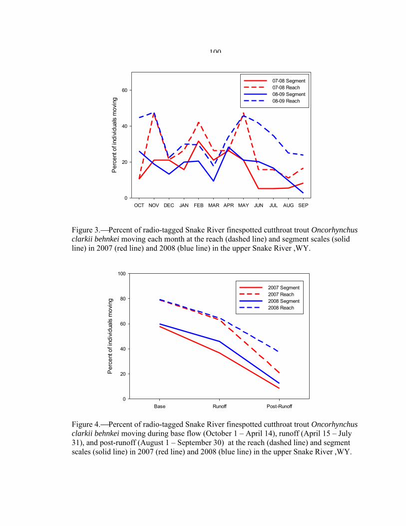
100
OCT NOV DEC JAN FEB MAR APR MAY JUN JUL AUG SEP
Per
cent
of i
ndiv
idua
ls m
ovin
g
0
20
40
60
07-08 Segment07-08 Reach08-09 Segment08-09 Reach
Figure 3.Percent of radio-tagged Snake River finespotted cutthroat trout Oncorhynchus
clarkii behnkei moving each month at the reach (dashed line) and segment scales (solid line) in 2007 (red line) and 2008 (blue line) in the upper Snake River ,WY.
Base Runoff Post-Runoff
Per
cent
of i
ndiv
idua
ls m
ovin
g
0
20
40
60
80
100
2007 Segment2007 Reach2008 Segment2008 Reach
Figure 4.Percent of radio-tagged Snake River finespotted cutthroat trout Oncorhynchus
clarkii behnkei moving during base flow (October 1 – April 14), runoff (April 15 – July 31), and post-runoff (August 1 – September 30) at the reach (dashed line) and segment scales (solid line) in 2007 (red line) and 2008 (blue line) in the upper Snake River ,WY.

101
Number of reaches moved
0 1-5 6-1011-15
16-2021-25
26-3031-35
36-4041-45
46-50> 50
Num
ber o
f ind
ividu
als
0
5
10
15
20
25
30
Figure 5.Annual sum of monthly movement distances (in reaches) by radio-tagged Snake River finespotted cutthroat trout Oncorhynchus clarkii behnkei (n = 94) in the Snake River, WY October 2007 – September 2009.
Number of segments moved
0 1 2 3 4 5 6 7 8 9 10 11 > 12
Num
ber o
f ind
ivid
uals
0
5
10
15
20
25
Figure 6.Annual sum of monthly movement distances (in segments) by radio-tagged Snake River finespotted cutthroat trout Oncorhynchus clarkii behnkei (n = 94) in the Snake River, WY October 2007 – September 2009.

102
Figure 7.Monthly reach occupancy of radio-tagged cutthroat trout Oncorhynchus
clarkii behnkei (n = 94) in the upper Snake River, WY October 2008 – September 2009. Monthly reach occupancy represents the total amount of time spent in each reach during each month by all individuals, collectively.

103
Figure 8.Principle coordinates analysis of monthly utilization distributions for all radio-tagged Snake River finespotted cutthroat trout Oncorhynchus clarkii behnkei
combined. The first component explained 99% of the variation among monthly utilization distributions and described differences in spatial patterns of time spent. The second component explained 1% of the variation and described differences between winter and summer utilization distributions.

104
Tables
Table 1.Physical habitat attributes (with methods and references) recorded in the upper Snake River during 2009 or derived using GIS based on 2009 LIDAR data.
Attribute Technique (reference)
Bank structure Total length of thalweg banks that are vertical (with vegetation) or undercut
Braid Index Total channel thalweg length of main channel and side channels divided by thalweg length of main channel (Knighton 1998)
Channel Form Number of side channels within each reach determined from 2009 NAIP imagery in GIS.
Confluences with Spring Creeks and Tributaries Number of confluences with spring creeks or tributaries within a reach (including downstream and upstream at reach breaks)
Constraint Ratio of bankfull width to flood-prone area width (Rosgen, 1994; Knighton 1998). Bankfull and flood-prone area polygons digitized in GIS based on identifiable geomorphic features. Where features were insufficient to delineate the edge of the floodplain, the polygon border was digitized at a maximum of 1 km from the edge of the bankfull channel.
Depth Data on maximum depth of each reach provided by Carl Legleitter.
Number of Fast Water Patches
Number of slow and fast water patches per unit length of reach (Hawkins et al. 1993). Patch must span > 50% of channel width to be counted.
Large Woody Debris (LWD)
To reflect the relationship between channel size and the size of woody debris that contributes to structure channels (Piegay 2003), LWD is defined as individual wood pieces or aggregates that are partially imbedded within a channel feature or that cause scour immediately downstream of the wood deposition site. Tally of single or aggregate pieces of LWD within each reach.
Macrophytes Thalweg length of channel where macrophytes extend across > 50% of the wetted width of the channel
Reach Thalweg Length Thalweg length from reach top to bottom obtained using GIS with reach locations overlayed on 2009 NAIP imagery
Sinuosity Straight-line reach length/ thalweg length calculated using GIS in main stem (Knighton 1998)
104

105 Table 2.Reach occupancy by radio-tagged Snake River finespotted cutthroat trout Oncorhynchus clarkii behnkei and physical characteristics of each stream reach in the upper Snake River from Jackson Lake Dam to Moose Junction, 2009.
Reach Segment Reach
occupancy
Thalweg length
(m) Braid index
Channel form Confluences
Number fast water patches Constraint Sinuosity
Large woody debris
Max depth (m) Macrophytes
Bank structure (m)
1 1 74 1843 1.00 0 3 0 2 1.21 3 4.0 0 562
2 1 48 742 2.35 2 0 6 2 1.15 22 2.0 0 75
3 1 34 408 1.52 0 0 0 1 1.00 66 2.0 0 232
4 1 54 506 2.87 2 0 1 1 1.01 100 3.0 0 157
5 1 152 767 1.00 0 0 0 1 1.18 8 6.9 0 396
6 1 1149 2047 1.49 3 1 0 2 7.01 204 6.0 2047 331
7 1 2037 2699 1.00 0 1 0 1 1.14 95 7.5 2699 525
8 2 145 414 1.00 0 1 1 2 1.01 26 1.5 0 256
9 2 197 609 1.35 4 0 0 1 0.98 65 1.7 0 452
10 2 699 2238 1.42 6 2 15 2 1.30 312 3.0 0 2404
11 2 919 1928 2.64 3 0 10 3 1.19 306 2.5 0 1246
12 2 794 1221 1.85 2 0 0 3 1.45 22 3.2 0 790
13 3 489 1054 1.00 0 2 0 1 1.00 6 2.4 0 284
14 3 302 729 2.56 1 0 5 3 1.22 41 1.6 0 609
15 3 111 323 1.00 0 0 0 3 1.22 7 2.3 0 346
16 3 345 978 3.32 4 0 16 3 1.17 148 2.4 0 511
17 3 224 818 1.00 0 0 1 5 1.62 19 2.9 0 329
18 3 98 435 1.84 1 0 1 5 1.15 22 2.2 0 306
19 3 43 209 1.00 0 0 0 8 1.05 3 1.7 0 0
20 3 79 419 1.62 1 0 4 4 1.02 14 1.7 0 348
105
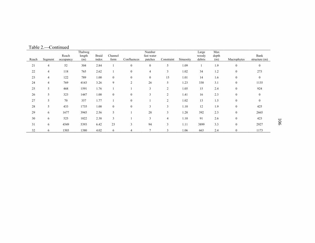
106 Table 2.Continued
Reach Segment Reach
occupancy
Thalweg length
(m) Braid index
Channel form Confluences
Number fast water patches Constraint Sinuosity
Large woody debris
Max depth (m) Macrophytes
Bank structure (m)
21 4 52 304 2.84 1 0 0 5 1.09 1 1.9 0 0
22 4 118 765 2.62 1 0 4 3 1.02 34 1.2 0 273
23 4 122 789 1.00 0 0 0 15 1.01 14 1.6 0 0 24 4 769 4143 3.26 9 2 26 5 1.23 330 3.1 0 1135
25 5 468 1591 1.76 1 1 3 2 1.05 15 2.4 0 924
26 5 323 1447 1.00 0 0 3 2 1.41 16 2.3 0 0
27 5 70 357 1.77 1 0 1 2 1.02 13 1.5 0 0
28 5 433 1735 1.00 0 0 3 3 1.10 12 1.9 0 425
29 6 1677 3945 2.56 5 1 28 3 1.28 392 2.3 0 2665
30 6 525 1022 2.38 3 1 3 4 1.10 91 2.6 0 423
31 6 4549 5393 6.42 23 3 94 3 1.11 3899 3.3 0 2927
32 6 1503 1380 4.02 6 4 7 3 1.06 663 2.4 0 1173
106
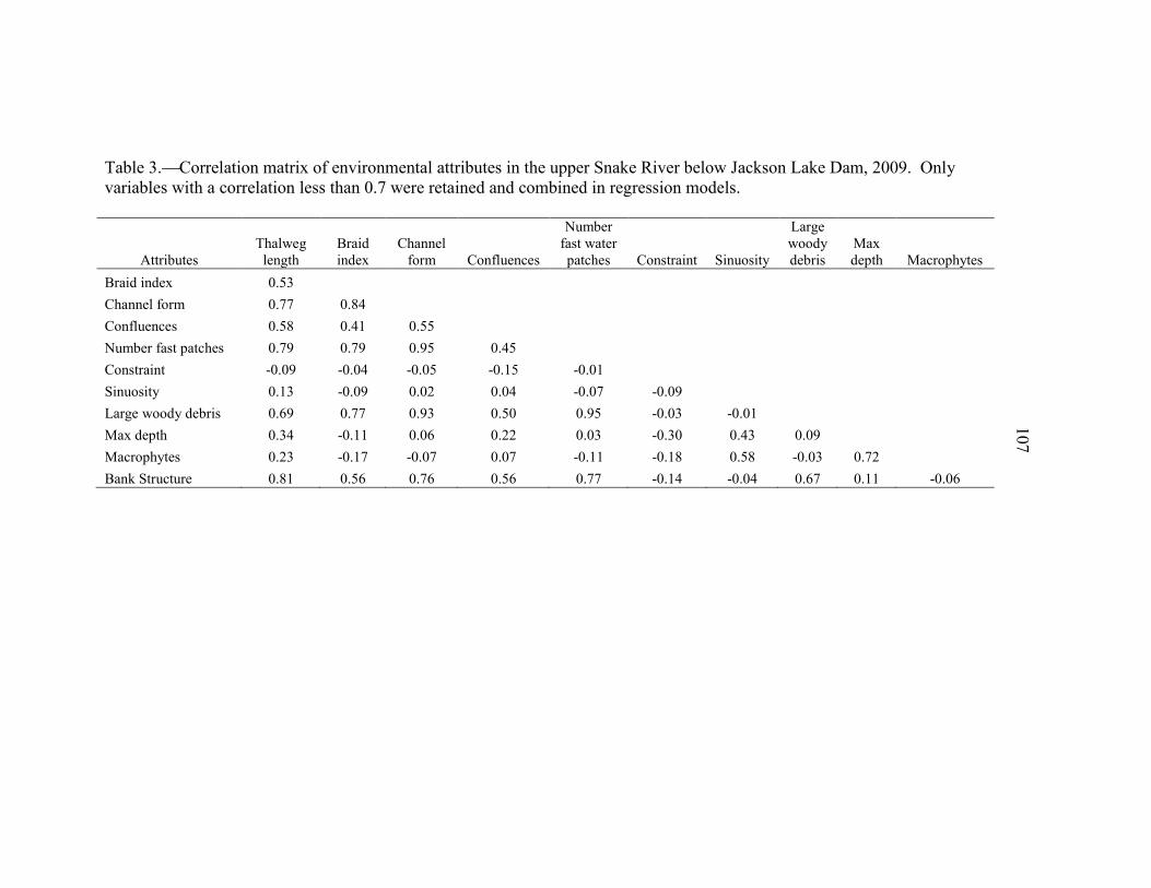
107
Table 3.Correlation matrix of environmental attributes in the upper Snake River below Jackson Lake Dam, 2009. Only variables with a correlation less than 0.7 were retained and combined in regression models.
Attributes Thalweg
length Braid index
Channel form Confluences
Number fast water patches Constraint Sinuosity
Large woody debris
Max depth Macrophytes
Braid index 0.53 Channel form 0.77 0.84
Confluences 0.58 0.41 0.55 Number fast patches 0.79 0.79 0.95 0.45
Constraint -0.09 -0.04 -0.05 -0.15 -0.01
Sinuosity 0.13 -0.09 0.02 0.04 -0.07 -0.09 Large woody debris 0.69 0.77 0.93 0.50 0.95 -0.03 -0.01
Max depth 0.34 -0.11 0.06 0.22 0.03 -0.30 0.43 0.09 Macrophytes 0.23 -0.17 -0.07 0.07 -0.11 -0.18 0.58 -0.03 0.72
Bank Structure 0.81 0.56 0.76 0.56 0.77 -0.14 -0.04 0.67 0.11 -0.06
107

108
Table 4.Candidate regression models to evaluate the relationship between habitat occupancy and reach-scale habitat attributes for Snake River finespotted cutthroat trout Oncorhynchus clarkii behnkei in the upper Snake River, WY 2009. The full dataset and Segments 2-6 datasets were evaluated with mixed effects models where segments were modeled as a random intercept. The Segment 1 dataset was evaluated with fixed effects models. Akaike’s information criterion (AIC) are presented for all models. The AIC (difference from top model) and r2 value (for the linear regression models with the Segment 1 dataset) are presented for models where all variables were significant. Segment 1 models were not nested, so AIC values were not presented. LWD = large woody debris, Depth = maximum depth, Banks = bank structure, and Mac = macrophytes.
Model AIC AIC DF Variance explained by random intercept
r2 of fixed effects
Full dataset Banks + Thalweg + LWD + Constraint + Sinuosity + Confluences + Depth +
Mac 221.8 - 18 0.69 - LWD + Constraint +Sinuosity + Confluences + Depth 215.9 - 21 0.46 - LWD + Constraint +Sinuosity + Confluences + Mac 223.3 - 21 0.37 - LWD + Depth 215.6 0 24 0.49 - Thalweg + Constraint +Sinuosity + Confluences + Depth 218.4 - 21 0.52 - Thalweg + Constraint +Sinuosity + Confluences + Mac 223.3 - 21 0.64 - Thalweg + Depth 218 2 24 0.54 - Banks + Constraint +Sinuosity + Confluences + Depth 233.6 - 21 0.20 - Banks + Constraint +Sinuosity + Confluences + Mac 236.4 - 21 0.25 - Banks + Depth 236.4 20 24 0.28 - Segments 2-6 dataset
Banks + Thalweg + LWD + Constraint + Sinuosity + Confluences + Depth 160.6 - 13 0.22 - LWD + Constraint +Sinuosity + Confluences + Depth 151.5 - 15 0.11 - LWD + Depth 155.8 0 18 0.26 - Thalweg + Constraint +Sinuosity + Confluences + Depth 156.4 - 15 0.47 - Thalweg + Depth 162.4 - 18 0.61 - Banks + Constraint +Sinuosity + Confluences + Depth 168.7 - 15 0.07 - Banks + Depth 176 20.2 18 0.31 -
108

109
Table 4. Continued
Model AIC AIC DF Variance explained by random intercept
Adjusted R2 of fixed effects
Segment 1 dataset Banks NA NA 5 NA -
Thalweg NA NA 5 NA 0.63 LWD NA NA 5 NA - Constraint NA NA 5 NA - Sinuosity NA NA 5 NA - Confluences NA NA 5 NA - Depth NA NA 5 NA 0.53 Macrophytes NA NA 5 NA 0.97
109
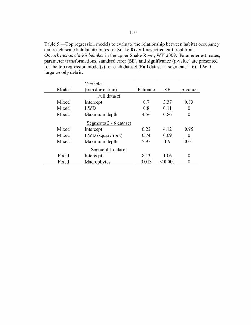
110 Table 5.Top regression models to evaluate the relationship between habitat occupancy and reach-scale habitat attributes for Snake River finespotted cutthroat trout Oncorhynchus clarkii behnkei in the upper Snake River, WY 2009. Parameter estimates, parameter transformations, standard error (SE), and significance (p-value) are presented for the top regression model(s) for each dataset (Full dataset = segments 1-6). LWD = large woody debris.
Model Variable (transformation) Estimate SE p-value
Full dataset
Mixed Intercept 0.7 3.37 0.83 Mixed LWD 0.8 0.11 0 Mixed Maximum depth 4.56 0.86 0
Segments 2 - 6 dataset
Mixed Intercept 0.22 4.12 0.95 Mixed LWD (square root) 0.74 0.09 0 Mixed Maximum depth 5.95 1.9 0.01
Segment 1 dataset
Fixed Intercept 8.13 1.06 0 Fixed Macrophytes 0.013 < 0.001 0

111
References Abbe, T. B. and D. R. Montgomery. 1996. Large woody debris jams, channel hydraulics
and habitat formation in large rivers. Regulated Rivers: Research and Management 12: 201-221.
Albanese, B., P. L. Angermeier, and S. Dorai-Raj. 2004. Ecological correlates of fish
movement in a network of Virginia streams. Canadian Journal of Fisheries and Aquatic Sciences 61: 857-869.
Bahr, M. A., and J. M. Shrimpton. 2004. Spatial and quantitative patterns of movement
in large bull trout (Salvelinus confluentus) from a watershed in north-western British Columbia, Canada, are due to habitat selection and not differences in life history. Ecology of Freshwater Fish 13: 294-304.
Baxter, C. V. and F. R. Hauer. 2000. Geomorphology, hyporheic exchange, and
selection of spawning habitat by bull trout (Salvelinus confluentus). Canadian Journal of Fisheries and Aquatic Sciences 57: 1470-1481.
Benda, L., N. L. Poff, D. Miller, T. Dunne, G. Reeves, G. Pess, and M. Pollock. 2004.
The network dynamics hypothesis: how channel networks structure riverine habitats. BioScience 54: 413-427.
Bozek, M. A. and F. J. Rahel. 1991. Assessing habitat requirements of young Colorado
River cutthroat trout by use of macrohabitat and microhabitat analyses. Transactions of the American Fisheries Society 120: 571-581.
Brenkman, S. J., J. J. Duda, C. E. Torgersen, E. Welty, G. R. Pess, R. Peters, and M. L.
McHenry. 2012. A riverscape perspective of Pacific salmonids and aquatic habitats prior to large-scale dam removal in the Elwha River, Washington, USA. Fisheries Management and Ecology, 19: 36–53.
Bult, T. P., R. I. Haedrich, and D. C. Schneider. 1998. New technique describing spatial
scaling and habitat selection in riverine habitats. Regulated Rivers: Research and Management 14: 107-118.
Burnham, K. P. and D. R. Anderson. 1998. Model selection and inference: an
information- theoretic approach. Spring-Verlag, New York. Carbonneau, P., M. A. Fonstad, W. A. Marcus, and S. J. Dugdale. 2011. Making
riverscapes real. Geomorphology 137: 74-86.

112 Carlson, A. J., and F. J. Rahel. 2010. Annual intrabasin movement and mortality of adult
Bonneville cutthroat trout among complementary riverine habitats. Transactions of the American Fisheries Society 139: 1360-1371.
Colyer, W. T., J. L. Kershner, and R. H. Hilderbrand. 2005. Movements of fluvial
Bonneville cutthroat trout in the Thomas Fork of the Bear River, Idaho–Wyoming. North American Journal of Fisheries Management 25: 954-963.
Dare, M. R. and W. A. Hubert. 2003. Use of similar habitat by cutthroat trout and brown
trout in a regulated river during winter. Northwest Science 77: 36-45. Ebersole, J. L., W. J. Liss, and C. A. Frissell. 2001. Relationship between stream
temperature, thermal refugia and rainbow trout Oncorhynchus mykiss abundance in arid-land streams in the northwestern United States. Ecology of Freshwater Fish 10: 1-10.
Ebersole, J. L., W. J. Liss, and C. A. Frissell. 2003. Thermal heterogeneity, stream
channel morphology, and salmonid abundance in Northeastern Oregon streams. Canadian Journal of Fisheries and Aquatic Sciences 60:1266-1280.
Fausch, K. D., C. E. Torgersen, C. V. Baxter, and H. W. Li. 2002. Landscapes to
riverscapes: bridging the gap between research and conservation of stream fishes. BioScience 52: 483-498.
Fretwell, S. D. 1972. Populations in a Seasonal Environment. Vol. 5. Princeton
University Press, Princeton, New Jersey. Frissell, C. A., W. J. Liss, C. E. Warren, and M. D. Hurley. 1986. A hierarchical
classification for stream habitat classification: viewing streams in a watershed context. Environmental Management 10: 199-214
Gomi, T., R. C. Sidle, and J. S Richardson. 2002. Understanding processes and
downstream linkages of headwater systems. Bioscience 52: 905-916 Gresswell, R. E., C. E. Torgersen, D. S. Bateman, T. J. Guy, S. R. Hendricks, and J. E. B.
Wofford. 2006. A spatially explicit approach for evaluating relationships among coastal cutthroat trout, habitat, and disturbance in small Oregon streams. American Fisheries Society Symposium 48: 457-471, Bethesda, MD.
Gresswell, R. E. and S. R. Hendricks. 2007. Population-scale movement of coastal
cutthroat trout in a naturally isolated stream network. Transactions of the American Fisheries Society 136: 238-253.

113 Harper, D. D. and A. M. Farag. 2004. Winter habitat use by cutthroat trout in the Snake
River near Jackson, Wyoming. Transactions of the American Fisheries Society 133: 15-25.
Heggenes, J., T. G. Northcote, and A. Peter. 1991. Spatial stability of cutthroat trout
(Oncorhynchus clarki) in a small, coastal stream. Canadian Journal of Fisheries and Aquatic Sciences 48: 757-762.
Henderson, R., J. L. Kershner, and C. A. Toline. 2000. Timing and location of spawning
by nonnative rainbow trout and native cutthroat trout in the South Fork Snake River, Idaho, with implications for hybridization. North American Journal of Fisheries Management 20: 584-96.
Homel, K., R. E. Gresswell, and J. L. Kershner. In prep-a. Life-history diversity of
Snake River finespotted cutthroat trout in the upper Snake River: implications for the conservation of native trout in a large river network
Homel, K., Homel, M. A., and R. E. Gresswell. In prep-b. Interpolating probabilistic
movement paths from sparse telemetry data in a linear system. Horan, D. L., J. L. Kershner, C. P. Hawkins, and T. A. Crowl. 2000. Effects of habitat
area and complexity on Colorado River cutthroat trout density in Uinta Mountain streams. Transactions of the American Fisheries Society 129: 1250-1263.
Hughes, N. F. 2000. Testing the ability of habitat selection theory to predict interannual
movement patterns of a drift-feeding salmonid. Ecology of Freshwater Fish 9: 4-8.
Isaak, D. J. and W. A. Hubert. 2001. A hypothesis about factors that influence
maximum summer stream temperatures across montane landscapes. Journal of the American Water Resources Association 37: 351-366.
Kershner, J. L., M. Coles-Ritchie, E. Cowley, R. C. Henderson, K. Kratz, C. Quimbly, D.
M. Turner, L. C. Ulmer, and M. R. Vinson. 2004. Guide to effective monitoring of aquatic and riparian resources. General Technical Report, RMRS-GTR-121, USDA, Forest Service, Rocky Mountain Research Station, Fort Collins, CO.
Kershner, J. L., C. M. Bischoff, and D. L. Horan. 1997. Population, habitat, and genetic
characteristics of Colorado River cutthroat trout in wilderness and nonwilderness stream sections in the Uinta Mountains of Utah and Wyoming. North American Journal of Fisheries Management 17: 1134-1143.
Knighton, D. 1998. Fluvial forms and processes. Oxford University Press, New York,
NY.

114 Kocik, J. F. and C. P. Ferreri. 1998. Juvenile production variation in salmonids:
population dynamics, habitat, and the role of spatial relationships. Canadian Journal of Fisheries and Aquatic Sciences 55(S1): 191–201.
Lowe, W. H., G. E. Likens, and M. E. Powers. 2006. Linking scales in stream ecology.
Bioscience 56: 591-597. Marcus, W. A., R. A. Marston, C. R. Colvard Jr., and R. D. Gray. 2002. Mapping the
spatial and temporal distributions of woody debris in streams of the Greater Yellowstone Ecosystem, USA. Geomorphology 44: 323-335.
Marston R. A., J. D. Mills, D. R. Wrazien, B. Bassett, D.K. Splinter. 2005. Effects of
Jackson Lake Dam on the Snake River and its floodplain, Grand Teton National Park, Wyoming, USA. Geomorphology 71: 79-98.
Montgomery, D.R., and J.M. Buffington, 1997, Channel-reach morphology in mountain
drainage basins, Geological Society of America Bulletin 109: 596-611. Montgomery D. R. 1999. Process domains and the river continuum. Journal of the
American Water Resources Association 35: 397-410. Nelson, N. C. 2007. Hydrology and geomorphology of the Snake River in Grand Teton
National Park, Wyoming. Masters thesis, Utah State University, Logan, UT, 133 pgs.
Northcote, R. G. 1997. Potamodromy in salmonidae living and moving in the fast lane.
North American Journal of Fisheries Management 17: 1029-1045. Petty, J. T., J. L. Hansbarger, B. M. Huntsman, and P. M. Mazik. 2012. Brook trout
movement in response to temperature, flow, and thermal refugia in a complex Appalachian riverscape. Transactions of the American Fisheries Society 141: 1060-1073.
Pinheiro, J., D. Bates, S. DebRoy, and D. Sarkar. 2012. nlme: Linear and nonlinear
mixed effects models, version 3.1-106, cran.r-project.org. Poff, N. L., and J. V. Ward. 1990. Physical habitat template of lotic systems: recovery in
the context of historical pattern of spatiotemporal heterogeneity. Environmental Management 14: 629–645.
Poole, G. C. 2002. Fluvial landscape ecology: addressing uniqueness within the river
discontinuum. Freshwater Biology 47: 641-660.

115 Pringle, C. M., R. J. Naiman, G. Bretschko, J. R. Karr, M. W. Oswood, J. R. Webster, R.
L. Welcomme, and M. J. Winterbourn. 1988. Patch dynamics in lotic systems: the stream as a mosaic. Journal of the North American Benthological Society 7: 503-524.
Rabeni, C. F., and S. P. Sowa. 1996. Integrating biological realism into habitat
restoration and conservation strategies for small streams. Canadian Journal of Fisheries and Aquatic Sciences 53 (suppl. 1): 252-259.
Roberts, D. W. 2012. labdsv: Ordination and multivariate analysis for ecology, version
1.5-0, cran.r-project.org. Rosgen, D. L. 1994. A classification of natural rivers. Catena 22: 169-199. Ross, M. J., and C. F. Kleiner. 1982. Shielded-needle technique for surgically
implanting radio-frequency transmitters in fish. Progressive Fish Culturist 44: 41-43.
Sanderson, T. B. and W. A. Hubert. 2009. Movements by adult cutthroat trout in a lotic
system: implications for watershed-scale management. Fisheries Management and Ecology 16: 329-336.
Schlosser, I. J. 1991. Stream fish ecology: a landscape perspective. BioScience 41: 704-
712. Schlosser, I. J. and P. L. Angermeier. 1995. Spatial variation in demographic processes in
lotic fishes: Conceptual models, empirical evidence, and implications for conservation. American Fisheries Society Symposium 17: 360–370.
Schmetterling, D. A. 2001. Seasonal movements of fluvial westslope cutthroat trout in
the Blackfoot River drainage, Montana. North American Journal of Fisheries Management 21:5 07-520.
Schoby, G. T., and E. R. Keeley. 2011. Home range size and foraging ecology of bull
trout and westslope cutthroat trout in the upper Salmon River basin, Idaho. Transactions of the American Fisheries Society 140: 636-645.
Schrank, A. J. and F. J. Rahel. 2004. Movement patterns in inland cutthroat trout:
management and conservation implications. Canadian Journal of Fisheries and Aquatic Sciences 61: 1528-1537.
Southwood, T. R. E. 1977. Habitat, the templet for ecological strategies. Journal of
Animal Ecology 46: 337-365.

116 Thorp, J. H., M. C. Thoms, and M. D. Delong. 2006. The riverine ecosystem synthesis:
biocomplexity in river networks across space and time. River Research and Applications 22: 123-147.
Thorp, J. H., J. E. Flotemersch, B. S. Williams, and L. A. Gabanski. 2013. Critical role
for hierarchical geospatial analyses in the design of fluvial research, assessment, and management. Environmental Monitoring and Assessment.
Torgersen, C. E., D. M. Price, H. W. Li, and B. A. McIntosh. 1999. Multiscale thermal
refugia and stream habitat associations of Chinook Salmon in Northeast Oregon. Ecological Applications 9: 301-319.
Torgersen, C. E., C. V. Baxter, H. W. Li, and B. A. McIntosh. 2006. Landscape
influences on longitudinal patterns of river fishes: spatially continuous analysis of fish-habitat relationships. American Fisheries Society Symposium 48: 473-492.
Townsend, C. R. 1996. Concepts in river ecology: pattern and process in the catchment
hierarchy. Archiv fu¨ r Hydrobiologie Supplement 113: 3–21. Van Kirk, R. W. and R. Martin. 2000. Interactions among aquatic vegetation, waterfowl,
flows, and the fishery below Island Park Dam. Intermountain Journal of Sciences 6: 249–262.
Vannote, R. L., G. W. Minshall, K. W. Cummins, J. R. Sedell, and C. E. Cushing. 1980.
The river continuum concept. Canadian Journal of Fisheries and Aquatic Sciences 37: 130-137.
Ward, J. V. and Stanford, J. A. 1983. 'The serial discontinuity concept of lotic
ecosystems' in Fontaine, T. D. and Barteli, S. M. (Editors), Dynamics of Lotic Ecosystems, Ann Arbor Science, Collingwood, MI. pp. 29-42.
Wiens, J. A. 1989. Spatial scaling in ecology. Functional Ecology 3: 385-397. Wiens, J. A. 2002. Riverine landscapes: taking landscape ecology into the water.
Freshwater Biology 47: 501-515. Young, M. K. 1996. Summer movements and habitat use by Colorado River cutthroat
trout (Oncorhynchus clarki pleuriticus) in small, montane streams. Canadian Journal of Fisheries and Aquatic Sciences 53: 1403-1408.
Zurstadt, C. and K. Stephan. 2004 Seasonal migration of westslope cutthroat trout in the
Middle Fork Salmon River drainage, Idaho. Northwest Science 78: 278-285.

117
CONCLUSION TO DISSERTATION
Native trout have experienced declines throughout their range as a result of
multiple anthropogenic factors (Gresswell 1988; Miller et al. 1989; Hudy et al. 2007).
Declines have been particularly pronounced for migratory trout that move through
degraded corridors or encounter downstream portions of the river network where all
upstream impacts are integrated (Thurow et al. 1997). In response to declines,
conservation and management of trout has focused on attributes associated with
population resiliency, including life-history diversity (Gresswell et al. 1994; Rieman and
Dunham 2000), and sufficient stream area to encompass the habitat needs throughout the
life-cycle (Hilderbrand and Kershner 2000a). For cutthroat trout in particular, most of
the existing research has occurred either in small streams at fine spatial scales
(Hilderbrand and Kershner 2000b; Brown and Mackay 1995; Gresswell 2009), or in
larger streams at coarser spatial scales (Colyer et al. 2005; Torgersen et al. 2012). Given
the need to understand life-history diversity and habitat occupancy in larger river
systems, it is not clear whether the patterns and variability in smaller streams can scale up
or serve as an analog for patterns in larger rivers.
In my dissertation, I studied the spatial ecology and life-history diversity of Snake
River finespotted cutthroat trout in the upper Snake River. The connectivity and high-
quality habitat in the river network, combined with the size of the river system and the
spatial variability, allowed me to assess specific relationships to habitat, life-history
diversity, and movement patterns. To do so, radio-telemetry was used to monitor the
movements of 248 cutthroat trout. In the course of analyzing these radio-telemetry data, I

118 encountered a set of common problems with this type of data, namely that data are sparse
and collected at an uneven sampling interval (Rogers and White 2007). Thus, I
collaborated on a statistical method that addressed these data problems and presented an
improved assessment of space use (that could feed into multiple types of analysis).
Collectively, the three papers in this dissertation provide an improved understanding of
life-history diversity, habitat occupancy, and movement patterns by native trout in a large
river network.
Principle Findings
In chapter 2, I explored the life-history diversity of Snake River finespotted
cutthroat trout in a large river network. Spawning and movement patterns reflected the
connectivity and habitat diversity of the Snake River study area and provided insight into
the range of life-history strategies that can be expressed in a spatiotemporally dynamic
system. Specifically, fluvial and fluvial-adfluvial spawners migrated to most of the
accessible spawning areas in the upper Snake River watershed, with the majority of
spawning between Buffalo Fork and Moose Junction. Post-spawning movement patterns
varied among individuals spawning in different streams or expressing different life-
history strategies.
In summary, cutthroat trout in this study inhabited and migrated through
substantial portions of the watershed and expressed a complex array of behavioral
strategies, although potential behaviors and accessible habitat were somewhat constrained
because of Jackson Lake Dam. The patterns observed here were substantially more

119 complex than what may be observed in a smaller system, suggesting that behavioral
diversity relates to the complexity of the physical template, and more so, that patterns
observed in smaller systems are not an analog for potential diversity in larger systems.
Ultimately, diversity in spawning, distribution, and movement patterns may be critical for
persistence in a variable environment (Den Boer 1968), particularly given the
uncertainties of climate change (Williams et al. 2009).
In chapter 3, I collaborated on a new interpolation method to address sparseness
and unevenness in the relocation data associated with radio-telemetry studies. This
adaptive kernel density interpolation method (AKDI) calculated a continuous probability
of time spent across the spatial domain of the data based on sparse sample data. Overall,
the AKDI method performed significantly better across sample sizes or sampling
frequencies in representing the “true” movement path than sample data, fixed kernel
density, or linear interpolation.
Irrespective of the interpolation method used, modeling results suggest that
interpolated utilization distributions were significantly better at describing the underlying
pattern of space-use than raw sample data. Currently, most telemetry studies in stream
systems quantify the number of relocations in spatial units (e.g., reaches) to describe
patterns of space-use, rather than analyze continuous, interpolated path data inclusive of
interior locations where individuals were never encountered. However, our modeling
results suggest that when movements are rapid, random, or frequent, use of raw point
data may produce significantly biased or potentially erroneous results. Thus, it appears

120 that interpolation methods may represent a significant improvement over existing
techniques in describing patterns of space-use in a linear system.
In chapter 4, I identified spatiotemporal movement patterns and spatial variation
in habitat occupancy by radio-tagged cutthroat trout in the upper Snake River.
Movements of adult nonspawning cutthroat trout predominantly occurred at the reach
scale during base flow and runoff conditions. However, these movements were typically
short (< 5 reaches or 1 segment) and did not result in substantial changes to the monthly
utilization distribution of time spent by all individuals in each reach. Reach-scale habitat
occupancy varied within and among segments. Where channels were complex with
increased gradient, velocity, and sediment or wood delivery, reach occupancy was
associated with large woody debris and the maximum depth of a reach. However, where
the channel was simple and quasi-lentic, reach occupancy was associated with the length
of the reach dominated by submerged macrophytes. Consequently, it appeared that the
availability of habitat varied spatially and the function of habitat varied in response to the
constraining effects of segment-scale attributes.
Given the spatial and hierarchical variation in habitat availability and function
observed in this study, it was apparent that throughout the physical template, reaches or
segments were not experimental replicates; rather, contextual variation in the physical
template resulted in contextual habitat relationships. Consequently, the following
recommendations could improve assessment of habitat occupation and movement
patterns in river networks. First, a focus on functional habitat relationships (Schlosser
1991; Northcote 1997) may be more transferable across systems than one based on

121 attributes. Second, spatial processes should be explicitly incorporated in analysis as they
set the context for observed behaviors (Fausch et al. 2002, Poole 2002; Brenkman et al
2012). Third, in evaluating spatial data, utilization distributions (e.g., as created by
AKDI) may provide a useful method to incorporate uncertainty into observed habitat
occupancy or movement patterns. Finally, hierarchical and spatial variation in
disturbance regimes (Frissell et al. 1986; Gomi et al. 2002) suggests that small streams
are not comparable to large streams just as fine spatial scales are not comparable to
coarse spatial scales.
Summary
In synthesizing these chapters, several common themes emerged. First, there was
consistent evidence that the upper Snake River is a very complex system that may be
representative of other intermediate sized river networks that are in a relatively pristine
condition. Against this backdrop of complexity, spatiotemporal variation in the physical
template created a range of habitat attributes and functions. In response to the spatial
availability of habitat, cutthroat trout expressed complex life-history strategies and
variation in habitat occupancy and movement patterns. However, this diversity
illustrated the importance of conceiving life-history diversity more broadly than the
categorical descriptions (based on spawning and rearing habitat) that are commonly used.
Moreover, movement patterns expressed by spawners and nonspawners differed
considerably during both spawning and nonspawning time periods, suggesting that it is

122 important to consider these stages independently when evaluating habitat occupation and
movement.
Collectively, variation in spawning, habitat occupancy, and movement patterns
allows a complex response to a dynamic template and is often linked to increased
population persistence through spreading extirpation risk from natural causes (Den Boer
1968). Certainly, the spatial range of habitats occupied in this study would suggest that
local disturbances (e.g., debris torrent in a tributary) would not have a population-level
consequence. However, other threats to persistence, such as introduced species or
climate change, may operate at a larger spatial scale. Consequently, there is a need to
balance management for diversity and spatial variation to minimize extirpation risk from
spatially discrete, local disturbances, with consideration of specific actions that could
minimize risk from regional disturbances (e.g., climate change or invasive species). The
challenge is that the same actions that may prevent hybridization (e.g., barriers), may
reduce the capacity to respond to a changing climate where complex habitats (particularly
thermal refugia) and large habitat patches (Cowley 2008) may be required. As such,
management for maintaining diversity in the physical template (Poff et al. 1997; Ebersole
et al. 1997) and preservation of the connectivity that permits life-history diversity (Den
Boer 1968; Warren and Liss 1980) may be effective at achieving population resiliency
(Hilborn et al. 2003). However, targeted removal of invasive species (Bennett and
Kershner 2009) or targeted isolation of portions of river networks may be required as
well (Muhlfeld et al. 2012).

123
References
Bennett, S. and J.L. Kershner. 2009. Levels of introgression in Westslope cutthroat populations eight years after changes to rainbow trout stocking programs in southeastern British Columbia. North American Journal of Fisheries Management 29:1271-1282.
Brenkman, S. J., J. J. Duda, C. E. Torgersen, E. Welty, G. R. Pess, R. Peters, and M. L.
McHenry. 2012. A riverscape perspective of Pacific salmonids and aquatic habitats prior to large-scale dam removal in the Elwha River, Washington, USA. Fisheries Management and Ecology, 19: 36–53.
Brown, R.S. and W.C. Mackay. 1995. Fall and winter movements of and habitat use by
cutthroat trout in the Ram River, Alberta. Transactions of the American Fisheries Society 124:873-885.
Colyer, W. T., J. L. Kershner, and R. H. Hilderbrand. 2005. Movements of fluvial
Bonneville cutthroat trout in the Thomas Fork of the Bear River, Idaho–Wyoming. North American Journal of Fisheries Management 25:954-963.
Cowley, D. E. 2008. Estimating required habitat size for fish conservation in streams.
Aquatic Conservation: Marine and Freshwater Ecosystems 18(4): 418-431. Den Boer, P. J. 1968. Spreading of risk and stabilization of animal numbers. Acta
Biotheoretica 18:165-194 Ebersole, J. L., W. J. Liss, and C. A. Frissell. 1997. Restoration of stream habitats in the
Western United States: restoration as reexpression of habitat capacity. Environmental Management 21: 1-14.
Fausch K. D., C. E. Torgersen, C. V. Baxter, and H. W. Li. 2002. Landscapes to
riverscapes: bridging the gap between research and conservation of stream fishes. Bioscience 52(6):483-98.
Frissell, C. A., W. J. Liss, C. E. Warren, and M. D. Hurley. 1986. A hierarchical
classification for stream habitat classification: viewing streams in a watershed context. Environmental Management 10: 199-214.
Gomi, T., R. C. Sidle, and J. S Richardson. 2002. Understanding processes and
downstream linkages of headwater systems. Bioscience 52: 905-916 Gresswell, R. E., editor. 1988. Status and management of interior stocks of cutthroat
trout. American Fisheries Society Symposium 4: 45-52.

124 Gresswell R. E., W. J. Liss, and D. L. Larson. 1994. Life-History Organization of
Yellowstone Cutthroat Trout (Oncorhynchus clarki bouvieri) in Yellowstone Lake. Canadian Journal of Fisheries and Aquatic Sciences 51 (Suppl. 1):298-309.
Gresswell, R. E. 1999. Fire and aquatic ecosystems in forested biomes of North
America. Transactions of the American Fisheries Society 128: 193-221. Hilderbrand, R. H., and Kershner, J. L., 2000a, Conserving inland cutthroat trout in small
streams: how much stream is enough?: North American Journal of Fisheries Management 20:513-520.
Hilderbrand, R. H., and Kershner, J. L., 2000b, Movement patterns of stream-resident
cutthroat trout in Beaver Creek, Idaho-Utah: Transactions of the American Fisheries Society 129:1160-1170.
Hilborn, R., T. P. Quinn, D. E. Schindler, and D. E. Rogers. 2003. Biocomplexity and
fisheries sustainability. Proceedings of the National Academy of Science 100: 6564-6568.
Hudy, M., B. Roper, and N. Gillespie. 2007. Large scale assessments: lessons learned for
native trout management. Proceedings of Wild Trout Symposium IX, West Yellowstone, MT October 2007.
Miller, R. R., J. D. Williams, and J. E. Williams. 1989. Extinctions of North American
fishes during the last century. Fisheries 12:22-38. Muhlfeld, C. C., V. D’Angelo, S. T. Kalinowski, E. L. Landguth, C. C. Downs, J. Tohtz,
and J. L. Kershner. 2012. A fine-scale assessment of using barriers to conserve native stream salmonids: a case study in Akokala Creek, Glacier National Park, USA. The Open Fish Science Journal 5:9-20.
Northcote, T. G. 1997. Potamodromy in Salmonidae- living and moving in the fast lane.
North American Journal of Fisheries Management 17: 1029-1045. Poff, N. L., J. D. Allan, M. B. Bain, J. R. Karr, K. L. Prestegaard, B. D. Richter, R. E.
Sparks, and J. C. Stromberg. 1997. The natural flow regime: a paradigm for river conservation and restoration. BioScience 47: 769-784.
Poole, G.C. 2002. Fluvial Landscape Ecology: Addressing Uniqueness within the River
Discontinuum. . Freshwater Biology. 47(4): 641-660.

125 Rieman, B. E. and J. B. Dunham. 2000. Metapopulations and salmonids: a synthesis of
life history patterns and empirical observations. Ecology of Freshwater Fish 9: 51–64.
Rogers, K. B., and G. C. White. 2007. Analysis of movement and habitat use from
telemetry data in C. S. Guy and M. L. Brown, editors. Analysis and interpretation of freshwater fisheries data. American Fisheries Society, Bethesda, Maryland, USA.
Saiget, D. A., M. R. Sloat, and G. H. Reeves. 2007. Spawning and movement behavior
of migratory coastal cutthroat trout on the Western Copper River Delta, Alaska. North American Journal of Fisheries Management 27:1029-1040.
Schlosser, I. J. 1991. Stream fish ecology: a landscape perspective. BioScience 41: 704-
712. Thurow, R. F., D. C. Lee, and B. E. Rieman. 1997. Distribution and status of seven
native salmonids in the interior Columbia River basin and portions of the Klamath River and Great Basins, North American Journal of Fisheries Management 17(4) 1094-1110.
Torgersen, C.E., C.V. Baxter, J.L. Ebersole, and R.E. Gresswell. 2012. Incorporating
spatial context into the analysis of salmonid-habitat relationships. Pages 216-224 in M. Church, P.M. Biron, and A. Roy, editors. Gravel-bed rivers: Processes, tools, environments. John Wiley & Sons Limited, Chichester, UK.
Warren C. E. and W. J. Liss. 1980. Adaptation to aquatic environments. Pages 15-40 in
R. T. Lackey, and L. Nielsen, editors. Fisheries Management. Oxford, UK: Blackwell Scientific Publications.
Williams, J.E., A.L. Haak, H.M. Neville, and W.T. Coyler. 2009. Potential
consequences of climate change to persistence of cutthroat trout populations. North American Journal of Fisheries Management 29: 533-548.

126
REFERENCES CITED

127 Abbe, T.B. and D.R. Montgomery. 1996. Large woody debris jams, channel hydraulics
and habitat formation in large rivers. Regulated Rivers: Research and Management 12:201-221.
Addicott, J. F., J. M. Aho, M. F. Antolin, D. K. Padilla, J. S. Richardson, and D. A.
Soluk. 1987. Ecological neighborhoods: scaling environmental patterns. Oikos 49:340-346.
Albanese, B., P. L. Angermeier, and S. Dorai-Raj. 2004. Ecological correlates of fish
movement in a network of Virginia streams. Canadian Journal of Fisheries and Aquatic Sciences 61: 857-869.
Bahr, M. A., and J. M. Shrimpton. 2004. Spatial and quantitative patterns of movement
in large bull trout (Salvelinus confluentus) from a watershed in north-western British Columbia, Canada, are due to habitat selection and not differences in life history. Ecology of Freshwater Fish 13: 294-304.
Baxter, C. V. and F. R. Hauer. 2000. Geomorphology, hyporheic exchange, and
selection of spawning habitat by bull trout (Salvelinus confluentus). Canadian Journal of Fisheries and Aquatic Sciences 57: 1470-1481.
Behnke, R. J. 1992. Native trout of western North America. American Fisheries Society
Monograph 6. Benda, L., N.L. Poff, D. Miller, T. Dunne, G. Reeves, G. Pess, and M. Pollock. 2004.
The network dynamics hypothesis: how channel networks structure riverine habitats. BioScience 54:413-427.
Benhamou, S. 2011. Dynamic approach to space and habitat use based on biased
random bridges. Plos One 6(1): e14592. Bennett, S. and J.L. Kershner. 2009. Levels of introgression in Westslope cutthroat
populations eight years after changes to rainbow trout stocking programs in southeastern British Columbia. North American Journal of Fisheries Management 29:1271-1282.
Bozek, M. A. and F. J. Rahel. 1991. Assessing habitat requirements of young Colorado
River cutthroat trout by use of macrohabitat and microhabitat analyses. Transactions of the American Fisheries Society 120:571-581.
Brenkman, S. J., G. R. Pess, C. E. Toregersen, K. K. Kloehnd, J. J. Dudae, and S. C.
Corbett. 2008. Predicting recolonization patterns and interactions between potamodromous and anadromous salmonids in response to dam removal in the Elwha River, Washington State, USA. Northwest Science 82(sp1):91-106.

128 Brenkman, S. J., J. J. Duda, C. E. Torgersen, E. Welty, G. R. Pess, R. Peters, and M. L.
McHenry. 2012. A riverscape perspective of Pacific salmonids and aquatic habitats prior to large-scale dam removal in the Elwha River, Washington, USA. Fisheries Management and Ecology, 19: 36–53.
Brown, R.S. and W.C. Mackay. 1995. Fall and winter movements of and habitat use by
cutthroat trout in the Ram River, Alberta. Transactions of the American Fisheries Society 124:873-885.
Bullard F. 1999. Estimating the home range of an animal: a Brownian bridge approach.
Thesis. University of North Carolina, Chapel Hill, North Carolina, USA. Bult, T. P., R. I. Haedrich, and D. C. Schneider. 1998. New technique describing spatial
scaling and habitat selection in riverine habitats. Regulated Rivers: Research and Management 14: 107-118.
Burnham, K. P. and D. R. Anderson. 1998. Model selection and inference: an
information- theoretic approach. Spring-Verlag, New York. Carbonneau, P., M. A. Fonstad, W. A. Marcus, and S. J. Dugdale. 2011. Making
riverscapes real. Geomorphology 137: 74-86. Carlson, A. J. and F. J. Rahel. 2010. Annual intrabasin movement and mortality of adult
Bonneville cutthroat trout among complementary riverine habitats. Transactions of the American Fisheries Society 139: 1360-1371.
Cole, L. C. 1954 The population consequences of life-history phenomena. The
Quarterly Review of Biology 29: 103-137. Colyer, W. T., J. L. Kershner, and R. H. Hilderbrand. 2005. Movements of fluvial
Bonneville cutthroat trout in the Thomas Fork of the Bear River, Idaho–Wyoming. North American Journal of Fisheries Management 25:954-963.
Cowley, D. E. 2008. Estimating required habitat size for fish conservation in streams.
Aquatic Conservation: Marine and Freshwater Ecosystems 18(4): 418-431. Cuddington, K. and P. Yodzis. 2002. Predator–prey dynamics and movement in fractal
environments. American Naturalist 160: 119–134. Dare, M. R. and W. A. Hubert. 2003. Use of similar habitat by cutthroat trout and brown
trout in a regulated river during winter. Northwest Science 77:36-45.

129 Den Boer, P. J. 1968. Spreading of risk and stabilization of animal numbers. Acta
Biotheoretica 18:165-194 DeRito, J. N., A. V. Zale, and B. B. Shepard. 2010. Temporal reproductive separation of
fluvial Yellowstone cutthroat trout from rainbow trout and hybrids in the Yellowstone River. North American Journal of Fisheries Management 30:866-886.
de Solla, S. R., R. Bonduriansky, and R. J. Brooks. 1999. Eliminating autocorrelation
reduces biological relevance of home range estimates. Journal of Animal Ecology 68: 221-234.
Downs, J. A. 2010. Time-geographic density estimation for moving point objects.
Lecture Notes in Computer Science 6292: 16-26. Ebersole, J. L., W. J. Liss, and C. A. Frissell. 1997. Restoration of stream habitats in the
Western United States: restoration as reexpression of habitat capacity. Environmental Management 21: 1-14.
Ebersole, J. L., W. J. Liss, and C. A. Frissell. 2001. Relationship between stream
temperature, thermal refugia and rainbow trout Oncorhynchus mykiss abundance in arid-land streams in the northwestern United States. Ecology of Freshwater Fish 10:1-10.
Ebersole, J. L., W. J. Liss, and C. A. Frissell. 2003. Thermal heterogeneity, stream
channel morphology, and salmonid abundance in Northeastern Oregon streams. Canadian Journal of Fisheries and Aquatic Sciences 60:1266-1280.
Fausch K. D., C. E. Torgersen, C. V. Baxter, and H. W. Li. 2002. Landscapes to
riverscapes: bridging the gap between research and conservation of stream fishes. Bioscience 52(6):483-98.
Fieberg, J. 2007. Kernel density estimators of home range use: smoothing and the
autocorrelation red herring. Ecology 88: 1059-1066. Fieberg, J., J. Matthiopoulos, M. Hebblewhite, M. S. Boyce, and J. L. Frair. 2010.
Correlation and studies of habitat selection: problem, red herring, or opportunity? Philosophical Transactions of the Royal Society B 365: 2233-2244.
Fretwell, S. D. 1972. Populations in a seasonal environment. Princeton University Press,
Princeton, NJ.

130 Frissell, C. A., W. J. Liss, C. E. Warren, and M. D. Hurley. 1986. A hierarchical
classification for stream habitat classification: viewing streams in a watershed context. Environmental Management 10: 199-214.
Garton, E. O., M. J. Wisdom, F. A. Leban, and B. K. Johnson. 2001. Experimental
design for radiotelemetry studies. Pages 15-42 in J. J. Millspaugh and J. M. Marsluff, editors. Radio tracking and animal populations. Academic Press, San Diego, California, USA.
Gomi, T., R. C. Sidle, and J. S Richardson. 2002. Understanding processes and
downstream linkages of headwater systems. Bioscience 52: 905-916 Grant, E. H. C., W. H. Lowe, and W. F. Fagan. 2007. Living in the branches: population
dynamics and ecological processes in dendritic networks. Ecology Letters 10: 165-175.
Greene, C. M., J. E. Hall, K. R. Guilbault, and T. P. Quinn. 2010. Improved viability of
populations with diverse life-history portfolios. Biology Letters 6: 382-386. Gregory, J. and S. Yates. 2009. Trout movement in the Gros Ventre River and access to
the Snake River. Final Draft Report produced by Gregory Aquatics for Trout Unlimited. September 2009.
Gresswell, R. E., editor. 1988. Status and management of interior stocks of cutthroat
trout. American Fisheries Society Symposium 4: 45-52. Gresswell, R. E. and J. D. Varley. 1988. Effects of a century of human influence on the
cutthroat trout of Yellowstone Lake. American Fisheries Society Symposium 4: 45-52.
Gresswell R. E., W. J. Liss, and D. L. Larson. 1994. Life-History Organization of
Yellowstone Cutthroat Trout (Oncorhynchus clarki bouvieri) in Yellowstone Lake. Canadian Journal of Fisheries and Aquatic Sciences 51 (Suppl. 1):298-309.
Gresswell, R. E., W. J. Liss, G. L. Larson, and P. J. Bartlein. 1997. Influence of basin-
scale physical variables on life history characteristics of cutthroat trout in Yellowstone Lake. North American Journal of Fisheries Management 17:1046-1064.
Gresswell, R. E. 1999. Fire and aquatic ecosystems in forested biomes of North
America. Transactions of the American Fisheries Society 128: 193-221. Gresswell, R. E., C. E. Torgersen, D. S. Bateman, T. J. Guy, S. R. Hendricks, and J. E. B.
Wofford. 2006. A spatially explicit approach for evaluating relationships among

131
coastal cutthroat trout, habitat, and disturbance in small Oregon streams. American Fisheries Society Symposium 48:457-471, Bethesda, MD.
Gresswell, R. E. and S. R. Hendricks. 2007. Population-scale movement of coastal
cutthroat trout in a naturally isolated stream network. Transactions of the American Fisheries Society 136:238-253.
Gresswell, R.E. 2009. Yellowstone Cutthroat Trout (Oncorhynchus clarkii bouvieri): A
Technical Conservation Assessment [Online]. USDA Forest Service, Rocky Mountain Region. Available: http://www.fs.fed.us/r2/projects/scp/assessments/yellowstonecutthroattrout.pdf [27 June 2009].
Gresswell, R. E. 2011. Biology, Status, and Management of the Yellowstone Cutthroat
Trout. North American Journal of Fisheries Management, 31:5, 782-812. Gross, M. R. 1991. Salmon breeding behavior and life-history evolution in changing
environments. Ecology 72(4): 1180-1186. Harper, D. D. and A. M. Farag. 2004. Winter habitat use by cutthroat trout in the Snake
River near Jackson, Wyoming. Transactions of the American Fisheries Society 133, 15-25.
Hayden, P. S. 1967. The reproductive behavior of the Snake River cutthroat trout in
three tributary streams in Wyoming. Wyoming Game and Fish Commission, Cooperative Research Project 4. 105 pp.
Heggenes, J., T. G. Northcote, and A. Peter. 1991. Spatial stability of cutthroat trout
(Oncorhynchus clarki) in a small, coastal stream. Canadian Journal of Fisheries and Aquatic Sciences 48:757-762.
Henderson, R., J. L. Kershner, and C. A. Toline. 2000. Timing and location of spawning
by nonnative rainbow trout and native cutthroat trout in the South Fork Snake River, Idaho, with implications for hybridization. North American Journal of Fisheries Management 20:584-96.
Hilderbrand, R. H., and Kershner, J. L., 2000a, Conserving inland cutthroat trout in small
streams: how much stream is enough?: North American Journal of Fisheries Management 20:513-520.
Hilderbrand, R. H., and Kershner, J. L., 2000b, Movement patterns of stream-resident
cutthroat trout in Beaver Creek, Idaho-Utah: Transactions of the American Fisheries Society 129:1160-1170.

132 Hilborn, R., T. P. Quinn, D. E. Schindler, and D. E. Rogers. 2003. Biocomplexity and
fisheries sustainability. Proceedings of the National Academy of Science 100: 6564-6568.
Hitt, N.P., P.L. Angermeier. 2006. Effects of adjacent streams on local fish assemblage
structure in Western Virginia: implications for biomonitoring. American Fisheries Society Symposium 48: 75-86.
Hodder, K. H., J. E. G. Masters, W. R. C. Beaumont, R. E. Gozlan, A. C. Pinder, C. M.
Knight, and R. E. Kenward. 2007. Techniques for evaluating the spatial behaviour of river fish. Hydrobiologia 582: 257-269.
Horan, D. L., J. L. Kershner, C. P. Hawkins, and T. A. Crowl. 2000. Effects of habitat
area and complexity on Colorado River cutthroat trout density in Uinta Mountain streams. Transactions of the American Fisheries Society 129: 1250-1263.
Horne, J. S., E. O. Garton, S. M. Krone, and J. S. Lewis. 2007. Analyzing animal
movements using Brownian bridges. Ecology 88(9): 2354-2363. Hubert, W. A., J. C. Burckhardt, M. P. Joyce, R. Gipson, D. Zafft, D. Hawk, and D.
Money. 2001. Whirling disease among Snake River cutthroat trout in spring streams in Wyoming pages 80-82 in 2001 Whirling Disease Symposium, Montana State University.
Hudy, M., B. Roper, and N. Gillespie. 2007. Large scale assessments: lessons learned for
native trout management. Proceedings of Wild Trout Symposium IX, West Yellowstone, MT October 2007.
Hughes, N. F. 2000. Testing the ability of habitat selection theory to predict interannual
movement patterns of a drift-feeding salmonid. Ecology of Freshwater Fish 9: 4-8.
Isaak, D. J. and W. A. Hubert. 2001. A hypothesis about factors that influence
maximum summer stream temperatures across montane landscapes. Journal of the American Water Resources Association 37:351-366.
Johnson, D. H. 1980. The comparison of usage and availability measurements for
evaluating resource preference. Ecology 61: 65-71. Johnson, A. R., J. A. Wiens, B. T. Milne, and T. O. Crist. 1992. Animal movements and
population dynamics in heterogeneous landscapes. Landscape Ecology 7(1): 63-75.

133 Johnson, D. S., J. M. London, M. Lea, and J. W. Durban. 2008a. Continuous-time
correlated random walk model for animal telemetry data. Ecology 89(5): 1208-1215.
Johnson D. S., D. L. Thomas, J. M. Ver Hoef, and A. Christ. 2008b. A general
framework for the analysis of animal resource selection from telemetry data. Biometrics 64: 968-976.
Jonsen, I. D., R. A. Myers, and J. M. Flemming. 2003. Meta-analysis of animal
movement using state-space models. Ecology 84(11): 3055-3063. Joyce, M. P. and W. A. Hubert. 2004. Spawning ecology of finespotted Snake River
cutthroat trout in spring streams of the Salt River valley, Wyoming. Western North American Naturalist 64:78-85.
Kaitala, A., V. Kaitala, and P. Lundberg. 1993. A theory of partial migration. The
American Naturalist 142: 59-81. Keating, K. A., and S. Cherry. 2009. Modeling utilization distributions in space and
time. Ecology 90(7): 1971-1980. Kershner, J. L., M. Coles-Ritchie, E. Cowley, R. C. Henderson, K. Kratz, C. Quimbly, D.
M. Turner, L. C. Ulmer, and M. R. Vinson. 2004. Guide to effective monitoring of aquatic and riparian resources. General Technical Report, RMRS-GTR-121, USDA, Forest Service, Rocky Mountain Research Station, Fort Collins, CO.
Kershner, J. L., C. M. Bischoff, and D. L. Horan. 1997. Population, habitat, and genetic
characteristics of Colorado River cutthroat trout in wilderness and nonwilderness stream sections in the Uinta Mountains of Utah and Wyoming. North American Journal of Fisheries Management 17:1134-1143.
Kiefling, J.W. 1978. Studies on the ecology of the Snake River cutthroat trout. Fisheries
Technical Bulletin No.3, Wyoming Game and Fish Department, Cheyenne, Wyoming.
Knighton, D. 1998. Fluvial forms and processes. Oxford University Press, New York,
NY. Kocik, J. F. and C. P. Ferreri. 1998. Juvenile production variation in salmonids:
population dynamics, habitat, and the role of spatial relationships. Canadian Journal of Fisheries and Aquatic Sciences 55(S1): 191–201.

134 Kovach, R. , L. Eby, and M. P. Corsi. 2011. Hybridization between Yellowstone
cutthroat trout and rainbow trout in the upper Snake River basin, Wyoming. North American Journal of Fisheries Management 31: 1077-1087.
Kruse, C. G., W. A. Hubert, and F. J. Rahel. 1997. Geomorphic influences on the
distribution of Yellowstone Cutthroat trout in the Absaroka Mountains, Wyoming. Transactions of the American Fisheries Society 126: 418-427.
Kruse, C. G., W. A. Hubert, and F. J. Rahel. 2000. Status of Yellowstone cutthroat trout
in Wyoming waters. North American Journal of Fisheries Management 20: 693-705.
Levin, S. 1992. The problem of pattern and scale in ecology: The Robert H. MacArthur
Award Lecture. Ecology 73: 1943-1967. Loudenslager, E. J., and R. M. Kitchin. 1979. Genetic similarity of two forms of
cutthroat trout, Salmo clarki, in Wyoming. Copeia 1979: 673-678. Lowe, W. H., G. E. Likens, and M. E. Powers. 2006. Linking scales in stream ecology.
Bioscience 56: 591-597. Lucas, M. C. and E. Baras. 2000. Methods for studying the spatial behavior or
freshwater fishes in the natural environment. Fish and Fisheries 1: 283-316. MacArthur, R.H. and E.O. Wilson. 1967. The Theory of Island Biogeography.
Princeton, New Jersey: Princeton Univ. Press. 203 pp. Manly, B. F., L. McDonald, D. Thomas, T. McDonald, and W. Erickson. 2002.
Resource selection by animals: statistical design and analysis for field studies. Kluwer Academic Publishers, Boston, Massachusetts, USA.
Marcus, W. A., R. A. Marston, C. R. Colvard Jr., and R. D. Gray. 2002. Mapping the
spatial and temporal distributions of woody debris in streams of the Greater Yellowstone Ecosystem, USA. Geomorphology 44: 323-335.
Marston R. A., J. D. Mills, D. R. Wrazien, B. Bassett, D. K. Splinter. 2005. Effects of
Jackson Lake Dam on the Snake River and its floodplain, Grand Teton National Park, Wyoming, USA. Geomorphology 71: 79-98.
McGrath, C. C. and W. M. Lewis Jr. 2007. Competition and predation as mechanisms
for displacement of greenback cutthroat trout by brook trout. Transactions of the American Fisheries Society 136: 1381-1392.

135 Meka, J. M., E. E. Knudsen, D. C. Douglas, and R. B. Benter. 2003. Variable migratory
patterns of different adult rainbow trout life-history types in a Southwest Alaska watershed. Transactions of the American Fisheries Society 132: 717-732.
Miller, R. R., J. D. Williams, and J. E. Williams. 1989. Extinctions of North American
fishes during the last century. Fisheries 12: 22-38. Millspaugh, J. J., R. M. Nielson, L. McDonald, J. M. Marzluff, R. A. Gitzen, C. D.
Rittenhouse, M. W. Hubbard, and S. L. Sheriff. 2006. Analysis of resource selection using utilization distributions. The Journal of Wildlife Management 70: 384-395.
Montgomery, D.R., and J.M. Buffington, 1997, Channel-reach morphology in mountain
drainage basins, Geological Society of America Bulletin, 109: 596-611. Montgomery D. R. 1999. Process domains and the river continuum. Journal of the
American Water Resources Association 35: 397-410. Muhlfeld, C. C., T. E. McMahon, M. C. Boyer, and R. E. Gresswell. 2009. Local
habitat, watershed, and biotic factors influencing the spread of hybridization between native westslope cutthroat trout and introduced rainbow trout. Transactions of the American Fisheries Society 138: 1036-1051.
Muhlfeld, C. C., V. D’Angelo, S. T. Kalinowski, E. L. Landguth, C. C. Downs, J. Tohtz,
and J. L. Kershner. 2012. A fine-scale assessment of using barriers to conserve native stream salmonids: a case study in Akokala Creek, Glacier National Park, USA. The Open Fish Science Journal 5:9-20.
Muneepeerakul, R., E. Bertuzzo, H. J. Lynch, W. F. Fagan, A.Rinaldo, and I. Rodriguez-
Iturbe. 2008. Neutral metacommunity models predict fish diversity patterns in Mississippi-Missouri basin. Nature 453:220-223.
Nams, V. O. 1989. Effects of radiotelemetry error on sample size and bias when testing
for habitat selection. Canadian Journal of Zoology 67: 1631-1636. Nations, C., and R. Anderson-Sprecher. 2006. Estimation of animal location from radio
telemetry data with temporal dependencies. Journal of Agriculture, Biological, and Environmental Statistics 11: 87-105.
Nelson, M. L., T. E. McMahon, and R. F. Thurow. 2002. Decline of the migratory form
of bull charr Salvelinus confluentus, and implications for conservation. Environmental Biology of Fishes 64: 321-332.

136 Nelson, N. C. 2007. Hydrology and geomorphology of the Snake River in Grand Teton
National Park, Wyoming. Masters thesis, Utah State University, Logan, UT, 133 pgs.
Northcote, R. G. 1992. Migration and residency in stream salmonids-some ecological
considerations and evolutionary consequences. Nordic Journal of Freshwater Research 67: 5-17.
Northcote, T. G. 1997. Potamodromy in Salmonidae- living and moving in the fast lane.
North American Journal of Fisheries Management 17: 1029-1045. Novak, M. A., Binstadt, M., and E. K. Hall. 2004. Movement Patterns of Stream-
Resident Snake River and Yellowstone Cutthroat Trout. Annual Report, Bridger-Teton National Forest.
Novak M. A., J. L. Kershner, and K. E. Mock. 2005. Molecular genetic investigation of
Yellowstone cutthroat trout and finespotted Snake River cutthroat trout. Wyoming Game and Fish Department report # 165/04.
Pace, R. M. III. 2001. Estimating and visualizing movement paths from radio-tracking
data. Pages 189-206 in J. J. Millspaugh and J. M. Marsluff, editors. Radio tracking and animal populations. Academic Press, San Diego, California, USA.
Patterson, T. A., L. Thomas, C. Wilcox, O. Ovaskainen, and J. Matthiopoulos. State-
space models of individual animal movement. Trends in Ecology and Evolution 23(2): 87- 94.
Petty, J. T., J. L. Hansbarger, B. M. Huntsman, and P. M. Mazik. 2012. Brook trout
movement in response to temperature, flow, and thermal refugia in a complex Appalachian riverscape. Transactions of the American Fisheries Society 141: 1060-1073.
Pinheiro, J., D. Bates, S. DebRoy, and D. Sarkar. 2012. nlme: Linear and nonlinear
mixed effects models, version 3.1-106, cran.r-project.org. Poff, N. L. and J. V. Ward. 1990. Physical habitat template of lotic systems: recovery in
the context of historical pattern of spatiotemporal heterogeneity. Environmental Management 14(5):629-45.
Poff, N. L., J. D. Allan, M. B. Bain, J. R. Karr, K. L. Prestegaard, B. D. Richter, R. E.
Sparks, and J. C. Stromberg. 1997. The natural flow regime: a paradigm for river conservation and restoration. BioScience 47: 769-784.

137 Poole, G.C. 2002. Fluvial Landscape Ecology: Addressing Uniqueness within the River
Discontinuum. . Freshwater Biology. 47(4): 641-660. Pringle, C. M., R. J. Naiman, G. Bretschko, J. R. Karr, M. W. Oswood, J. R. Webster, R.
L. Welcomme, and M. J. Winterbourn. 1988. Patch dynamics in lotic systems: the stream as a mosaic. Journal of the North American Benthological Society 7:503-524.
Rabeni, C. F., and S. P. Sowa. 1996. Integrating biological realism into habitat
restoration and conservation strategies for small streams. Canadian Journal of Fisheries and Aquatic Sciences 53 (suppl. 1): 252-259.
Rettie, W. J. and P. D. McLoughlin. 1999. Overcoming radiotelemetry bias in habitat-
selection studies. Canadian Journal of Zoology 77: 1175-1184. Rieman, B. E. and J. D. McIntyre. 1993. Demographic and habitat requirements for
conservation of bull trout. General Technical Report INT-302. U.S. Forest Service, Intermountain Research Station, Ogden, UT.
Rieman, B. E., D. Lee, G. Chandler, and D. Myers. 1997. Does wildfire threaten
extinction for salmonids: responses of redband trout and bull trout following recent large fires on the Boise National Forest. Pages 47–57 in J. Greenlee, editor. Proceedings of the symposium on fire effects on threatened and endangered species and habitats. International Association of Wildland Fire, Fairfield, Washington.
Rieman, B. E. and J. B. Dunham. 2000. Metapopulations and salmonids: a synthesis of
life history patterns and empirical observations. Ecology of Freshwater Fish 9: 51–64.
Roberts, D. W. 2012. labdsv: Ordination and multivariate analysis for ecology, version
1.5-0, cran.r-project.org. Rogers, K. B., and G. C. White. 2007. Analysis of movement and habitat use from
telemetry data in C. S. Guy and M. L. Brown, editors. Analysis and interpretation of freshwater fisheries data. American Fisheries Society, Bethesda, Maryland, USA.
Rosgen, D. L. 1994. A classification of natural rivers. Catena 22:169-199. Ross, M. J. and C. F. Kleiner. 1982. Shielded-needle technique for surgically implanting
radio- frequency transmitters in fish. Progressive Fish Culturist 44(1): 41-43.

138 Saiget, D. A., M. R. Sloat, and G. H. Reeves. 2007. Spawning and movement behavior
of migratory coastal cutthroat trout on the Western Copper River Delta, Alaska. North American Journal of Fisheries Management 27:1029-1040.
Sanderson, T. B. and W. A. Hubert. 2009. Movements by adult cutthroat trout in a lotic
system: implications for watershed-scale management. Fisheries Management and Ecology 16: 329-336.
Schippers, P., J. Verboom, J. P. Knaapen, and R. C. van Apeldoorn. 1996. Dispersal and
habitat connectivity in complex heterogeneous landscapes: an analysis with a GIS-based random walk model. Ecography 19: 97-106.
Schlosser, I. J. 1991. Stream fish ecology: a landscape perspective. BioScience 41: 704-
712. Schlosser, I. J. and P. L. Angermeier. 1995. Spatial variation in demographic processes in
lotic fishes: Conceptual models, empirical evidence, and implications for conservation. American Fisheries Society Symposium 17: 360–370.
Schmetterling, D. A. 2001. Seasonal movements of fluvial westslope cutthroat trout in
the Blackfoot River drainage, Montana. North American Journal of Fisheries Management 21:507-520.
Schoby, G. T., and E. R. Keeley. 2011. Home range size and foraging ecology of bull
trout and westslope cutthroat trout in the upper Salmon River basin, Idaho. Transactions of the American Fisheries Society 140: 636-645.
Schrank, A. J. and F. J. Rahel. 2004. Movement patterns in inland cutthroat trout:
management and conservation implications. Canadian Journal of Fisheries and Aquatic Sciences 61:1528-1537.
Seaman, D. E., J. J. Millspaugh, B. J. Kernohan, G. C. Brundige, K. J. Raedeke, and R.
A. Gitzen. 1999. Effects of sample size on kernel home range estimates. Journal of Wildlife Management 63:739-747.
Shepard, B.B. 2004. Factors that may be influencing nonnative brook trout invasion and
their displacement of native westslope cutthroat trout in three adjacent southwestern Montana streams. North American Journal of Fisheries Management 24(3): 1088-1100.
Sibly, R. M. 1991. The life-history approach to physical ecology. Functional Ecology 5: 184-191.

139 Silverman, B. W. 1986. Density estimation for statistics and data analysis. Chapman
and Hall, London. Southwood, T. R. E. 1977. Habitat, the templet for ecological strategies. Journal of
Animal Ecology 46: 337-365. Southwood, T. R. E. 1988. Tactics, strategies, and templets. Oikos 52: 3-18. Starcevich, S. J. 2005. Seasonal movement patterns and habitat use of westslope cutthroat
trout in two headwater tributary streams of the John Day River. Master’s Thesis Oregon State University, Corvallis, Oregon.
Stearns, S. C. 1977. The evolution of life-history traits: a critique of the theory and a
review of the data. Annual Review of Ecology and Systematics 8:145-171. Stearns, S. C. 1989. Trade-offs in life-history evolution. Functional Ecology 3: 259-
268. Teuscher, D. M. and D. J. Schill. 2010. American white pelican predation on
Yellowstone cutthroat trout in the Blackfoot River system, Idaho in Carline, R.F., and C. LoSapio, editors. Conserving wild trout. Proceedings of the Wild Trout X symposium, Bozeman, Montana. 370 pages.
Thorp, J. H., M. C. Thoms, and M. D. Delong. 2006. The riverine ecosystem synthesis:
biocomplexity in river networks across space and time. River Research and Applications 22: 123-147.
Thorp, J. H., J. E. Flotemersch, B. S. Williams, and L. A. Gabanski. 2013. Critical role
for hierarchical geospatial analyses in the design of fluvial research, assessment, and management. Environmental Monitoring and Assessment.
Thurow, R. F., D. C. Lee, and B. E. Rieman. 1997. Distribution and status of seven
native salmonids in the interior Columbia River basin and portions of the Klamath River and Great Basins, North American Journal of Fisheries Management 17(4) 1094-1110.
Torgersen, C. E., D. M. Price, H. W. Li, and B. A. McIntosh. 1999. Multiscale thermal
refugia and stream habitat associations of Chinook Salmon in Northeast Oregon. Ecological Applications 9: 301-319.
Torgersen, C. E., C. V. Baxter, H. W. Li, and B. A. McIntosh. 2006. Landscape
influences on longitudinal patterns of river fishes: spatially continuous analysis of fish-habitat relationships. American Fisheries Society Symposium 48: 473-492.

140 Torgersen, C.E., C.V. Baxter, J.L. Ebersole, and R.E. Gresswell. 2012. Incorporating
spatial context into the analysis of salmonid-habitat relationships. Pages 216-224 in M. Church, P.M. Biron, and A. Roy, editors. Gravel-bed rivers: Processes, tools, environments. John Wiley & Sons Limited, Chichester, UK.
Townsend, C. R. 1996. Concepts in river ecology: pattern and process in the catchment
hierarchy. Archiv fu¨ r Hydrobiologie Supplement 113:3–21. Turchin, P. 1998. Quantitative analysis of movement. Sinauer Associates, Sunderland,
Massachusetts, USA. Turner, M.G., R. H. Gardner, and R. V. O’Neill. 1995. Ecological dynamics at broad
scales. BioScience, 1995(Suppl.): S29–S35. Van Kirk, R. W. and R. Martin. 2000. Interactions among aquatic vegetation, waterfowl,
flows, and the fishery below Island Park Dam. Intermountain Journal of Sciences 6:249–262.
Vannote, R. L., G. W. Minshall, K. W. Cummins, J. R. Sedell, and C. E. Cushing. 1980.
The river continuum concept. Canadian Journal of Fisheries and Aquatic Sciences 37:130-137.
Varley, J. D. and R. E. Gresswell. 1988. Ecology, status, and management of the
Yellowstone cutthroat trout. American Fisheries Society Symposium 4: 13-24. Vokoun, J. C. 2003. Kernel density estimates of linear home ranges for stream fishes:
advantages and data requirements. North American Journal of Fisheries Management 23:1020-1029.
Wagner, E., R. Arndt, M. Brough, D.W. Roberts. 2002. Comparison of susceptibility of
five cutthroat trout strains to Myxobolus cerebralis infection. Ward, J. V. and Stanford, J. A. 1983. 'The serial discontinuity concept of lotic
ecosystems' in Fontaine, T. D. and Barteli, S. M. (Eds), Dynamics of Lotic Ecosystems, Ann Arbor Science, Collingwood, MI. pp. 29-42.
Warren C. E. and W. J. Liss. 1980. Adaptation to aquatic environments. Pages 15-40 in
R. T. Lackey, and L. Nielsen, editors. Fisheries Management. Oxford, UK: Blackwell Scientific Publications.
Wentz, E. A., A. F. Campbell, and R. Houston. 2003. A comparison of two methods to
create tracks of moving objects: linear weighted distance and constrained random walk. International Journal of Geographical Information Science 17(7): 623-645.

141 Wiens, J. A. 1989. Spatial scaling in ecology. Functional Ecology 3: 385-397. Wiens, J. A. 2002. Riverine landscapes: taking landscape ecology into the water.
Freshwater Biology 47: 501-515. Williams, J.E., A.L. Haak, H.M. Neville, and W.T. Coyler. 2009. Potential
consequences of climate change to persistence of cutthroat trout populations. North American Journal of Fisheries Management 29: 533-548.
Worton, B. J. 1989. Kernel methods for estimating the utilization distribution in home-
range studies. Ecology 70(1): 164-168. Young, M. K. 1996. Summer movements and habitat use by Colorado River cutthroat
trout (Oncorhynchus clarki pleuriticus) in small, montane streams. Canadian Journal of Fisheries and Aquatic Sciences 53:1403-1408.
Zurstadt, C. and K. Stephan. 2004 Seasonal migration of westslope cutthroat trout in the
Middle Fork Salmon River drainage, Idaho. Northwest Science 78: 278-285.

142
APPENDICES

143
APPENDIX A
CALCULATING UTILIZATION DISTRIBUTIONS

144
One-dimensional spatial location
1 2 3 4 5 6 7 8 9
Tim
e
0
2
4
6
8
One-dimensional spatial location
1 2 3 4 5 6 7 8 9
Tim
e
0
2
4
6
8
A
B
Appendix A.Method to calculate discrete utilization distributions from continuous movement paths. Utilization distributions were calculated for each random walk (“true” path) and interpolated path. The true and interpolated paths were divided into spatial bins corresponding to the spatial scale at which sample data were collected. Time spent in each spatial bin was calculated by defining a box around the section of the movement path encompassed by that spatial bin (panel A). The height of the box described the total amount of time spent in each spatial bin and where a path passed through the same location multiple times, all boxes for the same spatial bin were summed to produce the total time spent in each spatial bin. Boxes were accumulated on the X-axis to produce a histogram of the utilization distribution (panel B). For the AKDI method, time spent in each spatial bin was the sum of the height of each kernel that occurred in the same spatial bin at all time periods where the movement path intersected the spatial bin. This

145 approach abstracted the temporal component of the path; however, it provided a simple way to compare discontinuous data methods and continuous interpolation methods to the true path.

146
APPENDIX B
PROBABILITY FIELD UNDERLYING AKDI KERNEL
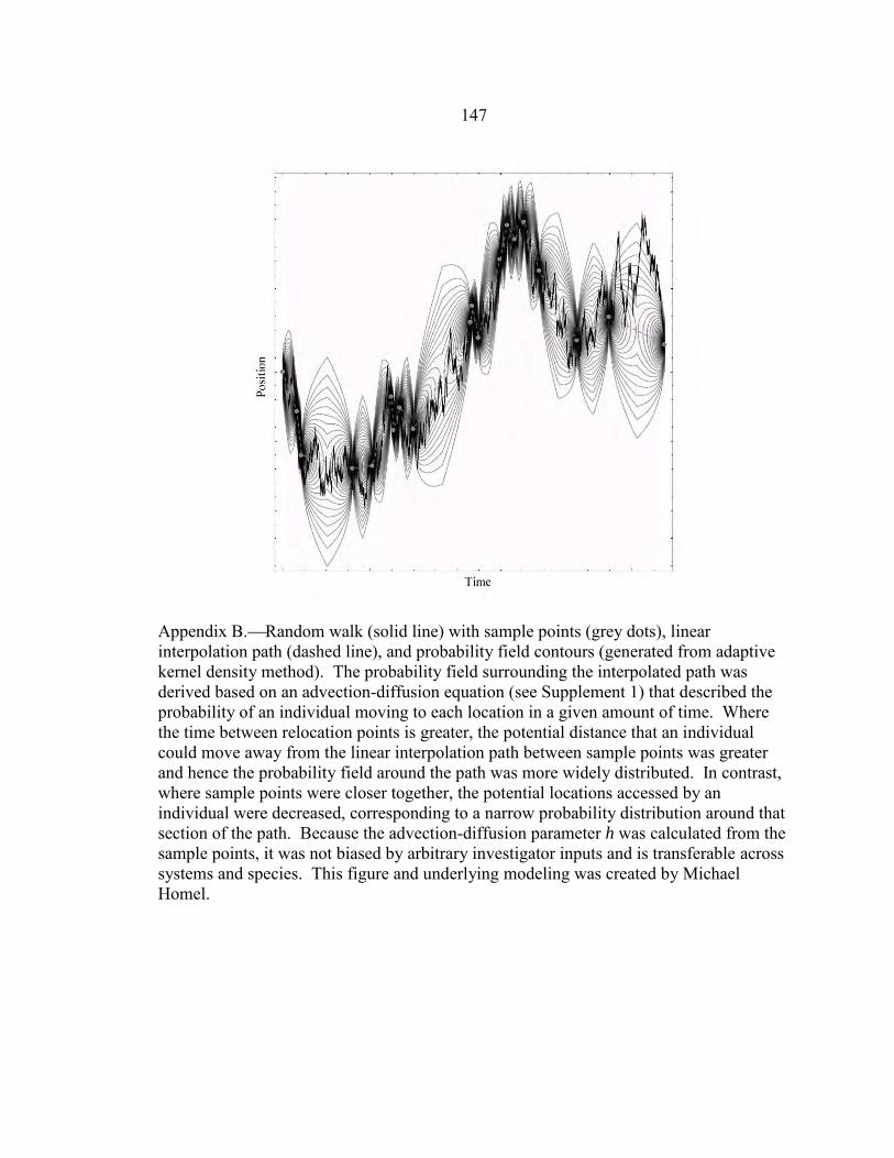
147
Appendix B.Random walk (solid line) with sample points (grey dots), linear interpolation path (dashed line), and probability field contours (generated from adaptive kernel density method). The probability field surrounding the interpolated path was derived based on an advection-diffusion equation (see Supplement 1) that described the probability of an individual moving to each location in a given amount of time. Where the time between relocation points is greater, the potential distance that an individual could move away from the linear interpolation path between sample points was greater and hence the probability field around the path was more widely distributed. In contrast, where sample points were closer together, the potential locations accessed by an individual were decreased, corresponding to a narrow probability distribution around that section of the path. Because the advection-diffusion parameter h was calculated from the sample points, it was not biased by arbitrary investigator inputs and is transferable across systems and species. This figure and underlying modeling was created by Michael Homel.

148
APPENDIX C
ANNOTATED CODE (CREATED BY MICHAEL HOMEL USING THE PROGRAM MATHEMATICA) FOR EACH INTERPOLATION METHOD, RANDOM-WALK
SIMULATIONS, AND METHOD COMPARISON

149

150

151

152

153

154

155

156

157

158

159

160

161

162

163
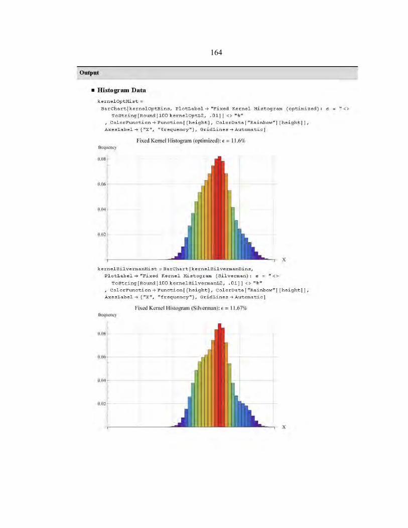
164

165

166

167

168

169

170
\
APPENDIX D
ANNOTATED MODEL CODE (CREATED BY MICHAEL HOMEL USING PROGRAM MATHEMATICA) FOR APPLYING THE ADAPTIVE KERNEL
DENSITY INTERPOLATION METHOD TO AN ACTUAL DATASET

171
Input relocation data need to take the form of column 1 = individual location (e.g., in river meters) and column 2 = time (e.g., in day of study, not calendar date) without any headings. Data must be sorted by individuals and ordered temporally. Once data are imported into Mathematica, the dataset needs to be split into smaller sets corresponding to the line numbers that encompass the relocations of a single individual. The spatial scale of the data should correspond to a reasonable temporal scale (e.g., meters and hours or kilometers and days) and the code is currently programmed to convert data in meters into kilometers. Spatial binning into geomorphic reaches can be easily accomplished by creating a spreadsheet with the reach identifier in column1 and the river meter location at the bottom of each reach in column 2.

172

173

174

175

176

177

178
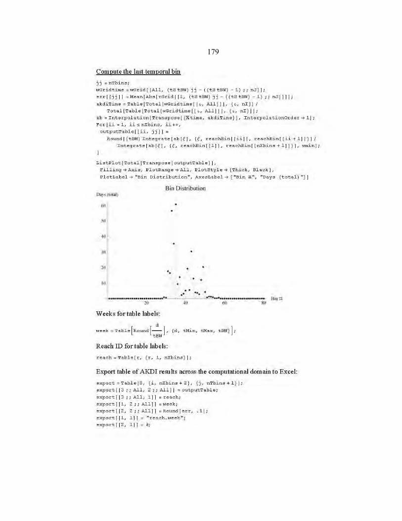
179

180

181