spatial dynamics and convergence: the spatial ak model
TRANSCRIPT

Spatial dynamics and convergence: The spatial AK
model
R. Boucekkine∗, C. Camacho†, G. Fabbri‡.
March 18, 2010
Abstract
We study the optimal dynamics of an AK economy where popu-lation is uniformly distributed along the unit circle. Locations onlydiffer in initial capital endowments. Despite constant returns to cap-ital, we prove that transition dynamics will set in. In particular, weprove that the spatio-temporal dynamics, induced by the willingnessof the planner to give the same (detrended) consumption over spaceand time, lead to convergence in the level of capital across locations inthe long-run.
JEL Classification: C60, O11, R11, R12, R13.Keywords: Economic Growth, Inequality, Spatial Dynamics, Conver-gence.
∗Department of Economics and CORE, Universite catholique de Louvain, Louvain-La-Neuve, Belgium; Department of Economics, University of Glasgow, Scotland. E-mail:[email protected]
†Belgium National Fund for Research, FNRS and Department of Eco-nomics, Universite catholique de Louvain, Louvain-La-Neuve, Belgium. E-mail:[email protected]
‡Dipartimento di Studi Economici S. Vinci, Universita di Napoli Parthenope, Naples,Italy and IRES, Universite catholique de Louvain, Louvain-La-Neuve, Belgium. E-mail:[email protected]
aWe acknowledge fruitful discussions with Stefano Bosi, Thomas Seegmuller and Ben-teng Zou. R.Boucekkine and C. Camacho are supported by a grant from the BelgianFrench-speaking Community (convention ARC 09/14-018 on Sustainability.)
1

1 Introduction
The issue of optimal and market allocation of economic activity across spacehas always been a central issue in economic theory from the seminal works ofHotelling (1929) and Salop (1979). Many authors have already investigatedin depth the existence (and sometimes the non-existence) of optimal and/ormarket allocation in static models (among them, Starrett, 1974 and 1978).Recently, some authors have tried to tackle the issue of the spatial alloca-tion of economic activity in dynamic frameworks, namely within economicgrowth frameworks (thus, with capital accumulation). This research line,initiated by Brito (2004), is nicely surveyed by Desmet and Rossi-Hansberg(2010). Two aspects turn out to be crucial: factor mobility and space mod-elling. On the first aspect, Brito and Boucekkine, Camacho and Zou (2009)consider frictionless capital mobility while Brock and Xepapadeas (2008) usethe trick of a spatial externality to model the spatial component (withoutcapital mobility). In the former papers, the production function at any placeis neoclassical (decreasing returns in capital): capital flow from regions withlow marginal productivity of capital to regions with high marginal produc-tivity.
Concerning spatial modelling, both Brito and Boucekkine et al. consideran infinite spatial line, symmetrical to the infinite time horizon adopted instandard growth theory. But while Boucekkine et al. introduce spatial dis-counting (again mimicking time discounting) to ensure the convergence ofthe resulting utilitarian objective function, Brito postulates a non-utilitarianobjective function and gets rid of spatial discounting. Brock and Xepapadeas(2008) take a compact interval to model space, therefore avoiding this tech-nical problem. A striking finding of Boucekkine et al. is that the modelwith infinite time and space support, and utilitarian objective function withstrictly concave preferences, which is admittedly the most natural candidatefor spatial Ramsey model, suffers from a structural ill-posedness problem:in contrast to the non-spatial Ramsey model, the initial value of the co-statevariable is no longer sufficient to determine the optimal paths. Rather thanconsidering a non-standard objective function as in Brito (2004), we fol-low here the example of Brock and Xepapadeas (2008) and consider a morerealistic compact modelling of space. However, in sharp contrast to theseauthors, we do not consider a compact interval on the real line but a circle,which is another traditional modelling of space in economics (Salop, 1979).A very important advantage of our modelling is that it does not require thespecification of any space boundary conditions, to which the solution paths
2

are arguably extremely sensitive. We also keep capital mobility in line withBoucekkine et al. (2009).
In order to gather at least some partial clean analytical results, wewill consider an AK technology. Using recent developments in dynamicprogramming in infinitely-dimensioned problems (Bensoussan et al., 2007),previously implemented in the literature of vintage capital theory (Fabbriand Gozzi, 2008), it is possible to identify an explicit value function underquite reasonable parametric conditions. As in the standard AK model, abenevolent social planner will choose a constant consumption level (that isdetrended consumption): in our spatial set-up, this turns out to be truenot only over time but also over space assuming homogeneous preferencesand technology over space. Also, we will show that the aggregate capitalstock, that’s the aggregation of capital stocks across space, lies on a balancedgrowth path from t = 0, featuring the absence of transitional dynamics forthe aggregate variables as in the standard AK theory. A major and strik-ing departure from the standard theory will nonetheless emerge: while theaggregate capital stock shows no dynamics, an intense reallocation of cap-ital will take place across space giving rise to transition dynamics at anypoint in space. Even more strikingly, these spatio-temporal dynamics willlead to the convergence of (time detrended) capital stocks across space tothe same common value whatever the initial spatial distribution of capitalunder certain realistic assumptions.
Two crucial points should be made here. First of all, the spatial dynam-ics generated in the AK case are essentially different from those exhibited inBoucekkine et al.: in the former, there are no decreasing returns to capital,and the whole dynamics derive from the will of the benevolent planner tokeep consumption level constant over time and space, and to move capitalaccordingly. Second, the similarity between the AK vintage model (as stud-ied initially in Boucekkine et al., 2005, and revisited by Fabbri and Gozzi,2008) and the AK spatial model should be noted here: in both, capital hasa double heterogeneity (time and vintage in the vintage AK model, andtime and space in the spatial AK), resulting in finitely-dimensioned optimalcontrol problems; in both detrended consumption is constant, and capitaltransition dynamics emerge.
This said, the spatial modelling adopted in this paper allows to get muchmore specific and striking results concerning the property of economic con-vergence as outlined above. In our setting, returns to capital are constant,and one would not take for granted convergence of capital stocks over space,
3

that’s transition dynamics equalizing capital across space. Typically, de-creasing returns to capital are invoked as the engine of convergence in theneoclassical growth model. Things are much more involved if one keepsin mind that in our framework initial capital stock is heterogenous acrossspace, which could be at first glance related to the literature of growth withheterogenous initial endowments (initiated by Stiglitz, 1969, and pushedforward by Chatterjee, 1994).a In this literature, decreasing returns to cap-ital are not enough to ensure convergence of wealth across individuals: ifthey differ only in their initial endowments and share the same homotheticpreferences, initial inequalities will be reproduced for ever! In a sense, ourpaper establishes a kind of symmetric property: convergence is obtainedunder constant return to capital. This said, one should not omit the specificnature of spatial dynamics. Among other specific results, we analyticallyshow that convergence of capital stocks across space is guaranteed when thetime discount rate is not to big, a requirement which does not appear in thegrowth literature with heterogenous endowments.
The paper is organized as follows. Section 2 sketches the model. Section3 displays the analytical results. Section 4 provides some numerical illus-trations and exercises regarding the convergence and divergence questionsoutlined above. Section 5 concludes.b
2 The model
We first present the law of motion of capital in time and space. Weshall follow here the very generic modelling adopted in the related literature(as recently re-used by Boucekkine et al., 2009). At a given point (t, x) ∈[0,∞) × R, physical capital k(t, x) evolves according to
∂k
∂t(t, x) = Ak(t, x) − c(t, x) − τ(t, x). (1)
A represents the level of technology, which we assume to be constant overtime and space. The production function is AK at any point in space. c(t, x)and τ(t, x) stand respectively for consumption and trade balance at the tradebalance at (t, x) ∈ [0,∞) × R. Capital depreciation is zero everywhere.Finally, we assume that there is no adjustment or transportation cost whenmoving capital from a location to another. Such costs traditionally generate
aSee also Caselli and Ventura (2000) for a more recent contribution.bWe report the heavy mathematical apparatus needed to solve the model in the ap-
pendix.
4

non-instantaneous adjustment (to the optimal outcomes), we switch off thisdynamics engine in this model to only rely on spatial dynamics (if any).
Now we come to the space modelling. We assume that individuals aredistributed homogeneously along the unit circle, which we denote by T:
T :=
x ∈ R2 : |x| = 1
Two remarks are in order here. First of all, our assumption of a non-growing and spatially homogeneous population distribution is made forconvenience. Considering an heterogenous spatial population distributionwould lead to introduce space weights in the objective social welfare func-tion, which will break down the simple analytical solution derived in thispaper. We prefer sticking to our analytical case for clarity. Second, as ar-gued in the introduction section, the choice of the unit circle to representspace is not innocuous, it allows to avoid the specification of boundary con-ditions, which use to condition decisively the shape of optimal dynamics.It is worth mentioning here that the results obtained along this paper arerobust to certain modifications of the space geometry. More precisely, wecan study the problem on a more general n-dimensional compact and con-nected manifold without boundary but the mathematical apparatus has tobe adapted accordingly.c
Let us focus on the trade balance in region B, an arc of the circle. Wehave that
∫
B
τ(t, x) dx =∂k
∂x(t, b) −
∂k
∂x(t, a),
the regional trade balance is equal to the capital entering from one or itsborders less the capital flowing away from the other border. Using theFundamental Theorem of Calculus we can rewrite the above expression as
∫
B
τ(t, x) dx =
∫
B
∂2k
∂x2(t, x) dx. (2)
Hence the following equality holds in region B:
∫
B
(
∂k
∂t(t, x) −
∂2k
∂x2(t, x) − Ak(t, x) + c(t, x)
)
dx = 0. (3)
The evolution of physical capital at any point (t, x) ∈ R+ × B is obtained
using (3) when the length of B tends to zero, for any B arc of T. Provided
cIn this more general setting the Laplace operator on T considered here has to bereplaced by the so-called Laplace-Beltrami operator on the manifold.
5
an initial distribution of physical capital k0(·) on T , the policy maker hasto choose a control c(·, ·) to maximize the following functional
maxc(·,·)
J(k0, c(·, ·)) :=
∫ +∞
0e−ρt
∫
T
(c(t, x))1−σ
1 − σdxdt. (4)
subject to the state equation
∂k
∂t(t, x) =
∂2k
∂x2(t, x) + Ak(t, x) − c(t, x)
k(t, 0) = k(t, 2π)k(0, x) = k0(x).
(5)
We define Uk0 as the set of admissible controls for the problem (4)-(5), whichdepends on the initial distribution k0:
Uk0 :=
c(·, ·) ∈ L2(R+ × T; R+) : k(t, x) ≥ 0 for all (t, x) ∈ R+ × T
(6)The value function of our problem starting from k0 is defined as
V (k0) := supc(·,·)∈Uk0
J(k0, c(·, ·))
A few comments are in order here. In first place, it should be notedthat the social welfare objective function considered “treats” equally allthe individuals independently of their location, that is independently oftheir initial capital endowment. One would invoke ethical criteria to justifya spatially-weighted objective function, for example to account for initialinequalities. Here we show that without this kind of weighting, capitalstocks will end up equalized across space. It should be also noted that weconcentrate here on planner’s optimal solutions, we do not address the issueof decentralization, which would probably bring us close to consider spatialweighting in the spirit of Negishi (1960). The next section is devoted touncover the main analytical properties of our central planner problem.
3 Spatial dynamics in the AK model: analytical
results
We shall start by characterizing a crucial property of the optimal solution:As in the pre-exiting AK frameworks (with or without vintage capital), theplanner will choose a constant consumption level over time and space, and
6

all aggregate variables will grow at a constant growth rate from t = 0. Thenext proposition establishes the existence of a unique explicit value functionand gives a first characterization of optimal consumption.
Theorem 3.1. Suppose that
A(1 − σ) < ρ (7)
and consider k0 ∈ L2(T) a positive initial distribution of physical capital.Define
η :=ρ − A(1 − σ)
2πσ. (8)
Provided that the trajectory k∗(t, x) driven by the feedback control (constantin x)
c∗(t, x) = η
∫
T
k∗(t, y) dy (9)
remains positive,d c∗(t, x) is the unique optimal control of the problem.Moreover the value function of the problem is finite and can be written ex-plicitly as
V (k0) = α
(∫
T
k0(x) dx
)1−σ
(11)
where
α =1
1 − σ
(
ρ − A(1 − σ)
2πσ
)−σ
. (12)
Proof. See Appendix B.
The theorem deserves some comments. First of all, the parametric condi-tion (7) is exactly the one needed in the counterpart standard AK theory toassure that the objective function is finite (or equivalently, that the transver-sality condition is met). It is also needed here to guarantee that the valuefunction of the problem is finite. The value function V (k0) is given explicitlyby (11): notice that it depends only on the aggregate initial capital stock.Two different capital distributions will give the same value function, and
dThe trajectory driven by the feedback control is the unique solution of
∂k(t, x)
∂t= ∂2
xk(t, x) + Ak(t, x) − η
∫
T
k(t, y) dy
k(t, 0) = k(t, 2π)
k(0, x) = k0(x).
(10)
7
therefore the same optimal consumption rule (here given by equation (9)):the optimal solution features therefore a kind of pooling of resources, whichis hardly surprising given the social optimum framework considered here.Finally, one has to notice that both the value function and the feedbackcontrol are similar to those of the standard AK model. However, the pro-portionality parameters η and α are specific to the space modelling adoptedin this paper. We now extract the optimal solutions for the aggregate capitalstock and the induced optimal consumption rule at any point (t, x).
Proposition 3.2. Under the same assumptions of Theorem 3.1 the aggre-gate capital K(t) :=
∫
Tk(t, y) dy, along the optimal trajectories, is
K(t) = K(0)eβt (13)
where
β :=
[
A − ρ
σ
]
. (14)
and K(0) :=∫
Tk0(y) dy.
Proof. See Appendix B.
Notice that the optimal aggregate capital stock evolves exactly as in thestandard AK model: it grows at the same standard growth rate, β = A−ρ
σ,
from t = 0. From (7), one can then use (13) to obtain that the optimal con-trol is c∗(t, x) = ηK(0)eβt. As announced repeatedly above, we obtain thecrucial property that the planner will choose the same (detrended) consump-tion level for all individuals whatever their location and generation. Thus,the aggregate variables have no transition dynamics just like in the stan-dard AK theory. Nonetheless, if the planner is willing to keep (detrended)consumption constant over time and space, he has to move capital over timeand space accordingly. What could be the induced optimal spatio-temporaldynamics? The next theorem gives the answer to this appealing question.Indeed, once we obtain an explicit solution for the optimal choice of thepolicy maker, we can replace it into (5) to study the evolution of physi-cal capital. This can be done explicitly in our setting under an additionalparametric condition.
Theorem 3.3. Assume that the hypotheses of Theorem 3.1 are satisfied.Suppose that
ρ < A(1 − σ) + σ. (15)
8

Then, along the optimal trajectory, the detrended capital
kD(t, x) :=k(t, x)
eβt(16)
converges uniformly (and a fortiori pointwise), as a function of x, to the
constant function K(0)2π
when t tends to infinity. In other words
limt→∞
(
supx∈T
∣
∣
∣
∣
kD(t, x) −K(0)
2π
∣
∣
∣
∣
)
= 0.
Proof. See Appendix B.
Theorem 3.3 is the main result of this paper: it shows that the spatio-temporal dynamics induced by the willingness of the planner to give the same(detrended) consumption over space and time lead to equalize the capitallevel across locations in the long-run. Hence, spatio-temporal dynamics doeliminate the initial inequalities in capital endowments in our spatial AKmodel. As mentioned in the introduction, this result is striking in many re-spects, notably with respect to the traditional theory of convergence, whichtypically builds on representative agents settings. In the latter, decreasingreturns to capital drive convergence while AK technologies are associatedwith divergence (due to the absence of transition dynamics). If one has inmind the existing (rather thin) literature on the link between growth andinequalities where individuals have heterogenous initial endowments, thenour result could be interpreted at first glance as symmetrical to the tradi-tional property highlighted by Chatterjee (1994): under decreasing returnsto capital, initial inequalities will be reproduced for ever. This said, thespatial dynamics entailed in our model are specific (though they derive froma generic law of motion of capital in space and time). In particular, our con-vergence result is guaranteed when ρ < A(1−σ)+σ. Otherwise, everythingcan happen. Notice however, that this condition is very largely satisfiedin realistic parameterizations of the model. The next section provides acomplementary numerical investigation.
9

4 Spatial dynamics in the AK model: computa-
tional results
We perform a numerical exercise to shed more light on the transitionaldynamics of the spatial AK-modele. We use the isomorphism between thecircumference T and the closed interval [0, 2π] once we have identified thetwo boundary points 0 and 2π. There are three parameters key to ourmodelling, ρ, A and σ. In the Ak-model, A = Y/k and consequently wechoose A = 1/3 as a reasonable ratio output to physical capital. Then wefix ρ = 0.07 and σ = 0.8, the set ρ,A, σ satisfies both (7) and (15).
Table 1: Parameters values
Total Factor Productivity A 1/3Time discount rate ρ 0.07Intertemporal elasticity of substitution σ 0.8
Provided that conditions (7) and (15) holdf, Theorem 3.3 proves that
detrended capital at any point (t, x) converges to the constant function K(0)2π
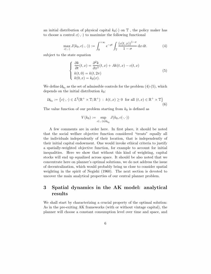
when t tends to infinity. To illustrate this result, we study the case of aneconomy made of two regions, the first region, [0, π] is initially endowed withtwice the capital of the second region, [π, 2π], namely
k0(x) =
20, x ∈ [0, π],10, x ∈ [π, 2π].
Theorem 3.3 shows that the policy maker allocates the same amount ofconsumption to all locations x at any time t. In the standard Ak-model theoptimal trajectory instantaneously adjusts to the optimal consumption andproduction plan. This behavior does no longer hold when physical capital isallowed to move across space as figures 1 and 2 show. Capital moves from
eProvided that conditions (7) and (15) hold, the optimal trajectory of physical capitalcan be simulated using the Fourier series of kD:
kD(t, x) =K(0)
2π+∑
n∈N
n6=0
e(A−n2−β)t
√π
(
cos(nx)
∫
T
k0(x) cos(nx)dx + sin(nx)
∫
T
k0(x) sin(nx)dx
)
For our exercise n = 20.fFor A = 1/3 and σ = 0.8, the range of values for ρ which satisfies conditions (7) and
(15) is ]0.0667, 0.8667[.
10

rich locations towards poor ones, but adjustment is not instantaneous sinceit takes time for capital to achieve its final location. As capital moves awave appears and it brings about the emergence of a temporary productionagglomeration in the rich region. Simultaneously, a depressed area is formedin the center of the poor region. When capital moves from left to right, alllocations in the rich region send capital to the poor region to reach theoptimal path. The depressed area appears since capital moves from t = 0and from left to right, also within the poor region, without waiting for thelocations to achieve a level close to optimal to pass capital. With time,both the agglomeration and depression lose force and we can observe acomplete convergence to the spatially homogenous steady state value fordetrended capital from t = 10. The graphs show physical capital acrossspace at different moments: on the top panel of figure 1 at times t = 0.02,t = 0.2, t = 1 and t = 10. The bottom panel shows the optimal trajectoryof detrended physical capital for (x, t) ∈ [0, 2π] × [0, 8]g.
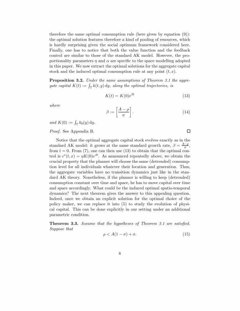
Figure 2 illustrates the importance of condition (15). For this exampleρ = A(1−) + σ = 0.8667 and we can see that detrended capital does notconverge to an spatially homogenous distribution. A noteworthy aspect isthat detrended physical capital does converge to a steady state, and it doesso very fast.
gConvergence towards the steady state would have been slower if transportation costs,adjustment costs, capital depreciation or trade barriers had been present.
11

0 1 2 3 4 5 65
10
15
20
25
Space from 0 to 2π
k
t = 0.02
t = 0.2
t = 1
t = 10
02
46
810
01
23
45
6
5
10
15
20
25
TimeSpace
Figure 1: On the top panel: physical capital distribution at t = 0.02, 0.2, 1, 10.The bottom panel shows k(t, x) where (t, x) ∈ [0, 8]× [0, 2π].
12

0 1 2 3 4 5 60
5
10
15
20
25
30
Space from 0 to 2π
k
t = 0.02
t = 0.2
t = 1
t = 10
02
46
810
01
23
45
60
5
10
15
20
25
30
TimeSpace
Figure 2: On the top panel: physical capital distribution at t = 0.02, 0.2, 1, 10.The bottom panel shows k(t, x) where (t, x) ∈ [0, 8]× [0, 2π].
13

5 Concluding remarks
In this paper, we have shown how spatial dynamics, introduced through ageneric law of motion of capital, interact with the mechanics inherent to theAK model. The main result of our work is that the spatio-temporal dynam-ics, induced by the willingness of the planner to give the same (detrended)consumption over space and time, lead to convergence in the level of capitalacross locations in the long-run. An important opened line of research is tostudy to which extent our results are robust to the introduction of spatialweights in the objective function to cope with specific ethical criteria. An-other one, more ambitious, would address decentralization in an attempt toextend Negishi’s work to this type of spatial models.
References
[1] A. Bensoussan, G. Da Prato, M.C. Delfour and S.K. Mitter. Repre-sentation and control of infinite dimensional system. Second edition.Birkhauser, Boston, 2007.
[2] R. Boucekkine, O. Licandro, L. Puch and F. del Rıo. Vintage capitaland the dynamics of the AK model. Journal of Economic Theory 120,39-76 (2005).
[3] R. Boucekkine, C. Camacho and B. Zou. Bridging the gap betweengrowth theory and the new economic geography: the spatial Ramseymodel. Macroeconomic Dynamics 13, 20-45 (2009).
[4] P. Brito. The dynamics of growth and distribution in a spatially het-erogenous world. WP 13/2004, ISEG Working Papers (2004).
[5] W. Brock and A. Xepapadeas. General pattern formation in recursivedynamical systems in economics. MPRA paper 12305 (2008).
[6] F. Caselli and J. Ventura. A representative consumer theory of distribu-tion. The American Economic Review 90, 909-926 (2000).
[7] S. Chatterjee. Transitional dynamics and the distribution of wealth ina neoclassical growth model. Journal of Public Economics 54, 97-119(1994).
[8] K. Desmet and E. Rossi-Hansberg. On spatial dynamics. The Journal ofRegional Science 50, 43-63 (2010).
14

[9] G. Fabbri and F. Gozzi. Solving optimal growth models with vintage cap-ital: The dynamic programming approach. Journal of Economic Theory143, 331-373 (2008).
[10] H. Hotelling. Stability in competition. Economic Journal xxxix, 41-57(1929).
[11] T. Negishi. Welfare economics and existence of an equilibrium for acompetitive equilibrium. Metroeconomica 12, 92-7 (1960).
[12] S.Salop. Monopolistic competition with outside goods. Bell Journal ofEconomics 10, 141-156 (1979).
[13] D. Starrett. Market allocations of location choice in a model with freemobility. Journal of Economic Theory 17, 21-37 (1978)
[14] D. Starrett. Principles of optimal location in a large homogenous region.Journal of Economic Theory 9, 418-448 (1974).
[15] J. Stiglitz. Distribution of income and wealth among individuals. Econo-metrica 37, 382-397 (1969).
15

Appendices
A The Hilbert space setting
Consider the Hilbert space L2(T) and define the operator
D(G) := H2(T)G(f) = ∆f.
G is the generator of the C0-semigroup etG (the heat semigroup) on L2(T). Theoperator G is self-adjoint (so D(G∗) = D(G) and G∗φ = Gφ = ∆φ). The stateequation (5) can be rewritten as an evolution equation in L2(T)
k(t) = Gk(t) + Ak(t) − c(t)k(0) = k0.
(17)
With an abuse of the notation we denote by k(·) the solution of (17). Thisis justified by the fact that k(t)(x) = k(t, x) where the latter is the solutionof (5). The set of the admissible controls in the infinite dimensional setting is
c ∈ L2(
R+; L2(T; R+)
)
: k(t)(x) ≥ 0 for all (t, x)
. It is exactly equivalent tothe set Uk0
defined in (6) so the abuse of the notation “c” is justified too. The mildform of (17) is
k(t) = eGtk0 +
∫ t
0
e(t−s)G (Ak(s) − c(s)) ds.
Let us denote by 〈·, ·〉 the scalar product on L2(T) and by 1 the function
1 : T → R1(x) ≡ 1.
Note that 1 ∈ D(G). Using such a notation the functional (4) can be rewritten as
∫ +∞
0
e−ρt 〈1, U(c(t))〉 dt
where, for a given η ∈ L2(T), U(η) : T → R is the function U(η) : x 7→ (η(x))1−σ
1−σ .
The Hamilton-Jacobi-Bellman equation (HJB equation hereafter) of the system isdefined as
ρv(k) = 〈k, G∇v(k)〉 + A 〈k,∇v(k)〉 + supc∈L2(T;R+)
− 〈c,∇v(k)〉 + 〈1, U(c)〉 . (18)
B Proofs
This sections contains the proofs of the theorems and of the propositions presentedin the text. We use the setting and the notation introduced in Appendix A. The
16

statement of the theorems in Section 3 are formulated, for the reader convenience,without using the infinite dimensional language (we used there the PDE formalism),but, of course, they are completely equivalent to the related infinite-dimensionalones we present here.
Proof of Theorem 3.1. We prove the theorem using the dynamic programming.The proof is presented in some steps:
Step 1: We find an explicit solutionh of the HJB equation (18) on the open setΩ :=
k ∈ L2(T) : 〈k,1〉 > 0
.
We look for a solution of (18) of the following form: v(k) = α 〈k,1〉1−σfor
some positive real number α, so that ∇v(k) = α(1 − σ) 〈k,1〉−σ 1. Note that, forall k ∈ Ω, ∇v(k) ∈ D(G) and that ∇v : Ω → D(G) is continuous (when D(G) isendowed with the graph norm). Substituting in (18) we obtain:
ρα 〈k,1〉1−σ = α(1 − σ) 〈k,1〉−σ 〈k, G1〉 + Aα(1 − σ) 〈k,1〉−σ 〈k,1〉+ sup
c∈L2(T;R+)
−α(1 − σ) 〈k,1〉−σ〈c,1〉 + 〈1, U(c)〉
.
Observing that G1 = 0 and that the supremum is attained when c =
(α(1 − σ))−1/σ
〈k,1〉1 the expression above becomes:
ρα 〈k,1〉1−σ= Aα(1 − σ) 〈k,1〉1−σ
− 2πα(1 − σ) (α(1 − σ))−1/σ
〈k,1〉1−σ+ 2π
[
(α(1 − σ))−1/σ 〈k,1〉]1−σ
1 − σ. (19)
From (19) we have
ρ = A(1 − σ) − 2π(1 − σ) (α(1 − σ))−1/σ
+ 2π (α(1 − σ))−1/σ
so there exists a solution of the requested form when
α =1
1 − σ
(
ρ − A(1 − σ)
2πσ
)−σ
.
Before passing to step 2 we make an observation that will be useful later: givenan admissible (and hence positive) control c(·), the related trajectory k(·) is given bythe solution of (17). Therefore at every time and at every point x of the space k(·)
remains below the solution of ˙k(t) = Gk(t) + Ak(t) with k(0) = k0. In particular,
hWe say that v from some open set O in L2(T) to R is a solution (on O) of (18) ifv ∈ C1(O; D(G)) (where D(G) is endowed with the graph norm) and v solves (18) atevery point of O.
17

for all t ≥ 0,⟨
k(t),1⟩ ≥ 〈k(t),1〉. k(t) can be expressed as k(t) = etAetGk0 so that⟨
k(t),1⟩ = etA⟨
k0,1⟩. This means that for every choice of c(·) we have
∣
∣e−ρtv(k(t))∣
∣ = e−ρtα 〈k(t),1〉1−σ≤ e−ρtα
⟨
k(t),1⟩1−σ
= e−ρtetA(1−σ)⟨
k0,1⟩ = e−(ρ−A(1−σ)t)⟨
k0,1⟩ t→∞−−−→ 0 (20)
where we obtain the last limit thanks to Hypothesis (7).
Step 2: We prove that the feedback control provided by the solution is admissible.The feedback control provided by the solution is
φ : L2(T) → L2(T)
φ(k) := arg maxc∈L2(T)
−α(1 − σ) 〈k,1〉−σ〈c,1〉 + 〈1, U(c)〉
=
= (α(1 − σ))−1/σ 〈k,1〉1 = η 〈k,1〉1 (21)
where η = ρ−A(1−σ)2πσ , the related trajectory is the solution of the mild equation
k(t) = eGtk0 +
∫ t
0
e(t−s)G (Ak(s) − η 〈k,1〉1) ds. (22)
Proving that such an equation has a unique solution k∗(t) and that k∗(t)(x) =k∗(t, x) where k∗(t, x) is the solution of (10) are standard facts (see for exampleBensoussan et al. (2007) ). The control we want to prove to be admissible (and thatwe prove to be optimal in step 3) is that defined, for all t ≥ 0, as c∗(t) := φ(k∗(t)).Since by hypothesis k∗(t)(x) remains positive, then c∗(t) remains positive too andthen it is admissible.
Step 3: We prove that the feedback control provided by the solution is optimal(proving at the same time that the solution of the HJB equation we found is indeedthe value function).
To prove that c∗(·) is an optimal control we have to prove that for every otheradmissible control c(·) we have J(k0, c
∗(·)) ≥ J(k0, c(·)).Let us call k(·) the trajectory related to the admissible control c(·) and let us
denote by w(t, k) : R × L2(T) → R the function w(t, k) := e−ρtv(k). We have:
v(k0) − w(T, k(T )) = w(t, k(0)) − w(T, k(T )) = −
∫ T
0
d
dtw(t, k(t)) dt
=
∫ T
0
e−ρt[
ρv(k(t)) −⟨
Gk(t) + Ak(t) − c(t),∇v(k(t))⟩]
dt
The last expression makes sense thanks to the regularizing properties of the heatsemigroup (in particular for all t > 0, k(t) ∈ D(G)). Passing to the limit in the lastexpression, as t → ∞, (using (20)) we have
v(k0) =
∫ +∞
0
e−ρt[
ρv(k(t)) −⟨
Ak(t) − c(t),∇v(k(t))⟩
−⟨
k(t), G∇v(k(t))⟩]
dt
18

and then
v(k0) − J(k0, c(·))
=
∫ +∞
0
e−ρt
[(
ρv(k(t)) −⟨
Ak(t),∇v(k(t))⟩
−⟨
k(t), G∇v(k(t))⟩
)
+
(
⟨
c(t),∇v(k(t))⟩
− 〈1, U(c(t))〉
)]
dt
=
∫ +∞
0
e−ρt
[
(
supc∈L2(T;R+)
−⟨
c,∇v(k(t))⟩
+ 〈1, U(c)〉
)
−(
−⟨
c(t),∇v(k(t))⟩
+ 〈1, U(c(t))〉)
]
dt ≥ 0.
We used the fact that v is a solution of (18). Last expression gives v(k0) −J(k0, c(·)) ≥ 0 and from the same expression we can also easily see thatv(k0) − J(k0, c
∗(·)) = 0 (indeed c∗(·) is defined using the feedback defined in(21)). So, for all admissible c, v(k0) − J(k0, c(·)) ≥ 0 = v(k0) − J(k0, c
∗(·))and then J(k0, c(·)) ≤ J(k0, c
∗(·)) and then c∗ is optimal. In particular, sincev(k0) = J(k0, c
∗(·)) = 0 and c∗ is an optimal control, v(k0) is the value func-tion at k0. The uniqueness of the optimal control follows from standard convexityconsiderations.
Proof of Proposition 3.2. Along the optimal trajectories we have
k(t) = eGtk0 +
∫ t
0
e(t−s)G (Ak(s) − c(s)) ds
= eGtk0 +
∫ t
0
e(t−s)G (Ak(s) − η 〈k(s),1〉 1) ds. (23)
so
K(t) = 〈k(t),1〉 =⟨
k0, eGt1⟩+
∫ t
0
⟨
(Ak(s) − η 〈k(s),1〉 1) , e(t−s)G1⟩ ds
where we used that etG is self-adjoint. Moreover using that eGt1 = 1 the expressionabove becomes:
= K(0) +
∫ t
0
K(s)
[
A − 2πρ − A(1 − σ)
2πσ
]
ds = K(0) +
∫ t
0
K(s)
[
A − ρ
σ
]
ds.
So K(t) has to be equal to K(0)eβt where β = (A−ρ)/σ and the claim is proved.
Proof of Theorem 3.3. We begin showing that kD(t) converges to K(0)12π in the
L2(T) norm when t → +∞. We write kD(t, x) using Fourier series. For n ∈ Z, we
19

call en the function en : T → R given by
en(x) :=
cos(nx)√π
if n ≥ 1sin(−nx)√
π= sin(nx)√
πif n ≤ −1
1√2π
if n = 0.
They are a complete orthonormal Hilbert basis of L2(T). Consider the selfadjointoperator G on L2(T)
G := G + A
having the same domain of G. Equation (23) can be written in the followingequivalent form:
k(t) = eGtk0 −
∫ t
0
e(t−s)Gη 〈k(s),1〉1 ds.
The Fourier coefficients can be found using such an expression:
〈kD(t), en〉 = e−βt 〈k(t), en〉
= e−βt⟨
eGtk0, en
⟩
− e−βt
∫ t
0
⟨
e(t−s)Gη 〈k(s),1〉1, en
⟩
ds
= e−βt⟨
k0, eGten
⟩
− e−βt
∫ t
0
η 〈k(s),1〉⟨1, e(t−s)Gen
⟩
ds, (24)
using that eGten = e(−n2+A)ten and that, for n 6= 0, 〈en,1〉 = 0, we can see that
〈kD(t), en〉 = e−βt⟨
k0, e(A−n2)ten
⟩
= e(A−n2−β)t 〈k0, en〉 , n 6= 0
If n = 0 we have 〈kD(t), e0〉 = K(0)√2π
(it follows immediately from Proposition
3.2). Let us we prove now that kD(t) converges in the L2-norm to K(0)12π : consider
ε ∈(
0, A(1−σ)+σ−ρσ
)
(it exists thanks to (15)) we have
∣
∣
∣
∣
kD(t) −K(0)1
2π
∣
∣
∣
∣
2
L2(T)
=∑
n∈Z
⟨(
kD(t) −K(0)1
2π
)
, en
⟩2
=∑
n∈Z
n6=0
e2(A−n2−β)t 〈k0, en〉2
= e−2εt∑
n∈Z
n6=0
e2(A−n2−β+ε)t 〈k0, en〉2
≤ e−2εt∑
n∈Z
n6=0
〈k0, en〉2≤ e−2εt |k0|
2L2(T)
t→∞−−−→ 0,
where we used that, for all n 6= 0, (A − n2 − β + ε) < 0. Observe now that theFourier series of k(t)
kD(t)[x] =K(0)
2π+∑
n∈Z
n6=0
e(A−n2−β)t 〈k0, en〉 en[x] (25)
20

converges uniformly for t > 0 so kD(t)[·] ∈ C(T) and
supx∈T
∣
∣
∣
∣
kD(t)[x] −K(0)
2π
∣
∣
∣
∣
= supx∈T
∣
∣
∣
∣
∣
∣
∣
∑
n∈Z
n6=0
e(A−n2−β)t 〈k0, en〉 en[x]
∣
∣
∣
∣
∣
∣
∣
≤ e−εt
∣
∣
∣
∣
∣
∑
n∈Z
e(A−n2−β+ε)t|k0|L2 supx∈T
|en[x]|
∣
∣
∣
∣
∣
≤ |k0|L2e−εt∑
n∈Z
e(A−n2−β+ε)t. (26)
Considering t ≥ 1 and calling S :=∑
n∈Ze(A−n2−β+ε) < ∞, from (26), we have
that
supx∈T
∣
∣
∣
∣
kD(t)[x] −K(0)
2π
∣
∣
∣
∣
≤ e−εt (S|k0|L2)t→∞−−−→ 0
and this proves the uniformly convergence.
21