7

In: Handbook of Applied Economic Statistics~ A. Ullah and D.E.A. Giles, Eds., Marcel Dekker, NY. (1998), pp. 237-289.

Spatial Dependence in linear Regression Models with an Introduction to Spatial Econometrics

luc Anselin West Virginia University. Morgant~wn. West Virginia

Anil K. Bera Universi(¥ of Illinois. Champaign. Illinois

I. INTRODUCTION

Econometric theory and practice have been dominated by a focus on the time di­mension. In stark contrast to the voluminous literature on serial dependence over time (e.g., the extensive review in King 1987), there is scant attention paid to its counterpart in cross-sectional data, spatial autocorrelation. For example, there is no reference to the concept nor to its relevance in estimation or specification test­ing in any of the commonly cited econometrics texts, such as Judge et al. (1982), Greene (1993), or Poirier (1995), or even in more advanced ones, such as Fomby et al. (1984), Amemiya (1985), Judge et al. (1995), and Davidson and MacKinnon (1993) (a rare exception is Johnston 1984). In contrast, spatial autocorrelation and spatial statistics in general are widely accepted <!S highly relevant in the analysis of cross-sectional data in the physical sciences, such as in statistical mechanics, ecol­ogy, forestry, geology, soil science, medical imaging, and epidemiology (for a recent review, see National Research Council199l).

In spite of this lack of recognition in "mainstream" econometrics, applied workers saw the need to explicitly deal with problems caused by spatial autocorrela­tion in cross-sectional data used in the implementation of regional and multi regional econometric models: In the early 1970s, the Belgian economist Jean Paelinck coined the tenn "spatial econometrics" to designate a field of applied econometrics dealing

237

238 ANSEUN AND BERA

with estimation and specification problf~ms that arose from this. In theirdassic book Spatial Econometrics, Paelinck and Klaassf:n (197<J) outlined five characteristics of the field: (l) the role of spatial intenh~pf:ndence in spatial models; (2) the asymmetry

in spatial relations; {3) the importanu~ of f:xplanatory factors located in other spaces;

(4) differentiation between ex post and ex ante interaction; and (5) explicit model­ing of space (Paelinck and Klaassen 1979, pp. 5-l); see also Hordijk and Paelinck

1976, Paelinck 1982). In Anselin (l988a, p. 7), spatial econometric.s is. defined more broadly as "the collection of technique~ that deal with the peculiarities caused by space in the statistical analysis of regional science models." The latter incorporate

regions, location and spatial interaction explicitly and form the basis of most recent empirical work in urban and regional economics, real estate economics, transporta­

tion economics, and economic geography. The emphasis on the model as the starting point differentiates spatial econometrics from the broader field of spatial statistics, although they share a common methodological framework. Much of the contributions to spatial econometrics have appeared in specialized journals in regional science and analytical geography, such as the Journal of Regional Science, Regional Science and Urban Economics, Papers in Regional Science, International Regional Science Review, Geographical Analysis, and Em,·ironment and Planning A. Early reviews of the relevant methodological issues are given in Hordijk (1974, 1979), Bartels and Hordijk (1977), Arora and Brown (1977), Paelinck and Klaassen (1979), Bartels and Ketellapper (1979), Cliff and Ord (1981), Blommestein (1983), and Anselin {1980, 1988a, 1988b). More recent collections of papers dealing with spatial econometric

issues are contained in Anselin (1992a), Anselin and Florax (l995a), and Anselin

and Rey (1997). Recently, an attention to the spatial econometric perspective has started to ap­

pear in mainstream empirical economics as well. This focus on spatial dependence has occurred in a range of fields in economics, not only in urban, real estate, and

regional economics, where the importance of location and spatial interaction is fun­

damental, but also in public economics, agricultural and environmental economics, and industrial organization. Recent examples of empirical studies in mainstream economics that explicitly incorporated spatial dependence are, among others, the

analysis of U.S. state expenditure patterns in Case et al. (1993), an examination of

recreation expenditures by municipalities in the Los Angeles region in Murdoch

et al. (1993), pricing in agricultural markets in LeSage (1993), potential spillovers from public infrastructure investments in Holtz-Eakin (1994), the determination of

agricultural land values in Benirschka and Binkley (1994), the choice of retail sales

contracts by integrated oil comr.anie~ in Pinkse and Slade ( 1995), strategic interac­tion among local governments in Brueckner(l996), and models of nations' decisions

to ratify environmental controls in Beron et al. ( 1996) and Murdoch et al. (1996).

Substantively, this follows from a renewed focus on Marshallian externalities, spa­

tial spillovers, copy-catting, and other forms of behavior whe~e an ~conomic actor

' SPATIAL DEPENDENCE IN LINEAR REGRESSION MODELS 239

mimics or reacts to the actions of other actor!>, for example in the new economic geography of Krugman ( 1991 j, in theories of endogenous growth (Romer 1986), and in analyses of local political economy (Besley and Case 1995). Second, a number of important policy issues have received an explicit spatial dimension, such as the designatio.n of target areas or enterprise zones in development economics and the identification of underserved mortgage markets in urban areas. A more practical reason is the increased availability of large socioeconomic data sets with detailed spatial information, such as county-level economic information in the REIS CD­ROM (Regional Economic Information System) of the U.S. Department of Commerce, and tract-level data on mortgage transactions collected under the Housing Mortgage Disclosure Act (HMDA) of 1975.

From a methodological viewpoint, spatial dependence is not only important when it is part of the model, be it in a theoretical or policy framework, but it can also arise due to certain misspecifications. For instance, often the cross-sectional data used in model estimation and specification testing are imperfect, which may cause spatial dependence as a side effect. For example, ce11sus tracts are not housing markets and counties are not labor markets, but they are used as proxies to record transactions in these markets. Specifically, a mismatch between the spatial unit of observation and the spatial extent of the economic phenomena under consideration will result in spatial measurement errors and spatial autocorrelation between these errors in adjoining locations (Anselin l988a).

In this chapter, we re,·iew the methodological issues related to the explicit treatment of spatial dependence in linear regression models. Specifically, we focus on the specification of the structure of spatial dependence (or spatial autocorrela­tion), on the estimation of models with spatial dependence and on specification tests to detect spatial deper:tdence in regression models. Our review is organized accord­ingly into three main sections. \'\"e have limited the review to cross-sectional settings for linear regression models and do not consider dependence in space-time nor mod­els for limited dependent variables. Whereas there is an established body of theory and methodology to deal with the standard regression case, this is not (yet) the case for techniques to analyze the other types of models. Both areas are currently the sub­ject of active ongoing research (see, e.g., some of the papers in Anselin and Florax l995a). Also, we have chosen to focus on a classical framework and do not consider Bayesian approaches to spatial econometrics (e.g., Hepple l995a, l995b. LeSage 1997).

In our review, we attempt to outline the extent to which general econ~metric principles can be applied to deal with spatial dependence. Spatial econometrics is often erroneously considered to consist of a straightforward extension of techniques to handle dependence in the time domain to two dimensions. In this chapter, we emphasize the limitations of such a perspective and stress the need to explicitly tackle the spatial aspects of model specification, estimation, and diagnostic testing.

. . ~- •. -.· .. -·~-~~ :. .. ; ...

...

240 ANSELIN AND BERA

II. THE PROBLEM OF SPATIAL AUTOCORRELATION

We begin this review with a closer look at the concept of spatial dependence, or its weaker expression, spatial autocorrelation, and how it differs from the more familiar serial correlation in the time domain. While, in a strict sense, spatial autocorrela­tion and spatial dependence clearly are not synonymous, we will use the terms inter­changeably. In most applications, the weaker term autocorrelation (as a moment of the joint distribution) is used and only seldom has the focus been on the joint density as such (a recent exception is the semi parametric framework suggested in Brett and Pinkse 1997).

In econometrics, an attention to serial correlation has been the domain of time­series analysis and the typical focus of interest in the specification and estimation of models for cross-sectional data is heteroskedasticity. Until recently, spatial auto­correlation was largely ignored in this context, or treated in the form of groupwise equicorrelation, e.g., as the result of certain survey designs (King and Evans 1986). In other disciplines, primarily in physical sciences, such as geology (Isaaks and Srivastava 1989, Cressie 1991) and ecology (Legendre 1993), but also in geogra­phy (Griffith 1987, Haining 1990) and in social network analysis in sociology and psychology (Dow et al. 1982, Doreian et al. 1984, Leenders 1995), the dependence across "space" (in its most general sense) has been much more centraL For example, Tobler's (1979) "first law of geography" states that "everything is related to every­thing else, but closer things more so," suggesting spatial dependence to be the rule rather than exception. A large body of spatial statistical techniques has been devel­oped to deal with such dependencies (for a recent comprehensive review, see Cressie 1993; other classic references are Cliff and Ord 1973, 1981, Ripley 1981, 1988, Up­ton and Fingleton 1985, 1989). Useful in this respect is Cressie's (1993) taxonomy of spatial data strucures differentiating between point patterns, geostatistical data, and lattice data. In the physical sciences, the dominant underlying assumption tends to be that of a continuous spatial surface, necessitating the so-called geosiatistical perspective rather than discrete observation points (or regions) in space, for which the so-called lattice perspective is relevant. The latter is more appropriate for eco­nomic data, since it is to some extent an extension of the ordering of observations on a one-dimensional time axis to an ordering in a two-dimensional space. It will be the almost exclusive focus of our review.

The traditional emphasis in econometrics on heterogeneity in cross-sectional data is not necessarily misplaced, since the distinction between spatial heterogene­ity and spatial autocorrel~t_ion is not always obvious. More specifically. in a single cross section the two may be observationally equivalent. For example, when a spatial cluster of exceptionally large residuals is observed for a regression model, it cannot be ascertained without further structure whether this is an instance of heteroskedas­ticity (i.e., clustering of outliers) or spatial autocorrelation (a spatial stochastic pro­cess yielding clustered outliers). This problem is known in the literature as "true"

'

-· ·~-··:_:. _.;

; .

--·- ·-· ~~~~---1.._

SPATIAL DEPENDENCE IN LINEAR REGRESSION MODEL5 241

contagwn versus "apparent" contagion and is a major methodological issue in fields such as epidemiology (see, e.g., Johnson and Kotz 1969, Chapter 9, for a formal dis­tinction between different forms of contagious distributions). The approach taken in spatial econometrics is to impose structure on the problem through the specifica­tion of a model, coupled with extensive specifieation testing for potential departures from the null model. This emphasis on the "model" distinguishes (albeit rather sub­tly) spatial econometrics from the broader field of spatial statistics (see also Ansel in l988a, p. l 0, for further discussion of the distinction between the two). In our re­view, we deal almost exclusively with spatial autocorrelation. Once this aspect of the model is specified, the heterogeneity may be added in a standard manner (see Anselin l988a, Chap. 9, and Anselin l990a).

In this section, we first focus on a formal definition of spatial autocorrelation. This is followed by a consideration of how it may be operationalized in tests and econometric specifications by means of spatial weights and spatial lag operators. We close with a review of different ways in which spatial autocorrelation may be incorporated in the specification of econometric models in the form of spatial lag dependence, spatial error dependence, or higher-order spatial processes.

A. Defining Spatial Autocorrelation

Spatial autocorrelation can be loosely defined as the coincidence of value similarity with locational similarity. In other words, high or low values for a random variable tend to cluster in space (positive spatial autocorrelation), or locations tend to be sur­rounded by neighbors with very dissimilar values (negative spatial autocorrelation). Of the two types of spatial autocorrelation, positive autocorrelation is by far the more intuitive. Negative spatial autocorrelation implies a checkerboard pattern of values and does not always have a meaningful substantive interpretation (for a formal dis­cussion, see Whittle 1954). The existence of positive spatial autocorrelation implies that a sample contains less information than an uncOI:.related counterpart. In order to properly carry out statistical inference, this loss of information must be explicitly acknowledged in estimation and diagnostics tests. This is the essence of the problem of spatial autocorrelation in applied econometrics.

A crucial issue in the definition of spatial autocorrelation is the notion of "lo­cational similarity," or the determination of those locations for which the values of the random variable are correlated. Such locations are referred to as "neighbors," though strictly speaking this does not necessarily mean that they need to be collo­cated (for a more formal definition of neighbors in terms of the conditional density function, see Anselin l988a. pp. 16-17; Cressie 1993, p. 414).

More formally, the existence of spatial autocorrelation may be expressed by the following moment condition:

Cov(y;, ))) = E(r;)J)- E(y;) · E(:lJ)-# 0 fori f. j .(1)

242 ANSEUN AND BERA

where Yi and Yj are observations on a random variable at locations i and j in space, · and i, j can be points (e.g., locations of sl!m~s, metropolitan areas, measured as lati­tude and longitude) or areal units (e.g., states, counties or census tracts). Of course, there is nothing spatial per se to the nonzero <:ovariance in ( l ). lt only becomes spatial when the pairs of i, j locations for which the correlation is nonzero have a meaningful interpretation in terms of spatial structure, spatial interaction or spatial arrangement of observations.

For a set of N observations on cross-sectional data, it is impossible to es­timate the potentially N by N covariance terms or correlations directly from the data. This is a fundamental problem in dealing with spatial autocorrelation and ne­cessitates the imposition of structure. More specifically, in order for the problem to become tractable, it is necessary to impose sufficient constraints on the N by N spatial inteniction (covariance) matrix such that a finite number of parameters characterizing the correlation can be efficiently estimated. Note how this contrasts with the situation where repeated observations are available, e.g., in panel data sets. In such instances, under the proper conditions, the elements of the covari­ance matrix may be estimated explicitly, in a vector autoregressive approach (for a review, see Ltitkepohl 1991) or by means of so-called generalized estimating equa­tions (Liang and Zeger 1986, Zeger and Liang 1986, Zeger et al. 1988, Albert and McShane 1995).

In contrast, when the N observations are considered as fixed effects in space, there is insufficient information in the data to estimate the N by N interactions. In­creasing the sample size does not help, since the number of interactions increases with N2 , or, in other words. there is an incidental parameter problem. Alternatively, when the locations are conceptualized in a random-effects framework, sufficient con­straints must be imposed to preclude that the range of interaction implied by a par­ticular spatial stochastic process increases faster than the sample size as asymptotics are invoked to obtain the prope1ties of estimators and test statistics.

Two main approaches exist in the literature te impose constraints on the in­teraction. In geostatistics, all pairs of locations are sorted according to the distance that separates them, and the strength of covariance (correlation) between them is ex­pressed as a continuous function of this distance, in a so-called va1iogram or semi­variogram (Cressie 1993, Chap. 2). As pointed out, the geostatistical perspective is seldom taken in empirical economics, since it necessitates an underlying process that is continuous over space. In such an approach, observations (points) are consid­

ered to form a sample from an underlying continuous spatial process, which is hard to maintain when the data consist of counties or census tracts. A possible excep­tion may be the study of real estatt> data. where the locations of transactions may be conceptualized as points and analyzed using a geostatistical framework, as in Dubin (1988, 1992). Such an approach is termed .. direct representation, in the literature, since the elements of the co\'ariance (or <·orrelation) matrix are modeled directly as functions of distances.

~.- .. , --.-:.::.. ; ... :

...

i

...

SPATIAL DEPENDENCE IN UNEAR REGRESSION MODELS 243

Our main focus in this review will be on the second approach, the so-called lattice perspective. For each data point, a relevant "neighborhood set" must be de­fined, consisting of those other locations that (potentially) interact with it. For each

observation i, this yields a spatial ordering of locations j E S; (where si is the neigh­

borh.ood set), which can then be exploited to specify a sp.atial stochastic process. The covariance structure between observations is thus not modeled directly, but follows from the particular form of the stochastic process. We return to this issue below. First, we review the operational specification of the neighborhood set for each observation by means of a so-called spatial weights matrix.

B. Spatial Weights

A spatial weights matrix is aN by N positive and symmetric matrix W which ex­presses for each observation (row) those locations (columns) that belong to its neigh­borhood set as nonzero elements. More formally, Wij = 1 when i and j are neighbors, and Wij = 0 othenvise. By convention, the diagonal elements of the weights matrix

are set to zero. For ease of interpretation, the weights matrix is often standardized such that the elements of a row sum to one. The elements of a row-standardized

weights matrix thus equal uf;j = Wij/ Lj Wij· This ensures that all weights are be­tween 0 and I and facilitates the interpretation of operations with the weights matrix as an averaging of neighboring values(see Section II. C). It also ensures that the spa­

tial parameters in many spatial stochastic processes are comparable between mod­els. This is not intuitively obvious, but relates to constraints imposed in a maximum likelihood estimation fr~mework. For the latter to be valid, spatial autoregressive pa­

rameters must be constrained to lie in the intervalifwmin to 1/wmax• where Wmin and Wmax are respectively the smallest (on the real line) and largest eigenvalues of the ma­

trix W (Anselin I982). For a row-standardized weights matrix, the largest eigenvalue

is always +I {Ord I975), which facilitates the interpretation of the autoregressive coefficient as a "correlation" (for an alternative view, see Kelejian and Robinson

1995). A side effect of row standardization is that the resulting matrix is likely to

become asymmetric (since Lj Wij =f:. Li Wj;), even though the original matrix may have been symmetric. In the calculation of several estimators and test statistics, this

complicates computational matters considerably. The specification of which elements are nonzero in the spatial weights matrix

is a matter of considerable arbitrariness and a wide range of suggestions have been offered in the literature. The .. traditional" approach relies on the geography or spa­tial arrangement of the observations, designating areal units as "neighbors" when

they have a border in common (first-order contiguity) or are within a given distance

of each other; i.e .• Wij = I for d;j ~ ~. where d;j is the distance between units i and j, and~ is a distance cutoff value (distance-based contiguity). This geographic

approach has been generalized to so-called Cliff-Ord weights that consist of a func­tion of the relative length of the common border, adjusted by the inverse distance

't'.

~ ..

..

244 ANSEUN AND BERA

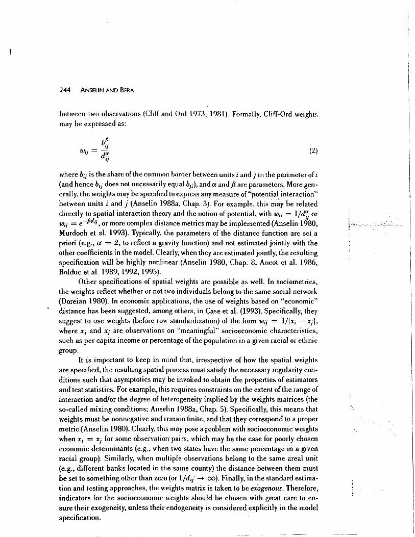
between two observations (Cliff and Onl I9n, 1981). Formally, Cliff-Ord weights may be expressed as:

b~ I)

w··-­''- da.

IJ

(2)

where b;j is the share of the common border bet ween units i and j in the perimeter of i (and hence b;j does not necessarily equal bji). and a and f3 are parameters. More gen­erally, the weights may be specified to express any measure of"potential interaction" between units i and j (Anselin 1988a, Chap. 3). For example, this ~~y be related directly to spatial interaction theory and the notion of potential, with Wij = 1/dij or w;j = e -Pdii, or more complex distance metrics may be implemented (Ansel in 1980, Murdoch et al. 1993). Typically, the parameters of the distance function are set a priori (e.g., a = 2, to reflect a gravity function) and not estimated jointly with the other coefficients in the model. Clearly, when they are estimated jointly, the resulting specification will be highly nonlinear (Anselin 1980, Chap. 8, Ancot et al. 1986, Bolduc et al. 1989, 1992, 1995).

Other specifications of spatial weights are possible as well. In sociometries, the weights reflect whether or not two individuals belong to the same social network (Doreian 1980). In economic applications, the use of weights based on "economic" distance has been suggested, among others, in Case et al. (1993). Specifically, they suggest to use weights (before row standardization) of the form Wij = 1/lx; - Xj I, wh~re Xi and Xj are observations on "meaningful" socioeconomic characteristics, such as per capita income or percentage of the population in a given racial or ethnic group.

It is important to keep in mind that, irrespective of how the spatial weights are specified, the resulting spatial process must satisfy the necessary regularity con­ditions such that asymptotics may be invoked to obtain the properties of estimators and test statistics. For example, this requires constraints on the extent of the range of interaction and/or the degree of heterogeneity implied by the weights matrices (the so-called mixing conditions~ Anselin 1988a, Chap. 5). Specifically, this means that weights must be nonnegative and remain finite, and that they correspond to a proper metric (Anselin 1980). Clearly, this may pose a problem with socioeconomic weights when xi = Xj for some observation· pairs, which may be the case for poorly chosen economic determinants (e.g., when two states have the same percentage in a given racial group). Similarly, when multiple observations belong to the same areal unit (e.g., different banks located in the same county) the distance between them must be set to s~mething other than zero (or 1/d;f-+ oo). Finally, in the standard estima­tion and testing approacht-.s, the weights matrix is taken to be exogerwus. Therefore, indicators for the socioeconomic weights should be chosen with great care to en­sure their exogeneity, unless their endogeneity is considered explicitly in the model specification.

;-" ... _,. __ , -.·---~~·...:..:...:.:

SPATIAL DEPENDENCE IN LINEAR REGRESSION MODElS 245

Operationally, the derivation of spatial weights from the location and spatial arrangement of observations must be carried out by means of a geographic informa­tion system, since for all but the smallest data sets a visual inspection of a map is im­practical (for implementation details, see Anselin et al. 1993a, 1993b, Anselin 1995, Can 1996). A mechanical construction of spatial weights, particularly when based on a distance criterion, may easily result in observations to become "unconnected" or isolated islands. Consequently, the row in the weights matrix that corresponds to these observations will consist of zero values. While not inherently invalidating es­timation or testing procedures, the unconnected observations imply a loss of degrees of freedom, since, for all practical purposes, they are eliminated from consideration in any "spatial" modeL This must be explicitly accounted for.

C. Spatial lag Operator

In time-series analysis, values for "neighboring" observations can be easily ex­pressed by means of a backward- or forward-shift operator on the one-dimensional time axis, yielding lagged variables Yz-k or Yt+k. where k is the desired shift (or lag). By contrast, there is no equivalent and unambiguous spatial shift operator. Only on a regular grid structure is there a potential solution, although not as straightforward as in the time domain. Following the so-called rook criterion for contiguity, each grid cell or vertex on a regular lattice, (i, j), has four neighbors: (i+ 1, j) (east), (i -1, j) (west), (i, j + 1) (north), and (i, j - 1) (south). Corresponding to this are four spa­

tially shifted variables: J'i+l.j· )'i-l,j· Yi.j+l• and Yi.j-1, each of which may require its own parameter in a spatial process modeL However, the rook criterion is not the only way spatial neighbors may be defined on a regular lattice, nor does the number of neighbors necessarily equal4. For example, following the queen criterion, each observation has eight neighbors, yielding eight spatially shifted variables; the four

for the rook criterion, as well as Jl-1.j+l, Ji"-l.j-1, Yi+l,j+1 and Yi+l.j-1· again each possibly with its own parameter. This notion of a spatial shift operator on a regular lattice has received only limited attention in the literature, mostly with a theoretical focus and primarily in statistical mechanics, in so-called Ising models (for details, see Cressie 1993, pp. 425-426).

On an irregular spatial structure, which characterizes most economic appli­cations, this formal notion of spatial shift is impractical, since the number of shifts would differ by observation, thereby making any statistical analysis extremely un­wieldy. Instead, the concept of a spatial lag operator is used, which consists of a weighted average of the values at neighboring locations. The weights are fixed and exogenous, similar to a distributed lag in time series. Formally, a spatial lag operator is obtained as the product of a spatial weights matrix W with the vector of observa­tions on a random variable y. or Wy. Each element of the resulting spatially lagged variable equals Lj Wij)J· i.e., a weighted average of they values in the neighbor set Si, since Wij = 0 for j fl. S;. Row standardization of the spatial weights matrix en-

246 ANSEUN AND BERA

sures that a spatial lag operation yields a smoothing of the neighboring values, since the positive weights sum to one.

Higher-order spatial lag operators are defined in a recursive manner, by ap­plying the spatial weights matrix to a lower-order lagged variable. For example, a

second-order spatial lag is obtained as W(Wy), or W2y. However, in contrast to time series, where such an operation is unambiguous, higher-order spatial operators yield redundant and circular neighbor relations, which must be eliminated to ensure proper estimation and inference (Biommestein 1985, Blommestein and Koper 1992, Anselin and Smirnov 1996).

In spatial econometrics, spatial autocorrelation is modeled by means of a func­tional relationship between a variable. y, or error term,£, and its associated spatial lag, respectively Wy for a spatially lagged dependent variable and WE for a spatially lagged error term. The resulting specifications are referred to as spatial lag and spa­tial error models, the general properties of which we consider next.

D. Spatial lag Dependence

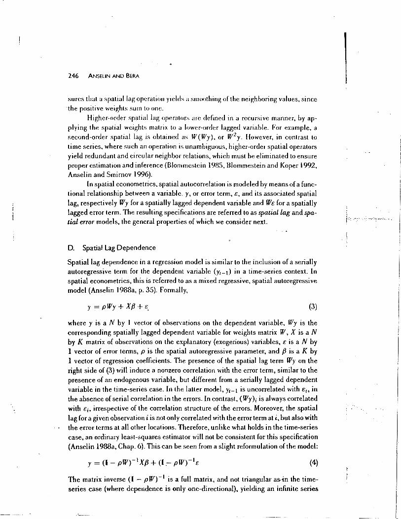
Spatial lag dependence in a regression model is similar to the inclusion of a serially autoregressive term for the dependent variable (y1 _ I) in a time-series context. In spatial econometrics, this is referred to as a mixed regressive, spatial autoregressive model (Anselin l988a, p. 35). Formally,

y = pWy + X{3 + £_ (3)

where y is a N by l vector of observations on the dependent variable, Wy is the

corresponding spatially lagged dependent variable for weights matrix W, X is a N by K matrix of observations on the explanatory (exogenous) variables, E is a N by 1 vector of error terms, p is the spatial autoregressive parameter, and {3 is a K by 1 vector of regression coefficients. The presence of the spatial lag term Wy on the right side of (3) will induce a nonzero correlation with the error term, similar to the presence of an endogenous variable, but different from a serially lagged dependent variable in the time-series case. In the latter model, Yt-l is uncorrelated with £, in the absence of serial correlation in the errors. In contrast, (W)'); is always correlated with £j, irrespective of the correlation structure of the errors. Moreover, the spatial

lag for a given observation i is not only correlated with the error term at i, but also with the error terms at all other locations. Therefore, unlike what holds in the time-series case, an ordinary least-squares estimator will not be consistent for this specification (Anselin 1988a, Chap. 6). This can be seen from a slight reformulation of the model:

y =(I- pW)- 1 Xf3 + (1.- pW)- 1£ (4)

The matrix inverse (I - pW)-1 is a full matrix, and not triangular as-in the time­series case (where dependence is only one-directional), yielding an infinite series

· ... :~ ... - .:~ -~~· :..:.. .:._. -~-~-

.. ,.

I

SPATIAL DEPENDENCE IN LINEAR REGRESSION MODELS 247

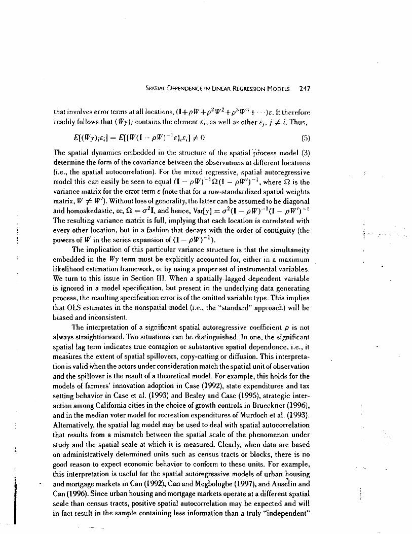
that involves error terms at all locations, (I+ p W + p 2 W2 + p:1 w:~ +- --)c. It therefore readily follows that (Wy)i contains the element E1 , as well as other Ej, j f i. Thus,

(S)

The spatial dynamics embedded in the structure of the spatial process model (3) determine the form of the covariance between the observations at different locations (i.e., the spatial autocorrelation). For the mixed regressive, spatial autoregressive model this can easily be seen to equal ((- pW)- 1 Q(l - pW')- 1, where Q is the variance matrix for the error term E {note that for a row-standardized spatial weights matrix, W =/= W'). Without loss of generality, the latter can be assumed to be diagonal and homoskedastic, or, Q = a-21, and hence, Var{y}= a 2(l- pW)- 1(1- pW')- 1

The resulting variance matrix is full, implying that each location is correlated with every other location, but in a fashion that decays with the order of contiguity (the powers of Win the series expansion of (l- pW)-1).

The implication of this particular variance structure is that the simultaneity embedded in the Wy term must be explicitly accounted for, either in a maximum likelihood estimation framework, or by using a proper set of instrumental variables. We turn to this issue in Section HI. When a spatially -lagged dependent variable is ignored in a model specifi<;ation, but present in the underlying data generating process, the resulting specification error is of the omitted variable type. This implies that OLS estimates in the nonspatial model (i.e., the "standard" approach) will be biased and inconsistent.

The interpretation of a significant spatial autoregressive coefficient p is not always straightfonvard. Two situations can be distinguished. In one, the significant spatial lag term indicates true contagion or substantive spatial dependence, i.e., it measures the extent of spatial spillovers. copy-catting or diffusion. This interpreta­tion is valid when the actors under consideration match the spatial unit of observation and the spillover is the result of a theoretical modeL For example, this holds for the models of farmers' innovation adoption in Case (1992}, state expenditures and tax setting behavior in Case et al. (1993} and Besley and Case (1995), strategic inter­action among California cities in the choice of growth controls in Brueckner (1996), and in the median voter model for recreation expenditures of Murdoch et al. {1993). Alternatively, the spatial lag model may be used to deal with spatial autocorrelation that results from a mismatch between the spatial scale of the phenomenon under study and the spatial scale at which it is measured. Clearly, when data are based on administratively determined units such as census tracts or blocks, there is no good reason to expect economic behavior to conform to these units. For example, this interpretation is useful for the spatial autoregressive models of urban ~ousing and mortgage markets in Can (1992). Can and Megbolugbe (1997), and Ansel in and Can ( 1996). Since urban housing and mortgage markets operate at a different spatial scale than census tracts. positive spatial autocorrelation may be expected and will in fact result in the sample containing less information than a truly "independent ..

;

i . ...

248 ANSELIN AND BERA

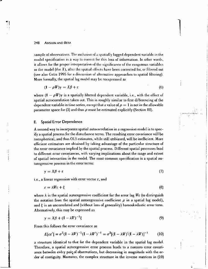
sample of observations. The inclusion of a spatially lagged dependent variable in the model specification is a way to correct for this loss of information. In other words, it allows for the proper inkrpretation of the significance of the exogenous variables in the model (the X), after the spatial effects have been corrected for, or filtered out (see also Getis 1995 for a discussion of alternative approaches to spatial filtering). More formally, the spatial lag model may be reexpressed as

(l- pW)y = X{J + c (6)

where (l - pW)y is a spatially filtered dependent variable, i.e., with the effect of spatial autocorrelation taken out. This is roughly similar to first differencing of the dependent variable in time series, except that a value of p = l is not in the allowable parameter space for (3) and thus p must be estimated explicitly (Section III).

E. Spatial Error Dependence

A second way to incorporate spatial autocorrelation in a regression model is to spec­ify a spatial process for the disturbance terms. The resulting error covariance will be nonspherical, and thus OLS estimates, while still unbiased, will be inefficiem. More efficient estimators are obtained by taking advantage of the particular structure of the error covariance implied by the spatial process. Different spatial processes lead to different error covariances, with varying implications about the range and extent of spatial interaction in the modeL The most common specification is a spatial au­toregressive process in the error terms:

y = X{J + c (7)

i.e., a linear regression with error vector c, and

c = A.Wt+~ (8)

where A. is the spatial autoregressive coefficient for the error lag We (to distinguish the notation from the spatial autoregressive coefficient p in a spatial lag model), and ~ is an uncorrelated and (without loss of generality) homoskedastic error term. Alternatively, this may be expressed as

y = X{J +(I- A.W)- 1 ~ (9)

From this follows the error covariance as

a structure identical to that for the dependent variable in the spatial lag model. Therefore, a spatial autoregressive error process leads to a nonzero error covari­ance between every pai~of observations, but decreasing in magnitude with the or­der of contiguity. Moreover. the complex structure in the inverse matrices in (lO)

l

--~.·- ~- -.- : . . --~ ::.::...· :.- ; ..

i

~

' ..

SPATIAL DEPENDENCE IN LINEAR REGRESSION MODELS 249

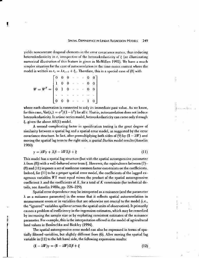
yields nonconstant diagonal elements in the error covariance matrix, thus inducing

heteroskedasticity in c, irrespective of the hetcroskedasticity of~ (an illuminating numerical illustration of this feature is given in McMillen 1992). We have a much

simpler situation for the case of autocorrelation in the time-series context where the ' model is written as €t = Act-1 + ~ t. Therefore, this is a special case of (8) with

0 0

1 0

W=WT= 0 1

0 0

0

0

0

0

0 0

0 0

0 0

1 0

where each observation is connected to only its immediate past value. As we know, for this case, Var(e,) = a 2 /(1- A 2) for all t. That is, autocorrelation does not induce heteroskedasticity. In a time-series model, heteroskedasticity can come only through

~'given the above AR(l) model. A second complicating factor in specification testing is the great degree of

similarity between a spatial lag and a spatial error model, as suggested by the error covariance structure. In fact, after premultiplying both sides of (9) by (I - A.W) and moving the spatial lag term to the right side, a spatial Durbin model results (Anselin

1980):

y = A.Wy + X{3 - AWX{3 + ~ (11)

This model has a spatial lag structure (but with the spatial autoregressive parameter A from (8)) with a well-behaved error term~. However, the equivalence between (7)­(8) and (ll) imposes a set of nonlinear common factor constraints on the coefficients.

Indeed, for (II) to be a proper spatial error model, the coefficients of the lagged ex­

ogenous variables WX must equal minus the product of the spatial autoregressive coefficient A and the coefficients of X, for a total of K constraints (for technical de­

tails, see Anselin I988a, pp. 226-229). Spatial error dependence may be interpreted as a nuisance (and the parameter

A as a nuisance parameter) in the sense that it reflects spatial autocorrelation in measurement errors or in variables that are otherwise not cruci~l to the model (i.e.,

the "ignored" variables spillover across the spatial units of observation). It primarily causes a problem of inefficiency in the regression estimates, which may be remedied by increasing the sample size or by exploiting consistent estimates of the nuisance

parameter. For example, this is the interpretation offered in the model of agricultural land values in Benirschka and Binkley (I994).

The spatial autoregressive error model can also be expressed in terms of spa­tially filtered variables, but slightly different from (6). After moving the spatial lag variable in (II} to the left hand side, the following expression results:

(I - AW)y = (I - A.W)X,B + ~ (12}

•· \.

' j !' I

II t.

L 1:

250 ANSELIN AND BERA

This is a regression model with spatially filtered dependent and explanatory vari­

ables and with an uncorrelated error term ~, similar to first differencing of both y and X in time-series models. As in the spatial lag model,)... = l is outside the pa­

rameter space and thus A must be estimated jointly with the other coefficients of the

model (see Section Ill). Several alternatives to the spatial autoregressive error process (8) have been

suggested in the literature, though none of them have been implemented much in practice. A spatial moving average error process is specified as (Cliff and Ord l98l,

Haining l988, l990):

t: = yW~ + ~ (13)

where y is the spatial moving average coefficient and~ is an uncorrelated error term. This process thus specifies the error term at each location to consist of a location­

specific part, ~i ("innovation"}, as well as a weighted average (smoothing} of the

errors at neighboring locations, W~. The resulting error covariance matrix is

£[a']= a-2(l + yW)(l + yW') = o-2[l + y(W + W') + y 2WW'] (14)

Note that in contrast to (lO), the structure in (l4) does not yield a full covariance ma­

trix. Nonzero covariances are only found for first-order ( W + W') and second-order ( WW') neighbors, thus implying much less overall interac-tion than the autoregres­

sive process. Again, unless all observations have the same number of neighbors and

identical weights, the diagonal elements of (l4) will not be constant, inducing het­

eroskedasticity in£, irrespective of the nature of~-A very similar structure to (l3) is the spatial error components model of Kele-

jian and Robinson (l993, 1995), in which the disturbance is a sum of two indepen­dent error terms, one associated with the "region" (a smoothing of neighboring errors)

and one which is location-specific:

£ = w~ +1ft (15)

with ~ and 1ft as independent error components. The resulting error covariance is

(16)

where a-~ and a-: are the variance components associated with respectively the

location-specific and regional error parts. The spatial interaction implied by (16)

is even more limited than for (14). pertaining only to the first- and second-order

neighbors contained in the nonzero elements of WW'. Heteroskedasticity is implied

unless all locations have the same number of neighbors and identical weights, a sit­

uation excluded by the assumptions needed for the proper asymptotics in the model

(Kelejian and Robinson 1993, p. 301). In sum, every type of spatially dependent error process induces heteroskedas-

ticity as well as spatially autocorrelated errors, which will greatly complicate spec­

ification testing in practice. Note that the "direct representation" approach based

... ·-:. .. ·'

I I

SPATIAL DEPENDENCE IN LiNEAR REGRESSION MODELS 25 I

on geostatistical principles docs not suffer from this problem. For example, in Du­bin (1988, 1992), the elements of the error covariance matrix are expressed di­rectly as functions of the distance d,

1 between the corresponding observations, e.g.,

E[EiEj] = yle(-d,,!Y2 >, with Yt and Y2 as parameters. Since e-di.IY2 = 1, irrespec­

tive of the value of y2, the errors E will be homoskedastic unless explicitly modeled

otherwise.

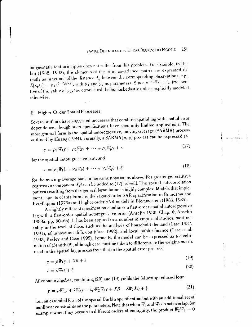
F. Higher-Order Spatial Processes

Several authors have suggested processes that combine spatial lag with spatial error dependence, though such specifications have seen only limited applications. The most general form is the spatial autoregressive, moving-average (SARMA) process outlined by Huang (1984). Formally, a SARMA(p, q) process can be expressed as

(17)

for the spatial autoregressive part, and

(18)

for the moving-average part, in the same notation as above. For greater generality, a regressive component X{3 can be added to (17) as well. The spatial autocorrelation pattern resulting from this general formulation is highly complex. Models that imple­ment aspects of this form are the second-order SAR specification in Brandsma and Ketellapper (1979a) and higher-order SAR models in Blommestein (1983, 1985).

A slightly different specification _combines a first-order spatial autoregressive

lag with a first-order spatial autoregressive error (Anselin 1980, Chap. 6; Anselin 1988a, pp. 60-65). It has been applied in a number of empirical studies, most no­tably in the work of Case, such as the analysis of household demand (Case 1987, 1991), of innovation diffusion (Case 1992), and local public finance (Case et al. 1993, Besley and Case 1995). F0rmally, the model can be expressed as a combi­nation of (3) with (8), although care must be taken to differentiate the weights matrix

used in the spatial lag process from that in the spatial error process:

y = p Wt y + X {3 + c

E = .AW2E + ~ After some algebra, combining (20) and (19) yields the following reduced form:

(19)

(20)

(21)

i.e., an extended form of the spatial Durbin specification but with an additional set of nonlinear constraints on the parameters. Note that when W1 and W2 do not overlap, for example when they pertain to different orders of contiguity, the product W2 Wt = 0

~~·-.. :.. :.

- -~--

252 ANSELIN AND BERA

and (21) reduces to a biparametric spatial lag formulation, albeit with additional

constraints on the parameters. On the other hand, when W1 and W2 are the same, the parameters pandA arc only identified when at least one exogenous variable is

included in X (in addition to the constant term) and when the nonlinear constraints

are enforced (Ansel in 1980, p. 176). When WI = w2 = w' the model becomes

y = (p + A)Wy- ApW2y + X{3- AWX{3 + ~ (22)

Clearly, the coefficients of Wy and W2y alone do not allow for a separate identi­

fication of p and A. Using the nonlinear constraints between the f3 and -A{3 (the

coefficients of X and WX) yields an estimate of A, but this will only be unique when

the constraints are strictly enforced. Similarly, an estimate of A may result in two

possible estimates for p (one using the coefficient of Wy, the other of W2 y) unless

the nonlinear constraints are strictly enforced. This considerably complicates esti­mation strategies for this modeL In contrast, a SARMA(l, 1) model does not suffer

from this problem. In empirical practice, an alternative perspective on the need for higher-order

processes is to consider them to be a result of a poorly specified weights matrix rather

than as a realistic data generating process. For example, if the weights matrix in a spatial lag model underbounds the true spatial interaction in the data, there will be

remaining spatial error autocorrelation. This may lead one to implement a higher­

order process, while for a properly specified weights matrix no such process is needed (see Florax and Rey 1995 for a discussion of the effects of misspecified weights). In

practice, this will require a careful specification search for the proper form of the

spatial dependence in the model, an issue to which we return in Section IV First, we

consider the estimation of regression models that incorporate spatial autocorrelation

of a spatial lag or error form.

Ill. ESTIMATING SPATIAL PROCESS MODELS

Similar to when serial dependence is present in the time domain, classical sam­

pling theory no longer holds for spatially autocorrelated data, and estimation and

inference must rely on the asymptotic properties of stochastic processes. In essence,

rather than considering N observations as independent pieces of information, they

are conceptualized as a single realization of a process. In order to carry out mean­

ingful inference on the parameters of such a process, constraints must be imposed

on both heterogeneity and the range of interaction. While many properties of esti­

mators for spatial process models may be based on the same principles as developed

for dependent (and heterogeneous) processes in the time domain (e.g., the formal

properties outlined in White 1984, 1994), there are some important differences as

welL Before covering specific estimation procedures, we discuss these differences

in some detail, focusing in particular on the notion of stationarity in space and the

SPATIAL DEPENDENCE IN LINEAR REGRESSION MODELS 253

distinction between simultaneous and conditional spatial processes. Next, we turn to a review of maximum likelihood and instrumental variables estimators for spat1al regression models. We close with a brief discussion of operational implementation arid software issues.

A Spatial Stochastic Processes

As in the time domain, in order to carry out meaningful inference for a spatial pro­cess, some degree of equilibrium must be assumed in the sense that the stochastic generating mechanism is taken to work uniformly over space. In a strict sense, a notion of "spatial stationarity" accomplishes this objective since it imposes the con­dition that any joint distribution of the random variable under consideration over a subset of the locations depends only on the relative position of these observations in terms of their relative orientation {angle) and distance. Even stricter is a notion of isotropy, for which only distance matters and orientation is irrelevant. For practical purposes, the notions of stationarity and isotropy are too demanding and not veri­fiable. Hence, weaker conditions are typically imposed in the form of stationarity of the first (mean) and second moments (variance, covariance, or spatial autocor­relation). Even weaker requirements follow from the so-called intrinsic hypothesis in geostatistics, which requires only stationarity of the variance of the increments, leading to the notion of a variogram (for technical details, see Ripley 1988, pp. 6-7; Cressie 1993, pp. 52-68).

For stationary processes in the time domain, the careful inspection of auto­covariance and autocorrelation functions is a powerful aid in the identification of the model, e.g., following the familiar Box-Jenkins approach (Box et al. 1994). One could transpose this notion to spatial processes and consider spatial autocorrela­tion functions indexed by order of contiguity as the basis for model identification. However, as Hooper and Hewings {1981) have shown, this is only appropriate for a very restrictive class of spatial processes on regular lattice structures. For applied work in empirical economics, such restrictions are impractical and the spatial de­pendence in the model must be specified explicitly by means of the spatial lag and spatial error structures reviewed in the previous section. Inference may be based on the asymptotic properties (central limit theorems and laws of large numbers) of so-called dependent and heterogeneous processes, as developed in White and Oo­mowitz (1984) and White (1984, 1994). Central to these notions is the concept of mixing sequences, allowing for a trade-off between the range of dependence and the extent of heterogeneity (see Anselin l988a, pp. 45-46 for an intuitive extension of this to spatial econometric models). While rigorous proofs of these properties have not been derived for the explicit spatial case, the notion of a spatial weights matrix based on a proper metric is general enough to meet the criteria imposed by mixing conditions. In a spatial econometric approach then, a spatial lag model is considered to be a special case of simultaneity or endogeneity with dependence, and a spatial

254 ANSELIN AND BERA

error model is a special case of a nonspherical error term, both of which can be

tackled by means of generally established econometric theory, though not as direct extensions of the time-series analog.

The emphasis on "simultaneity" in spatial econometrics differs somewhat from

the approach taken in spatial statistics, where conditional models are often consid­

ered to be more natural (Cressie 1993, p. 410). Again, the spatial case differs sub­stantially from the time,-series one since in space a conditional and simultaneous

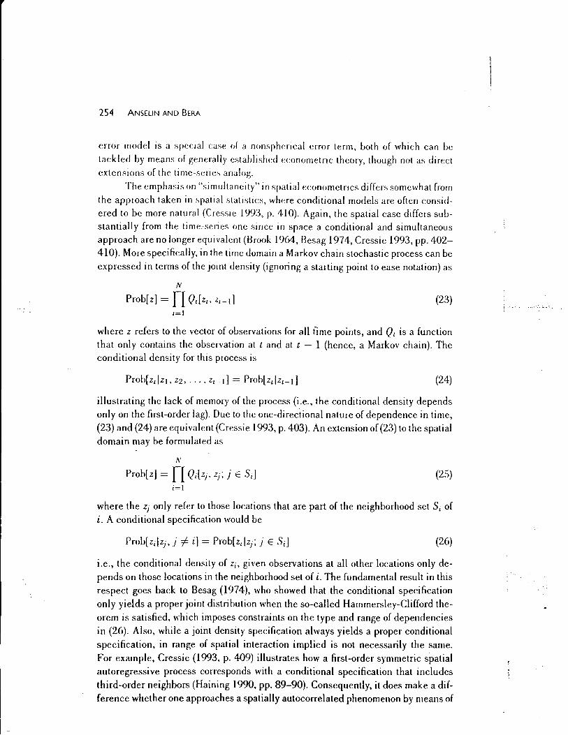
approach are no longer equivalent (Brook 1964, Besag 1974, Cressie 1993, pp. 402-410). More specifically, in the time domain a Markov chain stochastic process can be

expressed in terms of the joint density (ignoring a starting point to ease notation) as

N

Prob[z] = n Ot[zl> Zt-d (23) t=l

where z refers to the vector of observations for all time points, and Q1 is a function that only contains the observation at t and at t - I (hence, a Markov chain). The conditional density for this process is

(24)

illustrating the lack of memory of the process (i.e., the conditional density depends only on the first-order lag). Due to the one-directional nature of dependence in time,

(23) and (24) are equivalent (Cressie 1993, p. 403). An extension of (23) to the spatial domain may be formulated as

"' Prob[z] = n Qi[z,. Zj; j E Si] (25) i=l

where the ZJ only refer to those locations that are part of the neighborhood set Si of

i. A conditional specification would be

(26)

i.e., the conditional density of Zj, given observations at all other locations only de­

pends on those locations in the neighborhood set of i. The fundamental result in this

respect goes back to Besag (1974), who showed that the conditional specification

only yields a proper joint distribution when the so-called Hammersley-Clifford the­

orem is satisfied, which imposes constraints on the type and range of dependencies

in (26). Also, while a joint density specification always yields a proper conditional

specification, in range of spatial interaction implied is not necessarily the same.

For example, Cressie (1993, p. 409) illustrates how a first-order symmetric spatial

autoregressive process corresponds with a conditional specification that includes

third-order neighbors (Haining 1990, pp. 89-90). Consequently, it does make a dif­

ference whether one approaches a spatially autocorrelated phenomenon by means of

I -

SPATIAL DEPENDENCE IN LINEAR REGRESSION MODELS 255

(26) versus (25). This also has implications for the substantive interpretation of the model results, as illustrated for an analysis of retail pricing of gasolme in Haining

(1984). [n practice, it is often easier to estimate a conditional model, especially for

nonnormal distributions (e.g., auto-Poisson, autologistic). Also, a conditional speci­fication is more appropriate when the focus is on spatial prediction or interpolation. For general estimation and inference, however, the constraints imposed on the type and range of spatial interaction in order for the conditional density to be proper are often highly impractical in empirical work. For example, an auto-Poisson model (conditional model for spatially autocorrelated counts) only allows negative autocor­relation and hence is inappropriate for any analysis of clustering in space.

In the remainder, our focus will be exclusively on simultaneously specified models, which is a more natural approach from a spatial econometric perspective

(Anselin 1988a, Cressie 1993, p. 410).

B. Maximum Likelihood Estimation

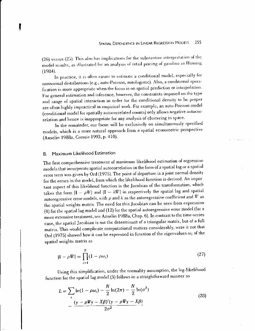
The first comprehensive treatment of maximum likelihood estimation of regression models that incorporate spatial autocorrelation in the form of a spatial lag or a spatial error term was given by Ord (1975). The point of departure is a joint normal density for the errors in the model, from which the likelihood function is derived. An impor­tant aspect of this likelihood function is the Jacobian of the transformation, which takes the form II - pWI and II - AWl in respectively the spatial lag and spatial autoregressive error models, with pandA as the autoregressive coefficient and Was the spatial weights matrix. The need for this Jacobian can be seen from expression (4) for the spatial lag model and (12) for the spatial autoregressive error model (for a more extensive treatment, see Anselin 1988a, Chap. 6). In contrast to the time-series case, the spatial Jacobian is not the determinant of a triangular matrix, but of a full matrix. This would complicate computational matters considerably, were it not that Ord (1975) showed how it can be expressed in function of the eigenvalues Wi of the

spatial weights matrix as

N

II- pWI =no- PWi) (27)

i=l

Using this simplification, under the normality assumption, the log-likelihood

function for the spatial lag model (3) follows in a straightforward manner as

" N N 2 L = ~ ln(l - pwi) - 2ln(2rr)- 2 ln(a )

I

(y- pWy- X{J)'(y- pWy- X{J)

2a2

(28)

'; .. '. i 1

256 ANSELIN AND BERA

in the same notation as used in Section II. This expression clearly illustrates why,

in contrast to the time-series case, ordinary least squares (i.e., the minimization of the last term in (28)) is not maximum likelihood, since it ignores the Jacobian term.

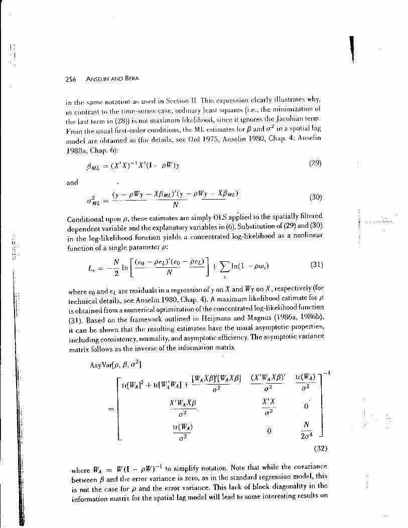
From the usual first-order conditions, th<: ML estimates for f3 and o-2 in a spatial lag

model are obtained as (for details, see Ord 1975, Anselin 1980, Chap. 4: Anselin

l988a, Chap. 6):

and

f3ML = (X'X)- 1X'(I- pW)y (29)

2 0" ML =

(y- pWy- Xf3Md'(y- pWy- Xf3MJJ

N (30)

Conditional upon p, these estimates are simply OLS applied to the spatially filtered dependent variable and the explanatory variables in (6). Substitution of {29) and (30)

in the log-likelihood function yields a concentrated log-likelihood as a nonlinear

function of a single parameter p:

Lc = -: ln [(eo- peL); eo -peL)]+ L ln(l - pw;)

'

(31)

where eo and eL are residuals in a regression of yon X and Wy on X, respectively (for

technical details, see Anselin 1980, Chap. 4). A maximum likelihood estimate for p is obtained from a numerical optimization of the concentrated log-likelihood function

(31). Based on the framework outlined in Heijmans and Magnus (1986a, l986b), it can be shown that the resulting estimates have the usual asymptotic properties, including consistency, normality, and asymptotic efficiency. The asymptotic variance

matrix follows as the inverse of the information matrix

AsyVar[p, {3, o-2]

tr(WA]2 + tr(W~WA] + [WAXJ3]';WAXJ3] . (J"

X' X a-2

0

-I

0

(32)

where WA = W(l - pW)- 1 to simplify notation. Note that while the covariance

between f3 and the error variance is zero, as in the standard regression model, this

is not the case for p and the error variance. This lack of block diagonality in the

information matrix for the spatial lag model will lead to some interesting results on

,,--:..:._:

J SPATIAL DEPENDENCE IN UNEAR REGRESSION MODELS 257

the structure of specification tests, to which we turn in Section IV It is yet another distinguishing characteristic between the spatial case and its analog in time series.

Maximum likelihood estimation of the models with spatial error autocorrela­tion that were covered in Section ILE can be approached by considering them as special cases of general parametrized nonspherical error terms, for which E[t:t:'J = a-2 Q(8), withe as a vector of parameters. For example, from (32) for a spatial au­

toregressive error term, it follows that

Q(A) =[(I- AW)'(I- AW) r 1 (33)

As shown in Anselin (1980, Chap. 5), maximum likelihood estimation of such spec­ifications can be carried out as an application of the general framework outlined in Magnus (1978). Most spatial processes satisfy the necessary regularity conditions, although this is not necessarily the case for direct representation models (Mardia and Marshalll984, Warnes and Ripley 1987, Mardia and Watkins 1989). Under the assumption of normality, the log-likelihood function takes on the usual form:

1 N N 2 L =--In lf2 (A )I - - ln(2rr) - - ln(o- ) 2 2 2

(y- Xt3)'S1(A)- 1(y- X{J)

2a2

(34)

for example, with Q (A) as in (33). First-order conditions yield the familiar general­

-ized least-squares estimates for {3, conditional upon A:

(35)

For a spatial autoregressive error process, Sl(A)-1 = (I- AW)'(I- AW), so that for known A, the maximum likelihood estimates are equivalent toOLS applied to the spatially filtered variables in (12). Note that for other forms of error dependence, the GI.S expression {35) will involve the inverse of an N by N error covariance matrix. For example, for the spatial moving average errors, as in (13), Q (y)- 1 = [I +y(W + W') + y 2 WW']- 1, which does not yield a direct expression in terms of spatially

transformed y and X. Obtaining a consistent estimate for A is not as straightforward as in the time­

series case. As pointed out, OLS does not yield a consistent estimate in a spatial lag modeL It therefore cannot be used to obtain an estimate for A from a regression of residuals eon We, as in the familiar Cochrane-Orcutt procedure for serially autore­gressive errors in the time domain. Instead, an explicit optimization of the likelihood function must be carried out. One approach is to use the iterative solution of the first­

order conditions in Magnus {1978, p. 283):

[(aQ- 1

) ] , (aQ- 1) tr -- Q =e -- e

dA oA (36)

258 ANSELIN AND 8ERA

where e = y - X{J are CLS residuals. For a spatial autoregressive error process,

an- 1 /JA = - W - W' + ).W' W. Solution of condition (36) can be obtained by

numerical means. Alternatively, the GLS expression for fJ and similar solution of

the first-order conditions for a 2 can be substituted into the log-likelihood function

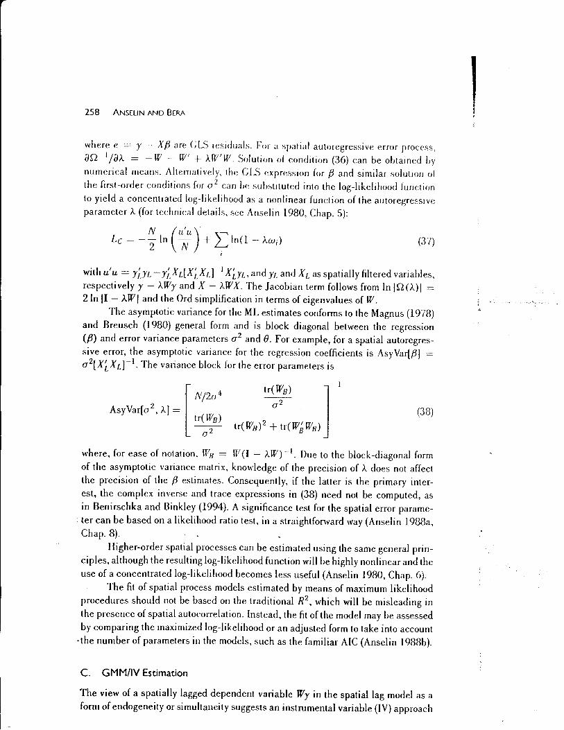
to yield a concentrated log-likelihood as a nonlinear function of the autoregressive parameter A (for technical details, see Anselin 1980, Chap. S):

N (u'u)· ~ Lc = - 2 ln N + L ln(l- Aw;) (37) l

with u'u = rfn -r;_ XL[ X;_ XL]- 1 X~n, and YL and XL as spatially filtered variables, respectively y- AWy and X- AWX. The Jacobian term follows from In jQ(A)I = 2ln II -.AWl and the Ord simplification in terms of eigenvalues of W.

The asymptotic variance for the ML estimates conforms to the Magnus (1978)

and Breusch (1980) general form and is block diagonal between the regression

(fJ) and error variance parameters a 2 and 8. For example, for a spatial autoregres­sive error, the asymptotic variance for the regression coefficients is AsyVar[{J] a2[X~XL]- 1 . The variance block for the error parameters is

(38)

where, for ease of notation, Ws = W (I - AW) -I. Due to the block -diagonal form

of the asymptotic variance matrix, knowledge of the precision of A does not affect

the precision of the fJ estimates. Consequently, if the latter is the primary inter­

est, the complex inverse and trace expressions in (38) need not be computed, as

in Benirschka and Binkley (1994). A significance test for the spatial error parame­

ter can be based on a likelihood ratio test, in a straightforward way (Anselin 1988a, Chap. 8).

Higher-order spatial processes can be estimated using the same general prin­ciples, although the resulting log-likelihood function will be highly nonlinear and the

use of a concentrated log-likelihood becomes less useful (Anselin 1980, Chap. 6).

The fit of spatial process models estimated by means of maximum likelihood

procedures should not be based on the traditional R2, which will be misleading in

the presence of spatial autocorrelation. Instead, the fit of the model may be assessed

by comparing the maximized log-likelihood or an adjusted form to take into account

·the number of parameters in the models, such as the familiar AIC (Anselin 1988b).

C. GMM/IV Estimation

The view of a spatially lagged dependent variable Wy in the spatial lag model as a

form of endogeneity or simultaneity suggests an instrumental variable (IV) approach

r SPATIAL DEPENDENCE IN LINEAR REGRESSION MODELS 259

to estimation (Anselin 1980, l988a, Chap. 7; l990b). Since the main problem is the correlation between Wyand the (:rror term in (3), the choice of proper instruments for Wy will yield consistent estimates. However, as usual, the efficiency of these estimates depends crucially on the choice of the instruments and may be poor in small samples. On the other hand, in contrast to the maximum likelihood approach just outlined, IV estimation does not require an assumption of normality.

Using the standard econometric results (for a review, see Bowden and Turk­ington 1984), and with Q asaP by N matrix (P ~ K + l) of instruments (including K "exogenous" variables from X), the IV or 2SLS estimate follows as

/hv = [Z'Q(Q'Q)- 1Q'zr' z'Q(Q'Q)- 1Q'r (39)

with Z = [Wy X], AsyVar(fhv) = a 2[Z'Q(Q'Q)- 1Q'Zr 1, and a 2 = (y- Zf31v)'

(y- Zf3,v)/N. Clearly, this approach can also be applied to models where other endogenous

variables appear in addition to the spatially lagged dependent variable, as in a si­multaneous equation context, provided that the instrument set is augmented to deal with this additional endogeneity. It also forms the basis for a bootstrap approach to the estimation of spatial lag models (Anselin l990b). Moreover, it is easily extended to deal with more complex error structures, e.g., reflecting forms of heteroskedastic­ity or spatial error dependence (Anselin l988a, pp. 86-88). The formal properties of such an approach are derived in Kelejian and Robinson (1993) for a general methods of moments estimator (GMM) in the model y = p Wy + X{3 + E with spatial error

components, E = w~ + 1/J. The GMM estimator takes the form

(40)

where Q is a consistent estimate for the error covariance matrix. The asymptotic vari­ance for f3cMM is [Z'Q(Q'QQ)- 1Q'Zr 1. For the spatial error components model, Kelejian and Robinson (1993, pp. 302-304) suggest an estimate for Q = ~~I + ~2 WW', with ~~ and ~2 as the least-squares estimates in an auxilliary regression of the squared IV residuals (y - Zf31d on a constant and the diagonal elements

ofWW'. A particularly attractive application of GLS-IV estimation in s~atiallag mod-

els is a special case of the familiar White heteroskedasticity-consistent covariance estimator (White 1984, Bowden and Turkington 1984, p. 91). The estimator is as in (40), but Q'QQ is estimated by Q'QQ, where Q is a diagonal matrix of squared IV residuals, in the usual fashion. This provides a way to obtain consistent estimates for the spatial autoregressive l)arameter p in the presence of heteroskedasticity of

unknown form, often a needed feature in applied empirical work. A crucial issue in instrumental variables estimation is the choice of the instru­

ments. In spatial econometrics, several suggestions have been made to guide these­lection of instruments for Wy (for a review, see Anselin l988a, pp. 84-86~ Land and Deane 1992). Recently, Kelejian and Robinson (1993 p. 302) formally demonstrated

260 ANSELIN AND BERA

the consistency of fJcMM in the spatial lag model with instruments consisting of first­

order and higher-order spatially lagged explanatory variables (WX, W2 X, etc.).

An important feature of the instrumental variables approach is that estima­

tion can easily be carried out by rneans of standard econometric software, provided

that the spatial lags can be computed as the result of common matrix manipulations

(Anselin and Hudak 1992). In contrast, the maximum likelihood approach requires

specialized routines to implement the nonlinear optimization of the log-likelihood

(or concentrated log-likelihood). We next tum to some operational issues related to this.

D. Operational Implementation and Illustration

To date, none of the widely available econometric software packages contain specific

routines to implement maximum likelihood estimation of spatial process models or to carry out specification tests for spatial autocorrelation in regression models. This lack of attention to the analysis of the lattice data structures that are most relevant

in empirical economics contrasts with a relatively large range of software for spatial

data analysis in the physical sciences, geared to point patterns and geostatistical

data. Examples of these are the GSLIB library (Deutsch and Journel 1992) and the

recent S+Spatialstats add-on to the S-PLUS statistical software (MathSoft 1996). While the latter does include some analyses for lattice data, estimation is limited to

maximum likelihood of spatial error models with autoregressive or moving-average

structures. However, the spatial lag model is not covered and specification diagnos­

tics are totally absent.

The only self-contained software package specifically geared to spatial econo­

metric analysis in SpaceStat (Anselin 1992b, 1995). It contains both maximum like­

lihood and instrumental variables estimators for spatial lag and error models, as well

as ways to estimate heteroskedastic specifications and a wide range of diagnostics

for spatial effects. In addition, SpaceStat also includes extensive features to carry out

exploratory spatial data analysis as well as utilities to create and manipulate spatial

weights matrices and interface with geographic information systems.

There are two major practical issues that must be resolved to implement the

estimation of spatial lag and spatial error models. The first is the need to construct

spatially lagged variables from observations on the dependent variable or residual

term. This is relevant for both instrumental variables (IV, 2SLS, GMM) as well as

maximum likelihood estimation. In principle, the lag can be computed as a simple

matrix multiplication of the spatial weights matrix W with the vector of observa­

tions, say Wy. This is straightforward to implement in most econometric software

packages that contain matrix algebra routines (specific examples for Gauss, Splus,

Limdep, Rats and Shazam are given in Anselin and Hudak 1992, Table 2, p. 514).

In practice, however, the size of the matrix that can be manipulated by economet­

ric software is severely limited and insufficient for most empirical applications, un-

SPATIAL DEPENDENCE IN LINEAR REGRESSION MODELS 261

less sparse matrix routines can be exploited (avoiding the need to store a full N by

- N matrix). This is increasingly the case in state-of-the-art matrix algebra packages

(e.g., Matlab, Gauss), but still fairly uncommon in application-oriented economet­

ric software; hence, the computatiOn of spatial lags will typically necessitate some

programming effort on the part of the user (the construction of spatial lags based on sparse spatial weights formats in SpaceStat is discussed in Anselin 1995). Once the

spatial lagged dependent variables are computed, IV estimation of the spatial lag

model can be carried out with any standard econometric package.

The other major operational issue pertains only to maximum likelihood esti­

mation. It is the need to manipulate large matrices of dimension equal to the number

of observations in the asymptotic variance matrices (32) and (38) and in the Jaco­

bian term (27) of the log-likelihoods {31) and (3 7). In contrast to the time-series case,

the matrix W is not triangular and hence a host of computational simplifications are not applicable. The problem is most serious in the computation of the asymptotic

variance matrix of the maximum likelihood estimates. The inverse matrices in both WA = W(l- pW)- 1 of{32) and WB = W(l- .AW)- 1 of(38) are full matrices which

do not lend themselves to the application of sparse matrix algorithms. For low values

of the autoregressive parameters, a power expansion of (I- pW)- 1 or (1- .AW)- 1

may be a reasonable approximation to the inverse, e.g., (I- pW)- 1 = Lk pkWk+

error, with k = 0, 1, ... , K, such that pK < 8, where 8 is a sufficiently small value.

However, this will involve some computing effort in the construction of the powers of

the weights matrices and is increasingly burdensome for higher values of the autore­

gressive parameter. In general, for all practical purposes, the size of the problem for

which an asymptotic variance matrix can be computed is constrained by the largest matrix inverse that can be carried out with acceptable numerical precision in a given

software/hardware environment. Jn current desktop settings, this typically ranges from a few h1mdred to a few thousand observations. While this makes it impossible

to compute asymptotic t-tests for all the parameters in spatial models with very large

numbers of observations, it does not preclude asymptotic inference. In fact, as we ar­

gued in Section III.B, due to the block diagonality of the asymptotic variance matrix

in the spatial error case, asymptotic t-statistics can be constructed for the estimated

{3 coefficients without knowledge of the precision of the autoregressive parameter A (see also Benirschka and Binkley 1994, Pace and Barry 1996). Inference on the au­

toregressive parameter can be based on a likelihood ratio test (Anselin 1988a, Chap.

6). A similar approach can be taken in the spatial lag modeL However, in contrast

to the error case, asymptotic t-tests can no longer be constructed for the estimated f3 coefficients, since the asymptotic variance matrix (32) is not block diagonaL Instead,

likelihood ratio tests must be considered explicitly for any subset of coefficients of

interest (requiring a separate optimization for each specification; see Pace and Barry

1997).

With the primary objective of obtaining consistent estimates for the parameters

in spatial regression models, a number of authors have suggested ways to manipu-

262 ANSELIN AND BERA

late popular statistical and econometric software packages in order to maximize the log-likelihoods (28) and (37). Examples of such efforts are routines for ML estima­tion of the spatial lag and spatial autoregressive error model in Systat, SAS, Gauss, Limdep, Shazam, Rats and S-PLUS (Bivand 1992, Griffith 1993, Anselin and Hu­dak I992, Anselin et al. 199.'3b). The common theme among these approaches is to find a way to convert the log-likelihoods for the spatial models to a form amenable for use with standard nonlinear optimization routines. Such routines proceed incre­mentally, in the sense that the likelihood is built up from a sum of elements that correspond to individual observations. At first sight, the Jacobian term in the spatial models would preclude this. However, taking advantage of the Ord decomposition in terms of eigenvalues, pseudo-observations can he constructed for the elements of the Jacobian. Specifically, each term I - pw; is considered to correspond to a pseudo­variable Wi, and is summed over all "observations." For example, for the spatial lag model, the log-likelihood (ignoring constant terms) can be expressed as

L = L [In(! - pw;)- In~') - (y;- p(~~;;- x;,B)'] L

(41)

which fits the format expected by most nonlinear optimization routines. Examples of practical implementations are listed in Anselin and Hudak (1992, Table 10, p. 533) and extensive source code for various econometric software packages is given in Ansel in et al. (1993h ).

One pro!:>lem with this approach is that the asymptotic variance matrices com­puted by the routines tend to he based on a numerical approximation and do not necessarily correspond to the analy·tical expressions in (32) and (38). This may lead to slight differences in inference depending on the software package that is used {Ansel in and Hudak I992, Table I 0, p. 533). An alternative approach that does not require the computation of eigenYalues is based on sparse matrix algorithms to effi­ciently compute the determinant of the Jacobian at each iteration of the optimization routine. While this allows the estimation of models for very large data sets (tens of thousands of observations), for example, by using the specialized routines in the Mat­lab software, this does not solve the asymptotic variance matrix problem. Inference therefore must be based on likelihood ratio statistics (for details and implementation, see Pace and Barry 1996, 1997).

To illustrate the various spatial models and their estimation, the results for the parameters in a simple spatial model of crime estimated for 49 neighborhoods in Columbus, Ohio, are presented in Table I. The model and results are based on Anselin (l988a, pp. 187-196) and have been used in a number of papers to bench­mark different estimators and specification tests (e.g., McMillen 1992, Getis 1995,

Anselin et al. 1996, LeSage 1997). The data are also available for downloading via the internet from http://www.rri. \n'u.edu/spacestat.htm. The estimates reported in Table 1 include OLS in the standard regression model, OLS (inconsistent), ML, IV, and.heteroskedastic-robust IV for the spatial lag model, and ML for the spatial error

r SPATIAL DEPENDENCE IN LINEAR REGRESSION MODELS 263

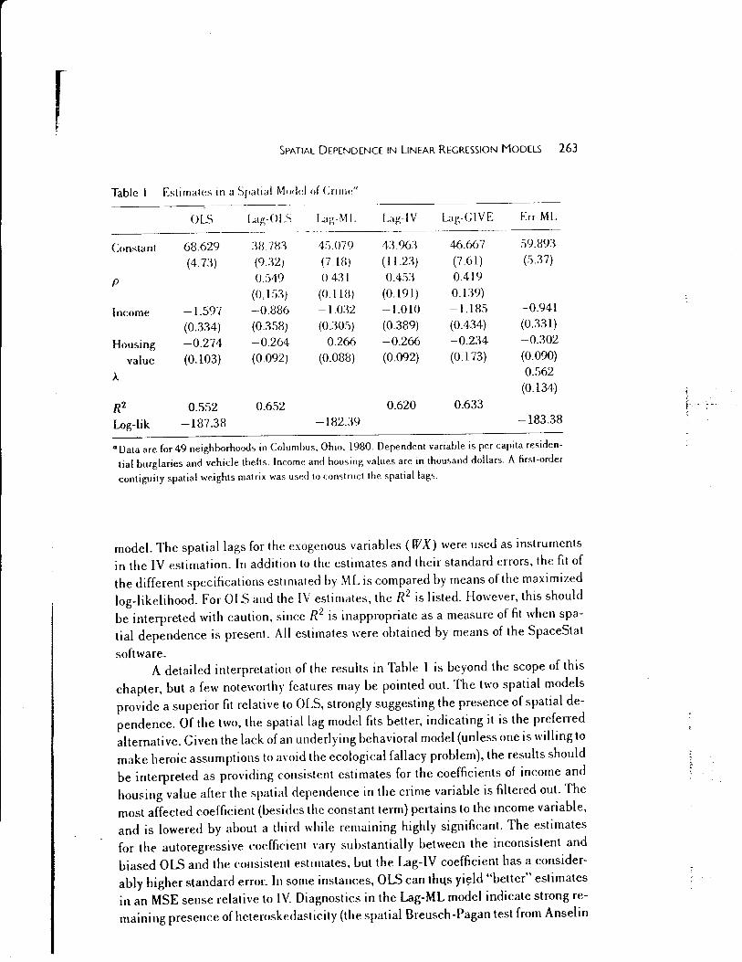
Table I Estimates in a Spatial Modd of <:nnw"

OLS Lag-OLS Lag-ML Lag- IV Ltg-GIVE Err-ML

Constant 68.629 :~8. 781 4.'i.079 4:).%:~ 46.667 59.891

(4.73) (9.:tZJ (7.18) (112:~) (7.61) (5.37)

p 0.549 0.4:{ I 0.4:>:{ 0.419

(0.151) (0.118) (0.191) 0.139)

Income -1.597 -0.886 -l.o:12 -l.OlO -l.l85 -0.941

(0.334) (0.3.'13) (030.'i) (0.389) (0.434) (0331)

Housing -0.274 -0.264 -0.266 -0.266 -0.234 -0.302

value (0.103) (0.092) (0.088) (0.092) (0.173) (0.090)

>.. 0.562 (0.134)

R2 0.552 0.652 0.620 0.633

Log-lik -187.38 -182.39 -183.38

a Data are for 49 neighborhoods in Columbus, Ohio, 1980. Dependent variable is per capita residen­

tial burglaries and vehicle thefts. Income and housing values are in thousand dollars. A first-order

contiguity spatial weights matrix was used to construct the spatial lags.

model. The spatial lags for the exogenous variables (WX) were used as instruments in the IV estimation. In addition to the estimates and their standard errors, the fit of the different specifications estimated by ML is compared by means of the maximized log-likelihood. For OLS and the IV estimates, the R2 is listed. However, this should be interpreted with caution, since R2 is inappropriate as a measure of fit when spa­tial dependence is present. All estimates were obtained by means of the SpaceStat

software. A detailed interpretation of the results in Table l is beyond the scope of this

chapter, but a few notew01thy features may be pointed out. The two spatial models provide a superior fit relative toOLS, strongly suggesting the presence of spatial de­pendence. Of the two, the spatial lag model fits better, indicating it is the preferred alternative. Given the lack of an underlying behavioral model (unless one is willing to make heroic assumptions to a,·oid the ecological fallacy problem), the results should be interpreted as providing consistent estimates for the coefficients of income and housing value after the spatial dependence in the crime variable is filtered out. The most affected coefficient (besides the constant term) pertains to the income variable, and is lowered by about a third while remaining highly significant. The estimates for the autoregressive coefficient vary substantially between the inconsistent and biased OLS and the consistent estimates, but the Lag-IV coefficient has a consider­ably higher standard error. In some instances, OLS can tllltS yi~ld "better" estimates in an MSE sense relative to IV. Diagnostics in the Lag-ML model indicate strong re­maining presence of hcteroskedast icity (the spatial Breusch-Pagan test from Ansel in

264 ANSELIN AND BERA

l98Ba, p. 123, yields a highly significant value of 25.35, p < 0.0000 l ). The robust

Lag-GIVE estimates support the importance of this effect: the estimate for the au­

toregressive parameter is quite close to the ML value while obtaining a significantly

smaller standard error relative to both OLS and the nonrobust IV. Moreover, the es­

timate for the Housing variable is no longer significant. This again illustrates the

complex interaction between heterogeneity and spatial dependence.

IV. TESTS FOR SPATIAL DEPENDENCE

As it happened in the mainstream econometrics literature, the initial stages of de­

velopment in spatial econometrics were characterized by an emphasis on estima­

tion. As discussed in the last section, Cliff and Ord (1973) and others formulated

the maximum likelihood approach which goes to back to work of Whittle {1954). In

mainstream econometrics, the test for serial correlation developed by Durbin and Watson (1950, 1951) was the first explicit specification test for the regression model.

It has gained widespread acceptance since its inception. However, routine testing for other specifications {such as homoskedasticity, normality, exogeneity, and func­tional form) did not take prominence until the early eighties. A major breakthrough

was the rediscovery of the Rao (194 7) score (RS) test (known as the Lagrange multi­

plier test in econometrics). The RS test became very popular due to its computational

ease compared to the other two asymptotically "equivalent" test procedures, namely

the likelihood ratio (LR) and Wald (W) tests (see Godfrey 1988 and Bera and Ullah

1991).

In a similar fashion, the origins of specification testing in spatial econometrics

can be traced back to Moran's (1,950a, 1950b) test for autocorrelation. This test laid

in obscurity until it was revived by Cliff and Ord (1972). It received further impetus

by Burridge (1980) as an RS test. However, the early spatial econometrics literature

on testing was dominated by the Wald and LR tests (for example, see Brandsma and

Ketellapper 1979a, 1979b; Anselin 1980). Since the latter require the estimation of

the alternative model by means of nonlinear optimization (as discussed in Section

III), the advantages of basing a test on the least-squares regression of the null model,

offered by the RS test, were quickly realized. During the last 15 years, a number of

such tests were developed (see Anselin 1988a, 1988c).

Although mainstream econometrics and spatial econometrics literature went

through similar developments in terms of specification testing, the implementation

of the tests in spatial models turns out to be quite different from the standard case.

For example, most of the RS specification tests cannot be written in the familiar

"N R2" form (where R2 is a coefficient of determination) nor they can be computed

by running any artificial regression. In addition, the interaction between spatial lag

dependence and spatial error dependence in terms of specification testing is stronger

and more complex than its standard counterpart. There are, however, some common

SPATIAL DEPENDENCE IN LINEAR REGRESSION MODELS 265

threads. As in the standard case, most of the tests for dependence in the spatial model can be constructed based on the OLS residuals. In our discussion we will em­

phasize the similarities and the differences between specification testing in spatial

econometric models and the standard case. We start the remainder of the section with a discussion of Moran's I statistic

and stress its close connection to the familiar Durbin-Watson test. Moran's I was

not developed with any specific kind of dependence as the alternative hypothesis,

although it has been found to have power against a wide range of forms of spatial dependence. We next consider a test developed in the same spirit by Kelejian and Robinson (1992). This is followed by a focus on tests for specific alternative hypoth­esis in the form of either spatial lag or spatial error dependence. Tests for these two kinds of autocorrelations are not independent even asymptotically, and their sepa­rate applications when other or both kinds of autocorrelations are present will lead to unreliable inference. Therefore, it is natural to discuss a test for joint lag and er­ror autocorrelations. However, the problem with such a test is that we cannot make any specific inference regarding the exact nature of dependence when the joint null hypothesis is rejected. One approach to deal with this problem is to test for spa­tial error autocorrelation after estimating a spatial lag model, and vice versa. This, however, requires ML estimation, and the simplicity of tests based on OlS residuals is lost. We therefore consider a recently developed set of diagnostics in which the OlS-based RS test for error {lag) dependence is adjusted to take into account the

local presence of lag (error) dependence (Anselin et al. 1996). We then provide a brief review of the small-sample properties of the various tests. Finally, the section

is closed into a discussion of implementation issues and our illustrative example of

the spatial model of crime.

A Moran's I Test

Moran's (l950a, l950b) /test was originally developed as a two-dimensional analog

of the test of significance of the serial correlation coefficient in univariate time series.

Cliff and Ord (1972, 1973) formally presented Moran's I s_tatistics as

N (e'We) I= So Te

(42)

where e = y- Xi] is a Yector of OlS residuals, i3 =(X' X)-i X'y, W is the spatial

weights matrix, N is the number of observations, and So is a standardization factor

equal to the sum of the spatial weights, Li Lj Wij· For a row~standardized weights matrix W, So simplifies toN (since each row sum equals 1) and _the statistic becomes

e'We 1=­

e'e (43)

Moran did not derive the statistic from any basic principle; instead, it was suggested

as a simple test for correlation between nearest neighbors which generalized one

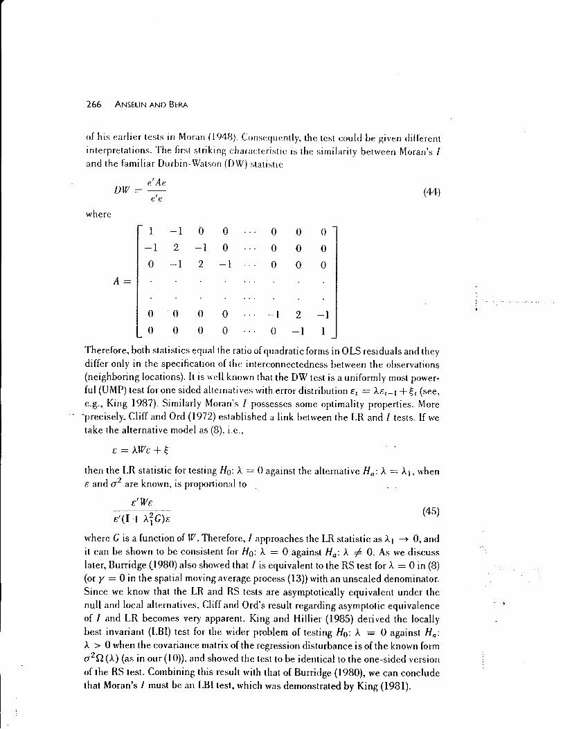
266 ANSELIN AND SERA

of his earlier tests in Moran (l948). Cons{~quently, the test could be ~ivcn different

interpretations. The first striking characteristic is the similarity between Moran's I and the familiar Durbin-Watson (DW) statistic

e'Ae DW= (44)

e'e

where

I -I 0 0 0 0 0

-I 2 -I 0 0 0 0

0 -I 2 -I 0 0 0

A=

0 0 0 0 -1 2 -1

0 0 0 0 0 -1 I

Therefore, both statistics equal the ratio of quadratic forms in 0 lS residuals and they

differ only in the specification of the interconnectedness between the observations (neighboring locations). It is well known that the OW test is a uniformly most power­

ful (UMP) test for one sided alternatives with error distribution Et = AEt-1 +~t (see, e.g., King 1987). Similarly Moran's I possesses some optimality properties. More

· ·precisely, Cliff and Ord (1972) established a link between the LR and I tests. If we take the alternative model as (8), i.e.,

£=AWE+~

then the LR statistic for testing Ho: A = 0 against the alternative Ha: A= At, when £ and CI

2 are known, is proportional to

£1W£

£'(1 +A~ G)£ (45)

where G is a function of W. Therefore, I approaches the LR statistic as A 1 --;. 0, and

it can be shown to be consistent for Ho: A = 0 against Ha: A =/::. 0. As we discuss

later, Burridge (1980) also showed that I is equivalent to the RS test for A = 0 in (8) (or y = 0 in the spatial moving average process (13)) with an unsealed denominator.

Since we know that the LR and RS tests are asymptotically equivalent under the

null and local alternatives. Cliff and Ord's result regarding asymptotic equivalence

of I and LR becomes very apparent. King and Hillier (1985) derived the locally

best invariant (LBI) test for the wider problem of testing Ho: A = 0 against Ha: A > 0 when the covariance matrix of the regression disturbance is of the known form

CI2 Q('A) (as in our (10)). and showed the test to be identical to the one-sided version

of the RS test. Combining this result with that of Burridge (1980), we can conclude

that Moran's I must be an LBI test, which was demonstrated by King (1981).

SPATIAL DEPENDENCE IN LINEAR REGRESSION MODELS 267

In practice the lest is implemented on the basis of an asymptotically normal

standardizeJ z-value, obtained by subtracting the expected value and dividing by

the standard deviation. One advantage of statistic like I is that under flo : A = 0

and normality of E, e' e is distributed as central x2. Cliff and Ord (1972) exploited

this to derive the first two moments as

tr(MW) E (I) = _N ___ K_ (46)

and

tr(MWMW') + tr(MW)2 + {tr(MW)} 2 2 V(l) = - [£(1)]

(N - K)(N - K + 2) (47)

where M = [ - X (X' X) - 1 X', and W is a row-standardized weights matrix.

It is possible to develop a finite-sample-bound test for I following Durbin and

Watson (1950, 1951). However, for I, we need to make the bounds independent of not

only X but also of the weight matrix W. This poses some difficulties. Tiefelsdorf and

Boots (1995), using the results of Imhof (1961) and Koerts and Abrahamse (1968),

showed that exact critical values of I can be computed by numerical integration.

They first expressed I in terms of the eigenvalues Y1· yz, ... , YN-K of MW, other

than the K zeros, and N- K independent N(O, 1) variables 81, 82, ... , 8rv-K; more

specifically,

N-K l\'-K

I = L Yi8I I L 8f (48)

i=l i=l

Then

Pr(l :5 /oiHo) = Pr (~ (y,- lo)Oi :5 OIHo) (49)

Note that L~~~K (Yi - lo)8f is a weighted sum of (N - K) X~ variables. Imhof's

method simplifies the probability in (49) to

where

l l 100 sin{a(u)}

Pr(/ < lolHo) = - - -- 2 JT o ub(u) du

l N-K

a(u) =- "arctan{(Yi - lo)u} 2~

i=1

!\'-K

b ( u) = [ l + ( y i - /o) u ] n 2 2 1/4

i=l

(50)

268 ANSEUN AND BERA

The integral in (SO) can be evaluated by numerical integration (for more on this, see

Tiefelsdorf and Boots 1995). It is instructive to note that the computation of exact critical values of the DW

statistic involves the same calculations as for Moran's I except that the y, is the eigenvalues of MA, where A is the fixed matrix given by in (44). Even with the recent dramatic advances in computer technology, it will take some time for practitioners to use the above numerical integration technique to implement Moran's /test.

B. Kelejian-Robinson Test

The test developed by Kelejian and Robinson (1992) is in the same spirit of Moran's I in the sense that it is not based on an explicit specification of the generating process of the disturbance term. At the same time the test does not require the model to be linear or the disturbance term to be normally distributed. Although the test does not attempt to identify the cause of spatial dependence, Kelejian and Robinson (1992) made the following assumption about spatial autocorrelation:

(S l)

where Zij is l by q vector which can be constructed from the independent variables X, a is q by l vector of parameters, and i, j are contiguous in the sense that they are neighbors in a general spatial "ordering" of the observations. The null hypothesis of

no spatial correlation can be tested by Ho :a = 0 in (51). For a given sample of size N, let C denote hN by l vector <Yi/s which are not

zero fori < j. Therefore, a test for a = 0 can be achieved by running a regression of Con the observation matrix Z which is of dimension hN by q consisting of Zij values. Since we do not obser•e the elements of C, they are replaced by the cross product of OLS residuals, eiej. The resulti1_1g hN by l vector is denoted by C. The test is based

on y = (Z'Z)-1 Z'C and is given by

(52)

where o-4 is a consistent estimator of o-4. For example, we can use [ e' ej Nf or ( C -Zy)'(C - Zy)fhN for a4 • Under Ho : a = 0, KR ._!!. X~ (central chi-square

with q degrees of freedom), where ~ denotes convergence in distribution. Putting y = (Z' Z) -I Z' C, KR can be expressed as

C'Z(Z'Z)- 1Z'C KR=----­o--t

(53)

Since for the implementation of the test we need the distribution only under the null hypothesis, it is legitimate to replace o-4 by a consistent estimate under a = 0.

'

SPATIAL DEPENDENCE IN LiNEAR REGRESSION MODELS 269

/' I' Note that under Ho, C''C'/hN ---+ a\ where --+ means convergence in probability. Therefore, an asymptotically equivalent form of the u~st is

(54)

which has the familiar N R2 form. Here R2 is the uncentered coefficient of determi­nation of Con Z and hN is the sample size of this regression.

It is also not difficult to see an algebraic connection between K Rand Moran's /_ From (43)

2 (e'We) 2

I=--­( e' e )2

Using (53), we can write

(55)

(56)

where PiJ are the elements of Z(Z'Z)- 1Z'_ Given that C;'s contain terms like e~;e,, k < l, it appears that the 12 and KR statistics have similar algebraic structure.

C Tests for Spatial Error Autocorrelation

In contrast to the earlier two tests, the alternative hypothesis is now stated explicitly through the data generating process of E as in (8), i.e.,

E =AWE+~

and we test A = 0. All three general principles of testing, namely LR, W, and RS can be applied. Out of the three. the RS test as described in Rao (194 7) is the most convenient one to use since it requires estimation only under the null hypothesis. That is, the RS test can be based on the OLS estimation of the regression model (7). Silvey (1959) derived the RS test using the Lagrange multiplier(s) of a constrained

optimization problem. Burridge (1980) used Sil\'ey's form to test A = 0, although the Rao's score

form, namely

(57)

270 ANSELIN AND BERA

is more popular and much easier to us(~. In (S7), d{G) = oL(8)jo8 is the score

vector, I(8) = -E[o2L(8)/o((})()((;l)'l is the information matrix, L(G) is the log­

likelihood function, and (j is the (f'Sirir-tf'rf (under the tested hypothesis) maximum

likelihood estimator of the paramf:tn vector G. For the spatial error autocorrelation

modele = ({3', a 2 , A.)' and the log-likelihood function is given in (34). The test is

essentially based on the score with respect to A., i.e., on

aL d;.. =­a A.

(58)

We can immediately see the connection of this to Moran's I statistic. After computing

I(8) under Ho, from (36), we have the test statistic

lf. [e'Weja2f RS;..=- = ----

T T (59)

where T = tr[(W' + W) W]. Therefore, the test requires only OLS estimates, and

. under H0 , RS;.. ~ xi. It is interesting to put W = wr (Section lLE) and obtain

T = N -1 and RS;.. = (N -1)F where).= Lr e1e1-t/ Lt e~_ 1 in the time-series context. Burridge (1980) derived the RS test (59) using the estimates of the Lagrange

multiplier following Silvey (1959). The Lagrangian function for this problem is

(60)

where JL is the associated Lagrange multiplier. From the first-order conditions, we

have

=0 0,[1

Le.,

(61)

and this results in the same statistic RS;.. _ A striking feature of the RS test is its invariance to different alternatives (for

details, see Bera and McKenzie 1986)_ The RS test uses the slope aL;ae at(} = B. and there may be many likelihood functions (models) which have the same slope at (j_ If we specify the alternative hypothesis as a spatial moving-average process (13) and

test Ho : y = 0. we obtain the same Rao's score statistic RS;... Therefore, RS;.. will

be locally optimal for both autoregressive and moving-average alternatives. But this

also means that when the null hypothesis is rejected, the test does not provide any

guidance regarding the nature of the disturbance process, even when other aspects

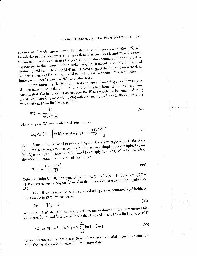
-SPATIAL DEPENDENCE IN LINEAR REGRESSION MODELS 271

of the spatial model are resolved. This also raises the question whether RS). will be inferior to other asymptotically equivalent tests such as LR and W, with respect to power, since it does not use the precise information contained in the alternative

hypothesis. In the context of the standard regression model, Monte Carlo results of Godfrey (1981) and Sera and McKenzie (1986) suggest that there is no setback in the performance of RS test compared to the LR tesL In Section IVG, we discuss the

finite sample performance of RS A A!nd other tests. Computationally, the W and LR tests are more demanding since they require

ML estimation under the alternative, and the explicit forms of the tests are more

complicated. For instance, let us consider theW test which can be computed using the ML estimate 5. by maximizing (34) with respect to {3, a

2, and A. We can write the

W statistic as (Anselin 1988a, p. 104)

)_2 ws),_ = --- A

AsyVar(A)

where AsyVar (5.) can be obtained from (38) as

(62)

(63)

For implementation we need to replace A by 5. in the above expression. In the stan­

dard time-series regression case the results are much simpler. For example, AsyVar [a2 , A} is a diagonal matrix and AsyVar(.>-) is simply (1 - A

2)j(N - 1). Therefore

the \Vald test statistic can be simply written as

T (N- l)F ws),_ = 1- ;_z

(64)

Note that under A = 0, the asymptotic variance (1- A 2)/(N- 1) reduces to lj(N-

1), the expression for AsyVar(l) used in the time series case to test the significance

of A. The LR statistic can be easily obtained using the concentrated log-likelihood

function Lc in -(37). We can write (65)

where the "hat" denotes that the quantities are evaluated at the unrestricted ML estimates~. iP, and 5.. It is easy to see that LR). reduces to (Anselin 1988a, p. 104)

N

LRA = N[lna2 -lna2]+2 Lln(1- lw;) (66)

i=l

The appearance of the last term in (66) differentiate the spatial dependence situation

from the serial correlation case for time-series data.

.. ·~~,:.:_ . -

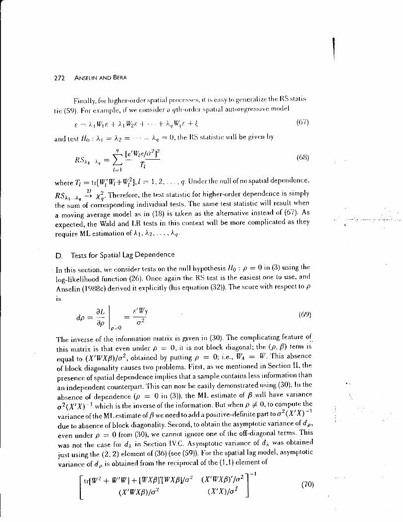
272 ANSELIN AND BERA

Finally, for higher-order spatial proccss<~s, it is easy to generalize the f\S statis­tic (59). For example, if we consider a qth-order spatial autoregressive model

E = )q w, E + )q W2E + ... + Aq W,E + ~ (67)

and test Ho: AJ = A.2 = ···=).'I= 0, theW) statistic will be given by

q [e'W/eja2 f RSAJ Aq = L T.

1=1 I

(68)

where T1 = tr[ W/ WI+ ffi?J, l = l, 2, ... , q. Under the null of no spatial dependence,

RS A., ... A." ~ X~· Therefore, the test statistic for higher-order dependence is simply the sum of corresponding individual tests. The same test statistic will result when a moving average model as in (18) is taken as the alternative instead of (67). As expected, the Wald and LR tests in this context will be more complicated as they

require ML estimation of At, A.2, ... , Aq·

D. Tests for Spatial Lag Dependence

In this section, we consider tests on the null hypothesis Ho : p = 0 in (3) using the log-likelihood function (26). Once again the RS test is the easiest one to use, and Anselin (l988c) derived it explicitly (his equation (32)). The score with respect top

IS

aL dp=­op

p=O

E'Wy

a2 (69)

The inverse of the information matrix is given in (30). The complicating feature of. this matrix is that even under p = 0, it is not block diagonal; the (p, /3) term is equal to (X'WXf3)ja2, obtained by putting p = 0; i.e., WA = W. This absence of block diagonality causes two problems. First, as we mentioned in Section II, the presence of spatial dependence implies that a sample contains less information than an independent counterpart. This can now be easily demonstrated using (30). In the absence of dependence (p = 0 in (3)), the ML estimate of f3 will have variance a 2(X' X)- 1 which is the inverse of the information. But when p =/= 0, to compute the variance of the ML estimate of f3 we need to add a positive-definite part to a 2(X' X) -I due to absence of block diagonality. Second, to obtain the asymptotic variance of dp, even under p = 0 from (30), we cannot ignore one of the off-diagonal terms. This was not the case for dA. in Section IV.C. Asymptotic variance of dA. was obtained just using the (2, 2) element of (36) (see (59)). For the spatial lag model, asymptotic

variance of d P is obtained from the reciprocal of the ( l ,l) element of

[

ti1W 2 + W'W] + [WXf3}'[WXf3]ja2

(X'WX{3)ja2

(X'WX/3)'/~2 ]-l (X' X)ja2

(70)

l I

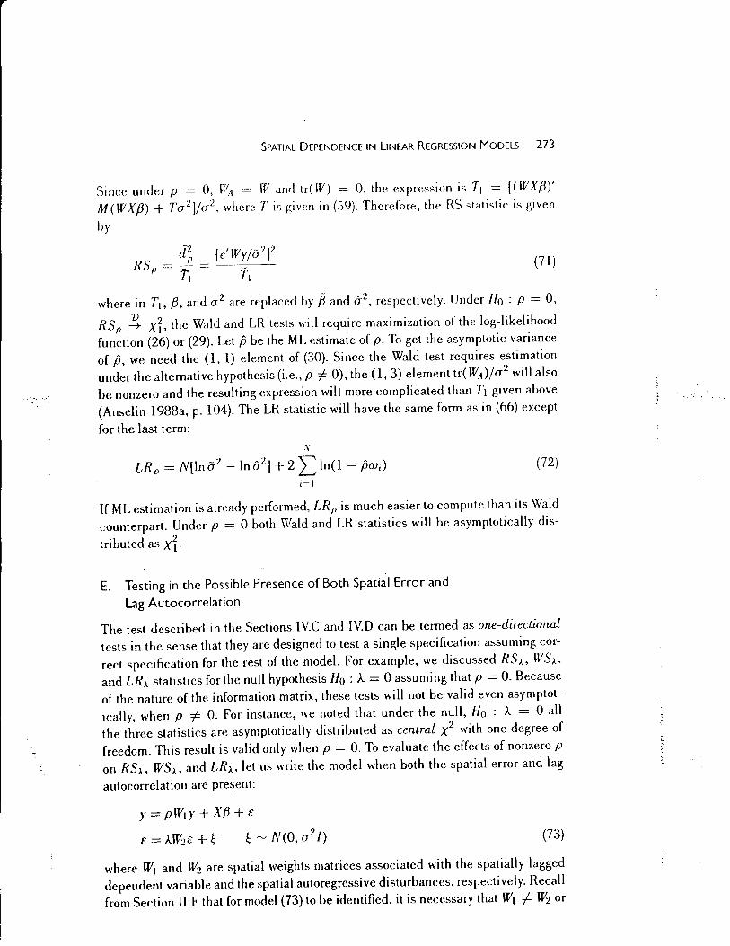
SPATIAL DEPENDENCE IN liNEAR REGRESSION MODELS 273

Since under p = 0, WA = wand tr(W) = 0, the expression is r, = [(WX,B)' M(WX,B) + Ta 2 J!a2 , where Tis giVf:n in (S9). Therefore, the RS statistic is given

by

J~ [e'Wyja-2]2 RSp = -::--- ----

T1 t, (71)

where in f 1, ,8, and a 2 are replaced by~ and a- 2, respectively. Under Ho : p = 0,

RS P ~ xi, the Wald and LR tests will require maximization of the log-likelihood

function (26) or (29). Let p be the ML estimate of p. To get the asymptotic variance

of{>, we need the (l, 1) element of (30). Since the Wald test requires estimation

under the alternative hypothesis (i.e., p ::/= 0), the (l, 3) element tr(WA)fa2

will also

be nonzero and the resulting expression will more complicated than Tt given above

(Anselin l988a, p. 104). The LR statistic will have the same form as in (66) except

for the last term:

X

LRp = N[lna2 -lnG-2]+2 Lln(l- f>wi) i=l

(72)

If ML estimation is already performed, LRp is much easier to compute than its Wald

counterpart. Under p = 0 both Wald and LR statistics will be asymptotically dis-

tributed as xi.

E. Testing in the Possible Presence of Both Spatial Error and

Lag Autocorrelation

The test described in the Sections IV.C and IV.D can be termed as one-directional tests in the sense that they are designed to test a single specification assuming cor­

rect specification for the rest of the model. For example, we discussed RS).., WS>... and LR>.. statistics for the null hypothesis Ho : A = 0 assuming that p = 0. Because

of the nature of the information matrix, these tests will not be valid even asymptot­

ically, when p =/= 0. For instance, we noted that under the null, Ho : A = 0 all

the three statistics are asymptotically distributed as central x2 with one degree of

freedom. This result is valid only when p = 0. To evaluate the effects of nonzero p on RS>.., WS>... and LR>... let us write the model when both the spatial error and lag

autocorrelation are present:

J = pW,y + X,B + E

£ = AW2E + ~ ~ "' N (0, a 2/) (73)

where W1 and W2 are spatial weights matrices associated with the spatially lagged

dependent variable and the spatial autoregressive disturbances, respectively. Recall

from Section II.F that for model (73) to be identified, it is necessary that Wt =/= W2 or

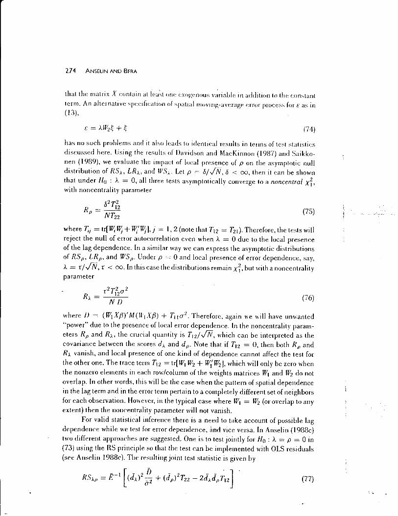
2 7 4 ANSELIN AND BERA

that the matrix X contain at l(:a~t one exog<:nous variable in addition to the constant

term. An alternative specification of spatial moving-average error process for£ as in (13),

(71)

has no such problems and it also leads to identical results in terms of test statistics

discussed here. Using the results of Davidson and MacKinnon ( 1987) and Saikko­

nen (1989), we evaluate the impact of local presence of p on the asymptotic null

distribution of RS;.., LR;_, and WS;_. Let p = 8/.Jili, 8 < oo, then it can be shown

that under Ho : A = 0, all three tests asymptotically converge to a noncentral xf, with noncentrality parameter

82T2 R - __ 12 p-

NT22 (75)

where Tij = trfJlli Jfj + ~'lfj ], j = 1, 2 (note that T12 = TzJ). Therefore, the tests will reject the null of error autocorrelation even when A = 0 due to the local presence

of the lag dependence. In a similar way we can express the asymptotic distributions

of RS P' LRp, and WS p· Under p = 0 and local presence of error dependence, say,

A = rj.../N, r < 00. In this case the distributions remain xi, but with a noncentrality parameter

r2T2 a2 R _ 12 ;..- ND (76)

where D = (WtX,B)'M(WtX,B) + Ttta2. Therefore, again we \\ill have unwanted

"power" due to the presence of local error dependence. In the noncentrality param­

eters Rp and R;.., the crucial quantity is Ttz!.Jili, which can be interpreted as the

covariance between the scores d1.. and dp. Note that if T12 = 0, then both Rp and

R;.. vanish, and local presence of one kind of dependence cannot affect the test for

the other one. The trace term T12 = tr[Wt W2 + W(Wz], which will only be zero when

the nonzero elements in each row/column of the weights matrices Wt and W2 do not

overlap. In other words, this will be the case when the pattern of spatial dependence

in the lag term and in the error term pertain to a completely different set of neighbors

for each observation. However, in the typical case where W1 = W2 (or overlap to any extent) then the noncentrality parameter will not vanish.

For valid statistical inference there is a need to take account of possible lag

dependence while we test for error dependence, and vice versa. In Ansel in ( l988c) two different approaches art> suggested. One is to test jointly for Ho : A = p = 0 in

(73) using the RS principle so that the test can be implemented with OLS residuals

(see Ansel in l988c). The resulting joint test statistic is given by

(77)

SPATIAL DEPENDENCE IN LINEAR REGRESSION MODELS 275

where f: = (Dja 2 )Tzz- (T,z)2. Note that this JOint test not only depends on d,_ and dfl but also on their interaction factor with a coefficient T12- Expression (77) ap­

pears to be somewhat complicated but can be computed quite easily usin~ only OLS residuals. Also the expression simplifies greatly when the spatial weights matrices

W1 and Wz are assumed to be the same which is the case in most applications. Under

W1 = Wz = W, Ttl= Tzt = T22 = T = tr[(W' + W)W], and (77) reduces to

(78)

Under Ho : A. = p = 0, RSAp will converge to a central x2 with two degrees of

freedom. Because of this two degrees of freedom, the statistic will result in loss of

power compared to the proper one-directional test when only one of the two forms

of misspecification is present. To see this consider the presence of only A.= rj./N, with p = 0. In this case the noncentrality parameter for both RSA and RSAp is

the same r 2 NT. Due to the higher degrees of freedom of the joint test RS J..p, we

can expect some loss of power (Dasgupta and Perlman 1974). Another problem

with RSAp is that since it is an omnibus test, if the null hypothesis is rejected,

it is not possible to infer whether the misspecification is due to lag or error depen-

dence. A second approach is to carry out an RS test for one form of misspecification in

a model where the other form is unconstrained. For example, this consists of testing

the null hypothesis Ho : A. = 0 in the presence of p, i.e., based on the residuals

of a maximum likelihood estimation of the spatial lag modeL The resulting statistic

RSAIP is given as

(79)

where the "hat" denotes quantities are evaluated at the maximum likelihood esti­

mates of the parameters of the model Y = pWt)' + X{J + ~ obtained by means

of nonlinear optimization. In (79) T21 A stands for tr( Wz W1 A-t + w; Wt A-t], with

A = I - p Wt- Under Ho : A. = 0, RS>..fp will converge to a central x2

with one

degree of freedom. Similarly, an RS test can be developed for Ho : p = 0 in the

presence of error dependence (Anselin et aL 1996). This test statistic can be writ-

ten as

(80)

where tis a vector of residuals in the ML estimation of the null model with spatial

AR errors,}'= X{J + (l- A.Wz)- 1 ~ with()= ({3'. A., a2)'. and B = l- >..Wz. The

terms in the denominator of (80) are

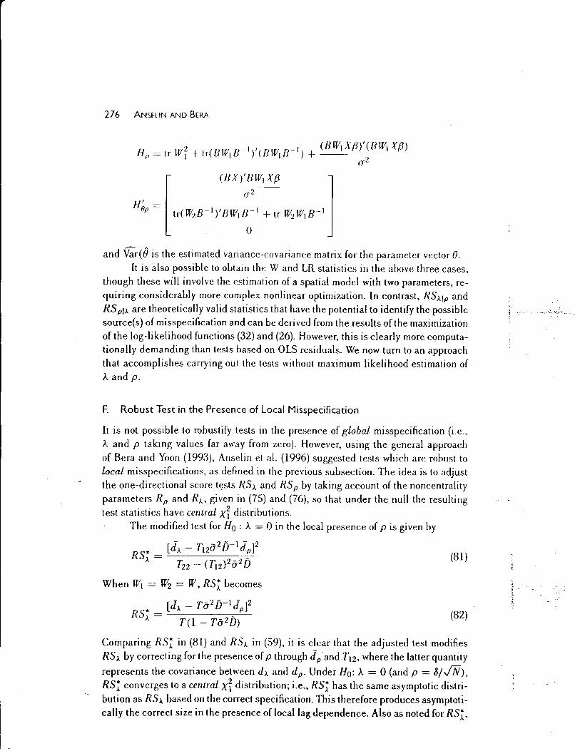
2 7 6 ANSELIN AND BERA

( BW Xf3)'(BW Xf3) If p = t r w i + t r( 8 WI tr I ) I ( H WI rr I ) + I 2 I

tr(W2B- 1)'BW1B- 1 +tr W2W1B- 1

0

(J

and fu(B is the estimated variance-covariance matrix for the parameter vector 8. It is also possible to obtain the W and LR statistics in the above three cases,

though these will involve the estimation of a spatial model with two parameters, re­

quiring considerably more complex nonlinear optimization. In contrast, RS>..Jp and

RS pi>.. are theoretically valid statistics that have the potential to identify the possible source(s) of misspecification and can be derived from the results of the maximization of the log-likelihood functions (32) and (26). However, this is clearly more computa­

tionally demanding than tests based on OLS residuals. We now turn to an approach

that accomplishes carrying out the tests without maximum likelihood estimation of )._and p.

F. Robust Test in the Presence of Local Misspecification

It is not possible to robustify tests in the presence of global misspecification (i.e.,

)._ and p taking values far away from zero). However, using the general approach

of Bera and Yoon (1993), Anselin et aL (1996) suggested tests which are robust to

local misspecifications, as defined in the previous subsection. The idea is to adjust

the one-directional score_t~sts RS). and RSp by taking account of the noncentrality

parameters Rp and R>., given in (75) and (76), so that under the null the resulting test statistics have central X~ distributions.

The modified test for Ho : A = 0 in the local presence of p is given by

- 2- I - 2 * [d>.. - T12(J D- dp]

RSA = . -T22 - (Ttz)2(T2 D

(81)

When W1 = Wz = W, RS~ becomes

[J - T(J2jj-IJ f RS* = A - p

A T(l - Tjj2D) (82)

Comparing RS~ in (81) and RS). in (59), it is clear that the adjusted test modifies

RS'A by correcting for the presence of p through JP·and T12, where the latter quantity

represents the covariance between d). and dp. Under H0 : )._ = 0 (and p = 8/.Jiii),

Rsr converges to a central xi distribution; i.e., RS~ has the same asymptotic distri­

bution as RS>.. based on the correct specification. This therefore produces asymptoti­

cally the correct size in the presence of local lag dependence. Also as noted for Rsr,

' .

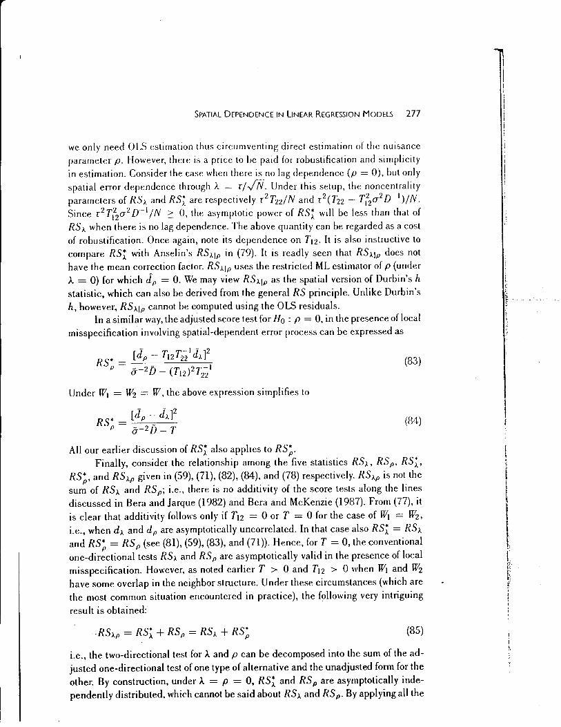
SPATIAL DEPENDENCE IN LINEAR REGRESSION MODELS 277

we only need OLS estimation thus circumventing direct estimation of the nuisance parameter p. However, there is a price to be paid for robustification and simplicity in estimation. Consider the case when there is no lag dependence (p = 0), but only spatial error dependence through A = r/ffi. Under this setup, the noncentrality parameters of RS1.. and RS;. are respectively r2T22/N and r 2(T22 - T1

22a-2D- 1)JN.

Since r 2 T~2a-2 D- 1 IN 2: 0, the asymptotic power of RS1 will be less than that of RSA. when there is no lag dependence. The above quantity can be regarded as a cost of robustification. Once again, note its dependence on T12 . It is also instructive to compare RS1 with Anselin's RS1..1p in (79). It is readly seen that RSA.Ip does not have the mean correction factor. RSI..Ip uses the restricted ML estimator of p (under ).. = 0) for which JP = 0. We may view RSA.Ip as the spatial version of Durbin's h statistic, which can also be derived from the general RS principle. Unlike Durbin's h, however, RS>..lp cannot be computed using the OLS residuals.

In a similar way, the adjusted score test for Ho : p = 0, in the presence of local misspecification involving spatial-dependent error process can be expressed as

- -1 - 2 RS* = [dp- T12T22 d~..]

P o--2[)- (Tt2)2T2~1 (83)

Under W1 = W2 = W, the above expression simplifies to

- - 2 RS* = [dp- d~..]

P o--2[)- T (84)

All our earlier discussion of RS1 also applies to RS;. Finally, consider the relationship among the five statistics RSA., RSp, RS;,

RS;, and RS>..p given in (59), (71), (82), (84), and (78) respectively. RSA.p is not the sum of RS>.. and RSp; i.e., there is no additivity of the score tests along the lines discussed in Bera and Jarque (1982) and Bera and McKenzie (1987). From (77), it is clear that additivity follows only if T12 = 0 or T = 0 for the case of W1 = W2, i.e., when d1.. and dp are asymptotically uncorrelated. In that case also RS1 = RSA. and Rs; = RS P (see (81), (59), (83), and (71)). Hence, forT = 0, the conventional one-directional tests RS >.. and RS p are asymptotically valid in the presence of local misspecification. However, as noted earlier T > 0 and T12 > 0 when W1 and W2 have some overlap in the neighbor structure. Under these circumstances (which are the most common situation encountered in practice), the following very intriguing

result is obtained:

(85)

i.e., the two-directional test for A and p can be decomposed into the sum of the ad­justed one-directional test of one type of alternative and the unadjusted form for the other. By construction, under A = p = 0, RS1 and RS P are asymptotically inde­pendently distributed, which cannot be said about RS>.. and RSp. By applying all the

278 ANSELIN AND BERA

unadjusted and adjusted tests and exploiting the result (RS), it is possible ·to identify the exact nature of dependence in practice (Anselin et al. 1996). Finally, we should mention that because of the complexity of the Wald and LR tests, 11 is not possible to derive their adjusted versions that would be valid under local misspecification. Of course, it is not computationally prohibitive to obtain these tests after the joint estimation of both A. and p.

G. Small Sample Properties

We have covered a number of procedures for testing spatial dependence. For ease of implementation, we have emphasized Rao's score test which in many cases can be computed based on the OLS residuals. As we indicated, all these tests are of asymp­totic nature; i.e., their justification derives from the presence of very large samples. That is, however, not the case in most applications. The small sample performance of the above tests both in terms of size and power is of major concern to practitioners.

There are only a few papers on the finite sample properties of tests on spatial dependence compared to the vast literature on those for testing for serial correlation for time-series data as summarized in King (1987). Bartels and Hordijk (1977) stud­ied the behavior of Moran's I. However, their focus was on the performance of dif­ferent residuals, and they found that OLS residuals give the best results. Brandsma and Ketellapper (1979b) included the LR test (LRA) in their study, but it performed poorly compared to I. Both these studies were quite limited in terms of a small num­ber of replications, few sample sizes, the use of only one type (irregular) weights matrix and the narrow range of alternative values for the autocorrelation coefficient. A first extensive set of Monte Carlo simulations was carried out by Anselin and Rey {1991), who compared Moran's I to RSA and RSp for different weights matrices and error distributions. In terms of size, the small sample distributions of the statistics corresponded close to their theoretical counterparts, except for the smallest size {N = 25). In terms of power, Moran's I had power against both kinds of depen­

dence, spatial lag and error autocorrelations. RS>.. and RSp had highest power for their respective designated alternatives. These tests were found to possess superior performance, but they fall short of providing a good strategy for identifying the exact nature of dependence.

Anselin and Florax (199Sb) provide the most comprehensive set of simulation results to date. They carried out experiments for both regular (rook and queen) and nonregular weight matrices. single- and multidirectional alternatives, and for differ­ent error distributions, and included all the tests discussed earlier except the Wald and LR tests. The results are too extensi\·e to discuss in detail, and here we provide only a brief summary of the main findings. First, the earlier results of Anselin and Rey ( 1991) were confirmed on the power of I against any form of dependence and the optimality of the RS tests against the alternatives for which they were designed. Second, the specification of the spatial weights matrix impacted the performance of

SPATIAL DEPENDENCE IN LINEAR REGRESSION MODELS 279

all tests, with a higher power obtained in the rook case. Third, as in Anselin and Rey (1991), higher powers were achieved by lag tests relative to tests against error dependence. This is important, since the consequences of ignoring lag dependence are more serious. Fourth, the KR statistic did not perform well. For example, when the errors were generated as lognormal, it significantly over rejected the true null hy­pothesis in all configurations. There are two possible explanations. One is its higher degrees of freedom. Another is that its power depends on the degree of autocorre­lation in the explanatory variables which substitute for the weights matrix (compare (55) and (56)). It is interesting to note that White's (1980) test for heteroskedasticity which is very similar to KR encounters problems of the same type. Fifth, the most striking result is that the adjusted tests RS; and RSp* performed remarkably welL They had reasonable empirical sizes, remaining within the confidence interval in all cases. In terms of power they performed exactly the way they were supposed to. For instance, when the data were generated under p > 0, A = 0, although RS P had the most power, the powers of Rs; was very dose to that of RSp. That is, the price paid for adjustments that were not needed turned out to be small. The real superiority of Rs; was revealed when A > 0 and p = 0. It yielded low rejection frequencies even for A = 0.9. The correction for error depen?~nce in Rs; workedin the right direc­tion when no lagged dependence was present for all configurations. When p > 0, the power function of Rs; was seen to be almost unaffected by the values of A, even for those far away from zero (global misspecification). For these alternatives RS;._p also had good power, but could not point to the correct alternative when only one kind of dependence is present. RS~ also performed well though not as spectacularly as Rs;. The adjusted tests thus seem more appropriate to test for lag dependence in the presence of error correlation than for the reverse case. Again, this is impor­tant since ignoring lag dependence has more severe consequences. Based on these results Ansel in and Florax (l995b) suggested a simple decision rule. When RS p is more significant than RS;._, and Rs; is significant while RS~ is not, a lag depen­dence is the likely alternative. In a similar way presence of error dependence can be identified through RS;. Finally, the finite-sample performance of tests against higher-order dependence RS;._ 1;._ 2 (see (68)) and the joint test RS;._p were satisfactory, although these type of tests pro\"ide less insightful guidance for an effective specifi­cation search. For joint and higher-order alternatives, these tests are optimal, and in practice they should be used along with the unadjusted and adjusted one-directional tests.

H. Operational Implementation and Illustration

As is the case for the estimation of spatial regression models, specification tests for spatial dependence are notably absent from econometric software, with the exception of SpaceStat (Anselin l992b. 1995). Moreover, as pointed out, these tests cannot be obtained in the usual N R2 format, which lends itself to straightforward implemen-

280 ANSEUN AND BERA

tation by means of auxiliary or augmented regressions. The closest to this situation is the Kelejian-Robinson test (S4), provided one has an easy way to select the pairs of neighboring data points from the data. Typically, specification tests for spatial de­

pendence must be implemented expl icitly.either by writing special-purpose software or by taking advantage of macros in econometric and statistical software. As in max­imum likelihood estimation, the size of the weights matrix may be a constraint when the number of observations is large. This is particular! y the case for Moran's I, where several operations are involved in the computation of the expected value and vari­ance (46) and (47). Examples of the implementation of this test for small data sets in standard econometric software are given in Anselin and Hudak {1992) and Ansel in et al. {1993b), for Shazam, Rats and Limdep, among others.

Given their importance for applied work, we now briefly describe implemen­tation strategies for the RS tests for spatial error and spatial lag autocorrelation, RS.J.. (59) and RSp (71). First, note that the squared expression in the numerator equals N times a regression coefficient of an auxiliary regression of respectively We on e (in (59)) and Wy or_:~ _e {in {71)). Once the lags are constructed, these coefficients can be obtained using standard software. The denominator in the expressions is slightly more complex. The trace elements T = tr(WW)+ tr(W'W) can easily be seen to -

equal, respectively, L; Lj w;1wji and L; L/W;j)2. When the spatial weights ma­

trix consists of simple row-standardized contiguity weights, each element Wij for a given i equals 1/k;, where k; is the number of neighbors for observation i. Hence,

L; "'I:,j(w;j) 2 = L;O/k;), which can easily be computed. The other trace term

i,. "I:,; "I:,j W 1j. Wji = L;(1/k; HLj 8;j/kj ], where 8ij is a binary variable indicating whether or not Wij # 0. This requ·ires only slighly more work to compute, similar to the sorting needed to establish the neighbor pairs in the Kelejian-Robinson test. !\lost importantly, the trace operations can be carried out without having to store a full matrix in memory, taking advantage of the sparse nature of spatial weights (for technical details, see Anselin 1995). Of course, for symmetric weights, the two traces are equal. In practice, this may occur when all observations are considered to have an equal number of neighbors. as in Pace and Barry (1996). The other term in the denominator of (71) is the residual sum of squares in a regression with WXb (i.e., the sp~tiallags for the predicted values from the OLS regression) on X, which can be

obtained in a straightforward way. To illustrate the various specification tests, we list the results of Moran's I, KR,

and the RS and LR tests for the spatial model of crime in Table 2 (using a slightly dif­ferent notation, most of these results are reported in Table 2, p. 87 of Anselin et al. 1996). All results are Nrt of the standard SpaceStat regression diagnostic output. They reflect a situation that is often encountered in practice: strong significance of Moran's I and KR, as well as of both one-directional RS and LR tests. Clearly, spa­

tial dependence is a problem, although without further investigation it is not obvious which form of spatial dependence is the proper alternative. Convincing evidence is provided by the robust tests RS~ and RS;. While the former is not at all significant,

SPATIAL DEPENDENCE IN LiNEAR REGRESSION MODELS 281

Table 2 Specification Tec,h a~amc,t Spatial Dqwndence"

Estimate.., Tec,l (equatwn number) Yalut: p-value

OLS Moran's I (z-value) (4~) 2.9.S o.om OLS Kelejian-Robinson (S4) 11.:>5 0.009

OLS RS).p {78) 9.44 0.009

OLS R.S). (59) 5.72 0.02

OLS Rsr {82J 0.08 0.78

OLS RSP (7l) 9.~6 0.002

OLS Rs; (84) ~.72 0.05

Lag-ML LRp (72) 9.97 0.002

Lag-ML RS).Ip (79) 0.32 0.57

Err-ML LR). (66) 7.99 0.005

Err-ML RSpl). (80) 1.76 0.18

«Source: From Anselin (1938a, Chap. 12; l992a, Chap. 26; 1995) and

Anselin et al. (1996).

the latter is significant at p slightly higher than 0.05. In other words, the impression of spatial error autocorrelation that may be given by an uncritical interpretation of Moran's I is spurious, since no evidence of such autocorrelation remains after ro­bustifying for spatial lag dependence. Instead, a spatial lag model is the suggested alternative, consistent with the estimation results in Table l.

V. CONCLUSIONS

In our review of methods to deal with spatial dep~ndence in regression analysis, we have emphasized the distinguishing characteristics of spatial econometrics relative to time-series analysis. We highlighted the concept of spatial weights and the as­sociated spatial lag operator which allow for the formal specification of neighbors in space, a much more general concept than its counterpart in time. In the estima­tion of spatial regression models, the maximum likelihood approach was shown to be prevalent and requiring nonlinear optimization of the likelihood function. The simplifying results from serial correlation in time series do not hold and estimation necessitates the explicit manipulation of matrices of dimension equal to the number of observations. Diagnostics for spatial effects in regression models may be based on the powerful score principle, but they do not boil down to simple significance tests of the coefficients in an auxiliary regression, as they do for time series.

The differences between the time domain and space are both puzzling and challenging, in terms of theory as well as from an applied perspective. They are the subject of active research efforts to develop diagnostics for multiple sources of mis-

282 ANSELIN AND BERA

specification, to discriminate betwcf:n hetero~eneity and spatial dependence, and to estimate models for complex forms of interaction in realistic data settmgs. Ex­tensions to the space-time domain and to models for limited dependent variables are patticularly challenging. We hope that our review of the fundamental concepts and basic methods will stimulate others to both apply these techniques as well as to

pursue solutions for the remaining research questions.

ACKNOWLEDGMENTS

We would like to thank Aman Ullah and an anonymous referee for helpful sugges­

tions, and Robert Rozovsky for very able research assistance. We also would like to thank Naoko Miki for her help in preparing the manuscript. However, we retain the responsibility for any remaining errors. The first author acknowledges ongoing support for the development of spatial econometric methods by the U.S. National Sci­

ence Foundation, notably through grants SES 87-21875, SES 89-21385, and SBR 94-10612 as well as grant SES 88-10917 to the National Center for Geographic In­formation and Analysis (NCGIA). The second author acknowledges financial support by the Bureau of Economic and Business Research of the University of Illinois.

REFERENCES

Albert, P. and L. M. McShane~ l99.S). :\Generalized Estimating Equations Approach for Spa­tially Correlated Binary Data: Applications to the Analysis of Neuroimaging Data, Bio-

metrics, SL 627--638. Amemiya, T. (1985). Advanced Econometrics, Harvard University Press, Cambridge. MA. Ancot, J-P., J. Paelinck, and J. Prins (1986). Some New Estimators in Spatial Econometrics,

Economics Letters. 2L 245-249. Anselin. L. (1980), EstimatiDn Methods for Spatial Autoregressive Structures, Regional Sci-

ence Dissertation and Monograph Series 8, Cornell University, Ithaca, NY. Ansel in, L. (1982). A Note on Small Sample Properties of Estimators in a First-Order Spatial

Autoregressive ModeL Environment and Planning A, 14, 1023-1030. Anselin, L. (1988a), Spatial Econometrics: Methods and Models, Kluwer, Dordrecht. Anselin. L. (1988b). Model Validation in Spatial Econometrics: A Review and Evaluation of

Alternative Approaches./nternational Regional Science Review, 11.279-316. Anselin. L. (1988c). Lagrange Multiplier Test Diagnostics for Spatial Dependence and Spatial

Heterogeneity. Ceo graphical Anal_rsis, 20. l-17. Anselin. L. (1990a). Spatial Dependence and Spatial Structural Instability in Applied Re-

gression Analysis. Journal of Regional Science. 30, 185-207. Anselin. L. (l990b). Some Robust Approaches to Testing and Estimation in Spatial Econo-

metrics. Regional Science and Urban Economics. 20. 141-163. Anselin. L. (ed.) (1992a). Space and Applied Econometrics. Special Issue, Regional Science

and Urban Economics. "2.2.

I

l

SPATIAL DEPENDENCE IN LINEAR REGRESSION MODELS 283

Ansdin, L. ( 19921,), Space Stat: A PmKmm for the A1Udysi.1 (1 Spatial Data, National Center for Geographic Information and Analy'"~' Univer;,ity of California, Santa Barbara. CA.

Anselin, L (199.'>), SpaceStat Version UtfJ U1er's Cuide, Regional Research Institute, \\bt

Virginia University, Morgantown, \\-V_ Ansel in, L, A. K. Bera, R. Florax, and M. J _ Yoon ( 1996), Simple Diagnostic Tests for Spatial

Dependence, Regional SCLence and Urban Economics, 26, 77-104. Anselin, Land A. Can (1996), Spatial Effect;, in Models of Mortgage Origination, Paper pre­

sented at the Mid Year AREUEA Conference, Washington, DC, May 28-29. Anselin, L, R. Dodson, and S. Hudak (199:1a), Linking GIS and Spatial Data Analysis in

Practice, Geographical Systems, 1, 3-23. Anselin, L, R. Dodson, and S. Hudak (1993b), Spatial Data Analysis and GIS: Interfacing

GIS and Econometric Software, Technical Report 93-7, National Center for Geographic

Information and Analysis, University of California, Santa Barbara. Anselin, Land R. Florax (eds.) (199Sa), NetL Directions in Spatial Econometrics, Springer­

Verlag, Berlin. Anselin, L. and R. Florax (1995b), Small Sample Properties of Tests for Spatial Dependence

in Regression Models: Some Further Results, in L Anselin and R. Florax (eds.), New

Directions in Spatial Econometrics. Springer-Verlag, Berlin, 21-74. Ansel in, L. and S. Hudak ( 1992). Spatial Econometrics in Practice, a Review of Software

Options, Regional Science and Urban Economics, 22, 509-536. Anselin, L. and S. Rey (1991), Properties of Tests for Spatial Dependence in Linear Regression

Models, Geographic Analysis. 23, 112-13 L Anselin, L. and S. Rey (eds.) ( 199i). Spatial Econometrics. Special Issue, International Re-

giorwl Science Review, 20. Anselin, L. and 0. SmirnO\· ( 1996). Efficient .-\lgorithms for Constructing Proper Higher Order

Spatial Lag Operators, ]oumal ofRegional Science, 36, 67-89. Arora, S. and M. Brown (1977). Alternati,-e .-\pproaches to Spatial Autocorrelation: An Im­

provement over Current Practice, lntemational Regional Science Review, 2, 67-78. Bartels, C. P. A. and L Hordijk (1977), On the Power of the Generalized Moran Contigu­

ity Coefficient in Testing for Spatial Autocorrelation among Regression Disturbances,

Regional Science and Urban Economics. 7. 83-101. Bartels, C. and R. Ketellapper (eds.) (1979). Exploratory and Explanatory Analysis of Spatial

Data, Martinus NijhofL Boston. Benirschka, M. and]. K. Binkley (1994), Land Price Volatility in a Geographically Dispersed

Market, American Journal of:'t.gricultural Economics, 76, 185-195. Bera, A. K. and C. M. Jarque (1982), Model Specification Tests: A Simultaneous Approach,

]oumal of Econometrics. 20. 59--B2. Bera, A. K. and C. R. McKenzie ( 1986), Alternative Forms and Properties of the Score Test,

]ounwl ofApplied Stati.~tics. 13. 13-25. Bera, A. K. aml C. R. McKenzie ( 1987), Additi,·ity and Separability of the Lagrange Multiplier,

Likelihood Ratio and Wald Tests. ]oumal of Quantitative Economics, 3, 53-:-63. Beron. K. L]. C. Murdoch. and W. P.M. \'ij,·erberg (1996), Why Cooperate? An Interdepen­

dent Prol>it Model of Network Correlations. Working Paper, School of Social Sciences,

University of Texas at Dallas. Richardson. TX. Bera, A. K. and A. llllah (1991), Rao's Score Test in Econometrics. Journal of Quantitative

Economic.~, 7. 189-220.

284 ANSELIN AND BERA

Bera, A. K. and M. J. Yo on ( 199.1), Specification Te"tin~ with Misspecified Alternatives, Ecorw­

metric Theory, 9, 649--6'lH."' Besag, J. (1974), Spat1al Interaction and the Statistical Analysis of Lattice Systems, Journal

of the Royal Statistiwl Society, B, :H), 192-22;)_ Besley, T. and A. Case ( 199;)), Incumbent Behavior: Vote-Seeking, Tax-Setting. and Yardstick

Competition, American Economic Review, 8S, 2S-4S. Bivand, R. (1992), Systat Compatible Software for·Modeling Spatial Dependence among Ob­

servations, Computers and Geosciences, 18, 951-963. Blommestein, H. (1983), Specification and Estimation of Spatial Econometric Models: A Dis­

cussion of Alternative Strategies for Spatial Economic Modelling, Regional Science and

Urban Economics, 13, 2.50--271. Blommestein, H. (1985), Elimination of Circular Routes in Spatial Dynamic Regression Equa­

tions, Regional Science and Urban Economics, 15, 121-130. Blommestein, H. 1. and N. A. Koper (1992), Recursive Algorithms for the Elimination of

Redundant Paths in Spatial Lag Operators, Journal of Regional Science, 32, 91-111. Bolduc, D., M. G. Dagenais, and M. J. Gaudry (1989), Spatially Autocorrelated Errors in

Origin-Destination Models: A New Specification Applied to Urban Travel Demand in Winnipeg, Transportation Research, B 23,361-372.

Bolduc, D., R. Laferriere, and G. Santarossa (1992), Spatial Autoregressive Error Components in Travel Flow Models, Regional Science and Urban Economics, 22,371-385.

Bolduc, D., R. Laferriere, and G. Santarossa (1995), Spatial Autoregressive Error Components in Travel Flow Models, an Application to Aggregate Mode Choice, in L Ansel in and R. Florax (eds.), New Directions in Spatial Econometrics, Springer-Verlag, Berlin, 96--108.

Bowden, R. J_ and D. A. Turkington (1984), Instrumental Variables, Cambridge University

Press, Cambridge. Box, G. E. P., G. M. Jenkins. and G. C. Reinsel (1994), Time Series Analysis, Forecasting and

Control, 3rd ed .. Prentice Hall. Englewod Cliffs, NJ. Brandsma, A. S. and R. H. Ketellapper (1979a), A Biparametric Approach to Spatial Auto­

correlation, Environment and Planning A, 11, 51-58. Brandsma, A. S. and R. H. Ketellapper (1979b), Further Evidence on Alternative Procedures

for Testing of Spatial Autocorrelation among Regression Disturbances, in C. Bartels and R. Ketellapper (eds.). Exploratory and Explanatory Analysis in Spatial Data, Mar­

tin Nijhoff, Boston, lll-136. Brett, C. and C. A. P. Pinkse ( 1997), Those Taxes Are All over the Map! A Test for Spatial Inde­

pendence of Municipal Tax Rates in British Columbia, International Regional Science

Review, 20, 131-151. Breusch, T. (1980), usefullm-ariance Results for Generalized Regression Models, Journal of

Econometrics. 13, 327-340. Brook, D. (1964), On the Distinction between the Conditional Probability and Joint Probability

Approaches in the Specification of Nearest Neighbor Systems, Biometrika, 51, 481-

483. Brueckner, J. K. (1996). Testing for Strategic Interaction among Local Governments: The Case

of Growth Controls. Discussion Paper, Department of Economics, University of Illinois,

Champaign. Burridge, P. ( 1980), On the Cliff-Ord Test for Spatial Autocorrelation, Journal of the Royal

Statistical Society B. 42. 107-108.

SPATIAL DEPENDENCE IN LINEAR REGRESSION MODELS 285

Can, A. (1992), Specification and Estimation of Hedonic Housing Price Models, Regio11al

Science and Urban Economics, 22, 4S1-4 74. Can, A. (1996), Weight Matrices and Spatial Autocorrelation Statistics Using a Topological

Vector Data Model, International journal of Geographical Information System~. 10,

1009-1017. Can, A. and l. F. Megbolugbe ( 1997), Spatial Dependence and House Price Index Construc-

tion, Journal of Real Estate Finance and Economics, 14, 203-222. Case, A. (1987), On the Use of Spatial Autoregressive Models in Demand Analysis, Discus­

sion Paper 135, Research Program in Development Studies, Woodrow Wilson School,

Princeton University. Case, A. (1991), Spatial Patterns in Household Demand, Econometrica, 59, 953-965. Case, A. (1992). Neighborhood Influence and Technological Change, Regional Science and

Urban Economics, 22,491-508. Case, A. C., H. S. Rosen, and l R. Hines (1993), Budget Spillovers and Fiscal Policy In-

terdependence: Evidence from the States, Journal of Public Economics, 52, 285-

307. Cliff, A. and J. K. Ord (1972), Testing for Spatial Autocorrelation among Regression Residu-

als, Geographic Analysis, 4, 267-284. Cliff, A. and J. K. Ord (1973), Spatial Autocorrelation, Pion, London. Cliff, A. and J. K. Ord (1981), Spatial Processes: Models and Applications, Pion, London. Cressie, N. (1991), Geostatistical Analysis of Spatial Data, in National Research Council,

Spatial Statistics and Digital/mage Analysis, National Academy Press, Washington,

DC, 87-108. Cressie. N (1993), Statistics for Spatial Dattt, Wiley, New York. Dasgupta, S. and M.D. Perlman (1974), Power of the Noncentral F -test: Effect of Additional

Variate on Hotelling's T2 -test, Journal of the American Statistical Association, 69, 174--

180. Davidson, R. and J. G. MacKinnon (1987), Implicit Alternatives and Local Power of Test

Statistics, Econometrica, 55. 1305-1329. Davidson, R. and J. G. MacKinnon (1993), Estimation and Inference in Econometrics, Oxford

University Press, New York. Deutsch, C. V. and A. G. Journel (1992), GSL/B: Ceostatistical Software Library and User's

Guide, Oxford University Press, Oxford. Doreian, P. (1980), Linear Models with Spatially Distributed Data, Spatial Disturbances or

Spatial Effects, Sociologi<:al Methods and Research, 9, 29-60. Doreian, P., K. Teuter, and C-H. Wang (1984), Network Autocorrelation Models, Sociological

Methods and Research, 13, 155-200. Dow. M. M., M. L Burton, and D. R. White (1982), Network Autocorrelation: A Simulation

Study of a Foundational. Problem in Regression and Survey Study Research, Social

Networks, 4, 169-200. Dubin, R. (1988), Estimation of Regression Coefficients in the Presence of Spatially Autocor-

related Error Temts, Review of Economics and Statistics, 70,466-474. Dubin, R. (1992). Spatial Autocorrelation and Neighborhood Quality, Regwnal Science and

Urban Economics, 22. 433-452. Durbin, J. and G. S. Watson ( 1950). Testing for Serial Correlation in Least Squares Regression

I. Biometrika, 37,409-428.

286 ANSELIN AND BERA

Durbin, J. and G. S. Watson ( 19:) I). T•:'-.tJng fc,r Serial Correlation in Least Squan~s Regre~sion II, Biometrika, 38, I.S9-J7(J

Florax, R. and S. Rey (l99.S). The Impacts of M1sspecified Spatial interaction in Linear Re­gression Models, in L. Ansel1n and H. Florax (eds.}, New Directions in Spatial Eumo­metrics, Springer-Verlag, Berlm. Lll~U.S.

Fomby, T B., R. C. Hill, and S. R. Johnson ( 1984), Advanced Econometric Methods, Springer­Verlag, New York.

Getis, A. (1995), Spatial Filtering 1n a Regression Framework: Examples Using Data on Ur­ban Crime, Regional Inequality, and Government Expenditures, in L. Anselin and R. Florax (eds.), New Directiom in Spatial Econometrics, Springer-Verlag, Berlin, 172-185.

Godfrey, L. (1981), On the lnvarianceofthe Lagrange Multiplier Test with Respect to Certain Changes in the Alternative Hypothesis, Econonietrica, 49, 1443-1455.

Godfrey, L (1988), Misspecification Tests in Econometrics. Cambridge University Press, New York.

Greene, W. H. (1993), Econometric Analysis, 2nd ed., Macmillan, New York. Griffith, D. A. (1987), Spatial Autocorrelation, A Primer, Association of American Geogra­

phers, Washington, DC.

Griffith, D. A. (1993), Spatial Regression Analysis on the PC: Spatial Statistics Using SAS. Association of American Geographers, Washington, DC.

Haining, R. (1984), Testing a Spatial Interacting-Markets Hypothesis, The Review of Eco­nomics and Statistics, 66, 576--583.

Haining, R. (1988), Estimating Spatial Means with an Application to Remotely Sensed Data. Communications in Statistics: Theory and Methods, 17, 573-597.

Haining, R. (1990), Spatial Data Analnis in the Social and Environmental Sciences, Cam­bridge University Press, Cambridge.

Heijmans, R. and J. Magnus (l986a). On the First-Order Efficiency and Asymptotic Normalit\· of Maximum Likelihood Estimators Obtained from Dependent Observations, Statistica Neerlandica, 40, 169-188.

Heijmans, R. and 1. Magnus (1986b) .. -\symptotic Normality of Maximum Likelihood Estima­tors Obtained from Normally Distributed but Dependent Observations. Econometric Theory, 2, 374-412.

Hepple. L. W. (1995a), Bayesian Techniques in Spatial and Network Econometrics. l: Model Comparison and Posterior Odds. Environment and Planning A, 27,447-469.

Hepple, L W. (1995b), Bayesian Techniques in Spatial and Network Econometrics. 2: Com­putational Methods and Algorithms. Environment and Planning A, 27, 615---{)44.

Holtz-Eakin, D. (1994). Public-Sector Capital and the Productivity Puzzle, Review of Eco­nomics and Statistics. 76. 12-21.

Hooper, P. and G. Hewings (1981). Some Properties of Space-Time Processes. Geographical Analysis, 13. 203-223.

Hordijk. L. (1974). Spatial Correlation in the Disturoances of a Linear Interregional Model. Regional and Urban Economics. 4. 117-140.

Hordijk. L. (1979), Proolems in Estimating Econometric Relations in Space, Papers. Regional Science Association, 42. 99-115.

Hordijk. L. and J. Paelinck (1976). Some Principles and Results in Spatial Econometrics. Recherches Ecmwmique.( de Lmwa in. 42. 175-197.

SPATIAL DEPENDENCE IN LINEAR REGRESSION MODELS 287

Huang, J. S. (1984). The Autoregressive Mov1ng Average Model for Spatial Analysis, Aus­

tralian Journal ofStatislu.s, 26, 169-178. Imhof, J. P. (l%1), Computing the DistributiOn of Quadratic Forms in Normal Vanables,

Biometrika, 48, 419-426. lsaaks, E. H. and R. M. Srivastava (1989), An Introduction to Applied Geostatistics, Oxford

University Press, Oxford. Johnson, N. L, and S. Kotz ( 1 %9), Distributions in Statistics: Discrete Distributions, Houghton

Mifflin, Boston. Johnston, J. (1984), Econometric Models, McGraw-Hill, New York. Judge, G., R. C. Hill, W. E. Griffiths, H. Lutkepohl, and T-C. Lee (1982), Introduction to the

Theory and Practice of Econometrics, Wiley, New York. Judge, G., W. E. Griffiths, R. C. Hill, H. Lutkepohl, and T-C. Lee (1985), The Theory and

Practice of Econometrics, 2nd ed., Wiley, New York. Kelejian, H. and D. Robinson (1992), Spatial Autocorrelation: A New Computationally Simple

Test with an Application to Per Capita Country Police Expenditures, Regional Science

and Urban Economics, 22, 317-331. Kelejian, H. H. and D. P. Robinson (1993), A Suggested Method of Estimation for Spatial

Interdependent Models with Autocorrelated Errors, and an Application to a County Expenditure Model, Papers in Regional Science, 72,297-312.

Kelejian, H. H. and D. P. Robinson (1995), Spatial Correlation: A Suggested Alternative to the Autoregressive Model, in L Anselin and R. Florax (eds.), New Directions in Spatial

Econometrics, Springer- Verlag, Berlin, 75-95. King, M. L (1981), A Small Sample Property of the Cliff-Ord Test for Spatial Correlation,

Journal of the Royal Statistical Society B, 43, 263-264. King, M. L (1987), Testing for Autocorrelation in Linear Regression Models: A Survey, in

M. L King and D. E. A. Giles (eds.), Specification Analysis in the Linear Model, Rout­ledge and Kegan Paul, London, 19-73.

King, M. Land M. A. E\·ans (1986), Testing for Block Effects in Regression Models Based on Sun·ey Data, Journal ofthe American Statistical Association, 81, 677--679.

King, M. Land G. H. Hillier (1985), Locally Best lnvariant Tests of the Error CO\·ariance Matrix of the Linear Regression Model, Journal of the Royal Statistical Society B, 4 7,

98-102. Koerts, J. and A. P. L Abrahamse (1%8). On_ the Power of the BLUS Procedure, Journal of

the American Statistical Association, 63, 1227-1236. Krugman, P. (1991), Increasing Returns and Economic Geography, Journal of Political Econ­

omy, 99. 483-499. Land, K. and G. Deane (1992), On the Large-Sample Estimation of Regression Models with

Spatial- or Network-Effects Terms: A Two Stage Least Squares Approach. in P. Marsden (ed.), Sociological Methodology. Jossey Bass, San Francisco, 221-248.

Leenders, R. T ( 1995). Structure and lnjlumce. Statistical Models for the Dynamics of Actor Attribute.(. Network Structure and Their Interdependence, Thesis Publishers. Amster­

dam. Legendre, P. ( 199~). Spatial Autocorrelation: TrouLle or New Paradigm, Ecology. 74. 1659-

167~.

LeSage, J. P. ( 1993). Spatial M(xleling of Agricultural Markets, American Journal of Agricul­

tural Economics. 75. 1211-1216.

: .. .. :. - - .. -.- .. - --~ -. .:... ~ .-:

288 ANSEUN AND BERA

LeSage, J _ P. ( 1997), Baye>.Jan Estimation of Spatial Autoregres>.i ve Moddo., lntemational

Regional Science Revieu;, 20. I U-129. Liang, K. Y. and S. L Zeger ( 19HrJ), Longitudinal Data Analysis Using Generalm~d Linear

Models, Biometrika, 7.1. IJ-22. Ltitkepohl, H. (1991), lntroductiortto MultitJle Time Series Analysis, Springer-Verlag, Berlin. Magnus, J_ (1978), Maximum Likdihood Estimation of the GLS Model with Unknown Pa­

rameters in the Disturbance Covariance Matrix, Journal of Econometrics, 7, 281-312;

Corrigenda, Journ(LL of Econometrics, 10, 261. Mardi a, K. V. and R. J. Marshall (1984), Maximum Likelihood Estimation of Models for Resid­

ual Covariance in Spatial Regression, Biometrika, 71, 135-146. Mardia, K. V. and A.]. Watkins (1989), On Multimodality of the Likelihood for the Spatial

Linear Model, Biometrika, 76, 289-295. MathSoft (1996), S+Spatialstats User's Manual, Version 1.0, MathSoft, Inc., Seattle. McMillen, D.P. (1992), Probit with Spatial Autocorrelation, Journal of Regional Science, 32

335-348. Moran, P. A. P. (1948), The Interpretation of Statistical Maps, Biometrika, 35,255-260. Moran, P. A. P. (1950a), Notes on Continuous Stochastic Phenomena, Biometrika, 37, 17-23. Moran, P. A. P. (1950b), A Test for the Serial Independence of Residuals, Biometrika, 37,

178-181. Murdoch, J. C., M. Rahmatian. and M.A. Thayer (1993), A Spatially Autoregressive Median

Voter Model of Recreation Expenditures, Public Finance Quarterly, 21, 334-350. Murdoch, J. C., T Sandler, and K. Sargent (1996), A Tale of Two Collectives: Sulfur versus

Nitrogen Oxides Emission Reduction in Europe, Working Paper, Department of Eco­

nomics, Iowa State University. Ames, lA. National Research Council (1991), Spatial Statistics and Digital Image Analysis, National

Academy Press. Washington. DC. Ord,]. K. (1975), Estimation Methods for Models of Spatial Interaction, Journal of the Amer­

ican Statistical Association. 70. 120-126. Pace, R. K. and R. Barry (1996). Sparse Spatial Autoregressions, Statistics and Probability

Letters, 2158, 1-7. Pace, R. K. and R. Barry (1997). Quick Computation of Spatial Autoregressive Estimators,

Geographical Analysis. 29 (forthcoming). Paelinck, J. (1982), Operational Spatial Analysis, Papers, Regional Science Association, 50,

1-7. Paelinck, J. and L. Klaassen (1979). Spatial Econometrics, Saxon House, Farnborough. Pinkse, J. and M. E. Slade (1995), Contracting in Space, an Application of Spatial Statistics

to Discrete-Choice Models. \Vorking Paper, Department of Economics, University of

British Columbia, Vancouver. BC. Poirier, D. J. (1 995), Intermediate Statistics and Econometrics. A Comparative Approach. The

MIT Press, Cambridge. MA. Rao, C. R. ( 194 7), Large Sample Tests of Statistical Hypotheses Concerning Several Parame­

ters with Applications to Problems of Estimation, Proceedings of the Cambridge Philo­

sophical Societ_r. 44, 50-57. Ripley. B. D. (1981). Spatial Statistics, Wiley, New York. Ripley, B. D. (1988). Statistical Inference for Spatial Processes, Cambridge University Press,

Cambridge.

SPATIAL DEPENDENCE IN LINEAR REGRESSION MODELS 289

Romer, P. M _ ( 1986), Increasing Returns and I Jmg-1{ un Growth, }ounwl of Political Economy.

94, 1002-1037. Saikkonen, P. ( 1989), Asymptotic Relative Efficiency of the Classical Test Statistics Under

Misspecification, Journal of Econometrics, 42, 351-:169. Silvey, S. D. ( 1959), The Lagrange Multiplier Test, Annals of Mathematical Statist in, 30, :)89-

407. Tiefelsdorf, M. and B. Boots (l99S), The Exact Distribution of Moran's I, Environment and

Planning A, 27, 985-999. Tobler, W (1979), Cellular Geography, inS. Gale and G. Olsson (eds.), Philosophy in Geog-

raphy, Reidel, Dordrecht. 379-386. Upton, G. J. and B. Fingleton ( 1985), Spatial Data Analysis by Example. Volume 1: Point

Pattern and Quantitati~:e Data, Wiley, New York. Upton, G. J. and B. Fingleton (1989), Spatial Data Analysis by Example. Volume 2: Categorical

and Directional Data, \'riley, New York. Warnes, J. J. and B. D. Ripley (1987), Problems with Likelihood Estimation of Covariance

Functions of Spatial Gaussian Processes, Biometrika, 74, 640-642. White, H. (1980), A Heteroskedastic-Consistent Covariance Matrix Estimator and a Direct

Test for Heteroskedasticity. Econometrica, 48, 817--338. White, H. (1984), Asymptotic Theorxfor Econometricians, Academic Press, Orlando. White, H. (1994), Estimation, Inference and Specification Analysis, Cambridge University

Press, Cambridge. White, H. and L Domowitz ( 198-l). Nonlinear Regression with Dependent Observations, Econo-

met.rica, 52, 143-16 L Whittle, P. (1954). On StationarY Processes in the Plane, Biometrika, 4L 434-449. Zeger, S. L. and K. Y. Liang ( 1986). Longitudinal Data Analysis for Discrete and Continuous

Outcomes, Biometrics. -l2. 121-130. Zeger, S. L., K. Y. Liang. and P. S .. \lbert (1988), Models for Longitudinal Data: A Generalized

Estimating Equations Approach. Biometrics. 44, 1049-1060.